Embed Size (px)
Citation preview
Investment and Internal Funds of Distressed Firms
Sanjai Bhagata∗, Nathalie Moyena, Inchul Suhb
aLeeds School of Business, University of Colorado at Boulder, Boulder, CO 80309-0419, USA
bCollege of Business and Public Administration, Drake University, Des Moines, IA 50311, USA
Abstract
The investment-cash flow sensitivity literature excludes financially distressed firms be-
cause their investment behavior is presumably different from that of healthy firms. First, we
find that the investment behavior of distressed firms with operating profits is similar (posi-
tive sensitivity). Second, distressed firms with operating losses typically invest less than the
previous year. They downsize regardless of cash flows (near-zero sensitivity). Finally, 40%
of the time distressed firms with operating losses invest more than the previous year. They
surprisingly invest more when cash flows are lower (negative sensitivity). The investment is
funded by equityholders, consistent with a gamble for resurrection.
JEL classification: G31, G32
Keywords: Financing contraints; Cash Flow; Investment; Financial Distress
∗Corresponding author. Tel.: +1 303 492 7821; fax: +1 303 492-5962.
Email address: [email protected].
1. Introduction
Firms may choose to finance their investment from a wide array of sources of funds. In
the presence of market imperfections, firms may prefer one source of funds over another.
One possible type of market imperfection is the presence of information asymmetry between
the firm and the market. Myers and Majluf (1984) recognize that, when the market can-
not distinguish between high-quality and low-quality investment opportunities, firms with
high-quality opportunities are more likely to finance their projects internally. The resulting
adverse selection raises the cost of external financing compared to internal financing, forming
a clear hierarchy for firms’ sources of financing. In the presence of asymmetric information,
internally-generated cash flow is the most likely source of funds for corporate investments.
Fazzari, Hubbard, and Petersen test the financing hierarchy hypothesis. They find that
firms’ investment policies are indeed sensitive to their cash flow fluctuations and that most
financially constrained firms have a greater cash flow sensitivity than least constrained firms.
The literature now includes numerous papers that support Fazzari, Hubbard, and Petersen’s
finding, as well as others, including Kaplan and Zingales (1997) and Cleary (1999), providing
evidence to the contrary.1 Because the degree of financial constraint is not observable,
different papers use different proxies for financial constraints and obtain different cash flow
1Papers providing support to Fazzari, Hubbard, Petersen (1988) include Allayannis and Mozumdar (2004),
Fazzari, Hubbard, and Petersen (2000), Gilchrist and Himmelberg (1995), Hoshi, Kashyap, and Scharfstein
(1991), Oliner and Rudebusch (1992), and Schaller (1993). See Hubbard (1998) for an extensive literature
review. Papers providing support to Kaplan and Zingales (1997) include Cleary (1999), Kadapakkam,
Kumar, and Riddick (1998), and Kaplan and Zingales (2000).
1
sensitivity results.
The existing cash flow sensitivity literature excludes firms in financial distress, presum-
ably because such firms are not expected to react to internal funds fluctuations in the same
way as firms in normal financial conditions. We examine multiple measures of financial
distress, including Ohlson’s (1980) bankruptcy probabilities and Altman’s (1968) Z-scores.
We investigate whether or not the investment policy of distressed firms differs from that of
healthy firms. We find that it does: financially distressed firms have a negative cash flow
sensitivity.
We divide financially distressed firms into two groups based on operating performance:
the group of firms with operating profits and the group of firms with operating losses.
For the most part, we find that financially distressed firms with operating profits exhibit
a positive cash flow sensitivity, as observed for financially healthy firms. We find that
distressed firms with operating losses exhibit a negative cash flow sensitivity. In other words,
the investment behavior of financially distressed firms is not different from the investment
behavior of financially healthy firms, as long as they face profitable investment opportunities.
We were surprised by the investment behavior of financially distressed firms with op-
erating losses. Given that a firm is in financial trouble and that it does not foresee any
immediate profitable opportunities, it might opt to size down its operations. Its investment
policy should not react to fluctuations in internal funds, thereby generating a zero cash flow
sensitivity. Instead of observing a zero cash flow sensitivity, we find a negative sensitivity.
We further examine financially distressed firms with a negative operating income by
dividing them into two groups: the group of firms that have reduced their investment from the
2
previous year and the group of firms that have increased their investment from the previous
year. For most part (60 percent of firm-year observations), financially distressed firms with
operating losses invest less than the previous year. These firms respond as expected to their
lack of profitable opportunities. They invest with little regard to their cash flow fluctuations,
as evidenced by their very small cash flow sensitivity. Despite their bad situation, financially
distressed firms with operating losses sometimes (40 percent of firm-year observations) invest
more than the previous year. It is that sub-sample of financially distressed firms that is
responsible for the negative cash flow sensitivity. Internal funds decrease, yet these firms
invest more.
We find that the increase in investment for these financially distressed firms is funded by
equity claimants. These distressed firms with operating losses do not close operations but
continue investing. Equity claimants want to keep the firm alive in the hope that conditions
may improve thereby increasing the value of their equity claims. The negative sensitivity
is consistent with a gamble for resurrection by equity claimants. Equity claimants, who are
protected by limited liability, have the incentive to invest in riskier projects. Jensen and
Meckling (1976) describe this well-known agency problem.
Our paper adds to the existing literature on the investment behavior of financially dis-
tressed firms in a number of ways. Allayannis and Mozumdar (2004) explain Cleary’s result
with negative cash flow observations. They show that the most constrained group of firms
includes firms with negative cash flow observations that are likely to be financially distressed.
Financially distressed firms have already cut back on their investment as much as possible
and cannot cut investment any further in response to cash flow shortfalls. Consequently,
3
financially distressed firms exhibit a lower cash flow sensitivity. When the most financially
constrained firms are grouped with financially distressed firms, their cash flow sensitivity
becomes lower than that of least constrained firms. Allayannis and Mozumdar also attribute
Kaplan and Zingales’s result to a few influential observations.
Cleary et al. (2004) develop a model of a U-shaped relation between investment and
internal funds. As is standard, the firm invests less when it faces a decrease in internal
funds. For low levels of internal funds, however, the firm must invest more to generate
enough revenues to meet its contractual obligations. Investment therefore forms a U-shape
over all internal fund levels.2 Consistent with the model prediction, Cleary et al. empir-
ically document a negative cash flow sensitivity for the sub-sample of negative cash flow
observations and a positive sensitivity for the sub-sample of positive cash flow observations.
Our paper complements the work of Allayannis and Mozumdar and Cleary et al. by further
investigating financially distressed firms. By focusing on the firms’ operating performance,
we obtain similar results. We document a negative cash flow sensitivity for distressed firms
with operating losses and a positive sensitivity for all other firms. Moreover, we show that
the negative cash flow sensitivity is generated by distressed firms with operating losses that
invest more than the previous year. These firms invest more when their cash flows are de-
creasing. Because the investment is funded by equity claimants, the evidence suggests a
gamble for resurrection.
2Moyen (2004) also graphs a U-shaped relation between investment and cash flows for unconstrained
firms. In bad conditions, firms invest more to generate more revenues next period, thereby decreasing the
probability of defaulting and paying default costs.
4
Andrade and Kaplan (1998) examine the investment behavior of financially distressed
firms that remain in good economic health. Their sample consists of thirty-one highly
leveraged transactions in the 1980s whose coverage ratio dips below one in distress but
whose operating income remains positive. They find that firms in financial distress but in
good economic health decrease their capital expenditures, sell assets at depressed prices,
but do not undertake riskier investment projects. Our paper adds to the work of Andrade
and Kaplan by providing evidence consistent with an asset substitution problem only for the
subset of financially distressed firms with operating losses that invest more than the previous
year.
John, Lang, and Netter (1992) examine voluntary restructurings of financially distressed
firms during the 1980-1987 period. Their data include firms with at least $1 billion in
assets and with one year of negative net income followed by at least three years of positive
net income. They find that firms that come out of financial distress reduce their number of
business segments, their labor force, their debt-to-asset ratio, their research and development
expenditures, and increase their investments. Our descriptive statistics also suggest that
healthy firms invest more and have a lower leverage than financially distressed firms.
2. Firms not in Financial Distress
We begin by documenting the sensitivity of investment to cash flow fluctuations for firms
that are not in financial distress. The sample consists of COMPUSTAT manufacturing firms
(SIC codes between 2000 and 3999) during the 1979-1996 period. The sample excludes
financially distressed firms identified by a net income less than or equal to zero in the
previous year or by a negative real sales growth rate as in Fazzari, Hubbard, and Petersen.
5
The sample ends before the tech “bubble” period of the late 1990’s because of its effect on
some manufacturing sectors such as computer and telecom equipment. To remove the effect
of outliers, we winsorize the top and bottom one percent of firm-year observations.
Fazzari, Hubbard, and Petersen identify firms’ degree of financial constraint by their
dividend payout ratio. Low dividend firms may payout very little in order to retain most of
their internal funds to finance their investment. The payout ratio is measured by the sum
of common stock dividends (item 21) and preferred stock dividends (item 19), divided by
net income (item 172). The payout ratio classifies firm-year observations into three classes.
Similar to Fazzari, Hubbard, and Petersen, Class 1 includes firm-year observations with
a payout ratio less than or equal to 0.1, Class 2 observations with a payout ratio greater
than 0.1 but less than or equal to 0.2, and Class 3 observations with a payout ratio greater
than 0.2. The data availability using the payout ratio yields an unbalanced panel of 17,563
firm-year observations.3 This sample size is large compared to the previous literature. For
example, Cleary requires a balanced panel and obtains 9,219 firm-year observations.
We estimate Fazzari, Hubbard, and Petersen’s regression specification:
µI
K
¶it= αi + αt + α1Qit + α2
µCF
K
¶it+ ²it, (1)
where I denotes investment, K capital stock, Tobin’s Q the tax-adjusted value of investment
opportunities, CF the cash flow, αi the firm fixed effect, αt the time fixed effect, and ²it
the error term. Investment is represented by capital expenditures (COMPUSTAT data item
3Our sample size varies throughout the paper, because we use all possible data for the task at hand. For
example, using the tangibility ratio rather than the payout ratio to identify financial constraint, the sample
size increases to 28,653 firm-year observations.
6
128). Capital stock is measured by net property, plant, and equipment (item 8). Investment
opportunities, proxied by beginning-of-the-period Tobin’s Q, are captured by the market
value of assets (defined next) over the book value of assets (item 6). The market value of
assets is computed as the sum of the market value of equity (defined next) and the book value
of assets (item 6), minus the sum of the book value of equity (item 60) and balance sheet
deferred taxes (item 74). The market value of equity is the stock price (item 24) multiplied
by the number of shares outstanding (item 25). Cash flow is defined as the sum of net income
(item 172) and depreciation (item 14). Investment and cash flow are standardized by the
beginning-of-the-period capital stock.
We also perform three robustness checks. The first robustness check uses a different
sample period than the period examined by Fazzari, Hubbard, and Petersen. We split our
sample into the 1979-1984 sub-period which overlaps which Fazzari, Hubbard, and Petersen
and the later 1985-1996 sub-period. The second robustness check uses a different measure
of internal funds than cash flow: free cash flow. Free cash flow is essentially constructed
from cash flow by subtracting funds already committed to claimants and the government.
Following Gul and Tsui (1998), free cash flow is measured as the operating income before
depreciation (item 13) minus the tax payment (item 16), the interest expense (item 15),
preferred stock dividends (item 19), and common stock dividends (item 21). The third
robustness check uses a different proxy of the degree of financial constraint than the payout
ratio: the tangibility ratio. Firms with fewer tangible assets are more likely to experience
greater information asymmetry when communicating their value to outside investors and
therefore a greater degree of financial constraint. The tangibility ratio is defined as the
7

book value of tangible assets (item 8) divided by total assets (item 6). The tangibility ratio
classifies firm-year observations into three groups of equal size, with Group 1 observations
having less tangible assets.
Table 1 provides descriptive statistics for firms not in financial distress. In addition to
the variables defined above, table 1 includes statistics on operating income, size, leverage,
the market-to-book value of equity, and the real sales growth rate. Operating income (item
13) is standardized by the capital stock (item 8). Size is measured as the logarithm of total
assets (item 6) deflated by the gross national product price index. Leverage denotes the
total debt (item 181) to total asset (item 6) ratio. The market-to-book value of equity is
sometimes used to proxy for investment opportunities in lieu of Tobin’s Q, as in Cleary. It
is defined as the market value of equity (item 24 multiplied by item 25) divided by the book
value of equity (item 60). The growth rate of real sales is computed from sales (item 12)
deflated by the gross national product price index.
The payout and tangibility ratios identify as most financially constrained those firms
with more investment, a larger Tobin’s Q, larger (free) cash flows, a larger income from
operations, a smaller size, a lower leverage, a higher market-to-book value of equity, and
a higher growth rate of sales. In other words, most constrained firms invest more as a
proportion of their capital stock. They have more cash flows but less debt to finance this
investment. They are smaller but are growing more rapidly. Their market value is larger
than their book value. The descriptive statistics suggest that constrained firms are by no
means experiencing disastrous conditions. They are simply constrained on external financing
markets.
8
Because we have excluded firms in financial distress, the descriptive statistics reported in
table 1 are not directly comparable to those provided in the literature. For example, Cleary
reports an average cash flow CF/K value of 0.47, while our cash flow average is larger and
varies from 0.899 for Class 1 firms to 0.546 for Class 3 firms. Similar to table 1 for financially
healthy firms, table 6 describes financially distressed firms. Depending on the definition of
financial distress, the cash flow average varies between -0.644 to -1.436. Combining healthy
and distressed firms, our overall average would be much lower than in table 1, consistent
with Cleary.
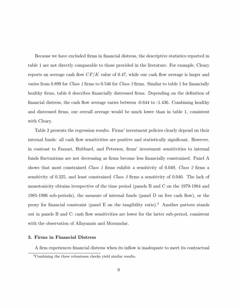
Table 2 presents the regression results. Firms’ investment policies clearly depend on their
internal funds: all cash flow sensitivities are positive and statistically significant. However,
in contrast to Fazzari, Hubbard, and Petersen, firms’ investment sensitivities to internal
funds fluctuations are not decreasing as firms become less financially constrained. Panel A
shows that most constrained Class 1 firms exhibit a sensitivity of 0.049, Class 2 firms a
sensitivity of 0.325, and least constrained Class 3 firms a sensitivity of 0.040. The lack of
monotonicity obtains irrespective of the time period (panels B and C on the 1979-1984 and
1985-1996 sub-periods), the measure of internal funds (panel D on free cash flow), or the
proxy for financial constraint (panel E on the tangibility ratio).4 Another pattern stands
out in panels B and C: cash flow sensitivities are lower for the latter sub-period, consistent
with the observation of Allayannis and Mozumdar.
3. Firms in Financial Distress
A firm experiences financial distress when its inflow is inadequate to meet its contractual
4Combining the three robustness checks yield similar results.
9
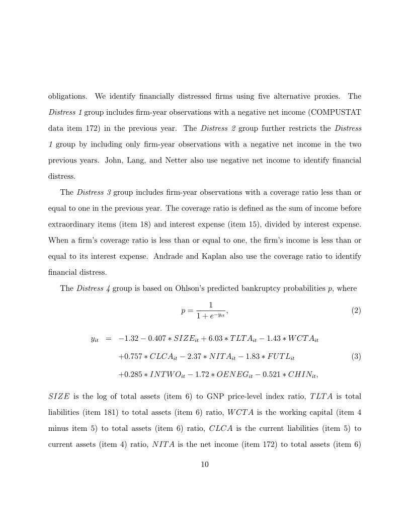
obligations. We identify financially distressed firms using five alternative proxies. The
Distress 1 group includes firm-year observations with a negative net income (COMPUSTAT
data item 172) in the previous year. The Distress 2 group further restricts the Distress
1 group by including only firm-year observations with a negative net income in the two
previous years. John, Lang, and Netter also use negative net income to identify financial
distress.
The Distress 3 group includes firm-year observations with a coverage ratio less than or
equal to one in the previous year. The coverage ratio is defined as the sum of income before
extraordinary items (item 18) and interest expense (item 15), divided by interest expense.
When a firm’s coverage ratio is less than or equal to one, the firm’s income is less than or
equal to its interest expense. Andrade and Kaplan also use the coverage ratio to identify
financial distress.
The Distress 4 group is based on Ohlson’s predicted bankruptcy probabilities p, where
p =1
1 + e−yit, (2)
yit = −1.32− 0.407 ∗ SIZEit + 6.03 ∗ TLTAit − 1.43 ∗WCTAit+0.757 ∗ CLCAit − 2.37 ∗NITAit − 1.83 ∗ FUTLit (3)
+0.285 ∗ INTWOit − 1.72 ∗OENEGit − 0.521 ∗ CHINit,
SIZE is the log of total assets (item 6) to GNP price-level index ratio, TLTA is total
liabilities (item 181) to total assets (item 6) ratio, WCTA is the working capital (item 4
minus item 5) to total assets (item 6) ratio, CLCA is the current liabilities (item 5) to
current assets (item 4) ratio, NITA is the net income (item 172) to total assets (item 6)
10

ratio, FUTL is the funds from operations (item 110) to total liabilities (item 181) ratio,
INTWO is equal to one if net income (item 172) is negative in the previous two years or
zero otherwise, OENEG is equal to one if total liabilities (item 181) are greater than total
assets (item 6) or zero otherwise, CHIN = NIt−NIt−1|NIt|−|NIt−1| , where NIt is the net income (item
172) for year t. The GNP price-level index uses 1968 as a base year, assigning it a value of
100.
The Distress 4 group is obtained from a variant of Ohlson’s bankruptcy probability model.
Because the FUTL variable greatly restricts the sample size, pseudo-bankruptcy probabili-
ties p are calculated by ignoring the effect of FUTL in predicting bankruptcy probabilities:
p =1
1 + e−yit, (4)
where
yit = −1.32− 0.407 ∗ SIZEit + 6.03 ∗ TLTAit − 1.43 ∗WCTAit+0.757 ∗ CLCAit − 2.37 ∗NITAit + 0.285 ∗ INTWOit (5)
−1.72 ∗OENEGit − 0.521 ∗ CHINit.
The Distress 4 group includes firm-year observations with a pseudo-bankruptcy probability
greater than or equal to 50 percent.
The use of Ohlson’s estimated parameters to predict bankruptcy probabilities would be
inappropriate in the presence of structural changes between Ohlson’s study during the 1970-
1976 period and the later 1979-1996 period covered in this paper. To investigate whether
such structural changes may have taken place, we compare the descriptive statistics of our
regressors to those provided by Ohlson. Table 3 confirms that means are indeed quite
11

similar. Panels A and B show that the variable means from Ohlson’s bankrupt firms have
the same magnitude as the variable means from the Distress 4 group. The variable means
from Ohlson’s non-bankrupt firms also have the same magnitude as the variable means
from the remaining COMPUSTAT sample. Structural changes, if any, are not likely to
distort bankruptcy probability predictions. In addition, panel C shows that the bankruptcy
probabilities estimated using all COMPUSTAT manufacturing firms with available data
from 1979 to 1996 are reasonable. About 83 percent of firms have less than a ten percent
bankruptcy probability, while less than six percent of firms have a greater than 50 percent
probability of bankruptcy.
The Distress 5 group is based on Altman’s Z-score. Altman estimates the financial health
of a firm using an overall index Z, where
Z = 0.012X1 + 0.014X2 + 0.033X3 + 0.006X4 + 0.999X5, (6)
X1 is the working capital (item 4 minus item 5) to total assets (item 6) ratio, X2 is the
retained earnings (item 36) to total assets (item 6) ratio, X3 is the earnings before interest
and tax (item 13 minus item 14) to total assets (item 6) ratio, X4 is the market value of
equity (item 24 multiplied by item 25) to total liabilities (item 181) ratio, and X5 is the
sales (item 12) to total assets (item 6) ratio. The Distress 5 group consists of firm-year
observations with Altman’s Z-scores less than one.
As with Ohlson’s estimated bankruptcy probability model, we investigate whether a
structural change may have taken place between Altman’s study covering the 1946-1965
period and the later 1979-1996 period of this paper. Not only does Altman’s data originate
from very long ago, but his sample is also extremely small (33 observations for bankrupt
12
firms and 33 observations for non-bankrupt firms). We compare the descriptive statistics
of our regressors to those provided by Altman. Panels A and B of table 4 shows that the
variable means do differ in magnitude. In addition, panel C shows that Z-scores exhibit
little dispersion: 74 percent of Z-scores are concentrated between the 0.6 and 1.8 values,
and it is rare to observe Z-scores smaller than 0 or larger than 10. Keeping those caveats in
mind, Z-scores are nevertheless explored as a proxy for financial distress.
Table 5 provides a correlation matrix of the different proxies for financial distress. We
expect the net income, coverage ratio, and Z-score to be all positively correlated, and nega-
tively correlated with the pseudo-bankruptcy probability. Indeed, all correlation coefficients
have the expected signs, except for the low but positive correlation between the Z-score and
the pseudo-bankruptcy probability.
Table 6 provides descriptive statistics on financially distressed firms. Similar to the most
financially constrained firms which have a higher Tobin’s Q, a smaller size, and a larger
market-to-book of equity than least constrained firms, distressed firms in turn have a higher
Tobin’s Q, a smaller size, and a larger market-to-book value of equity than most constrained
firms. However, the similarities stop here. In contrast to most financially constrained firms
which invest more, have larger (free) cash flows, a larger income from operations, a lower
leverage, and a higher growth rate of sales than least constrained firms, distressed firms invest
less, have smaller (free) cash flows, a smaller income from operations, a higher leverage, and
a lower growth rate of sales than most constrained firms. It is not surprising to find firms in
financial trouble with lower inflows and a higher leverage than healthy firms. It is also not
surprising to see that firms in distress invest less and grow less rapidly than healthy firms.
13
Financially distressed firms therefore behave differently from financially constrained firms.
Table 6 reports that distressed firms on average experience negative cash flows. For
example, the average cash flow for the Distress 1 firms is -1.071. Healthy firms on average
do not experience negative cash flows. Consistent with our above comparison of distressed
and healthy firms, Allayannis and Mozumdar document that firms with negative cash flows
are smaller, less profitable, have a higher leverage and declining sales.
Table 7 presents the regression results of distressed firms.5 As expected, firms invest more
as investment opportunities improve: Tobin’s Q sensitivities are positive and statistically
significant. In contrast to healthy firms, distressed firms do not rely on their internal funds
to finance their investments: cash flow sensitivities are negative and statistically significant.
Negative cash flow sensitivities imply that financially distressed firms invest more when
their internal funds decrease, and vice versa, that they invest less when their internal funds
increase. Clearly, this behavior does not support the financing hierarchy hypothesis according
to which firms first rely on their internal funds to finance their investment.
Our negative cash flow sensitivity for distressed firms is consistent with the findings
of Allayannis and Mozumdar and Cleary et al. Both papers document a lower cash flow
sensitivity for negative cash flow observations. More specifically, Allayannis and Mozumdar
demonstrate that negative cash flow observations reduce the estimated cash flow sensitivity
of constrained firms, explaining why Cleary obtains a lower cash flow sensitivity for most
constrained firms. When distressed firms are considered with most constrained firms, the
5The free cash flow sensitivity results are similar to the cash flow sensitivity results presented in this
paper. The free cash flow sensitivity results of financially distressed firms are available upon request.
14
negative cash flow sensitivity of distressed firms reduces the cash flow sensitivity of most
constrained firms.
Cleary et al. develop a model of a U-shaped relation between investment and internal
funds. In accord with the model, they empirically document a negative cash flow sensitiv-
ity for the sub-sample of negative cash flow observations and a positive sensitivity for the
sub-sample of positive cash flow observations. We find that the U-shaped relation arises
irrespective of the proxy for financial distress. We consistently obtain a negative cash flow
sensitivity for the sub-sample of distressed firms and a positive sensitivity for healthy firms.
4. Distress from Operations
There appears to exist an overriding phenomenon influencing the investment behavior of
distressed firms — not captured by the traditional financing hierarchy hypothesis. Given that
investment does not respond to internal funds in the expected manner, we examine whether
the investment behavior has more to do with the “real” performance of the firm than with
its financing. More specifically, we investigate whether the investment behavior of distressed
firms is related to their operating performance. When distress is so severe that firms operate
at a loss, their investment policy may be driven by other factors than fluctuations in their
internal funds.
We divide financially distressed firms into two groups: the group of firms with a negative
operating income (item 13) and the group with a positive operating income. Tables 8 and 9
report that firms with operating losses differ substantially from firms with operating profits.
Firms with operating losses invest more, have a higher Tobin’s Q, smaller (free) cash flows,
a smaller size, have a lower leverage, have a higher market-to-book value of equity, and a
15
higher growth rate of sales than firms with operating profits. It is surprising to observe that,
despite their operating losses, these firms invest more (0.356>0.200) and grow at a faster
rate (0.245>0.010).
Panel A of table 10 shows that distressed firms with operating losses have investment
policies that are negatively related to internal funds. The cash flow sensitivity is statistically
significant regardless of the proxy for financial distress. The negative cash flow sensitivity,
inconsistent with the financing hierarchy hypothesis, remains puzzling.
Panel B of table 10 suggests that firms with operating profits have investment policies
that are positively related to internal funds. A positive cash flow sensitivity is consistent
with the financing hierarchy hypothesis as documented in the literature for healthy firms.
For three of the five proxies of financial distress, the cash flow sensitivity is positive and
statistically significant. For Distress 2 firms, the sensitivity is positive but not statistically
significant. For Distress 4 firms, the cash flow sensitivity is not positive. We discount the
conflicting Distress 4 result, as it is obtained from a very small sample size (839 firm-year
observations). We therefore discount this conflicting result.
Another way to define operating profitability is with respect to industry sectors. This
definition assumes that profitable opportunities are systematic to the industry rather than
idiosyncratic to the firm. If an industry suffers from two consecutive years of decreasing
operating income, firms in that industry are classified as bad performers. We expect this
measure to be a very noisy proxy of a firm’s operating performance. Nevertheless, table 11
indicates that the cash flow sensitivity of financially distressed firms is negative and of a
greater magnitude for bad performers than for good ones. Different operating performances
16
again produce different cash flow sensitivities.
Tables 8 and 9 show that firms with operating losses on average experience negative cash
flows. The cash flow average is -1.866 for distressed firms with operating losses versus 0.083
for distressed firms with operating profits. Our cash flow sensitivity results with respect to
operating performance are again consistent with previous findings. In accord with Allayannis
and Mozumdar, the negative cash flow sensitivity of distressed firms with operating losses
reduces the overall positive cash flow sensitivity for financially healthy firms. Restating the
U-shaped investment curve of Cleary et al. in terms of operating performance, we find a
negative cash flow sensitivity for the sub-sample of distressed firms with operating losses and
a positive sensitivity for all other firms.
5. Gamble for Resurrection
We further investigate the negative cash flow sensitivity of distressed firms with oper-
ating losses. Given that such firms are in financial distress and that they do not foresee
any immediate profitable opportunities, they may choose to downsize their operations. In
addition, their investment policy may not react to fluctuations in internal funds, thereby
showing no cash flow sensitivity. We divide the sample of firms in financial distress with
operating losses into two groups: the group of firms that invest less than the previous year
and the group of firms that, against the odds, invest more than the previous year.
Table 12 shows that most firms with operating losses invest less than the previous year.
For the case of Distress 1 firms in panel A, nearly 60 percent of firm-year observations occur
when firms invest less than the previous year. Firms investing less than the previous year
exhibit very little cash flow sensitivity. The cash flow sensitivity is small, but negative
17
and statistically significant for most proxies of financial distress. Firms without immediate
profitable investment opportunities down size operations without much regard to fluctuations
in their internal funds.
However, there remain over 40 percent of firm-year observations characterized by Distress
1 firms with operating losses that nevertheless invest more than the previous year. These
firms display a strong, negative, and statistically significant sensitivity to cash flow. The
negative sensitivity implies that the firms invest more when their cash flows are decreasing.
These results are robust to the different proxies for financial distress. In panels B and
E, Distress 2 and Distress 5 firms that invest less than the previous year have a small but
negative and statistically significant sensitivity. In panels C and D, Distress 3 and Distress
4 firms that invest less than the previous year have in fact a zero cash flow sensitivity,
downsizing irrespective of fluctuations in their internal funds. In all panels, distressed firms
that invest more than the previous year exhibit the strong negative cash flow sensitivity.
The finding that some distressed firms invest more than the previous year when their
cash flows are decreasing is at first surprising. A clue to this puzzle is to emphasize that
an increase in investment takes place when internal funds are decreasing. Necessarily, the
funding for the investment does not originate from internal sources but comes from external
sources. Table 13 reports the main sources and uses of funds for distressed firms. Sources
of funds include the beginning-of-the-period retained earnings RetEarn (item 36), the sale
of property, plant, and equipment SalePPE (item 107), equity issues EIssue (item 108),
and debt issues DIssue (item 111). Uses of funds include cash dividend payments Div
(item 127), investment I (item 128), long-term debt reductions Dred (item 114), and equity
18
repurchases Erep (item 115). All sources and uses are standardized by the firm’s capital
stock K (item 8).
Table 13 shows that the investment is financed by equity claimants. The median firm
with operating losses that invests more than the previous year raises much more funds from
the equity market than the median firm with operating losses that invests less than the
previous year EIssue/K (0.121 > 0.010). Equity claimants invest in their firm despite
difficult financial and operating conditions.
Naturally, the median firm with operating losses that invests more has larger capital
expenditures than the median firm with operating losses that invests less I/K (0.379 >
0.094). Table 13 also shows that it has smaller retained earnings RetEarn/K (−4.572 <−2.200). The retained earnings are negative and of a greater magnitude than the tangibleassets of the firm. This indicates that distressed firms with operating losses have in fact
accumulated losses for some time.
The reliance on equity issues to fund investment is specific to firms with operating losses.
Table 13 shows that, compared to the median firm with operating profits that invests less
than the previous year, the median firm with operating profits that invests more than the
previous year has larger capital expenditures I/K (0.211 > 0.101), smaller retained earnings
RetEarn/K (0.149 < 0.250), but about the same minimal amount of equity issuesEIssue/K
(0.003 ≈ 0.000).In fact, among the distressed firms that invest more than the previous year, the ones
with operating losses differ from those with operating profits in terms of their investment,
retained earnings, and equity issues. The median firm with operating losses has smaller
19
retained earnings (−4.572 < 0.149), invests more (0.379 > 0.211), and relies more on equityissues to fund the investment (0.121 > 0.003). In other words, firms with operating losses
invest more and have less internal funds to finance their investment. Instead, they turn to
equity claimants.
The evidence is consistent with Jensen and Meckling’s asset substitution problem. Be-
cause equity claimants are protected by limited liability, they prefer riskier projects to those
maximizing total firm value. In our context, they finance the increased investment of finan-
cially distressed firms operating at a loss.
Decamps and Faure-Grimaud (2000) describe the gamble for resurrection as an agency
problem arising when equity claimants of a distressed firm decide to continue operations
when liquidation would have been optimal. Continuing operations allows equity claimants
to be exposed to future uncertain but perhaps better operating conditions. Equity claimants
hope that some fortunate event occurs and lifts the value of their claims. In such distress,
equity claimants who are protected by limited liability may have very little to lose, and thus
gamble for resurrection.
Our evidence complements the work of Andrade and Kaplan. In their sample of distressed
firms with operating profits, they do not find support for any risk shifting behavior. Indeed,
we uncover evidence consistent with the agency problem only for a subset of distressed firms
with operating losses.
6. Conclusion
The relation between investment and internal funds for financially distressed firms is
diverse. First, they exhibit a positive cash flow sensitivity if firms operate at a profit, similar
20
to the cash flow sensitivity results already documented in the literature for financially healthy
firms. Second, they exhibit little cash flow sensitivity if firms operate at a loss and invest
less than the previous year. Third, they exhibit a strong negative cash flow sensitivity if
firms operate at a loss but nevertheless invest more than the previous year.
Our results clearly emphasize that not all manufacturing firms rely on their internal funds
to finance their investments. The increase in investment of financially distressed firms with
operating losses is funded by equity claimants. Equity claimants may lose from providing
financing to an unprofitable firm, but nevertheless gamble for the firm’s resurrection. Equity
claimants bet that this investment allows for the possibility of a good event turning around
the fortunes of the firm. Thus, for this group of firms, the gamble for resurrection appears to
overrule the financing hierarchy hypothesis as an explanation of firms’ investment behavior.
Further empirical research into the gamble for resurrection would be helpful.
Acknowledgements
We would like to thank seminar participants at the University of Colorado at Boulder
for helpful comments.
References
Allayannis, G., and A. Mozumdar, 2004, The impact of negative cash flow and influential
observations on investment-cash flow sensitivity estimates, Journal of Banking and Finance
28, 901-930.
Altman, E.I., 1968, Financial ratios, discriminant analysis and the prediction of corporate
bankruptcy, Journal of Finance 23, 589-609.
21

Andrade, G., and S.N. Kaplan, 1998, How costly is financial (not economic) distress? Ev-
idence from highly leveraged transactions that became distressed, Journal of Finance 53,
1443-1493.
Cleary, S., 1999, The relationship between firm investment and financial status, Journal of
Finance 54, 673-692.
Cleary, S., P. Povel, and M. Raith, 2004, The U-shaped investment curve: Theory and evi-
dence, Working Paper from St. Mary’s University, University of Minnesota, and University
of Rochester.
Decamps, J.-P., and A. Faure-Grimaud, 2000, Bankruptcy costs, ex post renegotiation and
gambling for resurrection, Finance 21, 71-84.
Fazzari, S.M., R.G. Hubbard, and B.C. Petersen, 2000, Investment-cash flow sensitivities are
useful: A comment on Kaplan and Zingales, Quarterly Journal of Economics 115, 695-705.
Fazzari, S.M., R.G. Hubbard, and B.C. Petersen, 1988, Financing constraints and corporate
investment, Brookings Paper on Economic Activity 1, 141-195.
Gilchrist, S., and C.P. Himmelberg, 1995, Evidence on the role of cash flow in reduced-form
investment equations, Journal of Monetary Economics 36, 541-572.
Gul, F.A., and J.S.L. Tsui, 1998, A test of the free cash flow and debt monitoring hypotheses:
Evidence from audit pricing, Journal of Accounting and Economics 24, 219-237.
Hoshi, T., A.K. Kashyap, and D. Scharfstein, 1991, Corporate structure, liquidity, and
investment: Evidence from Japanese panel data, Quarterly Journal of Economics 106, 33-
60.
22
Hubbard, R.G., 1998, Capital-market imperfections and investment, Journal of Economic
Literature 36, 193-225.
Jensen, M.C., and W.H. Meckling, 1976, Theory of the firm: Managerial behavior, agency
costs and ownership structure, Journal of Financial Economics 3, 305-360.
John, K., L.H.P. Lang, and J. Netter, 1992, The voluntary restructuring of large firms in
response to performance decline, Journal of Finance 47, 891-918.
Kadapakkam, P.-R., P.C. Kumar, and L.A. Riddick, 1998, The impact of cash flows and
firm size on investment: The international evidence, Journal of Banking and Finance 22,
293-320.
Kaplan, S.N., and L. Zingales, 2000, Investment-cash flow sensitivities are not valid measures
of financing constraints, Quarterly Journal of Economics 115, 707-712.
Kaplan, S.N., and L. Zingales, 1997, Do Investment-cash flow sensitivities provide useful
measures of financing constraints? Quarterly Journal of Economics 112, 169-215.
Moyen, N., 2004, Investment-cash flow sensitivities: Constrained versus unconstrained firms,
Journal of Finance 59, 2061-2092.
Myers, S.C., and N.S. Majluf, 1984, Corporate financing and investment decisions when firms
have information that investors do not have, Journal of Financial Economics 13, 187-221.
Ohlson, J.A., 1980, Financial ratios and the probabilistic prediction of bankruptcy, Journal
of Accounting Research 18, 109-131.
Oliner, S.D., and G.D. Rudebusch, 1992, Sources of the financing hierarchy for business
investment, Review of Economics and Statistics 74, 643-654.
23

Schaller, H., 1993, Asymmetric information, liquidity constraints, and Canadian investment,
Canadian Journal of Economics 26, 552-574.
24
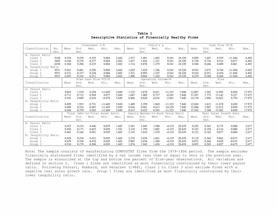
Table 1 Descriptive Statistics of Financially Healthy Firms
Investment I/K Tobin’s Q Cash Flow CF/K
Classification No. obs.
Mean Std. Dev.
Med. Min. Max. Mean Std. Dev.
Med. Min. Max. Mean Std. Dev.
Med. Min. Max.
A. Payout Ratio Class 1 9168 0.534 0.539 0.355 0.004 2.682 1.975 1.491 1.482 0.541 10.320 0.899 1.607 0.559 -11.844 6.492Class 2 2045 0.346 0.276 0.277 0.004 2.682 1.627 1.026 1.331 0.541 10.320 0.720 0.736 0.516 0.077 6.492Class 3 6350 0.268 0.206 0.225 0.004 2.682 1.514 0.858 1.279 0.541 10.320 0.546 0.646 0.409 0.061 6.492
B. Tangibility Ratio Group 1 9551 0.453 0.481 0.296 0.004 2.682 1.829 1.429 1.346 0.541 10.320 0.932 2.072 0.744 -11.844 6.492Group 2 9551 0.321 0.337 0.228 0.004 2.682 1.521 0.995 1.225 0.541 10.320 0.410 0.551 0.410 -11.844 6.492Group 3 9551 0.291 0.316 0.211 0.004 2.682 1.408 0.884 1.162 0.541 10.320 0.270 0.388 0.264 -11.844 6.492
Free Cash Flow FCF/K Operating Income/K Size Classification Mean Std.
Dev. Med. Min. Max. Mean Std.
Dev. Med. Min. Max. Mean Std.
Dev. Med. Min. Max.
A. Payout Ratio Class 1 0.865 1.510 0.544 -11.669 5.849 1.325 1.870 0.811 -11.323 7.840 12.007 1.582 11.895 8.050 17.975Class 2 0.711 0.712 0.509 0.077 5.849 1.047 1.009 0.757 -0.201 7.840 13.287 1.775 13.142 9.237 17.975Class 3 0.541 0.609 0.410 -0.478 5.849 0.804 0.828 0.616 -2.441 7.840 14.118 1.886 14.022 8.570 17.975
B. Tangibility Ratio Group 1 0.899 1.953 0.731 -11.669 5.849 1.409 2.299 1.069 -11.323 7.840 12.030 1.812 11.878 8.050 17.975Group 2 0.409 0.524 0.407 -11.669 5.849 0.656 0.601 0.613 -10.220 7.840 12.986 1.907 12.815 8.050 17.975Group 3 0.268 0.370 0.262 -11.669 5.849 0.413 0.423 0.383 -11.323 7.840 13.562 2.100 13.462 8.050 17.975
Total Debt-to-Total Asset Ratio Equity Market-to-Book Value Ratio Real Sales Growth Rate Classification Mean Std.
Dev. Med. Min. Max. Mean Std.
Dev. Med. Min. Max. Mean Std.
Dev. Med. Min. Max.
A. Payout Ratio Class 1 0.452 0.214 0.446 0.059 1.685 2.561 2.445 1.940 -4.319 20.439 0.283 0.365 0.175 0.000 2.677Class 2 0.456 0.171 0.455 0.059 1.541 2.210 1.799 1.802 -4.319 20.439 0.167 0.194 0.116 0.000 2.677Class 3 0.481 0.166 0.491 0.059 1.685 2.145 1.810 1.670 -4.319 20.439 0.123 0.182 0.077 0.000 2.677
B. Tangibility Ratio Group 1 0.428 0.234 0.412 0.059 1.685 2.276 2.434 1.601 -4.319 20.439 0.119 0.366 0.062 -0.675 2.677Group 2 0.478 0.194 0.476 0.059 1.685 2.003 2.034 1.508 -4.319 20.439 0.072 0.266 0.038 -0.675 2.677Group 3 0.510 0.179 0.508 0.059 1.685 1.874 1.942 1.424 -4.319 20.439 0.053 0.245 0.027 -0.675 2.677
Note: The sample consists of manufacturing COMPUSTAT firms from the 1979-1996 period. The sample excludes financially distressed firms identified by a net income less than or equal to zero in the previous year. The sample is winsorized at the top and bottom one percent of firm-year observations. All variables are defined in section 2. Class 1 firms are identified as most financially constrained by their lower payout ratio. Following Fazzari, Hubbard, and Petersen (1988), Class 1 to Class 3 also exclude firms with a negative real sales growth rate. Group 1 firms are identified as most financially constrained by their lower tangibility ratio.
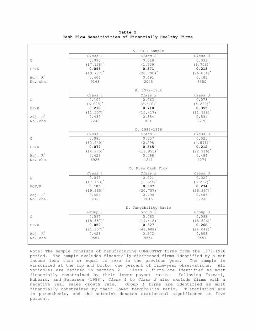
Table 2 Cash Flow Sensitivities of Financially Healthy Firms
A. Full Sample Class 1 Class 2 Class 3 Q 0.098
(17.138)* 0.018 (1.739)
0.031 (6.706)*
CF/K 0.096 (19.787)*
0.371 (20.798)*
0.213 (26.034)*
Adj. R2 0.406 0.491 0.481 No. obs. 9168 2045 6350 B. 1979-1984 Class 1 Class 2 Class 3 Q 0.109
(6.608)* 0.063
(2.416)* 0.078
(5.229)* CF/K 0.218
(11.507)* 0.718
(15.417)* 0.355
(11.928)* Adj. R2 0.439 0.554 0.531 No. obs. 2242 804 2276 C. 1985-1996
Class 1 Class 2 Class 3 Q 0.085
(12.440)* 0.007 (0.598)
0.025 (4.571)*
CF/K 0.079 (14.975)*
0.345 (11.955)*
0.212 (22.916)*
Adj. R2 0.429 0.568 0.484 No. obs. 6926 1241 4074 D. Free Cash Flow Class 1 Class 2 Class 3 Q 0.098
(17.153)* 0.021
(2.027)* 0.029
(6.232)* FCF/K 0.105
(19.965)* 0.387
(20.757)* 0.234
(26.397)* Adj. R2 0.406 0.490 0.483 No. obs. 9166 2045 6350 E. Tangibility Ratio
Group 1 Group 2 Group 3 Q 0.097
(18.557)* 0.063
(14.418)* 0.093
(18.526)* CF/K 0.059
(21.357)* 0.327
(46.688)* 0.268
(24.042)* Adj. R2 0.428 0.572 0.503 No. obs. 9551 9551 9551 Note: The sample consists of manufacturing COMPUSTAT firms from the 1979-1996 period. The sample excludes financially distressed firms identified by a net income less than or equal to zero in the previous year. The sample is winsorized at the top and bottom one percent of firm-year observations. All variables are defined in section 2. Class 1 firms are identified as most financially constrained by their lower payout ratio. Following Fazzari, Hubbard, and Petersen (1988), Class 1 to Class 3 also exclude firms with a negative real sales growth rate. Group 1 firms are identified as most financially constrained by their lower tangibility ratio. T-statistics are in parenthesis, and the asterisk denotes statistical significance at five percent.

Table 3
Ohlson’s (1980) Bankruptcy Probabilities
A. Descriptive Statistics from Ohlson’s Sample
Bankrupt Firms Non-bankrupt Firms Mean Std. Dev. Mean Std. Dev. Size 12.134 1.380 13.260 1.570 TLTA 0.905 0.637 0.488 0.181 WCTA 0.041 0.608 0.310 0.182 CLCA 1.320 2.520 0.525 0.740 NITA -0.208 0.411 0.053 0.076 FUTL -0.117 0.421 0.281 0.360 INTWO 0.390 0.488 0.043 0.203 OENEG 0.180 0.385 0.004 0.066 CHIN -0.322 0.644 0.038 0.458 B. Descriptive Statistics from our Sample
Distress 4 Firms Healthy Firms Mean Std. Dev. Mean Std. Dev.
Size 10.971 1.746 12.980 2.022 TLTA 0.765 0.565 0.431 0.156 WCTA 0.159 0.506 0.377 0.177 CLCA 0.980 4.075 0.417 0.207 NITA -0.205 0.524 0.068 0.116 FUTL -0.295 1.055 0.340 0.460 INTWO 0.442 0.497 0.034 0.180 OENEG 0.108 0.310 0.001 0.028 CHIN -0.266 0.633 0.080 0.456
C. Distribution of Bankruptcy Probabilities
Bankruptcy Cumulative Cumulative Probability Frequency Percent Frequency Percent 0.0 ≤ p < 0.1 15305 83.19 15305 83.19 0.1 ≤ p < 0.2 900 4.89 16205 88.08 0.2 ≤ p < 0.3 445 2.42 16650 90.50 0.3 ≤ p < 0.4 292 1.59 16942 92.09 0.4 ≤ p < 0.5 231 1.26 17173 93.34 0.5 ≤ p < 0.6 161 0.88 17334 94.22 0.6 ≤ p < 0.7 154 0.84 17488 95.05 0.7 ≤ p < 0.8 176 0.96 17664 96.01 0.8 ≤ p < 0.9 178 0.97 17842 96.98 0.9 ≤ p ≤ 1.0 556 3.02 18398 100.00
Note: The sample consists of manufacturing COMPUSTAT firms from the 1979-1996 period. Distress 4 firms are identified by pseudo-bankruptcy probabilities greater or equal to 50 percent. All variables are defined in section 3.
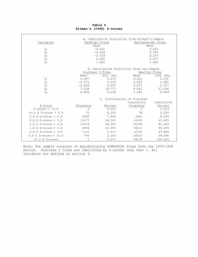
Table 4 Altman’s (1968) Z-scores
A. Descriptive Statistics from Altman’s Sample
Variables Bankrupt Firms Non-bankrupt Firms Mean Mean
X1 -0.061 0.414 X2 -0.626 0.355 X3 -0.318 0.153 X4 0.401 2.477 X5 1.500 1.900
B. Descriptive Statistics from our Sample
Distress 5 Firms Healthy Firms Mean Std. Dev. Mean Std. Dev. X1 0.297 0.372 0.322 0.331 X2 -0.571 3.163 0.029 1.681 X3 -0.099 0.407 0.072 0.217 X4 7.538 14.777 4.662 27.044 X5 0.626 0.258 1.565 0.649
C. Distribution of Z-scores Cumulative Cumulative
Z-score Frequency Percent Frequency Percent Z-score < -0.6 3 0.01% 3 0.01%
-0.6 ≤ Z-score < 0.0 75 0.20% 78 0.20% 0.0 ≤ Z-score < 0.6 2985 7.83% 3063 8.03% 0.6 ≤ Z-score < 1.2 13177 34.56% 16240 42.60% 1.2 ≤ Z-score < 1.8 15018 39.39% 31258 81.99% 1.8 ≤ Z-score < 2.4 4954 12.99% 36212 94.98% 2.4 ≤ Z-score < 3.0 1110 2.91% 37322 97.89% 3.0 ≤ Z-score < 10.0 799 2.10% 38121 99.99%
10.0 ≤ Z-score 5 0.01% 38126 100.00%
Note: The sample consists of manufacturing COMPUSTAT firms from the 1979-1996 period. Distress 5 firms are identified by Z-scores less than 1. All variables are defined in section 3.
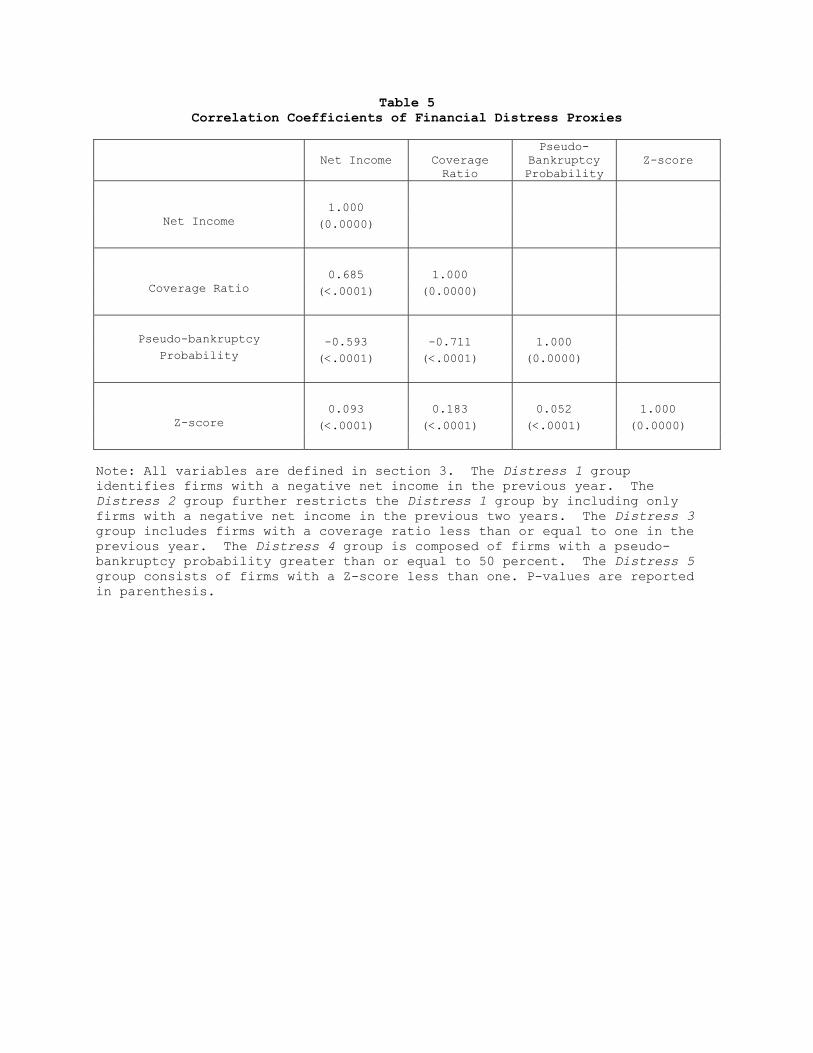
Table 5 Correlation Coefficients of Financial Distress Proxies
Net Income
Coverage Ratio
Pseudo-Bankruptcy Probability
Z-score
1.000
Net Income (0.0000) 0.685 1.000
Coverage Ratio (<.0001) (0.0000)
Pseudo-bankruptcy -0.593 -0.711 1.000 Probability (<.0001) (<.0001) (0.0000)
0.093 0.183 0.052 1.000
Z-score (<.0001) (<.0001) (<.0001) (0.0000)
Note: All variables are defined in section 3. The Distress 1 group identifies firms with a negative net income in the previous year. The Distress 2 group further restricts the Distress 1 group by including only firms with a negative net income in the previous two years. The Distress 3 group includes firms with a coverage ratio less than or equal to one in the previous year. The Distress 4 group is composed of firms with a pseudo-bankruptcy probability greater than or equal to 50 percent. The Distress 5 group consists of firms with a Z-score less than one. P-values are reported in parenthesis.
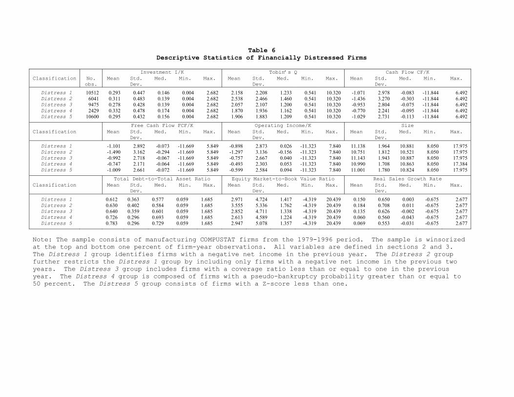
Table 6 Descriptive Statistics of Financially Distressed Firms
Investment I/K Tobin’s Q Cash Flow CF/K
Classification No. obs.
Mean Std. Dev.
Med. Min. Max. Mean Std. Dev.
Med. Min. Max. Mean Std. Dev.
Med. Min. Max.
Distress 1 10512 0.293 0.447 0.146 0.004 2.682 2.158 2.208 1.233 0.541 10.320 -1.071 2.978 -0.083 -11.844 6.492 Distress 2 6041 0.311 0.483 0.139 0.004 2.682 2.538 2.466 1.460 0.541 10.320 -1.436 3.270 -0.303 -11.844 6.492 Distress 3 9475 0.278 0.428 0.139 0.004 2.682 2.057 2.107 1.200 0.541 10.320 -0.953 2.804 -0.075 -11.844 6.492 Distress 4 2429 0.332 0.478 0.174 0.004 2.682 1.870 1.936 1.162 0.541 10.320 -0.770 2.241 -0.095 -11.844 6.492 Distress 5 10600 0.295 0.432 0.156 0.004 2.682 1.906 1.883 1.209 0.541 10.320 -1.029 2.731 -0.113 -11.844 6.492
Free Cash Flow FCF/K Operating Income/K Size Classification Mean Std.
Dev. Med. Min. Max. Mean Std.
Dev. Med. Min. Max. Mean Std.
Dev. Med. Min. Max.
Distress 1 -1.101 2.892 -0.073 -11.669 5.849 -0.898 2.873 0.026 -11.323 7.840 11.138 1.964 10.881 8.050 17.975 Distress 2 -1.490 3.162 -0.294 -11.669 5.849 -1.297 3.136 -0.156 -11.323 7.840 10.751 1.812 10.521 8.050 17.975 Distress 3 -0.992 2.718 -0.067 -11.669 5.849 -0.757 2.667 0.040 -11.323 7.840 11.143 1.943 10.887 8.050 17.975 Distress 4 -0.747 2.171 -0.064 -11.669 5.849 -0.493 2.303 0.053 -11.323 7.840 10.990 1.708 10.863 8.050 17.384 Distress 5 -1.009 2.661 -0.072 -11.669 5.849 -0.599 2.584 0.094 -11.323 7.840 11.001 1.780 10.824 8.050 17.975
Total Debt-to-Total Asset Ratio Equity Market-to-Book Value Ratio Real Sales Growth Rate Classification Mean Std.
Dev. Med. Min. Max. Mean Std.
Dev. Med. Min. Max. Mean Std.
Dev. Med. Min. Max.
Distress 1 0.612 0.363 0.577 0.059 1.685 2.971 4.724 1.417 -4.319 20.439 0.150 0.650 0.003 -0.675 2.677 Distress 2 0.630 0.402 0.584 0.059 1.685 3.555 5.336 1.762 -4.319 20.439 0.184 0.708 0.011 -0.675 2.677 Distress 3 0.640 0.359 0.601 0.059 1.685 2.852 4.711 1.338 -4.319 20.439 0.135 0.626 -0.002 -0.675 2.677 Distress 4 0.726 0.296 0.693 0.059 1.685 2.613 4.589 1.224 -4.319 20.439 0.060 0.560 -0.043 -0.675 2.677 Distress 5 0.783 0.296 0.729 0.059 1.685 2.947 5.078 1.357 -4.319 20.439 0.069 0.553 -0.031 -0.675 2.677
Note: The sample consists of manufacturing COMPUSTAT firms from the 1979-1996 period. The sample is winsorized at the top and bottom one percent of firm-year observations. All variables are defined in sections 2 and 3. The Distress 1 group identifies firms with a negative net income in the previous year. The Distress 2 group further restricts the Distress 1 group by including only firms with a negative net income in the previous two years. The Distress 3 group includes firms with a coverage ratio less than or equal to one in the previous year. The Distress 4 group is composed of firms with a pseudo-bankruptcy probability greater than or equal to 50 percent. The Distress 5 group consists of firms with a Z-score less than one.
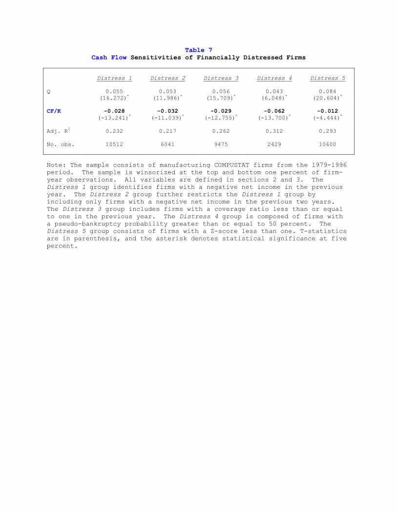
Table 7 Cash Flow Sensitivities of Financially Distressed Firms
Distress 1 Distress 2 Distress 3 Distress 4 Distress 5
Q 0.055 (16.272)*
0.053 (11.986)*
0.056 (15.709)*
0.043 (6.048)*
0.084 (20.604)*
CF/K -0.028
(-13.241)* -0.032
(-11.039)* -0.029
(-12.755)* -0.062
(-13.700)* -0.012
(-4.444)* Adj. R2 0.232
0.217 0.262 0.312 0.293
No. obs. 10512 6041 9475 2429 10600
Note: The sample consists of manufacturing COMPUSTAT firms from the 1979-1996 period. The sample is winsorized at the top and bottom one percent of firm-year observations. All variables are defined in sections 2 and 3. The Distress 1 group identifies firms with a negative net income in the previous year. The Distress 2 group further restricts the Distress 1 group by including only firms with a negative net income in the previous two years. The Distress 3 group includes firms with a coverage ratio less than or equal to one in the previous year. The Distress 4 group is composed of firms with a pseudo-bankruptcy probability greater than or equal to 50 percent. The Distress 5 group consists of firms with a Z-score less than one. T-statistics are in parenthesis, and the asterisk denotes statistical significance at five percent.
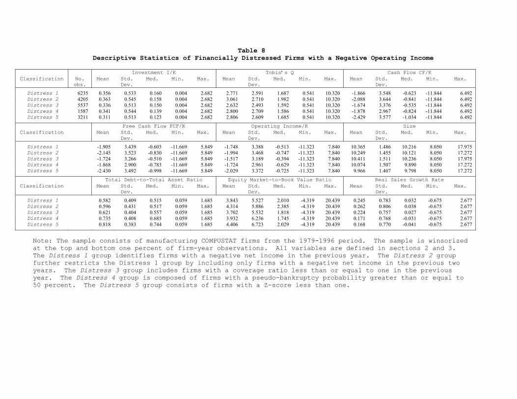
Table 8 Descriptive Statistics of Financially Distressed Firms with a Negative Operating Income
Investment I/K Tobin’s Q Cash Flow CF/K
Classification No. obs.
Mean Std. Dev.
Med. Min. Max. Mean Std. Dev.
Med. Min. Max. Mean Std. Dev.
Med. Min. Max.
Distress 1 6235 0.356 0.533 0.160 0.004 2.682 2.771 2.591 1.687 0.541 10.320 -1.866 3.548 -0.623 -11.844 6.492 Distress 2 4205 0.363 0.545 0.158 0.004 2.682 3.061 2.710 1.982 0.541 10.320 -2.088 3.644 -0.841 -11.844 6.492 Distress 3 5537 0.336 0.513 0.150 0.004 2.682 2.632 2.493 1.592 0.541 10.320 -1.674 3.376 -0.535 -11.844 6.492 Distress 4 1587 0.341 0.544 0.139 0.004 2.682 2.800 2.709 1.586 0.541 10.320 -1.878 2.967 -0.824 -11.844 6.492 Distress 5 3211 0.311 0.513 0.123 0.004 2.682 2.806 2.609 1.685 0.541 10.320 -2.429 3.577 -1.034 -11.844 6.492
Free Cash Flow FCF/K Operating Income/K Size Classification Mean Std.
Dev. Med. Min. Max. Mean Std.
Dev. Med. Min. Max. Mean Std.
Dev. Med. Min. Max.
Distress 1 -1.905 3.439 -0.603 -11.669 5.849 -1.748 3.388 -0.513 -11.323 7.840 10.365 1.486 10.216 8.050 17.975 Distress 2 -2.145 3.523 -0.830 -11.669 5.849 -1.994 3.468 -0.747 -11.323 7.840 10.249 1.455 10.121 8.050 17.272 Distress 3 -1.724 3.266 -0.510 -11.669 5.849 -1.517 3.189 -0.394 -11.323 7.840 10.411 1.511 10.236 8.050 17.975 Distress 4 -1.868 2.900 -0.783 -11.669 5.849 -1.724 2.961 -0.629 -11.323 7.840 10.074 1.507 9.890 8.050 17.272 Distress 5 -2.430 3.492 -0.998 -11.669 5.849 -2.029 3.372 -0.725 -11.323 7.840 9.966 1.407 9.798 8.050 17.272
Total Debt-to-Total Asset Ratio Equity Market-to-Book Value Ratio Real Sales Growth Rate Classification Mean Std.
Dev. Med. Min. Max. Mean Std.
Dev. Med. Min. Max. Mean Std.
Dev. Med. Min. Max.
Distress 1 0.582 0.409 0.515 0.059 1.685 3.843 5.527 2.010 -4.319 20.439 0.245 0.783 0.032 -0.675 2.677 Distress 2 0.596 0.431 0.517 0.059 1.685 4.314 5.886 2.385 -4.319 20.439 0.262 0.806 0.038 -0.675 2.677 Distress 3 0.621 0.404 0.557 0.059 1.685 3.702 5.532 1.818 -4.319 20.439 0.224 0.757 0.027 -0.675 2.677 Distress 4 0.735 0.408 0.685 0.059 1.685 3.932 6.236 1.745 -4.319 20.439 0.171 0.768 -0.031 -0.675 2.677 Distress 5 0.818 0.383 0.744 0.059 1.685 4.406 6.723 2.029 -4.319 20.439 0.168 0.770 -0.041 -0.675 2.677
Note: The sample consists of manufacturing COMPUSTAT firms from the 1979-1996 period. The sample is winsorized at the top and bottom one percent of firm-year observations. All variables are defined in sections 2 and 3. The Distress 1 group identifies firms with a negative net income in the previous year. The Distress 2 group further restricts the Distress 1 group by including only firms with a negative net income in the previous two years. The Distress 3 group includes firms with a coverage ratio less than or equal to one in the previous year. The Distress 4 group is composed of firms with a pseudo-bankruptcy probability greater than or equal to 50 percent. The Distress 5 group consists of firms with a Z-score less than one.

Table 9 Descriptive Statistics of Financially Distressed Firms with a Positive Operating Income
Investment I/K Tobin’s Q Cash Flow CF/K
Classification No. obs.
Mean Std. Dev.
Med. Min. Max. Mean Std. Dev.
Med. Min. Max. Mean Std. Dev.
Med. Min. Max.
Distress 1 4255 0.200 0.248 0.135 0.004 2.682 1.261 0.908 1.034 0.541 10.320 0.083 1.067 0.149 -11.844 6.492 Distress 2 1822 0.189 0.254 0.117 0.004 2.682 1.336 1.045 1.061 0.541 10.320 0.042 1.221 0.124 -11.844 6.492 Distress 3 3918 0.189 0.254 0.117 0.004 2.682 1.336 1.045 1.061 0.541 10.320 0.042 1.221 0.124 -11.844 6.492 Distress 4 839 0.326 0.435 0.186 0.004 2.682 1.347 0.992 1.063 0.541 10.320 -0.147 1.350 0.055 -11.844 6.492 Distress 5 7376 0.284 0.376 0.170 0.004 2.682 1.388 0.971 1.108 0.541 10.320 -0.226 1.620 0.069 -11.844 6.492
Free Cash Flow FCF/K Operating Income/K Size Classification Mean Std.
Dev. Med. Min. Max. Mean Std.
Dev. Med. Min. Max. Mean Std.
Dev. Med. Min. Max.
Distress 1 0.077 0.961 0.151 -11.669 5.849 0.343 0.962 0.275 -11.323 7.840 12.278 2.026 12.026 8.050 17.975 Distress 2 0.020 1.044 0.121 -11.669 5.849 0.306 1.022 0.250 -11.323 7.840 11.919 2.011 11.627 8.050 17.975 Distress 3 0.020 1.044 0.121 -11.669 5.849 0.306 1.022 0.250 -11.323 7.840 11.919 2.011 11.627 8.050 17.975 Distress 4 -0.116 1.235 0.071 -11.669 5.849 0.197 1.424 0.210 -11.323 7.840 11.505 1.595 11.352 8.050 17.384 Distress 5 -0.190 1.515 0.090 -11.669 5.849 0.221 1.460 0.265 -11.323 7.840 11.598 1.697 11.445 8.050 17.975
Total Debt-to-Total Asset Ratio Equity Market-to-Book Value Ratio Real Sales Growth Rate Classification Mean Std.
Dev. Med. Min. Max. Mean Std.
Dev. Med. Min. Max. Mean Std.
Dev. Med. Min. Max.
Distress 1 0.656 0.277 0.631 0.059 1.685 1.723 2.818 1.094 -4.319 20.439 0.010 0.330 -0.018 -0.675 2.677 Distress 2 0.709 0.314 0.674 0.059 1.685 1.847 3.239 1.098 -4.319 20.439 0.002 0.333 -0.021 -0.675 2.677 Distress 3 0.709 0.314 0.674 0.059 1.685 1.847 3.239 1.098 -4.319 20.439 0.002 0.333 -0.021 -0.675 2.677 Distress 4 0.722 0.209 0.695 0.059 1.685 1.900 3.162 1.098 -4.319 20.439 -0.003 0.381 -0.046 -0.675 2.677 Distress 5 0.763 0.229 0.725 0.126 1.685 2.140 3.639 1.222 -4.319 20.439 0.011 0.362 -0.029 -0.675 2.677
Note: The sample consists of manufacturing COMPUSTAT firms from the 1979-1996 period. The sample is winsorized at the top and bottom one percent of firm-year observations. All variables are defined in sections 2 and 3. The Distress 1 group identifies firms with a negative net income in the previous year. The Distress 2 group further restricts the Distress 1 group by including only firms with a negative net income in the previous two years. The Distress 3 group includes firms with a coverage ratio less than or equal to one in the previous year. The Distress 4 group is composed of firms with a pseudo-bankruptcy probability greater than or equal to 50 percent. The Distress 5 group consists of firms with a Z-score less than one.
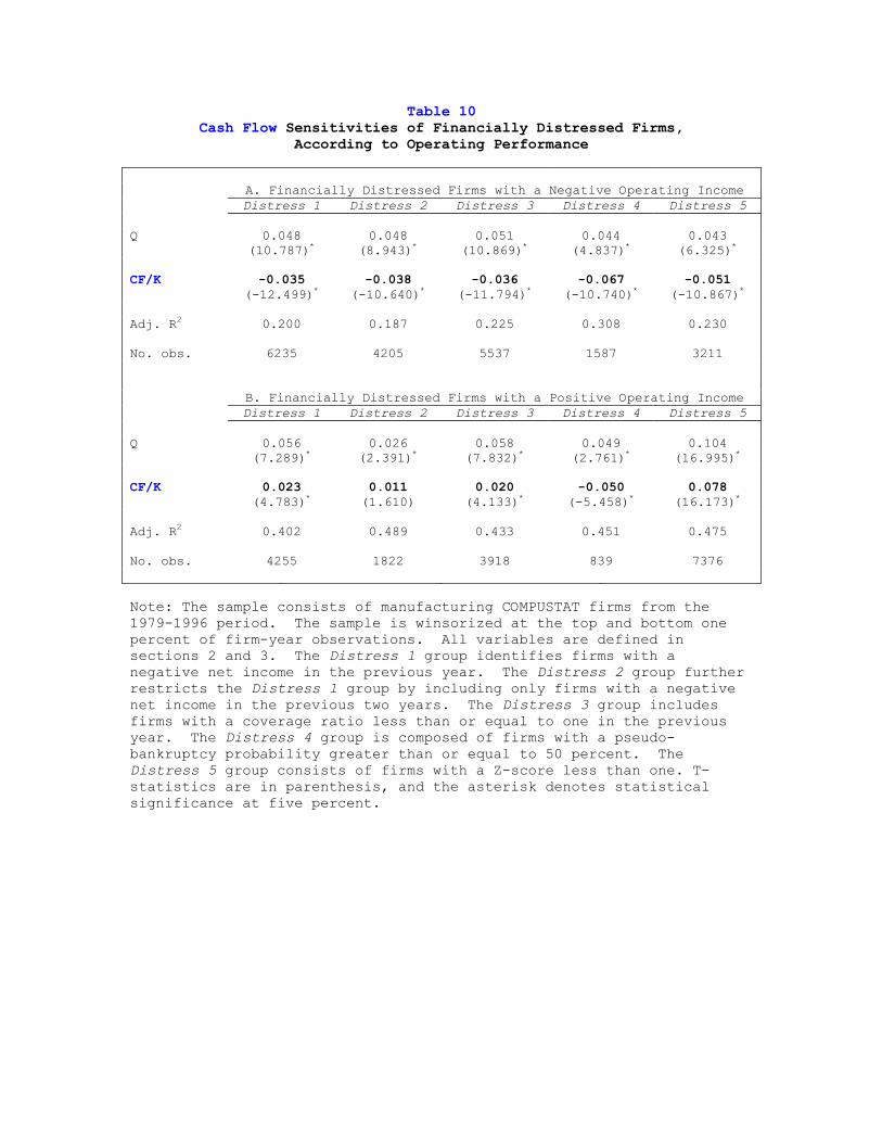
Table 10 Cash Flow Sensitivities of Financially Distressed Firms,
According to Operating Performance
A. Financially Distressed Firms with a Negative Operating Income Distress 1 Distress 2 Distress 3 Distress 4 Distress 5
Q 0.048
(10.787)* 0.048
(8.943)* 0.051
(10.869)* 0.044
(4.837)* 0.043
(6.325)* CF/K -0.035
(-12.499)* -0.038
(-10.640)* -0.036
(-11.794)* -0.067
(-10.740)* -0.051
(-10.867)* Adj. R2 0.200
0.187 0.225
0.308 0.230
No. obs. 6235 4205 5537 1587 3211 B. Financially Distressed Firms with a Positive Operating Income Distress 1 Distress 2 Distress 3 Distress 4 Distress 5
Q 0.056
(7.289)* 0.026
(2.391)* 0.058
(7.832)* 0.049
(2.761)* 0.104
(16.995)* CF/K 0.023
(4.783)* 0.011 (1.610)
0.020 (4.133)*
-0.050 (-5.458)*
0.078 (16.173)*
Adj. R2 0.402
0.489 0.433 0.451 0.475
No. obs. 4255 1822 3918 839 7376 Note: The sample consists of manufacturing COMPUSTAT firms from the 1979-1996 period. The sample is winsorized at the top and bottom one percent of firm-year observations. All variables are defined in sections 2 and 3. The Distress 1 group identifies firms with a negative net income in the previous year. The Distress 2 group further restricts the Distress 1 group by including only firms with a negative net income in the previous two years. The Distress 3 group includes firms with a coverage ratio less than or equal to one in the previous year. The Distress 4 group is composed of firms with a pseudo-bankruptcy probability greater than or equal to 50 percent. The Distress 5 group consists of firms with a Z-score less than one. T-statistics are in parenthesis, and the asterisk denotes statistical significance at five percent.
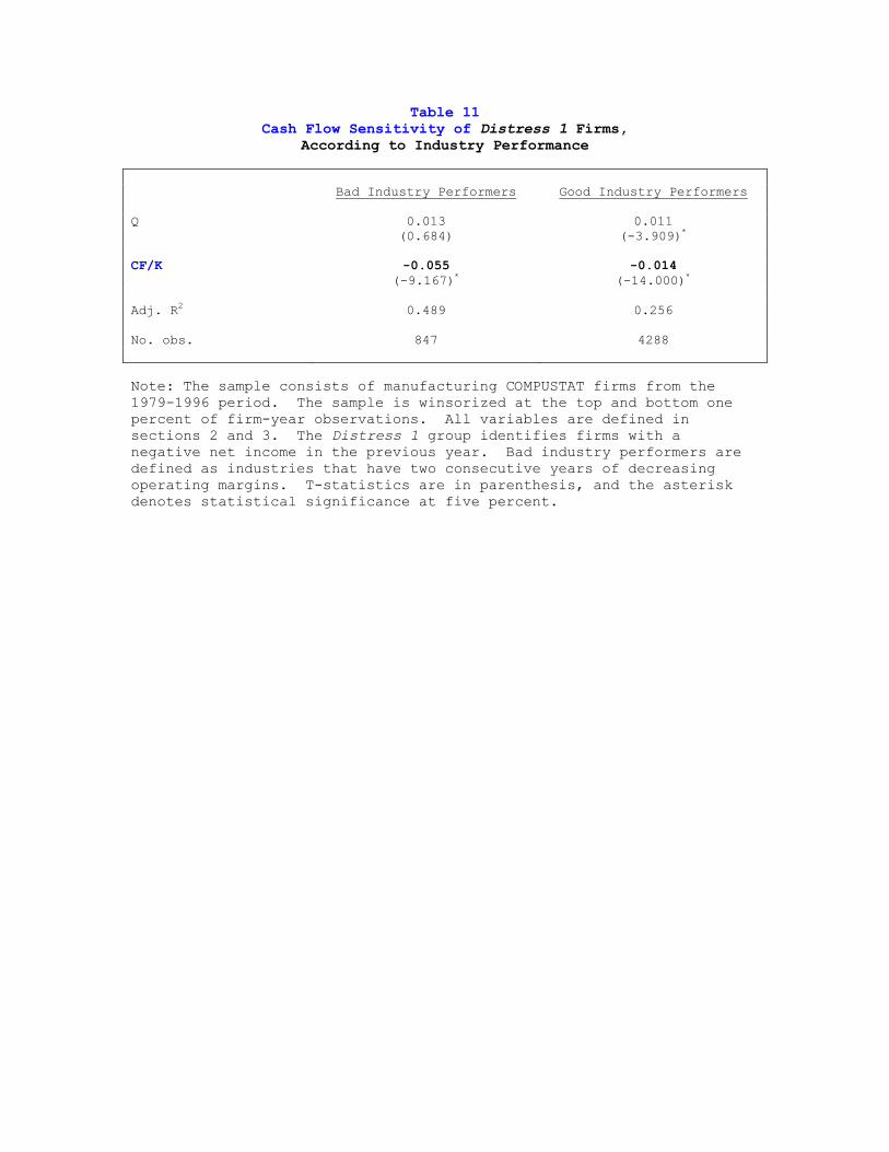
Table 11 Cash Flow Sensitivity of Distress 1 Firms,
According to Industry Performance
Bad Industry Performers Good Industry Performers
Q 0.013 (0.684)
0.011 (-3.909)*
CF/K -0.055
(-9.167)* -0.014
(-14.000)* Adj. R2 0.489
0.256
No. obs. 847 4288
Note: The sample consists of manufacturing COMPUSTAT firms from the 1979-1996 period. The sample is winsorized at the top and bottom one percent of firm-year observations. All variables are defined in sections 2 and 3. The Distress 1 group identifies firms with a negative net income in the previous year. Bad industry performers are defined as industries that have two consecutive years of decreasing operating margins. T-statistics are in parenthesis, and the asterisk denotes statistical significance at five percent.
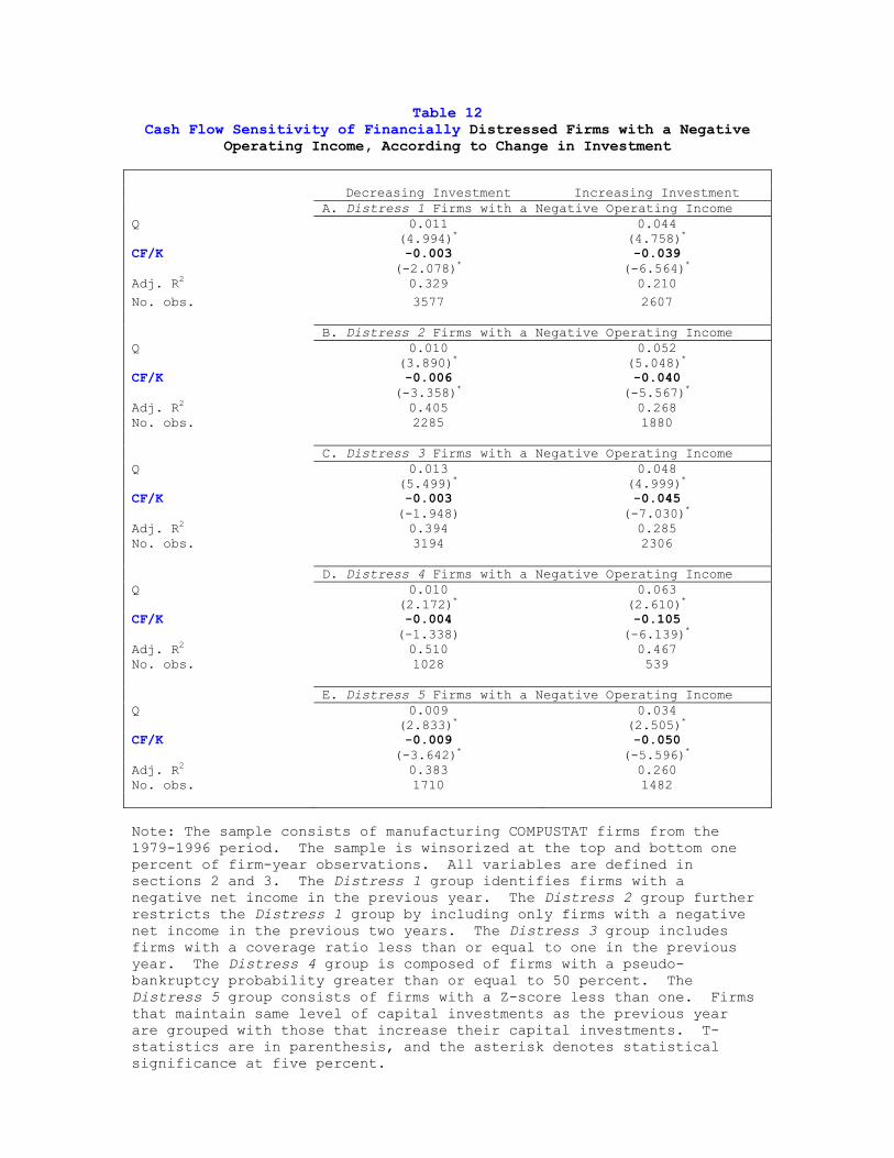
Table 12 Cash Flow Sensitivity of Financially Distressed Firms with a Negative
Operating Income, According to Change in Investment
Decreasing Investment Increasing Investment A. Distress 1 Firms with a Negative Operating Income
Q 0.011 (4.994)*
0.044 (4.758)*
CF/K -0.003 (-2.078)*
-0.039 (-6.564)*
Adj. R2 0.329 0.210 No. obs. 3577 2607 B. Distress 2 Firms with a Negative Operating Income Q 0.010
(3.890)* 0.052
(5.048)* CF/K -0.006
(-3.358)* -0.040
(-5.567)* Adj. R2 0.405 0.268 No. obs. 2285 1880 C. Distress 3 Firms with a Negative Operating Income Q 0.013
(5.499)* 0.048
(4.999)* CF/K -0.003
(-1.948) -0.045
(-7.030)* Adj. R2 0.394 0.285 No. obs. 3194 2306 D. Distress 4 Firms with a Negative Operating Income Q 0.010
(2.172)* 0.063
(2.610)* CF/K -0.004
(-1.338) -0.105
(-6.139)* Adj. R2 0.510 0.467 No. obs. 1028 539 E. Distress 5 Firms with a Negative Operating Income Q 0.009
(2.833)* 0.034
(2.505)* CF/K -0.009
(-3.642)* -0.050
(-5.596)* Adj. R2 0.383 0.260 No. obs. 1710 1482
Note: The sample consists of manufacturing COMPUSTAT firms from the 1979-1996 period. The sample is winsorized at the top and bottom one percent of firm-year observations. All variables are defined in sections 2 and 3. The Distress 1 group identifies firms with a negative net income in the previous year. The Distress 2 group further restricts the Distress 1 group by including only firms with a negative net income in the previous two years. The Distress 3 group includes firms with a coverage ratio less than or equal to one in the previous year. The Distress 4 group is composed of firms with a pseudo-bankruptcy probability greater than or equal to 50 percent. The Distress 5 group consists of firms with a Z-score less than one. Firms that maintain same level of capital investments as the previous year are grouped with those that increase their capital investments. T-statistics are in parenthesis, and the asterisk denotes statistical significance at five percent.
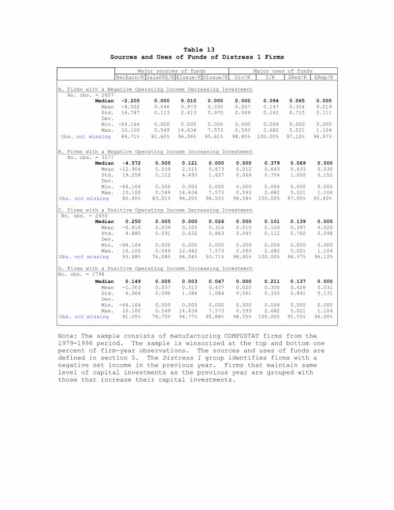
Table 13 Sources and Uses of Funds of Distress 1 Firms
Major sources of funds Major uses of funds
RetEarn/K SalePPE/K EIssue/K DIssue/K Div/K I/K DRed/K ERep/K
A. Firms with a Negative Operating Income Decreasing Investment
No. obs. = 2607 Median -2.200 0.000 0.010 0.000 0.000 0.094 0.065 0.000 Mean -8.002 0.046 0.973 0.335 0.007 0.147 0.304 0.019 Std.
Dev. 14.747 0.113 2.613 0.970 0.049 0.162 0.715 0.111
Min. -64.164 0.000 0.000 0.000 0.000 0.004 0.000 0.000 Max. 10.100 0.549 14.634 7.573 0.593 2.682 5.021 1.104
Obs. not missing 84.71% 81.60% 96.06% 95.61% 98.85% 100.00% 97.12% 94.97%
B. Firms with a Negative Operating Income Increasing Investment No. obs. = 3577
Median -4.572 0.000 0.121 0.000 0.000 0.379 0.069 0.000 Mean -12.904 0.039 2.515 0.673 0.012 0.643 0.433 0.030 Std.
Dev. 19.258 0.112 4.493 1.627 0.069 0.704 1.000 0.152
Min. -64.164 0.000 0.000 0.000 0.000 0.004 0.000 0.000 Max. 10.100 0.549 14.634 7.573 0.593 2.682 5.021 1.104
Obs. not missing 80.40% 83.01% 96.20% 96.55% 98.58% 100.00% 97.05% 93.40%
C. Firms with a Positive Operating Income Decreasing Investment No. obs. = 2450 Median 0.250 0.005 0.000 0.026 0.000 0.101 0.139 0.000 Mean -0.616 0.039 0.105 0.316 0.015 0.126 0.397 0.020 Std.
Dev. 4.880 0.091 0.632 0.863 0.045 0.112 0.760 0.098
Min. -64.164 0.000 0.000 0.000 0.000 0.004 0.000 0.000 Max. 10.100 0.549 12.462 7.573 0.593 2.682 5.021 1.104 Obs. not missing 93.88% 76.08% 96.04% 93.71% 98.45% 100.00% 96.37% 96.12% D. Firms with a Positive Operating Income Increasing Investment No. obs. = 1798
Median 0.149 0.005 0.003 0.047 0.000 0.211 0.137 0.000 Mean -1.303 0.037 0.313 0.437 0.020 0.300 0.426 0.031 Std.
Dev. 6.964 0.090 1.386 1.084 0.061 0.333 0.841 0.131
Min. -64.164 0.000 0.000 0.000 0.000 0.004 0.000 0.000 Max. 10.100 0.549 14.634 7.573 0.593 2.682 5.021 1.104
Obs. not missing 91.05% 76.75% 96.77% 95.88% 98.55% 100.00% 95.55% 96.00%
Note: The sample consists of manufacturing COMPUSTAT firms from the 1979-1996 period. The sample is winsorized at the top and bottom one percent of firm-year observations. The sources and uses of funds are defined in section 5. The Distress 1 group identifies firms with a negative net income in the previous year. Firms that maintain same level of capital investments as the previous year are grouped with those that increase their capital investments.