NBER WORKING PAPER SERIES

INVESTMENT BANKS AS CORPORATE MONITORS IN THE EARLY 20TH CENTURYUNITED STATES

Carola FrydmanEric Hilt

Working Paper 20544http://www.nber.org/papers/w20544

NATIONAL BUREAU OF ECONOMIC RESEARCH1050 Massachusetts Avenue

Cambridge, MA 02138October 2014

An earlier version of this paper circulated under the title "Predators or Watchdogs? Bankers on CorporateBoards in the Age of Finance Capitalism.'' We would like to thank Stanley Engerman, Dan Fetter,Arvind Krishnamurthy, David Matsa, Dimitris Papanikolaou, Joshua Rauh, and Antoinette Schoar,along with participants at the NBER Corporate Finance program meetings, the Economic History Associationannual meetings, and various seminars for helpful comments and suggestions. Richard B. Baker, JackChen, Francis Cho, Hannah Galin, Kimberly Le, Angela Lei, Andrew Marok, Ryan Munoz, ShreySantosh, Sophie Sun, and Veronica Wilson provided excellent research assistance. The views expressedherein are those of the authors and do not necessarily reflect the views of the National Bureau of EconomicResearch.

NBER working papers are circulated for discussion and comment purposes. They have not been peer-reviewed or been subject to the review by the NBER Board of Directors that accompanies officialNBER publications.

© 2014 by Carola Frydman and Eric Hilt. All rights reserved. Short sections of text, not to exceedtwo paragraphs, may be quoted without explicit permission provided that full credit, including © notice,is given to the source.

Investment Banks as Corporate Monitors in the Early 20th Century United StatesCarola Frydman and Eric HiltNBER Working Paper No. 20544October 2014JEL No. N11,N12,N21,N22,N41,N42,N71,N72

ABSTRACT

We use the Clayton Antitrust Act of 1914 to study the effect of bankers on corporate boards in facilitatingaccess to external finance. In the early twentieth century, securities underwriters commonly held directorshipswith American corporations; this was especially true for railroads, which were the largest enterprisesof the era. Section 10 of the Clayton Act prohibited investment bankers from serving on the boardsof railroads for which they underwrote securities. Following the implementation of Section 10 in 1921,we find that railroads that had maintained strong affiliations with their underwriters saw declines intheir valuations, investment rates and leverage ratios, and increases in their costs of external funds.We perform falsification tests using data for industrial corporations, which were not subject to theprohibitions of Section 10, and find no differential effect of relationships with underwriters on thesefirms following 1921. Our results are consistent with the predictions of a simple model of underwriterson corporate boards acting as delegated monitors. Our findings also highlight the potential risks ofunintended consequences from financial regulations.

Carola FrydmanDepartment of EconomicsBoston University270 Bay State RoadBoston, MA 02215and NBERcfrydman@bu.edu

Eric HiltWellesley CollegeDepartment of Economics106 Central StreetWellesley, MA 02481and NBERehilt@wellesley.edu

1 Introduction

Understanding the forces that facilitate firms’ access to external finance is central to the analysis

of the economic growth process. In order to mitigate financial frictions arising from asymmetric

information, firms in many countries around the world often form affiliations with financial inter-

mediaries, which enable the intermediary to gain access to information and monitor management.

However, these affiliations may also be costly for firms: theoretical models suggest that interme-

diaries can use their informational monopoly to hold up firms and charge high interest rates or

fees, thereby distorting the firms’ investments (Sharpe, 1990; Rajan, 1992). The extent to which

financial relationships help or hurt firms is therefore an empirical question. Although a substantial

literature has documented correlations between financial relationships and firm value, convincing

evidence is difficult to obtain, because bank-firm relationships are determined endogenously.

The financial history of the United States offers a unique opportunity to estimate the value of

financial relationships. In the early twentieth century, legal protections of investors were weak, and

asymmetries of information between corporate insiders and outsiders were strong. Perhaps as a

result, close affiliations between public companies and the investment banks that underwrote their

securities, which were the firms’ main source of financing, were quite common. Underwriters often

held seats on their clients’ boards, and they used those positions to participate in their clients’

management and governance. The influence of investment banks in corporate governance gave rise

to fears that financiers were abusing their positions to extract rents from their clients. To restrict

their role in the economy, Section 10 of the Clayton Antitrust Act of 1914 prohibited the securities

underwriters of railroads, which were then the largest and most widely held corporations, from

holding board seats with their clients.

We use Section 10 of the Clayton Act to analyze the value of relationship intermediation.

To address the endogeneity of bank-firm relationships, we exploit the preexisting variation in the

strength of railroads’ relationships with underwriters represented on their boards to estimate the

impact of the imposition of Section 10 on firm outcomes. The results indicate that by restricting

the presence of underwriters on their clients’ boards, the regulation limited the bankers’ role as

monitors and undermined the railroads’ ability to finance valuable investment opportunities.

To motivate our empirical analysis we present a simple illustrative model of underwriters as

1

delegated monitors based on Diamond (1984). Firms choose whether to enter into a relationship

with an underwriter, or to utilize an uninformed banker for their underwriting. Relationship

underwriters have a presence on their clients’ boards, which prevents managers from misreporting

the value of their investments. Such monitoring is costly but it reduces inefficient liquidations,

thereby facilitating access to capital and increasing the efficiency of investments. Larger firms, or

firms with more investment opportunities, are more likely to choose an underwriter-monitor since

they benefit more from avoiding liquidation. For firms that would have selected into a relationship

with an underwriter-monitor, the model predicts that the restrictions imposed by Section 10 would

have led to a decline in market values, investment, and borrowing levels, and would have increased

the cost of external finance.

To test these predictions, we construct a new dataset containing financial information for all

railroads whose shares were listed on the New York Stock Exchange (NYSE) from 1905 to 1929.

We identify the presence of underwriters on the railroads’ boards by matching the names of railroad

directors to the names of the partners and directors of securities underwriters. We also document

the volume of underwriting done by bankers on railroad boards utilizing newly collected evidence

on the underwriting of corporate bonds over this period. To conduct falsification tests, we also

construct a dataset containing the same information for large NYSE-listed industrial firms.

The ideal experiment to measure the effect of relationship intermediation would assign bank-

firm ties randomly. Although bankers and firms endogenously chose to enter into relationships, the

imposition of Section 10 provides a quasi-experiment based on preexisting variation in the degree

of relationship underwriting across firms. Prior to the enactment of the Clayton Act, the average

railroad in our sample had 41% of its securities underwritten by institutions represented on its

board, and this fraction varied considerably across firms. Yet in the year after Section 10 went

into effect, none of the underwriting among our sample railroads was done by banks represented on

their boards. Railroads that had initially maintained stronger relationships with their underwriters

were therefore more severely affected by the regulatory change.

Quite helpful for our analysis, Section 10 was not implemented in 1914, but was repeatedly

postponed by Congress and only went into effect in 1921 when President Wilson vetoed a further

postponement. Thus, its timing is arguably exogenous to firm outcomes, and our findings are

not confounded by the effects of the other antitrust provisions of the Clayton Act, which were

2

implemented in 1914. To comply with the law, underwriters could either resign from the boards

of their client railroads, or retain their directorships and stop providing underwriting services. To

avoid confounding effects from endogenous choices made by firms and banks in anticipation of the

ultimate implementation of Section 10, our empirical framework compares the outcomes of railroads

before and after 1921 by the strength of their affiliations with bankers in 1913 —specifically, the

percent of underwriting done up to 1913 by the banks represented on the railroad’s board in that

year.

We find that railroads with stronger relationships with their underwriters in 1913 experienced

a decline in their investment rates, valuations, and leverage, as well as an increase in their average

interest rates in the years following 1921. For most variables, the economic magnitudes of the

estimates are relatively modest: the effects for the latter three outcomes were equivalent to 2% to

5% of the variables’ 1920 means. However, the effect on investment rates was much larger—a 28%

decline relative to the mean 1920 rate. As a falsification test, we perform the same analysis on

industrial corporations, many of which had strong affiliations with underwriters, but which were

not subject to the prohibitions of Section 10. We find no effects of close ties to underwriters among

those firms, which confirms that the results are not driven by other changes in the role or influence

of investment banks in the 1920s. Thus, relationship underwriting seems to have benefited railroads

by allowing them to finance larger investments at lower costs, thereby improving their valuations.

These findings contrast sharply with the intentions of the authors of the Act, which was to prevent

financiers from expropriating other investors through self-dealing, for example by charging their

client railroads excessive fees for securities issues.

A potential source of concern is that our findings may reflect the selection of particular types of

railroads into close relationships with underwriters. Our estimation framework controls for time-

invariant unobserved firm characteristics, and we use a variety of strategies to deal with selection

on observables. We also address the concern of differential trends for firms with strong relationships

with underwriters by explicitly controlling for such trends. Moreover, we create a placebo “Clayton

Act” in the year 1909, and find no differential effects of the strength of underwriting relationships

following that year.

The prohibitions of Section 10 went beyond securities underwriting, raising the concern that

our results could be driven by changes unrelated to the disruption of bank-firm relationships.

3

In particular Section 10 prohibited other forms of self-dealing by railroad directors, such as the

purchasing of inputs from affiliated firms. However, our results are robust to including controls for

board interlocks with industrial firms that were likely suppliers of capital equipment to railroads.

The authors of the Act also intended it to limit the ability of banker-directors to facilitate collusion

among competing railroads. An additional source of concern regarding our results could be that

they reflect the impact of dissolutions of board interlocks among competing railroads following the

resignations of bankers who held multiple railroad directorships. Yet we show that our results are

not driven by the preexisting level of director interlocks with competitors created by underwriters.

These findings further suggest that the main mechanism behind the effects we estimate is the

disruption of the role of underwriters as monitors.

Finally, we use an instrumental variables framework to analyze the changes made to bank-

firm relationships prior to 1921, in anticipation of Section 10’s eventual implementation. The

results obtained from an OLS specification that estimates the effect of bank-firm relationships in

1920 (rather than 1913) on firm outcomes after 1921 are biased by the endogenous changes in

banker directorships made in anticipation of the implementation of Section 10. We find that IV

estimates of the same specification are larger than the OLS estimates, suggesting that bankers

stepped down from the boards of railroads that suffered the most from financial constraints in

anticipation of the implementation of the regulation, perhaps because those firms were more likely

to require underwriting services in the future. These results also suggest that our estimation

strategy, which utilizes the preexisting variation in strength of bank-firm relationships in 1913,

leads us to underestimate the effect of bank monitoring in relaxing financial constraints in our

main results.

Our analysis contributes to a substantial literature assessing whether relationship banking is

beneficial or detrimental for firms. This question has been studied using modern data from coun-

tries characterized by bank-centered financial systems, such as Germany (Gorton and Schmid, 2000;

Agarwal and Elston, 2001) and Japan (Weinstein and Yafeh, 1998; Morck and Nakamura 1999), and

where bankers have only a modest presence on firms’ boards, such as the United States (Booth and

Deli, 1999; Kroszner and Strahan, 2001; Guner, Malmendier and Tate, 2007). Economic historians

have also investigated the effect of ties to J.P. Morgan & Co. on the value and investments of Amer-

ican corporations in the early twentieth century (DeLong, 1991; Ramirez, 1995; and Cantillo Simon

4

1998) and the value of ties to financial intermediaries in other countries (Fohlin, 1998; Guinnane,

2002; Braggion and Ongena, 2014). These studies, however, generally do not address the endogene-

ity of affiliations between firms and banks.1 We add to this literature by exploiting a regulatory

change that generates exogenous variation on the strength of the relationship between underwriters

and their clients, and therefore makes it possible to identify the effects of these associations on a

variety of firm outcomes.

More generally, our paper contributes to the analysis of the effect of board composition on

firm outcomes. This has long been a central question in the study of corporate governance, but

the empirical literature has only recently begun to address the challenges posed by the endogenous

choice of board members (Hermalin and Weisbach, 1988; 1998; 2003). Thus far, only two regulatory

changes have been used to address this problem. First, a handful of papers study the introduction

of gender quotas in Norway in 2006 on firm values (Ahern and Dittmar, 2012; Nygaard, 2011) and

labor decisions (Matsa and Miller, 2013). However, it is not clear how or why gender composition

should affect firm governance. Duchin, Matsusaka and Ozbas (2010) investigate the role of inde-

pendent directors, which the theoretical literature has argued can benefit or hurt firms (see Adams,

Hermalin and Weisbach, 2010, for a review). Exploiting mandates to appoint outside directors to

corporate boards, the authors find that the effects of director independence on firm performance

depends on the cost of information acquisition. Our paper adds to this literature by focusing on

an important and controversial aspect of corporate governance: the role of bankers on boards,

and their ability to monitor their client firms. In addition to studying the effect of relationship

underwriting on firm value, we also consider its impact on other important firm outcomes, such as

access to credit and investments.

Finally, the analysis of this paper also relates to the literature addressing how regulations have

restricted the role of financial institutions in the American economy over time (see, for example,

Roe 1994). A distinctive characteristic of the governance of American corporations today is the

relatively minor presence of financial institutions on the boards of nonfinancial firms (Kroszner

1There are two main exceptions to this criticism. Cantillo Simon (1998) analyzes the stock returns of the firmsfrom which the partners of J.P. Morgan & Co. voluntarily resigned in early 1914. However, our instrumentalvariables analysis suggests that voluntary resignations made prior to the implementation of Section 10 were based onprivate information on the quality of firms. This suggests that the results of Cantillo Simon may confound selectioneffects with the pure impact of banker-directors on firm value. Guner, Malmendier and Tate (2007) use instrumentalvariables to address the endogenous presence of commercial bankers on the boards of American firms in the 1990s.We contrast their findings to ours in the conclusion.

5

and Strahan, 2001; Guner, Malmendier and Tate 2008). But investment banks played a major

role in the governance of corporations merely a century ago.2 Our paper suggests that regulations

designed to restrain the presence of bankers on boards may have been one contributing factor to

the decline in the role of financial institutions in American corporate governance.

Our findings also highlight the potential risks of unintended consequences from financial regu-

lations: the Clayton Act’s restrictions on the role of financiers in the governance of railroads ended

up harming the firms they were intended to help. We return to this point in the conclusions of the

paper.

2 Historical Background: Railroads, Investment Banks, and the

Clayton Act

2.1 Underwriters and railroad governance

The second half of the nineteenth century witnessed the emergence of major railroad systems in the

United States, which quickly became the largest business enterprises in the American economy.3

At that time, the weak legal protections available for minority investors failed to constrain the

behavior of controlling insiders, and asymmetries of information between those insiders and outside

investors were acute (Hilt, 2014). That era of “ruthless and criminal abuse of power” by controlling

shareholders was plagued by scandals, which repeatedly shook the confidence of outside investors in

railroad securities.4 In reaction, the investment bankers who facilitated the distribution of railroad

bonds sought a more active role in their governance.

At the time, state regulations constrained commercial banks to be relatively small, and those

institutions were therefore unable to provide loans of the size required to satisfy the railroads’

large demand for external financing.5 Instead, railroads financed their growth primarily by issuing

2On the historical role of investment banks, see Carosso, 1970; Carosso and Sylla, 2001; Morrison and Wilhelm,2007; Hannah 2011; and Flandreau and Flores, 2012. Our paper adds to this literature by providing the firstcomprehensive documentation of the representation of underwriters on the boards of major corporations in the earlytwentieth century.

3In 1870 the capitalization of just one of the largest railroads was equal to 40 percent of the combined capitalizationof all manufacturing corporations listed on the Boston Stock Exchange, where the major industrial firms were listedat that time.

4Moulton (1933:7). Colorful examples of these scandals can be found in Adams and Adams (1871), Campbell(1938) and White (2012).

5In the nineteenth and early twentieth centuries, commercial banks were generally prohibited from branching,

6

bonds. A small number of American investment banks developed the capacity to underwrite these

large debt issues; their critical role in the distribution of railroad securities gave them influence

over their clients. Particularly after the financial panic of 1893 and the resulting wave of railroad

bankruptcies, major securities underwriters, which at the time included private partnerships, trust

companies, and affiliates of commercial banks, began to hold board seats with their client railroads,

and monitor the activities of their managers (Carosso, 1970; Martin, 1971).

In this era of “relationship underwriting,” the interests of underwriters were well aligned with

those of railroad securities holders. In most underwriting transactions the bankers typically pur-

chased the issue from a railroad and re-sold it at a premium, bearing market placement risk. More-

over, future revelations of mismanagement or fraud by the railroad damaged the underwriter’s

reputation among investors, and hurt its capacity to distribute future issues. Thus, underwriters

had strong incentives to monitor or even control their clients. A clear illustration of the relationship

between bankers and management is found in a well-known confrontation between the management

of a railroad and J.P. Morgan. The management argued that they shouldn’t have been expected

to submit control over their railroad to Morgan. Morgan replied “Your railroads! Your railroads

belong to my clients.”6

The banks represented on a railroad’s board often led the underwriting syndicates for the firm’s

debt issues. Using novel data on the underwriting of securities, we find that the closest affiliations

tended to be between the largest railroads and top-ranking investment banks. These relationships

were often long-lasting, and enabled the underwriters to gain access to private information about the

railroad, and exert influence over management. However, the representation of investment bankers

on railroad boards was nearly ubiquitous, and in some cases board seats were not accompanied by an

underwriting relationship. These latter banker-directors may simply have been sought as financial

experts, and may have served on the board in the hope of becoming a provider of underwriting

services in the future (see, for example, Cohan, 2011). The early twentieth century was thus known

as the era of “banker control” of railroads.7

and were required to confine their operations to a single office. Calomiris (1995) analyzes the consequences of theserestrictions.

6Wall Street Journal 1 April 1913. In the original, the speakers use the abbreviated term “road” rather than“railroad”; we have changed the text to reflect modern usage.

7However, the term “banker” was often understood to mean “anyone who had made a fortune in financial deal-ings” (Martin 1971: 18) and therefore also denoted those who would be described today as “corporate raiders” orspeculators—agents whose interests and incentives were quite different from those of securities underwriters. Instances

7

Over time, the role of underwriters in the governance of railroads and other major corporations

became subject to political criticism. By the first decade of the twentieth century, a small number

of elite financial institutions held directorships with the majority of large corporations, which

aroused anti-banker sentiment, particularly following the Panic of 1907.8 In 1912, the US House of

Representatives authorized an investigation of the so-called “money trust” by a committee headed

by Representative Arsene P. Pujo (Pujo Committee, 1913a, 1913b). Financiers were accused of

controlling the firms’ access to credit, and using their power to enrich themselves at the expense of

the public in numerous ways, such as charging their clients high interest rates or fees for securities

issues, facilitating collusion, and tunneling resources to other firms under their control (see Brandeis,

1914).

Financiers defended themselves during the Pujo investigation utilizing arguments that are con-

sistent with their role as corporate monitors. They claimed that their presence on boards allowed

them to supervise their clients, and helped to assure investors that the company was well man-

aged. Their clients could issue securities on more favorable terms with their representation because

investors valued the banks’ reputation, which in turn gave underwriters incentives to effectively

monitor them (Carosso, 1970; DeLong, 1991). Indeed, guides for investors from the era suggested

that the participation of a leading underwriter in the management of a railroad enhanced the value

of its securities (see, for example, Sakolski, 1913:51).

Ultimately, the Pujo Committe’s report called for Congress to enact regulations on the role of

financiers in the economy (Pujo Committee, 1913b). In an effort to forestall such regulation, the

partners of the most important investment bank, J.P. Morgan & Company, announced they would

resign from 30 boards at the beginning of January 1914.9

2.2 The Clayton Act of 1914

Those resignations, however, did not deter efforts to impose new regulations on bankers. Inspired

by the findings of the Pujo Committee, in January 1914 President Woodrow Wilson gave a special

of “banker management” in which securities underwriters in fact had little influence were criticized as producing firmssuffering from “financial weakness,” and operating “for the benefit of insiders” (Ripley, 1915: 525).

8On the role of financial intermediaries during this panic, see Frydman, Hilt and Zhou (forthcoming). On theearly history and political complexity of anti-banker political sentiment, see Hammond (1957).

9See “Morgan Firm Out From Thirty Boards,” and “May Modify Legislation: Concessions by Financiers Likelyto Stop Radical Action by Congress,”New York Times, 3 January 1914. See also Cantillo Simon (1998).

8

address to Congress calling for new antitrust legislation. The address repeatedly mentioned the

role of bankers in corporate governance, particularly in the case of railroads, and argued that

those who direct public affairs now recognize...the great harm and injustice that hasbeen done to many, if not all, of the great railroad systems of this country by the wayin which they have been financed and their own distinctive interests subordinated tothe interests of the men who financed them...(Wilson 1914, vol 29, p. 155).

In October 1914, Congress passed the Clayton Antitrust Act. Besides its many clauses intended

to clarify and strengthen the Sherman Antitrust Act of 1890, the Clayton Act included several

provisions designed to limit the power of the money trust in specific industries. Section 10 explicitly

prohibited transactions between railroads and firms with which they had a director or executive in

common. In particular, it forbade railroads from having “dealings in securities” with any financial

institution that had a partner or director on the railroads’ board.10 The act also outlawed other

forms of self-dealing by directors; we discuss the effects of these broader prohibitions in detail in

Section 5.5 below.

Importantly, the rule did not prohibit financiers from sitting on railroad boards, but it forbade

banks that held railroad board seats from underwriting securities for that railroad. Bankers who

sat on the boards of railroads could choose to remain on those boards and cease to act as their

underwriters, or they could continue to underwrite securities for the railroads, and resign from their

boards. We therefore design our empirical strategy appropriately not to confound the estimates of

the effects of the regulatory change on firm outcomes with the endogenous choice of underwriters

of whether to step down from corporate boards.

The implementation of Section 10 of the Clayton Act did not occur immediately, however. A

two-year delay in its implementation was enacted, so that the Interstate Commerce Commission

(ICC) could develop the capacity to enforce it (see House Judiciary Committee, 1917). Further

such delays were then implemented in 1916 and 1918.11 The railroads strenuously argued against

the implementation of Section 10, stating that they “ought not to be required to elect whether or

10Oct. 15, 1914, ch. 323, 38 Stat. 730. (After lobbying by the railroads, this term was repealed in 1988.)11The effects of World War I severely disrupted the operations of American railroads, and strengthened their

arguments for a delay. In 1917, the federal government assumed control over the industry, leasing the railroads’assets in exchange for a guaranteed rate of return based on historical averages. Federal control, which was welcomedby the industry, suspended many railroad regulations and coordinated the operations of individual firms to serve theneeds of the war effort. Control was restored to the railroads themselves in March 1, 1920.

9

not they will cut themselves off from sources of money supply or will leave off of their boards some

of their strongest directors” (New York Central Railroad, 1921: 16). Although Congress passed

a one-year delay in 1920, President Wilson vetoed it on December 30, 1920, and Section 10 went

into effect on January 1, 1921. Thus, the timing of the implementation of the reform was generally

unexpected, and exogenous to firm outcomes. Importantly, our empirical findings presented in

Section 5 are not confounded by all other antitrust provisions of the Clayton Act, which were

implemented in 1914.

2.3 Effects of Section 10 on Bank-Firm Relationships

We begin our analysis of the effects of Section 10 by documenting the impact of the regulation

on railroads’ relationships with their underwriters. The extent to which Section 10 was actually

obeyed is explored in Figure 1, which presents a three-year moving average of the percentage of debt

underwritten by investment banks represented on the boards of the sample railroads and industrial

firms, from 1907-1929.12 The figure indicates that prior to 1913, around 60 percent of railroad

and industrial firm debt was underwritten by bankers with board representation. Following 1914,

when the Clayton Act was passed, the ratio began to decline for railroads, reaching a level of 35

percent by 1920, whereas the level for industrials remained roughly stable. Finally, following the

implementation of Section 10 in 1921 underwriting by bankers on railroad boards fell to almost zero

(the moving average of the figure obscures the fall to zero in 1921 and near-zero in the following

years).13 In contrast, there is no equivalent shift in underwriting by bankers on the boards of

industrials, which were not subject to Section 10, indicating that the change among railroads was

in fact due to that statute.

Section 10 of the Clayton Act did not actually mandate that underwriters step down from

boards; banker-directors could comply by ceasing to provide underwriting services. However, many

railroads and underwriters apparently concluded that the optimal response was for the banker to

resign. The resignations of prominent bankers from major railroads’ boards in the months following

12The greater volatility in the case of industrials is due to the much lower volume of bond underwriting amongthose firms. See the Appendix.

13There is little research on the enforcement or judicial interpretation of Section 10 (one exception is William &Mary Law Review, Note, 1976). However, Figure 1 suggests that in the late 1920s compliance with the law was goodbut not always perfect. If firms were able to circumvent the law to some extent, this should bias our frameworkagainst finding an effect.

10

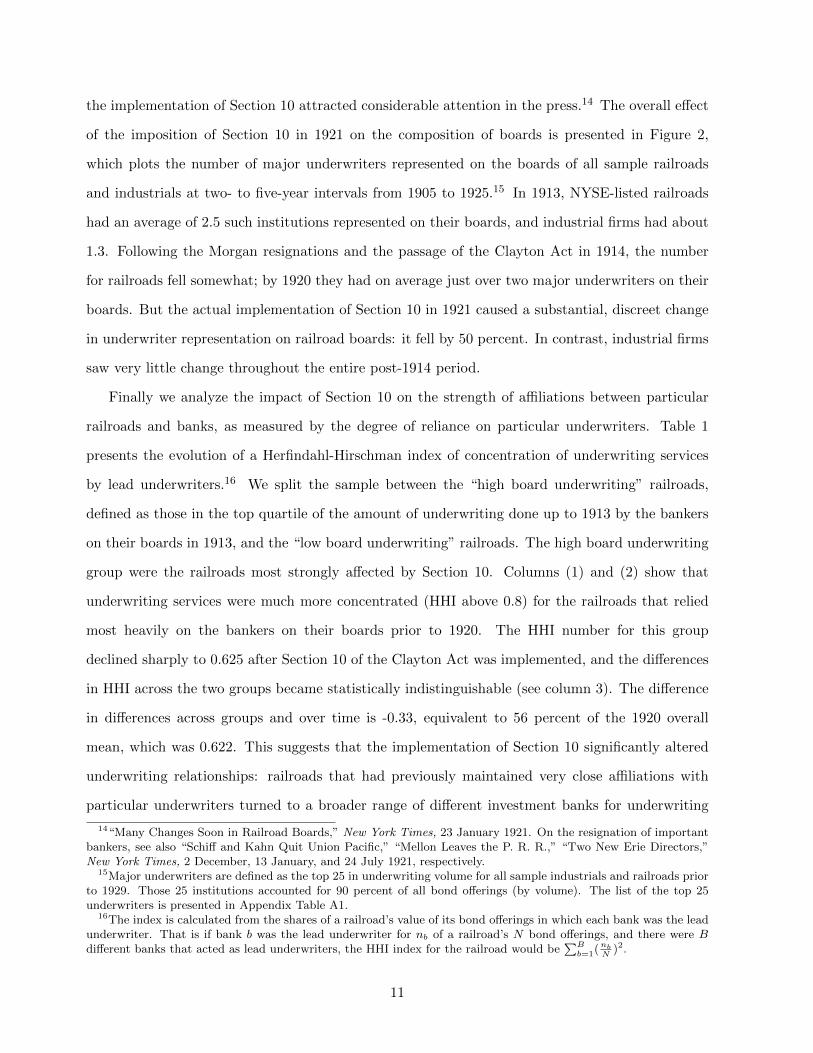
the implementation of Section 10 attracted considerable attention in the press.14 The overall effect

of the imposition of Section 10 in 1921 on the composition of boards is presented in Figure 2,

which plots the number of major underwriters represented on the boards of all sample railroads

and industrials at two- to five-year intervals from 1905 to 1925.15 In 1913, NYSE-listed railroads

had an average of 2.5 such institutions represented on their boards, and industrial firms had about

1.3. Following the Morgan resignations and the passage of the Clayton Act in 1914, the number

for railroads fell somewhat; by 1920 they had on average just over two major underwriters on their

boards. But the actual implementation of Section 10 in 1921 caused a substantial, discreet change

in underwriter representation on railroad boards: it fell by 50 percent. In contrast, industrial firms

saw very little change throughout the entire post-1914 period.

Finally we analyze the impact of Section 10 on the strength of affiliations between particular

railroads and banks, as measured by the degree of reliance on particular underwriters. Table 1

presents the evolution of a Herfindahl-Hirschman index of concentration of underwriting services

by lead underwriters.16 We split the sample between the “high board underwriting” railroads,

defined as those in the top quartile of the amount of underwriting done up to 1913 by the bankers

on their boards in 1913, and the “low board underwriting” railroads. The high board underwriting

group were the railroads most strongly affected by Section 10. Columns (1) and (2) show that

underwriting services were much more concentrated (HHI above 0.8) for the railroads that relied

most heavily on the bankers on their boards prior to 1920. The HHI number for this group

declined sharply to 0.625 after Section 10 of the Clayton Act was implemented, and the differences

in HHI across the two groups became statistically indistinguishable (see column 3). The difference

in differences across groups and over time is -0.33, equivalent to 56 percent of the 1920 overall

mean, which was 0.622. This suggests that the implementation of Section 10 significantly altered

underwriting relationships: railroads that had previously maintained very close affiliations with

particular underwriters turned to a broader range of different investment banks for underwriting

14“Many Changes Soon in Railroad Boards,” New York Times, 23 January 1921. On the resignation of importantbankers, see also “Schiff and Kahn Quit Union Pacific,” “Mellon Leaves the P. R. R.,” “Two New Erie Directors,”New York Times, 2 December, 13 January, and 24 July 1921, respectively.

15Major underwriters are defined as the top 25 in underwriting volume for all sample industrials and railroads priorto 1929. Those 25 institutions accounted for 90 percent of all bond offerings (by volume). The list of the top 25underwriters is presented in Appendix Table A1.

16The index is calculated from the shares of a railroad’s value of its bond offerings in which each bank was the leadunderwriter. That is if bank b was the lead underwriter for nb of a railroad’s N bond offerings, and there were Bdifferent banks that acted as lead underwriters, the HHI index for the railroad would be

∑Bb=1(nb

N)2.

11

services once those intermediaries could no longer have a presence on their clients’ boards.

3 Theoretical framework

Restricting relationships between firms and underwriters can have different effects on firms. If

underwriting relationships relax firms’ financial constraints, then severing or disrupting those re-

lationships may be costly to firms. On the other hand, if relationships enable underwriters to

extract rents, the restriction may free firms from those costs. The authors of the Clayton Act were

animated by concerns over the latter, and gave little consideration to the former.

To motivate our empirical analysis, we present a simple theoretical framework that models the

decision to utilize an underwriter who can effectively monitor the firm, and produces a series of

predictions regarding the effects of the implementation of Section 10 on specific firm outcomes.

We model underwriters with board seats as delegated monitors, in the spirit of Diamond (1984).

Instead of focusing on relationship lending, which is more common in the literature, our emphasis

is on relationship underwriting. In the early twentieth century, railroads relied mostly on bond

finance and, as we discussed above, underwriters had strong incentives to monitor their clients.

Our model takes as given the need to issue bonds to finance new investments, and emphasizes the

potential of underwriters to monitor management.

The key friction in the model arises from an information asymmetry: a firm’s insiders observe

the cash flows it generates, but its providers of external financing, the bondholders, do not. As

in Diamond (1984), this creates a moral hazard problem, since the insiders will be tempted to

underreport cash flows and reduce the payout to the bondholders, keeping the residual for them-

selves. The bondholders use the threat of costly liquidation to induce truthful revelation of the

value of the cash flows, which raises the cost of debt, and reduces the range of investments that can

get financed. In our setting, the investment bank that underwrites a firm’s debt can potentially

alleviate these problems by monitoring the firm on behalf of the bondholders. If underwriters with

board seats can gain access to the firms’ private information, and if they can commit to reporting

this information to the bondholders, the asymmetric information problem is resolved. On the other

hand, monitoring is costly and the underwriter will charge a fee for this service, which may be

prohibitively expensive for some firms.

12

3.1 Setup

The model has two periods. There is a continuum of firms f , which differ at time 0 in the probability

λf ∼ F (λ) of having access to an investment opportunity at time 1. The probability λf can be

thought as the firm’s growth opportunities or its size.17

An investment opportunity requires an outlay of 1 unit of capital in period 1, and yields a

stochastic payoff in period 2. Projects vary ex-ante in their quality p: with probability p the

project is successful and its cash flows are worth VH , with probability 1 − p the project is only

worth VL < VH . For simplicity, we assume that p is observable and verifiable by all parties, and that

p is distributed U [0, 1] and independent across firms. The realization of VH or VL is observed only

by the firm’s insiders, who will therefore be tempted to report VL to outside investors regardless of

the true realization, and keep any additional cash flows for themselves.

If a project arrives in period 1, it must be financed by the issuance of debt, and the firm needs

a banker to underwrite these securities. The underwriter sells the debt to risk-neutral investors,

who have a required expected rate of return equal to R ∈ (VL, VH).

At time 0, prior to the arrival of an investment opportunity, firms decide the type of underwriter

that will market its securities. Specifically, they choose whether or not to offer a board seat to an

underwriter. If an underwriter has a seat on the firm’s board, they can monitor the firm and verify

the true value of the project’s payoff, VL or VH . If there is no banker on the firm’s board, then the

firm must use an arms-length underwriter who cannot monitor the firm. For simplicity, we assume

that the underwriters receive no fee for marketing securities, but that they are compensated for

providing monitoring services in the form of a fee of M .18

We denote F the face value of the debt issued by the firm, which is sold for a price of 1. At

time 2, bondholders can choose to liquidate the project, in which case they only recover an amount

L < VL, and the insiders receive a payoff of 0.

With an arm’s-length underwriter, outside investors anticipate that insiders have an incentive to

17Although for simplicity our framework is static, in a dynamic setup firms with higher λf would acquire moreprojects over time, and therefore be larger in equilibrium.

18Effectively, we assume a zero marginal cost of exerting monitoring effort if there is a banker on board, and infiniteotherwise. Our model can be extended to allow for the monitoring fee to depend on the arrival of an investmentopportunity. As long as there is a fixed component to this fee—that is, the monitoring fee is not purely proportionalto λf—larger firms will choose to have a monitor. Note that if the fee was exactly proportional to the probability ofreceiving a project, there would be no selection of firms into monitoring relationships based on their ex-ante growthopportunities: either all firms would choose to have bankers on boards, or no one would.

13

lie about the payoff of the project. To guarantee truth-telling by the insiders, investors will always

liquidate the firm if the insiders report that the payoff is VL.19 Since investors will therefore receive

L in the low state and require an expected rate of return R to invest in the firm, the payment in

the good state (and therefore the maximum amount that the firm can borrow) is given by:

FN (p) =R− (1− p)L

p(1)

Since the firm’s insiders will only take on an investment opportunity with positive expected payoffs,

investment will take place as long as p (VH − FN ) ≥ 0, or

p ≥ p∗ ≡ R− LVH − L

(2)

If instead the firm uses an investment bank with a board seat to underwrite their debt, the bank

will learn the true value of the project’s payoff and report it to the bondholders, who no longer

have incentives to liquidate the firm when VL is reported. As a result, the amount that the firm

must promise to repay outside investors in the good state becomes:

FM (p) =R− (1− p)VL

p(3)

Thus, investment will occur for a project p as long as

p ≥ p ≡ R− VLVH − VL

(4)

A comparison of (2) with (4) reveals that p∗ > p. Thus, the lack of monitoring leads to under-

investment: positive NPV projects p ∈ [p, p∗) cannot be financed in the case of arm’s-length under-

writing. This distortion occurs because the costs of raising external funds under non-monitoring

are higher, as investors need to be promised a higher amount relative to the efficient case (FN (p) >

FM (p)).

Having a banker on the board who can potentially act as a monitor is costly, and results in a loss

of value to the firm’s insiders equal to M . By incurring this cost at t = 0, the firm has the option

19We assume that investors can commit to this liquidation strategy ex-ante.

14

of using this banker to underwrite its securities if it needs external funds. Even though we refer to

M as monitoring costs, these costs include not only the direct fees paid to the underwriter-monitor

but also other indirect costs associated with having bankers on boards, likely including rents that

bankers may extract from the firm, as the Progressives argued during the Pujo Committee hearings.

Thus, these “monitoring fees” could potentially amount to a substantial fraction of firm value.

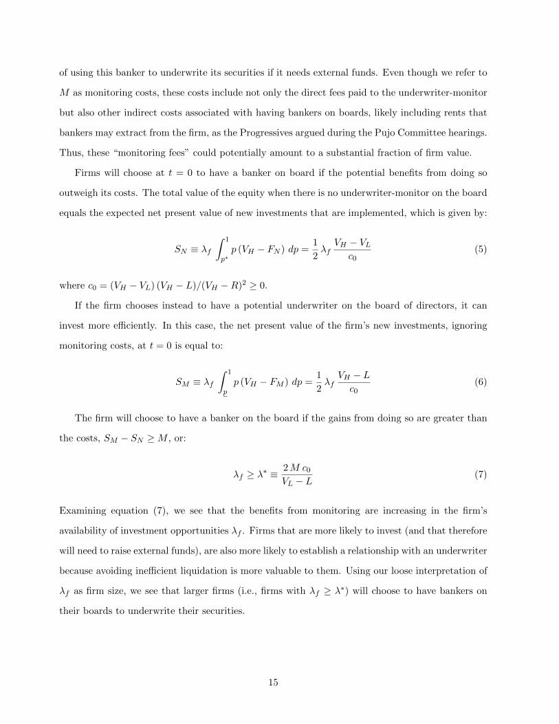
Firms will choose at t = 0 to have a banker on board if the potential benefits from doing so

outweigh its costs. The total value of the equity when there is no underwriter-monitor on the board

equals the expected net present value of new investments that are implemented, which is given by:

SN ≡ λf∫ 1

p∗p (VH − FN ) dp =

1

2λf

VH − VLc0

(5)

where c0 = (VH − VL) (VH − L)/(VH −R)2 ≥ 0.

If the firm chooses instead to have a potential underwriter on the board of directors, it can

invest more efficiently. In this case, the net present value of the firm’s new investments, ignoring

monitoring costs, at t = 0 is equal to:

SM ≡ λf∫ 1

pp (VH − FM ) dp =

1

2λf

VH − Lc0

(6)

The firm will choose to have a banker on the board if the gains from doing so are greater than

the costs, SM − SN ≥M , or:

λf ≥ λ∗ ≡2M c0

VL − L(7)

Examining equation (7), we see that the benefits from monitoring are increasing in the firm’s

availability of investment opportunities λf . Firms that are more likely to invest (and that therefore

will need to raise external funds), are also more likely to establish a relationship with an underwriter

because avoiding inefficient liquidation is more valuable to them. Using our loose interpretation of

λf as firm size, we see that larger firms (i.e., firms with λf ≥ λ∗) will choose to have bankers on

their boards to underwrite their securities.

15

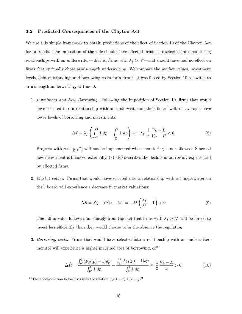
3.2 Predicted Consequences of the Clayton Act

We use this simple framework to obtain predictions of the effect of Section 10 of the Clayton Act

for railroads. The imposition of the rule should have affected firms that selected into monitoring

relationships with an underwriter—that is, firms with λf > λ∗—and should have had no effect on

firms that optimally chose arm’s-length underwriting. We compare the market values, investment

levels, debt outstanding, and borrowing costs for a firm that was forced by Section 10 to switch to

arm’s-length underwriting, at time 0.

1. Investment and New Borrowing. Following the imposition of Section 10, firms that would

have selected into a relationship with an underwriter on their board will, on average, have

lower levels of borrowing and investments.

∆I = λf

(∫ 1

p∗1 dp−

∫ 1

p1 dp

)= −λf

1

c0

VL − LVH −R

< 0, (8)

Projects with p ∈ (p, p∗) will not be implemented when monitoring is not allowed. Since all

new investment is financed externally, (8) also describes the decline in borrowing experienced

by affected firms.

2. Market values. Firms that would have selected into a relationship with an underwriter on

their board will experience a decrease in market valuations:

∆S = SN − (SM −M) = −M(λfλ∗− 1

)< 0. (9)

The fall in value follows immediately from the fact that firms with λf ≥ λ∗ will be forced to

invest less efficiently than they would choose to in the absence the regulation.

3. Borrowing costs. Firms that would have selected into a relationship with an underwriter-

monitor will experience a higher marginal cost of borrowing, or20

∆R =

∫ 1p∗(FN (p)− 1)dp∫ 1

p∗ 1 dp−

∫ 1p (FM (p)− 1)dp∫ 1

p 1 dp≈ 1

2

VL − Lc0

> 0, (10)

20The approximation below uses uses the relation log(1 + x) ≈ x− 12x2.

16

where the total amount of interest paid R = F −1 is the difference between the the face value

of the debt issued by the firm and the amount it borrowed.21

Note that in our model, the book value of assets at t = 0 is independent of the type of under-

writer. Thus, these predicted changes in the level of investment, new borrowing, and market values

are also applicable to investment rates, leverage ratios, and Tobin’s Q. This simple framework

therefore predicts that the railroads with a stronger preexisting association with their underwriters

through their boards would experience a decline in values, investment rates and leverage, and an

increase in their borrowing costs as a consequence of the implementation of Section 10.

3.3 Discussion of the model’s assumptions and implications

In our framework, firms with more investment opportunities are more likely to enter into a relation-

ship with an underwriter on their board. This feature is consistent with a fact we document below,

that close affiliations between railroads and underwriters were most frequently established among

the largest and best-known railroads, which suggests that adverse selection motives for establishing

a relationship—such as screening or certification—were less likely to have played an important role

in corporate debt markets at that time.22

The friction at the heart of the model, that only insiders can observe the true state of the

firm’s cash flows, seems consistent with the history of the railroad industry, which is replete with

examples of the condition of firms being “sedulously hidden” from investors as insiders engaged

in “plundering” (Campbell, 1938: 92). That bankers with board seats could get access to this

hidden information, and that they often restricted management from engaging in value-destroying

behavior, is also well supported by the history.23

21The marginal interest rate paid by firms when the Clayton Act restriction is enforced is affected by two forces.First, for a given project of quality p, firms will pay a higher interest rate when the underwriter is not allowed tomonitor. This direct effect will increase interest expenses for the affected firms. However, there is also an indirecteffect due to project selection: under the Act’s restriction, firms will pass up on marginal investment opportunities(that is, projects with p ∈ (p, p∗)). Since these investments are ex-ante riskier, this second force will tend to reducethe interest expense paid by firms. In our setup, the first effect dominates.

22On the certification role of underwriters more generally, see Booth and Smith (1986) and Chemmanur andFulghieri (1994).

23For example, when J.P. Morgan took a seat on the board of the Northern Pacific Railroad in 1883, he found thatthe expenses for construction and equipment had vastly exceeded the estimated costs, and that Villard, the Presidentof the company, had liberally spent funds on various other projects. The railroad quickly fell into financial trouble,and Morgan restored the credit and earnings of the firm by reorganizing its financing, appointing a strong committeeto oversee the activities of the firm, and encouraging Villard to resign (Strouse, 1999). Other such examples arepresented in Campbell (1938).

17

In our simple framework, we have assumed that underwriters with board seats can commit

ex-ante to monitor and reveal the true state of firms to investors. We make this assumption for

simplicity; in its absence, there will be no underwriter-monitors in equilibrium in our static model.24

(In multi-period settings, incentives to monitor can be sustained by the fear of loss of reputation;

see Boot (2000) for a survey.) An alternative interpretation of our framework that does not require

this assumption is that informed underwriters can smooth the bankruptcy process and avoid costly

liquidation. In this formulation, an underwriter on the board can help creditors recover the full

value of the assets VL in the event of default. Indeed, anecdotal evidence suggests that established

relationships with financial intermediaries was particularly helpful during corporate reorganizations

(Daggett, 1908; Dewing, 1914). When railroads defaulted on their debts, the bondholders often

promoted the underwriters of those securities to represent them in the receivership committees.

Perhaps due to their privileged access to the financial information, these bankers played an instru-

mental role in restructuring the liabilities, thereby ensuring a prompt reorganization of the firms’

capital structures, and avoiding liquidation.

Finally, theoretical work has argued that a potential cost from relationship intermediation is

that banks may use their informational monopoly to hold up the firm and charge ex-post high

interest rates or fees (Sharpe, 1990; Rajan, 1992). In our model, this potential rent extraction is

embodied in the cost M . But since firms freely (and optimally) select into a relationship with an

underwriter, banks can extract these rents only as long as they do not exceed the benefits to the

firm from entering into a relationship. Contemporary critics’ arguments that the monopolization

of credit markets was so extreme that firms had little choice but to submit to banker control were

not consistent with this assumption (Brandeis, 1914). But if those critics were correct, we would

expect the implementation of Section 10 to have the opposite effects on market value and borrowing

costs than those predicted in the monitoring model: the value of the firms should have risen and

interest rates should have fallen as railroads escaped the monopolistic grip of underwriters. The

effect on borrowing and investment levels is potentially ambiguous; as in the monitoring model,

leverage and investment rates may have fallen following 1920 if the banker-directors had forced their

clients to borrow greater amounts in order to finance inefficient projects prior to the regulation. In

24If monitoring entails some costs to banks, they will never choose to monitor ex-post in the absence of commitment.Investors will therefore anticipate the lack of monitoring, and would price the firm’s debt equally regardless of thetype of underwriter. Firms would therefore choose not to pay the cost M required to hire a monitor.

18

the discussion of the empirical results, we use these arguments to contrast our findings with the

predictions originating in the critiques of banker control that animated the authors of the Clayton

Act.

4 Data and summary statistics

4.1 Data on railroads and their ties to underwriters

The majority of the data utilized in the analysis were hand-collected for this paper. Here we briefly

describe the sources and methods used in the creation of the dataset; we provide more complete

details in the Appendix.

We construct a panel dataset of accounting information for 1905-29 for all railroads with NYSE-

listed common or preferred stock collected from Moody’s Manuals, which provide data obtained from

annual reports. Most of the analysis focuses on the 71 railroads that were listed in 1913, the year

prior to the passage of the Clayton Act. We also construct a panel containing accounting data

for 1905-29 for the 64 industrial firms that were listed on the NYSE in 1913, and that had issued

debt during our sample period. We impose these restrictions to be able to calculate our treatment

variables, and to ensure reasonable comparability with the railroads in our sample.25 In order to

reduce the influence of outliers, our accounting variables are trimmed at the top and bottom 1%.

These accounting data are supplemented with information on board composition, collected at

two- to five-year intervals from Moody’s Manuals, stock price data obtained from The New York

Times and Global Financial Data, and other railroad characteristics collected from the annual

reports of the ICC. Bond underwriting data for issues up to 1929 was collected from various editions

of the Fitch Bond Book and from Moody’s, and includes 638 bonds issued by the sample railroads

and 141 from the industrials. We identify the names of directors or partners of the 193 different

institutions that underwrote at least one of those debt issues from various bank directories. To

determine board interlocks between these financial intermediaries and railroads or industrial firms,

we cross-reference the names of underwriters with those of directors on the boards of our sample

25Many industrial firms at this time had no debt; the average leverage ratio among our sample 64 industrials in1913 was 0.16 whereas for railroads, it was 0.46. We focus on industrials listed on the NYSE in 1913 to constructa control group that is arguably more comparable to the railroads in our sample. Many small, technology-orientedindustrial firms went public in the 1920s, but they had little in common with railroads (White, 1990; Nicholas, 2008).

19

firms. We discuss our methods and the accuracy of our name matching procedure in the Appendix.

4.2 Summary Statistics, Railroads

Table 2 presents summary statistics of railroad characteristics for 1913, the year our treatment

variable is defined; summary data for industrial firms are presented in the Appendix. In Panel

A, we investigate railroads’ connections with underwriters. Column (1) reveals that the sample

railroads had on average around 2.5 major underwriting firms represented on their boards, and the

bankers on the firms’ boards in 1913 accounted for about 41 percent of the firms’ underwriting (by

value) up to 1913. In column (2), a comparison of the average values is presented for railroads that

were most reliant on the investment banks represented on their boards for their bond underwriting

(defined as those among the top 25% in this statistic in 1913) versus the others. The “high board

underwriting” group were those “treated” most strongly by Section 10 of the Clayton Act, which

mandated that such underwriting be reduced to zero. The banks on the boards of the high board

underwriting group underwrote 81 percentage points more of their firms’ debt issues than the banks

of the other railroads. The high underwriting railroads had about one more major underwriter on

their board. Consistent with the high board underwriting firms maintaining closer underwriting

relationships with stronger investment banks, those railroads relied on relatively fewer (as measured

by the HHI index) and more highly ranked investment banks as lead underwriters.

As Column (1) of Panel B indicates, NYSE-listed firms were quite interconnected in the early

twentieth century. The average railroad had at least one director in common with six NYSE-listed

industrial firms and with 12 other railroads. Moreover, ownership was relatively concentrated, with

67 percent of railroads having an owner that held at least 10 percent of its shares outstanding.26

However, most of these characteristics, as well as board size, firm age, and location (as measured by

the numeric ICC region), did not differ substantially across the high and low board underwriting

groups (column 2). Railroads derived about 71 percent of their total revenues from freight, but

this share was similar across groups. Thus, the rise of alternative transportation technologies such

as cars and buses in the 1920s, which likely had a negative impact on revenues from passenger

traffic, is unlikely to affect our results. These two groups of railroads also had similar shares of firm

26In 1909, the only year in which we observe ownership, we find that the median stake of the underwriters ofrailroads was 0, and the mean stake was 1.8%. Thus, bank control rights flowing from equity ownership do notappear to be a plausible alternative explanation for our findings.

20

assets accounted for by its physical property, which could have been more easily used as collateral.

However, the high board underwriting group did have about 5 more board interlocks with other

railroads. To the extent that interconnected directors facilitated anti-competitive arrangements,

this statistic provides some support for the Pujo Committee’s view on the role of underwriters on

railroads’ boards as a mechanism for collusion.

Additional insights into the differences between the two groups of firms can be found in Table

3, which presents data on a range of firm financial outcomes and policies prior to the passage of

the Clayton Act. Column (2) indicates that the railroads in the high board underwriting group

were larger than average, as measured by total mileage or log assets. Consistent with the spirit

of our theoretical framework, this difference suggests that firms with the strongest reliance on

underwriters represented on their boards were positively selected on firm size. In addition, they

were slightly more levered and enjoyed a small advantage in the average interest rate paid on

their debt, measured as total interest expense divided by total debt. They did not differ in their

accounting rate of return or market valuations, payout policies, or investment in physical assets.

Column (3) presents the coefficients of separate regressions for each outcome variable estimating

differential trends across the two groups for the years prior to 1913. None of the differential trends

are large in magnitude or statistically significant, suggesting that treated and control firms were

evolving along parallel trends prior to the passage of the Clayton Act.

5 Impact of Section 10 of the Clayton Act on Firm Outcomes

5.1 Stock Market Reaction to Wilson’s Veto

Before proceeding with the analysis of the accounting data, we study the effects on stock returns

of the Presidential veto of the postponement of the implementation of Section 10 on December 30,

1920. This provides a market-based indication of the investors’ expected impact of the regulation

on the railroads. The fact that President Wilson had to either sign or veto the deferral of Section

10 passed by Congress was well-known, and contemporary press coverage suggests that there was

uncertainty regarding Wilson’s decision.27

27For example, the International Association of Machinists publicly requested the President to veto the amendmentto the Act, whereas the ICC voted to recommend the President to once again postpone its implementation. TheAtlanta Constitution, 23 December 1920; The New York Times, 29 December 1920.

21

We assess the market’s response by relating the change in market values to the strength of

railroads’ relationship with the underwriters on their boards in 1920. We measure the strength of

relationships by the fraction of the total value of a railroad’s bond offerings up to 1920 that was

underwritten by bankers represented on its board in 1920.28 Table 4 presents the cross-sectional

differences in returns for the 47 railroads whose shares traded on the NYSE in the days surrounding

the veto. Column (1) shows that the market perceived the regulation to have detrimental effects on

the most affected railroads; a one standard deviation increase in the percent of past underwriting

done by bankers on the board reduced returns by 186 (= -0.0466 × 0.3991 × 100) basis points

on December 31, the date when the market responded to news of the veto. In column (2) we

cumulate returns over the one-day window surrounding the Presidential veto, and the results are

quite similar.29 These results are generally consistent with accounts in the press that followed the

veto, which reported that resignations resulting from the implementation of Section 10 would “work

to the great disadvantage” of the affected railroads (“Many Changes Soon in Railroad Boards,”

New York Times, 23 January 1921).

Since our strategy compares the cross-sectional differences in returns, one concern is that the

results may not be specific to the veto—railroads with strong relationships with underwriters may

have lower returns on average. Yet in column (3) we construct a placebo test of returns around an

arbitrarily chosen date prior to the veto, December 1, 1920 and the estimated effect is essentially

zero. The results also leave open the possibility that the effect may have been caused by some

other event that impacted all firms with close affiliations with investment banks, rather than just

railroads. We estimate similar regressions on the sample industrials that traded on the days around

the veto, a set of firms not bound by Section 10. Columns (4) and (5) indicate that there were no

differences between industrials that relied heavily on the bankers on their boards for underwriting,

and those that did not.

It is important to note that some factors may have muted the expected impact of the veto. For

28In the analysis of accounting data, we focus mostly on the underwriters on railroads’ boards in 1913 to avoidconfounding the difference-in-difference estimates with endogenous decisions that may have occurred between 1914and 1920. For this event study, we utilize the strength of relationships in 1920 because rational investors should havealtered their trading decisions only for those railroads actually affected by the enforcement of Section 10 at that time.The mean of the percent underwriting done by bankers on the firms’ boards in 1920 with traded shares was 35.4%,and the standard deviation was 39.9%.

29The number of observations declines between columns (1) and (2) because the lack of transactions precludes usfrom cumulating returns for three railroads. See Appendix for details.

22

example, the veto occurred at a time of efforts in Congress to alter Section 10 with new legislation

that would have exempted “dealings in securities” from its purview (House Committee on Interstate

and Foreign Commerce, 1921). We are therefore cautious in the interpretation of these results, and

emphasize the direction of the change in market values. Based on the cross-sectional differences

in returns, our findings suggest that market participants expected Section 10 to have a negative

impact on the affected railroads.

5.2 Panel Data on Firm Outcomes: Empirical Strategy

We now turn to an analysis of the impact of the implementation of Section 10 of the Clayton Act

on railroads’ values, interest rates, leverage, and investment rates, using our panel of NYSE-listed

railroads from 1905-29. In order to test the predictions of our framework, we analyze firm outcomes

before and after the regulation went into effect in 1921. Although the timing of the implementation

of the law was largely exogenous due to the unexpected Presidential veto, Figures 1 and 2 suggest

that underwriting relationships began to change from 1914 to 1920, possibly in anticipation of its

eventual implementation. To prevent these endogenous responses from influencing the assignment

of the treatment to firms, we instead use ex-ante variation in the degree of underwriting done by

bankers on boards in 1913, before the Clayton Act was considered.

Since our methodology consists of a difference-in-differences analysis, a natural concern is that

any effect in the post-reform period could driven by preexisting trends. Figure 3 presents a simple

graphical analysis of the difference between the high board underwriting railroads and the others

for the four variables of interest, as estimated from regressions that include firm and year fixed

effects and control for the log of lagged assets.

The lines in the figure show considerable short-term volatility, perhaps due to the relatively

small number of available firms (about 62 firms on average in a given year). However, several

significant patterns can be discerned. First, in the years up to the passage of the Clayton Act

in 1914, the differential trends are relatively flat (for the interest rate and investment) or have

the opposite slope of what our model would predict for the post-1921 period (for Tobin’s Q and

leverage). Then the lines in the figure behave quite differently following the implementation of

Section 10 in 1921; the line depicting the difference between the high board underwriting firms and

the others has a negative slope for Tobin’s Q and leverage, is relatively flat but at a lower level for

23

investment, and has a positive slope for the interest rate. For some outcomes, however, the figures

suggest that the change may have begun somewhat earlier, between 1914 and 1920. This pattern

would be consistent with the endogenous changes in bank-firm relationships made prior to 1921

having effects on firm outcomes before Section 10 of the Clayton Act was actually implemented.

Figure 3 suggests that the post-1920 changes are unlikely to be purely the result of preexisting

differential trends. Nevertheless, to be conservative our main specification consists of a deviation-

from-trend model that explicitly controls for differential trends in our treatment variable. Our basic

estimating equation is:

yit = αi + γt + θ1percent underwriting by banks on board 1913i × post1920t+

θ2percent underwriting by banks on board 1913i × trendt + βXit + εit, (11)

where yit is one of the four firm outcomes of interest for railroad i in year t ; αi and γt are firm

and year fixed effects to control for time-invariant unobserved firm characteristics and for any

macroeconomic or industry-wide effects over time; the ‘percent underwriting by banks on board

1913’ is the percent (by value) of each railroad’s debt underwritten in the years up to 1913 by

the banks represented on the firm’s board in 1913; ‘trend’ is a linear time trend; ‘post 1920’ is

an indicator for the years 1921-1929, when Section 10 was in force; and Xit includes time-varying

controls. In this framework, θ2 estimates any trends in the differences across firm outcomes for

railroads of varying degrees of reliance on banks represented on their boards for underwriting. The

main coefficient of interest is θ1; it indicates the differential shift after the implementation of Section

10 of the Clayton Act on railroads’ outcomes by the level of their underwriting done by bankers

represented on their boards. The predictions of the theoretical framework presented above are that

θ1 should be positive for the interest rate, and negative for all other outcomes. To account for

possible serial correlation over time within firms, all standard errors are clustered at the firm level.

5.3 Main Results

Table 5 presents results for the reduced-form specification (11) for the variables of interest: Tobin’s

Q (our measure of firm value), investment rates, average interest rates, and leverage. As expected,

the estimated coefficient θ1 shows a statistically positive effect of Section 10 on the interest rate,

24

and a negative impact of all other outcomes. The effects are increasing in the railroads’ reliance

on underwriters represented on their boards in 1913, but the economic magnitudes of these rela-

tionships are relatively modest. For example, the estimates in column (1) imply that for a railroad

with the mean value of the percentage underwriting done by bankers on their boards prior to 1913

(40.9%), Tobin’s Q fell by 1.8% after 1920, equivalent to a 2% decline relative to its mean level in

the sample of 0.783 in that year. Similarly, the results in columns (3) and (4) indicate that the

average interest rate and leverage ratio for a firm with the average ‘percent board underwriting’

in 1913 would have changed by about 0.2 and 1.8 percentage points, respectively. These estimates

are equivalent to a 4.1% increase in interest rates and a 5.2% decline in leverage in the post-1920

period, relative to the mean 1920 levels. However, the effect on investment was larger: the invest-

ment rate contracted by 0.9 percentage points, about 28.1 percent of the 1920 mean. This suggests

that railroads’ investment decisions were quite sensitive to the availability and costs of external

financing.

A potential concern with our strategy is that our difference-in-difference estimates may instead

reflect other forces that may have influenced the role of financiers more generally in the American

economy in the post-1920 period, such as changes in securities markets that may have diminished the

role of securities underwriters as monitors. To address this possibility we again perform falsification

tests by replicating the empirical analysis on the sample industrial firms in columns (5) through (8).

Consistent with the results above, which showed no change in industrials’ relationships with their

underwriters, and no change in their share prices when the postponement of Section 10 was vetoed,

these regressions show no substantial differences in the years following 1920 among industrials with

different degrees of reliance on the bankers represented on their boards, across all our outcomes.

These results rule out any alternative explanation for our main findings that did not exclusively

affect bank-firm relationships among railroads.

In sum, our results suggest that strong relationships with underwriters benefited railroads overall

by allowing them to finance larger investments at lower costs, therefore improving their valuations.

Other than for investment, the economic magnitudes of the estimated effects are relatively modest.

This is not entirely surprising given the characteristics of the regulatory change that we study.

Section 10 of the Clayton Act did not prohibit establishing or continuing relationships with un-

derwriters; it merely limited the extent to which these could be strengthened by having bankers

25

on the railroads’ boards. Moreover, whereas our theoretical framework developed predictions for

the marginal effects on the amount of new borrowing and the interest rate on new debt, we only

observe the total stock of debt and the interest expense on this debt. Since we can only estimate

average effects on leverage and interest rates, we expect these variables to adjust slowly over time.

The timing of the effects may also depend on when railroads needed to refinance or issue new debt,

since bankers and firms may have had limited incentives to change their boards’ compositions or

seek new underwriters until then.

Our findings suggest that board seats played a significant role in the ability of underwriters to

obtain information and monitor their clients. To the extent that bankers utilized their power to

extract rents from their client firms, this cost from relationships with financial intermediaries was

far outweighed by the benefits from monitoring and facilitating the access to credit.

5.4 Alternative Specifications

The summary statistics presented in Table 3 suggest that the railroads more reliant on the bankers

on their boards for underwriting were somewhat different from the other railroads across a range

of characteristics at the time of the passage of the Clayton Act. In particular, the ‘high board

underwriting’ railroads had higher levels of assets, were more levered, operated a greater mileage of

tracks, had greater numbers of major underwriters on their boards, and more interlocks with other

railroads. To rule out that our estimates are driven by differential trends among firms with these

characteristics, Panel A of Table 6 presents the results of regressions in which the 1913 values of each

of these variables, interacted with trends, are included as controls. The inclusion of these additional

controls does not alter the magnitude of our estimated effects for the fraction of underwriting done

by bankers on the board.30

Our baseline specification in Table 5 exploits the ex-ante variation in the intensity of treatment

utilizing the actual the percent of underwriting done by bankers on boards. This linear measure

helps minimize concerns of selection into treated and control groups based on unobserved char-

acteristics. Instead, Panel B of Table 6 presents results of regressions that compare the railroads

30In these specifications, we explicitly control for the number of top underwriters on the board of the railroad,regardless of whether these banks underwrote for the firm. To the extent that these bankers could provide financialadvice, these results suggest that our main findings are not driven by any advising role played by financiers on therailroads’ boards.

26

in the ‘high board underwriting’ group—those most likely to be affected by the regulation—with

other railroads. The results remain unchanged.

The documented differences across observable characteristics also raises the possibility that the

railroads that had negligible or limited underwriting relationships with the underwriters on their

boards may not be an appropriate control group for those with strong underwriting relationships

with their banker-directors. To address this issue, we restrict the sample to the common support

in the propensity to be in the ‘high board underwriting’ group, and also weight the observations

by the inverse propensity scores.31 The results of these regressions are presented in Panel C of the

table. The estimated effects are similar, if not somewhat stronger than the estimates obtained by

utilizing the binary treatment variable on all sample railroads in Panel B, suggesting that a lack of

common support is unlikely to have created bias in our main estimates.

Although we have included a linear time trend interacted with our treatment variable in our

regressions, one additional concern with the main results is that they may be caused by underlying

differential trends across groups of railroads in our data. To further address this issue, we create

a placebo “Clayton Act” for the year 1909, and examine whether firms with a higher percentage

of underwriting done by bankers on their board in 1913 were differentially affected in the post-

placebo period (defined by 1910 to 1913, the year before the Clayton Act was passed). The results

are presented in Panel D of Table 6. In contrast with the baseline estimates—the results from

columns (1) through (4) from Table 5—the placebo effects often switch signs, are much smaller,

and are not statistically significant.

5.5 Alternative Effects of Section 10 of the Clayton Act

Section 10 of the Clayton Act specifically forbids “dealings in securities” between railroads and

firms represented on railroads’ boards, and much of the history of the Act suggests that bankers

were its primary target. But the language of Section 10 also prohibited other forms of self-dealing by

railroad directors, such as purchasing inputs or establishing construction agreements with affiliated

31Specifically, we estimate a firm-level probit regression of an indicator for the high board underwriting groupon firms’ 1913 measures of log assets, leverage, mileage, and the number of top underwriters represented on theirboards. We then restrict the sample to the common support in the propensity to be in the high board underwritinggroup; that is, we eliminate firms with low board underwriting with a propensity score below the minimum for thefirms with high board underwriting, and above the maximum for those in the high underwriting group. We weightthe remaining observations by the inverse of the propensity score. This weighting strategy eliminates all significantdifferences in the given firm characteristics.

27

firms. The Act was also intended to limit the ability of interlocking directors to facilitate collusion.

In this section, we address whether these two additional channels bias our main results on the role

of underwriting relationships.

Section 10 explicitly prohibited “contracts for construction or maintenance” or “supplies” by

firms in which the director of a railroad was a partner or director. To the extent that our un-

derwriting variables are correlated with these other forms of directorial self-dealing, it is possible

that Section 10’s prohibitions against these practices might instead explain our results. Although

it is unclear how self-dealing through equipment or supply contracts would affect the railroads’

leverage or interest charges, if railroads were induced to overpay for equipment, investment would

have been increased and Tobin’s Q would have been decreased. But note that if the Clayton Act

then disrupted this self-dealing, the railroads should have benefited, with Tobin’s Q increasing. To

bias our estimates in the direction of showing a greater negative impact after the implementation

of Section 10, the other forms of self-dealing would have had to have had a positive effect on the

railroads involved—that is, directors would have to have been tunneling resources out of other firms

and into those railroads with strong underwriting relationships, which is the opposite of the concern

motivating the legislation. Nonetheless, to address the possibility that other forms of self-dealing

may have been affected by Section 10, we add a measure of the scope for self-dealing by the board

in railroad construction to our baseline regressions. Specifically, we control for the number of inter-

locks with NYSE-listed industrial firms that were likely suppliers of capital equipment to railroads

in 1913, defined as the manufacturers of steel (used in construction of rails and bridges) and of

locomotives, railroad cars, and parts of railroad cars. These connections were rather common at

the time of our study: the average railroad in our sample was interlocked with about 1.8 equipment

suppliers in 1913.

Panel A of Table 7 presents the results. The interlocks with equipment suppliers do seem to

affect valuations and investments, relative to their trends, following the implementation of Section

10 in 1921. The estimated effect on Tobin’s Q is positive and statistically significant, implying that

those railroads highly interlocked with capital equipment suppliers had depressed valuations prior

to the enforcement of the rule, relative to firms with fewer of these connections. While this effect is

consistent with the self-dealing concerns expressed by the Pujo committee, the effect on investment

has the opposite sign than expected. The investment rate was apparently lower for the highly

28

interlocked railroads prior to the regulation, suggesting that these firms may have invested in fewer

projects in response to the higher cost of new equipment. But the most important finding for our

analysis is that the estimated magnitudes of the parameters for underwriting variables (shown in

the first row of the table) are mostly unaffected by the inclusion of these controls. Thus, our main

results are unlikely to be driven by disruptions of these alternative self-dealing practices.

Another possible effect of Section 10 might have been to reduce collusion among railroads. To

the extent that having a presence on competing railroads’ boards helped financiers facilitate anti-

competitive practices, our results could be driven by the severance of interlocks among competing

railroads rather than the disruption of bank-firm relationships. Some of the implications of the re-

sulting increase in competition among railroads could in fact be observationally equivalent to those

of severing underwriting relationships. Increased competition may have led to lower profits and

therefore lower valuations. Although less straightforward, one could imagine that a decline in prof-

itability may have raised the firms’ cost of borrowing, thereby reducing borrowing levels. Finally,

existing theoretical models offer contradictory predictions for the effects of increased competition

on firm investment (see Levenstein and Suslow, 2006, for a literature review).

Although our estimates in Panel A of Table 6 controlled for the number of interlocks with other

railroads through any board director, one could argue this was a relatively weak test of the effect

of Section 10 on collusion, since only those interlocks created by underwriters were likely to be

affected by the regulation. Moreover, interlocks among competitors through banker-directors may

have been uniquely important, as bankers may have been able to use their influence over access to

credit to enforce cartel-like behavior, and may also have exerted higher levels of effort in facilitating

collusion when they could also extract fees from providing underwriting services. If firms more likely

to collude were also those with stronger relationships with their underwriters, our estimates of the

effect of financial relationships may be biased.

We address this concern using a measure of board interlocks through railroads’ underwriters

with their competitors. Specifically, we measure the number of direct competitors, defined as

railroads located within the same region as designated by the ICC, with which each railroad had a

director interlock created by a bank that had underwritten for that railroad. We focus on interlocks

created by a bank that had underwritten for the railroad to identify connections between railroads

that were at risk of being severed by Section 10. The average railroad in our sample was interlocked

29

with 2.0 competitors through their underwriters.

In Panel B of Table 7, we estimate our baseline specifications with the addition of controls

for these banker-director interlocks, interacted with trends. The signs of the estimated effects of

our measure of underwriter-led collusion are all consistent with railroads being harmed by losing

interlocks with competitors after 1921, but the magnitude of the effects are quite small, and none

of them is statistically significant. More importantly, our main estimates are generally unaffected

by the inclusion of the collusion variables—the magnitudes of the estimated effects are only slightly

diminished, and significance is only lost for the interest rate. Thus, collusion practices facilitated

by banker-directors are unlikely to be responsible for our main results.

5.6 Selection Effects in Bank-Firm Relationships

In the empirical analysis presented thus far, we assigned the treatment variables in 1913, the

year before the Clayton Act was passed, and eight years before Section 10 was implemented. We

adopted this deliberately conservative approach to ensure that any endogenous responses to the

Act (for example, banker resignations from selected boards from 1914 to 1920 in anticipation of

the regulation) did not determine railroads’ assignment to the control or treated groups. But the

resignations and shifts to new underwriters prior to the imposition of Section 10 may offer suggestive

evidence of the nature of the selection mechanisms by which relationships between underwriters and

railroads were created or ended. Understanding the nature of the changes in bank-firm relationships

made prior to 1921 may also shed light on the extent to which our main empirical strategy may

have understated the effects of underwriting relationships. Many railroads that relied heavily on

the bankers on their boards for underwriting services in 1913 were considerably less reliant on the

bankers on their boards in 1920; some in fact had no underwriters on their boards by 1921.32

We use an instrumental variables framework to assess the impact of the endogenous changes

in bank-firm relationships between 1914 and 1920. In particular, we compare the OLS and IV

32For example, the percent underwriting done by bankers on boards in 1913 and in 1920 changed on average by-8.6 percentage points (a decline of more than 20 percent); for six railroads that had relied on underwriters on theirboards in 1913, the fraction of their underwriting done by the bankers on their boards in 1920 was 0.

30

estimates of the following regression:

yit = αi + γt + θ1percent underwriting by banks on board 1920i × post1920t+

θ2percent underwriting by banks on board 1920i × trendt + βXit + εit, (12)

where the the ‘percent underwriting by banks on board 1920’ is measured as the percent of each

railroad’s debt underwritten by banks represented on the firm’s board in 1920. The endogenous

changes in bank-firm relationships between 1914 and 1920 will bias the OLS estimates of (12). But

we can get a sense of the direction and magnitude of the bias by comparing these estimates to the

IV estimates obtained from instrumenting for the intensity of bank-firm relationships in 1920 with

the variation in bank-firm relationships in 1913, which were determined prior to the passage of the

Clayton Act.33

Table 8 presents the results. For each outcome, the first column displays the estimates from the

OLS regressions, and the second column presents the results from the 2SLS specification. Both sets

of estimates are statistically significant and validate our earlier findings: the interest rate increased,

and all other outcomes declined following the implementation of the regulation. Moreover, the

Kleibergen-Paap F statistics vastly exceed the Stock and Yogo critical values, minimizing concerns

of weak instruments in the first-stage regressions, which are presented in the Appendix. The

exclusion restriction also is likely to be satisfied in our context, since the strength of underwriting

relationships in 1913 arguably only affected firm outcomes post-1920 through the intensity of these

relationships in 1920.

For each outcome variable, a comparison of the two regressions reveals that the bias resulting

from endogenous responses in anticipation of the regulation diminished the magnitudes of the effect

estimated with OLS. The 2SLS estimates are larger in absolute magnitude, often substantially so.

This difference suggests that between 1914 and 1920, the railroads that maintained strong ties with

the bankers on their boards were positively selected, in the sense that they did not suffer much

from financial constraints, and underwriting relationships had less of an impact on their outcomes.

33This strategy is similar to the ones used by Stevenson (2010) and Ahern and Dittmar (2012). Since underwritingintensity appears twice in (12) due to its interactions with the time trend and the trend shift, our specificationcontains two endogenous regressors. We therefore use two instruments: the fraction of underwriting done by bankerson boards in 1913 interacted with the time trend, and the same fraction interacted with the indicator for the post-1920period.

31

To the extent that unwinding board positions is costly, one interpretation of this response is that

bankers may have voluntarily resigned from the boards of more constrained railroads if these firms

were more likely to need new financing. The selection in anticipation of the regulation could also be

consistent with the underwriters wishing to remain on the boards of their stronger clients, perhaps

out of reputational concerns.

These results also imply that our main empirical strategy based on 1913 bank-firm relation-

ships understates the economic impact of Section 10. In the context of equation (12), our main

specifications using the 1913 bank-firm affiliations presented in Table 5 have the interpretation

of the reduced-form relationships between our instruments and our outcome variables. The 2SLS

estimates are substantially larger—by 20% to 50%—than the results from the reduced form, sug-

gesting that underwriting relationships, strengthened by board seats that helped banks monitor

their clients, added value to railroads, facilitating their access to credit to finance their investments.

6 Discussion and Conclusion

Close affiliations between banks and firms are quite common in many countries around the world

today, and they were once prevalent in the United States as well. These financial arrangements

have the potential to help relax financial constraints, but they may also enable bankers to engage

in self-dealing and extract rents from firms. In the early-twentieth century, major nonfinancial

corporations established close relationships with their securities underwriters, but these associa-

tions became politically controversial. In this paper, we use Section 10 of the Clayton Antitrust

Act, which forbade bankers who held board seats with railroads from underwriting for those rail-

roads, to estimate the effect of those relationships. Consistent with the predictions of a simple

theoretical framework that considers banker-directors as delegated monitors, we find that following

the imposition of Section 10, railroads that had previously maintained strong relationships with

investment banks—in the sense that they relied heavily on bankers represented on their boards

for underwriting—saw their valuations, leverage and investment rates fall, and their borrowing

costs rise. Thus, regulations that prohibited close affiliations with investment banks, and arguably

reduced the ability of financial institutions to monitor their clients, harmed the interests of the

railroads.

32

The changes induced by Section 10 enable us to identify the value of relationship underwriting

only for railroads, but these financial arrangements may have been even more valuable for other

types of nonfinancial corporations in the early twentieth century. Investment banks also had a

strong presence on the boards of industrial firms, and were often instrumental in organizing the

mergers that gave rise to large industrial trusts during this period. These firms had less established

reputations, less collateral, and worse disclosure of financial information than railroads, suggesting

that the value of a monitor with the ability to constrain managerial malfeasance may have been

even higher.

The implications of our findings for modern firms, however, may depend on the context. Al-

though it is far less common for major American corporations to have bankers on their boards today,

when commercial bankers do have a presence on the boards of their clients, unconstrained firms re-

ceive external funds to finance poor investment opportunities (Guner, Malmendier and Tate, 2007).

Thus, relationships with intermediaries apparently do not serve the same role today as they did in

the early twentieth century. A possible explanation for this difference is that American financial

markets and regulatory frameworks are now radically different. Despite the recent outcries over the

governance of large corporations, investors have stronger legal protections and much greater access

access to information than they had prior to the advent of the Securities and Exchange Commission

and federal securities laws in the 1930s. In the early twentieth century, investors trusted reputable

investment banks to defend their interest much more than they could rely on the nonfinancial firms

themselves. This suggests that our results may be most relevant to countries around the world with

more limited protections of investors and/or strong asymmetries of information between insiders

and outsiders. In such environments, affiliations with financial intermediaries that can effectively

act as monitors may benefit firms, and contribute economic growth more generally.

The results of this paper also highlight the risk of unintended consequences from financial

regulations. Section 10 of the Clayton Act was intended to limit the role of financiers in corporate

governance, in part due to public hostility toward bankers and backlashes against the concentration

of economic power in the hands of elite financiers—backlashes that mirror the recent controversies

surrounding the power of Wall Street. This regulation was motivated by a theory that bankers had

a malign influence on their client firms, and used their monopolistic control over access to finance to

enrich themselves at the expense of other investors. The rule of Section 10 is essentially a prohibition

33

against self-dealing by directors, and at first glance appears to be a clear and direct means of

protecting the interests of outside investors. But the theory behind the regulation did not match

the reality of the industry. Section 10 disrupted relationships between banks and railroads, which

had developed in order to monitor and constrain powerful insiders. Restricting these relationships

ultimately harmed the firms and investors that the regulation was intended to protect. This suggests

the importance of developing a clear understanding of the mechanisms behind financial markets in

general, and financial relationships in particular, before imposing regulations on them.

34

References

Adams, Charles F., and Henry Adams. 1871. Chapters of Erie, and Other Essays. Boston: JamesR. Osgood & Co.

Adams, Renee B., Benjamin E. Hermalin, and Michael S. Weisbach. 2010.“The Role of Boardsof Directors in Corporate Governance: A Conceptual Framework and Survey,” Journal ofEconomic Literature, 48(1): 58-107.

Agarwal, Rajshree, and Julie Ann Elston. 2001. “Bank-Firm Relationships, Financing and FirmPerformance in Germany,” Economic Letters, 72, 225-232.

Amster, Nathan L. 1919. “Statement and Plan of Nathan L. Amster, President of the Investors’Protective Association of America,” in Hearings Before the Committee on Interstate Com-merce, 65th Cong. 3rd Sess., Vol. I. Washington, DC: Gov’t Printing Office.

Ahern, Kenneth R. and Amy K. Dittmar. 2012. “The Changing of the Boards: The Impacton Firm Valuation of Mandated Female Board Representation.” The Quarterly Journal ofEconomics 127: 137-97.

Atack, Jeremy. 1985. “Industrial Structure and the Emergence of the Modern Industrial Corpo-ration,” Explorations in Economic History, 22 (January), 29-52.

Baskin, Jonathan B. 1988. “The Development of Corporate Financial Markets in Britain and theUnited States, 1600-1914: Overcoming Asymmetric Information,” Business History Review,62: 199-237.

Baskin, Jonathan B., and Paul J. Miranti. 1997. A History of Corporate Finance. New York:Cambridge University Press.

Becht, Marco, and J. Bradford DeLong. 2005. “Why Has there Been So Little Block Holding inAmerica?” in Mørck, ed., A History of Corporate Governance Around the World. Chicago:University of Chicago.

Berle, Adolf, and Gardiner Means. 1932. The Modern Corporation and Private Property. NewYork: McMillan.

Benmelech, Efraim. 2008. “Asset Salability and Debt Maturity: Evidence from Nineteenth-Century American Railroads,” Review of Financial Studies, 22(4), 1545-84.

Boot, Arnoud W. A. 2000. “Relationship Banking: What Do We Know?” Journal of FinancialIntermediation, 9:7-25.

Booth, James R., and Daniel N. Deli. 1999. “On Executives of Financial Institutions as OutsideDirectors,” Journal of Corporate Finance, 5, 227-250.

Booth, James R., and Richard L. Smith. 1986. “Capital raising, underwriting and the certificationhypothesis.” Journal of Financial Economics, 15(1-2):261-81.

Braggion, Fabio, and Steven Ongena. 2014. “A Century of Firm-Bank Relationships. In the EndThere was Banking Sector Deregulation. And It Did Matter. It Spurred Firms to Add BanksAnd Borrow More.” Working Paper, Tilburg University.

35

Brandeis, Louis D. 1914. Other Peoples’ Money and How the Bankers Use It. New York: FrederickA. Stokes.

Byrd, Daniel T., and Mark S. Mizruchi. 2005. “Bankers on the Board and the Debt Ratio ofFirms,” Journal of Corporate Finance, 11, 129-73.

Calomiris, Charles W. 1995. “The Costs of Rejecting Universal Banking: American Finance in theGerman Mirror, 1870-1914.” In Lamoreaux and Raff, eds., Coordination and Information:Historical Perspectives on the Organization of Enterprise. Chicago: University of ChicagoPress.

Calomiris, Charles W., and Gary Gorton. 2000. “The origins of banking panics: Models, facts andbank regulation,” in Calomiris, Charles W., U.S. Bank Regulation in Historical Perspective.New York: Cambridge University Press.

Calomiris, Charles W., and Thanavut Pornrojnangkool. 2009. “Relationship Banking and thePricing of Financial Services.” Journal of Financial Services Research 35(3):189-224.

Campbell, E. G. 1938. The Reorganization of the American Railroad System, 1893-1900. NewYork: Columbia University Press.

Cantillo Simon, Miguel. 1998. “The Rise and Fall of Bank Control in the United States: 1890-1939,” American Economic Review, 88 (5), 1077-93.

Carosso, Vincent P. 1970. Investment Banking in America: A History. Cambridge: HarvardUniversity Press.

——. 1987. The Morgans: Private International Bankers, 1854-1913. Cambridge: HarvardUniversity Press.

Carosso, Vincent P., and Richard Sylla. 1991. “U.S. Banks in International Finance,” in Cameronand Bovykin, eds., International Banking, 1870-1914. New York: Oxford University Press.

Chandler, Alfred. 1977. The Visible Hand: The Managerial Revolution in American Business.Cambridge: Harvard University Press.

——. 1990. Scale and Scope: The Dynamics of Industrial Capitalism. Cambridge: Har-vard/Belknap.

Chemmanur, Thomas J. and Paolo Fulghieri. 1994. “Investment Bank Reputation, InformationProduction, and Financial Intermediation.” Journal of Finance 49(1): 57-79.

Chernow, Ron. 1990. The House of Morgan. New York: Grove Press.

Cohan, William. 2011. Money and Power: How Goldman Sachs Came to Rule the World. NewYork: Doubleday.

Davis, Lance E. 1966. “The Capital Markets and Industrial Concerns: The U.S. and U.K., aComparative Study,” Economic History Review, 191, 255-72.

Daggett, Stuart. 1908. Railroad Reorganization. Cambridge: Harvard University Press

DeLong, J. Bradford. 1991. “Did J.P. Morgan’s Men Add Value? An Economist’s Perspective onFinance Capitalism,” in Temin, ed. Inside the Business Enterprise: Historical Perspectiveson the Use of Information. Chicago: University of Chicago Press.

36

Dewing, Arthur S. 1914. Corporate Promotions and Reorganizations. Cambridge: Harvard Uni-versity Press.

Diamond, Douglas W. 1984. “Financial Intermediation and Delegated Monitoring.” Review ofEconomic Studies 51(3): 393-414.

Dooley, Peter. 1969. “The Interlocking Directorate,” American Economic Review, 16(1), 26-38.

Duchin, Ran, Matsusaka, John, and Oguzhan Ozbas. 2010. “When are outside directors effec-tive?” Journal of Financial Economics, 96:195-214.

Easterbrook, F. H. 1984. “Two agency-cost explanations of dividends.” American EconomicReview 74: 650-659.

Edwards, George W. 1938. The Evolution of Finance Capitalism. New York: Longmans, Greenand Company.

Ellis, Charles D. 2008. The Partnership: The Making of Goldman Sachs. New York: Penguin.

Faulkner, Harold U. 1951. The Decline of Laissez Faire, 1897-1917. New York: Rinehart.

Fohlin, Caroline. 1998. “Relationship Banking, Liquidity, and Investment in the German Indus-trialization,” Journal of Finance, 53, 1737-1758.

Flandreau, Marc and Juan H. Flores. 2012. “Bondholders versus bond-sellers? Investment banksand conditionality lending in the London market for foreign government debt, 18151913.”European Review of Economic History 16(4): 356-83.

Flandreau, Marc, Flores, Juan H., Gaillard, Norbert, and Sebastin Nieto-Parra. 2009. “TheEnd of Gatekeeping: Underwriters and the Quality of Sovereign Bond Markets, 1815-2007,”NBER Working Paper Series, number 15128.

Frydman, Carola, Hilt, Eric, and Lily Y. Zhou. Forthcoming. “Economic Effects of Runs on EarlyShadow Banks: Trust Companies and the Panic of 1907.” Journal of Political Economy.

Garraty, John. 1960. Right-Hand Man: The Life of George W. Perkins. New York: Harper &Bros.

Goldsmith, Raymond W. 1958. Financial Intermediaries in the American Economy since 1900.Princeton: Princeton University Press.

Gorton, Gary, and Frank Schmid. 2000. “Universal Banking and the Performance of GermanFirms,” Journal of Finance, 95(1-2), 29-80.

Guinnane, Timothy W. 2002. “Delegated Monitors, Large and Small: Germany’s Banking System,1800-1914.” Journal of Economic Literature 40(1): 73-124.

Guner, A. Burak, Ulrike Malmendier, and Geoffrey Tate. 2008. “Financial Expertise of Directors,”Journal of Financial Economics, 88 (2), 323-354.

Hammond, Bray. 1957. Banks and Politics in America from the Revolution tot he Civil War.Princeton: Princeton University Press.

Hannah, Leslie. 2011. “J. P. Morgan in London and New York before 1914.” Business HistoryReview 85(1): 113-50.

37

Hansen, Robert S. and Paul Torregrosa. 1992. “Underwriter Compensation and Corporate Mon-itoring.” Journal of Finance 47(4): 1537-55.

Hawkins, David F. 1972. Financial Reporting Practices of Corporations. Homewood, Illinois:Dow Jones-Irwin.

——. 1986. Corporate Financial Disclosure, 1900-1933. New York: Garland.

Hermalin, Ben and Michael Weisbach. 1988. “The Determinants of Board Composition,” RANDJournal of Economics, 19, 589-606.

Hermalin, Ben and Michael Weisbach. 1998. “Endogenously Chosen Boards of Directors andTheir Monitoring of the CEO,” American Economic Review, 88, 96-118.

Hermalin, Ben and Michael Weisbach. 2003. “Boards of Directors as an Endogenously DeterminedInstitution: A Survey of the Economic Literature.” Federal Reserve Bank of New YorkEconomic Policy Review, 9(1):7-26.

Hilt, Eric. 2014. “History of American Corporate Governance: Law, Institutions, and Politics.”Annual Review of Financial Economics, forthcoming.

House Committe on Interstate and Foreign Commerce. 1921. Amendment to Section 10 of theClayton Act. Hearings on HR 16060. February 11, 1921. Washington: Government PrintingOffice.

House Judiciary Committee. 1917. Hearings to Amend Clayton Antitrust Act. Serial 45, Part 2.Washington: Government Printing Office.

Huertas, Thomas, and Harold Cleveland. 1987. Citibank. Cambridge: Harvard University Press.

Keller, Morton. 1963. The Life Insurance Enterprise, 1885-1910: A Study in the Limits ofCorporate Power. Cambridge: Belknap.

Khwaja, Asim Ijaz, and Atif Mian. 2008. “Tracing the Impact of Bank Liquidity Shocks: Evidencefrom an Emerging Market,” American Economic Review, 98(4), 1413-42.

Kotz, David M. 1978. Bank Control of Large Corporations in the United States. Berkeley: Uni-versity of California Press.

Kroszner, Randall S., and Raghuram G. Rajan. 1997. “Organization Structure and Credibility:Evidence from Commercial Bank Securities Activities Before the Glass-Steagall Act,” Journalof Monetary Economics, 39 (4), 475-516.

Kroszner, Randall S., and Philip E. Strahan. 2001. “Bankers on Boards: Monitoring, Conflicts ofInterest, and Lender Liability,” Journal of Financial Economics, 62 (3), 415-52.

Lamoreaux, Naomi R. 1985. The Great Merger Movement in American Business, 1895-1904. NewYork: Cambridge University Press.

—— and ——. 2006. “Corporate Governance and the Plight of Minority Shareholders in theUnited States Before the Great Depression,” in Goldin and Glaeser, eds., Corruption andReform: Lesson’s from America’s Economic History. Chicago: University of Chicago Press.

38

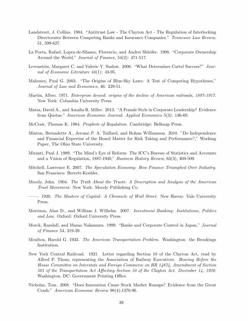
Landstreet, J. Collins. 1984. “Antitrust Law - The Clayton Act - The Regulation of InterlockingDirectorates Between Competing Banks and Insurance Companies.” Tennessee Law Review,51, 599-627.

La Porta, Rafael, Lopez-de-Silanez, Florencio, and Andrei Shleifer. 1998. “Corporate OwnershipAround the World,” Journal of Finance, 54(2): 471-517.

Levenstein, Margaret C. and Valerie Y. Suslow. 2006. “What Determines Cartel Success?” Jour-nal of Economic Literature 44(1): 43-95.

Mahoney, Paul G. 2003. “The Origins of Blue-Sky Laws: A Test of Competing Hypotheses,”Journal of Law and Economics, 46: 229-51.

Martin, Albro. 1971. Enterprise denied: origins of the decline of American railroads, 1897-1917.New York: Columbia University Press.

Matsa, David A., and Amalia R. Miller. 2013. “A Female Style in Corporate Leadership? Evidencefrom Quotas.” American Economic Journal: Applied Economics 5(3): 136-69.

McCraw, Thomas K. 1984. Prophets of Regulation. Cambridge: Belknap Press.

Minton, Bernadette A., Jerome P. A. Taillard, and Rohan Williamson. 2010. ”Do Independenceand Financial Expertise of the Board Matter for Risk Taking and Performance?,” WorkingPaper, The Ohio State University.

Miranti, Paul J. 1989. “The Mind’s Eye of Reform: The ICC’s Bureau of Statistics and Accountsand a Vision of Regulation, 1887-1940,” Business History Review, 63(3), 469-509.

Mitchell, Lawrence E. 2007. The Speculation Economy: How Finance Triumphed Over Industry.San Francisco: Berrett-Koehler.

Moody, John. 1904. The Truth About the Trusts: A Description and Analysis of the AmericanTrust Movement. New York: Moody Publishing Co.

——. 1920. The Masters of Capital: A Chronicle of Wall Street. New Haven: Yale UniversityPress.

Morrison, Alan D., and William J. Wilhelm. 2007. Investment Banking: Institutions, Politicsand Law. Oxford: Oxford University Press.

Morck, Randall, and Masao Nakamura. 1999. “Banks and Corporate Control in Japan,” Journalof Finance 54, 319-39.

Moulton, Harold G. 1933. The American Transportation Problem. Washington: the BrookingsInstitution.

New York Central Railroad. 1921. Letter regarding Section 10 of the Clayton Act, read byAlfred P. Thom, representing the Association of Railway Executives. Hearing Before theHouse Committee on Interstate and Foreign Commerce on HR 14674, Amendment of Section501 of the Transportation Act Affecting Section 10 of the Clayton Act. December 14, 1920.Washington, DC: Government Printing Office.

Nicholas, Tom. 2008. “Does Innovation Cause Stock Market Runups? Evidence from the GreatCrash.” American Economic Review 98(4):1370-96.

39

Nygaard, Knut. 2011. “Forced Board Changes: Evidence from Norway.” Working Paper, OsloSchool of Business.

Peach, William N. 1975. The Security Affiliates of National Banks. New York: Arno Press.

Philippon, Thomas, and Ariell Reshef. 2009. “Wages and Human Capital in the U.S. FinancialIndustry, 1909-2006.” Working paper, NYU.

Pujo Committee. [U.S. Congress, House Committee on Banking and Currency.] 1913a. MoneyTrust Investigation: Hearings Before the Committee Appointed Pursuant to House Resolu-tions 429 and 504 to Investigate the Concentration of Control of Money and Credit. Wash-ington DC: Government Printing Office.

——. 1913b. Report of the Committee Appointed Pursuant to House Resolutions 429 and 504 toInvestigate the Concentration of Control of Money and Credit. Washington DC: GovernmentPrinting Office.

Ramirez, Carlos D. 1995. “Did J.P. Morgan’s Men Add Liquidity? Corporate Investment, CashFlow, and Financial Structure at the Turn of the Twentieth Century,” Journal of Finance,50(2), 661-78.

Ramirez, Carlos D., and Christian Eigen-Zucchi. 2001. “Understanding the Clayton Act of 1914:An Analysis of the Interest Group Hypothesis,” Public Choice, 106(1-2), 157-81.

Ramirez, Carlos D., and J. Bradford DeLong. 1996. “Banker Influence and Business EconomicPerformance: Assessing the Impact of Depression-Era Financial Reforms,” in Bordo andSylla, eds., Anglo-American Financial Systems: Institutions and Markets in the TwentiethCentury. New York: Irwin.

—— and ——. 2001. “Understanding America’s Hesitant Steps Toward Financial Capitalism:Politics, the Depression, and the Separation of Commercial and Investment Banking,” PublicChoice, 106(1-2), 93-116.

Rajan, Rghuram G. 1992. “Insiders and Outsiders: The Choice between Informed and Arm’s-Length Debt.” Journal of Finance, 47(4): 1367-1400.

Redlich, Fritz. 1951. The Molding of American Banking: Men and Ideas. New York: HafnerPublishing Co.

Ripley, William Z. 1912. Railroads: Rates and Regulation. New York: Longmans, Green and Co.

——.1915. Railroads: Finance and Organization. New York: Longmans, Green and Co.

Rockoff, Hugh. 2000. “Banking and Finance, 1789-1914,” in Engerman and Gallman, eds. Cam-bridge Economic History of the United States. New York: Cambridge University Press.

Roe, Mark. 1993. “Some Differences in Corporate Structure in Germany, Japan, and the UnitedStates.” Yale Law Journal 102: 1927.

Roe, Mark. 1994. Strong Managers, Weak Owners: The Political Roots of American CorporateFinance. Princeton: Princeton University Press.

Sakolski, Aaron. 1913. American Railroad Economics: A Text-Book for Investors and Students.New York: MacMillan.

40

Sharpe, Steven A. 1990. “Asymmetric Information, Bank Lending, and Implicit Contracts: AStylized Model of Customer Relationships.” Journal of Finance 45(4):1069-87.

Seligman, Joel. 1982. The Transformation of Wall Street: A History of the Securities and Ex-change Commission and Modern Corporate Finance. Boston: Houghton Mifflin.

Sivakumar, Kumar N., and Gregory Waymire. 2003. “Enforceable Accounting Rules and IncomeMeasurement by Early 20th Century Railroads,” Journal of Accounting Research, 41(2), 397-432.

Smith, George D., and Richard Sylla. 1993. The Transformation of Financial Capitalism: AnEssay on The History of American Capital Markets. New York: Blackwell.

Stevenson, Betsey. 2010. “Beyond the Classroom: Using Title IX to Measure the Return to HighSchool Sports.” Review of Economics and Statistics 92: 284-301.

Stover, John F. 1961. American Railroads. Chicago: University of Chicago Press.

Strouse, Jean. 1999. Morgan: American Financier. Cambridge: Harvard University Press

Sylla, Richard. 1975. The American Capital Market, 1846-1914. New York: Arno Press.

Todd, Albert M. 1919. “Statement of Albert M. Todd, President of the Public Ownership Leagueof America,” in Hearings Before the Committee on Interstate Commerce, 65th Cong. 3rdSess., Vol. I. Washington, DC: Gov’t Printing Office.

Weinstein, David E., and Yishay Yafeh. 1998. “On the Costs of a Bank-Centered FinancialSystem: Evidence from the Changing Main Bank Relations in Japan,” Journal of Finance,53(2), 635-72.

White, Eugene. 1983. The Regulation and Reform of the American Banking System, 1900-1929.Princeton: Princeton University Press.

White, Eugene. 1986. “Before the Glass Steagall Act: An Analysis of the Investment BankingActivities of National Banks.” Explorations in Economic History, 23(1), 33-55.

White, Eugene. 1990. “The Stock Market Boom and Crash of 1929 Revisited.” Journal ofEconomic Perspectives 4(2):67-83.

White, Richard. 2012. Railroaded: The Transcontinentals and the Making of Modern America.New York: W.W. Norton.

William & Mary Law Review, Note. 1976. “The Penn Central Reorganization: A New Look atSection 10 of the Clayton Act,” William & Mary Law Review 17(4-5): 737-56.

Willis, Parker and John Bogen. 1929. Investment Banking. New York: Harper and Row.

Wilson, Woodrow. 1913. The New Freedom: A Call for the Emancipation of the GenerousEnergies of a People. New York: Doubleday.

Wilson, Woodrow. 1914. “An Address on Antitrust Legislation to a Joint Session of Congress,”20 January 1914, in Papers of Woodrow Wilson, vol. 29, p. 155. Princeton: PrincetonUniversity Press.

41

1905 1910 1915 1920 1925 19300

0.1

0.2

0.3

0.4

0.5

0.6

0.7

0.8

Clayton ActPassed

Section 10Implemented

Industrials

Railroads

Figure 1:Proportion of bond underwriting by banks represented on boards, 1907-29

Note: The figure presents a three-year moving average of the proportion of debt that was underwritten by investment banksrepresented on the boards of NYSE-listed railroads, and industrial companies listed on the NYSE in 1913. The figure iscalculated from all sample railroads’ and industrials’ debt issues, which totalled 638 different bond offerings for the railroads,and 141 for the industrials. For each issue, the amount underwritten by bankers on the firms’ boards is calculated as theproportion of the underwriters that were represented on the firm’s board multiplied by the value of the issue. For each year,the overall proportion of debt underwritten by bankers on boards is calculated as the sum of those amounts divided by thetotal amount of debt issues for the sample firms in that year. For additional information, see the Appendix.

42

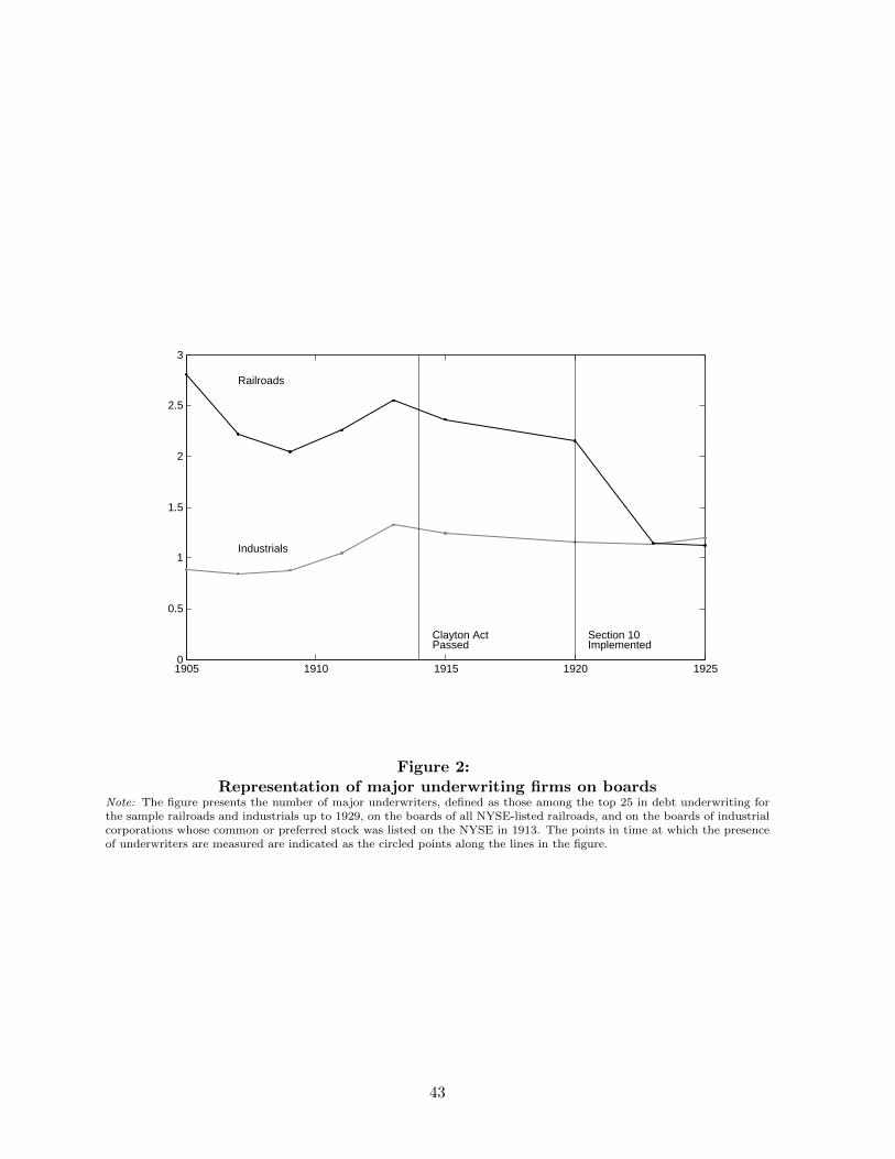
1905 1910 1915 1920 19250

0.5

1

1.5

2

2.5

3

Clayton ActPassed

Section 10Implemented

Railroads

Industrials

Figure 2:Representation of major underwriting firms on boards

Note: The figure presents the number of major underwriters, defined as those among the top 25 in debt underwriting forthe sample railroads and industrials up to 1929, on the boards of all NYSE-listed railroads, and on the boards of industrialcorporations whose common or preferred stock was listed on the NYSE in 1913. The points in time at which the presenceof underwriters are measured are indicated as the circled points along the lines in the figure.

43

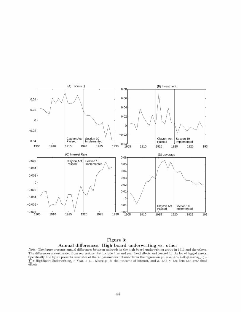
1905 1910 1915 1920 1925 1930

−0.04

−0.02

0

0.02

0.04

(A) Tobin’s Q

Clayton ActPassed

Section 10Implemented

1905 1910 1915 1920 1925 1930−0.04

−0.02

0

0.02

0.04

0.06

0.08(B) Investment

Clayton ActPassed

Section 10Implemented

1905 1910 1915 1920 1925 1930−0.008

−0.006

−0.004

−0.002

0

0.002

0.004

0.006

(C) Interest Rate

Clayton ActPassed

Section 10Implemented

1905 1910 1915 1920 1925 1930−0.02

−0.01

0

0.01

0.02

0.03

0.04

0.05

0.06(D) Leverage

Clayton ActPassed

Section 10Implemented

Figure 3:Annual differences: High board underwriting vs. other

Note: The figure presents annual differences between railroads in the high board underwriting group in 1913 and the others.The differences are estimated from regressions that include firm and year fixed effects and control for the log of lagged assets.Specifically, the figure presents estimates of the πt parameters obtained from the regression yit = αi +γt +δlog(assetst−1)+∑πtHighBoardUnderwritingi × Yeart + εit, where yit is the outcome of interest, and αi and γt are firm and year fixed

effects.

44

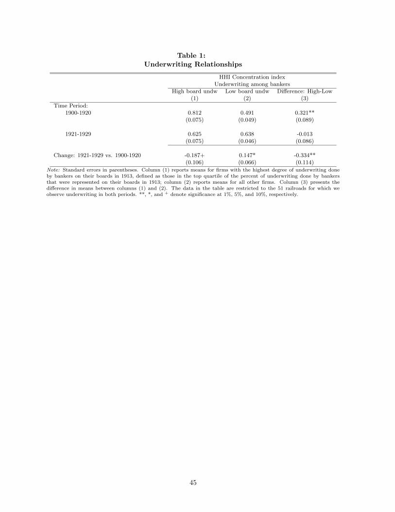
Table 1:Underwriting Relationships

HHI Concentration indexUnderwriting among bankers

High board undw Low board undw Difference: High-Low(1) (2) (3)

Time Period:1900-1920 0.812 0.491 0.321**

(0.075) (0.049) (0.089)

1921-1929 0.625 0.638 -0.013(0.075) (0.046) (0.086)

Change: 1921-1929 vs. 1900-1920 -0.187+ 0.147* -0.334**(0.106) (0.066) (0.114)

Note: Standard errors in parentheses. Column (1) reports means for firms with the highest degree of underwriting doneby bankers on their boards in 1913, defined as those in the top quartile of the percent of underwriting done by bankersthat were represented on their boards in 1913; column (2) reports means for all other firms. Column (3) presents thedifference in means between columns (1) and (2). The data in the table are restricted to the 51 railroads for which weobserve underwriting in both periods. **, *, and + denote significance at 1%, 5%, and 10%, respectively.

45

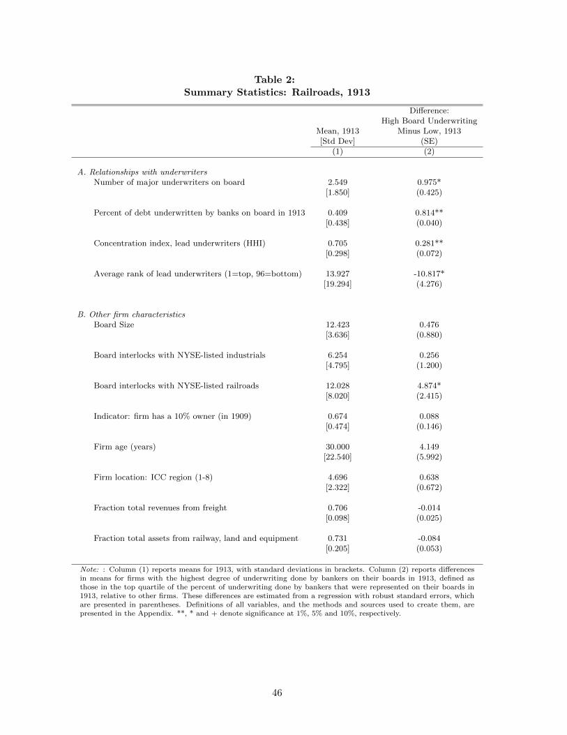
Table 2:Summary Statistics: Railroads, 1913

Difference:High Board Underwriting

Mean, 1913 Minus Low, 1913[Std Dev] (SE)

(1) (2)

A. Relationships with underwritersNumber of major underwriters on board 2.549 0.975*

[1.850] (0.425)

Percent of debt underwritten by banks on board in 1913 0.409 0.814**[0.438] (0.040)

Concentration index, lead underwriters (HHI) 0.705 0.281**[0.298] (0.072)

Average rank of lead underwriters (1=top, 96=bottom) 13.927 -10.817*[19.294] (4.276)

B. Other firm characteristicsBoard Size 12.423 0.476

[3.636] (0.880)

Board interlocks with NYSE-listed industrials 6.254 0.256[4.795] (1.200)

Board interlocks with NYSE-listed railroads 12.028 4.874*[8.020] (2.415)

Indicator: firm has a 10% owner (in 1909) 0.674 0.088[0.474] (0.146)

Firm age (years) 30.000 4.149[22.540] (5.992)

Firm location: ICC region (1-8) 4.696 0.638[2.322] (0.672)

Fraction total revenues from freight 0.706 -0.014[0.098] (0.025)

Fraction total assets from railway, land and equipment 0.731 -0.084[0.205] (0.053)

Note: : Column (1) reports means for 1913, with standard deviations in brackets. Column (2) reports differencesin means for firms with the highest degree of underwriting done by bankers on their boards in 1913, defined asthose in the top quartile of the percent of underwriting done by bankers that were represented on their boards in1913, relative to other firms. These differences are estimated from a regression with robust standard errors, whichare presented in parentheses. Definitions of all variables, and the methods and sources used to create them, arepresented in the Appendix. **, * and + denote significance at 1%, 5% and 10%, respectively.

46

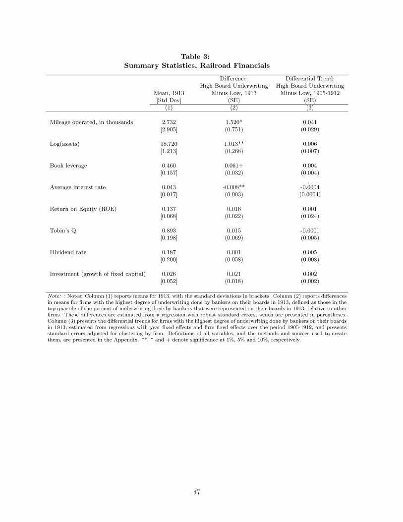
Table 3:Summary Statistics, Railroad Financials

Difference: Differential Trend:High Board Underwriting High Board Underwriting

Mean, 1913 Minus Low, 1913 Minus Low, 1905-1912[Std Dev] (SE) (SE)

(1) (2) (3)

Mileage operated, in thousands 2.732 1.520* 0.041[2.905] (0.751) (0.029)

Log(assets) 18.720 1.013** 0.006[1.213] (0.268) (0.007)

Book leverage 0.460 0.061+ 0.004[0.157] (0.032) (0.004)

Average interest rate 0.043 -0.008** -0.0004[0.017] (0.003) (0.0004)

Return on Equity (ROE) 0.137 0.016 0.001[0.068] (0.022) (0.024)

Tobin’s Q 0.893 0.015 -0.0001[0.198] (0.069) (0.005)

Dividend rate 0.187 0.001 0.005[0.200] (0.058) (0.008)

Investment (growth of fixed capital) 0.026 0.021 0.002[0.052] (0.018) (0.002)

Note: : Notes: Column (1) reports means for 1913, with the standard deviations in brackets. Column (2) reports differencesin means for firms with the highest degree of underwriting done by bankers on their boards in 1913, defined as those in thetop quartile of the percent of underwriting done by bankers that were represented on their boards in 1913, relative to otherfirms. These differences are estimated from a regression with robust standard errors, which are presented in parentheses.Column (3) presents the differential trends for firms with the highest degree of underwriting done by bankers on their boardsin 1913, estimated from regressions with year fixed effects and firm fixed effects over the period 1905-1912, and presentsstandard errors adjusted for clustering by firm. Definitions of all variables, and the methods and sources used to createthem, are presented in the Appendix. **, * and + denote significance at 1%, 5% and 10%, respectively.

47

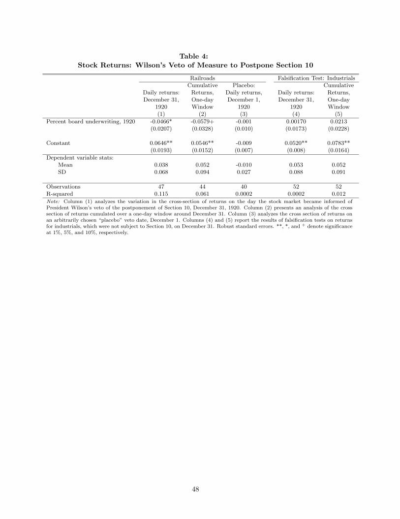
Table 4:Stock Returns: Wilson’s Veto of Measure to Postpone Section 10

Railroads Falsification Test: IndustrialsCumulative Placebo: Cumulative

Daily returns: Returns, Daily returns, Daily returns: Returns,December 31, One-day December 1, December 31, One-day

1920 Window 1920 1920 Window(1) (2) (3) (4) (5)

Percent board underwriting, 1920 -0.0466* -0.0579+ -0.001 0.00170 0.0213(0.0207) (0.0328) (0.010) (0.0173) (0.0228)

Constant 0.0646** 0.0546** -0.009 0.0520** 0.0783**(0.0193) (0.0152) (0.007) (0.008) (0.0164)

Dependent variable stats:Mean 0.038 0.052 -0.010 0.053 0.052SD 0.068 0.094 0.027 0.088 0.091

Observations 47 44 40 52 52R-squared 0.115 0.061 0.0002 0.0002 0.012

Note: Column (1) analyzes the variation in the cross-section of returns on the day the stock market became informed ofPresident Wilson’s veto of the postponement of Section 10, December 31, 1920. Column (2) presents an analysis of the crosssection of returns cumulated over a one-day window around December 31. Column (3) analyzes the cross section of returns onan arbitrarily chosen “placebo” veto date, December 1. Columns (4) and (5) report the results of falsification tests on returnsfor industrials, which were not subject to Section 10, on December 31. Robust standard errors. **, *, and + denote significanceat 1%, 5%, and 10%, respectively.

48

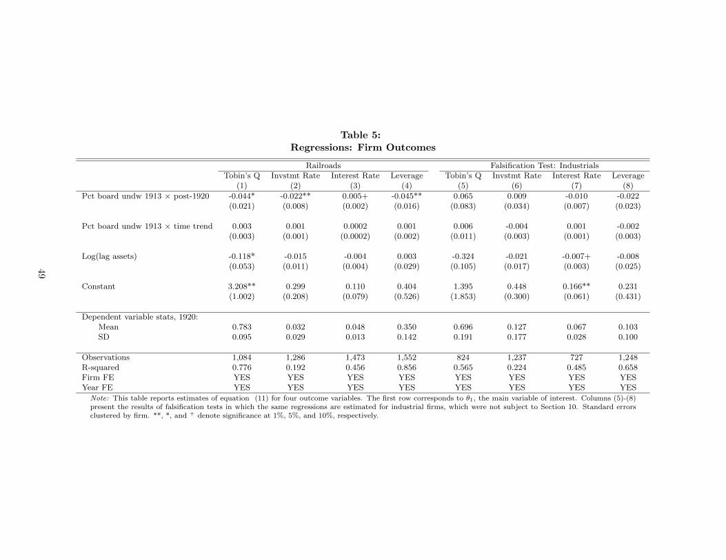
Table 5:Regressions: Firm Outcomes

Railroads Falsification Test: IndustrialsTobin’s Q Invstmt Rate Interest Rate Leverage Tobin’s Q Invstmt Rate Interest Rate Leverage

(1) (2) (3) (4) (5) (6) (7) (8)

Pct board undw 1913 × post-1920 -0.044* -0.022** 0.005+ -0.045** 0.065 0.009 -0.010 -0.022(0.021) (0.008) (0.002) (0.016) (0.083) (0.034) (0.007) (0.023)

Pct board undw 1913 × time trend 0.003 0.001 0.0002 0.001 0.006 -0.004 0.001 -0.002(0.003) (0.001) (0.0002) (0.002) (0.011) (0.003) (0.001) (0.003)

Log(lag assets) -0.118* -0.015 -0.004 0.003 -0.324 -0.021 -0.007+ -0.008(0.053) (0.011) (0.004) (0.029) (0.105) (0.017) (0.003) (0.025)

Constant 3.208** 0.299 0.110 0.404 1.395 0.448 0.166** 0.231(1.002) (0.208) (0.079) (0.526) (1.853) (0.300) (0.061) (0.431)

Dependent variable stats, 1920:Mean 0.783 0.032 0.048 0.350 0.696 0.127 0.067 0.103SD 0.095 0.029 0.013 0.142 0.191 0.177 0.028 0.100

Observations 1,084 1,286 1,473 1,552 824 1,237 727 1,248R-squared 0.776 0.192 0.456 0.856 0.565 0.224 0.485 0.658Firm FE YES YES YES YES YES YES YES YESYear FE YES YES YES YES YES YES YES YES

Note: This table reports estimates of equation (11) for four outcome variables. The first row corresponds to θ1, the main variable of interest. Columns (5)-(8)present the results of falsification tests in which the same regressions are estimated for industrial firms, which were not subject to Section 10. Standard errorsclustered by firm. **, *, and + denote significance at 1%, 5%, and 10%, respectively.

49

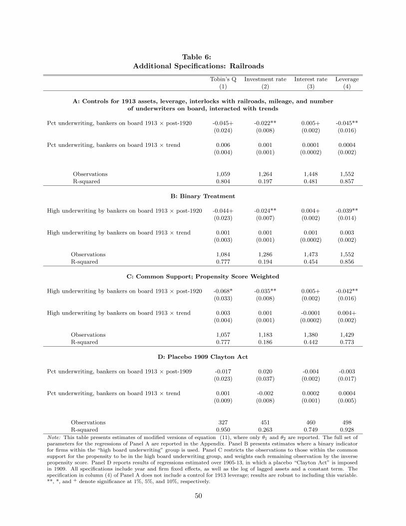
Table 6:Additional Specifications: Railroads

Tobin’s Q Investment rate Interest rate Leverage(1) (2) (3) (4)

A: Controls for 1913 assets, leverage, interlocks with railroads, mileage, and numberof underwriters on board, interacted with trends

Pct underwriting, bankers on board 1913 × post-1920 -0.045+ -0.022** 0.005+ -0.045**(0.024) (0.008) (0.002) (0.016)

Pct underwriting, bankers on board 1913 × trend 0.006 0.001 0.0001 0.0004(0.004) (0.001) (0.0002) (0.002)

Observations 1,059 1,264 1,448 1,552R-squared 0.804 0.197 0.481 0.857

B: Binary Treatment

High underwriting by bankers on board 1913 × post-1920 -0.044+ -0.024** 0.004+ -0.039**(0.023) (0.007) (0.002) (0.014)

High underwriting by bankers on board 1913 × trend 0.001 0.001 0.001 0.003(0.003) (0.001) (0.0002) (0.002)

Observations 1,084 1,286 1,473 1,552R-squared 0.777 0.194 0.454 0.856

C: Common Support; Propensity Score Weighted

High underwriting by bankers on board 1913 × post-1920 -0.068* -0.035** 0.005+ -0.042**(0.033) (0.008) (0.002) (0.016)

High underwriting by bankers on board 1913 × trend 0.003 0.001 -0.0001 0.004+(0.004) (0.001) (0.0002) (0.002)

Observations 1,057 1,183 1,380 1,429R-squared 0.777 0.186 0.442 0.773

D: Placebo 1909 Clayton Act

Pct underwriting, bankers on board 1913 × post-1909 -0.017 0.020 -0.004 -0.003(0.023) (0.037) (0.002) (0.017)

Pct underwriting, bankers on board 1913 × trend 0.001 -0.002 0.0002 0.0004(0.009) (0.008) (0.001) (0.005)

Observations 327 451 460 498R-squared 0.950 0.263 0.749 0.928

Note: This table presents estimates of modified versions of equation (11), where only θ1 and θ2 are reported. The full set ofparameters for the regressions of Panel A are reported in the Appendix. Panel B presents estimates where a binary indicatorfor firms within the “high board underwriting” group is used. Panel C restricts the observations to those within the commonsupport for the propensity to be in the high board underwriting group, and weights each remaining observation by the inversepropensity score. Panel D reports results of regressions estimated over 1905-13, in which a placebo “Clayton Act” is imposedin 1909. All specifications include year and firm fixed effects, as well as the log of lagged assets and a constant term. Thespecification in column (4) of Panel A does not include a control for 1913 leverage; results are robust to including this variable.**, *, and + denote significance at 1%, 5%, and 10%, respectively.

50

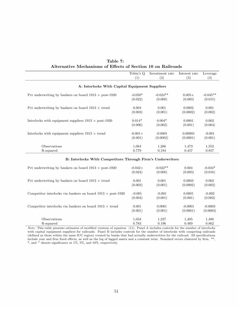
Table 7:Alternative Mechanisms of Effects of Section 10 on Railroads

Tobin’s Q Investment rate Interest rate Leverage(1) (2) (3) (4)

A: Interlocks With Capital Equipment Suppliers

Pct underwriting by bankers on board 1913 × post-1920 -0.050* -0.024** 0.005+ -0.045**(0.022) (0.008) (0.003) (0.015)

Pct underwriting by bankers on board 1913 × trend 0.004 0.001 0.0002 0.001(0.003) (0.001) (0.0002) (0.002)

Interlocks with equipment suppliers 1913 × post-1920 0.014* 0.004* 0.0001 0.002(0.006) (0.002) (0.001) (0.004)

Interlocks with equipment suppliers 1913 × trend -0.001+ -0.0001 0.00003 -0.001(0.001) (0.0002) (0.0001) (0.001)

Observations 1,084 1,286 1,473 1,552R-squared 0.779 0.194 0.457 0.857

B: Interlocks With Competitors Through Firm’s Underwriters

Pct underwriting by bankers on board 1913 × post-1920 -0.042+ -0.022** 0.004 -0.034*(0.024) (0.008) (0.003) (0.016)

Pct underwriting by bankers on board 1913 × trend 0.001 0.001 0.0003 0.002(0.003) (0.001) (0.0002) (0.002)

Competitor interlocks via bankers on board 1913 × post-1920 -0.001 -0.001 0.0001 -0.002(0.004) (0.001) (0.001) (0.002)

Competitor interlocks via bankers on board 1913 × trend 0.001 0.0001 -0.0001 -0.0003(0.001) (0.001) (0.0001) (0.0003)

Observations 1,034 1,227 1,405 1,488R-squared 0.783 0.196 0.469 0.862

Note: This table presents estimates of modified versions of equation (11). Panel A includes controls for the number of interlockswith capital equipment suppliers for railroads. Panel B includes controls for the number of interlocks with competing railroads(defined as those within the same ICC region) created by banks that had actually underwritten for the railroad. All specificationsinclude year and firm fixed effects, as well as the log of lagged assets and a constant term. Standard errors clustered by firm. **,*, and + denote significance at 1%, 5%, and 10%, respectively.

51

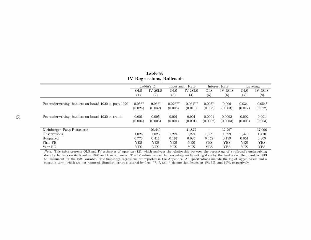
Table 8:IV Regressions, Railroads

Tobin’s Q Investment Rate Interest Rate LeverageOLS IV-2SLS OLS IV-2SLS OLS IV-2SLS OLS IV-2SLS(1) (2) (3) (4) (5) (6) (7) (8)

Pct underwriting, bankers on board 1920 × post-1920 -0.056* -0.066* -0.026** -0.031** 0.005* 0.006 -0.034+ -0.054*(0.025) (0.032) (0.008) (0.010) (0.003) (0.003) (0.017) (0.022)

Pct underwriting, bankers on board 1920 × trend 0.001 0.005 0.001 0.001 0.0001 0.0002 0.002 0.001(0.004) (0.005) (0.001) (0.001) (0.0002) (0.0003) (0.003) (0.003)

Kleinbergen-Paap F-statistic – 20.440 – 41.872 – 32.297 – 37.096Observations 1,025 1,025 1,224 1,224 1,399 1,399 1,470 1,470R-squared 0.773 0.411 0.197 0.084 0.452 0.199 0.851 0.309Firm FE YES YES YES YES YES YES YES YESYear FE YES YES YES YES YES YES YES YES

Note: This table presents OLS and IV estimates of equation (12), which analyzes the relationship between the percentage of a railroad’s underwritingdone by bankers on its board in 1920 and firm outcomes. The IV estimates use the percentage underwriting done by the bankers on the board in 1913to instrument for the 1920 variable. The first-stage regressions are reported in the Appendix. All specifications include the log of lagged assets and aconstant term, which are not reported. Standard errors clustered by firm. **, *, and + denote significance at 1%, 5%, and 10%, respectively.

52

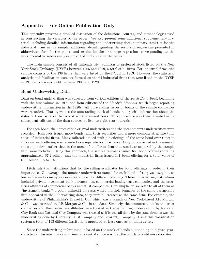
Appendix - For Online Publication Only

This appendix presents a detailed discussion of the definitions, sources, and methodologies usedin constructing the variables of the paper. We also present some additional supplementary ma-terial, including detailed information regarding the underwriting data, summary statistics for theindustrial firms in the sample, additional detail regarding the results of regressions presented inabbreviated form in the paper, and results for the first-stage regressions corresponding to theinstrumental variables analysis presented in Table 8 in the paper.

The main sample consists of all railroads with common or preferred stock listed on the NewYork Stock Exchange (NYSE) between 1905 and 1929, a total of 71 firms. For industrial firms, thesample consists of the 138 firms that were listed on the NYSE in 1913. However, the statisticalanalysis and falsification tests are focused on the 64 industrial firms that were listed on the NYSEin 1913 which issued debt between 1905 and 1929.

Bond Underwriting Data

Data on bond underwriting was collected from various editions of the Fitch Bond Book, beginningwith the first volume in 1913, and from editions of the Moody’s Manuals, which began reportingunderwriting information in the 1920s. All outstanding issues of bonds of the sample companieswere recorded. That is, we use the outstanding stock of bonds, along with information about thedates of their issuance, to reconstruct the annual flows. This procedure was then repeated usingsubsequent editions of the data sources at five- to eight-year intervals.

For each bond, the names of the original underwriters and the total amounts underwritten wererecorded. Railroads issued more bonds, and their securities had a more complex structure thanthose of industrial firms. Many railroads issued multiple offerings of the same bond over time; inthis case, each offering was recorded as a separate bond issuance. Only bonds issued in the name ofthe sample firm, rather than in the name of a different firm that was later acquired by the samplefirm, were included. Using this approach, the sample railroads issued 638 bond offerings totalingapproximately $7.2 billion, and the industrial firms issued 141 bond offering for a total value of$1.5 billion, up to 1929.

Fitch lists the institutions that led the selling syndicates for bond offerings in order of theirimportance. On average, the number underwriters named for each bond offering was two, but asfew as one and as many as eleven were listed for different offerings. These underwriting institutionsincluded private investment bank partnerships, commercial banks, trust companies, and the secu-rities affiliates of commercial banks and trust companies. (For simplicity, we refer to all of them as“investment banks,” broadly defined.) In cases where multiple branches of the same partnershipfirm appeared in the underwriting data, they were all treated as the same firm. For example, theunderwriting of Philadelphia’s Drexel & Co., which was a branch of New York-based J.P. Morgan& Co., was ascribed to J.P. Morgan & Co. in the data. Similarly, the commercial banks and trustcompanies and their securities affiliates were treated as the same firm; underwriting by NationalCity Bank and National City Company was treated as if it was all done by the same firm, as was theunderwriting done by Guaranty Trust Company and Guaranty Company. Using this classificationsystem a total of 193 different institutions appeared at least once as an underwriter.

Since the underwriting information is based on the stock of bonds outstanding in a given year,collected at discrete intervals of time, a potential concern is that the our data could miss short-term

53

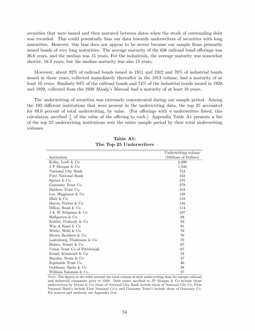
securities that were issued and then matured between dates when the stock of outstanding debtwas recorded. This could potentially bias our data towards underwriters of securities with longmaturities. However, this bias does not appear to be severe because our sample firms primarilyissued bonds of very long maturities. The average maturity of the 638 railroad bond offerings was26.6 years, and the median was 15 years. For the industrials, the average maturity was somewhatshorter, 16.3 years, but the median maturity was also 15 years.

Moreover, about 92% of railroad bonds issued in 1911 and 1912 and 70% of industrial bondsissued in those years, collected immediately thereafter in the 1913 volume, had a maturity of atleast 10 years. Similarly 94% of the railroad bonds and 74% of the industrial bonds issued in 1928and 1929, collected from the 1930 Moody’s Manual, had a maturity of at least 10 years.

The underwriting of securities was extremely concentrated during our sample period. Amongthe 193 different institutions that were present in the underwriting data, the top 25 accountedfor 89.6 percent of total underwriting, by value. (For offerings with n underwriters listed, thiscalculation ascribed 1

n of the value of the offering to each.) Appendix Table A1 presents a listof the top 25 underwriting institutions over the entire sample period by their total underwritingvolumes.

Table A1:The Top 25 Underwriters

Underwriting volumeInstitution (Millions of Dollars)

Kuhn, Loeb & Co 2,490J P Morgan & Co 1,540National City Bank 724First National Bank 542Speyer & Co 475Guaranty Trust Co 379Bankers Trust Co 163Lee, Higginson & Co 149Blair & Co 119Harris, Forbes & Co 116Dillon, Read & Co 114J & W Seligman & Co 107Hallgarten & Co 98Kidder, Peabody & Co 93Wm A Read & Co 91White, Weld & Co 79Brown Brothers & Co 76Ladenburg, Thalmann & Co 70Halsey, Stuart & Co 67Union Trust Co of Pittsburgh 67Kissel, Kinnicutt & Co 58Hayden, Stone & Co 47Equitable Trust Co 46Goldman, Sachs & Co 38William Salomon & Co 37

Note: The figures in the table present the total volume of debt underwriting done for sample railroadand industrial companies prior to 1929. Debt issues ascribed to JP Morgan & Co include thoseunderwritten by Drexel & Co; those of National City Bank include those of National City Co; FirstNational Bank’s include First National Co’s; and Guaranty Trust’s include those of Guaranty Co.For sources and methods, see Appendix text.

54

For the analysis of firms’ relationships with their underwriters, and of the frequency with whichthey use particular underwriters, we sometimes focus on the lead underwriter for each offering. Thelead underwriter is defined as the institution listed first by Fitch or Moody’s. The constructionof the data on underwriting by financial institutions represented on the boards of railroads andindustrial firms, and the construction of variables measuring the extent of such underwriting, arediscussed below.

Accounting Data

All accounting data were collected from various editions of the Moody’s Manuals of Railroads andCorporation Securities and the Moody’s Manuals of Investments of Industrial Securities. Thefinancial statements from which the data were recorded are quite varied in their content and levelof detail. In order to eliminate the potential for outliers to exert a significant influence on theestimation, all variables are trimmed at the top and bottom one percent.

The definitions of the variables utilized in the empirical analysis, along with some discussion ofhow the underlying data was coded, are presented below:

Book Leverage: Long-term debt/total assets. Long-term debt included bonds and ‘equipmenttrusts,’ which were bonds collateralized by railroads’ rolling stock, as well as other long-terminterest-bearing obligations such as mortgages.

Average Interest Rate: Total interest expense/interest-bearing liabilities. Interest-bearing liabil-ities include bonds, equipment trusts, mortgages and any other long-term interest-bearingobligations, as well as notes payable. For a handful of sample years, railroads consistentlyreported the total amount of ‘fixed charges,’ rather than interest expense on their incomestatements, which may have included items such as lease payments as well as interest. Ahandful of industrials also reported interest expenses in this way. Interest expense is availablefor fewer firm-years for the industrials than for the railroads, because a substantial numberof industrials had no long-term debt for many years of the sample. In addition, this variablewas sometimes not disclosed by industrials that had outstanding debt, or if it was disclosed,it was sometimes lumped together with other expense items.

Return on Equity (ROE): Earnings before interest and taxes/common shareholders’ equity. Earn-ings before interest and taxes is defined as operating revenues minus operating expenses.Common shareholders’ equity includes the book value of the common shares as well as thefirm’s ’surplus (retained earnings).

Dividend Payout Rate: Dividends paid on common stock/earnings before interest and taxes. Insome cases only total dividends (common plus preferred) were reported and the amount ofcommon dividends had to be calculated based on separate disclosures of the dividend rateand of the number of shares outstanding and the par value of the shares.

Investment rate: Change in the property and equipment account/previous year’s value of theproperty and equipment account. Accounting statements from the sample period generallydid not disclose capital expenditures. We infer investment as the change in the propertyaccount. Railroads treated improvements in their track and equipment as cash expensesand did not account for depreciation. We therefore do not account for depreciation in ourcalculation of the change in their property account. In contrast, industrial firms depreciatedtheir property and equipment; when information on depreciation is available, we add it to

55

the change in property account to estimate capital expenditures. The investment variable isnot utilized for years when individual firms radically changed their accounting statements, forexample by adding their subsidiaries’ property to their own; underwent a major restructuring;or when a significant merger occurred.

Tobin’s Q : (Book value of total assets + market value of equity - book value of equity)/book valueof total assets. The market value of equity is calculated as the number of common sharesoutstanding multiplied by the price as of the last day of the year, as reported in the NewYork Times for railroads, and in the Global Financial Data, for industrials. The book valueof equity is calculated as the book value of common and any preferred shares, plus the firms’surplus (retained earnings).

As the discussion above makes clear, there was occasionally some variation in the way thesample firms reported the accounting information that was used to construct the above variables.As we entered and coded these data, we carefully noted problems and inconsistencies in each firms’financial statements, and we used this information to construct indicator variables that we setequal to one when a variable is mismeasured. In our panel regressions using the accounting data,we include these indicators as controls. These do not substantially affect the results, but they doimprove the precision of the estimates. The indicators that are included in the regressions areas follows: in the regressions for Tobin’s Q, we include an indicator that is equal to one when acomponent of Q, the company’s ‘surplus’ (retained earnings), is mismeasured; in the regressions forthe interest rate, we include an indicator for cases where interest is disclosed together with otherexpenses, usually as ‘fixed charges’; and in the regressions for leverage, we include an indicator forcases where a firm reports debts of an ambiguous character.

Other Railroad Characteristics

For the sample railroads, a number of other firm characteristics were obtained from a variety ofsources, as follows:

Board Size: The total number of directors, as reported in Moody’s.

Firm Has 10 Percent Owner : The presence of an owner (generally another railroad) holding morethan ten percent of the firm’s outstanding shares. The variable reflects data collected by theInterstate Commerce Commission (ICC), and reported in the New York Times on 16 January,1909.

Firm Age: The current year minus the year of the oldest date of incorporation reported in Moody’s.

Firm Location: Region to which the ICC assigned the railroad. We use the more detailed regionalclassification adopted by the ICC in the 1920s, as reported in Annual Report on the Statisticsof Railways in the United States for the Year Ended December 31, 1929. These regions were:New England, Great Lakes, Central Eastern, Pocahontas, Southern, Northwestern, CentralWestern, and Southwestern. We assign numbers to each region, with 1 for New England and9 for Southwestern.

Fraction Total Revenues From Freight : Freight revenue/total revenue, as reported in Moody’s.

Fraction Total Assets From Railway, Land and Equipment : Property account/total assets, asreported in Moody’s. The property account is frequently named “Road and Equipment” byrailroads.

56

Mileage: Total miles operated, as reported in Moody’s.

Board Data, Director Names & Matching Procedure

We obtain the names of officers and directors of sample railroads and industrial firms from Moody’s,at two- to five-year intervals from 1905 to 1925. Of the 193 investment banks (broadly defined)in the underwriting data, a small handful were based outside the United States, or did not enterthe data until after 1925. Eliminating those firms leaves 188 underwriters. In order to determinewhether a director or partner of those investment banks held a board seat with a sample railroad,the names of all partners and directors of the financial institutions engaged in underwriting werecollected. For the commercial banks and trust companies, the director names were obtained fromthe Rand McNally Bankers’ Directory. Most investment banking partnerships were members of theNYSE; we obtain the names of their partners from the NYSE Directory. For institutions that werenot members of the NYSE and not commercial banks or trust companies, a number of differentsources were consulted to obtain the names of the directors or partners, such as the directorySecurities Dealers of North America; the Directory of Directors of the city in which the firm wasbased; the Baltimore Blue Book ; newspapers such as the New York Times and the Commercialand Financial Chronicle; and other publications such as U.S. Investor and Moody’s.

We match the names of individuals across these samples to identify board interlocks betweenrailroads and bond underwriters, between industrials and bond underwriters, between industrialsand railroads, and between different railroads. We follow a thorough procedure to clean the collectednames and ensure the accuracy of the matches. First, we verify that matching is not hamperedby transcription errors or inconsistencies in the source material. Since the management of bothfinancial and nonfinancial firms was relatively stable over time, data obtained for the same firm fordifferent years was compared. For the names of individuals that do not match perfectly across years,we use an algorithm to find approximate matches in names in surrounding years. This procedureidentifies cases in which only one letter of the entire name differs across years. In this manner, weare able to identify transcription errors and inconsistencies in the source materials.

Most inconsistencies in the source materials result from alternative spellings of names that wouldhinder our ability to correctly identify the same individual across firms or years. Many of theseinconsistencies are resolved by a set of rules that we developed to standardize names. We use theserules only to address issues of capitalization, spacing, hyphens, and apostrophes. As an example,“DuPont” was chosen to represent the following variations, all of which appeared in source materials:“du Pont,” “Dupont,” “duPont,” and “Du Pont.” For the remaining inconsistencies, alternativesources such as biographies, newspapers, and various historical books are used to determine whethertwo names represent the same person. When we find that two names refer to the same individual,we resolve the inconsistency by ascribing the version used more frequently to the individual.

For the purpose of determining interlocks between different groups of firms (railroads, under-writers, and industrials), we would ideally use each director’s full name. However, Moody’s oftenreports only initials for first and middle names. Thus, we are constrained to match on names usingonly first initial, middle initial, last name, and suffix. This data restriction could lead to overesti-mating interlocks across boards whenever two individuals who share a last name have different firstand middle names with the same initials. To address this potential source of overmatching, we usedata on names across firms, institutions, and years to identify cases where two or more individualsshare the same first initial, middle initial, last name, and suffix, but where there is variation intheir full names for at least one of all their observations. We then use information from alternative

57

sources to provide first and middle names for these cases. Using this information we develop a newfull name variable, fullname d, which separately identifies individuals that would otherwise collapseto one person if we were to use the uncorrected first and middle initials. For example, Walter HTaylor from Norfolk & Western, William H Taylor from Bowling Green Trust Company and W HTaylor from American Writing Paper would all be incorrectly identified as the same person usingonly first and middle name initials. The use of additional sources allows determining whether W HTaylor was Walter, William, or a third person altogether (he was William). As we discuss below,this corrected name variable consistently identifies individuals across samples and years. Interlocksbetween nonfinancial firms and securities underwriters, as well as across firms within each of thesesamples, are found by identifying exact matches in the variable fullname d, which consists of firstinitial, middle initial, surname, and suffix, but includes additional information for individuals thatshare first and middle initials, as described above.

Even after carefully cleaning the data, it is possible that our sample could suffer from somedegree of overmatching. Of course, there is no reason to think that the degree of overmatchingwould change over time, so this problem is unlikely to be responsible for the patterns described inthe paper. Nonetheless, two or more individuals may have shared the same full name, in whichcase we would falsely identify a board interlock across the firms where those different individualsheld board seats. In order to test the reliability of our matching procedure and assess the extentthat it leads to overmatching, we use an external source to provide a validity check.

As part of their investigation of the “money trust,” the Pujo Committee constructed a detaileddescription of board interlocks between the major financial institutions (regardless of whether theyunderwrote securities or not) and nonfinancial firms in 1913. The report contains the informationon a total of 179 bankers who held a total of 155 seats on railroad boards. We independently use ourdata and matching procedure to identify the interlocks between these same financial institutionsand railroads. Our own data produces nearly identical patterns of board interlocks. Only fourrailroad board seats held by bankers identified by the Pujo report were not identified in our data;in each case this was because these individuals were not listed as directors in the Moody’s Manualof 1913. That is, it was not due to a fault in the matching procedure, but rather to an inconsistencyin our underlying source. Moreover, only one banker-director identified in our sample was not listedin the Pujo report. We conclude from this that our matching procedure is highly accurate, and itis unlikely to generate significant biases in the patterns present in our data.

Interlock and Underwriting Figures and Data

Figure 1 in the paper presents the number of major underwriters—that is, those among the top 25according to total value underwritten up to 1929—that were represented on the boards of railroadsand industrials whose common or preferred stock was listed on the NYSE in 1913. These datawere generated by matching the names of the directors of railroads and industrials, in each yearindicated on the figure, to the names of the partners and directors of the 25 top underwriters, usingthe procedure described in the previous section. A total of 138 industrials, and 71 railroads, werelisted on the NYSE in 1913 and are therefore included in the figure. The figure simply plots theaverage number of those underwriting firms represented on the nonfinancial firms’ boards duringthe indicated years.

Figure 2 in the paper presents a three-year moving average of the percentage of total under-writing conducted by investment banks (broadly defined) currently represented on the boards ofrailroads and industrial firms. For each issue, the amount underwritten by bankers on the firms’

58

boards is calculated as the proportion of the underwriters that were represented on the firm’s boardmultiplied by the value of the issue. That is, if the issue had 3 underwriters with 2 represented onthe board, the amount underwritten by bankers on the board would be 2

3 times the value of theissue. For each year, the overall proportion of debt underwritten by bankers on boards is calculatedas the sum of those amounts divided by the total amount of debt issues for the sample firms inthat year. The figure plots a three year moving average of those annual proportions. Interlocksbetween nonfinancial firms and underwriters were determined using the matching procedure de-scribed above. As the data in the figure present a moving average, the line for railroads does notfall immediately to zero in the figure in 1921. However, the value in that year was in fact zero, andin subsequent years it was close to zero.

The underwriting data used in the tables and regressions are calculated slightly differently.These variables, along with the board interlock variables, are defined as follows:

Percent board underwriting in 1913 (abbreviated “Pct board undw 1913” in the tables) is ourmain treatment variable. It is calculated as the fraction of the total value of a firm’s bondofferings up to 1913 underwritten by bankers represented on its board in 1913. That is, unlikethe data in Figure 2, which shows the extent of underwriting done by bankers currently on thefirms’ boards, this variable captures the fraction of underwriting prior to 1913 done only bythe bankers represented on the firms’ boards at the end of that period. It therefore presentsa measure of the strength of the relationship between the underwriters currently representedon the firms’ boards (if any), and the firm, in 1913, the year before the Clayton Act wasdebated and implemented. For each issue, the amount underwritten by bankers that wereon the firms’ boards in 1913 is calculated as the proportion of the underwriters that wererepresented on the firm’s board in 1913, multiplied by the value of the issue. That is, ifthe issue had 2 underwriters with 1 represented on the board in 1913, the amount would be12 times the value of the issue. These amounts are then summed, and divided by the totalamount of underwriting by the firm up to 1913.

Percent board underwriting in 1920. This is used in Tables 4 and 8 is calculated in the same wayas the percent board underwriting in 1913, except it focuses on the bankers on the board in1920, and all debt issues up through 1920.

High board underwriting is an indicator variable used in Tables 1, 2, 3, and 6, and in Figure 3.It is equal to one for those firms in the top quartile of the “percent board underwriting in1913” variable. Given the distribution of the percent board underwriting in 1913 variablein our sample, this measure is equivalent to an indicator variable for those railroads withabove-median levels of underwriting by banks represented on their boards, conditional onhaving some nonzero amount of underwriting done by bankers on the railroads’ boards.

Herfindahl-Hirschman Concentration Index (HHI) is used in Tables 1 and 2. It is calculated fromthe shares of a railroad’s bond offerings in which each bank was the lead underwriter. Thatis, if bank b was the lead underwriter for nb of a railroad’s N bond offerings, and there wereB different banks that acted as lead underwriters, the HHI index for the railroad would be∑B

b=1(nbN )2. In Table 1 the index is calculated for all bonds issued prior to 1921, and then

again for all bonds issued from 1921-29. In Table 2 the data presented are for all bonds issuedprior to 1913.

Interlocks with equipment suppliers is used in Table 7, and is calculated for railroad i in 1913 asthe number of NYSE-listed industrial firms that were likely suppliers of capital equipment to

59

railroads that shared at least one director in common with railroad i in that year. We definefirms that manufactured steel, locomotives, railroads cars, and parts of railroad cars as likelycapital equipment suppliers. The interlocks were identified using our matching proceduredefined above.

Competitor interlocks via underwriters on board is used in Table 7. It is calculated for railroad i in1913 as the number of direct competitors—defined as the railroads that operated in the sameregion, as defined by the ICC—that shared at least one director in common with railroadi, where that director is also a partner or director of a bank that has underwritten debt forrailroad i up to 1913. The interlocks were identified using our matching procedure definedabove.

Number of major underwriters on board : Number of the top 25 underwriting firms representedon a firm’s board. The top 25 underwriters are determined by the total volume of debtunderwriting for the sample industrials and railroads, and are listed in Table A1 above. Thepresence of these top underwriters on the sample firms’ boards is identified using our matchingprocedure defined above.

Average rank of lead underwriters: Average rank of the lead underwriters for the firm, up to1913. Lead underwriters are the institutions listed first for each debt offering. A total of 69institutions were lead underwriters for railroads. (Many more institutions underwrote debtfor the railroads, but only 69 were ever listed as the lead underwriter for an offering). Therank of each underwriter is defined based on the total value underwritten up through 1929,ranging from 1 for the highest-ranked underwriter to 69 for the lowest-ranked underwriter.For each firm, the average rank is calculated as follows. If bank b of overall rank rb was thelead underwriter for bond offerings summing to vb in value for a railroad, and if the totalvalue of the railroad’s debt offerings were V , then the average rank of the railroad’s leadunderwriters would be

∑b(vbV )rb.

Board interlocks with NYSE-listed industrials: Number of industrial firms in the sample withwhich the railroad has at least one director in common. The interlocks were identified usingour matching procedure defined above.

Board interlocks with NYSE-listed railroads: Number of railroads in the sample with which therailroad has at least one director in common. The interlocks were identified using our matchingprocedure defined above.

Summary Statistics, Industrials

Summary statistics for the board data and financial data of railroads are presented in the maintext. Here we present and discuss similar data for the industrials.

Means and standard deviations for the 64 industrials firms that issued debt between 1900 and1929 (and are therefore included in the statistical tests in the paper), are presented in column(1) of Table A2 for the year 1913. These data illustrate several differences between railroads andindustrials. Relative to railroads, industrials in 1913 were smaller and younger. The mean value oflog assets for railroads was 18.7, compared to 18.0 for industrials, and the mean age for railroadswas 30 years, compared to 16 years for industrials. Industrials were far less levered, likely reflectinghigh salability of the railroad’s collateral: their mean book leverage ratio was 0.14, compared to0.46 for railroads. Industrials were slightly profitable on average—their ROE was 0.15, compared

60

to the railroads’ 0.14—and they paid a higher share of their earnings out as dividends (0.22 vs.0.19). Industrials also had fewer top underwriters represented on their boards (1.8 vs. 2.5), butthey relied on underwriters on their boards for about the same fraction of their underwriting (0.37vs. 0.41).

Column (2) of Table A2 presents tests of differences in means between industrials with andwithout a high reliance on banks represented on their boards in 1913 for their bond underwritingup to 1913. As with the railroads, these firms are defined as those among the top quartile in theshare of underwriting volume done by the bankers on their boards in 1913. Among the railroads,this ‘high board underwriting’ group was larger, more levered, and paid lower interest rates ontheir debt. Among industrials, selection into close relationships with underwriters appears to havebeen quite similar: the sign of the differences in size, leverage and interest rates are the same thanthose found for railroads. However, only the difference in firm size is statistically significant withthe industrials. But unlike the railroads, the high board underwriting group of industrials enjoyedhigher valuations, and invested at slightly lower rates.

61

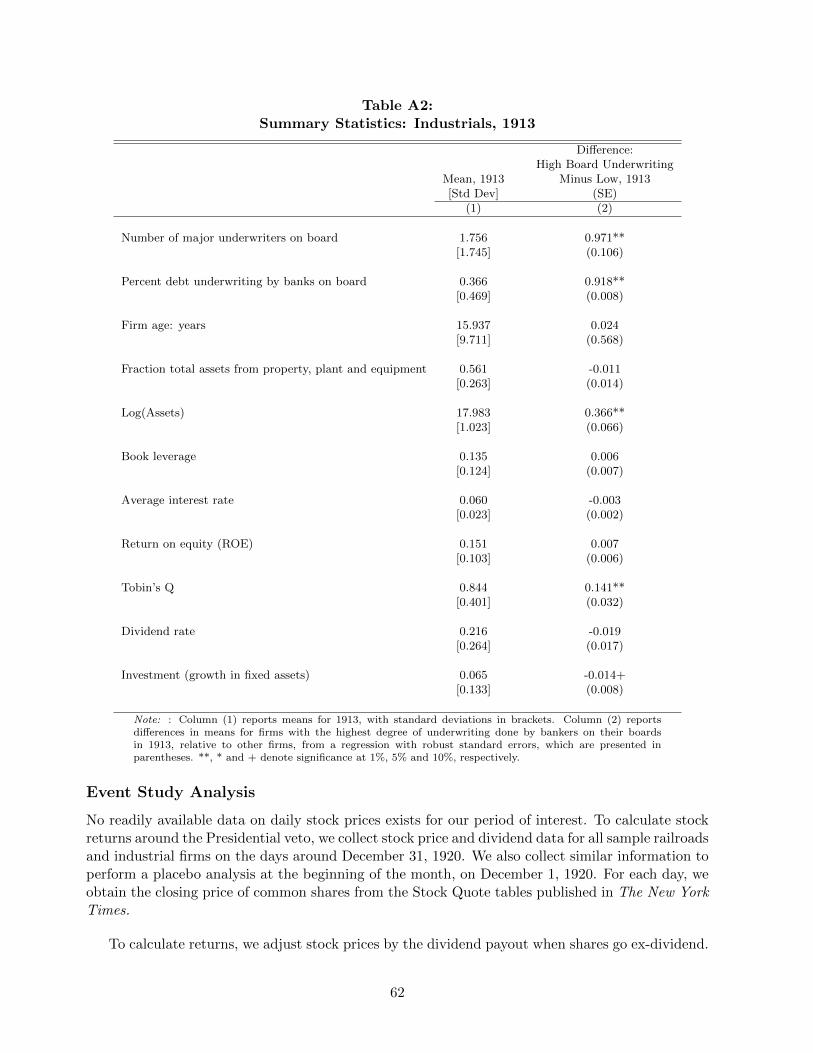
Table A2:Summary Statistics: Industrials, 1913

Difference:High Board Underwriting

Mean, 1913 Minus Low, 1913[Std Dev] (SE)

(1) (2)

Number of major underwriters on board 1.756 0.971**[1.745] (0.106)

Percent debt underwriting by banks on board 0.366 0.918**[0.469] (0.008)

Firm age: years 15.937 0.024[9.711] (0.568)

Fraction total assets from property, plant and equipment 0.561 -0.011[0.263] (0.014)

Log(Assets) 17.983 0.366**[1.023] (0.066)

Book leverage 0.135 0.006[0.124] (0.007)

Average interest rate 0.060 -0.003[0.023] (0.002)

Return on equity (ROE) 0.151 0.007[0.103] (0.006)

Tobin’s Q 0.844 0.141**[0.401] (0.032)

Dividend rate 0.216 -0.019[0.264] (0.017)

Investment (growth in fixed assets) 0.065 -0.014+[0.133] (0.008)

Note: : Column (1) reports means for 1913, with standard deviations in brackets. Column (2) reportsdifferences in means for firms with the highest degree of underwriting done by bankers on their boardsin 1913, relative to other firms, from a regression with robust standard errors, which are presented inparentheses. **, * and + denote significance at 1%, 5% and 10%, respectively.

Event Study Analysis

No readily available data on daily stock prices exists for our period of interest. To calculate stockreturns around the Presidential veto, we collect stock price and dividend data for all sample railroadsand industrial firms on the days around December 31, 1920. We also collect similar information toperform a placebo analysis at the beginning of the month, on December 1, 1920. For each day, weobtain the closing price of common shares from the Stock Quote tables published in The New YorkTimes.

To calculate returns, we adjust stock prices by the dividend payout when shares go ex-dividend.

62

We determine the ex-dividend date if the traded share was listed as such in the Stock Quotetable, and we obtain information on dividend payouts from the Moody’s Manual for the year 1921.Because the dividend payouts were mostly quoted as a percentage of the value of shares, we usethe par value of common shares, obtained from the same manual, to determine the dividend dollaramount when necessary. However, these adjustments make a negligible difference; the correlationbetween adjusted and unadjusted returns is above 0.98 for both dates in our analysis. There arealso no cases of stock splits within the days of our analysis.

On day t, we calculate firm’s i return as:

Ri,t =(Pi,t + di,t)− Pi,t−1

Pi,t−1(13)

Cumulative returns for a window of days [-k,k ] centered on December 31 or December 1, arecalculated as:

Cumulative Ri =t=k∑t=−k

Ri,t (14)

Our strategy diverges from the standard event study methodology because we cannot calculateabnormal returns as the difference between the actual return and the return predicted from amarket model. Estimating such a model would require collecting price and dividend data fromprimary sources for about a year prior to the veto, an exceedingly large data collection effort. Ourstrategy is therefore close to the market-adjusted-return model that assumes α = 0 and β = 1 forevery share.34 The lack of information on stock returns prior to the veto also limits our ability toadjust the standard errors using the pre-period variance in returns. Instead, we present placebotests based an earlier date, and on the returns of industrial firms.

Another limitation of historical stock market data is that securities markets were fairly illiquid.To be able to cumulate returns when some returns are missing within the event window, we assumeno price changes in days for which prices are missing, under the restriction that the number of non-missing returns observed during the event window [−k, k] for a firm were above the 25th percentileof non-missing returns in the sample. For railroads, this constraint requires observing at least twonon-missing returns in the three-day window around the veto. The constraint is not satisfied forthree railroads for which we observe returns on December 31, and accounts for the decline in thenumber of observations from column (1) to column (2) of Table 4.

Regression Results, Additional Detail

Panel A of Table 6 in the paper presents the estimates for the linear “percent underwriting bybankers on board in 1913” variable for the sample railroads of regressions that also include anumber of firm characteristics as controls. To conserve space, the parameter estimates associatedwith these firm characteristics are not reported in the table. Table A3 below present the full resultsof those regressions.

Table 8 in the paper reports the results of the second-stage of IV-2SLS regressions. For com-pleteness, the first-stage regressions corresponding to those results are reported in Tables A4 andA5 below.

34Because the event date is the same for all firms in the sample, subtracting the overall market return from thedaily individual stock return for all firms would only affect the constant term of the regression.

63

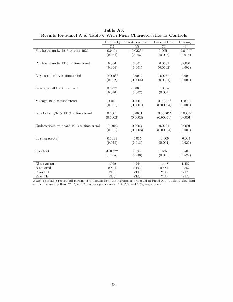
Table A3:Results for Panel A of Table 6 With Firm Characteristics as Controls

Tobin’s Q Investment Rate Interest Rate Leverage(1) (2) (3) (4)

Pct board undw 1913 × post-1920 -0.045+ -0.022** 0.005+ -0.045**(0.024) (0.008) (0.002) (0.016)

Pct board undw 1913 × time trend 0.006 0.001 0.0001 0.0004(0.004) (0.001) (0.0002) (0.002)

Log(assets)1913 × time trend -0.006** -0.0002 0.0003** 0.001(0.002) (0.0004) (0.0001) (0.001)

Leverage 1913 × time trend 0.023* -0.0003 0.001+(0.010) (0.002) (0.001)

Mileage 1913 × time trend 0.001+ 0.0001 -0.0001** -0.0001(0.001) (0.0001) (0.00004) (0.001)

Interlocks w/RRs 1913 × time trend 0.0001 -0.0001 -0.00003* -0.00004(0.0002) (0.0002) (0.00001) (0.0001)

Underwriters on board 1913 × time trend -0.0003 0.0003 0.0001 0.0001(0.001) (0.0006) (0.00004) (0.001)

Log(lag assets) -0.102+ -0.015 -0.005 -0.003(0.055) (0.013) (0.004) (0.029)

Constant 3.013** 0.294 0.135+ 0.500(1.025) (0.233) (0.068) (0.527)

Observations 1,059 1,264 1,448 1,552R-squared 0.804 0.197 0.481 0.857Firm FE YES YES YES YESYear FE YES YES YES YES

Note: This table reports all parameter estimates from the regressions presented in Panel A of Table 6. Standarderrors clustered by firm. **, *, and + denote significance at 1%, 5%, and 10%, respectively.

64

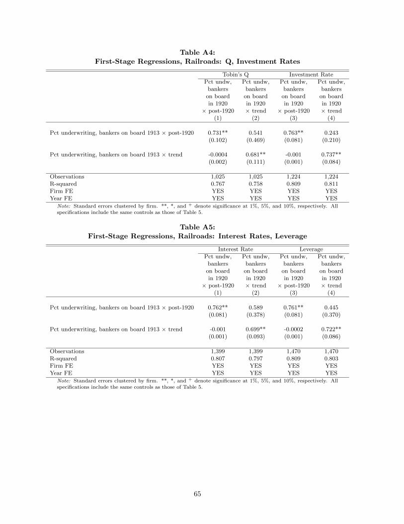
Table A4:First-Stage Regressions, Railroads: Q, Investment Rates

Tobin’s Q Investment RatePct undw, Pct undw, Pct undw, Pct undw,

bankers bankers bankers bankerson board on board on board on boardin 1920 in 1920 in 1920 in 1920

× post-1920 × trend × post-1920 × trend(1) (2) (3) (4)

Pct underwriting, bankers on board 1913 × post-1920 0.731** 0.541 0.763** 0.243(0.102) (0.469) (0.081) (0.210)

Pct underwriting, bankers on board 1913 × trend -0.0004 0.681** -0.001 0.737**(0.002) (0.111) (0.001) (0.084)

Observations 1,025 1,025 1,224 1,224R-squared 0.767 0.758 0.809 0.811Firm FE YES YES YES YESYear FE YES YES YES YES

Note: Standard errors clustered by firm. **, *, and + denote significance at 1%, 5%, and 10%, respectively. Allspecifications include the same controls as those of Table 5.

Table A5:First-Stage Regressions, Railroads: Interest Rates, Leverage

Interest Rate LeveragePct undw, Pct undw, Pct undw, Pct undw,

bankers bankers bankers bankerson board on board on board on boardin 1920 in 1920 in 1920 in 1920

× post-1920 × trend × post-1920 × trend(1) (2) (3) (4)

Pct underwriting, bankers on board 1913 × post-1920 0.762** 0.589 0.761** 0.445(0.081) (0.378) (0.081) (0.370)

Pct underwriting, bankers on board 1913 × trend -0.001 0.699** -0.0002 0.722**(0.001) (0.093) (0.001) (0.086)

Observations 1,399 1,399 1,470 1,470R-squared 0.807 0.797 0.809 0.803Firm FE YES YES YES YESYear FE YES YES YES YES

Note: Standard errors clustered by firm. **, *, and + denote significance at 1%, 5%, and 10%, respectively. Allspecifications include the same controls as those of Table 5.

65