Embed Size (px)
Citation preview
University of Mississippi University of Mississippi
eGrove eGrove
Electronic Theses and Dissertations Graduate School
2012
Investor Behavior Surrounding Trading Halts: Short Sales, Investor Behavior Surrounding Trading Halts: Short Sales,
Predation and Contagion Effects Predation and Contagion Effects
Mary Celeste Funck
Follow this and additional works at: https://egrove.olemiss.edu/etd
Part of the Finance Commons
Recommended Citation Recommended Citation Funck, Mary Celeste, "Investor Behavior Surrounding Trading Halts: Short Sales, Predation and Contagion Effects" (2012). Electronic Theses and Dissertations. 113. https://egrove.olemiss.edu/etd/113
This Dissertation is brought to you for free and open access by the Graduate School at eGrove. It has been accepted for inclusion in Electronic Theses and Dissertations by an authorized administrator of eGrove. For more information, please contact [email protected].
INVESTOR BEHAVIOR SURROUNDING TRADING HALTS:
SHORT SALES, PREDATION AND CONTAGION EFFECTS
DISSERTATION
A Dissertation
Presented in partial fulfillment of requirements
For the degree of Doctor of Philosophy
In the Department of Finance
The University of Mississippi
By
MARY C. FUNCK
August 2012

Copyright Mary C. Funck 2012
ALL RIGHTS RESERVED
ii
ABSTRACT
This dissertation is comprised of three essays that focus on the interaction between
exchange-mandated trading halts and short selling activity in the financial markets. In the first
essay, the behavior of short sellers is examined surrounding interruptions in trading to
determine if informed short sellers alter their trading patterns prior to and/or following a
trading halt. This investigation also addresses the impact of short sales on market quality for
halted stocks surrounding periods of interrupted trading, by examining returns, price volatility,
and spreads.
The second essay investigates if a short-selling contagion effect exists for contemporaries
of firms experiencing a trading halt. Although trading suspensions represent a firm-specific
event, they may be viewed as ‘contagious’ in the sense that they possess information relevant to
other firms in the same industry. The potential for an intra-industry effect supports an
examination into whether shorting levels vary significantly for organizations that are
informationally related to a firm experiencing a trading halt. The impact of short sales on the
market quality of these contemporary firms is also determined by examining returns, price
volatility, and spreads surrounding interruptions in trading for an industry member.
Market activity surrounding trading halts is examined in the third essay to determine if
predatory trading occurs. This research establishes if predatory behavior is present surrounding
interruptions in trading or alternatively, if trading halts eliminates the opportunity for predation.
This investigation also determines if documented changes in market quality for halted firms are
linked to predatory trading.

iii
LIST OF ABBREVIATIONS AND SYMBOLS
ADF National Association of Securities Dealers Alternative Display Facility
AMEX American Stock Exchange
ARCA Archipelago
CHX Chicago Stock Exchange
CRSP Center for Research in Security Prices
NASDAQ National Association of Securities Dealers
NYSE New York Stock Exchange
TAQ Trades and Quotes
WRDS Wharton Research Data Services

iv
TABLE OF CONTENTS
ABSTRACT ………………………………………………………………….……….…..… ii
LIST OF ABBREVIATIONS AND SYMBOLS …………………………………………….. iii
LIST OF TABLES ……………..…………………………………………………………… vi
LIST OF FIGURES …………………………………………………………………………… ix
ESSAY 1
INTRODUCTION ………………………………………………………………….. 2
HYPOTHESES (TRADING METRICS) …………………………..……………… 9
HYPOTHESES (MARKET QUALITY) …………………………………………….. 14
RESULTS …………………………………………………………………………… 25
CONCLUSION …………………………………………………………………….. 69
REFERENCES …………………………………………………………………….. 73
ESSAY 2
INTRODUCTION …………………………………………………………………. 79
HYPOTHESES ……………………………………………………………………. 87
RESULTS ………………………………………………………………………….. 102
CONCLUSION ……………………………………………………………………. 139
REFERENCES ……………………………………………………………………… 142
v
ESSAY 3
INTRODUCTION ………………………………………………………………….. 149
HYPOTHESES …………………………………………………………………….. 156
RESULTS …………………………………………………………………………… 163
CONCLUSION ……………………………………………………………………… 192
REFERENCES ……………………………………………………………………… 193
APPENDIX ………………………………………………………………………………… 197
VITA …………………………………………………………………………………….... 209
vi
LIST OF TABLES
ESSAY 1
1. Descriptive Statistics ……………………………………………………………….. 22
2. Average Daily Short Metrics ………………………………………………………. 27
3. Abnormal Short Selling Regression 1 ……………………………………………… 31
4. Abnormal Short Selling Regression 2 ……………………………………………… 34
5. Average Intraday Short Metrics …………………………………………………… 35
6. Post-halt Daily Returns …………………………………………………………….. 39
7. Daily Chi-Square Test ……………………………………………………………... 41
8. Intraday Post-halt Returns …………………………………………………………. 43
9. Intraday Chi-Square Test …………………………………………………………… 44
10. Weighted Price Contribution …………………………………………..………….. 49
11. Daily Mean Volatility Measures …………………………………………………… 51
12. Mean Interval Intraday Volatility Measures ………………………………………. 54
13. Mean Period Intraday Volatility Measures ………………………………………… 56
14. Spread Differences: 30-Minute Periods …………………………………………… 66
15. Spread Differences: 15-Second Periods …………………………………………… 67
ESSAY 2
1. Descriptive Statistics – Halts ………………………………………………………. 96
2. Descriptive Statistics – Halted Firms ……………………………………………….. 99
vii
3. Descriptive Statistics – Related Firms ……………………………………………... 100
4. Average Daily Short Metrics and Differences ……………………………………... 103
5. Abnormal Short Selling Regression 1 ………………………………………………. 108
6. Abnormal Short Selling Regression 2 ………………………………………………. 110
7. Intraday Short Metrics ……………………………………………………..……….. 112
8. Intraday Short Metric Differences …………………………………………………… 114
9. Post-halt Daily Returns ……………………………………………………………... 116
10. Daily Chi-Square Test ……………………………………………………………... 118
11. Intraday Post-halt Returns …………………………………………………………. 120
12. Intraday Chi-Square Test ………………………………………………………….. 121
13. Daily Mean Volatility Measures …………………………………………………… 124
14. Mean Interval Intraday Volatility Measures ……………………………………….. 126
15. Mean Period Intraday Volatility Measures ………………………………………… 129
16. Spread Differences: 30-Minute Periods …………………………………………… 134
17. Spread Differences: 15-Second Periods …………………………………………… 137
ESSAY 3
1. Descriptive Statistics ……………………………………………………………….. 161
2. Daily and Intraday Regressions …………………………………….……………… 166
3. Correlations and Granger Causality ………………………………………………... 168
4. Order Imbalance – Trading Volume ………………………………………………. 173
5. Order Imbalance – Number of Transactions ………………………………………… 174

viii
6. Abnormal Standardized Short Volume …………………………………………….. 180
7. Short Selling Order Imbalance …………………………………………………….. 182
8. Stocks with Large Price Declines …………………………………………………… 185

ix
LIST OF FIGURES
ESSAY 1
1. Daily Abnormal Short Selling ……………………………………………………. 28
2. Intraday Abnormal Short Selling ………………………………………………….. 36
3. Halt Day Trading and Short Selling Volume ………………………………………. 37
4. Speed of Price Adjustment ……………………………………………………….. 47
5. Intraday Volatility Measures ……………………………………………………… 58
6. Halt and Estimation Period Mean and Median Spreads …………………………… 60
7. Mean Intraday Spreads: 30-Minute Periods ………………………………………. 61
8. Mean Intraday Spreads: 1-Minute and 15-Second Periods ………………………. 62
9. Mean Intraday Spreads by Short Selling Levels …………………………………… 63
10. Differences in Spreads by Short Selling Levels …………………………………… 65
ESSAY 2
1. Daily Abnormal Short Selling ……………………………………………………. 104
2. Percent of Stocks with Daily Abnormal Short Selling Values …………………… 105
3. Halt and Estimation Period Median Spreads ……………………………………… 132
4. Intraday Spreads: 30-Minute Periods ……………………………………………… 133
5. Intraday Spreads: 1-Minute Periods ……………………………………………… 135
6. Intraday Spreads: 15-Second Periods ……………………………………………… 136

x
ESSAY 3
1. Abnormal Standardized Return ………………………………………………….. 165
2. Granger Causality …………………………………………………………………. 169
3. Volume and Number of Trades …………………………………………………… 171
4. Order Imbalance ………………………………………………………………….. 175
5. Short and Non-short Selling Volume and Percent of Trades …………………….. 178
6. Abnormal Standardized Short Volume ……………………………………………. 181
7. Short-selling Order Imbalance Differences ………………………………………. 183
8. Firms with Large Price Declines – by Period ……………………………………… 186
9. Cumulative Returns and Abnormal Short Selling …………………………………. 188
10. Cumulative Returns and Abnormal Short Selling: Reversal / No Reversal ………. 189
1
ESSAY 1:
DOES SHORT-SELLER INFORMATIVENESS EXTEND TO TRADING HALTS?
2
INTRODUCTION
We examine short selling activity surrounding trading halts to determine whether
informed short sellers alter their trading patterns prior to and/or following a trading halt by
changing the number, size, and/or total volume of short transactions they execute on halted
stocks. We also study the impact of short sales on market quality for halted stocks surrounding
periods of interrupted trading by examining their returns, price volatility and spreads.
Our investigation contributes to microstructure literature by addressing the impact of
short sales and trading halts together. We determine how these two trading mechanisms interact
and whether short sellers appreciably affect market quality and contribute to the impact on
security prices for firms experiencing a trading halt. Trading halts occur frequently in current
financial markets. Documenting the presence and the impact of short selling surrounding
interruptions in trading has important implications for individuals and institutions trading in the
markets and for those providing regulatory oversight.
TRADING INTERRUPTIONS
Major financial markets throughout the world have regulations that suspend trading under
specific, pre-specified circumstances. Kim and Yang (2004) categorize these trading
interruptions as either 1) price limits, which are triggered when security prices impede upon
boundaries established by market regulators, 2) firm-specific trading halts that are implemented
to stop trading on an individual security for a predetermined period or 3) market-wide circuit
3
breakers that halt trading on the entire market when a designated index breaches a pre-specified
level.
Firm specific trading halts can be further classified according to their underlying cause;
they can be either news-related or they can occur due to order imbalances. An order imbalance
trading halt is instigated when an exchange specialist observes a large imbalance between buy
and sell orders. A news-related trading halt is triggered by exchange officials when an
information release is expected to have or demonstrates a significant impact on security prices.
News-related trading halts, the focus of our investigation, are implemented to ensure that
new information is disseminated equally among market participants and to allow participants the
time necessary to gauge the impact of the news.1 Hauser, Kedar-Levy, Pilo, and Shurki (2006
page 83) state, “Trading halts are aimed at reducing information asymmetry by granting
investors the opportunity to reassess trades upon arrival of new, substantial information.”
The foundation of our investigation into the interaction between short-selling and news-
related trading halts relies on previous research findings. These include the informativeness of
short sales, the presence of asymmetric information surrounding the declaration of trading halts,
and the increase in trading activity by investors prior to interruptions in trading (the magnet
effect).
INFORMATIVENESS OF SHORT SELLERS
Research shows that short sellers are informed and it demonstrates that they have the
1 Trading halt discussion condensed from information contained on NASDAQ website at
http://www.nasdaq.com/about/marketwatch_faq.stm and SEC website at
http://www.sec.gov/answers/tradinghalt.htm
4
ability to earn abnormal returns in environments with elevated levels of information asymmetry.2
The foundation for this view rests upon the work of Miller (1977). He purports that in the
presence of short sale constraints, security prices tend to reflect a more optimistic valuation than
the average opinion of potential investors and thus prices tend to be biased upward. It follows
from Miller’s work that short sellers possess superior private information if their absence in the
market or their restricted ability to trade leads to overvalued security prices.
The rationale that short sellers are informed can also be justified by the heightened risk-
return profile of a short position (potentially unlimited losses) and the additional transaction
costs associated with shorting. For instance, Geczy, Musto, and Reed (2002 page 242) state, “…
short positions can be expensive or impossible and can be involuntarily terminated.” Dechow,
Hutton, Meulbroek, and Sloan (2001) purport that short sellers will trade only if they anticipate
that their superior knowledge will lead to gains that will compensate them for bearing elevated
risk and costs.
Short sellers are cross-sectionally more informed; this allows them to earn abnormal
returns by identifying and then short selling overpriced stocks and covering their position when
the prices on these securities drop. We suggest that the informational advantage of short sellers
extends to trading halts; our research intent is to determine whether short sellers use this
advantage to profit in the marketplace surrounding interruptions in trading.
Three empirical studies have particular significance for our investigation of short seller
behavior surrounding trading halts. In the first, Cohen, Diether, and Malloy (2007), examine the
relation between changes in the supply and demand for shorting and stock prices and find that
shorting demand is an important predictor of future stock returns. Particularly important for our
2 Senchack and Starks (1993); Arnold, Butler, Crack, and Zhang (2005); Chang, Cheng, and Yu (2007); Boehmer,
Jones, and Zhang (2008); and Diether, Lee, and Werner (2009B) provide specific examples.
5
examination of shorting in markets with high asymmetric information, their results are stronger
in trading environments with impeded public information flow.
In the second, Christophe, Ferri, and Angel (2004), investigate short-selling activity prior
to earnings announcements to determine if it differs from short selling during periods without an
imminent announcement. They find evidence of short seller informativeness through a
significant negative relation between pre-announcement short selling and post-announcement
stock prices. Additionally, they find that short selling does not increase across all firms, which
implies that short sellers are acting on firm-specific information. This result is essential to our
research – if short sellers’ superior information pertains to specific firms, we can link short seller
behavior to firm-specific trading halts.
In the third, Angel, Christophe, and Ferri (2003) provide a connection between short
seller behavior and volatile trading environments when they find that short selling is highest for
high volatility stocks and that as volatility decreases short selling declines monotonically. These
researchers suggest that public revelation of the negative information short sellers possess leads
to an eventual drop in stock price; high levels of short selling therefore precede future price
declines and increased volatility. This research also provides additional support for the notion
that short sellers target specific firms during selected intervals when it finds that short sales are
concentrated in a relatively small number of stocks on a subset of trading days.
TRADING HALTS AND ASYMMETRIC INFORMATION
Researchers purport that trading halts customarily occur in environments with high levels
of asymmetric information. For example, Spiegel and Subrahmanyam (2000) suggest that trading
interruptions are more probable in environments with considerable uncertainty regarding the
6
volatility of future price movements. Hopewell and Schwartz (1978 page 1355) examine price
behavior prior to and following firm-specific trading halts on the New York Stock Exchange
(NYSE). They state, “In essence, a temporary trading suspension is a signal by the Exchange that
a temporary disequilibrium in the market for a security either currently exists or may exist in the
near future.” They demonstrate that price adjustments occur prior to news-related suspensions
and attribute the market’s reaction to information leakages and insider trading. They also
determine that these price adjustments are firm specific.
The presence of asymmetric information prior to trading halts is substantiated by other
researchers. For instance, Ferris, Kumar, and Wolfe (1992); and Kryzanowski and Nemiroff
(1998) find that informational asymmetries in trading activity, price volatility, and abnormal
returns occur prior to trading halts. Similarly, Wong, Chang, and Tu (2009) find that trading
volume and volatility increases in the Taiwan Stock Exchange for short intervals immediately
prior to trading halts that are triggered by price limit hits.
Kryzanowski and Nemiroff (2001 page 116) purport that trading halts are an attempt to
discover and correct a state of asymmetric information between investors, and assert, “An
imbalance of buy and sell orders unaccompanied by public information on that security suggests
that uninformed traders and specialists have a larger informational disadvantage than under
normal trading conditions.” We suggest that this environment of elevated information asymmetry
surrounding trading halts provides the conditions essential for short sellers to exploit their
informational advantages.
7
INVESTOR BEHAVIOR PRIOR TO TRADING HALTS
Previous research explores the effect of trading halts on investor behavior, and finds that
as the probability of an interruption in trading increases, market participants accelerate the timing
of their trades, even if these transactions are not part of an optimal trading strategy.
Subrahmanyam (1994) identifies this phenomenon, termed the magnet effect, and he develops a
theoretical model that examines the ex ante effects of mandated trading halts. In this model, large
traders prefer to utilize smaller trade sizes to minimize the price impact of their trades. However,
if the costs associated with the inability to trade are greater than the costs of submitting large
orders, these traders will advance their trades and subsequently increase price volatility.
Ackert, Church, and Jayaraman (2001) use experimental markets to analyze the impact of
trading halts on price behavior, trading volume, and profitability. Providing support for
Subrahmanyam’s model, they find that trading activity is affected by trading halts: market
participants advance trades when a halt is imminent. Du, Liu, and Ree (2005) investigate price
limits in the Korean Stock Exchange and find evidence, prior to limit hits, of the magnet effect in
returns, trading volume, and volatility. Similarly, Goldstein and Kavajecz (2004) provide
empirical evidence in support of the magnet effect when they examine the trading strategy of
NYSE market participants during the market turbulence of October 1997. They find that as the
probability of a circuit breaker increases, market participants want to avoid being constrained not
to trade, and subsequently accelerate the timing of their trades.
In summary, we purport that 1) short sellers possess superior information regarding
specific firms and that they use this informational advantage to accurately forecast an impending
trading halt, 2) trading halts occur in conditions of heightened information asymmetry and
volatility; an environment that is conducive for short sellers, and 3) the ‘magnet effect’, which is

8
characterized by a firm-specific increase in trading volume and increased price volatility
immediately prior to a trading suspension, provides a signal to short sellers and prompts them to
alter their trading patterns to exploit their informational advantage.
9
HYPOTHESES (TRADING METRICS)
Our research questions if short sellers take advantage of their superior information by
modifying their trading patterns surrounding interruptions in trading. To document short seller
behavior, we examine several trading metrics that may alter prior to and/or following a trading
halt, including the number of short sales executed, the short sale trade size, and the level of short
interest on halted firms.
Number of Short Transactions
The relation between trading volume and stock prices is explored extensively in the
literature, and a consensus has emerged that a positive correlation between price volatility and
trading volume exists.3 Trading volume is dependent on both the number and the size of trades.
Some researchers suggest that the number of transactions is the more appropriate metric to gauge
the impact of trading activity on market prices. For example, Jones, Kaul, and Lipson (1994)
examine whether the number of transactions or the transaction size generates price volatility.
Their findings suggest that the positive relation between volatility and volume simply reflects the
positive relation between volatility and the number of transactions. McInish and Wood (1991),
extricate the two components of volume, trade size and the number of trades, to determine the
influence of each on returns. They find that the impact of the number of trades on returns
supersedes the effect of trade size. Specifically concerning trading halts, Kryzanowski and
3 Karpoff (1987) provides a review of the price volume relation and finds that volume is positively related to the
degree of price changes.

10
Nemiroff (1998), in their examination of the price discovery process, find that the number of
trades accurately gauges the level of informed trading prior to halts.
Short Trade Size
There is disagreement in the literature concerning the order-size preference of informed
investors. Jones et al. (1994) describe two opposing theories: strategic and competitive models.
With strategic models, monopolistic traders submit multiple smaller trades in an effort to
camouflage their trading activity. Kyle (1985) develops a strategic model that examines the value
of private information. He purports that informed traders have an incentive to conceal their
privileged information by engaging in a number of comparatively small trades rather than a
solitary large trade so that private information is gradually incorporated into security prices.
Providing empirical support for this notion, Barclay and Warner (1993) examine the impact of
trade size on cumulative price change. Based on their findings, they introduce the stealth-trading
hypothesis, which states that price movements are caused primarily by the private information of
informed traders and that informed traders utilize medium-sized orders.
In competitive models, the size of the trade is positively related to the precision of
information held by informed traders. Easley and O’Hara (1987) study the effect of trade size on
security prices. They demonstrate that trade size biases create an adverse selection problem:
informed traders favor larger transactions while uniformed traders do not have a trade-size
preference. Large trade sizes are therefore interpreted as a signal of informed trading and thus
modify the market’s perception of an asset’s value. Similarly, Seppi (1990) develops a
theoretical model of information-based block trades in which strategic traders, by utilizing large
trades, reveal private information.
11
Further supporting the positive relation between transaction size and subsequent price
impact, Hasbrouck (1991) finds that price impact is a positive function of trade size, and Spiegel
and Subrahmanyam (2000) find that price volatility subsequent to a trade is related to the size of
the transaction and that price variance increases in trade size. Koski and Michaely (2000)
provide an examination of trade size in environments with various information asymmetries.
Their results suggest a significant relation between price and liquidity effects and information
content as measured by trade size.
The intent of short sellers when submitting their trades diverges from other types of
strategic traders, those that would prefer stealth transactions to mask the informational content of
their transactions. Short sellers, in line with the competitive model of order preferencing, can
benefit from market recognition of their activity – they profit if the revelation of their private
information through trading results in downward price movement. Empirically, the advantage
gained by placing large short orders is demonstrated by Boehmer et al. (2008), who find that the
largest short sale orders are the most informed – they have the most predictive power for future
price movements. Similarly, the findings of Angel et al. (2003) suggest that the average short
sale has a greater number of shares than nonshort sales.
Short Volume
Short selling is prevalent in financial markets. Boehmer et al. (2008) find that shorting
represents almost 13 percent of 2000–2004 NYSE electronically submitted orders, while Deither
et al. (2009B) report that during 2005, short selling comprises 24 percent of NYSE and 31
percent of National Association of Securities Dealers (NASDAQ) share volume.
Research further demonstrates that short selling increases prior to informational events.

12
For example, Safieddine and Wilhelm (1996) find that seasoned equity offerings often have high
levels of short selling, and that this short selling activity is related to lower proceeds from share
issuance. Aitken, Frino, McCorry, and Swan (1998) find that it is more likely that short
transactions that execute the day prior to an informational event are informationally motivated.
Christophe, Ferri, and Hsieh (2010) examine short selling prior to the public release of analyst
downgrades for a sample of NASDAQ stocks. Their results demonstrate abnormal levels of short
selling in the three trading days prior to an analyst announcement and a significant price reaction
associated with the downgrade. Karpoff and Lou (2010) investigate short-sellers’ role in
identifying publicly traded firms that misrepresent their financial statements. They find evidence
of increases in abnormal short interest in the 19 months preceding the public revelation of fiscal
misconduct. They also demonstrate that levels of short selling increase according to the severity
of the misrepresentation.
We contend that trading halts represent a type of informational event. As such, short
sellers will increase activity prior to the trading halt in an attempt to exploit their informational
advantage and increase the price impact of their trades. We purport that short sellers will execute
a larger number of short transactions and they will utilize a larger transaction size, leading to an
increase in short volume prior to interruptions in trading:
H1: Prior to a trading halt, halted stocks will experience a substantial increase in the number
of short transactions, short sellers will utilize larger trade sizes and halted stocks will
experience a substantial increase in their short interest ratio, relative short selling, and
abnormal short selling measures.

13
Post-Halt Short Transaction Metrics
Although a significant amount of research regarding short seller behavior exists, a much
smaller body of research is available that focuses on the activities of short sellers surrounding
informational events, particularly in describing their post-event behavior. For instance,
Safieddine and Wilhelm (1996) examine short selling around seasoned equity offerings.
However, their focus is on short selling pre and post adoption of Rule 10b-21 (which prohibits an
investor from covering a short position with shares purchased at the offer price) and not on firm-
specific informational events. Christophe et al. (2004) investigate short selling prior to earnings
announcements, but their analysis does not address post-announcement short selling activity.
A description of short seller behavior both prior to and following an informational event
is provided by Christophe et al. (2010) in their examination of analyst downgrades. They find
that abnormal short selling increases prior to the downgrade announcement; peaks during the
two-day period comprised of the event day and the day following the announcement, and then
declines over the next nine trading days.
Because the intent of a trading halt is to reduce information asymmetry by facilitating the
dispersion of new information to market participants and providing the time necessary to
impound new information into stock prices, we expect that short selling will decline following
the resumption of trading - short sellers will execute fewer and smaller short transactions:
H2: Following the resumption of trading, halted stocks will experience a substantial
decrease in the number of short transactions, short sellers will utilize smaller trade sizes
and halted stocks will experience a substantial decrease in their short interest ratio,
relative short selling, and abnormal short selling measures.
14
HYPOTHESES (MARKET QUALITY)
Beyond examining changes in short sellers’ behavior surrounding trading halts, we also
investigate the impact of short sales on market quality in the form of returns, price volatility and
spreads for halted stocks. The intent of a trading halt is to improve market quality by providing
the markets “… the opportunity to attract new trading interest, establish a reasonable market
price, and resume trading in an affected stock in a fair and orderly fashion, …” (Rooney 2010).
Short selling is also positively viewed by the SEC as, “… a healthy and necessary part of a free
market,” a mechanism “… which can help quickly transport price signals in response to negative
information or prospects for a company” (Cox 2008). Acting in tandem, these two trading
procedures have the potential to significantly affect market quality for halted stocks.
Returns
Previous research establishes that stocks with high levels of short selling generally
experience price declines. For instance, Senchack and Starks (1993) and Desai, Ramesh,
Thiagarajan, and Balachandran (2002) demonstrate that increases in short interest generate
negative abnormal returns. Angel et al. (2003) find that abnormally low returns are preceded by
days with high levels of short selling. Boehmer et al. (2008) find that heavily shorted stocks
underperform by a risk-adjusted 15.6 percent annually as compared to lightly shorted stocks. The
findings of Cohen et al. (2007) suggest that an increase in the demand for shorting is associated
with negative abnormal returns the following month. Diether et al. (2009B) find that when
investors sell short in the market during periods of high asymmetric information, their trades are
15
followed by days with negative returns.
In similar fashion, research demonstrates that stocks undergoing a trading halt
customarily experience negative abnormal returns. For example, Kryzanowski (1979) tests the
market efficiency implications of suspensions in trading and Madura, Richie, and Tucker (2006)
analyze NASDAQ trading halts; both find significant abnormal negative returns surrounding
halts in trading. Likewise, Howe and Schlarbaum (1986) examine the impact of trading
suspensions on price behavior. They find that almost 80 percent of sample securities experienced
negative abnormal returns during the suspension period.
Because each of these trading practices, short selling and trading halts, individually
produce negative returns, it follows that the combination of the two will lead to a larger
cumulative impact – stocks experiencing both a trading halts and high levels of short selling will
experience larger negative abnormal returns:
H3: Halted stocks with high levels of short selling will experience a larger decline in price
surrounding a trading halt as compared to halted stocks with lower short selling
activity.
Price Adjustment Speed
Researchers also provide insight into the impact of trading halts on the speed of price
discovery. For instance, Hauser et al. (2006) examine trading halts in the Tel Aviv Stock
Exchange and find a 40 percent increase in the rate of information dissemination subsequent to a
trading halt. Additionally, they find that the speed of adjustments in price to new information is
positively related to increases in trading activity. Madura et al. (2006) find the price discovery
16
process is more prominent for firms with specific news events. Engelen and Kabir (2006 page
1142) examine the impact of temporary interruptions in trading for firms listed on the Euronext
Brussels Exchange. They find that, “stock prices adjust completely and instantaneously to the
new information released during trading suspensions.”
Diamond and Verrecchia (1987) investigate the effect of short-sale constraints on the speed
at which security prices adjust to new information. They find that heightened levels of short
selling (associated with reduced costs) increase the speed of adjustment for security prices,
particularly to negative news.
Short selling and trading halts both serve to convey information to market participants.
Working in tandem, the two trading mechanisms should increase the rate of information
dissemination - stocks experiencing both trading halts and high levels of short selling will
experience a faster price discovery process:
H4: Halted stocks with high levels of short selling will experience more rapid adjustments
in price surrounding trading halts as compared to halted stocks with lower short selling
activity.
Price Volatility
SEC Chairman Mary Schapiro states, “I believe that circuit breakers for individual
securities across the exchanges would help to limit significant volatility” (Wall Street Journal
2010). Although research examines the impact of trading halts on market quality, a consensus
has not been reached as to whether trading halts successfully meet their objective of reducing
price volatility.

17
Proponents of trading interruptions subscribe to the price efficiency hypothesis of trading
halts, which purports that trading suspensions provide market participants the time necessary to
adjust to new information, consequently leading to smaller price dispersions and increasing the
efficiency of reopening prices (Bacha, Mohamed, and Ramlee 2008). Hauser et al. (2006), and
Corwin and Lipson (2000) provide empirical support for the Price Efficiency Hypothesis of
Trading Halts - their findings suggest a substantial increase in the rate of information dispersion
following trading halts and indicate that clearing prices upon resumption of trade serve as good
predictors of future stock prices. Likewise, Westerhoff (2003) examines the effectiveness of
price limits in speculative markets and finds that security prices become less volatile and more
accurately reflect intrinsic values following an interruption in trading.
In contrast, the volatility spillover hypothesis purports that volatility increases in the
periods following halts due to order imbalances caused by the interruption in trading. Supporters
of this viewpoint believe that the absence of recent transactions make market participants
reluctant to trade. This unwillingness to trade leads to a noisier reopening price and higher price
volatility. Support for this view is provided by Kim and Rhee (1997) whose findings suggest that
stock volatility is not moderated by circuit breakers. Kryzanowski and Nemiroff (1998) and
Ferris et al. (1992) find that volatility increases as new information is incorporated into asset
prices. Similarly, Lee, Ready and Seguin (1994), who investigates firm-specific NYSE trading
halts, find that post-halt volatility levels are elevated 50 to 115 percent.
When examining the relation between short selling and volatility, both Wu and Guo
(2004) and Angel et al. (2003) find that short selling levels are directly related to price volatility.
Likewise, Chang et al. (2007) find that when short selling is allowed, the volatility of both raw
and abnormal returns increases significantly. This increase in price movement is not unexpected
18
if short sellers are informed; security prices should fluctuate if the actions of short sellers assist
prices in adjusting to their fundamental values.
It follows then, that once the superior information held by short sellers is fully
incorporated into security prices, short selling levels should fall and price volatility should
diminish. Diether et al. (2009B) provide support for this view; they find that when investors sell
short during periods of high asymmetric information, their trades are followed by days with
lower volatility. Similarly, Bris (2008) examine the performance of 19 financial stocks following
the SEC’s 2008 emergency order to limit naked short selling and find that following a reduction
in short selling due to the imposition of short sale restrictions, affected stocks experience a
reduction in intraday return volatility.
The price efficiency hypothesis predicts that security prices will be more efficient after
the resumption of trading. Short sellers, by using their superior information to move security
prices towards their fundamental value, also serve to increase market efficiency. Relying on both
of these notions, we purport that reopening prices for halted securities that experience a high
level of short selling surrounding trading interruptions will demonstrate reduced volatility upon
the resumption of trading and their reopening prices will serve as accurate predictors of future
prices:
H5: Halted stocks with high levels of short selling will have lower price volatility upon
resumption of trade and their reopening prices will be better predictors of future prices
as compared to halted stocks with lower short selling activity.
19
Spreads
Copeland and Galai (1983) describe the bid-ask spread as a mechanism used by dealers to
balance the gains they receive from investors who are willing to pay a fee for liquidity and losses
to informed traders who have superior information that allow them to more accurately predict
future prices. If the market perceives that large trades have higher information content, then, as
Hasbrouck (1991) finds, large trades should cause the spread to widen, thus providing
compensation to dealers for their informational disadvantage.
If we assume that short-sellers, as informed traders, utilize large trade sizes to increase
the price impact of their trades, we expect to see a positive relation between short selling levels
and spreads. This notion is supported by Diether, Lee, and Werner (2009A) who examine pilot
stocks for which short-selling tests were suspended. They find that an increase in short selling
activity leads to an increase in quoted and effective spreads. We also expect that, based on a
positive relation between short selling and spreads, as the information held by short sellers is
fully reflected in asset prices, short selling activity will decrease and spreads narrow.
Trading halt literature provides insight into the impact of trading halts on the bid-ask
spread. For instance, Ackert et al. (2001) examine the impact of trading halts on market behavior
and find that spreads narrow after an interruption in trading. Likewise, the findings of Kim,
Yague, and Yang (2008) suggest that the bid-ask spreads narrow after trading halts on the
Spanish Stock Exchange.
Taking into account the post-halt decrease in spread predicted by the trading halt
literature and the expected decrease in spreads from a post-halt decrease in short selling, we
purport that securities experiencing a high level of short selling prior to trading interruption will
demonstrate narrower spreads upon the resumption of trading:
20
H6: Halted stocks with high levels of short selling will have lower spreads upon resumption
of trading as compared to halted stocks with lower short selling activity.
DATA
We first identify NYSE and American Stock Exchange (AMEX) trading halts that occur
during 2005–2006 by querying the Trades and Quotes (TAQ) database via Wharton Research
Data Services (WRDS) for stocks with a trading mode of 4, 7 or 11, indicating halts in trading
for news dissemination, order imbalance, or news pending, respectively. From this set, we
remove observations where multiple halts occur for the same stock on the same trading day and
halts that occur outside normal market hours.
D’Avolio (2002) finds that 16 percent of stocks in the Center for Research in Security
Prices (CRSP) data are potentially difficult to sell short. Of these stocks, the majority are in the
bottom size decile and the prices of over half are under five dollars. They also find
approximately 10 percent of stocks are never shorted – these are primarily illiquid stocks, for
which shorting may represent a limited opportunity for profit. These researchers note that
institutional investors, who lend stocks for shorting, are biased towards large, liquid stocks, and
that the probability of incurring loan fees in excess of the risk free rate is inversely related to firm
size and the level of institutional ownership. Accordingly, we, in a manner similar to Christophe
et al. (2004), eliminate trading halts for any stock whose average daily price and trading volume
during 2005 – 2006 was less than five dollars and 100 shares.
Because our intent is to examine trading activity and market quality prior to and
following trading halts, we follow the methodology of Corwin and Lipson (2000) and eliminate
halts that occur before 10:00 a.m. We also eliminate halts with incomplete data or halts that do
21
not resolve on the same trading day.
Rule 202T implemented the suspension of the short sale price test for a pilot list of
stocks. The resolution was adopted in 2004 – the suspension was in effect from May 2, 2005
through August 6, 2007. Diether et al. (2009A) find that although daily returns and volatility
levels are unaffected for pilot stocks during the test suspension, short selling activity, spreads and
intraday volatility increases for these stocks. Because the test suspension period covers part, but
not all of our sample period, to mitigate confounding effects, we remove from our sample any
firms included in the pilot list of stocks for price test exclusion.
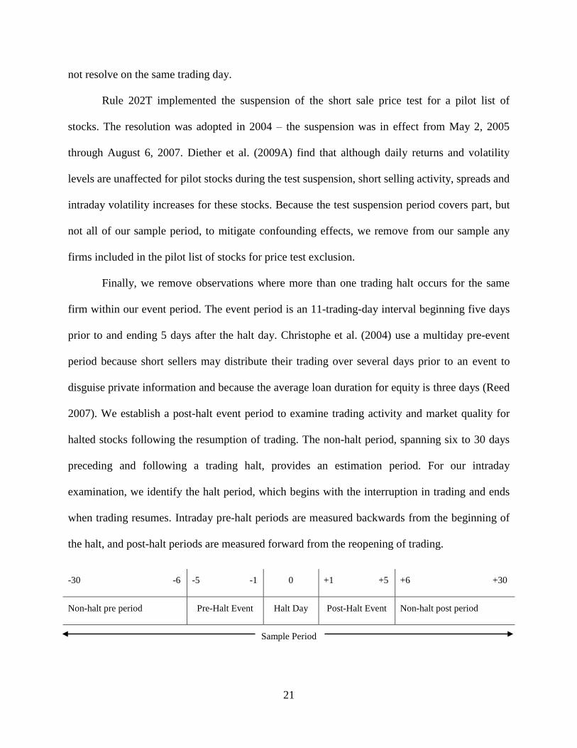
Finally, we remove observations where more than one trading halt occurs for the same
firm within our event period. The event period is an 11-trading-day interval beginning five days
prior to and ending 5 days after the halt day. Christophe et al. (2004) use a multiday pre-event
period because short sellers may distribute their trading over several days prior to an event to
disguise private information and because the average loan duration for equity is three days (Reed
2007). We establish a post-halt event period to examine trading activity and market quality for
halted stocks following the resumption of trading. The non-halt period, spanning six to 30 days
preceding and following a trading halt, provides an estimation period. For our intraday
examination, we identify the halt period, which begins with the interruption in trading and ends
when trading resumes. Intraday pre-halt periods are measured backwards from the beginning of
the halt, and post-halt periods are measured forward from the reopening of trading.
-30 -6 -5 -1 0 +1 +5 +6 +30
Non-halt pre period Pre-Halt Event Halt Day Post-Halt Event Non-halt post period
Sample Period

22
Daily price, trading volume, return, and market capitalization data are obtained from the
CRSP database. The Regulation SHO database, which was created in response to Rule 202T,
provides trade size and time stamps for short-selling transactions. TAQ trade and quote data is
used to examine intraday activity. Trade data is filtered to remove observations that occur
outside of normal market hours, and transactions with a non-positive price, or a condition code
other than zero. Quote data is filtered to retain observations that occur within normal market
hours and have a positive bid or ask size, price and spread.
SUMMARY STATISTICS
After applying the previously described filters to refine our set of events, our remaining
sample consists of 78 trading halts, 55 of which occur on the NYSE. Summary statistics
describing these halts are presented in Table 1, Panels A through I. Firm names, trading halt
mode and SIC code are listed in the Appendix E.
Table 1
Descriptive Statistics
This table contains summary statistics for trading halts that occur during 2005 – 2006 for NYSE-
listed firms. Halts have been filtered to remove observations that occur outside of market hours
or before 10:00 a.m., where more than one halt occurs for a sample firms on the same day, halts
that do not resolve on the same trading day and multiple halts for the same firm within the 11-
day event period, halts for Rule 202T pilot stocks, and observations for stocks whose average
daily price and trading volume during 2005 – 2006 was less than five dollars and 100 shares.
Panel A: Halts by Year
Year Number of Halts Unique Firms
2005 48 44
2006 30 28
Full Sample 78 68
Panel B: Number of Halts per Year
Number of Halts in Sample 1 2 3 4 5
Number of Firms
2005 42 1 0 1 0
2006 27 0 1 0 0
Full Sample 64 1 1 1 1
23
Panel C: Halts by Day of Week and Year
Day of Week
Year Monday Tuesday Wednesday Thursday Friday Total
2005 2 10 13 18 5 48
2006 4 9 7 5 5 30
Full Sample 6 19 20 23 10 78
Panel D: Halts by Month and Year
Month
Year Jan Feb March April May June July Aug Sep Oct Nov Dec
2005 4 2 5 7 8 5 4 5 1 3 2 2
2006 1 2 4 4 1 3 0 3 1 5 3 3
Full Sample 5 4 9 11 9 8 4 8 2 8 5 5
Panel E: Halts and Duration by Halt Type
Trading Halt Type Number of Halts Mean Duration
News Dissemination (4) 6 0:29:27
Order Imbalance (7) 7 0:17:29
News Pending (11) 65 0:44:46
Full Sample 78 0:41:08
Panel F: Halt Firm Characteristics - Average Daily Values
Price Volume Return Market Cap
Year: 2005 (N =44)
Mean 31.89 735,803 0.0590% 3,880,142
Max 110.65 5,902,434 0.3331% 65,755,430
Min 4.47 1099 -0.1728% 33,149
Std 23.90 1,295,571 0.1144% 10,371,325
Year: 2006 (N=28)
Mean 33.23 1,408,912 0.0438% 4,946,224
Max 141.33 7,642,372 0.3072% 40,548,995
Min 6.45 1,187 -0.4135% 111,400
Std 27.81 1,856,984 0.1346% 9,403,555
Full Sample (N=72)
Mean 32.41 997,568 0.0531% 4,294,729
Max 141.33 7,642,372 0.3331% 65,755,430
Min 4.47 1099 -0.4135% 33,149
Std 25.31 1,561,124 0.1219% 9,952,168
Panel G: CRSP Capitalization-Based Decile
Decile 2005 2006 Full Sample
1 0 0 0
2 2 0 2
3 4 2 6
4 4 1 5
5 5 2 7
6 6 8 14
24
7 2 3 5
8 9 4 13
9 4 3 7
10 8 5 13
Total 44 28 72
Panel H: Short-sale Trading Activity Across Exchanges (2005 – 2006)
ADF AMEX ARCA BSE CHX NASDAQ NSX NYSE PHLX
Mean Shares
Sold Short (%)
0.00 2.94 0.00 0.53 0.00 14.19 5.67 76.38 0.29
Mean Short-
sale Trades (%)
0.00 3.73 0.00 0.64 0.00 12.77 6.77 76.07 0.03
Panel I: Short-selling Summary Statistics per Stock
Mean Median Std Dev Minimum Maximum
Short Sale Daily Volume 201,427 192,125 72,895 67,124 1,285,773
Number of Daily Short Trades 379 349 149 128 2,727
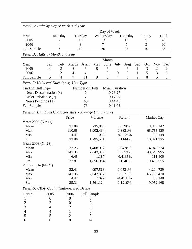
Of these halts, sixty percent more occur in 2005 than in 2006 (48 as compared to 30).
Similar to Christophe et al. (2004), we find that trading halts in our sample occur more
frequently during the middle of the week – Tuesday through Thursday. These interruptions in
trading occur in 23 out of the 24 sample period months, without evidence of an obvious seasonal
pattern. We examine 68 unique firms, 64 of which experience a single halt during the sample
period, and 4 different firms that experience 2, 3, 4, or 5 halts each.
The halts in our study are primarily (83 percent) implemented due to pending news. The
mean duration of all sample halts is just over 41 minutes. Although the duration of trading halts
reported by Lee et al. (1994), Corwin and Lipson (2000), and Christie, Corwin, and Harris
(2002) is greater on average and for each halt type, our findings coincide with previous research
in the ranking of halt types by length: news pending halts have the longest duration and order
imbalance halts, the shortest.
Summary statistics suggest a substantial variation in the size of sample firms, stock price
and trading volume with higher average values in 2006 as compared to 2005. The firms in our
25
study generally demonstrate positive returns over the two-year period examined. When the
sample firms are categorized according to year-end capitalization portfolio assignments
established by CRSP, we find, similar to Christophe et al. (2004) that large firms are more
heavily represented in our sample - we have fewer firms in the lower market capitalization
deciles. The dearth of smaller firms may be due, in part, to our data filter that eliminates trading
halts for any stock whose average daily price during the sample period is less than five dollars.
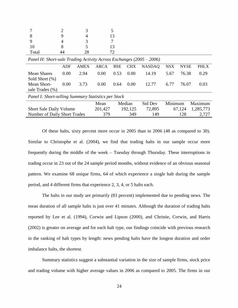
We examine short-selling levels for our sample firms during the 2005 – 2006 sample
period. For each exchange, we report both short volume as a percentage of the total shares
shorted and the number of short sale transactions as a percentage of the total number of short
selling trades. No short transactions for our sample firms/period are reported on the National
Association of Securities Dealers Alternative Display Facility (ADF), Archipelago (ARCA) and
the Chicago Stock Exchange (CHX).
In line with the findings presented by Diether et al. (2009B), approximately three-fourths
of short volume and short trades for our sample firms are executed on the NYSE. Approximately
14 percent of short volume and 13 percent of short trades are placed on the NASDAQ market.
The average firm in our sample has 379 short transactions per trading day with an average daily
short volume of just over 200,000 shares.
25
RESULTS
Daily Short Metrics
To describe the daily behavior of short sellers surrounding trading halts, we track the
mean number of trades, trade size and volume for short transactions for our sample firms in the
pre-event period (days -5 through -1), the halt day (day 0), the post-event period (days +1
through +5), and the estimation period (days -30 through -6 and +6 through +30). We also
calculate the short interest ratio, relative short selling, and abnormal short selling metrics for
each of these periods. The short interest ratio is the number of shares sold short to shares
outstanding (Angel et al., 2003). Relative short selling is computed by dividing the number of
shares shorted by the number of shares traded (Christophe et al., 2004; and Diether et al.,
2009B). Abnormal short selling is the percentage difference between the average daily shares
sold short during the pre, post or event period and the average daily number of shares sold short
during the estimation period (Lee et al., 1994; Corwin and Lipson, 2000; Christie et al., 2002,
Christophe et al., 2004; and Christophe et al., 2010).
Our hypotheses concerning the behavior of short sellers surrounding trading halts are:
H1: Prior to a trading halt, halted stocks will experience a substantial increase in the number
of short transactions, short sellers will utilize larger trade sizes and halted stocks will
experience a substantial increase in their short interest ratio, relative short selling, and
abnormal short selling measures.
26
H2: Following the resumption of trading, halted stocks will experience a substantial
decrease in the number of short transactions, short sellers will utilize smaller trade sizes
and halted stocks will experience a substantial decrease in their short interest ratio,
relative short selling, and abnormal short selling measures.
The mean daily short number of trades, trade size and trading volume, presented in Table
2, are lower in the pre-event period than in the estimation period, indicating that short sellers do
not increase their activity in the days prior to a trading halt. For example, the firms in our sample
had an average of 431 trades of 430 shares each, producing a mean short volume of 255,325
shares in the pre-event period. These values are all less than the corresponding mean expected
values computed for the estimation period. This finding, although in contrast to our priori, is
similar to the results of Christophe et al. (2004) who demonstrate a decrease in short selling
activity for firms during the five trading days preceding earnings announcements - another type
of informational event.
On the event day, all three of these metrics, number, size and total volume of short
transactions, increase dramatically. The average number of trades more than doubles, from 489
trades in the estimation period to over 1000 on the halt day. Trade size increases from 457 shares
to 646 and subsequently volume triples to an average of nearly one million shares sold short on
the halt day.
During the post-halt period, these values demonstrate a distinct reduction, but they
remain above estimation period levels. The mean number of daily short transactions falls from
1,004 to 662, which is substantially larger than estimated 489 trades; the average trade size of
477 shares remains elevated above the estimation size of 457 shares. The short interest ratio
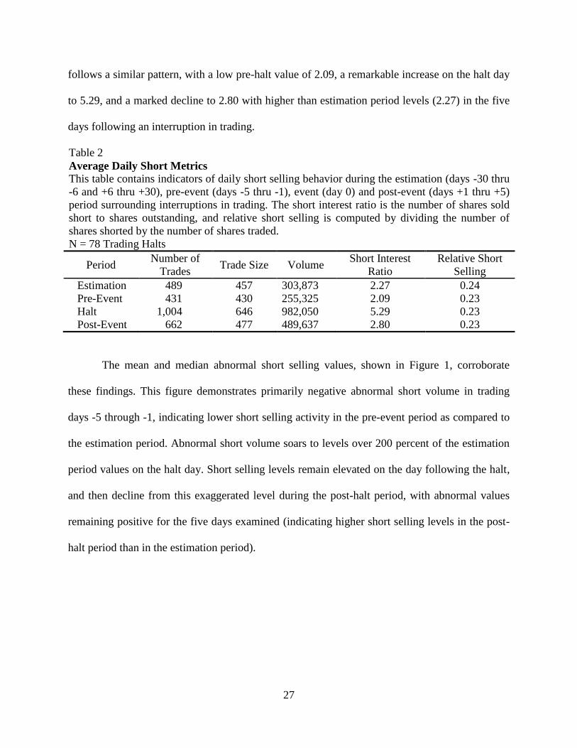
27
follows a similar pattern, with a low pre-halt value of 2.09, a remarkable increase on the halt day
to 5.29, and a marked decline to 2.80 with higher than estimation period levels (2.27) in the five
days following an interruption in trading.
Table 2
Average Daily Short Metrics
This table contains indicators of daily short selling behavior during the estimation (days -30 thru
-6 and +6 thru +30), pre-event (days -5 thru -1), event (day 0) and post-event (days +1 thru +5)
period surrounding interruptions in trading. The short interest ratio is the number of shares sold
short to shares outstanding, and relative short selling is computed by dividing the number of
shares shorted by the number of shares traded.
N = 78 Trading Halts
Period Number of
Trades Trade Size Volume
Short Interest
Ratio
Relative Short
Selling
Estimation 489 457 303,873 2.27 0.24
Pre-Event 431 430 255,325 2.09 0.23
Halt 1,004 646 982,050 5.29 0.23
Post-Event 662 477 489,637 2.80 0.23
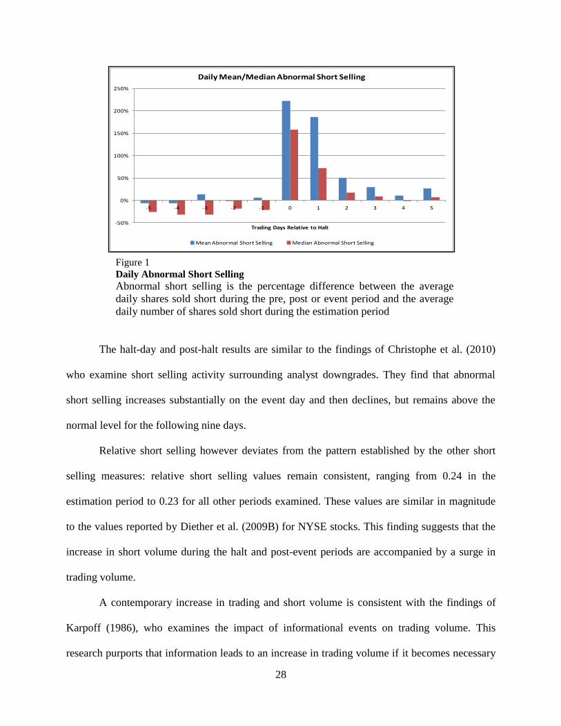
The mean and median abnormal short selling values, shown in Figure 1, corroborate
these findings. This figure demonstrates primarily negative abnormal short volume in trading
days -5 through -1, indicating lower short selling activity in the pre-event period as compared to
the estimation period. Abnormal short volume soars to levels over 200 percent of the estimation
period values on the halt day. Short selling levels remain elevated on the day following the halt,
and then decline from this exaggerated level during the post-halt period, with abnormal values
remaining positive for the five days examined (indicating higher short selling levels in the post-
halt period than in the estimation period).
28
Figure 1
Daily Abnormal Short Selling
Abnormal short selling is the percentage difference between the average
daily shares sold short during the pre, post or event period and the average
daily number of shares sold short during the estimation period
The halt-day and post-halt results are similar to the findings of Christophe et al. (2010)
who examine short selling activity surrounding analyst downgrades. They find that abnormal
short selling increases substantially on the event day and then declines, but remains above the
normal level for the following nine days.
Relative short selling however deviates from the pattern established by the other short
selling measures: relative short selling values remain consistent, ranging from 0.24 in the
estimation period to 0.23 for all other periods examined. These values are similar in magnitude
to the values reported by Diether et al. (2009B) for NYSE stocks. This finding suggests that the
increase in short volume during the halt and post-event periods are accompanied by a surge in
trading volume.
A contemporary increase in trading and short volume is consistent with the findings of
Karpoff (1986), who examines the impact of informational events on trading volume. This
research purports that information leads to an increase in trading volume if it becomes necessary
-50%
0%
50%
100%
150%
200%
250%
-5 -4 -3 -2 -1 0 1 2 3 4 5
Trading Days Relative to Halt
Daily Mean/Median Abnormal Short Selling
Mean Abnormal Short Selling Median Abnormal Short Selling
29
for investors to update their demand prices or if the information is not anticipated. Investor
disagreement or a divergence in investor expectations can lead to increased trading volume that
can persist after an informational event. Accordingly, Lee et al. (1994) report that trading volume
is 230 percent higher following NYSE trading halts as compared to levels following a ‘pseudo
halt’ and that the elevated volume persists for three days.
If informed short sellers are able to anticipate both that a firm will experience an
informational event and that this event will lead to a change in firm value, then we should expect
abnormal short selling to increase prior to interruptions in trading. Using the following equation,
we examine short selling levels while controlling for other variables that influence short selling
levels (following Christophe et al., 2010):
ABSS(-5,-1)i = αi + β1P(0i) + β2CAR(-5,-1)i + β3MOMi + β4CAR(0,1)i + εi (1)
The dependent variable, ABSS(-5,-1) represents abnormal short-selling during the five days
preceding the halt. P(0) is the share price of the halted firm on the halt day; this variable controls
for the positive link between a stock’s price and the willingness of market participants to short
the stock.4 CAR(-5,-1) is the cumulative abnormal return during the five day pre-event period – the
halted firm’s total return over the five days preceding the halt minus the median five-day
cumulative total return during the non-event period. MOM represents momentum, which
controls for long-term share price movement. Momentum is calculated as the halted firm’s six-
month cumulative return ending 30 days before the halt minus the return on the NYSE equally
weighted portfolio during the same period. CAR(0,1) is the halted firm’s holding period return
4 Refer to D’Avolio, (2002) who shows that the majority of stocks that are impossible to short are priced less than
five dollars and that the holdings of institutional investors, who lend stocks for shorting, are biased towards large,
liquid stocks.
30
from day 0 to day 1 minus the median holding period return during the non-event period; this
variable represents the market’s assessment of the economic value of the news released
surrounding a trading halt.
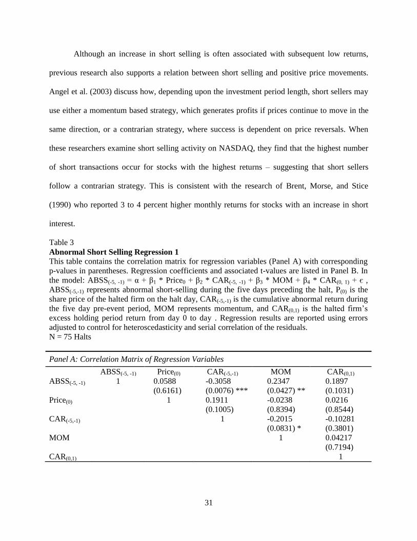
Table 3, Panel A presents the correlation matrix for the regression variables. Results
indicate that the pre-halt abnormal short selling level, ABSS(-5, -1), is significantly negatively
correlated with short-term pre-halt returns (CAR(-5, -1)) and significantly positively correlated
with long-term returns (MOM) prior to the trading halt. The correlation values indicates that pre-
event short selling decreases with high contemporaneous returns, but increases for stocks with
higher returns in the months prior to a trading halt.
Modeling a regression using ordinary least squares assumes that the error terms have
uniform variances across all observations. To ensure that this assumption holds, we test each
input data set using the Shapiro-Wilk test. The null hypothesis for this statistical test is that a
population is distributed normally. If the test produces a p-value less than the designated alpha
level, then the null hypothesis of normality can be rejected.
For this regression, the Shapiro-Wilk statistic is 0.73, with a p-value < .001, allowing us
to reject the assumption of a normal distribution. Accordingly, we execute our regression and
report results using errors adjusted to control for heteroscedasticity and serial correlation of the
residuals.
Table 3, Panel B presents the regression results. We find that the level of abnormal short
selling preceding a trading halt is positively associated with post-halt returns, CAR(0,1),
suggesting that for a stock with a 1 percent increase in post-halt returns we expect a 2 to 3
percent increase in pre-halt abnormal short selling.
31
Although an increase in short selling is often associated with subsequent low returns,
previous research also supports a relation between short selling and positive price movements.
Angel et al. (2003) discuss how, depending upon the investment period length, short sellers may
use either a momentum based strategy, which generates profits if prices continue to move in the
same direction, or a contrarian strategy, where success is dependent on price reversals. When
these researchers examine short selling activity on NASDAQ, they find that the highest number
of short transactions occur for stocks with the highest returns – suggesting that short sellers
follow a contrarian strategy. This is consistent with the research of Brent, Morse, and Stice
(1990) who reported 3 to 4 percent higher monthly returns for stocks with an increase in short
interest.
Table 3
Abnormal Short Selling Regression 1
This table contains the correlation matrix for regression variables (Panel A) with corresponding
p-values in parentheses. Regression coefficients and associated t-values are listed in Panel B. In
the model: ABSS(-5, -1) = α + β1 * Price0 + β2 * CAR(-5, -1) + β3 * MOM + β4 * CAR(0, 1) + є ,
ABSS(-5,-1) represents abnormal short-selling during the five days preceding the halt, P(0) is the
share price of the halted firm on the halt day, CAR(-5,-1) is the cumulative abnormal return during
the five day pre-event period, MOM represents momentum, and CAR(0,1) is the halted firm’s
excess holding period return from day 0 to day . Regression results are reported using errors
adjusted to control for heteroscedasticity and serial correlation of the residuals.
N = 75 Halts
Panel A: Correlation Matrix of Regression Variables
ABSS(-5, -1) Price(0) CAR(-5,-1) MOM CAR(0,1)
ABSS(-5, -1) 1 0.0588
(0.6161)
-0.3058
(0.0076) ***
0.2347
(0.0427) **
0.1897
(0.1031)
Price(0) 1 0.1911
(0.1005)
-0.0238
(0.8394)
0.0216
(0.8544)
CAR(-5,-1) 1 -0.2015
(0.0831) *
-0.10281
(0.3801)
MOM 1 0.04217
(0.7194)
CAR(0,1) 1
32
Panel B: OLS Regression Results
[1] [2] [3] [4]
Intercept 0.0054 (0.07) 0.0218 (0.25) -0.0019 (-0.02) -0.1203 (-0.91)
CAR(-5,-1) -3.7378 (-1.22) -3.5368 (-1.26) -3.1058 (-1.27) -3.3786 (-1.39)
CAR(0,1) 3.0178 (1.78) * 2.9454 (1.88) * 2.8576 (1.89) *
MOM 68.6249 (1.66) 67.9963 (1.67) *
Price(0) 0.0037 (1.12)
R2 0.0935 0.1188 0.1488 0.1610
Adjusted R2 0.0811 0.0943 0.1129 0.1131
F-Value 7.53 *** 4.85 ** 4.14 *** 3.36 **
***, **, and * indicate statistical significance at the 0.01, 0.05 and 0.10 level respectively.
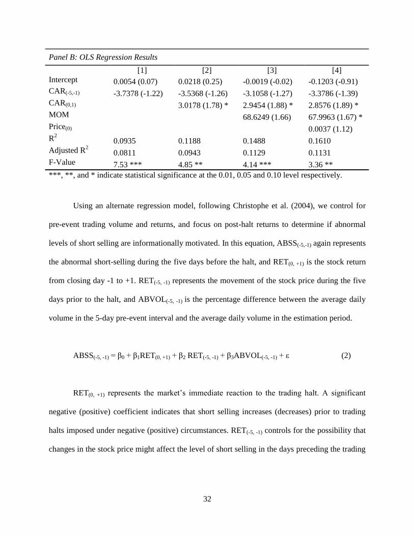
Using an alternate regression model, following Christophe et al. (2004), we control for
pre-event trading volume and returns, and focus on post-halt returns to determine if abnormal
levels of short selling are informationally motivated. In this equation, ABSS(-5,-1) again represents
the abnormal short-selling during the five days before the halt, and RET(0, +1) is the stock return
from closing day -1 to +1. RET(-5, -1) represents the movement of the stock price during the five
days prior to the halt, and ABVOL(-5, -1) is the percentage difference between the average daily
volume in the 5-day pre-event interval and the average daily volume in the estimation period.
ABSS(-5, -1) = β0 + β1RET(0, +1) + β2 RET(-5, -1) + β3ABVOL(-5, -1) + ε (2)
RET(0, +1) represents the market’s immediate reaction to the trading halt. A significant
negative (positive) coefficient indicates that short selling increases (decreases) prior to trading
halts imposed under negative (positive) circumstances. RET(-5, -1) controls for the possibility that
changes in the stock price might affect the level of short selling in the days preceding the trading
33
halt. ABVOL(-5, -1) accounts for the comovement in increased short selling activity and increased
trading volume (increased volume might make a stock easier to short).
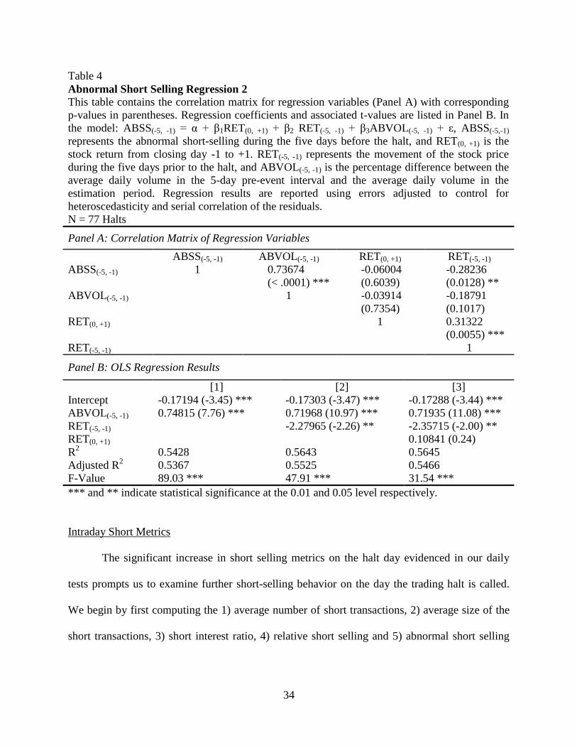
The correlation matrix of regression variables (Table 4 Panel A) demonstrates a
significant positive correlation between pre-halt abnormal short selling levels and abnormal
volume in the pre-halt period, suggesting that abnormal trading volume is linked to higher short
selling activity. 5
Pre-event abnormal short selling is negatively correlated with pre-halt returns –
stocks with higher return in the five days preceding a trading halt have lower levels of pre-halt
shorting.
For this regression, the Shapiro-Wilk statistic is 0.79, with a corresponding p-value <
.001. Accordingly, we execute our regression and report results using errors adjusted to control
for heteroscedasticity and serial correlation of the residuals.
The regression results, listed in Table 4 Panel B, produce relatively high Adjusted R2
values, ranging from 31.54 to 89.03 percent depending on the model specification. A significant
relation is indicated between abnormal short selling and trading volume and return in the pre-halt
period: pre-halt short selling levels are affected positively by stock price declines and by
increased trading volume in the days preceding a trading halt. These results indicate that a stock
with a one percent decrease (increase) in pre-halt returns (trading volume) we expect
approximately a (0.70) two percent increase in pre-halt abnormal short selling. However, the
coefficient for return over the halt day, RET(0, +1), is insignificant; this result fails to provide
support for our hypothesis of informed trading by short sellers prior to a trading halt.
5 Bris (2008) finds that short-sales ratios are affected by substantial increases in trading volume
34
Intraday Short Metrics
The significant increase in short selling metrics on the halt day evidenced in our daily
tests prompts us to examine further short-selling behavior on the day the trading halt is called.
We begin by first computing the 1) average number of short transactions, 2) average size of the
short transactions, 3) short interest ratio, 4) relative short selling and 5) abnormal short selling
Table 4
Abnormal Short Selling Regression 2
This table contains the correlation matrix for regression variables (Panel A) with corresponding
p-values in parentheses. Regression coefficients and associated t-values are listed in Panel B. In
the model: ABSS(-5, -1) = α + β1RET(0, +1) + β2 RET(-5, -1) + β3ABVOL(-5, -1) + ε, ABSS(-5,-1)
represents the abnormal short-selling during the five days before the halt, and RET(0, +1) is the
stock return from closing day -1 to +1. RET(-5, -1) represents the movement of the stock price
during the five days prior to the halt, and ABVOL(-5, -1) is the percentage difference between the
average daily volume in the 5-day pre-event interval and the average daily volume in the
estimation period. Regression results are reported using errors adjusted to control for
heteroscedasticity and serial correlation of the residuals.
N = 77 Halts
Panel A: Correlation Matrix of Regression Variables
ABSS(-5, -1) ABVOL(-5, -1) RET(0, +1) RET(-5, -1)
ABSS(-5, -1) 1 0.73674
(< .0001) ***
-0.06004
(0.6039)
-0.28236
(0.0128) **
ABVOL(-5, -1) 1 -0.03914
(0.7354)
-0.18791
(0.1017)
RET(0, +1) 1 0.31322
(0.0055) ***
RET(-5, -1) 1
Panel B: OLS Regression Results
[1] [2] [3]
Intercept -0.17194 (-3.45) *** -0.17303 (-3.47) *** -0.17288 (-3.44) ***
ABVOL(-5, -1) 0.74815 (7.76) *** 0.71968 (10.97) *** 0.71935 (11.08) ***
RET(-5, -1) -2.27965 (-2.26) ** -2.35715 (-2.00) **
RET(0, +1) 0.10841 (0.24)
R2 0.5428 0.5643 0.5645
Adjusted R2 0.5367 0.5525 0.5466
F-Value 89.03 *** 47.91 *** 31.54 ***
*** and ** indicate statistical significance at the 0.01 and 0.05 level respectively.

35
measures for the halted stocks in the eight 30-minute periods prior to a halt and following the
resumption of trading.
Our investigation reveals that the number of trades, the transaction size, the overall short
volume and the short interest ratio remain relatively stable throughout the periods leading up to
the halt (Table 5). The pre-halt short interest ratio varies from 0.162 to 0.313. The number of
short transactions ranges from 59 to 94 per period and mean period trade size is between 544 and
841 shares, producing short volume for the pre-halt periods ranging from 36,795 to 65,965
shares. A slight increase in pre-halt short activity, with volume breaching 60,000, is noted two
periods preceding the halt.
Table 5
Average Intraday Short Metrics
Mean values, which are computed for eight 30-minute periods prior to trading halts and
following the resumption of trading, are on a per halt basis; they are adjusted for the number of
halts with short transactions each period. The short interest ratio is the number of shares sold
short to shares outstanding, and relative short selling is computed by dividing the number of
shares shorted by the number of shares traded.
Period Number
of Halts
Number of
Trades Trade Size Volume
Short Interest
Ratio
Relative Short
Selling
-8 21 94 692 65,338 0.313 0.259
-7 25 83 544 45,241 0.163 0.203
-6 32 59 628 36,795 0.185 0.240
-5 43 81 704 56,985 0.311 0.242
-4 49 63 613 38,790 0.162 0.220
-3 50 66 792 52,046 0.294 0.242
-2 55 73 841 61,604 0.207 0.247
-1 61 87 757 65,965 0.220 0.245
Halt
1 68 162 1,293 209,182 1.601 0.238
2 56 120 1,126 135,328 0.777 0.223
3 53 99 855 84,429 0.611 0.253
4 43 63 998 63,200 0.472 0.286
5 38 76 1,011 77,129 0.560 0.288
6 32 81 1,145 92,495 0.479 0.266
7 25 93 1,191 111,295 0.363 0.266
8 14 31 339 10,470 0.236 0.245
36
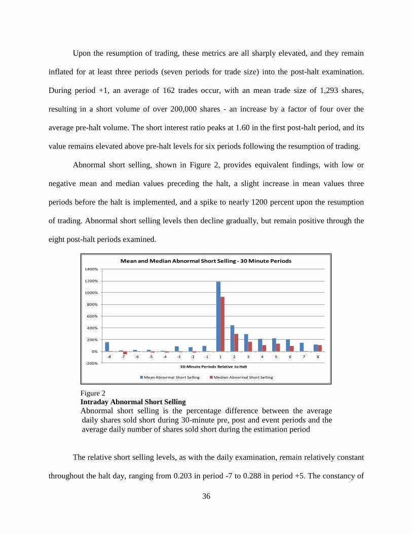
Upon the resumption of trading, these metrics are all sharply elevated, and they remain
inflated for at least three periods (seven periods for trade size) into the post-halt examination.
During period +1, an average of 162 trades occur, with an mean trade size of 1,293 shares,
resulting in a short volume of over 200,000 shares - an increase by a factor of four over the
average pre-halt volume. The short interest ratio peaks at 1.60 in the first post-halt period, and its
value remains elevated above pre-halt levels for six periods following the resumption of trading.
Abnormal short selling, shown in Figure 2, provides equivalent findings, with low or
negative mean and median values preceding the halt, a slight increase in mean values three
periods before the halt is implemented, and a spike to nearly 1200 percent upon the resumption
of trading. Abnormal short selling levels then decline gradually, but remain positive through the
eight post-halt periods examined.
Figure 2
Intraday Abnormal Short Selling
Abnormal short selling is the percentage difference between the average
daily shares sold short during 30-minute pre, post and event periods and the
average daily number of shares sold short during the estimation period
The relative short selling levels, as with the daily examination, remain relatively constant
throughout the halt day, ranging from 0.203 in period -7 to 0.288 in period +5. The constancy of
-200%
0%
200%
400%
600%
800%
1000%
1200%
1400%
-8 -7 -6 -5 -4 -3 -2 -1 1 2 3 4 5 6 7 8
30-Minute Periods Relative to Halt
Mean and Median Abnormal Short Selling - 30 Minute Periods
Mean Abnormal Short Selling Median Abnormal Short Selling

37
the relative short selling ratio suggests that elevated short selling levels are accompanied by
corresponding increases in trading volume. To explore further, we plot both short selling and
trading volume for our sample firms across the halt day. The graphic produced, Figure 3, depicts
a contemporaneous increase in both trading and short selling volume immediately preceding the
halt, peaking upon the continuation of trading and remaining elevated for several periods post-
halt. This pattern coincides with significant increases in trading volume reported by Christie et
al. (2002) one period preceding and several periods following the resumption of trade for a
sample of NASDAQ firms experiencing a trading halt.
Figure 3
Halt Day Trading and Short Selling Volume
The results of our empirical investigation do not provide solid support for Hypothesis 1.
Although an increase in each of the metrics we used to describe short seller behavior was
anticipated during the pre-halt period, we found instead, at the daily level, that short selling
activity did not increase substantially prior to the implementation of a trading halt. Our intraday
examination provides evidence of only a modest increase in short selling immediately preceding
an interruption in trading.
-
200,000
400,000
600,000
800,000
1,000,000
1,200,000
-8 -7 -6 -5 -4 -3 -2 -1 1 2 3 4 5 6 7 8
Shar
es
30-Minute Periods Relative to Trading Halt
Halt Day Trading and Short Selling Volume Per Period
Short Selling Volume
Trading Volume

38
However, it does appear that short sellers significantly modify their behavior surrounding
trading halts, as each of our short metrics, with the exception of relative short selling,
demonstrates substantial increases on the event day, upon the resumption of trading. Support is
provided for Hypothesis 2; average trade size, number of trades and volume for short
transactions, short interest ratio and abnormal short selling all decrease markedly in the post-
event period.
Daily Return Behavior
We next turn our investigation to the price behavior of stocks experiencing a trading halt
by examining daily post-halt prices and subsequent returns. To help quantify the impact of short
selling, we sort sample halts into quintiles according to mean pre-halt abnormal short selling
(ABSS) and abnormal relative short selling (ABRELSS) levels. Abnormal relative short selling
is calculated by subtracting the estimation period relative short selling from the relative short
selling in the pre-halt period. We examine and report, in Table 6, daily mean and median post-
announcement returns (each stock’s two-day percentage return following the trading halt,
measured from the close of the day preceding the halt day to the close of the following day) for
the highest and lowest quintiles (following Christophe et al. 2004).
Our hypothesis concerning the return earned by sample firms surrounding interruptions in
trading states that:
H3: Halted stocks with high levels of short selling will experience a larger decline in price
surrounding a trading halt as compared to halted stocks with lower short selling
activity.
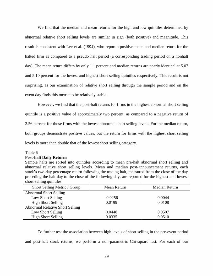
39
We find that the median and mean returns for the high and low quintiles determined by
abnormal relative short selling levels are similar in sign (both positive) and magnitude. This
result is consistent with Lee et al. (1994), who report a positive mean and median return for the
halted firm as compared to a pseudo halt period (a corresponding trading period on a nonhalt
day). The mean return differs by only 1.1 percent and median returns are nearly identical at 5.07
and 5.10 percent for the lowest and highest short selling quintiles respectively. This result is not
surprising, as our examination of relative short selling through the sample period and on the
event day finds this metric to be relatively stable.
However, we find that the post-halt returns for firms in the highest abnormal short selling
quintile is a positive value of approximately two percent, as compared to a negative return of
2.56 percent for those firms with the lowest abnormal short selling levels. For the median return,
both groups demonstrate positive values, but the return for firms with the highest short selling
levels is more than double that of the lowest short selling category.
Table 6
Post-halt Daily Returns
Sample halts are sorted into quintiles according to mean pre-halt abnormal short selling and
abnormal relative short selling levels. Mean and median post-announcement returns, each
stock’s two-day percentage return following the trading halt, measured from the close of the day
preceding the halt day to the close of the following day, are reported for the highest and lowest
short-selling quintiles
Short Selling Metric / Group Mean Return Median Return
Abnormal Short Selling
Low Short Selling -0.0256 0.0044
High Short Selling 0.0199 0.0108
Abnormal Relative Short Selling
Low Short Selling 0.0448 0.0507
High Short Selling 0.0335 0.0510
To further test the association between high levels of short selling in the pre-event period
and post-halt stock returns, we perform a non-parametric Chi-square test. For each of our

40
abnormal short selling metrics, ABSS and ABRELSS, we split the sample into two groups, the
highest quintile of each measure for days -5 thru -1, and all other sample halts. We then examine
how these groups are distributed across three categories of return from closing day -1 to +1. If
short selling is randomly dispersed the halts should have the following distribution: 20 percent in
the low return quintile, 20 percent in the high return quintile and 60 percent in the moderate
return quintile (following Dechow et al., 2001; and Christophe et al., 2004). Accordingly, with
77 trading halt observations, 15 observations each (approximately 19 percent) should fall into the
low and high return categories, and the remaining 47 observations (≈ 61 percent) should be
designated as moderate.
Table 7 presents these findings, with quintiles established according to ABSS and
RELABSS levels presented in Panel A and Panel B respectively. We find that the highest short-
selling quintile for ABSS has the anticipated 20 percent of its observations in the low return
category. However, nearly 27 percent of the halts in the highest short-selling quintile are
associated with high returns – this result coincides with our findings from Table 6 (positive
returns for high short selling stocks) and suggests that stocks with the highest levels of pre-halt
abnormal short selling have higher post-halt returns. The other short-selling quintile category
demonstrates a distribution that is in line with expected values.
When categorizing the stock according to levels of ABRELSS, we see a more
pronounced shift of the high short-selling stocks (40 percent) into the high return category with
the remaining short selling quintiles demonstrating a pattern similar to the expected values. The
ABRELSS Chi-Square test produces a X2 statistic that is significant at the 10 percent level,
which allows us to reject the null hypothesis of independence between short selling and post-
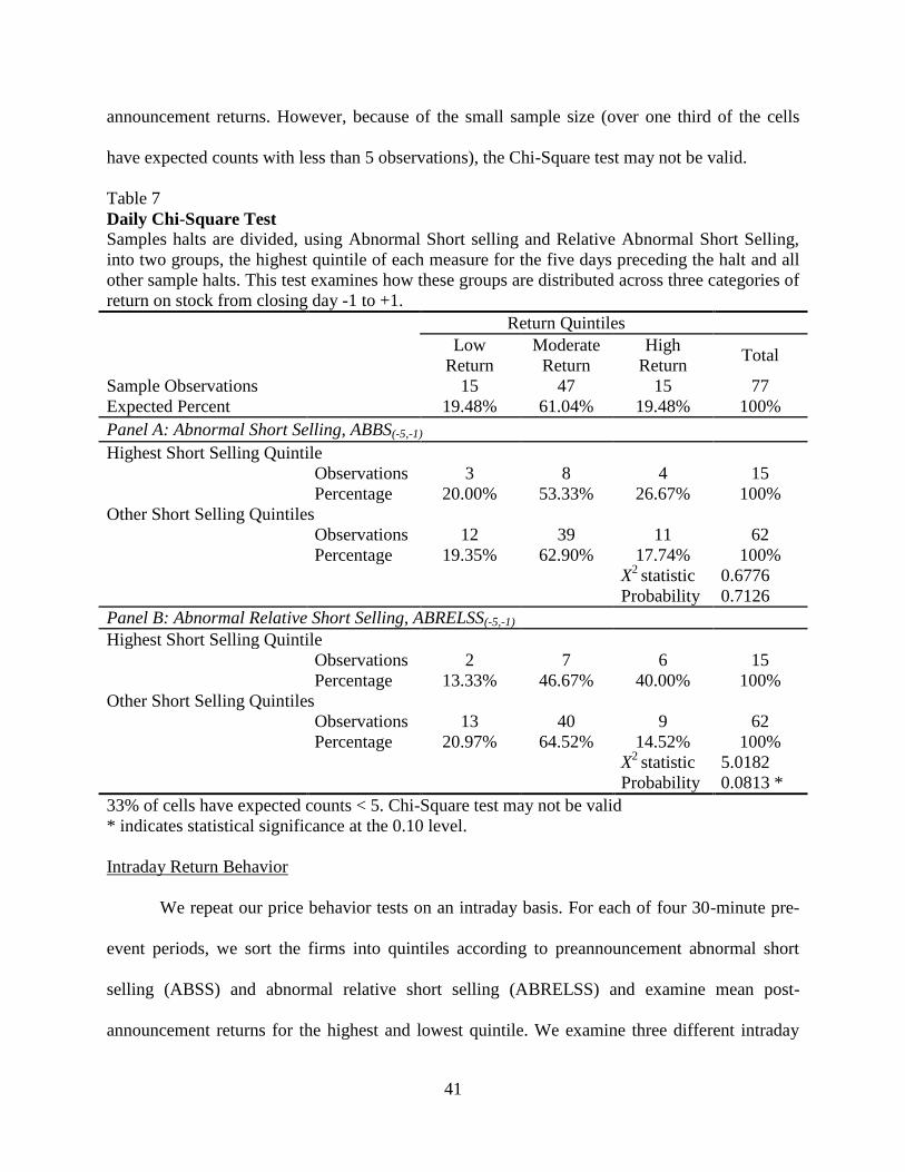
41
announcement returns. However, because of the small sample size (over one third of the cells
have expected counts with less than 5 observations), the Chi-Square test may not be valid.
Table 7
Daily Chi-Square Test
Samples halts are divided, using Abnormal Short selling and Relative Abnormal Short Selling,
into two groups, the highest quintile of each measure for the five days preceding the halt and all
other sample halts. This test examines how these groups are distributed across three categories of
return on stock from closing day -1 to +1.
Return Quintiles
Low
Return
Moderate
Return
High
Return Total
Sample Observations 15 47 15 77
Expected Percent 19.48% 61.04% 19.48% 100%
Panel A: Abnormal Short Selling, ABBS(-5,-1)
Highest Short Selling Quintile
Observations 3 8 4 15
Percentage 20.00% 53.33% 26.67% 100%
Other Short Selling Quintiles
Observations 12 39 11 62
Percentage 19.35% 62.90% 17.74% 100%
X2
statistic 0.6776
Probability 0.7126
Panel B: Abnormal Relative Short Selling, ABRELSS(-5,-1)
Highest Short Selling Quintile
Observations 2 7 6 15
Percentage 13.33% 46.67% 40.00% 100%
Other Short Selling Quintiles
Observations 13 40 9 62
Percentage 20.97% 64.52% 14.52% 100%
X2
statistic 5.0182
Probability 0.0813 *
33% of cells have expected counts < 5. Chi-Square test may not be valid
* indicates statistical significance at the 0.10 level.
Intraday Return Behavior
We repeat our price behavior tests on an intraday basis. For each of four 30-minute pre-
event periods, we sort the firms into quintiles according to preannouncement abnormal short
selling (ABSS) and abnormal relative short selling (ABRELSS) and examine mean post-
announcement returns for the highest and lowest quintile. We examine three different intraday
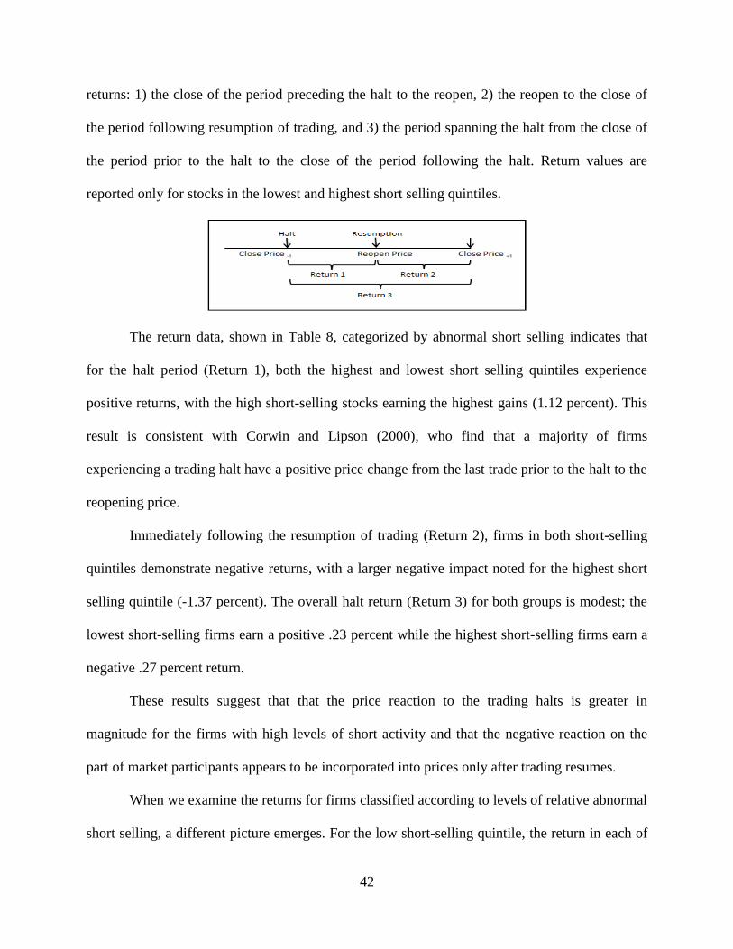
42
returns: 1) the close of the period preceding the halt to the reopen, 2) the reopen to the close of
the period following resumption of trading, and 3) the period spanning the halt from the close of
the period prior to the halt to the close of the period following the halt. Return values are
reported only for stocks in the lowest and highest short selling quintiles.
The return data, shown in Table 8, categorized by abnormal short selling indicates that
for the halt period (Return 1), both the highest and lowest short selling quintiles experience
positive returns, with the high short-selling stocks earning the highest gains (1.12 percent). This
result is consistent with Corwin and Lipson (2000), who find that a majority of firms
experiencing a trading halt have a positive price change from the last trade prior to the halt to the
reopening price.
Immediately following the resumption of trading (Return 2), firms in both short-selling
quintiles demonstrate negative returns, with a larger negative impact noted for the highest short
selling quintile (-1.37 percent). The overall halt return (Return 3) for both groups is modest; the
lowest short-selling firms earn a positive .23 percent while the highest short-selling firms earn a
negative .27 percent return.
These results suggest that that the price reaction to the trading halts is greater in
magnitude for the firms with high levels of short activity and that the negative reaction on the
part of market participants appears to be incorporated into prices only after trading resumes.
When we examine the returns for firms classified according to levels of relative abnormal
short selling, a different picture emerges. For the low short-selling quintile, the return in each of
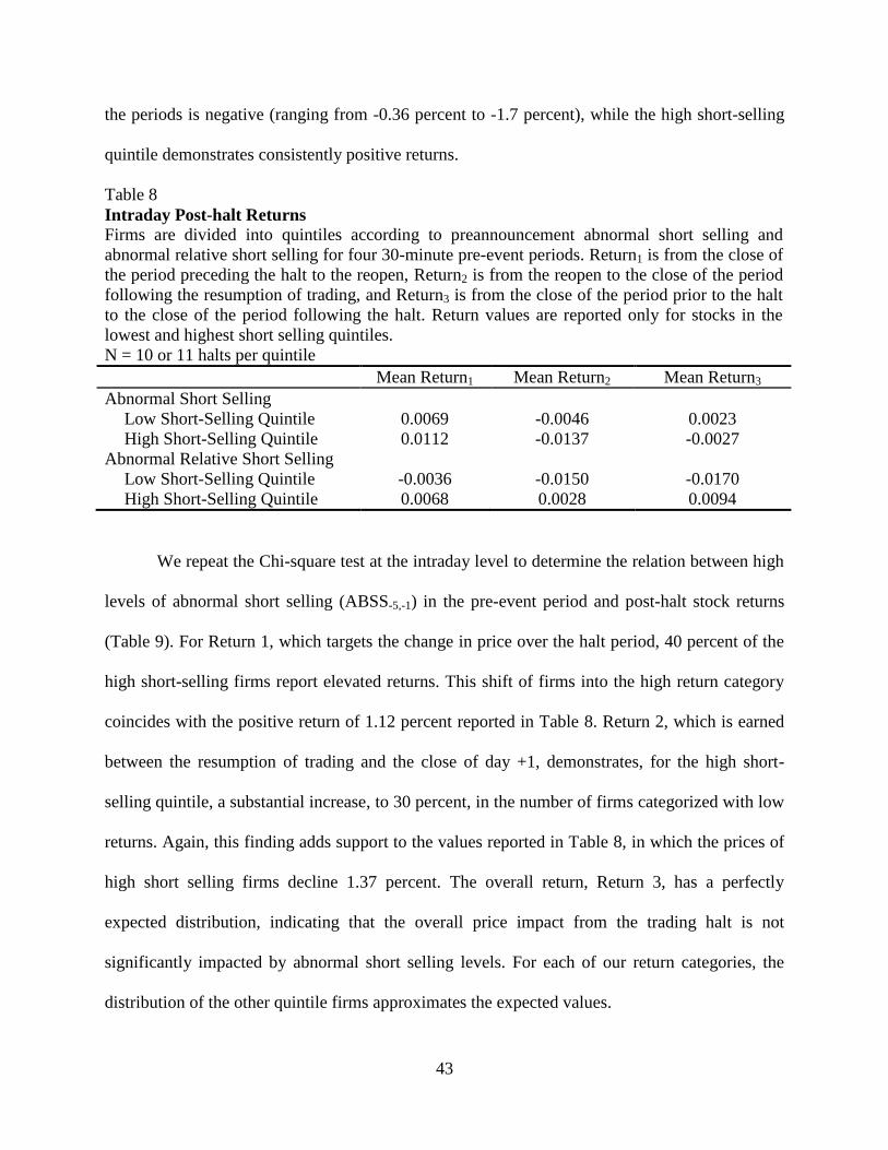
43
the periods is negative (ranging from -0.36 percent to -1.7 percent), while the high short-selling
quintile demonstrates consistently positive returns.
Table 8
Intraday Post-halt Returns
Firms are divided into quintiles according to preannouncement abnormal short selling and
abnormal relative short selling for four 30-minute pre-event periods. Return1 is from the close of
the period preceding the halt to the reopen, Return2 is from the reopen to the close of the period
following the resumption of trading, and Return3 is from the close of the period prior to the halt
to the close of the period following the halt. Return values are reported only for stocks in the
lowest and highest short selling quintiles.
N = 10 or 11 halts per quintile
Mean Return1 Mean Return2 Mean Return3
Abnormal Short Selling
Low Short-Selling Quintile 0.0069 -0.0046 0.0023
High Short-Selling Quintile 0.0112 -0.0137 -0.0027
Abnormal Relative Short Selling
Low Short-Selling Quintile -0.0036 -0.0150 -0.0170
High Short-Selling Quintile 0.0068 0.0028 0.0094
We repeat the Chi-square test at the intraday level to determine the relation between high
levels of abnormal short selling (ABSS-5,-1) in the pre-event period and post-halt stock returns
(Table 9). For Return 1, which targets the change in price over the halt period, 40 percent of the
high short-selling firms report elevated returns. This shift of firms into the high return category
coincides with the positive return of 1.12 percent reported in Table 8. Return 2, which is earned
between the resumption of trading and the close of day +1, demonstrates, for the high short-
selling quintile, a substantial increase, to 30 percent, in the number of firms categorized with low
returns. Again, this finding adds support to the values reported in Table 8, in which the prices of
high short selling firms decline 1.37 percent. The overall return, Return 3, has a perfectly
expected distribution, indicating that the overall price impact from the trading halt is not
significantly impacted by abnormal short selling levels. For each of our return categories, the
distribution of the other quintile firms approximates the expected values.
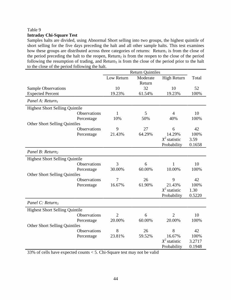
44
Table 9
Intraday Chi-Square Test
Samples halts are divided, using Abnormal Short selling into two groups, the highest quintile of
short selling for the five days preceding the halt and all other sample halts. This test examines
how these groups are distributed across three categories of returns: Return1 is from the close of
the period preceding the halt to the reopen, Return2 is from the reopen to the close of the period
following the resumption of trading, and Return3 is from the close of the period prior to the halt
to the close of the period following the halt.
Return Quintiles
Low Return Moderate
Return
High Return Total
Sample Observations 10 32 10 52
Expected Percent 19.23% 61.54% 19.23% 100%
Panel A: Return1
Highest Short Selling Quintile
Observations 1 5 4 10
Percentage 10% 50% 40% 100%
Other Short Selling Quintiles
Observations 9 27 6 42
Percentage 21.43% 64.29% 14.29% 100%
X2
statistic 3.59
Probability 0.1658
Panel B: Return2
Highest Short Selling Quintile
Observations 3 6 1 10
Percentage 30.00% 60.00% 10.00% 100%
Other Short Selling Quintiles
Observations 7 26 9 42
Percentage 16.67% 61.90% 21.43% 100%
X2
statistic 1.30
Probability 0.5220
Panel C: Return3
Highest Short Selling Quintile
Observations 2 6 2 10
Percentage 20.00% 60.00% 20.00% 100%
Other Short Selling Quintiles
Observations 8 26 8 42
Percentage 23.81% 59.52% 16.67% 100%
X2
statistic 3.2717
Probability 0.1948
33% of cells have expected counts < 5. Chi-Square test may not be valid

45
Diether et al. (2009B) provide insight into this return pattern: a sizeable negative return in
the immediate 30-minute post-halt period and a positive average daily post-halt return. These
researchers suggest that if short sellers increase their activity to provide liquidity at times when
buyers are willing to pay a premium for immediacy, then after an initial negative reaction, stock
prices will revert to normal levels when the buying pressure diminishes. Alternatively, if an
increased level of shorting activity is in response to liquidity demands in periods of heightened
uncertainty, due to either divergent opinions or informed trading, prices will return to normal
levels when the cause of the uncertainty is resolved.
Hypothesis 3 states that halted stocks with higher levels of short selling will experience a
larger decline in price surrounding a trading halt as compared to halted stocks without a
significant level of short selling. At the daily level, however, we find evidence of the opposite
effect – firms with higher shorting activity earn higher gains than do halted firms with lower short
selling levels. On an intraday basis, our findings suggest that firms with elevated levels of
shorting experience larger positive gains during the halt period and a substantial price decrease
immediately after trading resumes.
Speed of Price Adjustment
Short selling and trading halts both have the potential to convey information to market
participants, and thus affect the price discovery process. Accordingly, we investigate the rate at
which the price of our sample firms’ stock adjusts under the combined impact of these trading
activities.
Our hypothesis concerning the impact of short selling on stock prices surrounding trading
halts states:
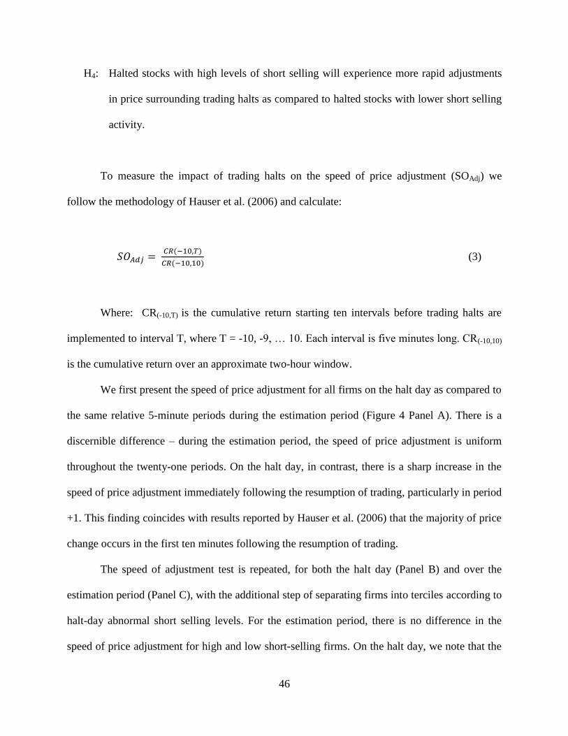
46
H4: Halted stocks with high levels of short selling will experience more rapid adjustments
in price surrounding trading halts as compared to halted stocks with lower short selling
activity.
To measure the impact of trading halts on the speed of price adjustment (SOAdj) we
follow the methodology of Hauser et al. (2006) and calculate:
(3)
Where: CR(-10,T) is the cumulative return starting ten intervals before trading halts are
implemented to interval T, where T = -10, -9, … 10. Each interval is five minutes long. CR(-10,10)
is the cumulative return over an approximate two-hour window.
We first present the speed of price adjustment for all firms on the halt day as compared to
the same relative 5-minute periods during the estimation period (Figure 4 Panel A). There is a
discernible difference – during the estimation period, the speed of price adjustment is uniform
throughout the twenty-one periods. On the halt day, in contrast, there is a sharp increase in the
speed of price adjustment immediately following the resumption of trading, particularly in period
+1. This finding coincides with results reported by Hauser et al. (2006) that the majority of price
change occurs in the first ten minutes following the resumption of trading.
The speed of adjustment test is repeated, for both the halt day (Panel B) and over the
estimation period (Panel C), with the additional step of separating firms into terciles according to
halt-day abnormal short selling levels. For the estimation period, there is no difference in the
speed of price adjustment for high and low short-selling firms. On the halt day, we note that the
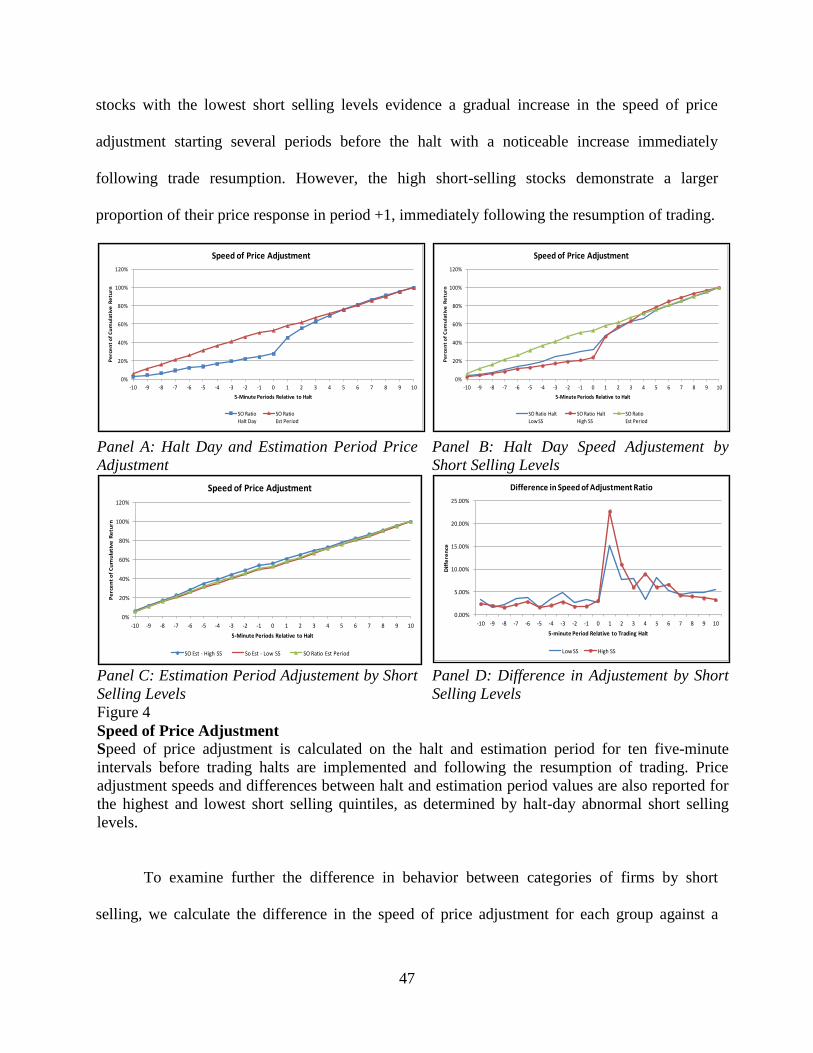
47
stocks with the lowest short selling levels evidence a gradual increase in the speed of price
adjustment starting several periods before the halt with a noticeable increase immediately
following trade resumption. However, the high short-selling stocks demonstrate a larger
proportion of their price response in period +1, immediately following the resumption of trading.
Panel A: Halt Day and Estimation Period Price
Adjustment
Panel B: Halt Day Speed Adjustement by
Short Selling Levels
Panel C: Estimation Period Adjustement by Short
Selling Levels
Panel D: Difference in Adjustement by Short
Selling Levels
Figure 4
Speed of Price Adjustment
Speed of price adjustment is calculated on the halt and estimation period for ten five-minute
intervals before trading halts are implemented and following the resumption of trading. Price
adjustment speeds and differences between halt and estimation period values are also reported for
the highest and lowest short selling quintiles, as determined by halt-day abnormal short selling
levels.
To examine further the difference in behavior between categories of firms by short
selling, we calculate the difference in the speed of price adjustment for each group against a
0%
20%
40%
60%
80%
100%
120%
-10 -9 -8 -7 -6 -5 -4 -3 -2 -1 0 1 2 3 4 5 6 7 8 9 10
Pe
rce
nt
of
Cu
mu
lati
ve
Re
turn
5-Minute Periods Relative to Halt
Speed of Price Adjustment
SO RatioHalt Day
SO RatioEst Period
0%
20%
40%
60%
80%
100%
120%
-10 -9 -8 -7 -6 -5 -4 -3 -2 -1 0 1 2 3 4 5 6 7 8 9 10
Pe
rce
nt
of
Cu
mu
lati
ve
Re
turn
5-Minute Periods Relative to Halt
Speed of Price Adjustment
SO Ratio HaltLow SS
SO Ratio HaltHigh SS
SO RatioEst Period
0%
20%
40%
60%
80%
100%
120%
-10 -9 -8 -7 -6 -5 -4 -3 -2 -1 0 1 2 3 4 5 6 7 8 9 10
Pe
rce
nt
of
Cu
mu
lati
ve
Re
turn
5-Minute Periods Relative to Halt
Speed of Price Adjustment
SO Est - High SS So Est - Low SS SO Ratio Est Period
0.00%
5.00%
10.00%
15.00%
20.00%
25.00%
-10 -9 -8 -7 -6 -5 -4 -3 -2 -1 0 1 2 3 4 5 6 7 8 9 10
Dif
fere
nce
5-minute Period Relative to Trading Halt
Difference in Speed of Adjustment Ratio
Low SS High SS

48
benchmark that assumes 4.76 percent of the price change occurs in each 5-minute period (100
percent / 21 periods). These results, shown in Figure 4 Panel D, suggest that stocks with high
levels of short selling demonstrate a larger increase in price adjustment than do stocks in the
lowest short selling group (23 percent as compared to 15 percent) in the periods immediately
following the resumption of trading.
Weighted Price Contribution
To investigate further the price discovery process for halted stocks, we identify the
cumulative price change at the daily and intraday level in each sample interval (pre-halt, halt,
post-halt) by calculating the weighted price contribution estimate, following Madura et al. 2006:
(4)
Where: i є each interval (pre-halt, halt, post-halt) and is the price change over
interval i for halt j.
As presented in Table 10, nearly 60 percent of the price contribution at the daily level
occurs on the halt day, with 28 percent occurring in the 5 days preceding the halt and only 11
percent in the post-halt period. This finding indicates that, although a significant price reaction
occurs prior to the trading halt event, the majority of the market’s reaction is confined to the halt
day. Our results are similar to those of Madura et al. (2006), who report the majority of price
change in the halt period (≈ 79 percent) and the least amount of price change in the post halt
period in their examination of NASDAQ trading halts.
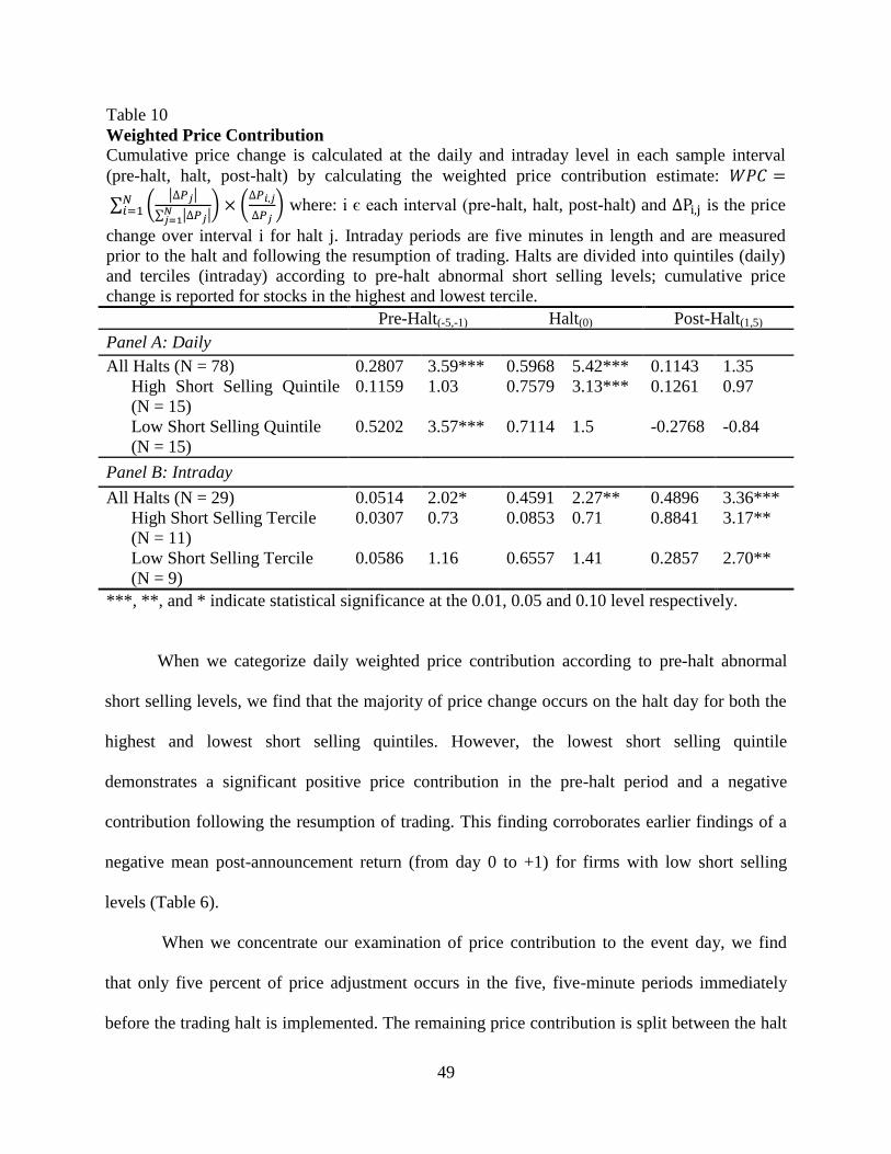
49
Table 10
Weighted Price Contribution
Cumulative price change is calculated at the daily and intraday level in each sample interval
(pre-halt, halt, post-halt) by calculating the weighted price contribution estimate:
where: i є each interval (pre-halt, halt, post-halt) and is the price
change over interval i for halt j. Intraday periods are five minutes in length and are measured
prior to the halt and following the resumption of trading. Halts are divided into quintiles (daily)
and terciles (intraday) according to pre-halt abnormal short selling levels; cumulative price
change is reported for stocks in the highest and lowest tercile.
Pre-Halt(-5,-1) Halt(0) Post-Halt(1,5)
Panel A: Daily
All Halts (N = 78) 0.2807 3.59*** 0.5968 5.42*** 0.1143 1.35
High Short Selling Quintile
(N = 15)
0.1159 1.03 0.7579 3.13*** 0.1261 0.97
Low Short Selling Quintile
(N = 15)
0.5202 3.57*** 0.7114 1.5 -0.2768 -0.84
Panel B: Intraday
All Halts (N = 29) 0.0514 2.02* 0.4591 2.27** 0.4896 3.36***
High Short Selling Tercile
(N = 11)
0.0307 0.73 0.0853 0.71 0.8841 3.17**
Low Short Selling Tercile
(N = 9)
0.0586 1.16 0.6557 1.41 0.2857 2.70**
***, **, and * indicate statistical significance at the 0.01, 0.05 and 0.10 level respectively.
When we categorize daily weighted price contribution according to pre-halt abnormal
short selling levels, we find that the majority of price change occurs on the halt day for both the
highest and lowest short selling quintiles. However, the lowest short selling quintile
demonstrates a significant positive price contribution in the pre-halt period and a negative
contribution following the resumption of trading. This finding corroborates earlier findings of a
negative mean post-announcement return (from day 0 to +1) for firms with low short selling
levels (Table 6).
When we concentrate our examination of price contribution to the event day, we find
that only five percent of price adjustment occurs in the five, five-minute periods immediately
before the trading halt is implemented. The remaining price contribution is split between the halt

50
period and the five periods following the resumption of trading. Segmenting our results
according to short selling levels confirms that only a small percentage of price contribution, three
to six percent, occurs directly preceding the trading halts. However, it appears that price behavior
is much different between firms with high and low levels of short selling. The majority, 88
percent, of price change for firms in the highest short selling tercile occurs in the post-halt
period. For firms in the lowest short selling tercile, the largest price contribution, 66 percent,
transpires while trading is halted.
Hypothesis 4 states that halted firms with high short selling will experience a more rapid
adjustment in price prior to a trading halt as compared to halted stocks without a significant level
of short selling. Our results, from both the speed of price adjustment and weighted price
contribution tests suggest that effect of the trading halt on equity prices is more pronounced
following the resumption of trading, not before the halt is implemented. However, both tests
indicate a discernible difference between firms according to short selling activity; a larger price
impact is reported in the post-halt period for stocks with the highest shorting levels.
Volatility
To explore the relation between trading halts and short selling activity, we examine, on
both the daily and intraday level, price volatility surrounding interruptions in trading.
Our hypothesis concerning the effect of short selling on price volatility for firms
experiencing a trading halt is:
H5: Halted stocks with high levels of short selling will have lower price volatility upon
resumption of trade and their reopening prices will be better predictors of future prices
as compared to halted stocks with lower short selling activity.
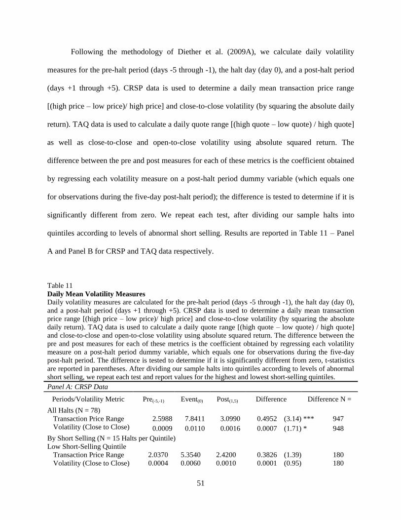
51
Following the methodology of Diether et al. (2009A), we calculate daily volatility
measures for the pre-halt period (days -5 through -1), the halt day (day 0), and a post-halt period
(days +1 through +5). CRSP data is used to determine a daily mean transaction price range
[(high price – low price)/ high price] and close-to-close volatility (by squaring the absolute daily
return). TAQ data is used to calculate a daily quote range [(high quote – low quote) / high quote]
as well as close-to-close and open-to-close volatility using absolute squared return. The
difference between the pre and post measures for each of these metrics is the coefficient obtained
by regressing each volatility measure on a post-halt period dummy variable (which equals one
for observations during the five-day post-halt period); the difference is tested to determine if it is
significantly different from zero. We repeat each test, after dividing our sample halts into
quintiles according to levels of abnormal short selling. Results are reported in Table 11 – Panel
A and Panel B for CRSP and TAQ data respectively.
Table 11
Daily Mean Volatility Measures
Daily volatility measures are calculated for the pre-halt period (days -5 through -1), the halt day (day 0),
and a post-halt period (days +1 through +5). CRSP data is used to determine a daily mean transaction
price range [(high price – low price)/ high price] and close-to-close volatility (by squaring the absolute
daily return). TAQ data is used to calculate a daily quote range [(high quote – low quote) / high quote]
and close-to-close and open-to-close volatility using absolute squared return. The difference between the
pre and post measures for each of these metrics is the coefficient obtained by regressing each volatility
measure on a post-halt period dummy variable, which equals one for observations during the five-day
post-halt period. The difference is tested to determine if it is significantly different from zero, t-statistics
are reported in parentheses. After dividing our sample halts into quintiles according to levels of abnormal
short selling, we repeat each test and report values for the highest and lowest short-selling quintiles.
Panel A: CRSP Data
Periods/Volatility Metric Pre(-5,-1) Event(0) Post(1,5) Difference Difference N =
All Halts (N = 78)
Transaction Price Range 2.5988 7.8411 3.0990 0.4952 (3.14) *** 947
Volatility (Close to Close) 0.0009 0.0110 0.0016 0.0007 (1.71) * 948
By Short Selling (N = 15 Halts per Quintile)
Low Short-Selling Quintile
Transaction Price Range 2.0370 5.3540 2.4200 0.3826 (1.39) 180
Volatility (Close to Close) 0.0004 0.0060 0.0010 0.0001 (0.95) 180
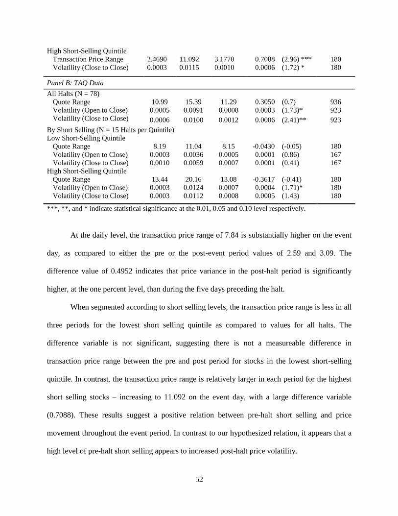
52
High Short-Selling Quintile
Transaction Price Range 2.4690 11.092 3.1770 0.7088 (2.96) *** 180
Volatility (Close to Close) 0.0003 0.0115 0.0010 0.0006 (1.72) * 180
Panel B: TAQ Data
All Halts (N = 78)
Quote Range 10.99 15.39 11.29 0.3050 (0.7) 936
Volatility (Open to Close) 0.0005 0.0091 0.0008 0.0003 (1.73)* 923
Volatility (Close to Close) 0.0006 0.0100 0.0012 0.0006 (2.41)** 923
By Short Selling (N = 15 Halts per Quintile)
Low Short-Selling Quintile
Quote Range 8.19 11.04 8.15 -0.0430 (-0.05) 180
Volatility (Open to Close) 0.0003 0.0036 0.0005 0.0001 (0.86) 167
Volatility (Close to Close) 0.0010 0.0059 0.0007 0.0001 (0.41) 167
High Short-Selling Quintile
Quote Range 13.44 20.16 13.08 -0.3617 (-0.41) 180
Volatility (Open to Close) 0.0003 0.0124 0.0007 0.0004 (1.71)* 180
Volatility (Close to Close) 0.0003 0.0112 0.0008 0.0005 (1.43) 180
***, **, and * indicate statistical significance at the 0.01, 0.05 and 0.10 level respectively.
At the daily level, the transaction price range of 7.84 is substantially higher on the event
day, as compared to either the pre or the post-event period values of 2.59 and 3.09. The
difference value of 0.4952 indicates that price variance in the post-halt period is significantly
higher, at the one percent level, than during the five days preceding the halt.
When segmented according to short selling levels, the transaction price range is less in all
three periods for the lowest short selling quintile as compared to values for all halts. The
difference variable is not significant, suggesting there is not a measureable difference in
transaction price range between the pre and post period for stocks in the lowest short-selling
quintile. In contrast, the transaction price range is relatively larger in each period for the highest
short selling stocks – increasing to 11.092 on the event day, with a large difference variable
(0.7088). These results suggest a positive relation between pre-halt short selling and price
movement throughout the event period. In contrast to our hypothesized relation, it appears that a
high level of pre-halt short selling appears to increased post-halt price volatility.

53
A similar pattern, for all halts and for both short selling categories, is identified with
close-to-close volatility: a sharp increase on the halt day and a reduction in the days following,
with post-halt values exceeding pre-halt values. The difference variable is statistically significant
for all firms and for high short-selling firms at the ten percent level; volatility appears mitigated
for stocks with low levels of short activity.
These results indicate that price variance for all sample firms increases substantially on
the halt day, then decrease considerably but remain elevated from pre-halt levels during the post-
halt period. This effect appears to be stronger for firms with higher levels of short selling,
suggesting that short selling activity translates into heightened price variability.
TAQ data is used to calculate daily quote ranges and open-to-close and close-to-close
volatility measurements (reported in Panel B). A substantial increase in the quote range (15.39)
is reported for all firms on the halt day; however, the pre and post halt quote range values are
similar in magnitude and the difference between them is not statistically different from zero. A
similar pattern is noted after segmenting halts according to short selling levels – high halt day
values, with quote ranges lower following the resumption of trading and insignificant differences
between the pre and post periods. However, the quote range during the event day for the highest
short selling stocks is nearly twice the quote range for the lowest quintile, and corresponding
quote range values are substantially higher during the pre and post halt periods.
Both volatility metrics demonstrate heightened levels on the event day, with open to close
volatility increasing by a factor of ten over both the pre and post halt periods. The difference
between the pre and post halt period is significant and positive. This result coincides with
Christie et al. (2002), who find that volatility increases to more than nine times normal levels for
NASDAQ halts that reopen after a five-minute quotation period.
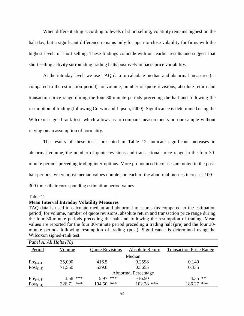
54
When differentiating according to levels of short selling, volatility remains highest on the
halt day, but a significant difference remains only for open-to-close volatility for firms with the
highest levels of short selling. These findings coincide with our earlier results and suggest that
short selling activity surrounding trading halts positively impacts price variability.
At the intraday level, we use TAQ data to calculate median and abnormal measures (as
compared to the estimation period) for volume, number of quote revisions, absolute return and
transaction price range during the four 30-minute periods preceding the halt and following the
resumption of trading (following Corwin and Lipson, 2000). Significance is determined using the
Wilcoxon signed-rank test, which allows us to compare measurements on our sample without
relying on an assumption of normality.
The results of these tests, presented in Table 12, indicate significant increases in
abnormal volume, the number of quote revisions and transactional price range in the four 30-
minute periods preceding trading interruptions. More pronounced increases are noted in the post-
halt periods, where most median values double and each of the abnormal metrics increases 100 –
300 times their corresponding estimation period values.
Table 12
Mean Interval Intraday Volatility Measures
TAQ data is used to calculate median and abnormal measures (as compared to the estimation
period) for volume, number of quote revisions, absolute return and transaction price range during
the four 30-minute periods preceding the halt and following the resumption of trading. Mean
values are reported for the four 30-minute period preceding a trading halt (pre) and the four 30-
minute periods following resumption of trading (post). Significance is determined using the
Wilcoxon signed-rank test.
Panel A: All Halts (78)
Period Volume Quote Revisions Absolute Return Transaction Price Range
Median
Pre(-4,-1) 35,000 416.5 0.2598 0.140
Post(1,4) 71,550 539.0 0.5655 0.335
Abnormal Percentage
Pre(-4,-1) 3.58 *** 5.97 *** -16.50 4.35 **
Post(1,4) 326.71 *** 104.50 *** 102.28 *** 186.27 ***
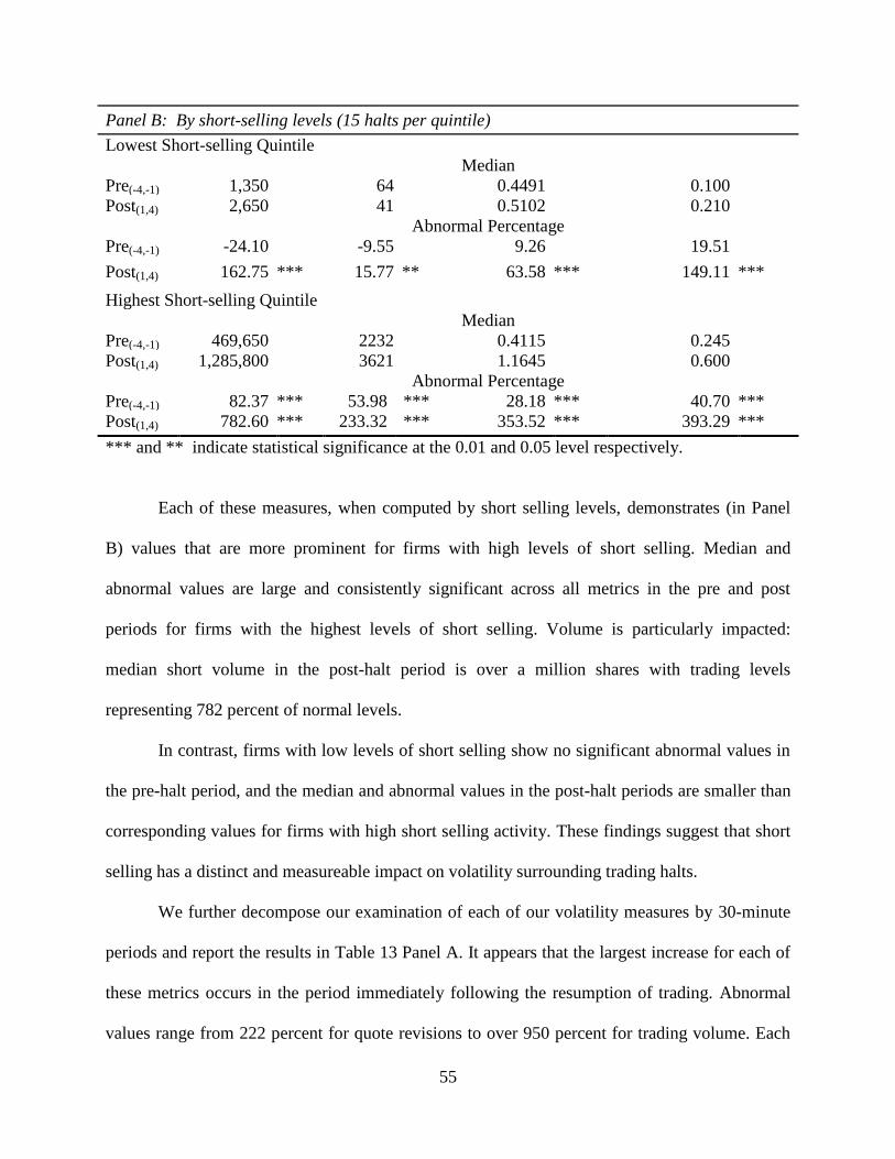
55
Panel B: By short-selling levels (15 halts per quintile)
Lowest Short-selling Quintile
Median
Pre(-4,-1) 1,350 64 0.4491 0.100
Post(1,4) 2,650 41 0.5102 0.210
Abnormal Percentage
Pre(-4,-1) -24.10 -9.55 9.26 19.51
Post(1,4) 162.75 *** 15.77 ** 63.58 *** 149.11 ***
Highest Short-selling Quintile
Median
Pre(-4,-1) 469,650 2232 0.4115 0.245
Post(1,4) 1,285,800 3621 1.1645 0.600
Abnormal Percentage
Pre(-4,-1) 82.37 *** 53.98 *** 28.18 *** 40.70 ***
Post(1,4) 782.60 *** 233.32 *** 353.52 *** 393.29 ***
*** and ** indicate statistical significance at the 0.01 and 0.05 level respectively.
Each of these measures, when computed by short selling levels, demonstrates (in Panel
B) values that are more prominent for firms with high levels of short selling. Median and
abnormal values are large and consistently significant across all metrics in the pre and post
periods for firms with the highest levels of short selling. Volume is particularly impacted:
median short volume in the post-halt period is over a million shares with trading levels
representing 782 percent of normal levels.
In contrast, firms with low levels of short selling show no significant abnormal values in
the pre-halt period, and the median and abnormal values in the post-halt periods are smaller than
corresponding values for firms with high short selling activity. These findings suggest that short
selling has a distinct and measureable impact on volatility surrounding trading halts.
We further decompose our examination of each of our volatility measures by 30-minute
periods and report the results in Table 13 Panel A. It appears that the largest increase for each of
these metrics occurs in the period immediately following the resumption of trading. Abnormal
values range from 222 percent for quote revisions to over 950 percent for trading volume. Each
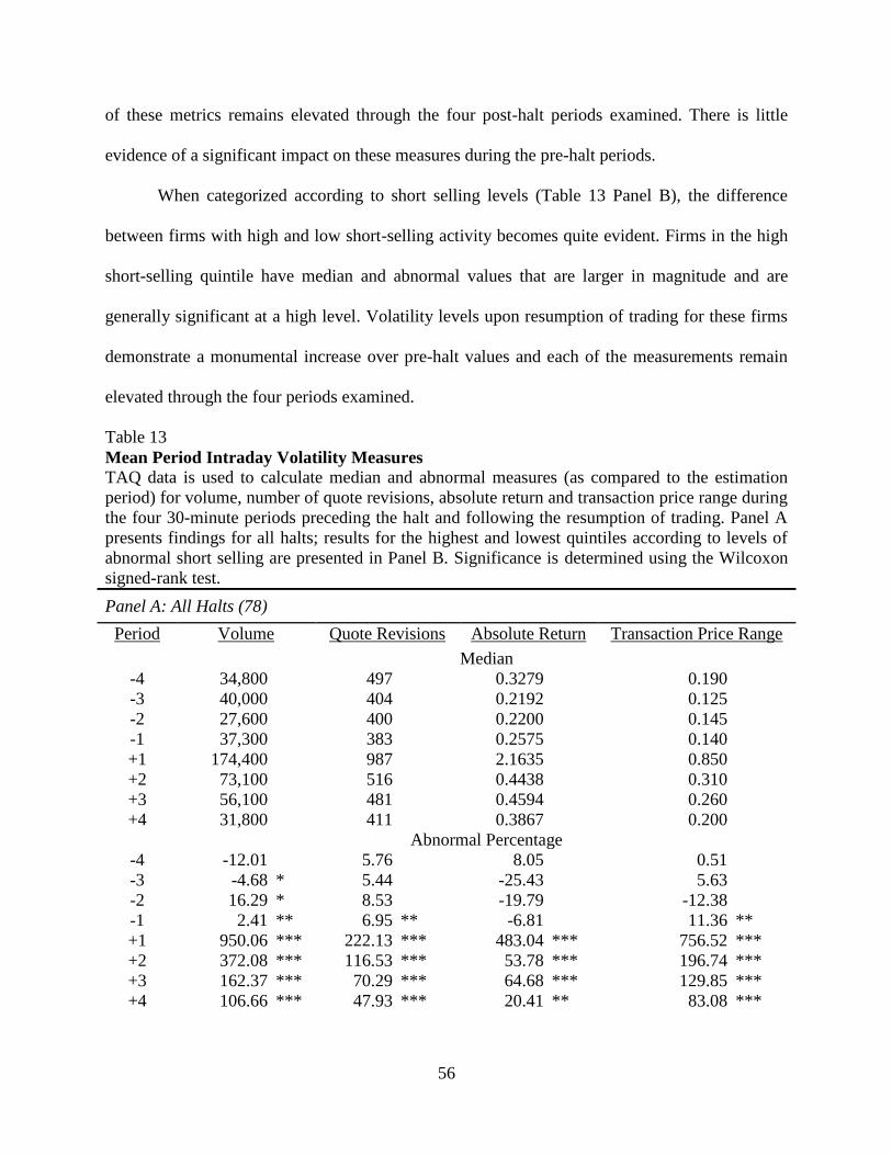
56
of these metrics remains elevated through the four post-halt periods examined. There is little
evidence of a significant impact on these measures during the pre-halt periods.
When categorized according to short selling levels (Table 13 Panel B), the difference
between firms with high and low short-selling activity becomes quite evident. Firms in the high
short-selling quintile have median and abnormal values that are larger in magnitude and are
generally significant at a high level. Volatility levels upon resumption of trading for these firms
demonstrate a monumental increase over pre-halt values and each of the measurements remain
elevated through the four periods examined.
Table 13
Mean Period Intraday Volatility Measures
TAQ data is used to calculate median and abnormal measures (as compared to the estimation
period) for volume, number of quote revisions, absolute return and transaction price range during
the four 30-minute periods preceding the halt and following the resumption of trading. Panel A
presents findings for all halts; results for the highest and lowest quintiles according to levels of
abnormal short selling are presented in Panel B. Significance is determined using the Wilcoxon
signed-rank test.
Panel A: All Halts (78)
Period Volume Quote Revisions Absolute Return Transaction Price Range
Median
-4 34,800 497 0.3279 0.190
-3 40,000 404 0.2192 0.125
-2 27,600 400 0.2200 0.145
-1 37,300 383 0.2575 0.140
+1 174,400 987 2.1635 0.850
+2 73,100 516 0.4438 0.310
+3 56,100 481 0.4594 0.260
+4 31,800 411 0.3867 0.200
Abnormal Percentage
-4 -12.01 5.76 8.05 0.51
-3 -4.68 * 5.44 -25.43 5.63
-2 16.29 * 8.53 -19.79 -12.38
-1 2.41 ** 6.95 ** -6.81 11.36 **
+1 950.06 *** 222.13 *** 483.04 *** 756.52 ***
+2 372.08 *** 116.53 *** 53.78 *** 196.74 ***
+3 162.37 *** 70.29 *** 64.68 *** 129.85 ***
+4 106.66 *** 47.93 *** 20.41 ** 83.08 ***
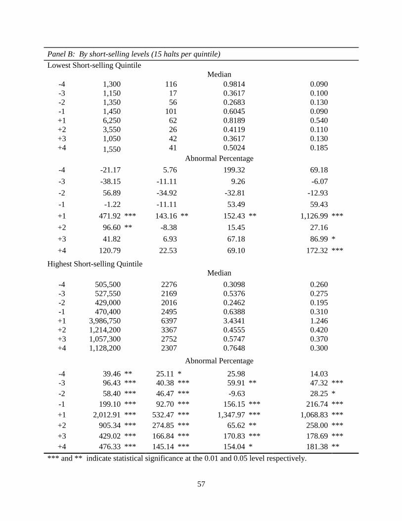
57
Panel B: By short-selling levels (15 halts per quintile)
Lowest Short-selling Quintile
Median
-4 1,300 116 0.9814 0.090
-3 1,150 17 0.3617 0.100
-2 1,350 56 0.2683 0.130
-1 1,450 101 0.6045 0.090
+1 6,250 62 0.8189 0.540
+2 3,550 26 0.4119 0.110
+3 1,050 42 0.3617 0.130
+4 1,550 41 0.5024 0.185
Abnormal Percentage
-4 -21.17 5.76 199.32 69.18
-3 -38.15 -11.11 9.26 -6.07
-2 56.89 -34.92 -32.81 -12.93
-1 -1.22 -11.11 53.49 59.43
+1 471.92 *** 143.16 ** 152.43 ** 1,126.99 ***
+2 96.60 ** -8.38 15.45 27.16
+3 41.82 6.93 67.18 86.99 *
+4 120.79 22.53 69.10 172.32 ***
Highest Short-selling Quintile
Median
-4 505,500 2276 0.3098 0.260
-3 527,550 2169 0.5376 0.275
-2 429,000 2016 0.2462 0.195
-1 470,400 2495 0.6388 0.310
+1 3,986,750 6397 3.4341 1.246
+2 1,214,200 3367 0.4555 0.420
+3 1,057,300 2752 0.5747 0.370
+4 1,128,200 2307 0.7648 0.300
Abnormal Percentage
-4 39.46 ** 25.11 * 25.98 14.03
-3 96.43 *** 40.38 *** 59.91 ** 47.32 ***
-2 58.40 *** 46.47 *** -9.63 28.25 *
-1 199.10 *** 92.70 *** 156.15 *** 216.74 ***
+1 2,012.91 *** 532.47 *** 1,347.97 *** 1,068.83 ***
+2 905.34 *** 274.85 *** 65.62 ** 258.00 ***
+3 429.02 *** 166.84 *** 170.83 *** 178.69 ***
+4 476.33 *** 145.14 *** 154.04 * 181.38 **
*** and ** indicate statistical significance at the 0.01 and 0.05 level respectively.
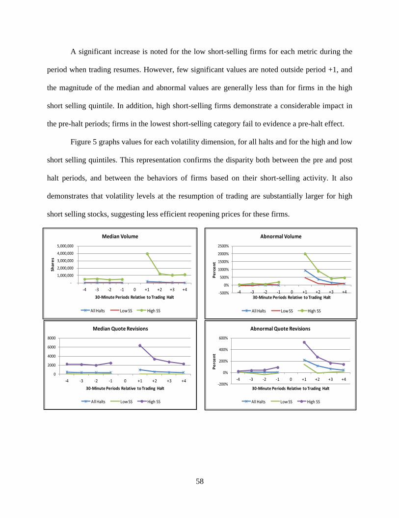
58
A significant increase is noted for the low short-selling firms for each metric during the
period when trading resumes. However, few significant values are noted outside period +1, and
the magnitude of the median and abnormal values are generally less than for firms in the high
short selling quintile. In addition, high short-selling firms demonstrate a considerable impact in
the pre-halt periods; firms in the lowest short-selling category fail to evidence a pre-halt effect.
Figure 5 graphs values for each volatility dimension, for all halts and for the high and low
short selling quintiles. This representation confirms the disparity both between the pre and post
halt periods, and between the behaviors of firms based on their short-selling activity. It also
demonstrates that volatility levels at the resumption of trading are substantially larger for high
short selling stocks, suggesting less efficient reopening prices for these firms.
-
1,000,000
2,000,000
3,000,000
4,000,000
5,000,000
-4 -3 -2 -1 0 +1 +2 +3 +4
Sh
are
s
30-Minute Periods Relative to Trading Halt
Median Volume
All Halts Low SS High SS
-500%
0%
500%
1000%
1500%
2000%
2500%
-4 -3 -2 -1 0 +1 +2 +3 +4
Pe
rce
nt
30-Minute Periods Relative to Trading Halt
Abnormal Volume
All Halts Low SS High SS
0
2000
4000
6000
8000
-4 -3 -2 -1 0 +1 +2 +3 +4
30-Minute Periods Relative to Trading Halt
Median Quote Revisions
All Halts Low SS High SS
-200%
0%
200%
400%
600%
-4 -3 -2 -1 0 +1 +2 +3 +4
Pe
rce
nt
30-Minute Periods Relative to Trading Halt
Abnormal Quote Revisions
All Halts Low SS High SS
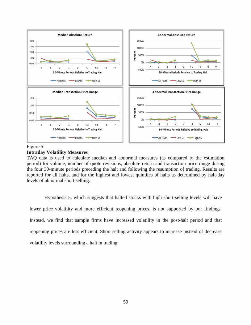
59
Figure 5
Intraday Volatility Measures
TAQ data is used to calculate median and abnormal measures (as compared to the estimation
period) for volume, number of quote revisions, absolute return and transaction price range during
the four 30-minute periods preceding the halt and following the resumption of trading. Results are
reported for all halts, and for the highest and lowest quintiles of halts as determined by halt-day
levels of abnormal short selling.
Hypothesis 5, which suggests that halted stocks with high short-selling levels will have
lower price volatility and more efficient reopening prices, is not supported by our findings.
Instead, we find that sample firms have increased volatility in the post-halt period and that
reopening prices are less efficient. Short selling activity appears to increase instead of decrease
volatility levels surrounding a halt in trading.
0.00
1.00
2.00
3.00
4.00
-4 -3 -2 -1 0 +1 +2 +3 +4
30-Minute Periods Relative to Trading Halt
Median Absolute Return
All Halts Low SS High SS
-500%
0%
500%
1000%
1500%
-4 -3 -2 -1 0 +1 +2 +3 +4
Pe
rce
nt
30-Minute Periods Relative to Trading Halt
Abnormal Absolute Return
All Halts Low SS High SS
0.00
0.50
1.00
1.50
-4 -3 -2 -1 0 +1 +2 +3 +4
30-Minute Periods Relative to Trading Halt
Median Transaction Price Range
All Halts Low SS High SS
-500%
0%
500%
1000%
1500%
-4 -3 -2 -1 0 +1 +2 +3 +4
Pe
rce
nt
30-Minute Periods Relative to Trading Halt
Abnormal Transaction Price Range
All Halts Low SS High SS
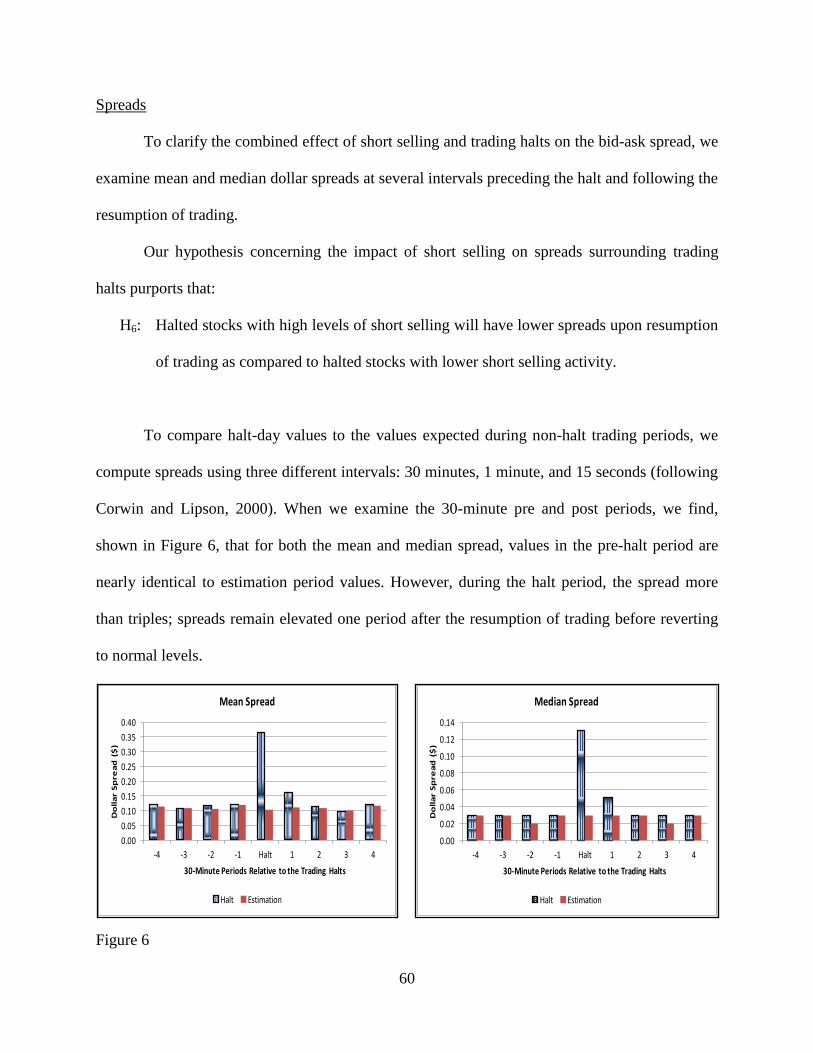
60
Spreads
To clarify the combined effect of short selling and trading halts on the bid-ask spread, we
examine mean and median dollar spreads at several intervals preceding the halt and following the
resumption of trading.
Our hypothesis concerning the impact of short selling on spreads surrounding trading
halts purports that:
H6: Halted stocks with high levels of short selling will have lower spreads upon resumption
of trading as compared to halted stocks with lower short selling activity.
To compare halt-day values to the values expected during non-halt trading periods, we
compute spreads using three different intervals: 30 minutes, 1 minute, and 15 seconds (following
Corwin and Lipson, 2000). When we examine the 30-minute pre and post periods, we find,
shown in Figure 6, that for both the mean and median spread, values in the pre-halt period are
nearly identical to estimation period values. However, during the halt period, the spread more
than triples; spreads remain elevated one period after the resumption of trading before reverting
to normal levels.
Figure 6
0.00
0.05
0.10
0.15
0.20
0.25
0.30
0.35
0.40
-4 -3 -2 -1 Halt 1 2 3 4
Do
lla
r S
pre
ad
($
)
30-Minute Periods Relative to the Trading Halts
Mean Spread
Halt Estimation
0.00
0.02
0.04
0.06
0.08
0.10
0.12
0.14
-4 -3 -2 -1 Halt 1 2 3 4
Do
lla
r S
pre
ad
($
)
30-Minute Periods Relative to the Trading Halts
Median Spread
Halt Estimation
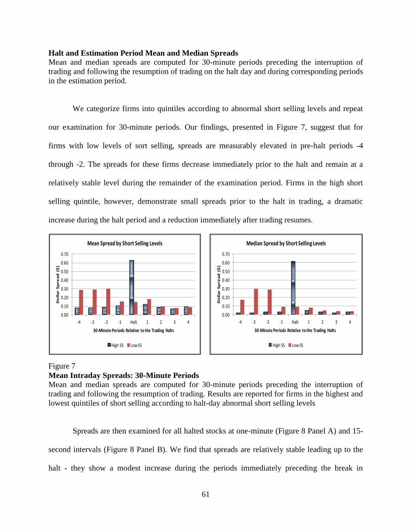
61
Halt and Estimation Period Mean and Median Spreads
Mean and median spreads are computed for 30-minute periods preceding the interruption of
trading and following the resumption of trading on the halt day and during corresponding periods
in the estimation period.
We categorize firms into quintiles according to abnormal short selling levels and repeat
our examination for 30-minute periods. Our findings, presented in Figure 7, suggest that for
firms with low levels of sort selling, spreads are measurably elevated in pre-halt periods -4
through -2. The spreads for these firms decrease immediately prior to the halt and remain at a
relatively stable level during the remainder of the examination period. Firms in the high short
selling quintile, however, demonstrate small spreads prior to the halt in trading, a dramatic
increase during the halt period and a reduction immediately after trading resumes.
Figure 7
Mean Intraday Spreads: 30-Minute Periods
Mean and median spreads are computed for 30-minute periods preceding the interruption of
trading and following the resumption of trading. Results are reported for firms in the highest and
lowest quintiles of short selling according to halt-day abnormal short selling levels
Spreads are then examined for all halted stocks at one-minute (Figure 8 Panel A) and 15-
second intervals (Figure 8 Panel B). We find that spreads are relatively stable leading up to the
halt - they show a modest increase during the periods immediately preceding the break in
0.00
0.10
0.20
0.30
0.40
0.50
0.60
0.70
-4 -3 -2 -1 Halt 1 2 3 4
Do
lla
r S
pre
ad
($
)
30-Minute Periods Relative to the Trading Halts
Mean Spread by Short Selling Levels
High SS Low SS
0.00
0.10
0.20
0.30
0.40
0.50
0.60
0.70
-4 -3 -2 -1 Halt 1 2 3 4
Do
lla
r S
pre
ad
($
)
30-Minute Periods Relative to the Trading Halts
Median Spread by Short Selling Levels
High SS Low SS
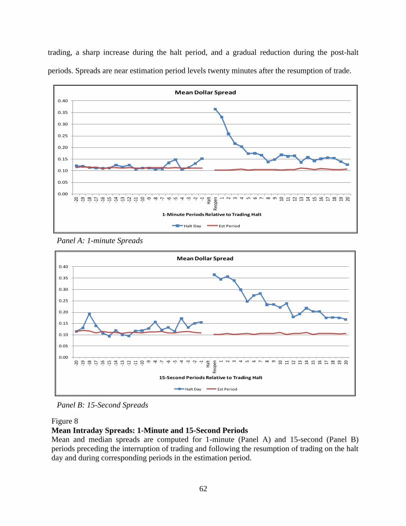
62
trading, a sharp increase during the halt period, and a gradual reduction during the post-halt
periods. Spreads are near estimation period levels twenty minutes after the resumption of trade.
Panel A: 1-minute Spreads
Panel B: 15-Second Spreads
Figure 8
Mean Intraday Spreads: 1-Minute and 15-Second Periods
Mean and median spreads are computed for 1-minute (Panel A) and 15-second (Panel B)
periods preceding the interruption of trading and following the resumption of trading on the halt
day and during corresponding periods in the estimation period.
0.00
0.05
0.10
0.15
0.20
0.25
0.30
0.35
0.40
-20
-19
-18
-17
-16
-15
-14
-13
-12
-11
-10 -9 -8 -7 -6 -5 -4 -3 -2 -1
Hal
tRe
open 1 2 3 4 5 6 7 8 9 10 11 12 13 14 15 16 17 18 19 20
1-Minute Periods Relative to Trading Halt
Mean Dollar Spread
Halt Day Est Period
0.00
0.05
0.10
0.15
0.20
0.25
0.30
0.35
0.40
-20
-19
-18
-17
-16
-15
-14
-13
-12
-11
-10 -9 -8 -7 -6 -5 -4 -3 -2 -1
Hal
t
Reop
en 1 2 3 4 5 6 7 8 9 10 11 12 13 14 15 16 17 18 19 20
15-Second Periods Relative to Trading Halt
Mean Dollar Spread
Halt Day Est Period
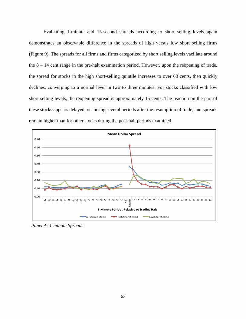
63
Evaluating 1-minute and 15-second spreads according to short selling levels again
demonstrates an observable difference in the spreads of high versus low short selling firms
(Figure 9). The spreads for all firms and firms categorized by short selling levels vacillate around
the 8 – 14 cent range in the pre-halt examination period. However, upon the reopening of trade,
the spread for stocks in the high short-selling quintile increases to over 60 cents, then quickly
declines, converging to a normal level in two to three minutes. For stocks classified with low
short selling levels, the reopening spread is approximately 15 cents. The reaction on the part of
these stocks appears delayed, occurring several periods after the resumption of trade, and spreads
remain higher than for other stocks during the post-halt periods examined.
Panel A: 1-minute Spreads
0.00
0.10
0.20
0.30
0.40
0.50
0.60
0.70
-20
-19
-18
-17
-16
-15
-14
-13
-12
-11
-10 -9 -8 -7 -6 -5 -4 -3 -2 -1
Hal
t
Reo
pen 1 2 3 4 5 6 7 8 9 10 11 12 13 14 15 16 17 18 19 20
1-Minute Periods Relative to Trading Halt
Mean Dollar Spread
All Sample Stocks High Short Selling Low Short Selling
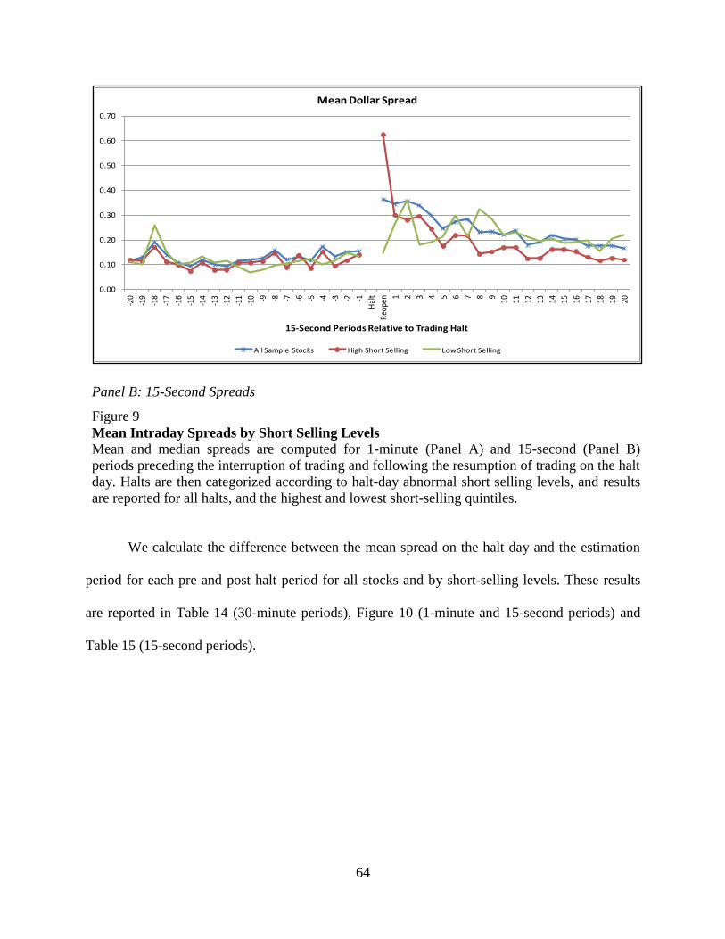
64
Panel B: 15-Second Spreads
Figure 9
Mean Intraday Spreads by Short Selling Levels
Mean and median spreads are computed for 1-minute (Panel A) and 15-second (Panel B)
periods preceding the interruption of trading and following the resumption of trading on the halt
day. Halts are then categorized according to halt-day abnormal short selling levels, and results
are reported for all halts, and the highest and lowest short-selling quintiles.
We calculate the difference between the mean spread on the halt day and the estimation
period for each pre and post halt period for all stocks and by short-selling levels. These results
are reported in Table 14 (30-minute periods), Figure 10 (1-minute and 15-second periods) and
Table 15 (15-second periods).
0.00
0.10
0.20
0.30
0.40
0.50
0.60
0.70
-20
-19
-18
-17
-16
-15
-14
-13
-12
-11
-10 -9 -8 -7 -6 -5 -4 -3 -2 -1
Hal
t
Reo
pen 1 2 3 4 5 6 7 8 9 10 11 12 13 14 15 16 17 18 19 20
15-Second Periods Relative to Trading Halt
Mean Dollar Spread
All Sample Stocks High Short Selling Low Short Selling
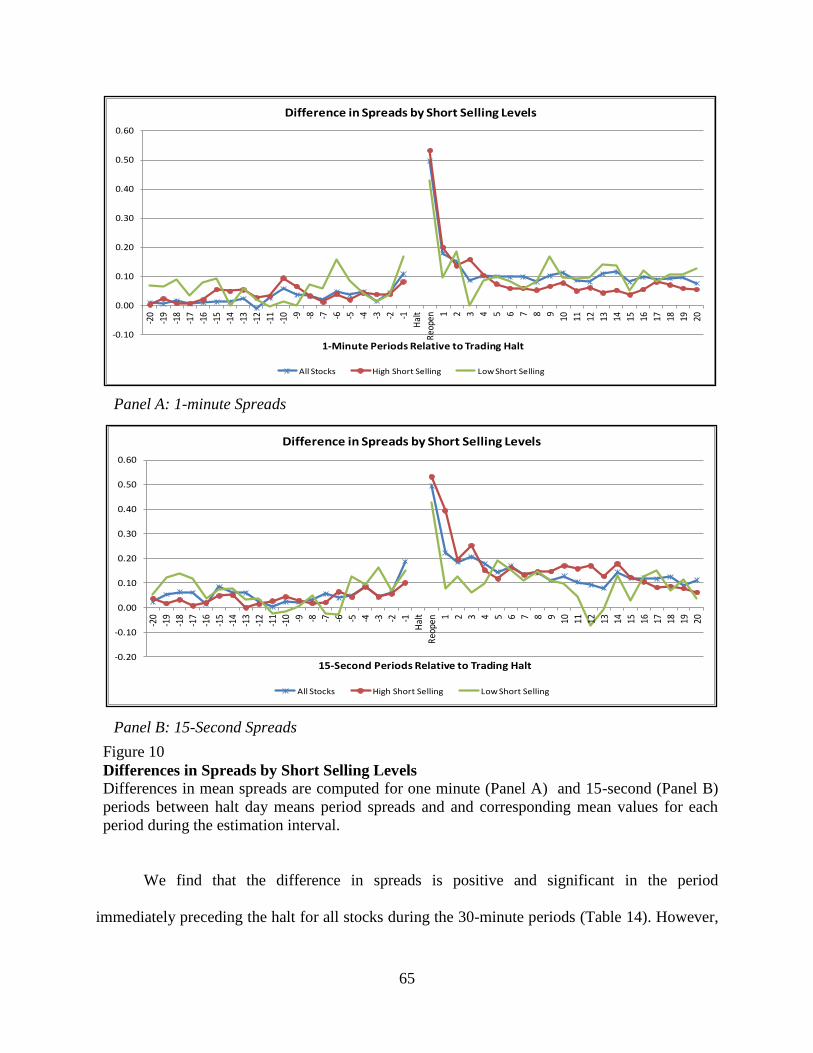
65
Panel A: 1-minute Spreads
Panel B: 15-Second Spreads
Figure 10
Differences in Spreads by Short Selling Levels
Differences in mean spreads are computed for one minute (Panel A) and 15-second (Panel B)
periods between halt day means period spreads and and corresponding mean values for each
period during the estimation interval.
We find that the difference in spreads is positive and significant in the period
immediately preceding the halt for all stocks during the 30-minute periods (Table 14). However,
-0.10
0.00
0.10
0.20
0.30
0.40
0.50
0.60
-20
-19
-18
-17
-16
-15
-14
-13
-12
-11
-10 -9 -8 -7 -6 -5 -4 -3 -2 -1
Hal
t
Reo
pen 1 2 3 4 5 6 7 8 9 10 11 12 13 14 15 16 17 18 19 20
1-Minute Periods Relative to Trading Halt
Difference in Spreads by Short Selling Levels
All Stocks High Short Selling Low Short Selling
-0.20
-0.10
0.00
0.10
0.20
0.30
0.40
0.50
0.60
-20
-19
-18
-17
-16
-15
-14
-13
-12
-11
-10 -9 -8 -7 -6 -5 -4 -3 -2 -1
Hal
t
Reo
pen 1 2 3 4 5 6 7 8 9 10 11 12 13 14 15 16 17 18 19 20
15-Second Periods Relative to Trading Halt
Difference in Spreads by Short Selling Levels
All Stocks High Short Selling Low Short Selling
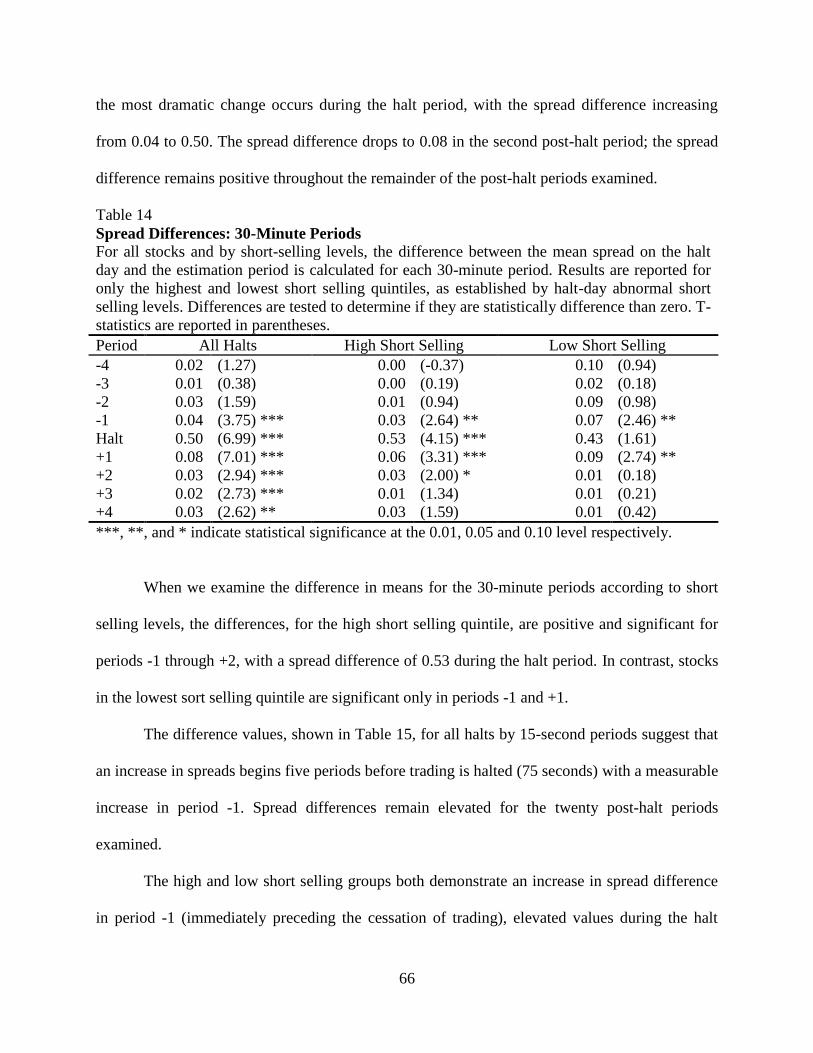
66
the most dramatic change occurs during the halt period, with the spread difference increasing
from 0.04 to 0.50. The spread difference drops to 0.08 in the second post-halt period; the spread
difference remains positive throughout the remainder of the post-halt periods examined.
Table 14
Spread Differences: 30-Minute Periods
For all stocks and by short-selling levels, the difference between the mean spread on the halt
day and the estimation period is calculated for each 30-minute period. Results are reported for
only the highest and lowest short selling quintiles, as established by halt-day abnormal short
selling levels. Differences are tested to determine if they are statistically difference than zero. T-
statistics are reported in parentheses.
Period All Halts High Short Selling Low Short Selling
-4 0.02 (1.27) 0.00 (-0.37) 0.10 (0.94)
-3 0.01 (0.38) 0.00 (0.19) 0.02 (0.18)
-2 0.03 (1.59) 0.01 (0.94) 0.09 (0.98)
-1 0.04 (3.75) *** 0.03 (2.64) ** 0.07 (2.46) **
Halt 0.50 (6.99) *** 0.53 (4.15) *** 0.43 (1.61)
+1 0.08 (7.01) *** 0.06 (3.31) *** 0.09 (2.74) **
+2 0.03 (2.94) *** 0.03 (2.00) * 0.01 (0.18)
+3 0.02 (2.73) *** 0.01 (1.34) 0.01 (0.21)
+4 0.03 (2.62) ** 0.03 (1.59) 0.01 (0.42)
***, **, and * indicate statistical significance at the 0.01, 0.05 and 0.10 level respectively.
When we examine the difference in means for the 30-minute periods according to short
selling levels, the differences, for the high short selling quintile, are positive and significant for
periods -1 through +2, with a spread difference of 0.53 during the halt period. In contrast, stocks
in the lowest sort selling quintile are significant only in periods -1 and +1.
The difference values, shown in Table 15, for all halts by 15-second periods suggest that
an increase in spreads begins five periods before trading is halted (75 seconds) with a measurable
increase in period -1. Spread differences remain elevated for the twenty post-halt periods
examined.
The high and low short selling groups both demonstrate an increase in spread difference
in period -1 (immediately preceding the cessation of trading), elevated values during the halt
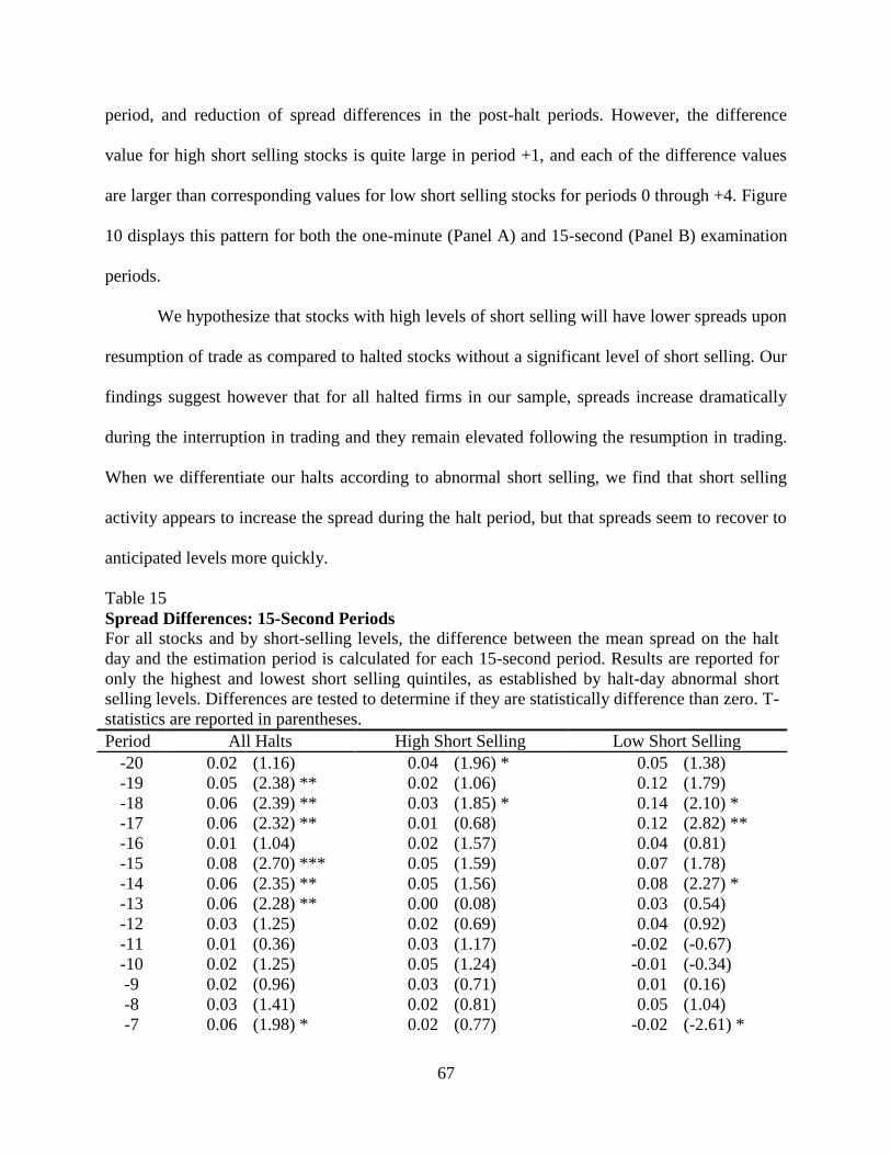
67
period, and reduction of spread differences in the post-halt periods. However, the difference
value for high short selling stocks is quite large in period +1, and each of the difference values
are larger than corresponding values for low short selling stocks for periods 0 through +4. Figure
10 displays this pattern for both the one-minute (Panel A) and 15-second (Panel B) examination
periods.
We hypothesize that stocks with high levels of short selling will have lower spreads upon
resumption of trade as compared to halted stocks without a significant level of short selling. Our
findings suggest however that for all halted firms in our sample, spreads increase dramatically
during the interruption in trading and they remain elevated following the resumption in trading.
When we differentiate our halts according to abnormal short selling, we find that short selling
activity appears to increase the spread during the halt period, but that spreads seem to recover to
anticipated levels more quickly.
Table 15
Spread Differences: 15-Second Periods
For all stocks and by short-selling levels, the difference between the mean spread on the halt
day and the estimation period is calculated for each 15-second period. Results are reported for
only the highest and lowest short selling quintiles, as established by halt-day abnormal short
selling levels. Differences are tested to determine if they are statistically difference than zero. T-
statistics are reported in parentheses.
Period All Halts High Short Selling Low Short Selling
-20 0.02 (1.16) 0.04 (1.96) * 0.05 (1.38)
-19 0.05 (2.38) ** 0.02 (1.06) 0.12 (1.79)
-18 0.06 (2.39) ** 0.03 (1.85) * 0.14 (2.10) *
-17 0.06 (2.32) ** 0.01 (0.68) 0.12 (2.82) **
-16 0.01 (1.04) 0.02 (1.57) 0.04 (0.81)
-15 0.08 (2.70) *** 0.05 (1.59) 0.07 (1.78)
-14 0.06 (2.35) ** 0.05 (1.56) 0.08 (2.27) *
-13 0.06 (2.28) ** 0.00 (0.08) 0.03 (0.54)
-12 0.03 (1.25) 0.02 (0.69) 0.04 (0.92)
-11 0.01 (0.36) 0.03 (1.17) -0.02 (-0.67)
-10 0.02 (1.25) 0.05 (1.24) -0.01 (-0.34)
-9 0.02 (0.96) 0.03 (0.71) 0.01 (0.16)
-8 0.03 (1.41) 0.02 (0.81) 0.05 (1.04)
-7 0.06 (1.98) * 0.02 (0.77) -0.02 (-2.61) *

68
-6 0.04 (1.49) 0.07 (1.84) * -0.03 (-0.54)
-5 0.05 (2.39) ** 0.04 (1.29) 0.13 (1.08)
-4 0.09 (2.49) ** 0.09 (1.7) 0.09 (1.60)
-3 0.05 (1.88) * 0.05 (1.41) 0.16 (2.40) *
-2 0.06 (1.76) * 0.06 (1.11) 0.07 (0.99)
-1 0.19 (3.54) *** 0.10 (2.10) * 0.15 (0.82)
Halt 0.50 (6.99) *** 0.53 (4.15) *** 0.43 (1.61)
1 0.22 (5.65) *** 0.40 (2.95) ** 0.08 (1.27)
2 0.19 (6.98) *** 0.20 (5.73) *** 0.13 (2.41) **
3 0.21 (8.09) *** 0.25 (6.25) *** 0.06 (2.84) **
4 0.18 (7.38) *** 0.15 (3.05) ** 0.10 (2.30) *
5 0.15 (5.25) *** 0.12 (3.81) *** 0.19 (1.86)
6 0.17 (7.37) *** 0.16 (5.50) *** 0.15 (3.39) **
7 0.13 (6.29) *** 0.13 (4.72) *** 0.11 (1.60)
8 0.14 (5.71) *** 0.15 (2.88) ** 0.15 (2.29) *
9 0.11 (5.15) *** 0.15 (2.46) ** 0.11 (2.53) **
10 0.13 (4.74) *** 0.17 (2.00) * 0.10 (1.58)
11 0.11 (4.48) *** 0.16 (2.58) ** 0.04 (1.05)
12 0.09 (3.56) *** 0.17 (2.25) ** -0.07 (-0.78)
13 0.08 (3.77) *** 0.13 (1.90) * -0.01 (-0.20)
14 0.15 (5.41) *** 0.18 (2.63) ** 0.13 (2.69) **
15 0.12 (5.57) *** 0.12 (2.72) ** 0.03 (0.46)
16 0.12 (5.87) *** 0.11 (3.45) *** 0.13 (1.60)
17 0.12 (4.20) *** 0.08 (3.19) *** 0.15 (1.86)
18 0.13 (5.81) *** 0.09 (3.37) *** 0.07 (1.00)
19 0.09 (4.28) *** 0.08 (2.50) ** 0.11 (1.98) *
20 0.11 (4.07) *** 0.06 (2.80) ** 0.03 (0.69)
***, **, and * indicate statistical significance at the 0.01, 0.05 and 0.10 level respectively.
69
CONCLUSION
Our research intent is to establish if short selling activity is altered surrounding trading
halts and determine if short sellers noticeably influence market quality and impact security prices
for halted firms. We hypothesize that short selling activity increases prior to a trading halt and
decreases following the resumption of trading. We further purport that halted firms with high
short selling activity, as compared to firms with lower levels of short selling, will experience a
larger price decline and a more rapid adjustment in price surrounding halts, and lower price
volatility and spreads after trading resumes.
We find little evidence at the daily level to support our proposition that short sellers
increase their activity prior to the implementation of a trading halt. We are unable to identify
increases in daily short trade size, number of trades or short volume prior to the event day.
However, our findings suggest that short sellers substantially modify their trading behavior
surrounding halts, as shorting metrics increase markedly on the halt day. An intraday
examination of shorting levels suggests a modest increase in activity in the two 30-minute
periods prior to the interruption in trading and a substantial increase in short selling in the
periods immediately following the reopening of trading. As anticipated, short selling values
decline in the post-halt period, but they remain elevated above estimation period levels during
the post-halt daily examination and for several periods following the resumption of trading on
the halt day itself.
Based on previous findings, our priori is that firms simultaneously undergoing a halt and
high levels of short selling will experience negative returns. However, at the daily level, when
70
categorized according to abnormal short selling levels, firms in the highest shorting category
demonstrate positive post-announcement returns. Chi-square test supports this conclusion by
demonstrating a shift of high short selling firms in the high return category; regression results
also indicate that pre-halt short selling increases for stocks with positive returns in the immediate
post-halt period.
At the intraday level, the highest and lowest short selling (ABSS) quintiles of firms
demonstrate positive returns during the trading interruption and negative returns immediately
following the reopening of trading. Short selling appears to amplify these returns, as values for
the high short-selling quintile are greater in magnitude. These findings suggest that relevant
information is primarily incorporated into prices after trading resumes and that short selling
assists the market in the price discovery process.
Results suggest that both trading halts and short selling activity affect the speed of price
adjustment. A comparison between halt day and estimation period speeds identify heightened
price movement in the period directly following the post-halt continuation of trading. Providing
support for Hypothesis 4, differentiating between the lowest and highest short selling stocks
indicates that the increase in the post-halt speed of price adjustment is more pronounced for
firms with higher shorting activity.
The majority of price contribution at the daily level occurs on the halt day, for all stocks
and for both the high and low short selling categories. At the intraday level, the weighted price
contribution for all halts occurs primarily during the halt and post-halt periods – very little
contribution is from the periods preceding the interruption in trading. However, for high short
selling firms, almost ninety percent of price impact occurs after the resumption of trading. In
71
contrast, the firms in the lowest short selling category demonstrate the highest price impact while
trading is halted.
When examining all firms, we find that intraday volatility measures fail to demonstrate a
substantial impact preceding the halt. However, volatility increases markedly following the
resumption of trading and it remains elevated through the post-halt periods examined. Short
selling activity, in contrast to our expected findings, appears to increase volatility surrounding
trading halts, as firms with high levels of short selling evidence both an impact prior to the
implementation of a halt and substantially larger values (as compared to firms with low levels of
short selling) in all periods.
Intraday spreads for all halts are relatively stable in the pre-halt periods, but they exhibit a
modest increase two periods before trading is interrupted. Spreads are highest during the halt
period and then gradually return to normal values. Upon the reopening of trading, the spreads for
stocks in the high short-selling category are substantially elevated, but return to expected values
within 20 minutes. For firms with the lowest short selling levels, reopening spreads do not show
as large of an increase, but they remain above normal values for the remainder of the periods
examined. Diether et al. (2009B) provides a rationale for the observed spread and volatility
behavior, stating that if short sellers act as opportunistic risk bearers during periods of
heightened uncertainty triggered by short-lived asymmetric information, then elevated levels of
short selling might occur in conjunction with high intraday volatility and wide spreads.
Although our empirical investigation yields findings that do not fully support our
proposed hypotheses, our results strongly indicate that short sellers modify their behavior
surrounding exchange-mandated halts in trading. The market quality of halted firms, in terms of

72
price, volatility and spreads, is impacted not only by the interruption in trading, but also by levels
of shorting activity.

73
LIST OF REFERENCES

74
Ackert, Lucy, Bryan Church, and Narayanan Jayaraman, 2001, An Experimental Study of
Circuit Breakers: The Effects of Mandated Market Closures and Temporary Halts on
Market Behavior, Journal of Financial Markets, 4, 185 – 208.
Aitken, Michael, Alex Frino, Michael McCorry, and Peter Swan, 1998, Short Sales are Almost
Always Bad News: Evidence from the Australian Stock Exchange, The Journal of
Finance, 53 (6), 2205 – 2223.
Angel, James, Stephen Christophe, and Michael Ferri, 2003, A Close Look at Short Selling on
Nasdaq, Financial Analyst Journal, 59 (6), 66 – 74.
Arnold, Tom, Alexander Butler, Timothy Crack and Yan Zhang, 2005, The Information Content
of Short Interest: A Natural Experiment, Journal of Business, 78 (4), 1307 – 1335.
Bacha, Obiyathulla, Eskandar Mohamed, and Roslily Ramlee, 2008, The Efficiency of Trading
Halts; Evidence from Bursa Malaysia, The International Journal of Banking and
Finance, 2 (5), 125 – 148.
Barclay, Michael, and Jerold Warner, 1993, Stealth Trading and Volatility, Journal of Financial
Economics, 34, 281 – 305.
Boehmer, Ekkehart, Charles Jones, and Xiaoyan Zhang, 2008, Which Shorts Are Informed?, The
Journal of Finance, 63 (2), 491 – 527.
Brent, A., D. Morse, and E.K. Stice, 1990, Short Interest: Explanations and Tests, Journal of
Financial and Quantitative Analysis, 25 (2), 273 – 289.
Bris, Arturo, 2008, Short Selling Activity in Financial Stocks and the SEC July 15th
Emergency
Order, IMD, Geneva, Obtained from website http://www.iimd.com/news/upload/
Chang, Eric, Joseph Cheng, and Yinghui Yu, 2007, Short-Sales Constraints and Price Discovery:
Evidence from the Hong Kong Market, The Journal of Finance, 62 (5), 2097 – 2122.
Christie, William, Shane Corwin, and Jeffrey Harris, 2002, Nasdaq Trading Halts: The Impact of
Market Mechanisms on Prices, Trading Activity, and Execution Costs, The Journal of
Finance, 57 (3), 1443 – 1478.
Christophe, Stephen, Michael Ferri, and James Angel, 2004, Short-Selling Prior to Earnings
Announcements, The Journal of Finance, 59 (4), 1845 – 1875.
Christophe, Stephen, Michael Ferri, and Jim Hsieh, 2010, Informed Trading Before Analyst
Downgrades: Evidence from Short Sellers, The Journal of Financial Economics, 95, 85 –
106.
Cohen, Lauren, Karl Diether, and Christopher Malloy, 2007, Supply and Demand Shifts in the
Shorting Market, The Journal of Finance, 62 (5), 2061 – 2096.
Copeland, Thomas, and Dan Galai, 1983, Information Effects on the Bid-Ask Spread, The
Journal of Finance, 38 (5), 1457 – 1469.

75
Corwin, Shane, and Marc Lipson, 2000, Order Flow and Liquidity around NYSE Trading Halts,
The Journal of Finance, 55 (4), 1771 – 1805.
Cox, Christopher, 2008, Public Statement by SEC Chairman: What the SEC Really Did on Short
Selling, July 24, “Op-Ed” for the Wall Street Journal, Obtained from website
http://www.sec.gov/news/speech/2008/spch072408cc.htm.
D’Avolio, 2002, The Market for Borrowing Stock, Journal of Financial Economics, 66, 271 –
306.
Dechow, Patricia, Amy Hutton, Lisa Meulbroek, and Richard Sloan, 2001, Short-sellers,
Fundamental Analysis, and Stock Returns, Journal of Financial Economics, 61, 77 – 106.
Desai, Hemang, K. Ramesh, S. Ramu Thiagarajan, and Bala Balachandran, 2002, An
Investigation of the Informational Role of Short Interest in the NASDAQ Market, The
Journal of Finance, 57 (5), 2263 – 2287.
Diamond, Douglas and Robert Verracchia, 1987, Constraints on Short-Selling and Asset Price
Adjustment to Private Information, Journal of Financial Economics, 18, 277 – 311.
Diether, Karl, Kuan-Hui Lee, and Ingrid Werner, 2009A, It’s SHO time! Short-Sale Price Tests
and Market Quality, The Journal of Finance, 64 (1), 37 – 73.
Diether, Karl, Kuan-Hui Lee, and Ingrid Werner, 2009B, Short-Sale Strategies and Return
Predictability, The Review of Financial Studies, 22 (2), 575 – 607.
Du, Yan, Qianqiu Liu, and S. Ghon Ree, 2005, An Anatomy of the Magnet Effect: Evidence
from the Korea Stock Exchange High Frequency Data, Working Paper, Obtained from
website: http://cei.ier.hit-u.ac.jp/activities/seminars/papers/Ghon%20Rhee.pdf
Easley, David, and Maureen O’Hara, 1987, Price, Trade Size, and Information in Securities
Markets, Journal of Financial Economics, 19, 69 – 90.
Engelen, Peter-Jan, and Rezaul Kabir, 2006, Empirical Evidence on the Role of Trading
Suspensions in Dissemination New Information to the Capital Market, Journal of
Business Finance & Accounting, 33 (7), 1142 – 1167.
Ferris, Stephen, Raman Kumar, and Glenn Wolfe, 1992, The Effect of SEC-Ordered
Suspensions on Returns, Volatility, and Trading Volume, The Financial Review, 27 (1), 1
– 34.
Geczy, Christopher, David Musto, and Adam Reed, 2002, Stocks are Special Too: An Analysis
of the Equity Lending Market, Journal of Financial Economics, 66, 241 – 269.
Goldstein, Michael, and Kenneth Kavajecz, 2004, Trading Strategies During Circuit Breakers
and Extreme Market Movements, Journal of Financial Markets, 7, 301 – 333.
Hasbrouck, Joel, 1991, Measuring the Information Content of Stock Trades, The Journal of
Finance, 46 (1), 179 – 207.

76
Hauser, Shmuel, Haim Kedar-Levy, Batia Pilo, and Itzhak Shurki, 2006, The Effect of Trading
Halts on the Speed of Price Discovery, Journal of Financial Services Research, 29 (1),
83 – 99.
Hopewell, Michael, and Arthur Schwartz Jr., 1978, Temporary Trading Suspensions in
Individual NYSE Securities, The Journal of Finance, 33 (5), 1355 – 1373.
Howe, John and Gary Schlarbaum, 1986, SEC Trading Suspensions: Empirical Evidence,
Journal of Financial and Quantitative Analysis, 21 (3), 323 – 333.
Jones, Charles, Gautam Kaul, and Marc Lipson, 1994, Transactions, Volume, and Volatility, The
Review of Financial Studies, 7 (4), 631 – 651.
Karpoff, Jonathan, 1986, A Theory of Trading Volume, The Journal of Finance, 41 (5), 1069 –
1087.
Karpoff, Jonathan, 1987, The Relation Between Price Changes and Trading Volume: A Survey,
Journal of Financial and Quantitative Analysis, 22 (1), 109 – 126.
Karpoff, Jonathan, and Xiaoxia Lou, 2010, Short Sellers and Financial Misconduct, The Journal
of Finance, 65 (5), 1879 – 1913.
Kim, Yong, José Yague, and J. Jimmy Yang, 2008, Relative Performance of Trading Halts and
Price Limits: Evidence from the Spanish Stock Exchange, International Review of
Economics & Finance, 17 (2), 197 – 215.
Kim, Kenneth, and S. Ghon Rhee, 1997, Price Limit Performance: Evidence from the Tokyo
Stock Exchange, The Journal of Finance, 52 (2), 885 – 901.
Kim, Yong, and J. Jimmy Yang, 2004, What Makes Circuit Breakers Attractive to Financial
Markets? A Survey, Financial Markets, Institutions & Instruments, 13 (3), 109 – 146.
Koski, Jennifer, and Roni Michaely, 2000, Prices, Liquidity, and the Information Content of
Trades, The Review of Financial Studies, 13 (3), 659 – 696.
Kryzanowski, Lawrence, 1979, The Efficacy of Trading Suspensions: A Regulatory Action
Designed to Prevent the Exploitation of Monopoly Information, The Journal of Finance,
34 (5), 1187 – 1200.
Kryzanowski, Lawrence and Howard Nemiroff, 1998, Price Discovery Around Trading Halts on
the Montreal Exchange Using Trade-by-Trade Data, The Financial Review, 33, 195 –
212.
Kryzanowski, Lawrence, and Howard Nemiroff, 2001, Market Quote and Spread Component
Cost Behavior Around Trading Halts for Stocks Interlisted on the Montreal and Toronto
Stock Exchanges, The Financial Review, 37, 115 – 138.
Kyle, Albert, 1985, Continuous Auctions and Insider Trading, Econometrica, 53 (6), 1315 –
1335.

77
Lee, Charles, J. Ready, and Paul Seguin, 1994, Volume, Volatility, and New York Stock
Exchange Trading Halts, The Journal of Finance, 49 (1), 183 – 214.
Madura, Jeff, Nivine Richie, and Alan Tucker, 2006, Trading Halts and Price Discovery, Journal
of Financial Services Research, 30, 311 – 328.
McInish, Thomas, and Robert Wood, 1991, Hourly Returns, Volume, Trade Size, and Number of
Trades, The Journal of Financial Research, 14 (4), 303 – 315.
Miller, Edward, 1977, Uncertainty, and Divergence of Opinion, The Journal of Finance, 32 (4),
1151 – 1168.
Reed, Adam, 2007, Costly Short Selling and Stock Price Adjustments to Earnings
Announcements, Working Paper, Obtained from website:
http://www.nd.edu/~carecob/April%202007%20Conference/Costly%20Short%20Selling
%20and%20Stock%20Price%20Adjustment%20to%20Earnings%20Announcements.pdf
Rooney, Ben, 2010, SEC Moves to Expand Stock Circuit Breakers, May 18. CNNMoney.com,
Obtained from website http://money.cnn.com/2010/05/18/markets/SEC_circuit_breakers/.
Safieddine, Assem, and William Wilhelm Jr., 1996, An Empirical Investigation of Short-Selling
Activity Prior to Seasoned Equity Offerings, The Journal of Finance, 51 (2), 729 – 749.
Senchack, A. J., and Laura Starks, 1993, Short-Sale Restirictions and Market Reaction to Short-
Interest Announcements, Journal of Financial and Quantitative Analysis, 28 (2), 177 –
194.
Seppi, Duane, 1990, Equilibrium Block Trading and Asymmetric Information, The Journal of
Finance, 45 (1), 73 – 94.
Spiegel, Matthew, and Avanidhar Subrahmanyam, 2000, Asymmetric Information and News
Disclosure Rules, Journal of Financial Intermediation, 9, 363 – 403.
Subrahmanyam, Avanidhar, 1994, Circuit Breakers and Market Volatility: A Theoretical
Perspective, The Journal of Finance, 49 (1), 237 – 254.
The Wall Street Journal. May 18, 2010. SEC Statement on Proposed Circuit Breakers. Retrieved
from website http://blogs.wsj.com/dispatch/2010/05/18/sec-seeks-comment-on-proposed-
circuit-breakers/?KEYWORDS=Mary+Schapiro+circuit+breakers.
Westerhoff, Frank, 2003, Speculative Markets and the Effectiveness of Price Limits, Journal of
Economic Dynamics and Control, 28, 493 – 508.
Wong, Woon, Matthew Chang, and Anthony Tu, 2009, Are Magnet Effects caused by
Uniformed Traders? Evidence from the Taiwan Stock Exchange, Pacific-Basin Finance
Journal, 17, 28 – 40.
Wu, Ho-Mou and Wen-Chung Guo, 2004, Asset Price Volatility and Trading Volume with
Rational Beliefs, Economic Theory, 23, 795 – 829.
78
ESSAY 2:
CONTAGIOUS SHORT SELLING SURROUNDING TRADING HALTS
79
INTRODUCTION
The purpose of this paper is to determine if a short-selling contagion effect exists for
contemporaries of firms experiencing a trading halt. Although trading suspensions represent a
firm-specific event, they may be viewed as ‘contagious’ in the sense that they contain
information relevant to other firms in the same industry. Recent studies demonstrate the presence
of a contagion effect surrounding trading halts and they describe the associated impact on the
market quality of related firms.6 However, research does not establish whether interruptions in
trading affect short selling activity for industry contemporaries. Our examination addresses this
research issue; the potential for an intra-industry effect prompts us to examine if shorting levels
vary significantly for organizations that are informationally related to a firm experiencing a
trading halt. We also measure the impact of short sales on the market quality of these
contemporary firms by examining their returns, price volatility, and spreads surrounding
interruptions in trading for an industry member.
TRADING HALTS
Financial markets have regulations that suspend trading under specified conditions. These
interruptions in trading can take the form of price limits, which are implemented when security
prices cross boundaries established by market regulators, firm-specific trading halts that suspend
trading on an individual security for a predetermined period, or market-wide circuit breakers that
halt trading on the entire market when a designated index exceeds a pre-specified level. Firm-
6 Refer to Spiegel and Subrahmanyam (2000); and Jiang, McInish, and Upson (2009)

80
specific trading halts can be further categorized according to their underlying cause; halts can be
either news-related or they can be prompted by an order imbalance. A news-related trading halt
is triggered by exchange officials when an information release is expected to have or
demonstrates a significant impact on security prices. In contrast, an order imbalance trading halt
is instigated when an exchange specialist observes a large imbalance between buy and sell orders
(Kim and Yang 2004).
LITERATURE REVIEW
Research describes the impact of informational events on the affected firm. Previous
researchers establish the presence of financial contagion and commonality in order flow for firms
in the same industry and they demonstrate the impact, in terms of market quality and short
selling activity, of an informational event on related firms. Our literature review describes this
body of research and discusses how it pertains to our examination of short selling activity for
informationally related firms surrounding interruptions in trading.
The Impact of Informational Events on the Affected Firm
Market Quality
A significant price, volatility, and liquidity impact on the securities of firms experiencing
an informational event, such as earnings announcements, dividend declarations, bankruptcy
announcements, stock splits, and trading halts, is demonstrated by prior research. These findings
provide an important contribution to our current study; namely, that corporate events contain
81
information and subsequently they have a measurable impact on the market quality of the
affected firm.7
In addition, this body of research provides evidence that informed market participants
play a crucial role in the dynamic trading environment surrounding informational events. For
instance, Bajaj and Vijh (1995) purport that excess returns surrounding dividend announcements
represents compensation for the risk accepted by informationally motivated traders. Desai,
Nimalendran, and Venkataraman (1998) report increases in volatility and spreads surrounding
National Association of Securities Dealers Automated Quotations (NASDAQ) stock splits; their
findings suggest that changes in trading activity are due, in part, to the actions of informed
traders.
Short Selling
Microstructure literature shows that short sellers are informed traders that have the ability
to earn abnormal returns in environments with elevated levels of information asymmetry.8 This
research stream also demonstrates that short selling increases prior to informational events –
suggesting that short sellers possess important private information prior to its public revelation.9
Two examinations of short selling behavior preceding informational events hold
particular importance for our investigation of firm-specific trading halts. In the first, Aitken,
Frino, McCorry, and Swan (1998), suggest a higher probability of informed trading for short
7 Beaver (1968); Lee, Mucklow, and Ready (1993); Aharony and Swary (1980); Datta and Iskandar-Datta (1995);
Dawkins, Bhattacharya, and Bamber (2007); Lamoureux and Poon (1987); Conroy, Harris, and Benet (1990);
Madura, Richie, and Tucker (2006); Kryzanowski (1979); Howe and Schlarbaum (1986); Ferris, Kumar, and Wolfe
(1992); Christie, Corwin and Harris (2002); Corwin and Lipson (2000); Lee, Ready, and Senguin (1994); Bacha,
Mohamed, and Ramlee (2008); Engelen and Kabir (2006); Hauser, Kedar-Levy, Pilo, and Shurki. (2006); Kim and
Rhee (1997); and Kryzanowski and Nemiroff (1998), provide specific examples. 8 Specific examples are provided by Senchack and Starks (1993); Arnold, Butler, Crack , and Zhang (2005); Chang,
Cheng, and Yu (2007); Boehmer, Jones, and Zhang (2008); and Diether, Lee, and Werner (2009B). 9 Refer to Safieddine and Wilhelm (1996); Karpoff and Lou (2010); Blau, Fuller, and Van Ness. (2011); and
Christophe, Ferri, and Hsieh (2010).
82
transactions that execute the day prior to a trading halt. In the second, Christophe, Ferri, and
Angel (2004) demonstrate that short selling activity preceding earnings announcements reflects
firm-specific information.
The above-mentioned literature purports that certain firm-specific events provide a source
of information for the market. It establishes that these events are associated with a measureable
impact on the market quality of the corporation experiencing the event and it demonstrates that
short sellers, who are deemed informed market participants, appear to recognize the potential
information content of the announcements and to their advantage, successfully anticipate the
market’s reaction.
Financial Contagion and Commonality
Financial contagion, in a broad interpretation, refers to increases in volatility and the
comovement of financial asset markets between countries (Kodres and Pritsker 2002),
particularly following an economic shock to one country. Our research relies on a more narrow
definition of contagion, one that refers to this same comovement and increase in volatility, but
restricts itself to firms in the same or related industries surrounding an informational event for
one company. Supporting this view, Kaufman (1994, page 123) describes contagion as “… the
spillover of the effects of shocks from one or more firms to others,” Alli, Thapa, and Yung
(1994, page 1059) as “the transmission mechanism of stock price formation of industrial firms
within a particular national market,” and Ghosh, Guttery, and Sirmans (1998, page 592) as the
market’s use, “… of information about one firm’s poor performance to infer that similar
problems exist with other firms …”
83
Research into industry contagion establishes the commonality of returns, order flow, and
transaction costs between related firms. For instance, Chordia, Roll, and Subrahmanyam (2000)
find that the components of liquidity for a firm are closely associated with market and industry
liquidity. Similarly, Huberman and Halka (2001) demonstrate the existence of a systematic
component of liquidity. In their examination of Dow Jones Stocks, Hasbrouck and Seppi (2001)
find the presence of common factors in both order flow and returns. Subrahmanyam (1991, page
44) examines market liquidity and price informativeness for baskets of securities. His research
implies the, “strong tendency for both movements in the price of the basket and movements in
the price of the portfolio to provide predictive information about subsequent price movements in
the other.”
Contagion is examined extensively in the banking and finance industry. For example,
Lang and Stulz (1992) examine the impact of bankruptcy announcements on the value of firms
operating within an industry and find support for the presence of industry contagion. However,
their research also identifies the presence of a competitive effect – a gain in wealth by the rivals
of the firm announcing bankruptcy. This gain is attributed to the information conveyed through
the announcement regarding the potential redistribution of wealth from the bankrupt firm to its
competitors and the anticipated improved competitive posture of other industry firms.
Ferris, Jayaraman, and Makhja (1997) extend Lang and Stulz’s research and attempt to
identify which related firms will experience a contagion or competitive effect. In line with Lang
and Stulz, they find that bankruptcy announcements generate contagion. They further purport
that the inability of their research to detect a competitive effect might be attributed to the fact
that prior to Chapter 11 filing, the impact of the bankruptcy announcement is already
incorporated into the stock prices of related firms. This notion suggests the presence of informed
84
trading – select investors are able to predict accurately both the impending bankruptcy and its
impact, either positive or negative, on informationally related firms.
Bessler and Nohel (2000) examine bank stock returns surrounding dividend
announcements to test for the presence of a contagion effect in environments with high levels of
information asymmetry (bank insiders hold extensive amounts of confidential information). They
find that dividend reductions induce negative abnormal returns for non-announcing banks.
Additionally, they find that these contagion effects seem to be consistent with informed trading –
the presence of contagion is related to firm characteristics that are common amongst affected
institutions.
The results of Ferris et al. and Bessler and Nohel emphasize the import role that informed
market participants play surrounding firm-specific informational events. Their findings regarding
contagious informed trading, particularly in environments with high information asymmetry,
provide support for our inquiry into potential changes in the levels of short selling for the
industry competitors of halted firms.
The Impact of Informational Events on the Related Firm
Market Quality
Solidifying the relation between industry contemporaries, Tookes (2008) examines
earnings announcements, and develops a model of informed trading that demonstrates how
informational events can affect multiple firms in the same industry. This model predicts that it is
advantageous for informed traders to execute information-based trades in securities for
competitors and it demonstrates that competitors’ trading levels and returns contain information
beyond that of the order flow and returns of the firm experiencing an informational event.

85
Spiegel and Subrahmanyam (2000) demonstrate that a contagion or commonality effect
occurs surrounding interruptions in trading. They construct a multi-security model that describes
how a trading halt for a security can decrease liquidity and increase price volatility for stocks in
the same industry. They purport that trading halts signal a state of information asymmetry for
informationally related firms.
Building upon Spiegel and Subrahmanyam’s research and Tookes’ model of informed
trading, Jiang, McInish, and Upson (2009, page 704) examine the relation between financial
contagion and interruptions in trading. They state, “Under the Tookes model, an informational
event in one stock in an industry can instigate informed and insider trading in related stocks in
that industry …” Jiang et al. offer evidence of contagion by demonstrating the impact of New
York Stock Exchange (NYSE) trading halts, including increases in spreads, price impact, and
trading volume, on firms that are informationally related.
Short Selling
Previous research purports that short sellers are informed market participants. Building
upon this notion, a theoretical justification for an increase in short selling for related firms
surrounding an informational event is provided by Tookes (2008). She suggests that when the
informed insiders of a halted firm are restricted from shorting their own stocks, they or their
proxies take advantage of their superior industry knowledge and submit informed trades on
informationally related securities (Jiang et al. 2009).
Providing empirical support for Tookes’ proposition, Efendi, Kinney, and Swanson
(2005) examine changes in short selling levels for corporations that announce they will restate
financial statements due to accounting irregularities. These researchers find evidence of a

86
contagion effect – increases in levels of short interest for corresponding industry firms. Further,
they purport that short sellers have superior knowledge; the majority of short-selling increases
were for firms related to companies restating major irregularities. This research supports the
notion that short sellers are informed and provides an essential link between informational events
and short selling for related firms.
Our investigation differs from the work of Efendi et al. (2005) in two significant ways.
First, their examination demonstrates increases in short interest for industry and size matched
counterpart firms after the announcement of a restatement. We purport that short seller expertise
will allow short sellers to increase their activity prior to the implementation of a trading halt; we
anticipate heightened short selling preceding an informational trading halt event. Second, Effendi
et al. focus on how short sellers utilize accounting information to identify over-valued firms,
whereas our investigation relies on short sellers responding to short-term changes in market
activity.
We rely on the Tookes’ model and the findings of Efendi et al. (2005) to hypothesize that
short sellers will increase their trading activity for industry contemporaries surrounding
interruptions in trading. Further, we extend the demonstrated relation between firm specific
trading halts and a market response for informationally related firms provided by Jiang et al.
(2009), and Spiegel and Subrahmanyam (2000), to examine whether changes in short selling
activity for related firms substantially alter their market quality.
87
HYPOTHESES
Existing literature demonstrates that informational events have a significant impact on the
market quality of affected firms and that short selling for these firms increases prior to firm-
specific informational events. It also establishes that a contagious reaction, consisting of changes
in market quality and increases in short selling, occurs for industry contemporaries surrounding
an informational event. These findings provide a cornerstone for our assertion that an
informational event for one firm can significantly influence related firms. We extend this
research to determine if this contagion effect includes short selling activity surrounding
interruptions in trading.
Short Selling
Market microstructure literature establishes that short sellers possess superior private
information. It also demonstrates the presence of intra-industry contagion surrounding
informational events, including trading halts, and it demonstrates that short selling increases
prior to informational events for both affected and informationally related firms. We build upon
these findings and suggest that industry contemporaries of a firm subject to a trading halt will
experience increases in short-selling activity. To document short seller behavior, we examine
several trading metrics that quantify the level of short sales for these related firms:
88
H1: Surrounding a trading halt, securities that are informationally related to a halted stock
will experience a significant increase in the number of short transactions, short interest
ratio, relative short selling, and abnormal short selling measures.
Market Quality - Returns, Price Volatility and Spreads
Interruptions in trading have a significant effect on the market quality of halted firms.
Madura et al. (2006), provide an overview of the literature’s findings regarding the impact of
trading halts on returns, price volatility, and spreads. They summarize, stating that in general,
stocks undergoing a trading halt: (1) experience abnormal negative returns, and (2) following a
trading halt, volatility is elevated and spreads remain wide. Jiang et al. (2009, page 705) state, “a
firm-specific trading halt is an informational event that impacts the market beyond that of the
halted company.” In the presence of contagion and commonality of returns, order flow, and
transaction costs, it follows that informationally related firms will experience similar changes in
their market quality.
Returns
Securities with high short-selling levels typically experience price declines. Providing
empirical support for this assertion, Senchack and Starks (1993), Desai, Ramesh, and
Thiagarajan (2002), and Cohen, Diether, and Malloy (2007) demonstrate that increases in short
interest generate negative abnormal returns. Boehmer et al. (2008) find that heavily shorted
stocks underperform annually by a risk-adjusted 15.6 percent as compared to lightly shorted
stocks, and Diether et al. (2009B) find that during periods of high asymmetric information, short
sale transactions are followed by negative returns.
89
Providing support for the asserted negative relation between trading halts and returns,
Kryzanowski (1979) finds significant abnormal negative returns surrounding halts in trading, and
Howe and Schlarbaum (1986) report that almost 80 percent of halted securities experience
negative abnormal returns during the suspension period.
Demonstrating the impact of informational events on related firms, Lang and Stulz
(1992) examine the impact of bankruptcy announcements and find that the market value of a
portfolio containing the common stock of a bankrupt firm’s competitors experiences a
considerable decrease following a firm’s bankruptcy announcement. Bessler and Nohel (2000)
examine bank stock returns surrounding dividend announcements and find that dividend
reductions induce negative abnormal returns for non-announcing banks. In addition, Jiang et al.
(2009) find, consistent with the informed trading model of Tookes, an increase in the price
impact of trades for informationally related firms during halts in trading.
Based on the findings of negative abnormal returns surrounding both trading halts and
high short selling levels, and the increased impact of trades for related firms surrounding
informational events, specifically trading halts, we purport that firms with higher levels of short
selling will experience a larger price decline:
H2: Securities that are informationally related to a halted stock and have high short selling
levels will experience a larger decline in price surrounding a trading halt as compared
to informationally related stocks with lower short selling activity.
90
Price Volatility
Chang et al. (2007) examine the relation between short selling and volatility and find that
when short selling is permitted, the volatility of both raw and abnormal returns increases
substantially. Likewise, Wu and Guo (2004) and Angel, Christophe, and Ferri (2003) find that
short selling levels are directly related to price volatility.
The findings of Kim and Rhee (1997), Kryzanowski and Nemiroff (1998), and Ferris et
al. (1992) provide support for the notion that stock volatility is not mitigated by interruptions in
trading. Similarly, Christie et al. (2002) find elevated volatility following NASDAQ trading
halts, and Lee et al. (1994), who investigate firm-specific NYSE trading halts, find that post-halt
volatility levels are elevated 50 to 115 percent. We purport that surrounding interruptions in
trading, informationally related stocks experience a similar increase in volatility as halted stocks.
Spiegel and Subrahmanyam (2000, page 388) state, “… high volatility of price changes in one
stock should be followed by a high volatility in another stock with a positively correlated private
information variance (e.g. another stock in the same industry).”
Considering the increase in volatility described by both the trading halt and the short
selling literature and the anticipated contagion of volatility from halted stocks to industry
contemporaries, we predict that informationally related stocks with increased short selling
activity will experience higher volatility levels:
H3: Securities that are informationally related to a halted stock and have high short selling
levels will have higher price volatility surrounding trading halts as compared to
informationally related securities with lower levels of short selling activity.

91
Spreads
The bid-ask spread is used by dealers to balance the gains they receive from liquidity
traders with losses suffered to informed traders who are better able to forecast future prices
(Copeland and Galai 1983). If large transactions are viewed as having higher information
content, as purported by Easley and O’Hara (1987), they should cause the spread to widen to
provide compensation to dealers for their informational disadvantage (Hasbrouck 1991). If
informed short-sellers submit large transaction in an attempt to increase the price impact of their
trades, we would expect to see a positive relation between short selling levels and spreads.
Diether, Lee, and Werner (2009A) find support for this notion; they examine pilot stocks, for
which short-selling tests are suspended, and find that increases in short selling activity lead to
increases in quoted and effective spreads.
Spiegel and Subrahmanyam (2000) suggest that during the trading suspension, the ask
(bid) price of an informationally related security will be greater (less) than during a non-halt
period. They explain that liquidity traders withdraw from the market after observing high levels
of information asymmetry. Subsequently, the market maker observes both the increased
asymmetry and the decrease in liquidity and widens spreads to compensate for losses to informed
traders. Providing empirical support for this belief, Jiang et al. (2009) find that firm-specific
trading halts increase spreads significantly for informationally related firms.
Spreads widen surrounding trading halts and with increases with short selling activity. It
follows then, that a firm that is both informationally related to a halted firm and experiences high
levels of shorting will evidence wider spreads:
92
H4: Securities that are informationally related to a halted stock and have high short selling
levels will have wider spreads surrounding trading halts as compared to informationally
related securities with lower levels of short selling activity.
DATA
We first identify NYSE and American Stock Exchange (AMEX) trading halts that occur
during 2005–2006 by querying the Trades and Quotes (TAQ) database via Wharton Research
Data Services (WRDS) for stocks with a trading mode of 4, 7 or 11, indicating halts in trading
for news dissemination, order imbalance, or news pending, respectively. From this set, we
remove observations where multiple halts occur for the same stock on the same trading day and
halts that occur outside normal market hours.
D’Avolio (2002) finds that 16 percent of stocks in the Center for Research in Security
Prices (CRSP) data are potentially difficult to sell short. Of these stocks, the majority are in the
bottom size decile and the prices of over half are under five dollars. They also find
approximately 10 percent of stocks are never shorted – these are primarily illiquid stocks, for
which shorting may represent a limited opportunity for profit. These researchers note that
institutional investors, who lend stocks for shorting, are biased towards large, liquid stocks, and
that the probability of incurring loan fees in excess of the risk free rate is inversely related to firm
size and the level of institutional ownership. Accordingly, we, in a manner similar to Christophe
et al. (2004), eliminate trading halts for any stock whose average daily price and trading volume
during 2005 – 2006 was less than five dollars and 100 shares.
Because our intent is to examine trading activity and market quality prior to and
following trading halts, we follow the methodology of Corwin and Lipson (2000) and eliminate
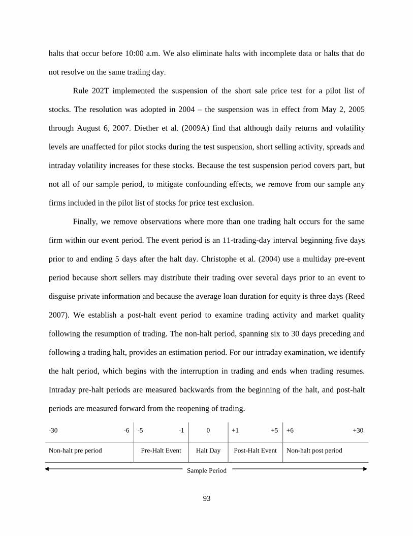
93
halts that occur before 10:00 a.m. We also eliminate halts with incomplete data or halts that do
not resolve on the same trading day.
Rule 202T implemented the suspension of the short sale price test for a pilot list of
stocks. The resolution was adopted in 2004 – the suspension was in effect from May 2, 2005
through August 6, 2007. Diether et al. (2009A) find that although daily returns and volatility
levels are unaffected for pilot stocks during the test suspension, short selling activity, spreads and
intraday volatility increases for these stocks. Because the test suspension period covers part, but
not all of our sample period, to mitigate confounding effects, we remove from our sample any
firms included in the pilot list of stocks for price test exclusion.
Finally, we remove observations where more than one trading halt occurs for the same
firm within our event period. The event period is an 11-trading-day interval beginning five days
prior to and ending 5 days after the halt day. Christophe et al. (2004) use a multiday pre-event
period because short sellers may distribute their trading over several days prior to an event to
disguise private information and because the average loan duration for equity is three days (Reed
2007). We establish a post-halt event period to examine trading activity and market quality
following the resumption of trading. The non-halt period, spanning six to 30 days preceding and
following a trading halt, provides an estimation period. For our intraday examination, we identify
the halt period, which begins with the interruption in trading and ends when trading resumes.
Intraday pre-halt periods are measured backwards from the beginning of the halt, and post-halt
periods are measured forward from the reopening of trading.
-30 -6 -5 -1 0 +1 +5 +6 +30
Non-halt pre period Pre-Halt Event Halt Day Post-Halt Event Non-halt post period
Sample Period

94
Daily price, trading volume, return, and market capitalization data are obtained from the
CRSP database. The Regulation SHO database, which was created in response to Rule 202T,
provides trade size and time stamps for short-selling transactions. TAQ trade and quote data is
used to examine intraday activity. Trade data is filtered to remove observations that occur
outside of normal market hours, and transactions with a non-positive price, or a condition code
other than zero. Quote data is filtered to retain observations that occur within normal market
hours and have a positive bid or ask size, price and spread.
REFERENCE GROUPS
We model our selection criteria for stocks related to halted firms on the methodology
implemented by Jiang et al. (2009). These researchers select a reference group for each of the
firms experiencing a trading halt by first identifying securities with the same 4-digit Standard
Industrial Classification (SIC) code. To define further the informational relationship, they
develop a scheme based on four dimensions: daily returns, trading volume, price volatility and
spreads.
Daily Returns
For each candidate stock, one with a SIC code that matches a halted stock, we obtain
daily returns from CRSP, regress them on the CRSP value-weighted return (the market model)
and capture the residual. A Pearson correlation is estimated between the residuals for the halted
stock and its industry contemporary stocks. Informational relatedness is established if the
correlation of the residuals is significant at the ten percent level.
95
Price Volatility
Highly correlated volatility measurements suggest a substantial degree of comovement in
informed trading between two stocks (Jiang et al. 2009). Daily volatility is estimated as the
squared residual from the market model (previously described for returns). Stocks are considered
a related firm if their squared residual has a Pearson correlation with that of a halted stock at or
above the ten percent significance level.
Trading Volume
We next apply a model developed by Ferris, Haugen, and Makhija (1988) and utilized by
Jiang et al. (2009) to separate the effects of firm or industry events from the effects produced by
market-wide, macro-economic conditions:
vi,t = αI + βivm,t + γi,t (1)
Where vi,t is the daily trading volume divided by the outstanding shares for stock i on day
t, vm,t is the total market volume divided by the total number of shares outstanding for all
securities on day t, and γi,t is the residual of the regression. For each stock, the regression is
estimated once for each sample year. Informationally related stocks are those whose Pearson
correlation is statistically significant at the ten percent level with the regression residual of the
halted stock.
Spreads
Using daily closing bid and ask prices, we estimate the average percentage spread {(ask –
bid) / share price} over 5-day increments for each year of the sample – producing approximately
50 spread measurements per year for each stock. Stocks are designated as informationally related
96
if their spread measurement is statistically correlated with that of the halted stock at the ten
percent level.
Industry counterpart firms are removed from the sample if they do not pass all four
information relatedness tests. Related firms are also eliminated if their average daily price and
trading volume during 2005 – 2006 is less than five dollars and 100 shares. Halts without a
related firm demonstrating statistically significant correlation for all four measures are dropped
from the sample. For halted firms with more than twenty related firms remaining after the
relatedness tests are applied, we select the fifteen most similar firms, based on market
capitalization, to retain in our sample of contemporary firms.
SUMMARY STATISTICS
The previously described filters produce a sample of 78 trading halts. Forty-seven of
these halts have reference firms that show significant correlation for daily returns, price
volatility, trading volume, and spreads. Table 1, Panels A through E, contains descriptive statics
for the trading halts; Table 2 and Table 3, Panels A through D, describe firm characteristics and
short selling activity for the halted and related firms, respectively. The sample of related firms
contains 172 unique firms, representing 188 related firm observations.
Table 1
Descriptive Statistics - Halts
This table describes our sample of 2005-2006 trading halts for NYSE-listed firms. Halts have
been filtered to remove observations that occur outside of market hours or before 10:00 a.m.,
where more than one halt occurs for a sample firms on the same day, halts that do not resolve on
the same trading day and multiple halts for the same firm within the 11-day event period, halts
for Rule 202T pilot stocks, observations for stocks whose average daily price and trading volume
during 2005 – 2006 was less than five dollars and 100 shares, and halts without a significantly
correlated reference firm.
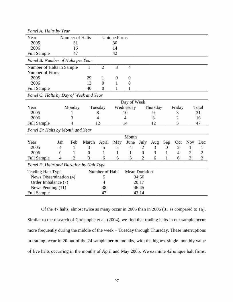
97
Panel A: Halts by Year
Year Number of Halts Unique Firms
2005 31 30
2006 16 14
Full Sample 47 42
Panel B: Number of Halts per Year
Number of Halts in Sample 1 2 3 4
Number of Firms
2005 29 1 0 0
2006 13 0 1 0
Full Sample 40 0 1 1
Panel C: Halts by Day of Week and Year
Day of Week
Year Monday Tuesday Wednesday Thursday Friday Total
2005 1 8 10 9 3 31
2006 3 4 4 3 2 16
Full Sample 4 12 14 12 5 47
Panel D: Halts by Month and Year
Month
Year Jan Feb March April May June July Aug Sep Oct Nov Dec
2005 4 1 3 5 5 4 2 3 0 2 1 1
2006 0 1 0 1 1 1 0 3 1 4 2 2
Full Sample 4 2 3 6 6 5 2 6 1 6 3 3
Panel E: Halts and Duration by Halt Type
Trading Halt Type Number of Halts Mean Duration
News Dissemination (4) 5 34:56
Order Imbalance (7) 4 20:17
News Pending (11) 38 46:45
Full Sample 47 43:14
Of the 47 halts, almost twice as many occur in 2005 than in 2006 (31 as compared to 16).
Similar to the research of Christophe et al. (2004), we find that trading halts in our sample occur
more frequently during the middle of the week – Tuesday through Thursday. These interruptions
in trading occur in 20 out of the 24 sample period months, with the highest single monthly value
of five halts occurring in the months of April and May 2005. We examine 42 unique halt firms,
98
40 of which experience a single halt during the sample period and 2 different firms that
experience 3 or 4 halts each.
The halts in our study are primarily (81 percent) implemented due to pending news. The
mean duration of all sample halts is just over 43 minutes. Although the duration of trading halts
reported by previous research, including Lee et al. (1994), Corwin and Lipson (2000), and
Christie et al. (2002), is greater on average and for each halt type, our findings coincide with the
ranking of halt types by length: news pending halts have the longest duration and order
imbalance halts, the shortest.
Summary statistics for both halted and related firms suggest a substantial variation in the
size of sample firms, stock prices, and trading volume, with generally higher average values in
2006 as compared to 2005. However, the range in average security prices, trading volume, and
returns is substantially larger for the sample of related firms as compared to halted firms, and the
variability in volume and market capitalization is much higher for both samples in 2006. The
firms, on average, demonstrate positive returns over the two-year period examined. When both
sets of firms are categorized according to the year-end capitalization portfolio assignments
established by CRSP, we find, similar to Christophe et al. (2004) that large firms are more
heavily represented in our sample of halt firms. There are fewer halt firms in the lower market
capitalization deciles, perhaps due, in part, to our data filter that eliminates trading halts for any
stock whose average daily price during the sample period is less than five dollars. In contrast, the
related firms are distributed throughout all ten of the market capitalization deciles. Both samples
demonstrate the largest number of firms, over 20 percent of observations, in decile six.
We examine short-selling levels for our halt and related stocks during the 2005 – 2006
sample period. For each exchange, we report both short volume as a percentage of the total
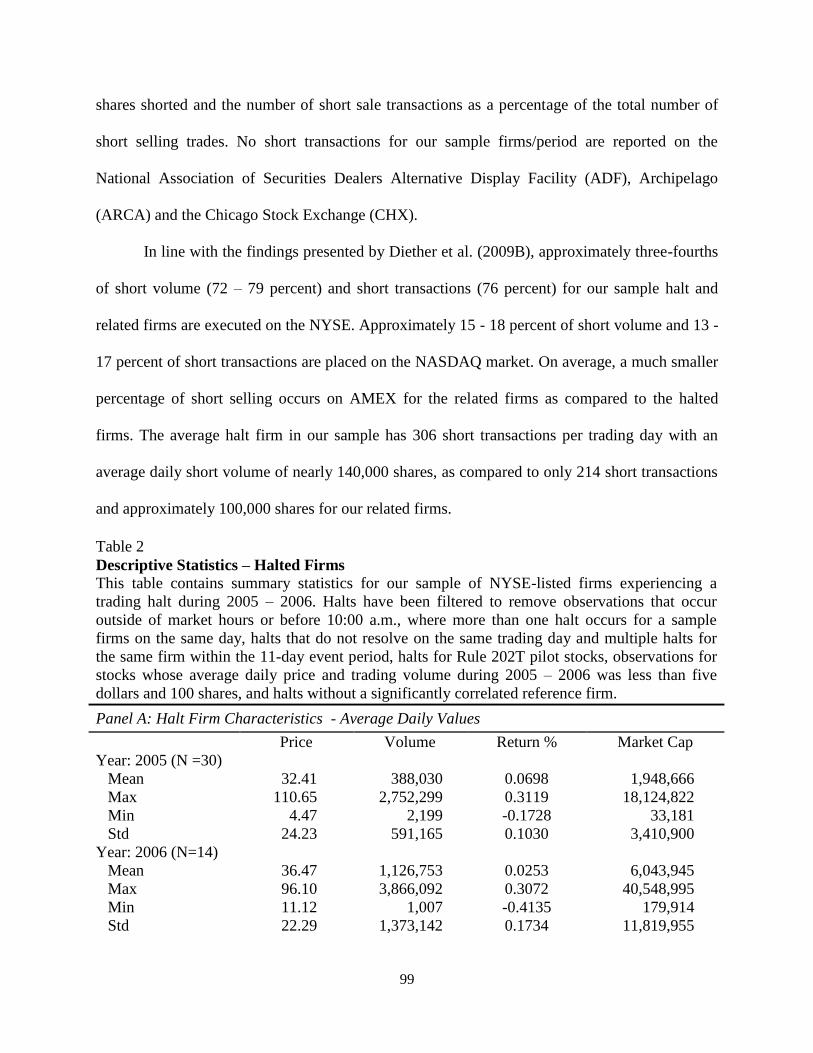
99
shares shorted and the number of short sale transactions as a percentage of the total number of
short selling trades. No short transactions for our sample firms/period are reported on the
National Association of Securities Dealers Alternative Display Facility (ADF), Archipelago
(ARCA) and the Chicago Stock Exchange (CHX).
In line with the findings presented by Diether et al. (2009B), approximately three-fourths
of short volume (72 – 79 percent) and short transactions (76 percent) for our sample halt and
related firms are executed on the NYSE. Approximately 15 - 18 percent of short volume and 13 -
17 percent of short transactions are placed on the NASDAQ market. On average, a much smaller
percentage of short selling occurs on AMEX for the related firms as compared to the halted
firms. The average halt firm in our sample has 306 short transactions per trading day with an
average daily short volume of nearly 140,000 shares, as compared to only 214 short transactions
and approximately 100,000 shares for our related firms.
Table 2
Descriptive Statistics – Halted Firms
This table contains summary statistics for our sample of NYSE-listed firms experiencing a
trading halt during 2005 – 2006. Halts have been filtered to remove observations that occur
outside of market hours or before 10:00 a.m., where more than one halt occurs for a sample
firms on the same day, halts that do not resolve on the same trading day and multiple halts for
the same firm within the 11-day event period, halts for Rule 202T pilot stocks, observations for
stocks whose average daily price and trading volume during 2005 – 2006 was less than five
dollars and 100 shares, and halts without a significantly correlated reference firm.
Panel A: Halt Firm Characteristics - Average Daily Values
Price Volume Return % Market Cap
Year: 2005 (N =30)
Mean 32.41 388,030 0.0698 1,948,666
Max 110.65 2,752,299 0.3119 18,124,822
Min 4.47 2,199 -0.1728 33,181
Std 24.23 591,165 0.1030 3,410,900
Year: 2006 (N=14)
Mean 36.47 1,126,753 0.0253 6,043,945
Max 96.10 3,866,092 0.3072 40,548,995
Min 11.12 1,007 -0.4135 179,914
Std 22.29 1,373,142 0.1734 11,819,955
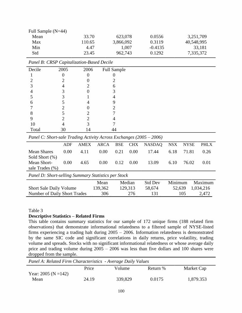
100
Full Sample (N=44)
Mean 33.70 623,078 0.0556 3,251,709
Max 110.65 3,866,092 0.3119 40,548,995
Min 4.47 1,007 -0.4135 33,181
Std 23.45 962,743 0.1292 7,335,372
Panel B: CRSP Capitalization-Based Decile
Decile 2005 2006 Full Sample
1 0 0 0
2 2 0 2
3 4 2 6
4 3 0 3
5 3 1 4
6 5 4 9
7 2 0 2
8 5 2 7
9 2 2 4
10 4 3 7
Total 30 14 44
Panel C: Short-sale Trading Activity Across Exchanges (2005 – 2006)
ADF AMEX ARCA BSE CHX NASDAQ NSX NYSE PHLX
Mean Shares
Sold Short (%)
0.00 4.11 0.00 0.21 0.00 17.44 6.18 71.81 0.26
Mean Short-
sale Trades (%)
0.00 4.65 0.00 0.12 0.00 13.09 6.10 76.02 0.01
Panel D: Short-selling Summary Statistics per Stock
Mean Median Std Dev Minimum Maximum
Short Sale Daily Volume 139,362 129,313 58,674 52,639 1,034,216
Number of Daily Short Trades 306 276 131 105 2,472
Table 3
Descriptive Statistics – Related Firms
This table contains summary statistics for our sample of 172 unique firms (188 related firm
observations) that demonstrate informational relatedness to a filtered sample of NYSE-listed
firms experiencing a trading halt during 2005 – 2006. Information relatedness is demonstrated
by the same SIC code and significant correlations in daily returns, price volatility, trading
volume and spreads. Stocks with no significant informational relatedness or whose average daily
price and trading volume during 2005 – 2006 was less than five dollars and 100 shares were
dropped from the sample.
Panel A: Related Firm Characteristics - Average Daily Values
Price Volume Return % Market Cap
Year: 2005 (N =142)
Mean 24.19 339,829 0.0175 1,879.353
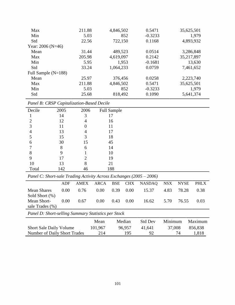
101
Max 211.88 4,846,502 0.5471 35,625,501
Min 5.03 852 -0.3233 1,979
Std 22.56 722,150 0.1168 4,893,932
Year: 2006 (N=46)
Mean 31.44 489,523 0.0514 3,286,848
Max 205.98 4,619,097 0.2142 35,217,897
Min 5.95 1,953 -0.1681 13,630
Std 33.24 1,064,233 0.0759 7,461,652
Full Sample (N=188)
Mean 25.97 376,456 0.0258 2,223,740
Max 211.88 4,846,502 0.5471 35,625,501
Min 5.03 852 -0.3233 1,979
Std 25.68 818,492 0.1090 5,641,374
Panel B: CRSP Capitalization-Based Decile
Decile 2005 2006 Full Sample
1 14 3 17
2 12 4 16
3 11 0 11
4 13 4 17
5 15 3 18
6 30 15 45
7 8 6 14
8 9 1 10
9 17 2 19
10 13 8 21
Total 142 46 188
Panel C: Short-sale Trading Activity Across Exchanges (2005 – 2006)
ADF AMEX ARCA BSE CHX NASDAQ NSX NYSE PHLX
Mean Shares
Sold Short (%)
0.00 0.76 0.00 0.39 0.00 15.37 4.83 78.28 0.38
Mean Short-
sale Trades (%)
0.00 0.67 0.00 0.43 0.00 16.62 5.70 76.55 0.03
Panel D: Short-selling Summary Statistics per Stock
Mean Median Std Dev Minimum Maximum
Short Sale Daily Volume 101,967 96,957 41,641 37,008 856,838
Number of Daily Short Trades 214 195 92 74 1,818
102
RESULTS
Daily Short Metrics
To detect changes in the daily activity of short sellers surrounding trading halts, we track
the average number of trades, trade size, and volume for short transactions for our sample of
informationally related firms in the pre-halt period (days -5 through -1), the halt day (day 0), the
post-halt period (days +1 through +5), and the estimation period (days -30 through -6 and +6
through +30). We also calculate the short interest ratio, relative short selling, and abnormal short
selling metrics for each of these periods. The short interest ratio is described by Angel et al.
(2003), as the number of shares sold short to shares outstanding. Relative short selling is
calculated by dividing the number of shares shorted by the number of shares traded (Christophe
et al., 2004; and Diether et al., 2009B). Abnormal short selling is the percentage difference
between the average daily shares sold short during the pre, halt, or post period and the average
daily number of shares sold short during the estimation period (Lee et al., 1994; Corwin and
Lipson, 2000; Christie et al., 2002, Christophe et al., 2004; and Christophe et al., 2010). For each
short selling metric, a difference value is computed to determine if corresponding pre-halt, halt,
and post-halt values differ from estimation period levels. Significance is determined using the
Wilcoxon signed-rank test, which allows us to compare measurements on our sample without
relying on an assumption of normality.
Our hypothesis concerning the behavior of short sellers surrounding trading halts states:
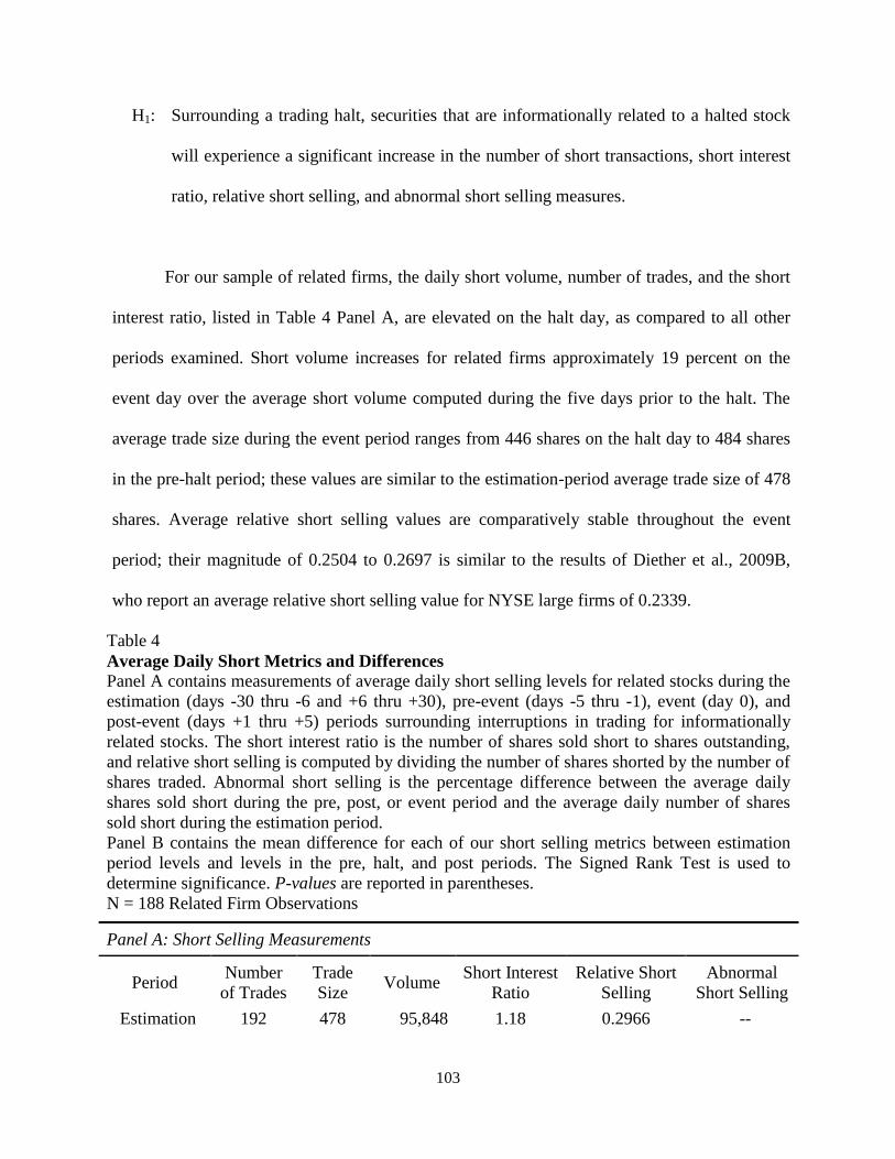
103
H1: Surrounding a trading halt, securities that are informationally related to a halted stock
will experience a significant increase in the number of short transactions, short interest
ratio, relative short selling, and abnormal short selling measures.
For our sample of related firms, the daily short volume, number of trades, and the short
interest ratio, listed in Table 4 Panel A, are elevated on the halt day, as compared to all other
periods examined. Short volume increases for related firms approximately 19 percent on the
event day over the average short volume computed during the five days prior to the halt. The
average trade size during the event period ranges from 446 shares on the halt day to 484 shares
in the pre-halt period; these values are similar to the estimation-period average trade size of 478
shares. Average relative short selling values are comparatively stable throughout the event
period; their magnitude of 0.2504 to 0.2697 is similar to the results of Diether et al., 2009B,
who report an average relative short selling value for NYSE large firms of 0.2339.
Table 4
Average Daily Short Metrics and Differences
Panel A contains measurements of average daily short selling levels for related stocks during the
estimation (days -30 thru -6 and +6 thru +30), pre-event (days -5 thru -1), event (day 0), and
post-event (days +1 thru +5) periods surrounding interruptions in trading for informationally
related stocks. The short interest ratio is the number of shares sold short to shares outstanding,
and relative short selling is computed by dividing the number of shares shorted by the number of
shares traded. Abnormal short selling is the percentage difference between the average daily
shares sold short during the pre, post, or event period and the average daily number of shares
sold short during the estimation period.
Panel B contains the mean difference for each of our short selling metrics between estimation
period levels and levels in the pre, halt, and post periods. The Signed Rank Test is used to
determine significance. P-values are reported in parentheses.
N = 188 Related Firm Observations
Panel A: Short Selling Measurements
Period Number
of Trades
Trade
Size Volume
Short Interest
Ratio
Relative Short
Selling
Abnormal
Short Selling
Estimation 192 478 95,848 1.18 0.2966 --
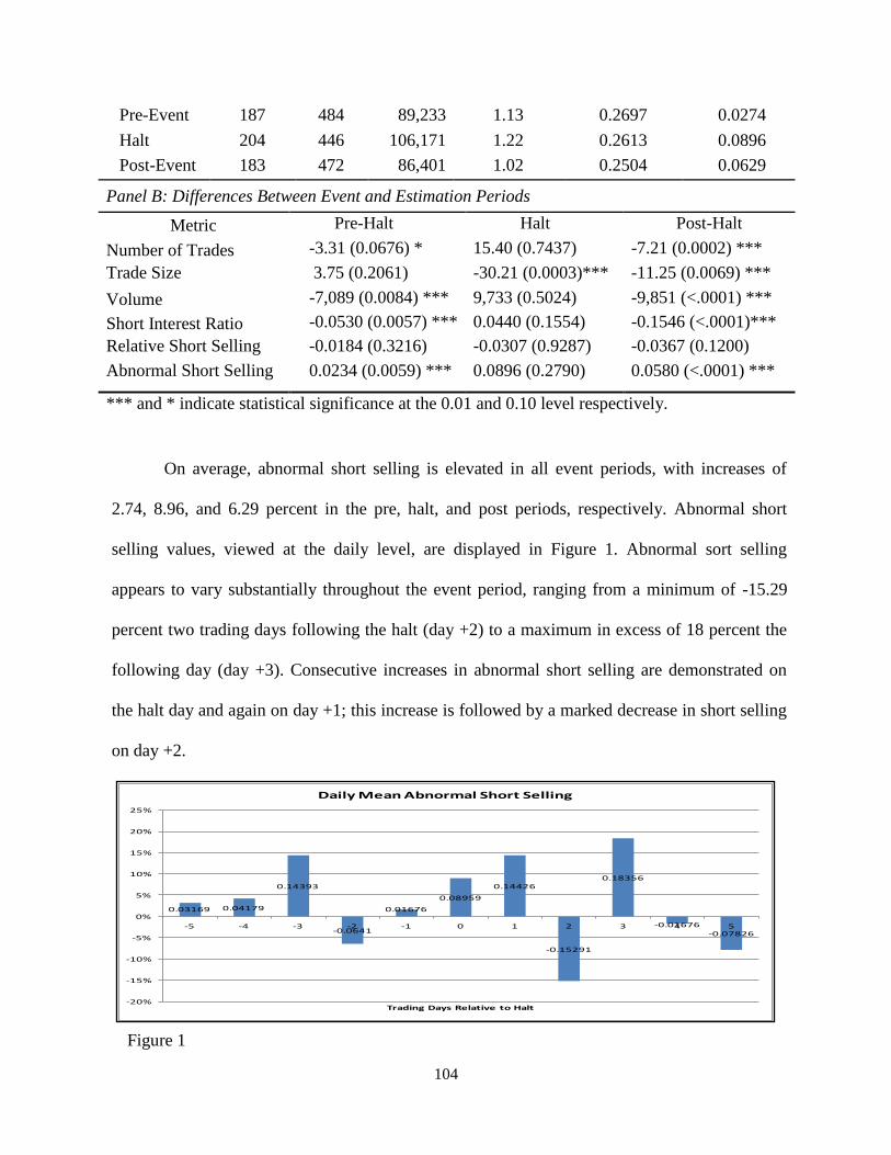
104
Pre-Event 187 484 89,233 1.13 0.2697 0.0274
Halt 204 446 106,171 1.22 0.2613 0.0896
Post-Event 183 472 86,401 1.02 0.2504 0.0629
Panel B: Differences Between Event and Estimation Periods
Metric Pre-Halt Halt Post-Halt
Number of Trades -3.31 (0.0676) * 15.40 (0.7437) -7.21 (0.0002) ***
Trade Size 3.75 (0.2061) -30.21 (0.0003)*** -11.25 (0.0069) ***
Volume -7,089 (0.0084) *** 9,733 (0.5024) -9,851 (<.0001) ***
Short Interest Ratio -0.0530 (0.0057) *** 0.0440 (0.1554) -0.1546 (<.0001)***
Relative Short Selling -0.0184 (0.3216) -0.0307 (0.9287) -0.0367 (0.1200)
Abnormal Short Selling 0.0234 (0.0059) *** 0.0896 (0.2790) 0.0580 (<.0001) ***
*** and * indicate statistical significance at the 0.01 and 0.10 level respectively.
On average, abnormal short selling is elevated in all event periods, with increases of
2.74, 8.96, and 6.29 percent in the pre, halt, and post periods, respectively. Abnormal short
selling values, viewed at the daily level, are displayed in Figure 1. Abnormal sort selling
appears to vary substantially throughout the event period, ranging from a minimum of -15.29
percent two trading days following the halt (day +2) to a maximum in excess of 18 percent the
following day (day +3). Consecutive increases in abnormal short selling are demonstrated on
the halt day and again on day +1; this increase is followed by a marked decrease in short selling
on day +2.
Figure 1
0.03169 0.04179
0.14393
-0.0641
0.01676
0.08959
0.14426
-0.15291
0.18356
-0.01676
-0.07826
-20%
-15%
-10%
-5%
0%
5%
10%
15%
20%
25%
-5 -4 -3 -2 -1 0 1 2 3 4 5
Trading Days Relative to Halt
Daily Mean Abnormal Short Selling
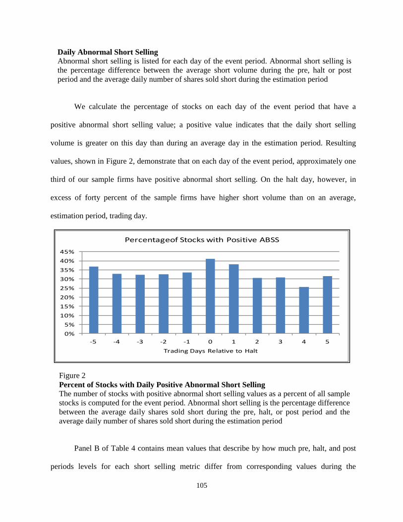
105
Daily Abnormal Short Selling
Abnormal short selling is listed for each day of the event period. Abnormal short selling is
the percentage difference between the average short volume during the pre, halt or post
period and the average daily number of shares sold short during the estimation period
We calculate the percentage of stocks on each day of the event period that have a
positive abnormal short selling value; a positive value indicates that the daily short selling
volume is greater on this day than during an average day in the estimation period. Resulting
values, shown in Figure 2, demonstrate that on each day of the event period, approximately one
third of our sample firms have positive abnormal short selling. On the halt day, however, in
excess of forty percent of the sample firms have higher short volume than on an average,
estimation period, trading day.
Figure 2
Percent of Stocks with Daily Positive Abnormal Short Selling
The number of stocks with positive abnormal short selling values as a percent of all sample
stocks is computed for the event period. Abnormal short selling is the percentage difference
between the average daily shares sold short during the pre, halt, or post period and the
average daily number of shares sold short during the estimation period
Panel B of Table 4 contains mean values that describe by how much pre, halt, and post
periods levels for each short selling metric differ from corresponding values during the
0%
5%
10%
15%
20%
25%
30%
35%
40%
45%
-5 -4 -3 -2 -1 0 1 2 3 4 5
Trading Days Relative to Halt
Percentageof Stocks with Positive ABSS
106
estimation period. A significant decrease in the number of trades, short volume, and the short
interest ratio occurs in both the pre- and post-halt periods (the five days preceding and
following the event day). This result indicates that short sellers modify their behavior in regards
to our sample of firms in the days leading up to and following a halt in trading for a related
industry member by submitting fewer and smaller short transactions. The only short-selling
measurement that demonstrates a significant difference on the halt day is trade size, which on
average is thirty shares smaller than the mean trade size during the estimation period. Difference
values for relative short selling are insignificant for all three of the event periods; a lack of
significance suggests that for our sample of related firms, the trading halt event does not
substantially alter the relation between their short and overall trading volume. An increase in
short selling for related firms is substantiated by the difference statistic for abnormal short
selling – this measurement is two to six percent higher during the pre- and post-halt intervals.
However, no significant increase in abnormal short selling over estimation period levels is
identified on the halt day.
Market microstructure research demonstrates that short sellers use their superior
knowledge to extract gains in the market surrounding informational events. We build upon this
finding to determine, by examining the relation between pre- and post-event returns and pre-
event short selling levels, if informed market participants increase their short selling activity for
related firms prior to interruptions in trading. Using the following equation, we examine short
selling levels while controlling for other variables that might influence short selling activity
(following Christophe et al., 2010):
ABSS(-5,-1)i = αi + β1Log(P0)i + β2CAR(-5,-1)i + β3MOMi + β4CAR(0,1)i + εi (2)
107
The dependent variable, ABSS(-5,-1) represents abnormal short-selling during the five
days preceding the halt. LogP(0) is the natural logarithm of a related firm’s share price on the
event day; this variable controls for the positive link between a stock’s price and the willingness
of market participants to short the stock.10
CAR(-5,-1) is the cumulative abnormal return earned
during the five day pre-halt period – the halted firm’s total return over the five days preceding
the halt minus the median five-day cumulative return during the estimation period. MOM
represents momentum, which controls for long-term share price movement. Momentum is
calculated as the related firm’s six-month cumulative return ending 30 days before the halt,
minus the return on the NYSE equally weighted portfolio during the same period. CAR(0,1) is
the related firm’s holding period return from day 0 to day 1, minus the median holding period
return during the estimation period; this variable represents the market’s assessment of the
economic value of the information associated with an interruption in trading.
Using ordinary least squares to model a regression equation relies on the assumption that
the error terms have uniform variances across all observations. We use the Shapiro-Wilk test on
each regression input data set to ensure that the assumption of normality holds. The null
hypothesis for this statistical test is that a population is distributed normally. If the test produces
a p-value less than the designated alpha level of 0.10, then the null hypothesis of normality can
be rejected. When this occurs, we report results using errors adjusted to control for
heteroscedasticity and serial correlation of the residuals.
Table 5, Panel A displays the correlation matrix for the regression variables. The
correlation values demonstrate two significant relations between returns and short selling.
Returns in the five-day pre-halt period are inversely related to pre-halt abnormal short selling
10
Refer to D’Avolio, (2002) who shows that the majority of stocks that are difficult to short are priced less than five
dollars and that the holdings of institutional investors, who lend stocks for shorting, are biased towards large, liquid
stocks.
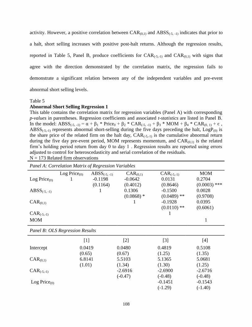
108
activity. However, a positive correlation between CAR(0,1) and ABSS(-5, -1) indicates that prior to
a halt, short selling increases with positive post-halt returns. Although the regression results,
reported in Table 5, Panel B, produce coefficients for CAR(-5,-1) and CAR(0,1) with signs that
agree with the direction demonstrated by the correlation matrix, the regression fails to
demonstrate a significant relation between any of the independent variables and pre-event
abnormal short selling levels.
Table 5
Abnormal Short Selling Regression 1
This table contains the correlation matrix for regression variables (Panel A) with corresponding
p-values in parentheses. Regression coefficients and associated t-statistics are listed in Panel B.
In the model: ABSS(-5, -1) = α + β1 * Price0 + β2 * CAR(-5, -1) + β3 * MOM + β4 * CAR(0, 1) + є ,
ABSS(-5,-1) represents abnormal short-selling during the five days preceding the halt, LogP(0) is
the share price of the related firm on the halt day, CAR(-5,-1) is the cumulative abnormal return
during the five day pre-event period, MOM represents momentum, and CAR(0,1) is the related
firm’s holding period return from day 0 to day 1 . Regression results are reported using errors
adjusted to control for heteroscedasticity and serial correlation of the residuals.
N = 173 Related firm observations
Panel A: Correlation Matrix of Regression Variables
Log Price(0) ABSS(-5, -1) CAR(0,1) CAR(-5,-1) MOM
Log Price(0) 1 -0.1198
(0.1164)
-0.0642
(0.4012)
0.0131
(0.8646)
0.2704
(0.0003) ***
ABSS(-5, -1) 1 0.1306
(0.0868) *
-0.1500
(0.0489) **
0.0028
(0.9708)
CAR(0,1) 1 -0.1928
(0.0110) **
0.0395
(0.6061)
CAR(-5,-1) 1
MOM 1
Panel B: OLS Regression Results
[1] [2] [3] [4]
Intercept 0.0419
(0.65)
0.0480
(0.67)
0.4819
(1.25)
0.5108
(1.35)
CAR(0,1) 6.8141
(1.01)
5.5103
(1.34)
5.1365
(1.30)
5.0681
(1.25)
CAR(-5,-1)
-2.6916
(-0.47)
-2.6900
(-0.48)
-2.6716
(-0.48)
Log Price(0)
-0.1451
(-1.29)
-0.1543
(-1.40)
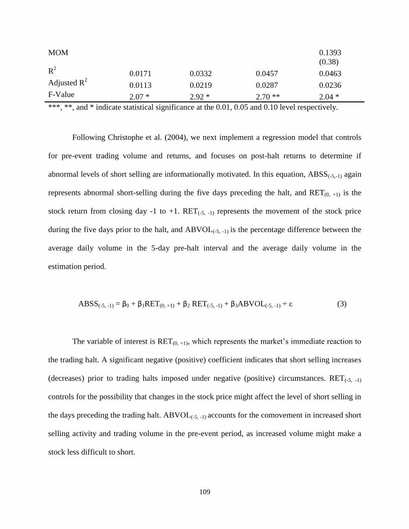
109
MOM
0.1393
(0.38)
R2 0.0171 0.0332 0.0457 0.0463
Adjusted R2 0.0113 0.0219 0.0287 0.0236
F-Value 2.07 * 2.92 * 2.70 ** 2.04 *
***, **, and * indicate statistical significance at the 0.01, 0.05 and 0.10 level respectively.
Following Christophe et al. (2004), we next implement a regression model that controls
for pre-event trading volume and returns, and focuses on post-halt returns to determine if
abnormal levels of short selling are informationally motivated. In this equation, ABSS(-5,-1) again
represents abnormal short-selling during the five days preceding the halt, and RET(0, +1) is the
stock return from closing day -1 to +1. RET(-5, -1) represents the movement of the stock price
during the five days prior to the halt, and ABVOL(-5, -1) is the percentage difference between the
average daily volume in the 5-day pre-halt interval and the average daily volume in the
estimation period.
ABSS(-5, -1) = β0 + β1RET(0, +1) + β2 RET(-5, -1) + β3ABVOL(-5, -1) + ε (3)
The variable of interest is RET(0, +1), which represents the market’s immediate reaction to
the trading halt. A significant negative (positive) coefficient indicates that short selling increases
(decreases) prior to trading halts imposed under negative (positive) circumstances. RET(-5, -1)
controls for the possibility that changes in the stock price might affect the level of short selling in
the days preceding the trading halt. ABVOL(-5, -1) accounts for the comovement in increased short
selling activity and trading volume in the pre-event period, as increased volume might make a
stock less difficult to short.
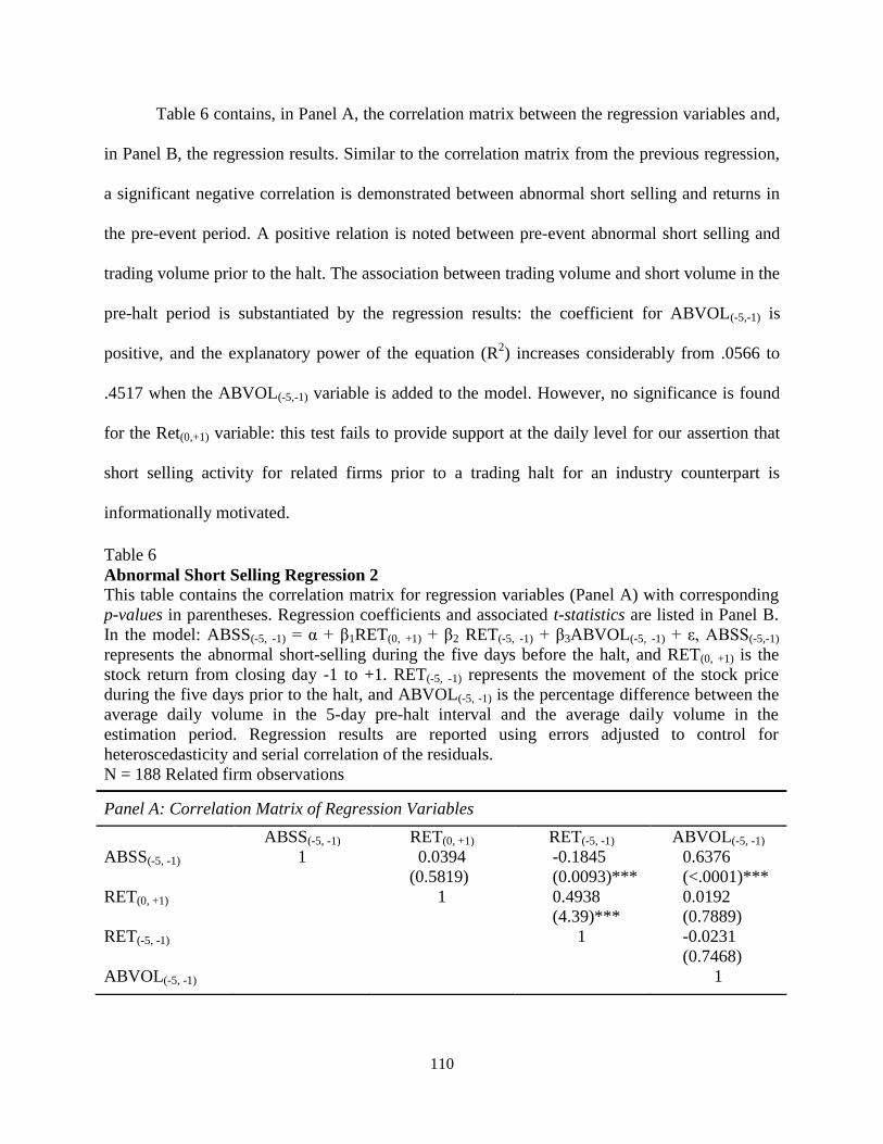
110
Table 6 contains, in Panel A, the correlation matrix between the regression variables and,
in Panel B, the regression results. Similar to the correlation matrix from the previous regression,
a significant negative correlation is demonstrated between abnormal short selling and returns in
the pre-event period. A positive relation is noted between pre-event abnormal short selling and
trading volume prior to the halt. The association between trading volume and short volume in the
pre-halt period is substantiated by the regression results: the coefficient for ABVOL(-5,-1) is
positive, and the explanatory power of the equation (R2) increases considerably from .0566 to
.4517 when the ABVOL(-5,-1) variable is added to the model. However, no significance is found
for the Ret(0,+1) variable: this test fails to provide support at the daily level for our assertion that
short selling activity for related firms prior to a trading halt for an industry counterpart is
informationally motivated.
Table 6
Abnormal Short Selling Regression 2
This table contains the correlation matrix for regression variables (Panel A) with corresponding
p-values in parentheses. Regression coefficients and associated t-statistics are listed in Panel B.
In the model: ABSS(-5, -1) = α + β1RET(0, +1) + β2 RET(-5, -1) + β3ABVOL(-5, -1) + ε, ABSS(-5,-1)
represents the abnormal short-selling during the five days before the halt, and RET(0, +1) is the
stock return from closing day -1 to +1. RET(-5, -1) represents the movement of the stock price
during the five days prior to the halt, and ABVOL(-5, -1) is the percentage difference between the
average daily volume in the 5-day pre-halt interval and the average daily volume in the
estimation period. Regression results are reported using errors adjusted to control for
heteroscedasticity and serial correlation of the residuals.
N = 188 Related firm observations
Panel A: Correlation Matrix of Regression Variables
ABSS(-5, -1) RET(0, +1) RET(-5, -1) ABVOL(-5, -1)
ABSS(-5, -1) 1 0.0394
(0.5819)
-0.1845
(0.0093)***
0.6376
(<.0001)***
RET(0, +1) 1 0.4938
(4.39)***
0.0192
(0.7889)
RET(-5, -1) 1 -0.0231
(0.7468)
ABVOL(-5, -1) 1
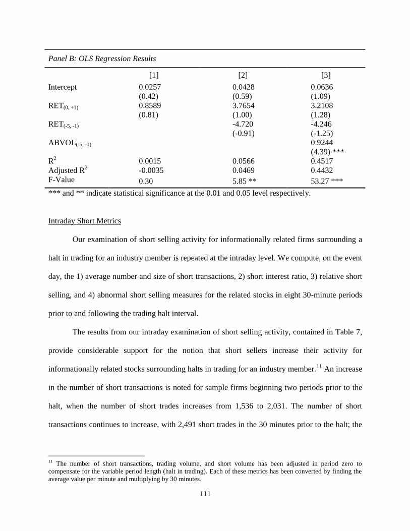
111
Intraday Short Metrics
Our examination of short selling activity for informationally related firms surrounding a
halt in trading for an industry member is repeated at the intraday level. We compute, on the event
day, the 1) average number and size of short transactions, 2) short interest ratio, 3) relative short
selling, and 4) abnormal short selling measures for the related stocks in eight 30-minute periods
prior to and following the trading halt interval.
The results from our intraday examination of short selling activity, contained in Table 7,
provide considerable support for the notion that short sellers increase their activity for
informationally related stocks surrounding halts in trading for an industry member.11
An increase
in the number of short transactions is noted for sample firms beginning two periods prior to the
halt, when the number of short trades increases from 1,536 to 2,031. The number of short
transactions continues to increase, with 2,491 short trades in the 30 minutes prior to the halt; the
11
The number of short transactions, trading volume, and short volume has been adjusted in period zero to
compensate for the variable period length (halt in trading). Each of these metrics has been converted by finding the
average value per minute and multiplying by 30 minutes.
Panel B: OLS Regression Results
[1] [2] [3]
Intercept 0.0257
(0.42)
0.0428
(0.59)
0.0636
(1.09)
RET(0, +1) 0.8589
(0.81)
3.7654
(1.00)
3.2108
(1.28)
RET(-5, -1)
-4.720
(-0.91)
-4.246
(-1.25)
ABVOL(-5, -1)
0.9244
(4.39) ***
R2 0.0015 0.0566 0.4517
Adjusted R2 -0.0035 0.0469 0.4432
F-Value 0.30 5.85 ** 53.27 ***
*** and ** indicate statistical significance at the 0.01 and 0.05 level respectively.
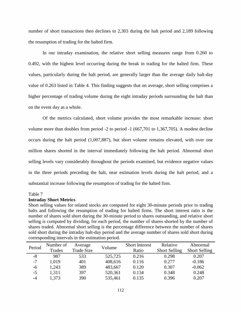
112
number of short transactions then declines to 2,303 during the halt period and 2,189 following
the resumption of trading for the halted firm.
In our intraday examination, the relative short selling measures range from 0.260 to
0.492, with the highest level occurring during the break in trading for the halted firm. These
values, particularly during the halt period, are generally larger than the average daily halt-day
value of 0.263 listed in Table 4. This finding suggests that on average, short selling comprises a
higher percentage of trading volume during the eight intraday periods surrounding the halt than
on the event day as a whole.
Of the metrics calculated, short volume provides the most remarkable increase: short
volume more than doubles from period -2 to period -1 (667,701 to 1,367,705). A modest decline
occurs during the halt period (1,007,887), but short volume remains elevated, with over one
million shares shorted in the interval immediately following the halt period. Abnormal short
selling levels vary considerably throughout the periods examined, but evidence negative values
in the three periods preceding the halt, near estimation levels during the halt period, and a
substantial increase following the resumption of trading for the halted firm.
Table 7
Intraday Short Metrics
Short selling values for related stocks are computed for eight 30-minute periods prior to trading
halts and following the resumption of trading for halted firms. The short interest ratio is the
number of shares sold short during the 30-minute period to shares outstanding, and relative short
selling is computed by dividing, for each period, the number of shares shorted by the number of
shares traded. Abnormal short selling is the percentage difference between the number of shares
sold short during the intraday halt-day period and the average number of shares sold short during
corresponding intervals in the estimation period.
Period Number of
Trades
Average
Trade Size Volume
Short Interest
Ratio
Relative
Short Selling
Abnormal
Short Selling
-8 987 533 525,725 0.216 0.298 0.207
-7 1,019 401 408,616 0.116 0.277 -0.186
-6 1,243 389 483,667 0.120 0.307 -0.062
-5 1,311 397 520,361 0.134 0.348 0.248
-4 1,373 390 535,461 0.135 0.396 0.207
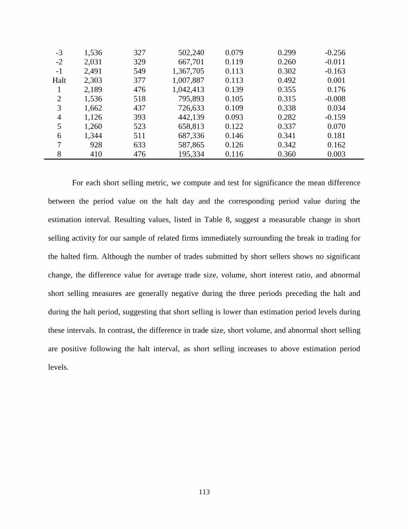
113
-3 1,536 327 502,240 0.079 0.299 -0.256
-2 2,031 329 667,701 0.119 0.260 -0.011
-1 2,491 549 1,367,705 0.113 0.302 -0.163
Halt 2,303 377 1,007,887 0.113 0.492 0.001
1 2,189 476 1,042,413 0.139 0.355 0.176
2 1,536 518 795,893 0.105 0.315 -0.008
3 1,662 437 726,633 0.109 0.338 0.034
4 1,126 393 442,139 0.093 0.282 -0.159
5 1,260 523 658,813 0.122 0.337 0.070
6 1,344 511 687,336 0.146 0.341 0.181
7 928 633 587,865 0.126 0.342 0.162
8 410 476 195,334 0.116 0.360 0.003
For each short selling metric, we compute and test for significance the mean difference
between the period value on the halt day and the corresponding period value during the
estimation interval. Resulting values, listed in Table 8, suggest a measurable change in short
selling activity for our sample of related firms immediately surrounding the break in trading for
the halted firm. Although the number of trades submitted by short sellers shows no significant
change, the difference value for average trade size, volume, short interest ratio, and abnormal
short selling measures are generally negative during the three periods preceding the halt and
during the halt period, suggesting that short selling is lower than estimation period levels during
these intervals. In contrast, the difference in trade size, short volume, and abnormal short selling
are positive following the halt interval, as short selling increases to above estimation period
levels.
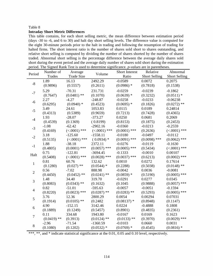
114
Table 8
Intraday Short Metric Differences
This table contains, for each short selling metric, the mean difference between estimation period
(days -30 to -6, and 6 to 30) and halt day short selling levels. The difference value is computed for
the eight 30-minute periods prior to the halt in trading and following the resumption of trading for
halted firms. The short interest ratio is the number of shares sold short to shares outstanding, and
relative short selling is computed by dividing the number of shares shorted by the number of shares
traded. Abnormal short selling is the percentage difference between the average daily shares sold
short during the event period and the average daily number of shares sold short during the estimation
period. The Signed Rank Test is used to determine significance. p-values are in parentheses.
Period Number of
Trades
Average
Trade Size Volume
Short Interest
Ratio
Relative
Short Selling
Abnormal
Short Selling
-8 1.89
(0.9896)
16.13
(0.5557)
2492.29
(0.2611)
-0.0589
(0.0986) *
0.0072
(0.7818)
0.2075
(0.1538)
-7 5.29
(0.7647)
-70.31
(0.0481) **
231.731
(0.1070)
-0.0259
(0.0639) *
-0.0239
(0.3232)
-0.1862
(0.0511) *
-6 2.27
(0.6295)
-4.27
(0.0940) *
-248.87
(0.4523)
-0.0258
(0.0695) *
-0.0233
(0.1826)
-0.06238
(0.0272) **
-5 3.49
(0.4313)
24.61
(0.5389)
1053.83
(0.9659)
0.0115
(0.7213)
0.0189
(0.7428)
0.24814
(0.4365)
-4 1.93
(0.4539)
-28.07
(0.1369)
-373.27
( 0.8199)
0.0250
(0.8153)
0.0681
(0.1875)
0.2069
(0.2453)
-3 -1.08
(0.4169)
-62.42
(<.0001) ***
-2902.16
(<.0001) ***
-0.0360
(0.0001) ***
-0.0213
(0.2636)
-0.2559
(<.0001) ***
-2 3.18
(0.5135)
-125.60
(<.0001) ***
-1558.11
( 0.0934) *
-0.0180
(0.0091) ***
-0.0497
(0.0098) ***
-0.0112
(0.0062) ***
-1 1.88
(0.4805)
-38.18
(0.0001) ***
2372.11
(0.0057) ***
-0.0276
(0.0005) ***
-0.0119
(0.5434)
-0.1630
(<.0001) ***
Halt 0.75
(0.5408)
-122.81
(<.0001) ***
-3694.45
(0.0028) ***
-0.1333
(0.0037) ***
-0.0010
(0.6213)
0.00107
(0.0002) ***
1 0.81
(0.1280)
60.76
(0.027) **
132.62
(0.0544) *
0.0010
(0.2288)
0.0272
(0.5038)
0.17614
(0.0148) **
2 0.56
(0.4450)
-7.02
(0.0452) **
888.98
(0.0241) **
-0.0042
(0.0859) *
0.0036
(0.5190)
-0.0081
(0.0005) ***
3 1.48
(0.8083)
34.40
(0.0343) **
319.70
(0.1632)
-0.0291
(0.1045
0.0277
(0.9888)
0.0345
(0.0057) ***
4 0.82
(0.8220)
-51.01
(0.0023) ***
-595.63
(0.0287) **
-0.0057
(0.0283) **
-0.0051
(0.5293)
-0.1594
(0.0005) ***
5 3.76
(0.1914)
12.36
(0.0105) **
2800.29
(0.2482
0.0054
(0.08137) *
0.00294
(0.8948)
0.07031
(0.1147)
6 4.90
(0.1889)
-152.15
(0.1249)
3142.46
(0.5457)
0.0224
(0.8901)
-0.4888
(0.4835)
0.1808
(0.2361)
7 0.11
(0.0419) **
334.68
(0.3913)
1943.80
(0.0124) **
-0.0167
(0.0133) **
0.0169
(0.3970)
0.1623
(0.0029) ***
8 -2.96
(0.1080)
-71.54
(0.1202)
-1360.59
(0.0532) *
-0.0103
(0.0769) *
0.0660
(0.4545)
0.0031
(0.0816) *
***, **, and * indicate statistical significance at the 0.01, 0.05 and 0.10 level, respectively.
115
Hypothesis 1 purports that short sellers increase their activity for informationally related
firms surrounding a halt in trading for an industry member. Our investigation of daily and
intraday short metrics evidences a measurable change in short seller behavior for our sample of
related firms. However, instead of the anticipated increase, it appears that short sellers reduce
their activity surrounding the halt event. During the 5-day pre- and post-halt periods, short sellers
submit fewer trades at a smaller average trade size, resulting in a decrease in short volume during
these intervals. A decline is short activity is also detected at the intraday level, as short selling
metrics, including average trade size, volume, the short interest ratio and abnormal short selling,
decrease prior to the halt period. An increase in shorting is identified in the intraday period
immediately following the resumption of trading for the halted firm, as the average short trade
size, volume, and abnormal short selling levels are significantly above estimation period values.
Daily Return Behavior
Price behavior for our sample of related stocks is examined at the daily level; post-halt
prices and subsequent returns are measured to help quantify the impact of short selling. Our
hypothesis concerning the returns earned by related firms surrounding interruptions in trading for
an industry member states:
H2: Securities that are informationally related to a halted stock and have high short selling
levels will experience a larger decline in price surrounding a trading halt as compared
to informationally related stocks with lower short selling activity.
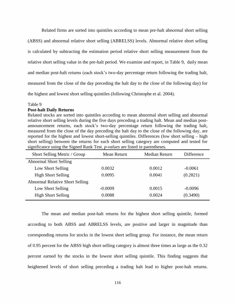
116
Related firms are sorted into quintiles according to mean pre-halt abnormal short selling
(ABSS) and abnormal relative short selling (ABRELSS) levels. Abnormal relative short selling
is calculated by subtracting the estimation period relative short selling measurement from the
relative short selling value in the pre-halt period. We examine and report, in Table 9, daily mean
and median post-halt returns (each stock’s two-day percentage return following the trading halt,
measured from the close of the day preceding the halt day to the close of the following day) for
the highest and lowest short selling quintiles (following Christophe et al. 2004).
Table 9
Post-halt Daily Returns
Related stocks are sorted into quintiles according to mean abnormal short selling and abnormal
relative short selling levels during the five days preceding a trading halt. Mean and median post-
announcement returns, each stock’s two-day percentage return following the trading halt,
measured from the close of the day preceding the halt day to the close of the following day, are
reported for the highest and lowest short-selling quintiles. Differences (low short selling – high
short selling) between the returns for each short selling category are computed and tested for
significance using the Signed Rank Test. p-values are listed in parentheses.
Short Selling Metric / Group Mean Return Median Return Difference
Abnormal Short Selling
Low Short Selling 0.0032 0.0012 -0.0061
High Short Selling 0.0095 0.0041 (0.2821)
Abnormal Relative Short Selling
Low Short Selling -0.0009 0.0015 -0.0096
High Short Selling 0.0088 0.0024 (0.3490)
The mean and median post-halt returns for the highest short selling quintile, formed
according to both ABSS and ABRELSS levels, are positive and larger in magnitude than
corresponding returns for stocks in the lowest short selling group. For instance, the mean return
of 0.95 percent for the ABSS high short selling category is almost three times as large as the 0.32
percent earned by the stocks in the lowest short selling quintile. This finding suggests that
heightened levels of short selling preceding a trading halt lead to higher post-halt returns.
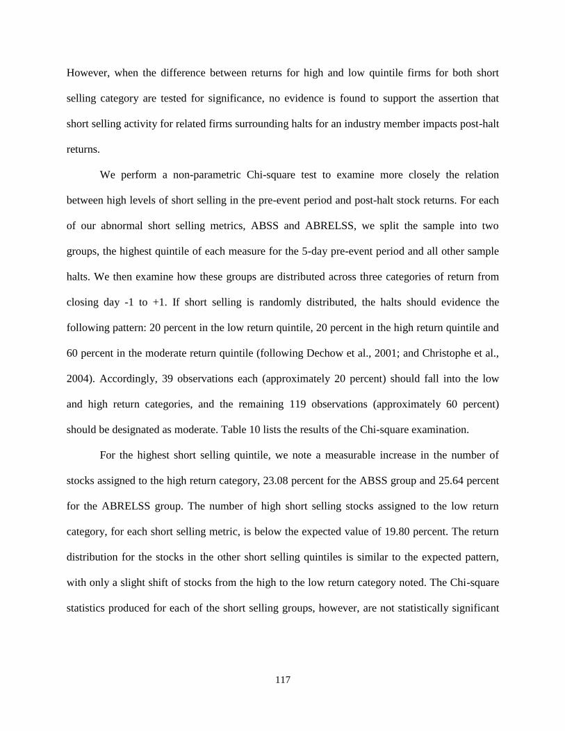
117
However, when the difference between returns for high and low quintile firms for both short
selling category are tested for significance, no evidence is found to support the assertion that
short selling activity for related firms surrounding halts for an industry member impacts post-halt
returns.
We perform a non-parametric Chi-square test to examine more closely the relation
between high levels of short selling in the pre-event period and post-halt stock returns. For each
of our abnormal short selling metrics, ABSS and ABRELSS, we split the sample into two
groups, the highest quintile of each measure for the 5-day pre-event period and all other sample
halts. We then examine how these groups are distributed across three categories of return from
closing day -1 to +1. If short selling is randomly distributed, the halts should evidence the
following pattern: 20 percent in the low return quintile, 20 percent in the high return quintile and
60 percent in the moderate return quintile (following Dechow et al., 2001; and Christophe et al.,
2004). Accordingly, 39 observations each (approximately 20 percent) should fall into the low
and high return categories, and the remaining 119 observations (approximately 60 percent)
should be designated as moderate. Table 10 lists the results of the Chi-square examination.
For the highest short selling quintile, we note a measurable increase in the number of
stocks assigned to the high return category, 23.08 percent for the ABSS group and 25.64 percent
for the ABRELSS group. The number of high short selling stocks assigned to the low return
category, for each short selling metric, is below the expected value of 19.80 percent. The return
distribution for the stocks in the other short selling quintiles is similar to the expected pattern,
with only a slight shift of stocks from the high to the low return category noted. The Chi-square
statistics produced for each of the short selling groups, however, are not statistically significant
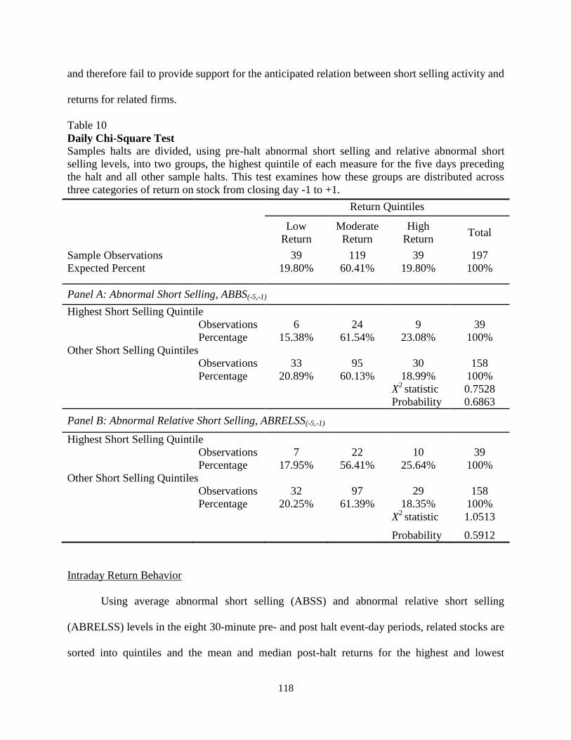
118
and therefore fail to provide support for the anticipated relation between short selling activity and
returns for related firms.
Table 10
Daily Chi-Square Test
Samples halts are divided, using pre-halt abnormal short selling and relative abnormal short
selling levels, into two groups, the highest quintile of each measure for the five days preceding
the halt and all other sample halts. This test examines how these groups are distributed across
three categories of return on stock from closing day -1 to +1.
Return Quintiles
Low
Return
Moderate
Return
High
Return Total
Sample Observations 39 119 39 197
Expected Percent 19.80% 60.41% 19.80% 100%
Panel A: Abnormal Short Selling, ABBS(-5,-1)
Highest Short Selling Quintile
Observations 6 24 9 39
Percentage 15.38% 61.54% 23.08% 100%
Other Short Selling Quintiles
Observations 33 95 30 158
Percentage 20.89% 60.13% 18.99% 100%
X2
statistic 0.7528
Probability 0.6863
Panel B: Abnormal Relative Short Selling, ABRELSS(-5,-1)
Highest Short Selling Quintile
Observations 7 22 10 39
Percentage 17.95% 56.41% 25.64% 100%
Other Short Selling Quintiles
Observations 32 97 29 158
Percentage 20.25% 61.39% 18.35% 100%
X2
statistic 1.0513
Probability 0.5912
Intraday Return Behavior
Using average abnormal short selling (ABSS) and abnormal relative short selling
(ABRELSS) levels in the eight 30-minute pre- and post halt event-day periods, related stocks are
sorted into quintiles and the mean and median post-halt returns for the highest and lowest
119
quintiles are examined (Christophe et al. 2004). We calculate three different intraday returns: 1)
from the close of the period preceding the halt to the reopen, 2) from the reopen to the close of
the period following resumption of trading, and 3) the interval spanning the halt, from the close
of the period prior to the halt to the close of the period following the halt. Return values are
reported only for stocks in the lowest and highest short selling quintiles.
Results, listed in Table 11, show that returns for the highest short selling quintile in each
period, with the exception of ABRELSS return1, are positive. For the stocks with the highest
levels of short selling, each return is larger than the corresponding return for stocks in the lowest
short selling quintile. For each short selling metric, differences between returns for the low and
high short quintiles is calculated and tested for significance. None of the difference values are
statistically different from zero - these results fail to provide support for our hypothesis that for
informationally related stocks, increased short selling activity surrounding interruptions in
trading is associated with negative price movements.
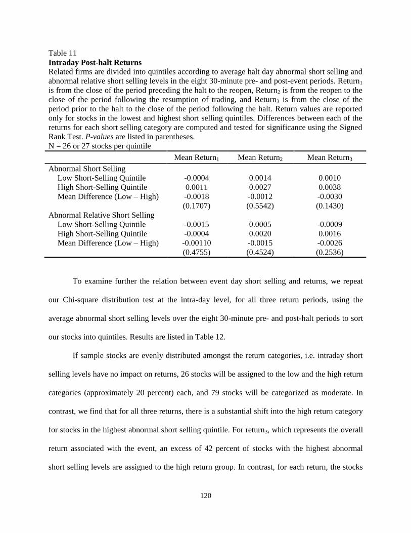
120
Table 11
Intraday Post-halt Returns
Related firms are divided into quintiles according to average halt day abnormal short selling and
abnormal relative short selling levels in the eight 30-minute pre- and post-event periods. Return1
is from the close of the period preceding the halt to the reopen, Return2 is from the reopen to the
close of the period following the resumption of trading, and Return3 is from the close of the
period prior to the halt to the close of the period following the halt. Return values are reported
only for stocks in the lowest and highest short selling quintiles. Differences between each of the
returns for each short selling category are computed and tested for significance using the Signed
Rank Test. P-values are listed in parentheses.
N = 26 or 27 stocks per quintile
Mean Return1 Mean Return2 Mean Return3
Abnormal Short Selling
Low Short-Selling Quintile -0.0004 0.0014 0.0010
High Short-Selling Quintile 0.0011 0.0027 0.0038
Mean Difference (Low – High) -0.0018
(0.1707)
-0.0012
(0.5542)
-0.0030
(0.1430)
Abnormal Relative Short Selling
Low Short-Selling Quintile -0.0015 0.0005 -0.0009
High Short-Selling Quintile -0.0004 0.0020 0.0016
Mean Difference (Low – High) -0.00110
(0.4755)
-0.0015
(0.4524)
-0.0026
(0.2536)
To examine further the relation between event day short selling and returns, we repeat
our Chi-square distribution test at the intra-day level, for all three return periods, using the
average abnormal short selling levels over the eight 30-minute pre- and post-halt periods to sort
our stocks into quintiles. Results are listed in Table 12.
If sample stocks are evenly distributed amongst the return categories, i.e. intraday short
selling levels have no impact on returns, 26 stocks will be assigned to the low and the high return
categories (approximately 20 percent) each, and 79 stocks will be categorized as moderate. In
contrast, we find that for all three returns, there is a substantial shift into the high return category
for stocks in the highest abnormal short selling quintile. For return3, which represents the overall
return associated with the event, an excess of 42 percent of stocks with the highest abnormal
short selling levels are assigned to the high return group. In contrast, for each return, the stocks
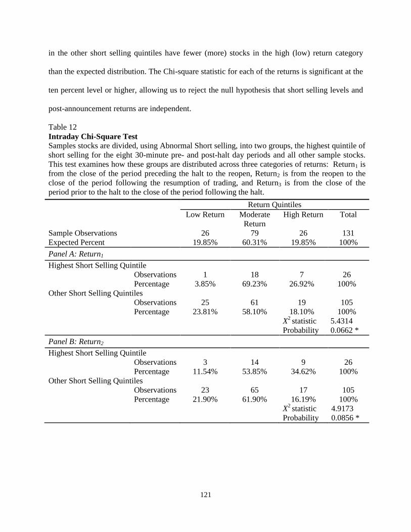
121
in the other short selling quintiles have fewer (more) stocks in the high (low) return category
than the expected distribution. The Chi-square statistic for each of the returns is significant at the
ten percent level or higher, allowing us to reject the null hypothesis that short selling levels and
post-announcement returns are independent.
Table 12
Intraday Chi-Square Test
Samples stocks are divided, using Abnormal Short selling, into two groups, the highest quintile of
short selling for the eight 30-minute pre- and post-halt day periods and all other sample stocks.
This test examines how these groups are distributed across three categories of returns: Return1 is
from the close of the period preceding the halt to the reopen, Return2 is from the reopen to the
close of the period following the resumption of trading, and Return3 is from the close of the
period prior to the halt to the close of the period following the halt.
Return Quintiles
Low Return Moderate
Return
High Return Total
Sample Observations 26 79 26 131
Expected Percent 19.85% 60.31% 19.85% 100%
Panel A: Return1
Highest Short Selling Quintile
Observations 1 18 7 26
Percentage 3.85% 69.23% 26.92% 100%
Other Short Selling Quintiles
Observations 25 61 19 105
Percentage 23.81% 58.10% 18.10% 100%
X2
statistic 5.4314
Probability 0.0662 *
Panel B: Return2
Highest Short Selling Quintile
Observations 3 14 9 26
Percentage 11.54% 53.85% 34.62% 100%
Other Short Selling Quintiles
Observations 23 65 17 105
Percentage 21.90% 61.90% 16.19% 100%
X2
statistic 4.9173
Probability 0.0856 *
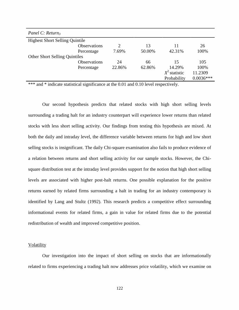
122
Panel C: Return3
Highest Short Selling Quintile
Observations 2 13 11 26
Percentage 7.69% 50.00% 42.31% 100%
Other Short Selling Quintiles
Observations 24 66 15 105
Percentage 22.86% 62.86% 14.29% 100%
X2
statistic 11.2309
Probability 0.0036***
*** and * indicate statistical significance at the 0.01 and 0.10 level respectively.
Our second hypothesis predicts that related stocks with high short selling levels
surrounding a trading halt for an industry counterpart will experience lower returns than related
stocks with less short selling activity. Our findings from testing this hypothesis are mixed. At
both the daily and intraday level, the difference variable between returns for high and low short
selling stocks is insignificant. The daily Chi-square examination also fails to produce evidence of
a relation between returns and short selling activity for our sample stocks. However, the Chi-
square distribution test at the intraday level provides support for the notion that high short selling
levels are associated with higher post-halt returns. One possible explanation for the positive
returns earned by related firms surrounding a halt in trading for an industry contemporary is
identified by Lang and Stultz (1992). This research predicts a competitive effect surrounding
informational events for related firms, a gain in value for related firms due to the potential
redistribution of wealth and improved competitive position.
Volatility
Our investigation into the impact of short selling on stocks that are informationally
related to firms experiencing a trading halt now addresses price volatility, which we examine on

123
both the daily and intraday level. Our hypothesis concerning the effect of short selling on price
volatility for our sample of related stocks states:
H3: Securities that are informationally related to a halted stock and have high short selling
levels will have higher price volatility surrounding trading halts as compared to
informationally related securities with lower short selling activity.
We calculate daily volatility measures for our related stocks for the pre-halt period, the
halt day, and the post-halt period following the methodology of Diether et al. (2009A). CRSP
data is used to compute a daily mean transaction price range [(high price – low price)/ high
price] and close-to-close volatility (by squaring the absolute daily return). The daily quote range
[(high quote – low quote) / high quote] and close-to-close and open-to-close volatility, using
absolute squared return, is calculated using TAQ data. We regress each volatility metric on a
post-halt dummy variable (which equals one for observations during the five-day post-halt
period); the coefficient obtained represents the difference between the pre- and post-halt
volatility measurements. The difference is tested, using the Wilcoxon signed-rank test, to
determine if it is significantly different from zero. We repeat each test, after dividing our sample
of related firms into quintiles according to levels of abnormal short selling in the eight 30-minute
pre- and post-halt intraday periods. Results are reported in Table 13 – Panel A and Panel B for
CRSP and TAQ data, respectively.
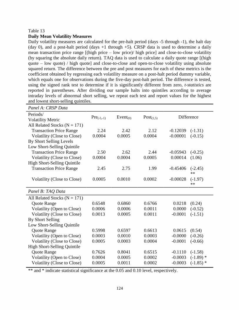
124
Table 13
Daily Mean Volatility Measures
Daily volatility measures are calculated for the pre-halt period (days -5 through -1), the halt day
(day 0), and a post-halt period (days +1 through +5). CRSP data is used to determine a daily
mean transaction price range [(high price – low price)/ high price] and close-to-close volatility
(by squaring the absolute daily return). TAQ data is used to calculate a daily quote range [(high
quote – low quote) / high quote] and close-to-close and open-to-close volatility using absolute
squared return. The difference between the pre and post measures for each of these metrics is the
coefficient obtained by regressing each volatility measure on a post-halt period dummy variable,
which equals one for observations during the five-day post-halt period. The difference is tested,
using the signed rank test to determine if it is significantly different from zero, t-statistics are
reported in parentheses. After dividing our sample halts into quintiles according to average
intraday levels of abnormal short selling, we repeat each test and report values for the highest
and lowest short-selling quintiles.
Panel A: CRSP Data
Periods/
Volatility Metric Pre(-5,-1) Event(0) Post(1,5) Difference
All Related Stocks (N = 171)
Transaction Price Range 2.24 2.42 2.12 -0.12039 (-1.31)
Volatility (Close to Close) 0.0004 0.0005 0.0004 -0.00001 (-0.15)
By Short Selling Levels
Low Short-Selling Quintile
Transaction Price Range 2.50 2.62 2.44 -0.05943 (-0.25)
Volatility (Close to Close) 0.0004 0.0004 0.0005 0.00014 (1.06)
High Short-Selling Quintile
Transaction Price Range 2.45 2.75 1.99 -0.45406 (-2.45)
**
Volatility (Close to Close) 0.0005 0.0010 0.0002 -0.00028 (-1.97)
**
Panel B: TAQ Data
All Related Stocks (N = 171)
Quote Range 0.6548 0.6860 0.6766 0.0218 (0.24)
Volatility (Open to Close) 0.0006 0.0006 0.0011 0.0000 (-0.52)
Volatility (Close to Close) 0.0013 0.0005 0.0011 -0.0001 (-1.51)
By Short Selling
Low Short-Selling Quintile
Quote Range 0.5998 0.6597 0.6613 0.0615 (0.54)
Volatility (Open to Close) 0.0003 0.0010 0.0003 -0.0000 (-0.26)
Volatility (Close to Close) 0.0005 0.0003 0.0004 -0.0001 (-0.66)
High Short-Selling Quintile
Quote Range 0.7626 0.8041 0.6515 -0.1110 (-1.58)
Volatility (Open to Close) 0.0004 0.0005 0.0002 -0.0003 (-1.89) *
Volatility (Close to Close) 0.0005 0.0011 0.0002 -0.0003 (-1.85) *
** and * indicate statistical significance at the 0.05 and 0.10 level, respectively.
125
Volatility metrics based on CRSP data demonstrate that the transaction price range for
sample stocks is larger on the event day as compared to the average price range in the pre- and
post-halt intervals. With the exception of the high short selling quintile, the event-day price range
is 18 to 30 percent larger than price ranges during the 5-day periods preceding and following the
halt day. The close-to-close volatility measurement for the all stocks and the low short selling
categories are nearly identical for the three examination periods, varying by only 0.0001.
Volatility measurements for the high short selling group demonstrate the largest amount of
variation. For this category, the halt day transaction price range is 30 percent greater than the
pre-halt value and 76 percent larger than the average price range in the post-halt period. Close-
to-close volatility increases by a factor of two (five) over pre-halt (post-halt) levels. For the high
short selling quintile, the difference value, comparing pre- and post-halt volatility measurements,
are negative for both the transaction price range and close-to-close volatility, indicating a
significant decrease in volatility for these related firms on the five trading days following a
trading halt event. Differences for the all stocks and low short selling quintile are not significant.
These results suggest that increased short selling activity for firms related to an industry member
experiencing a trading halt results in lower post-halt volatility.
The daily quote range and volatility metrics calculated with TAQ data provide similar
findings. Modest changes in the quote range are noted for the all stocks and the low short selling
quintile. However, close-to-close and open-to-close volatility appears elevated for all stocks in
the post-halt period and the event-day open-to-close volatility for stocks in the low short selling
category. None of the difference variables for the all sample stocks category and the quintile of
low short selling stocks are significant. In contrast, the high short selling quintile of stocks has
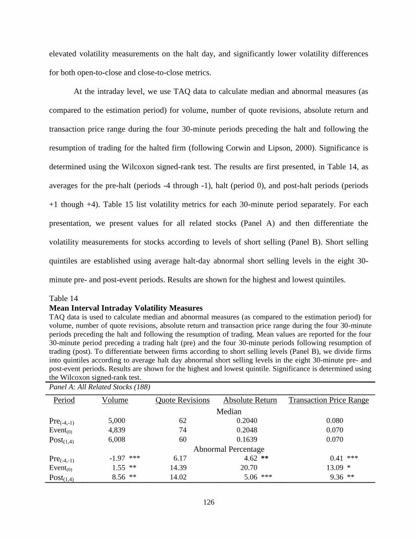
126
elevated volatility measurements on the halt day, and significantly lower volatility differences
for both open-to-close and close-to-close metrics.
At the intraday level, we use TAQ data to calculate median and abnormal measures (as
compared to the estimation period) for volume, number of quote revisions, absolute return and
transaction price range during the four 30-minute periods preceding the halt and following the
resumption of trading for the halted firm (following Corwin and Lipson, 2000). Significance is
determined using the Wilcoxon signed-rank test. The results are first presented, in Table 14, as
averages for the pre-halt (periods -4 through -1), halt (period 0), and post-halt periods (periods
+1 though +4). Table 15 list volatility metrics for each 30-minute period separately. For each
presentation, we present values for all related stocks (Panel A) and then differentiate the
volatility measurements for stocks according to levels of short selling (Panel B). Short selling
quintiles are established using average halt-day abnormal short selling levels in the eight 30-
minute pre- and post-event periods. Results are shown for the highest and lowest quintiles.
Table 14
Mean Interval Intraday Volatility Measures TAQ data is used to calculate median and abnormal measures (as compared to the estimation period) for
volume, number of quote revisions, absolute return and transaction price range during the four 30-minute
periods preceding the halt and following the resumption of trading. Mean values are reported for the four
30-minute period preceding a trading halt (pre) and the four 30-minute periods following resumption of
trading (post). To differentiate between firms according to short selling levels (Panel B), we divide firms
into quintiles according to average halt day abnormal short selling levels in the eight 30-minute pre- and
post-event periods. Results are shown for the highest and lowest quintile. Significance is determined using
the Wilcoxon signed-rank test.
Panel A: All Related Stocks (188)
Period Volume Quote Revisions Absolute Return Transaction Price Range
Median
Pre(-4,-1) 5,000 62 0.2040 0.080 Event(0) 4,839 74 0.2048 0.070
Post(1,4) 6,008 60 0.1639 0.070
Abnormal Percentage
Pre(-4,-1) -1.97 *** 6.17 4.62 ** 0.41 ***
Event(0) 1.55 ** 14.39 20.70 13.09 *
Post(1,4) 8.56 ** 14.02 5.06 *** 9.36 **

127
Panel B By short-selling levels (38 Halts per Quintile)
Lowest Short-selling Quintile
Median
Pre(-4,-1) 3,050 55 0.1640 0.055 Event(0) 3,429 78 0.1920 0.060
Post(1,4) 2,872 71 0.1524 0.040
Abnormal Percentage
Pre(-4,-1) -21.16 *** 5.70 * -15.23 *** -6.70 **
Event(0) -12.55 ** -3.57 32.50 -17.16
Post(1,4) -33.41 *** 15.73 -9.95 ** -21.94 ***
Highest Short-selling Quintile
Median
Pre(-4,-1) 12,300 73 0.2536 0.110 Event(0) 8,219 94 0.1221 0.070
Post(1,4) 10,116 82 0.2189 0.095
Abnormal Percentage
Pre(-4,-1) 53.30 *** 22.66 ** 16.06 6.98
Event(0) 47.80 * 34.52 -19.70 ** -5.79
Post(1,4) 75.31 *** 36.19 *** 28.26 35.87 **
*** and ** indicate statistical significance at the 0.01 and 0.05 level respectively.
Abnormal trading volume, for all stocks, is significantly different from trading volume in
the estimation period - levels are lower than normal (negative) preceding the halt and above
estimation period levels (positive) during and following the halt period. Our examination of
abnormal volume for each of our short selling quintiles demonstrates that abnormal trading
volume is negative (12 to 33 percent lower) for stocks in the low short selling quintile. For stocks
in the high short selling category, median period values are substantially larger and abnormal
volume is positive (47 to 75 percent) in each of the periods examined. This finding suggests that
short selling has a positive relation with trading volume and subsequent volatility.
For the all stocks category, the number of quote revisions is not statistically different
from the level generated during the estimation period. However, when segmented according to
short selling levels, stocks in the low short selling group demonstrate a higher than normal
number of quote revisions in the pre-halt period. Stocks with the highest level of short selling
128
appear to have an increased number and significantly elevated abnormal quote revisions in both
the pre- and post-halt periods.
Increased volatility, in the form of absolute returns, is noted for all stocks in the pre- and
post-halt periods. However, when examining this metric for stocks segmented by shorting
activity, both quintiles experience negative abnormal absolute returns, stocks with low levels of
shorting during the pre- and post-halt periods, and stocks in the high short selling quintile during
the halt interval.
The transaction price range is larger than estimation period levels for all stocks in the pre,
halt, and post–halt periods. This positive relation is also evident during the post-halt period for
stocks with the highest level of short selling. In contrast, stocks with low shorting levels
demonstrate a substantially lower price range immediately preceding and following the halt in
trading for an industry member.
Table 15 presents the volatility metrics for each period separately (Panel A) and then
separates firms according to short selling levels (Panel B). For all related firms, abnormal
volume is negative in periods -4 and -3; this metric is positive in the two periods immediately
preceding the halt and the during the halt period. Although median values appear larger in the
four post-halt periods, there is no statistical difference between halt and estimation period levels
for these intervals. When segmented according to levels of short selling, a general pattern
emerges; stocks with the lowest (highest) levels of short selling demonstrate negative (positive)
abnormal volume.
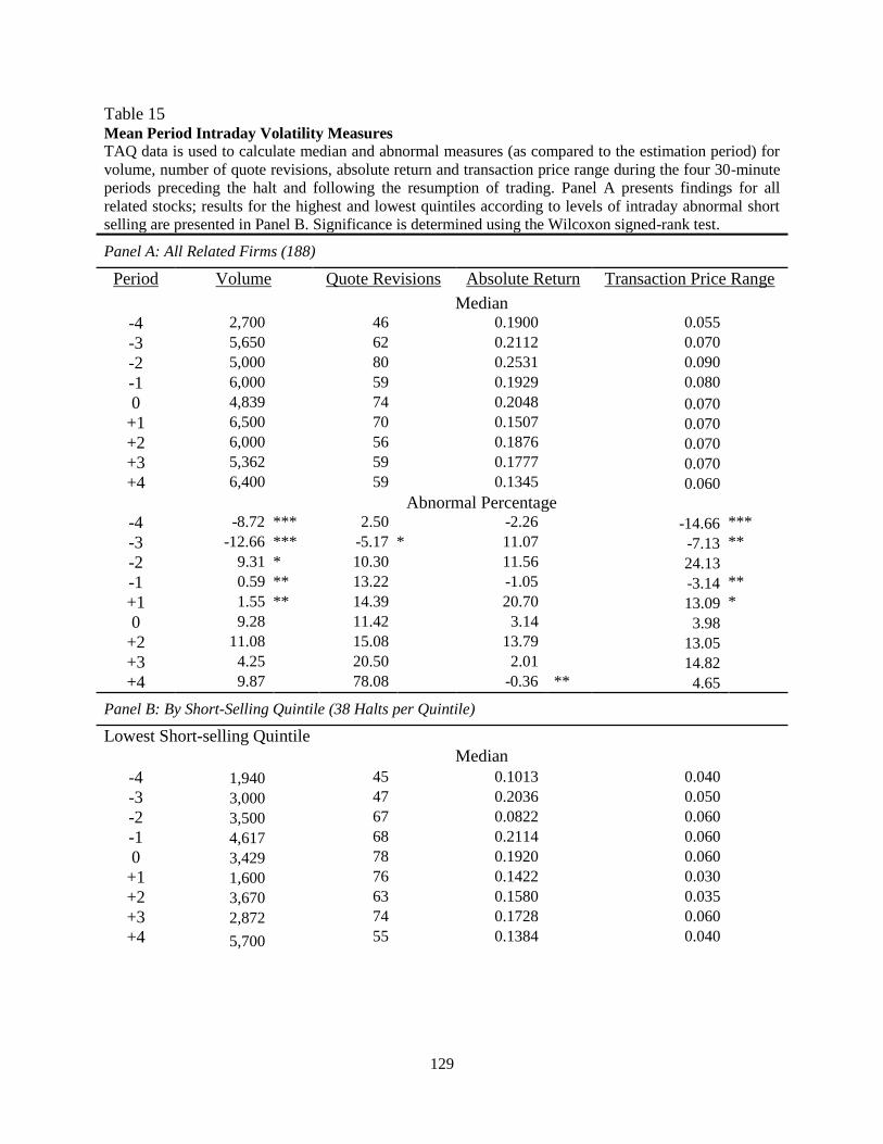
129
Table 15 Mean Period Intraday Volatility Measures
TAQ data is used to calculate median and abnormal measures (as compared to the estimation period) for
volume, number of quote revisions, absolute return and transaction price range during the four 30-minute
periods preceding the halt and following the resumption of trading. Panel A presents findings for all
related stocks; results for the highest and lowest quintiles according to levels of intraday abnormal short
selling are presented in Panel B. Significance is determined using the Wilcoxon signed-rank test.
Panel A: All Related Firms (188)
Period Volume Quote Revisions Absolute Return Transaction Price Range
Median
-4 2,700 46 0.1900 0.055
-3 5,650 62 0.2112 0.070
-2 5,000 80 0.2531 0.090
-1 6,000 59 0.1929 0.080
0 4,839 74 0.2048 0.070
+1 6,500 70 0.1507 0.070
+2 6,000 56 0.1876 0.070
+3 5,362 59 0.1777 0.070
+4 6,400 59 0.1345 0.060
Abnormal Percentage
-4 -8.72 *** 2.50 -2.26 -14.66 ***
-3 -12.66 *** -5.17 * 11.07 -7.13 **
-2 9.31 * 10.30 11.56 24.13
-1 0.59 ** 13.22 -1.05 -3.14 **
+1 1.55 ** 14.39 20.70 13.09 *
0 9.28 11.42 3.14 3.98
+2 11.08 15.08 13.79 13.05
+3 4.25 20.50 2.01 14.82
+4 9.87 78.08 -0.36 ** 4.65
Panel B: By Short-Selling Quintile (38 Halts per Quintile)
Lowest Short-selling Quintile
Median
-4 1,940 45 0.1013 0.040
-3 3,000 47 0.2036 0.050
-2 3,500 67 0.0822 0.060
-1 4,617 68 0.2114 0.060
0 3,429 78 0.1920 0.060
+1 1,600 76 0.1422 0.030
+2 3,670 63 0.1580 0.035
+3 2,872 74 0.1728 0.060
+4 5,700 55 0.1384 0.040
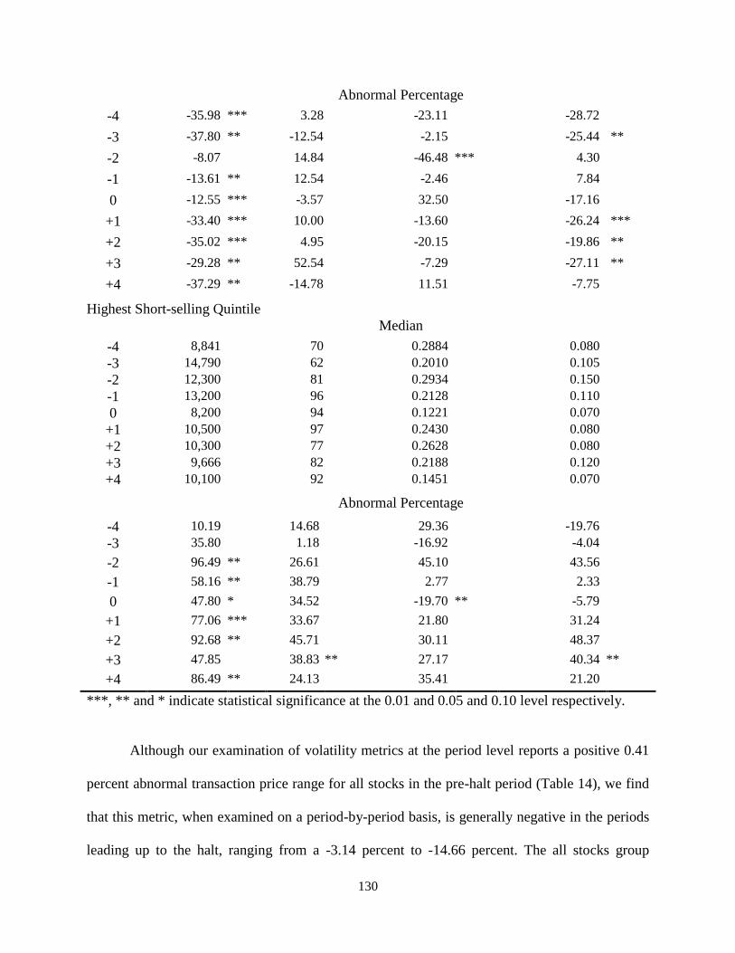
130
Abnormal Percentage
-4 -35.98 *** 3.28 -23.11 -28.72
-3 -37.80 ** -12.54 -2.15 -25.44 **
-2 -8.07 14.84 -46.48 *** 4.30
-1 -13.61 ** 12.54 -2.46 7.84
0 -12.55 *** -3.57 32.50 -17.16
+1 -33.40 *** 10.00 -13.60 -26.24 ***
+2 -35.02 *** 4.95 -20.15 -19.86 **
+3 -29.28 ** 52.54 -7.29 -27.11 **
+4 -37.29 ** -14.78 11.51 -7.75
Highest Short-selling Quintile
Median
-4 8,841 70 0.2884 0.080
-3 14,790 62 0.2010 0.105
-2 12,300 81 0.2934 0.150
-1 13,200 96 0.2128 0.110
0 8,200 94 0.1221 0.070
+1 10,500 97 0.2430 0.080
+2 10,300 77 0.2628 0.080
+3 9,666 82 0.2188 0.120
+4 10,100 92 0.1451 0.070
Abnormal Percentage
-4 10.19 14.68 29.36 -19.76
-3 35.80 1.18 -16.92 -4.04
-2 96.49 ** 26.61 45.10 43.56
-1 58.16 ** 38.79 2.77 2.33
0 47.80 * 34.52 -19.70 ** -5.79
+1 77.06 *** 33.67 21.80 31.24
+2 92.68 ** 45.71 30.11 48.37
+3 47.85 38.83 ** 27.17 40.34 **
+4 86.49 ** 24.13 35.41 21.20
***, ** and * indicate statistical significance at the 0.01 and 0.05 and 0.10 level respectively.
Although our examination of volatility metrics at the period level reports a positive 0.41
percent abnormal transaction price range for all stocks in the pre-halt period (Table 14), we find
that this metric, when examined on a period-by-period basis, is generally negative in the periods
leading up to the halt, ranging from a -3.14 percent to -14.66 percent. The all stocks group

131
reports a positive 9.36 percent abnormal price range in the post-halt period, yet a significant
increase in abnormal price range is not supported when reporting by periods - the lowest short
selling quintile demonstrates negative abnormal transaction price ranges following the
resumption in trading for the halted firm (periods +1 through +3).
Based on the findings of previous literature, we hypothesize that short selling activity has
a positive impact on volatility for stocks related to an industry member experiencing a trading
halt. Our examination of volatility, however, provides mixed results. At the daily level, we find
evidence, in the form of a lower transaction price range and close-to-close and open-to-open
volatility measurements, those stocks with the highest short selling levels demonstrate lower
post-halt volatility – short selling appears to reduce these metrics in our sample of related stocks.
However, at the intraday level, our findings suggest that stocks with the lowest level of short
selling activity have reduced volatility (negative abnormal volume and abnormal transaction
price range) as compared to stocks with higher short selling (positive abnormal volume).
Spreads
Previous research has established that short selling and trading halts both impact the bid-
ask spread. To investigate the combined effect of these two market activities, we examine mean
and median dollar spreads for related firms at several intervals preceding the halt period and
following the resumption of trading for the halted firm.
Our hypothesis concerning the effect of short selling activity on spreads surrounding
interruptions in trading purports:
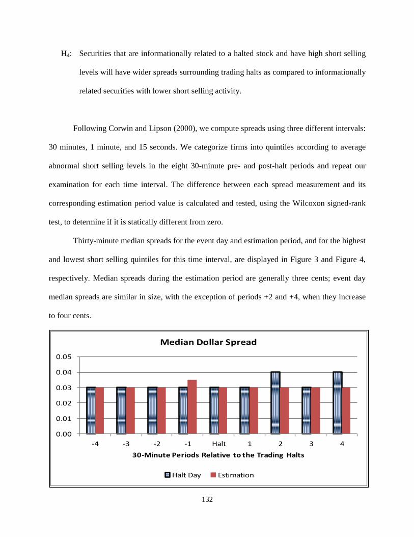
132
H4: Securities that are informationally related to a halted stock and have high short selling
levels will have wider spreads surrounding trading halts as compared to informationally
related securities with lower short selling activity.
Following Corwin and Lipson (2000), we compute spreads using three different intervals:
30 minutes, 1 minute, and 15 seconds. We categorize firms into quintiles according to average
abnormal short selling levels in the eight 30-minute pre- and post-halt periods and repeat our
examination for each time interval. The difference between each spread measurement and its
corresponding estimation period value is calculated and tested, using the Wilcoxon signed-rank
test, to determine if it is statically different from zero.
Thirty-minute median spreads for the event day and estimation period, and for the highest
and lowest short selling quintiles for this time interval, are displayed in Figure 3 and Figure 4,
respectively. Median spreads during the estimation period are generally three cents; event day
median spreads are similar in size, with the exception of periods +2 and +4, when they increase
to four cents.
0.00
0.01
0.02
0.03
0.04
0.05
-4 -3 -2 -1 Halt 1 2 3 4
30-Minute Periods Relative to the Trading Halts
Median Dollar Spread
Halt Day Estimation
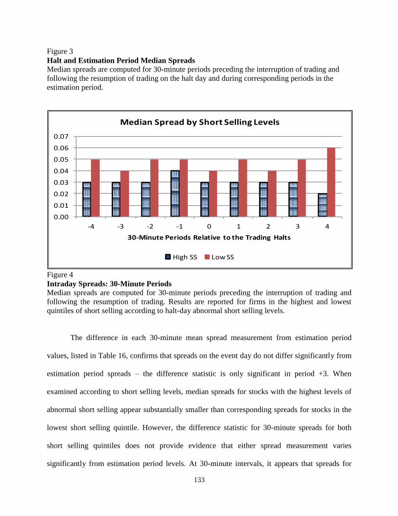
133
Figure 3
Halt and Estimation Period Median Spreads
Median spreads are computed for 30-minute periods preceding the interruption of trading and
following the resumption of trading on the halt day and during corresponding periods in the
estimation period.
Figure 4
Intraday Spreads: 30-Minute Periods
Median spreads are computed for 30-minute periods preceding the interruption of trading and
following the resumption of trading. Results are reported for firms in the highest and lowest
quintiles of short selling according to halt-day abnormal short selling levels.
The difference in each 30-minute mean spread measurement from estimation period
values, listed in Table 16, confirms that spreads on the event day do not differ significantly from
estimation period spreads – the difference statistic is only significant in period +3. When
examined according to short selling levels, median spreads for stocks with the highest levels of
abnormal short selling appear substantially smaller than corresponding spreads for stocks in the
lowest short selling quintile. However, the difference statistic for 30-minute spreads for both
short selling quintiles does not provide evidence that either spread measurement varies
significantly from estimation period levels. At 30-minute intervals, it appears that spreads for
0.00
0.01
0.02
0.03
0.04
0.05
0.06
0.07
-4 -3 -2 -1 0 1 2 3 4
30-Minute Periods Relative to the Trading Halts
Median Spread by Short Selling Levels
High SS Low SS
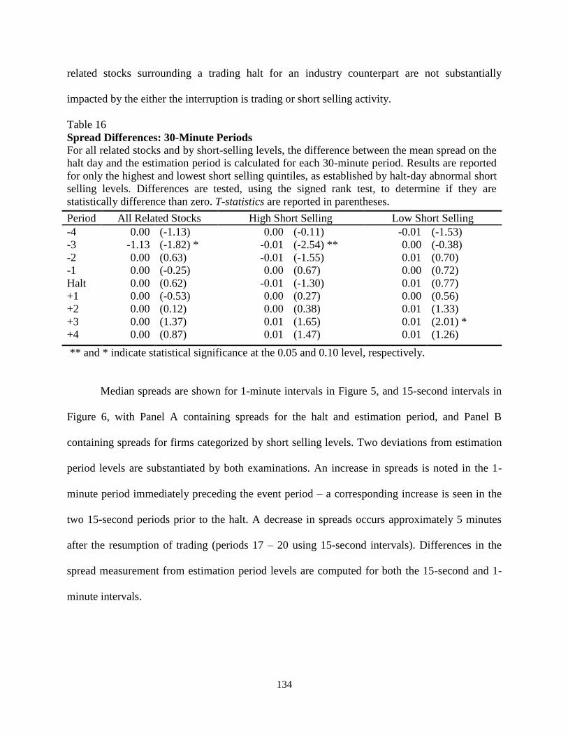
134
related stocks surrounding a trading halt for an industry counterpart are not substantially
impacted by the either the interruption is trading or short selling activity.
Table 16
Spread Differences: 30-Minute Periods
For all related stocks and by short-selling levels, the difference between the mean spread on the
halt day and the estimation period is calculated for each 30-minute period. Results are reported
for only the highest and lowest short selling quintiles, as established by halt-day abnormal short
selling levels. Differences are tested, using the signed rank test, to determine if they are
statistically difference than zero. T-statistics are reported in parentheses.
Period All Related Stocks High Short Selling Low Short Selling
-4 0.00 (-1.13) 0.00 (-0.11) -0.01 (-1.53)
-3 -1.13 (-1.82) * -0.01 (-2.54) ** 0.00 (-0.38)
-2 0.00 (0.63) -0.01 (-1.55) 0.01 (0.70)
-1 0.00 (-0.25) 0.00 (0.67) 0.00 (0.72)
Halt 0.00 (0.62) -0.01 (-1.30) 0.01 (0.77)
+1 0.00 (-0.53) 0.00 (0.27) 0.00 (0.56)
+2 0.00 (0.12) 0.00 (0.38) 0.01 (1.33)
+3 0.00 (1.37) 0.01 (1.65) 0.01 (2.01) *
+4 0.00 (0.87) 0.01 (1.47) 0.01 (1.26)
** and * indicate statistical significance at the 0.05 and 0.10 level, respectively.
Median spreads are shown for 1-minute intervals in Figure 5, and 15-second intervals in
Figure 6, with Panel A containing spreads for the halt and estimation period, and Panel B
containing spreads for firms categorized by short selling levels. Two deviations from estimation
period levels are substantiated by both examinations. An increase in spreads is noted in the 1-
minute period immediately preceding the event period – a corresponding increase is seen in the
two 15-second periods prior to the halt. A decrease in spreads occurs approximately 5 minutes
after the resumption of trading (periods 17 – 20 using 15-second intervals). Differences in the
spread measurement from estimation period levels are computed for both the 15-second and 1-
minute intervals.
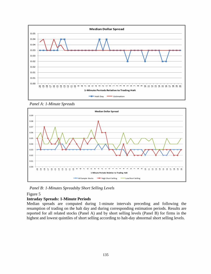
135
Panel A: 1-Minute Spreads
Panel B: 1-Minutes Spreadsby Short Selling Levels
Figure 5
Intraday Spreads: 1-Minute Periods
Median spreads are computed during 1-minute intervals preceding and following the
resumption of trading on the halt day and during corresponding estimation periods. Results are
reported for all related stocks (Panel A) and by short selling levels (Panel B) for firms in the
highest and lowest quintiles of short selling according to halt-day abnormal short selling levels.
0.00
0.01
0.01
0.02
0.02
0.03
0.03
0.04
0.04
0.05
-20
-19
-18
-17
-16
-15
-14
-13
-12
-11
-10 -9 -8 -7 -6 -5 -4 -3 -2 -1 0 1 2 3 4 5 6 7 8 9 10 11 12 13 14 15 16 17 18 19 20
1-Minute Periods Relative to Trading Halt
Median Dollar Spread
Halt Day Estimation
0.00
0.01
0.02
0.03
0.04
0.05
0.06
0.07
0.08
0.09
-20
-19
-18
-17
-16
-15
-14
-13
-12
-11
-10 -9 -8 -7 -6 -5 -4 -3 -2 -1 0 1 2 3 4 5 6 7 8 9
10
11
12
13
14
15
16
17
18
19
20
1-Minute Periods Relative to Trading Halt
Median Dollar Spread
All Sample Stocks High Short Selling Low Short Selling
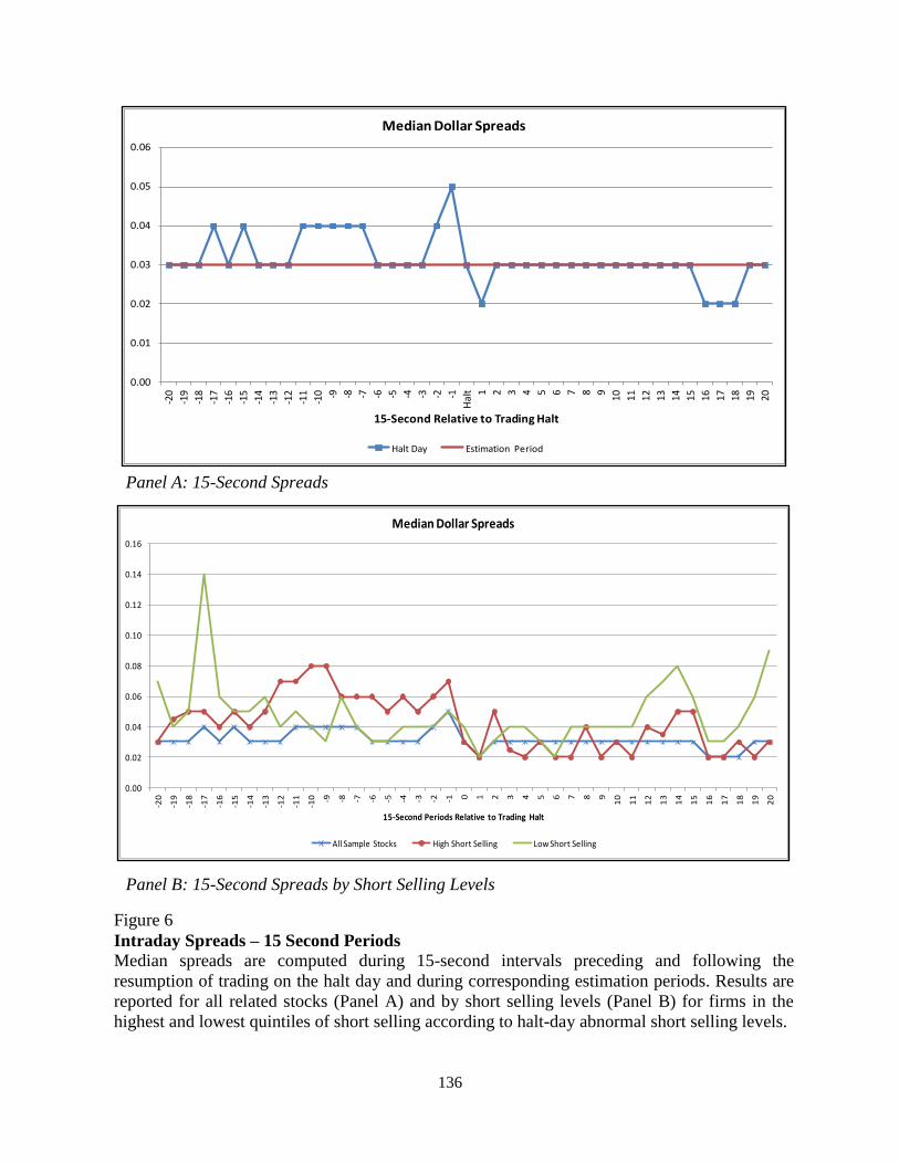
136
Panel A: 15-Second Spreads
Panel B: 15-Second Spreads by Short Selling Levels
Figure 6
Intraday Spreads – 15 Second Periods
Median spreads are computed during 15-second intervals preceding and following the
resumption of trading on the halt day and during corresponding estimation periods. Results are
reported for all related stocks (Panel A) and by short selling levels (Panel B) for firms in the
highest and lowest quintiles of short selling according to halt-day abnormal short selling levels.
0.00
0.01
0.02
0.03
0.04
0.05
0.06
-20
-19
-18
-17
-16
-15
-14
-13
-12
-11
-10 -9 -8 -7 -6 -5 -4 -3 -2 -1
Hal
t 1 2 3 4 5 6 7 8 9
10 11 12 13 14 15 16 17 18 19 20
15-Second Relative to Trading Halt
Median Dollar Spreads
Halt Day Estimation Period
0.00
0.02
0.04
0.06
0.08
0.10
0.12
0.14
0.16
-20
-19
-18
-17
-16
-15
-14
-13
-12
-11
-10 -9 -8 -7 -6 -5 -4 -3 -2 -1 0 1 2 3 4 5 6 7 8 9
10
11
12
13
14
15
16
17
18
19
20
15-Second Periods Relative to Trading Halt
Median Dollar Spreads
All Sample Stocks High Short Selling Low Short Selling
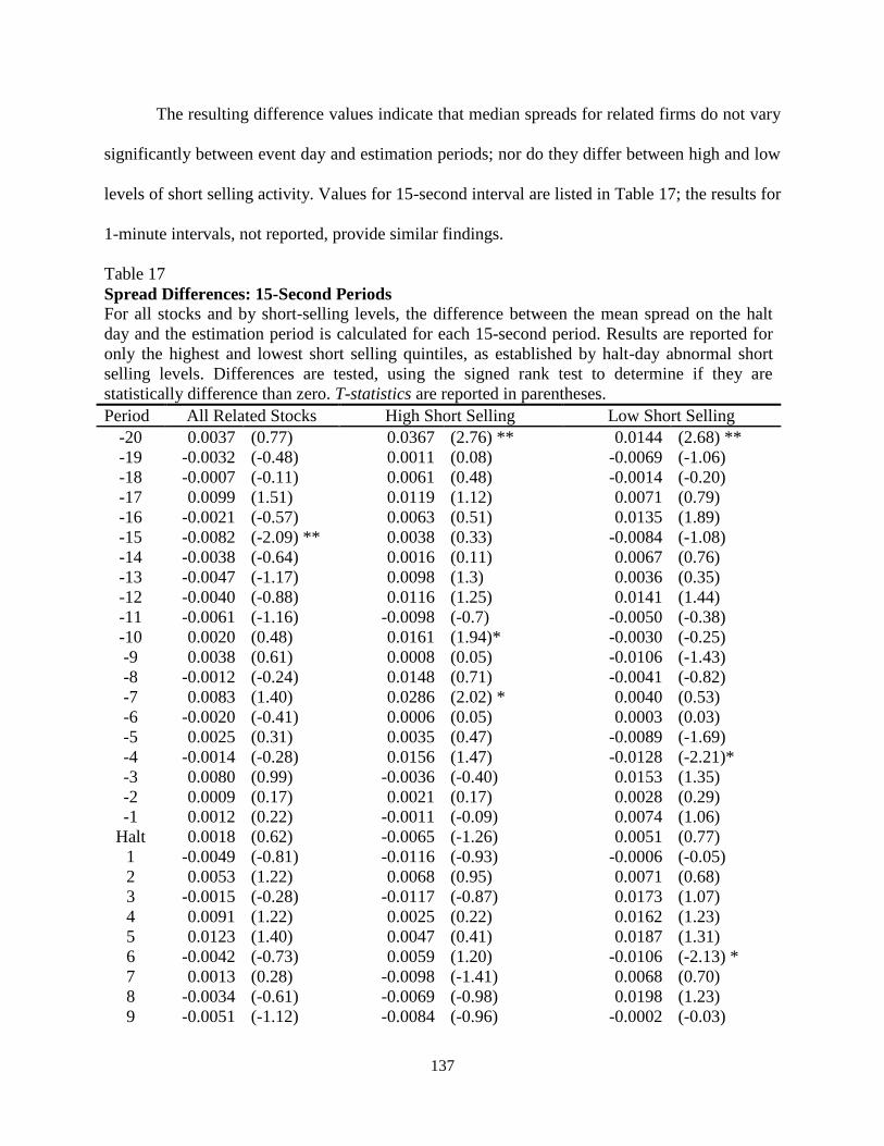
137
The resulting difference values indicate that median spreads for related firms do not vary
significantly between event day and estimation periods; nor do they differ between high and low
levels of short selling activity. Values for 15-second interval are listed in Table 17; the results for
1-minute intervals, not reported, provide similar findings.
Table 17
Spread Differences: 15-Second Periods
For all stocks and by short-selling levels, the difference between the mean spread on the halt
day and the estimation period is calculated for each 15-second period. Results are reported for
only the highest and lowest short selling quintiles, as established by halt-day abnormal short
selling levels. Differences are tested, using the signed rank test to determine if they are
statistically difference than zero. T-statistics are reported in parentheses.
Period All Related Stocks High Short Selling Low Short Selling
-20 0.0037 (0.77) 0.0367 (2.76) ** 0.0144 (2.68) **
-19 -0.0032 (-0.48) 0.0011 (0.08) -0.0069 (-1.06)
-18 -0.0007 (-0.11) 0.0061 (0.48) -0.0014 (-0.20)
-17 0.0099 (1.51) 0.0119 (1.12) 0.0071 (0.79)
-16 -0.0021 (-0.57) 0.0063 (0.51) 0.0135 (1.89)
-15 -0.0082 (-2.09) ** 0.0038 (0.33) -0.0084 (-1.08)
-14 -0.0038 (-0.64) 0.0016 (0.11) 0.0067 (0.76)
-13 -0.0047 (-1.17) 0.0098 (1.3) 0.0036 (0.35)
-12 -0.0040 (-0.88) 0.0116 (1.25) 0.0141 (1.44)
-11 -0.0061 (-1.16) -0.0098 (-0.7) -0.0050 (-0.38)
-10 0.0020 (0.48) 0.0161 (1.94)* -0.0030 (-0.25)
-9 0.0038 (0.61) 0.0008 (0.05) -0.0106 (-1.43)
-8 -0.0012 (-0.24) 0.0148 (0.71) -0.0041 (-0.82)
-7 0.0083 (1.40) 0.0286 (2.02) * 0.0040 (0.53)
-6 -0.0020 (-0.41) 0.0006 (0.05) 0.0003 (0.03)
-5 0.0025 (0.31) 0.0035 (0.47) -0.0089 (-1.69)
-4 -0.0014 (-0.28) 0.0156 (1.47) -0.0128 (-2.21)*
-3 0.0080 (0.99) -0.0036 (-0.40) 0.0153 (1.35)
-2 0.0009 (0.17) 0.0021 (0.17) 0.0028 (0.29)
-1 0.0012 (0.22) -0.0011 (-0.09) 0.0074 (1.06)
Halt 0.0018 (0.62) -0.0065 (-1.26) 0.0051 (0.77)
1 -0.0049 (-0.81) -0.0116 (-0.93) -0.0006 (-0.05)
2 0.0053 (1.22) 0.0068 (0.95) 0.0071 (0.68)
3 -0.0015 (-0.28) -0.0117 (-0.87) 0.0173 (1.07)
4 0.0091 (1.22) 0.0025 (0.22) 0.0162 (1.23)
5 0.0123 (1.40) 0.0047 (0.41) 0.0187 (1.31)
6 -0.0042 (-0.73) 0.0059 (1.20) -0.0106 (-2.13) *
7 0.0013 (0.28) -0.0098 (-1.41) 0.0068 (0.70)
8 -0.0034 (-0.61) -0.0069 (-0.98) 0.0198 (1.23)
9 -0.0051 (-1.12) -0.0084 (-0.96) -0.0002 (-0.03)
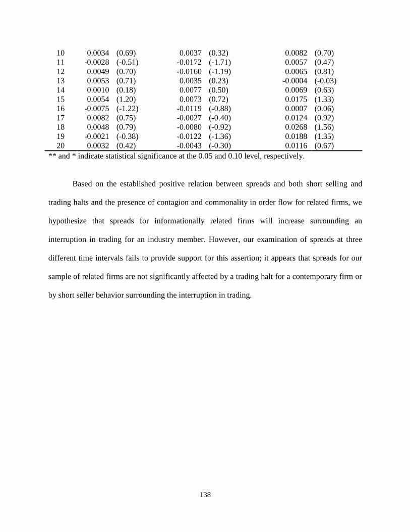
138
10 0.0034 (0.69) 0.0037 (0.32) 0.0082 (0.70)
11 -0.0028 (-0.51) -0.0172 (-1.71) 0.0057 (0.47)
12 0.0049 (0.70) -0.0160 (-1.19) 0.0065 (0.81)
13 0.0053 (0.71) 0.0035 (0.23) -0.0004 (-0.03)
14 0.0010 (0.18) 0.0077 (0.50) 0.0069 (0.63)
15 0.0054 (1.20) 0.0073 (0.72) 0.0175 (1.33)
16 -0.0075 (-1.22) -0.0119 (-0.88) 0.0007 (0.06)
17 0.0082 (0.75) -0.0027 (-0.40) 0.0124 (0.92)
18 0.0048 (0.79) -0.0080 (-0.92) 0.0268 (1.56)
19 -0.0021 (-0.38) -0.0122 (-1.36) 0.0188 (1.35)
20 0.0032 (0.42) -0.0043 (-0.30) 0.0116 (0.67)
** and * indicate statistical significance at the 0.05 and 0.10 level, respectively.
Based on the established positive relation between spreads and both short selling and
trading halts and the presence of contagion and commonality in order flow for related firms, we
hypothesize that spreads for informationally related firms will increase surrounding an
interruption in trading for an industry member. However, our examination of spreads at three
different time intervals fails to provide support for this assertion; it appears that spreads for our
sample of related firms are not significantly affected by a trading halt for a contemporary firm or
by short seller behavior surrounding the interruption in trading.
139
CONCLUSION
The objective of this research is to determine if informed market participants modify their
behavior, in regards to short selling activity, for stocks that are informationally related to
industry contemporaries that experience a halt in trading. Further, our aim is to discover if the
anticipated increase in short selling substantially affects market quality for these related firms.
Our investigation is based on the previously established impact of both short selling and trading
halts on security prices, return variability, and spreads, and the contagion and commonality in
order flow between industry counterparts identified in previous research.
Our results provide some evidence that short sellers modify their behavior in regards to
related firms surrounding halts in trading for an industry member. At the daily level, short sellers
appear to reduce their activity regarding related firms prior to and following a trading halt – they
submit fewer trades, resulting in a decrease in short volume during the 5-day pre- and post-halt
periods. A decrease is short selling activity is also detected at the intraday level, as the average
trade size, volume, short interest ratio, and abnormal short selling measures decrease prior to the
halt period. However, an increase in shorting is identified in the 30-minute period immediately
following the resumption of trading, as the average short trade size, volume, and abnormal short
selling levels are significantly above estimation period values. Although changes in short selling
activity were identified prior to the implementation of a halt, the lack of significance in our
regression equations do not provide the support necessary for us to purport that this activity is
informationally motivated.
140
Hypothesis 2 is based on the established relation between short selling and returns; it
suggests that an increase in short selling leads to negative returns for our sample of related
stocks. Although no significant findings were obtained from the daily examination, results from
the intraday Chi-square test suggests that related firms with the highest short selling levels earn
larger gains that sample firms with lower levels of short activity. One possible explanation for
this result is that related firms derive a benefit (i.e. the competitive effect suggested by Lang and
Stultz, 1992) when a fellow industry member is subjected to a halt in trading.
Our examination of volatility for related firms provides evidence that price volatility is
affected by the halt in trading for an industry member. Intraday results for volume, absolute
return, and transaction price ranges are generally higher surrounding halts in trading than during
the estimation period. Short selling levels appear to impact volatility; at the daily level short
selling activity appears to mitigate volatility, reducing the transaction price and quote range and
close-to-close and open-to-close volatility metrics. In the intraday periods immediately
surrounding the halt interval, however, firms with low short selling levels evidence lower
volume, absolute return, and transaction price range than corresponding estimation period levels.
In support of Hypothesis 3, stocks with the highest shorting activity demonstrate an increase in
volume and the number of quote revisions.
Our final hypothesis predicts that spreads will increase for related firms surrounding halts
in trading for an industry counterpart. This notion is based on the high levels of information
asymmetry associated with halts in trading and the corresponding need for wider spreads to
compensate for losses to informed traders. Our examination of spreads was unable to detect any
significant deviation from estimation periods or between stocks with different levels of short
selling activity.

141
This investigation into short selling activity for related firms surrounding halts in trading
for an industry member provides mixed results. Although a shift in short selling activity and a
modest impact in market quality is detected in our sample of related firms, our examination fails
to establish that these changes are informationally motivated.

142
LIST OF REFERENCES

143
Aharony, Joseph, and Itzhak Swary, 1980, Quarterly Dividend and Earnings Announcements and
Stockholders’ Returns: An Empirical Analysis, The Journal of Finance, 35 (1), 1 – 12.
Aitken, Michael, Alex Frino, Michael McCorry, and Peter Swan, 1998, Short Sales are Almost
Always Bad News: Evidence from the Australian Stock Exchange, The Journal of Finance,
53 (6), 2205 – 2223.
Alli, Kasim, Samantha Thapa, and Kenneth Yung, 1994, Stock Price Dynamics in Overlapped
Market Segments: Intra and Inter-Industry Contagion Effects, Journal of Business Finance
and Accounting, 21 (7), 1059 – 1070.
Angel, James, Stephen Christophe, and Michael Ferri, 2003, A Close Look at Short Selling on
Nasdaq, Financial Analyst Journal, 59 (6), 66 – 74.
Arnold, Tom, Alexander Butler, Timothy Crack and Yan Zhang, 2005, The Information Content
of Short Interest: A Natural Experiment, Journal of Business, 78 (4), 1307 – 1335.
Asquith, Paul, Parag Pathak, and Jay Ritter, 2005, Short Interest, Institutional Ownership, and
Stock Returns, Journal of Financial Economics, 78 (2), 243 – 276.
Bacha, Obiyathulla, Eskandar Mohamed, and Roslily Ramlee, 2008, The Efficiency of Trading
Halts; Evidence from Bursa Malaysia, The International Journal of Banking and Finance, 2
(5), 125 – 148.
Bajaj, Mukesh, and Anand Vijh, 1995, Trading Behavior and the Unbiasedness of the Market
Reaction to Dividend Announcements, The Journal of Finance, 50 (1), 255 – 279.
Beaver, William, 1968, The Information Content of Annual Earnings Announcements, Journal
of Accounting Research, Empirical Research in Accounting: Selected Studies supplement to
Vol. 7, 67-92.
Bessler, Wolfgang and Tom Nohel, 2000, Asymmetric Information, Dividend Reductions, and
Contagion Effects in Bank Stock Returns, Journal of Banking and Finance, 24, 1831 – 1848.
Blau, Benjamin, Kathleen Fuller, and Robert Van Ness, 2011, Short Selling Around Dividend
Announcements and Ex-Dividend Days, 2011, Journal of Corporate Finance, 17 (3), 628 –
639.
Boehmer, Ekkehart, Charles Jones, and Xiaoyan Zhang, 2008, Which Shorts Are Informed?, The
Journal of Finance, 63 (2), 491 – 527.
Chang, Eric, Joseph Cheng, and Yinghui Yu, 2007, Short-Sales Constraints and Price Discovery:
Evidence from the Hong Kong Market, The Journal of Finance, 62 (5), 2097 – 2122.
Chordia, Tarun, Richard Roll, and Avanidhar Subrahmanyam, 2000, Commonality in Liquidity,
Journal of Financial Economics, 56, 3 – 28.
Christie, William, Shane Corwin, and Jeffrey Harris, 2002, Nasdaq Trading Halts: The Impact of
Market Mechanisms on Prices, Trading Activity, and Execution Costs, The Journal of
Finance, 57 (3), 1443 – 1478.

144
Christophe, Stephen, Michael Ferri, and James Angel, 2004, Short-Selling Prior to Earnings
Announcements, The Journal of Finance, 59 (4), 1845 – 1875.
Christophe, Stephen, Michael Ferri, and Jim Hsieh, 2010, Informed Trading Before Analyst
Downgrades: Evidence from Short Sellers, The Journal of Financial Economics, 95, 85 –
106.
Cohen, Lauren, Karl Diether, and Christopher Malloy, 2007, Supply and Demand Shifts in the
Shorting Market, The Journal of Finance, 62 (5), 2061 – 2096.
Conroy, Robert, Robert Harris, and Bruce Benet, 1990, The Effect of Stock Splits on Bid-Ask
Spreads, The Journal of Finance, 45 (4), 1285 – 1294.
Copeland, Thomas, and Dan Galai, 1983, Information Effects on the Bid-Ask Spread, The
Journal of Finance, 38 (5), 1457 – 1469.
Corwin, Shane, and Marc Lipson, 2000, Order Flow and Liquidity around NYSE Trading Halts,
The Journal of Finance, 55 (4), 1771 – 1801.
D’Avolio, 2002, The Market for Borrowing Stock, Journal of Financial Economics, 66, 271 –
306.
Datta, Sudip, and Mai Iskandar-Datta, 1995, The Information Content of Bankruptcy Filing on
Securityholders of the Bankrupt Firm: An Empirical Investigation, Journal of Banking and
Finance, 19, 903 – 919.
Dawkins, Mark, Nilabhra Bhattacharya, and Linda Smith Bamber, 2007, Systematic Share Price
Fluctuations after Bankruptcy Filings and the Investors Who Drive Them, Journal of
Financial and Quantitative Analysis, 42 (2), 399 – 420.
Dechow, Patricia, Amy Hutton, Lisa Meulbroek, and Richard Sloan, 2001, Short-sellers,
Fundamental Analysis, and Stock Returns, Journal of Financial Economics, 61, 77 – 106.
Desai, Hemang, K. Ramesh, S. Ramu Thiagarajan, and Bala Balachandran, 2002, An
Investigation of the Informational Role of Short Interest in the NASDAQ Market, The
Journal of Finance, 57 (5), 2263 – 2287.
Desai, Minalendran, M. Nimalendran, and S. Venkataraman, 1998, Changes in Trading Activity
Following Stock Splits and Their Effect on Volatility and the Adverse Information
Component of the Bid-Ask Spread, Journal of Financial Research, 21, 159 – 184.
Diether, Karl, Kuan-Hui Lee, and Ingrid Werner, 2009A, It’s SHO time! Short-Sale Price Tests
and Market Quality, The Journal of Finance, 64 (1), 37 – 73.
Diether, Karl, Kuan-Hui Lee, and Ingrid Werner, 2009B, Short-Sale Strategies and Return
Predictability, The Review of Financial Studies, 22 (2), 575 – 607.
Easley, David, and Maureen O’Hara, 1987, Price, Trade Size, and Information in Securities
Markets, Journal of Financial Economics, 19, 69 – 90.

145
Efendi, Jap, Michael Kinney, and Edward Swanson, 2005, Can Short Sellers Anticipate
Accounting Restatements?. AAA 2005 Financial Accounting and Reporting Section (FARS)
Meeting. Available at SSRN: http://ssrn.com/abstract=591361
Engelen, Peter-Jan, and Rezaul Kabir, 2006, Empirical Evidence on the Role of Trading
Suspensions in Disseminating New Information to the Capital Market, Journal of Business
Finance & Accounting, 33 (7), 1142 – 1167.
Ferris, Stephen, Robert Haugen, and Anil Makhija, 1988, Predicting Contemporary Volume with
Historic Volume at Differential Price Levels: Evidence Supporting the Disposition Effect,
The Journal of Finance, 43 (3), 677 – 697.
Ferris, Stephen, Raman Kumar, and Glenn Wolfe, 1992, The Effect of SEC-Ordered
Suspensions on Returns, Volatility, and Trading Volume, The Financial Review, 27 (1), 1 –
34.
Ferris, Stephen, Narayanan Jayaraman, and Anil Makhja, 1997, The Response of Competitors to
Announcements of Bankruptcy: An Empirical Examination of Contagion and Competitive
Effects, Journal of Corporate Finance, 3, 367 – 395.
Ghosh, Chinmoy, Randall Guttery, and C. F. Sirmans, 1998, Contagion and REIT Stock Prices,
Journal of Real Estate Research, 16 (3), 389 – 400.
Hasbrouck, Joel, 1991, Measuring the Information Content of Stock Trades, The Journal of
Finance, 46 (1), 179 – 207.
Hasbrouck, Joel, and Duane Seppi, 2001, Common Factors in Prices, Order Flows, and
Liquidity, Journal of Financial Economics, 59, 383 – 411.
Hauser, Shmuel, Haim Kedar-Levy, Batia Pilo, and Itzhak Shurki, 2006, The Effect of Trading
Halts on the Speed of Price Discovery, Journal of Financial Services Research, 29 (1), 83 –
99.
Howe, John and Gary Schlarbaum, 1986, SEC Trading Suspensions: Empirical Evidence,
Journal of Financial and Quantitative Analysis, 21 (3), 323 – 333.
Huberman, Gur, and Dominika Halka, 2001, Systematic Liquidity, The Journal of Financial
Research, 24 (2), 161 – 178.
Jiang, Christine, Thomas McInish, and James Upson, 2009, The Information Content of Trading
Halts, Journal of Financial Markets, 12, 703 – 726.
Karpoff, Jonathan, and Xiaoxia Lou, 2010, Short Sellers and Financial Misconduct, The Journal
of Finance, 65 (5), 1879 – 1913.
Kaufman, George, 1994, Bank Contagion: A Review of the Theory and Evidence, Journal of
Financial Services Research, 8 (10), 123 – 150.
Kim, Kenneth, and S. Ghon Rhee, 1997, Price Limit Performance: Evidence from the Tokyo
Stock Exchange, The Journal of Finance, 52 (2), 885 – 901.

146
Kim, Yong, and J. Jimmy Yang, 2004, What Makes Circuit Breakers Attractive to Financial
Markets? A Survey, Financial Markets, Institutions & Instruments, 13 (3), 109 – 146.
Kodres, Laura, and Matthew Pritsker, 2002, A Rational Expectations Model of Financial
Contagion, The Journal of Finance, 57 (2), 769 – 799.
Kryzanowski, Lawrence, 1979, The Efficacy of Trading Suspensions: A Regulatory Action
Designed to Prevent the Exploitation of Monopoly Information, The Journal of Finance, 34
(5), 1187 – 1200.
Kryzanowski, Lawrence and Howard Nemiroff, 1998, Price Discovery Around Trading Halts on
the Montreal Exchange Using Trade-by-Trade Data, The Financial Review, 33, 195 – 212.
Lamoureux, Christopher, and Percy Poon, 1987, The Market Reaction to Stock Splits, The
Journal of Finance, 42 (5), 1347 – 1370.
Lang, Larry, and René Stulz, 1992, Contagion and Competitive Intra-industry Effects of
Bankruptcy Announcements, Journal of Financial Economics, 32, 45 – 60.
Lee, Charles, Belinda Mucklow, and Mark Ready, 1993, Spreads, Depths, and the Impact of
Earnings Information: An Intraday Analysis, The Review of Financial Studies, 6 (2), 345 –
374.
Lee, Charles, Mark Ready, and Paul Seguin, 1994, Volume, Volatility, and New York Stock
Exchange Trading Halts, The Journal of Finance, 49 (1), 183 – 214.
Lin, Ji-Chai, Gary Sanger, and G. Geoffrey Booth, 1995, Trade Size and Components of the Bid-
Ask Spread, The Review of Financial Studies, 8 (4), 1153 – 1183.
Madura, Jeff, Nivine Richie, and Alan Tucker, 2006, Trading Halts and Price Discovery, Journal
of Financial Services Research, 30 (3), 311 – 328.
Reed, Adam, 2007, Costly Short Selling and Stock Price Adjustments to Earnings
Announcements, Working Paper, Obtained from website:
http://www.nd.edu/~carecob/April%202007%20Conference/Costly%20Short%20Selling%20
and%20Stock%20Price%20Adjustment%20to%20Earnings%20Announcements.pdf
Safieddine, Assem, and William Wilhelm Jr., 1996, An Empirical Investigation of Short-Selling
Activity Prior to Seasoned Equity Offerings, The Journal of Finance, 51 (2), 729 – 749.
Senchack, A. J., and Laura Starks, 1993, Short-Sale Restirictions and Market Reaction to Short-
Interest Announcements, Journal of Financial and Quantitative Analysis, 28 (2), 177 – 194.
Spiegel, Matthew, and Avanidhar Subrahmanyam, 2000, Asymmetric Information and News
Disclosure Rules, Journal of Financial Intermediation, 9, 363 – 403.
Subrahmanyam, Avanidhar, 1991, A Theory of Trading in Stock Index Futures, The Review of
Financial Studies, 4 (1), 17 – 51.
Tookes, Heather, 2008, Information, Trading and Product Market Interactions: Cross-sectional
Implications and Informed Trading, The Journal of Finance, 63 (1), 379 – 413.

147
Wu, Ho-Mou and Wen-Chung Guo, 2004, Asset Price Volatility and Trading Volume with
Rational Beliefs, Economic Theory, 23, 795 – 829.
148
ESSAY 3:
DOES PREDATORY TRADING OCCUR AROUND TRADING HALTS?
149
INTRODUCTION
Our research examines market activity surrounding trading halts to determine if predatory
trading occurs. Firms undergoing a trading halt often experience unfavorable market responses,
including significant price declines and increases in volatility, which may necessitate that a
trader holding the halted stock liquidates his position. When a constrained trader attempts to
liquidate, his situation may be recognized by other strategic traders who then engage in predatory
trading by withdrawing liquidity.
We make two primary contributions to microstructure literature. First, we establish
whether predatory behavior is present surrounding interruptions in trading or, as suggested by
Brunnermeier and Pedersen (2005), that trading halts eliminate the opportunity for predation.
Second, we determine if documented changes in market quality for halted firms are linked to
predatory trading. Brunnermeier and Pedersen state (page 1852), “Predatory trading is important
in connection with large security trades in illiquid markets.” Trading halts, which significantly
impact liquidity, are common in current financial markets; it is therefore important to understand
more clearly the associated market dynamics.
TRADING HALTS
Financial markets have regulations that suspend trading under specified conditions. The
primary purpose of trading halts is to, “provide an opportunity for normal information
transmission in times of market duress” (Lee, Ready, and Seguin 1994, page 183). These
interruptions in trading can take the form of price limits, which are implemented when security
150
prices cross boundaries established by market regulators, firm-specific trading halts (either news
or order-imbalance related) that suspend trading on an individual security for a predetermined
period, or market-wide circuit breakers that halt trading on the entire market when a designated
index exceeds a pre-specified level (Kim and Yang, 2004).
Trading halts produce a significant impact on the market quality of affected firms.
Madura, Richie, and Tucker (2006) provide an overview of the microstructure literature’s
findings on the impact of trading halts. They summarize these findings, stating that in general,
stocks undergoing a trading halt experience abnormal negative returns and elevated levels of
volume and volatility.
Several findings from the trading halt literature directly contribute to our current study of
predation. In the first, Subrahmanyam (1994) analyzes the behavior of market participants prior
to an impending market-wide trading halt. He hypothesizes that a ‘magnet effect’ is created—
market participants, concerned over the impending inability to trade, modify their strategies and
advance the timing of their trades to enable submission before trading is suspended. Goldstein
and Kavajecz (2004) provide empirical support for the magnet effect when they examine the
trading behavior of New York Stock Exchange (NYSE) market participants during the October
1997 market turbulence.
The second research contribution is from Lee et al. (1994) who examine NYSE trading
halts and find that interruptions in trading lead to increases in both volume and volatility. In the
trading day following a halt, they report that volume is 230 percent greater and volatility is 50 to
115 percent larger as compared to a control period of continuous trading. Elevated volume
continues for at least three days and price volatility remains inflated for one full day following
the resumption of trading.

151
We suggest that the increase in trading volume and price volatility surrounding an
interruption in trading may be partially attributed to strategic traders submitting predatory orders.
As Wong, Chang, and Tu (2009, page 39) state, “The only situation when institutions’ trades
resulted in the magnet effect is when they are trading aggressively against the individuals
towards the limit bounds.” Lee et al. (1994, page 210) assert, “The effects of halts on volume and
volatility are clear. However, determining the source of these effects is complicated, since a halt
is associated with a number of simultaneous factors.”
Our third finding is provided by Corwin and Lipson (2000) from their investigation of
order flow and liquidity surrounding trading halts on the NYSE. This research examines spreads
and limit order book composition to determine the effect of trading halts on liquidity. They find
that depth near the quotes on the limit order book and for the specialist is abnormally low
surrounding halts. We consider if this decrease in liquidity is related to the actions of predatory
trades that withdraw liquidity from the market.
Offering an alternate view, Brunnermeier and Pedersen (2005) theorize that trading halts
may instead mitigate the problem of predatory trading. During a halt, traders have the
opportunity to update their beliefs of an asset’s value; upon the resumption of trading, they are
able to participate in a batch auction. Brunnermeier and Pedersen’s trading model assumes that
long-term traders utilize limit orders, distressed traders submit market orders, and predators
submit market orders to maximize their profit. After all orders are collected, they execute at a
single price in the auction, after which sequential trading resumes. In this scenario, price
overshooting is smaller compared to the model without a trading interruption. Providing support
for Brunnermeier and Pedersen’s assertion, Kim and Yang (2004, page 126) state, “Trading halts
can help protect traders from incurring heavy losses during periods of extreme illiquidity.”
152
TRADING HALTS AND THE NEED TO LIQUIDATE
It is necessary to justify why a trading halt, particularly the associated price decrease,
could create the need for a trader to liquidate his position. Brunnermeier and Pedersen (2005)
maintain that a trader who uses portfolio insurance, stop loss orders, or other risk management
strategies may need to liquidate in response to price drops. Similarly, Schoeneborn and Schied
(2009) suggest that a variety of circumstances, including margin calls or stop-loss strategies, in
conjunction with large price drops can force market participants to liquidate a large asset position
quickly.
Brunnermeier and Pedersen (2009) examine the relation between funding and market
liquidity. They find that market liquidity is related to volatility – trading more volatile securities
require higher margin payments. They show that if capital for speculators is abundant enough to
eliminate the risk of reaching a funding constraint, market liquidity remains high and insensitive
to changes in capital and margins. However, when speculators reach their capital constraints they
reduce their positions and market liquidity subsequently declines.
Attari, Mello, and Ruckes (2005) examine trading strategies implemented against
financially constrained arbitrageurs. They report that in many financial markets a substantial
percentage of trading volume is placed by a few large traders and that these traders are
recognized by fellow market participants. These traders are often arbitrageurs, in the sense that
their principal activity entails taking large positions to exploit small discrepancies in asset
pricing. This research purports that a binding capital constraint can cause an arbitrageur to
liquidate partially or fully their position, however, his trades and the subsequent impact on
market prices become predictable. By exploiting the arbitrageur’s capital constraint, competitors
can engage in predatory trading, but only for arbitrageurs with large asset positions.
153
PREDATION
The effectiveness of predatory trading relies on the relation between liquidity and asset
pricing. Liquidity describes the ability to trade large quantities of an asset, at a low cost, and
without significantly influencing prices. Research develops models that demonstrate this relation.
For example, Pastor and Stambaugh (2001 page 643) purport that order flow produces larger
return reversals in the presence of decreased levels of liquidity. They state, “Liquidation is
costlier when liquidity is lower, and those costs are especially unwelcome to an investor whose
wealth has already dropped …” Easley, Engle, O’Hara, and Wu (2008 page 172) develop a
dynamic model of trading that describes how trade composition interacts with market liquidity,
depth, and order flow. They state, “… order flow is informative regarding subsequent price
movements,” and “… market observers can infer new information regarding the value of the
asset from the composition and existence of trades.” They purport that when a portfolio manager
submits consecutive sell orders, the price change resulting from these orders could be significant.
Similarly, Acharya and Pedersen (2005) develop a liquidity-adjusted capital asset pricing
model and find that an asset’s required rate of return is dependent in part on its liquidity and that
illiquid securities have high liquidity risk in illiquid markets. They suggest that investors should
be concerned about a security’s performance and tradability when liquidity “dries up.”
Additional research explicitly models the relation between liquidity and predatory
behavior. For instance, Carlin, Lobo, and Viswanthan (2007) develop an equilibrium-trading
model based on liquidity needs. The model demonstrates how episodes of illiquidity and
subsequent predatory trading occur during interruptions in the cooperation normally present
between market participants, which may occur in the case of a large sale. Within their model,
154
predatory traders race distressed traders to the market and quickly sell, eventually reversing their
trades.
Brunnermeier and Pedersen (2005) examine predatory trading, which they describe as
trades that exploit the needs of other investors who are attempting to reduce their positions
quickly. Within their model, the predatory trader attempts to front-run the distressed trader by
selling before him and buying back shares after the distressed trader has pushed down the price.
The combined selling by the predatory and the liquidating trader leads to price overshooting. The
predator profits by selling his assets at a price higher than the price at which he can repurchase
them after the distressed trader has left the market. This research demonstrates that predation is
profitable if the market is illiquid and if the distressed trader’s position is large relative to the
buying capacity of other traders.
Schoeneborn and Schied (2009) also suggest that informed market participants are aware
of market liquidity needs and can extract a profit by engaging in predatory trading. Additionally,
they suggest that price overshooting is mitigated as the number of predators in the market
increases. With a large number of predators, the seller’s intentions are impounded into prices
almost immediately and the price exhibits little additional drift.
We suggest that informed traders can exploit their informational advantage concerning
the plight of liquidating traders by initiating either sell market or short sell transactions.
Examining both short and non-short trading, Shkilko, Van Ness, and Van Ness (2012) examine
large “no–news” negative price reversals. They find that aggressive short selling significantly
increases the impact of price declines. They also find, consistent with predation theory, that price
reversals are associated with aggressive non-short selling.
155
An empirical example of predation is provided by Cai (2003), who examines trading
behavior surrounding the 1998 event in which Long-Term Capital Management (LTCM) faced
binding margin constraints and a subsequent need for immediate liquidation. The author finds
evidence that informed traders, with superior information about customer order flow, exploited
their informational advantage by front running LTCM’s trades.
Onayev and Zdorovtsov (2008) also investigate predatory trading in an attempt to
determine if it occurs surrounding the annual reconstitution of the Russell 3000 Index. These
researchers purport that predatory trading has the potential to affect which stocks are included in
the index as well as each member’s weight. If speculative traders are able to predict or affect
which securities will be entering or exiting the index, they can establish a preemptive position in
these securities, and later earn significant gains. These researchers find evidence of strategic
predatory trading in that the resulting membership weights in the index were influenced by the
manipulation of some securities’ closing prices.
We purport that a halt in trading and the associated decline in a halted security’s price can
necessitate that constrained investors liquidate their positions. As the constrained trader begins
liquidating, other strategic traders recognize the plight of the constrained trader. The strategic
trader then initiates predatory trading by selling in parallel with the constrained trader. This
activity leads to order imbalances, price declines, and price overshooting.
156
HYPOTHESES
Research models describe a sequence of events that comprise predatory behavior.
Predation is centered on the need of a constrained trader to liquidate his position. These models
predict that once this need is recognized by other market participants, predatory activity begins
as strategic traders sell in parallel with the constrained trader, causing price declines and making
liquidation more costly. After the constrained trader leaves the market, the strategic traders
repurchase the asset, producing substantial price reversals. For example, Attari et al. (2005)
purport strategic predatory trading can lead to significant distortions in price, and Brunnermeier
and Pedersen’s (2005) description of predatory trading entails large price reversals. We examine
order flow and security prices for halted firms surrounding interruptions in trading to determine
if predatory activity is evident through (1) significant initial price declines, (2) order imbalances
with a higher percentage of sells for non-short trades, and increased levels of short sales, and (3)
large price reversals with increased buying pressure.
H1: Securities undergoing trading halts will demonstrate predatory trading by
experiencing an initial significant price decline.
H2: Securities undergoing trading halts will demonstrate predatory trading by
experiencing event-day order imbalances caused by both non-short and short
selling.
H3: Securities undergoing trading halts will demonstrate predatory trading by
experiencing large price reversals.
157
DATA
We first identify NYSE and American Stock Exchange (AMEX) trading halts that occur
during 2005–2006 by querying the Trades and Quotes (TAQ) database via Wharton Research
Data Services (WRDS) for stocks with a trading mode of 4, 7 or 11, indicating halts in trading
for news dissemination, order imbalance, or news pending, respectively. From this set, we
remove observations where multiple halts occur for the same stock on the same trading day and
halts that occur outside normal market hours.
D’Avolio (2002) finds that 16 percent of stocks in the Center for Research in Security
Prices (CRSP) data are potentially difficult to sell short. Of these stocks, the majority are in the
bottom size decile and the prices of over half are under five dollars. They also find
approximately 10 percent of stocks are never shorted – these are primarily illiquid stocks, for
which shorting may represent a limited opportunity for profit. These researchers note that
institutional investors, who lend stocks for shorting, are biased towards large, liquid stocks, and
that the probability of incurring loan fees in excess of the risk free rate is inversely related to firm
size and the level of institutional ownership. Accordingly, we, in a manner similar to Christophe,
Ferri, and Angel (2004), eliminate trading halts for any stock whose average daily price and
trading volume during 2005 – 2006 was less than five dollars and 100 shares.
Because our intent is to examine trading activity and market quality prior to and
following trading halts, we follow the methodology of Corwin and Lipson (2000) and eliminate
halts that occur before 10:00 a.m. We also eliminate halts with incomplete data or halts that do
not resolve on the same trading day.
Rule 202T implemented the suspension of the short sale price test for a pilot list of
stocks. The resolution was adopted in 2004 – the suspension was in effect from May 2, 2005

158
through August 6, 2007. Diether et al. (2009A) find that although daily returns and volatility
levels are unaffected for pilot stocks during the test suspension, short selling activity, spreads and
intraday volatility increases for these stocks. Because the test suspension period covers part, but
not all of our sample period, to mitigate confounding effects, we remove from our sample any
firms included in the pilot list of stocks for price test exclusion.
Finally, we remove observations where more than one trading halt occurs for the same
firm within our event period. The event period is an 11-trading-day interval beginning five days
prior to and ending 5 days after the halt day. Christophe et al. (2004) use a multiday pre-event
period because short sellers may distribute their trading over several days prior to an event to
disguise private information and because the average loan duration for equity is three days (Reed
2007). We create an estimation period 30 days prior to the halt to establish normal trading
behavior, in terms of trading volume and price movement. For our intraday examination, we
identify the halt period, which begins with the interruption in trading and ends when trading
resumes. Intraday pre-halt periods are measured backwards from the beginning of the halt, and
post-halt periods are measured forward from the reopening of trading.
-30 -5 -1 0 +1 +5
Pre-Halt Event Halt Day Post-Halt Event
Estimation Period
Daily price, trading volume, return, and market capitalization data are obtained from the
CRSP database. The Regulation SHO database, which was created in response to Rule 202T,
provides trade size and time stamps for short-selling transactions. TAQ trade and quote data is
159
used to examine intraday activity. Trade data is filtered to remove observations that occur
outside normal market hours, and transactions with a non-positive prices, or a condition code
other than zero. Quote data is filtered to retain observations that occur within normal market
hours and have a positive bid or ask size, price and spread.
SUMMARY STATISTICS
After applying data filters to refine our set of events, our remaining sample consists of 78
trading halts, 55 of which occur on the NYSE. Summary statistics describing these halts are
presented in Table 1, Panels A through I. Firm names, trading halt mode and SIC code are listed
in Appendix E.
Of these halts, sixty percent more occur in 2005 than in 2006 (48 as compared to 30).
Similar to Christophe et al. (2004), we find that trading halts in our sample occur more
frequently during the middle of the week – Tuesday through Thursday. These interruptions in
trading occur in 23 out of the 24 sample period months, without evidence of an obvious seasonal
pattern. We examine 68 unique firms, 64 of which experience a single halt during the sample
period, and 4 different firms that experience 2, 3, 4, or 5 halts each.
The halts in our study are primarily (83 percent) implemented due to pending news. The
mean duration of all sample halts is just over 41 minutes. Although the duration of trading halts
reported by Lee et al. (1994); Corwin and Lipson (2000); and Christie, Corwin, and Harris
(2002) is greater on average and for each halt type, our findings coincide with previous research
in the ranking of halt types by length: news pending halts have the longest duration and order
imbalance halts, the shortest.

160
Summary statistics suggest a substantial variation in the size of sample firms, stock price
and trading volume with higher average values in 2006 as compared to 2005. The firms in our
study generally demonstrate positive returns over the two-year period examined. When the
sample firms are categorized according to year-end capitalization portfolio assignments
established by CRSP, we find, similar to Christophe et al. (2004) that large firms are more
heavily represented in our sample - we have fewer firms in the lower market capitalization
deciles. The dearth of smaller firms may be due, in part, to our data filter that eliminates trading
halts for any stock whose average daily price during the sample period is less than five dollars.
We examine short-selling levels for our sample firms during the 2005–2006 sample
period. For each exchange, we report both short volume as a percentage of the total shares
shorted and the number of short sale transactions as a percentage of the total number of short
selling trades. No short transactions for our sample firms/period are reported on the National
Association of Securities Dealers Alternative Display Facility (ADF), Archipelago (ARCA) and
the Chicago Stock Exchange (CHX).
In line with the findings presented by Diether, Lee, and Werner (2009B), approximately
three-fourths of short volume and short trades for our sample firms are executed on the NYSE.
Approximately 14 percent of short volume and 13 percent of short trades are placed on the
NASDAQ market. The average firm in our sample has 379 short transactions per trading day
with an average daily short volume of just over 200,000 shares.
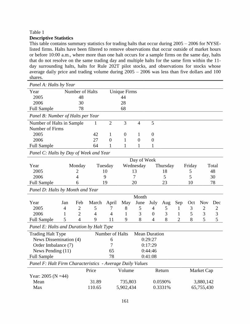
161
Table 1
Descriptive Statistics
This table contains summary statistics for trading halts that occur during 2005 – 2006 for NYSE-
listed firms. Halts have been filtered to remove observations that occur outside of market hours
or before 10:00 a.m., where more than one halt occurs for a sample firms on the same day, halts
that do not resolve on the same trading day and multiple halts for the same firm within the 11-
day surrounding halts, halts for Rule 202T pilot stocks, and observations for stocks whose
average daily price and trading volume during 2005 – 2006 was less than five dollars and 100
shares.
Panel A: Halts by Year
Year Number of Halts Unique Firms
2005 48 44
2006 30 28
Full Sample 78 68
Panel B: Number of Halts per Year
Number of Halts in Sample 1 2 3 4 5
Number of Firms
2005 42 1 0 1 0
2006 27 0 1 0 0
Full Sample 64 1 1 1 1
Panel C: Halts by Day of Week and Year
Day of Week
Year Monday Tuesday Wednesday Thursday Friday Total
2005 2 10 13 18 5 48
2006 4 9 7 5 5 30
Full Sample 6 19 20 23 10 78
Panel D: Halts by Month and Year
Month
Year Jan Feb March April May June July Aug Sep Oct Nov Dec
2005 4 2 5 7 8 5 4 5 1 3 2 2
2006 1 2 4 4 1 3 0 3 1 5 3 3
Full Sample 5 4 9 11 9 8 4 8 2 8 5 5
Panel E: Halts and Duration by Halt Type
Trading Halt Type Number of Halts Mean Duration
News Dissemination (4) 6 0:29:27
Order Imbalance (7) 7 0:17:29
News Pending (11) 65 0:44:46
Full Sample 78 0:41:08
Panel F: Halt Firm Characteristics - Average Daily Values
Price Volume Return Market Cap
Year: 2005 (N =44)
Mean 31.89 735,803 0.0590% 3,880,142
Max 110.65 5,902,434 0.3331% 65,755,430
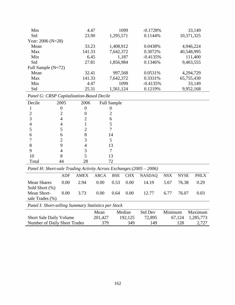
162
Min 4.47 1099 -0.1728% 33,149
Std 23.90 1,295,571 0.1144% 10,371,325
Year: 2006 (N=28)
Mean 33.23 1,408,912 0.0438% 4,946,224
Max 141.33 7,642,372 0.3072% 40,548,995
Min 6.45 1,187 -0.4135% 111,400
Std 27.81 1,856,984 0.1346% 9,403,555
Full Sample (N=72)
Mean 32.41 997,568 0.0531% 4,294,729
Max 141.33 7,642,372 0.3331% 65,755,430
Min 4.47 1099 -0.4135% 33,149
Std 25.31 1,561,124 0.1219% 9,952,168
Panel G: CRSP Capitalization-Based Decile
Decile 2005 2006 Full Sample
1 0 0 0
2 2 0 2
3 4 2 6
4 4 1 5
5 5 2 7
6 6 8 14
7 2 3 5
8 9 4 13
9 4 3 7
10 8 5 13
Total 44 28 72
Panel H: Short-sale Trading Activity Across Exchanges (2005 – 2006)
ADF AMEX ARCA BSE CHX NASDAQ NSX NYSE PHLX
Mean Shares
Sold Short (%)
0.00 2.94 0.00 0.53 0.00 14.19 5.67 76.38 0.29
Mean Short-
sale Trades (%)
0.00 3.73 0.00 0.64 0.00 12.77 6.77 76.07 0.03
Panel I: Short-selling Summary Statistics per Stock
Mean Median Std Dev Minimum Maximum
Short Sale Daily Volume 201,427 192,125 72,895 67,124 1,285,773
Number of Daily Short Trades 379 349 149 128 2,727
163
RESULTS
The model of predation developed by Brunnermeier and Pedersen (2005) describes how
contemporaneous selling by the distressed and predatory traders leads to price overshooting: a
substantial initial price decline is followed by a rebound as predatory traders repurchase shares.
Appendix D contains diagrams that depict the price reaction associated with predation and the
subsequent change in the value of holdings of the predators and the distressed trader. To
determine whether halted stocks in our sample show evidence of predation, we examine halt-day
price movements and attempt to link subsequent returns with the predatory trading behavior of
market participants.
Initial Price Decline
Our hypothesis regarding the price behavior of halted stocks purports that:
H1: Securities undergoing trading halts will demonstrate predatory trading by experiencing
an initial significant price decline.
To identify and measure price declines, we compute, for the halted stocks for 5-minute
intervals on the halt-day , a standardized abnormal return measure:
(1)
164
Where represents the return for stock i during interval j on the halt day,
is the average return for stock i during the pre-halt period (days -30 to -1), and
is the stock’s pre-halt return standard deviation. For example, an abret
value of two indicates that the excess return earned is two return standard deviations greater than
the return in the corresponding interval during the estimation period. Twelve periods are
measured backwards from the beginning of the halt and forward from the resumption of trading.
The abnormal standardized return values are displayed in Figure 1. Preceding the halt,
abret values appear relatively stable and cluster near zero until two periods immediately prior to
the interruption in trading, when a measurable increase is noted from 0.04 to 0.45. An extreme
price movement occurs in period -1, with the abnormal standardized return increasing to 1.30;
this upward trend continues upon the resumption of trading. Prices experience a steep decline as
abret values drop from a peak of 1.46 in period +1 to a low of -2.94 in the following period,
before immediately rebounding to -0.76. The price behavior demonstrated upon the resumption
of trading closely resembles the pattern predicted in the predatory model: an initial price decline,
price overshooting and a subsequent recovery.
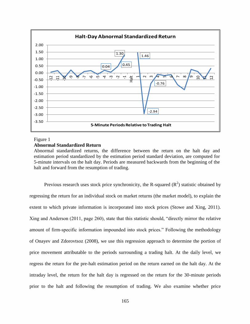
165
Figure 1
Abnormal Standardized Return
Abnormal standardized returns, the difference between the return on the halt day and
estimation period standardized by the estimation period standard deviation, are computed for
5-minute intervals on the halt day. Periods are measured backwards from the beginning of the
halt and forward from the resumption of trading.
Previous research uses stock price synchronicity, the R-squared (R2) statistic obtained by
regressing the return for an individual stock on market returns (the market model), to explain the
extent to which private information is incorporated into stock prices (Stowe and Xing, 2011).
Xing and Anderson (2011, page 260), state that this statistic should, “directly mirror the relative
amount of firm-specific information impounded into stock prices.” Following the methodology
of Onayev and Zdorovtsoz (2008), we use this regression approach to determine the portion of
price movement attributable to the periods surrounding a trading halt. At the daily level, we
regress the return for the pre-halt estimation period on the return earned on the halt day. At the
intraday level, the return for the halt day is regressed on the return for the 30-minute periods
prior to the halt and following the resumption of trading. We also examine whether price
0.040.45
1.301.46
-2.94
-0.76
-3.50
-3.00
-2.50
-2.00
-1.50
-1.00
-0.50
0.00
0.50
1.00
1.50
2.00
-12
-11
-10 -9 -8 -7 -6 -5 -4 -3 -2 -1
Hal
t 1 2 3 4 5 6 7 8 9 10 11 12
5-Minute Periods Relative to Trading Halt
Halt-Day Abnormal Standardized Return
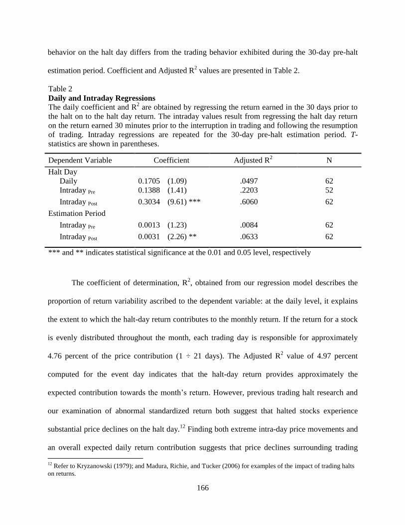
166
behavior on the halt day differs from the trading behavior exhibited during the 30-day pre-halt
estimation period. Coefficient and Adjusted R2 values are presented in Table 2.
Table 2
Daily and Intraday Regressions
The daily coefficient and R2 are obtained by regressing the return earned in the 30 days prior to
the halt on to the halt day return. The intraday values result from regressing the halt day return
on the return earned 30 minutes prior to the interruption in trading and following the resumption
of trading. Intraday regressions are repeated for the 30-day pre-halt estimation period. T-
statistics are shown in parentheses.
Dependent Variable Coefficient Adjusted R2 N
Halt Day
Daily 0.1705 (1.09) .0497 62
Intraday Pre 0.1388 (1.41) .2203 52
Intraday Post 0.3034 (9.61) *** .6060 62
Estimation Period
Intraday Pre 0.0013 (1.23) .0084 62
Intraday Post 0.0031 (2.26) ** .0633 62
*** and ** indicates statistical significance at the 0.01 and 0.05 level, respectively
The coefficient of determination, R2, obtained from our regression model describes the
proportion of return variability ascribed to the dependent variable: at the daily level, it explains
the extent to which the halt-day return contributes to the monthly return. If the return for a stock
is evenly distributed throughout the month, each trading day is responsible for approximately
4.76 percent of the price contribution (1 ÷ 21 days). The Adjusted R2 value of 4.97 percent
computed for the event day indicates that the halt-day return provides approximately the
expected contribution towards the month’s return. However, previous trading halt research and
our examination of abnormal standardized return both suggest that halted stocks experience
substantial price declines on the halt day.12
Finding both extreme intra-day price movements and
an overall expected daily return contribution suggests that price declines surrounding trading
12
Refer to Kryzanowski (1979); and Madura, Richie, and Tucker (2006) for examples of the impact of trading halts
on returns.

167
halts are accompanied by a rebound - stock prices recover to near their original levels by the end
of the trading day. This result lends credence to the presence of the price decline and reversal
associated with predation.
At the intraday level, the R2 values describe how the 30-minute period pre- and post-halt
returns contribute to the return earned on the halt day. Each 30-minute trading period, on
average, should provide approximately 7.69 percent of price contribution (1 ÷ 13 periods). For
the estimation period, the contribution in the 30 minutes prior to the trading halt is much smaller
at only 0.84 percent, but the post-halt period Adjusted R2 of 6.33 percent is at a more-anticipated
level. In contrast, halt-day values are substantially elevated - over 22 and 60 percent of price
contribution occurs in the pre- and post-halt periods, respectively. This finding corresponds with
the considerable price movement immediately prior to the halt and following the resumption of
trading noted in our examination of abnormal standardized return.
To determine if there exists a causal relation between the trading activity and price
movement surrounding halts, we compute Granger Causality for 5-minute periods on the halt day
between short volume, non-short volume, and returns. Periods are measured backward from the
implementation of the halt and forward from the resumption of trading. Partial canonical and
cross correlations, which demonstrate significance for up to nine intervals, are used to determine
the appropriate number of lags to examine. These results are presented in Panel A of Table 3.
Chi-Square and associated p-values describing the causal relation between non-short
volume, short volume, and returns are listed in Table 3, Panel B. The null hypothesis of the
Granger Causality Wald test purports that the value of the dependent variable is influenced only
by itself; an alpha value indicating statistical significance allows us to reject the null hypothesis
and establishes that one variable exerts influence over another.
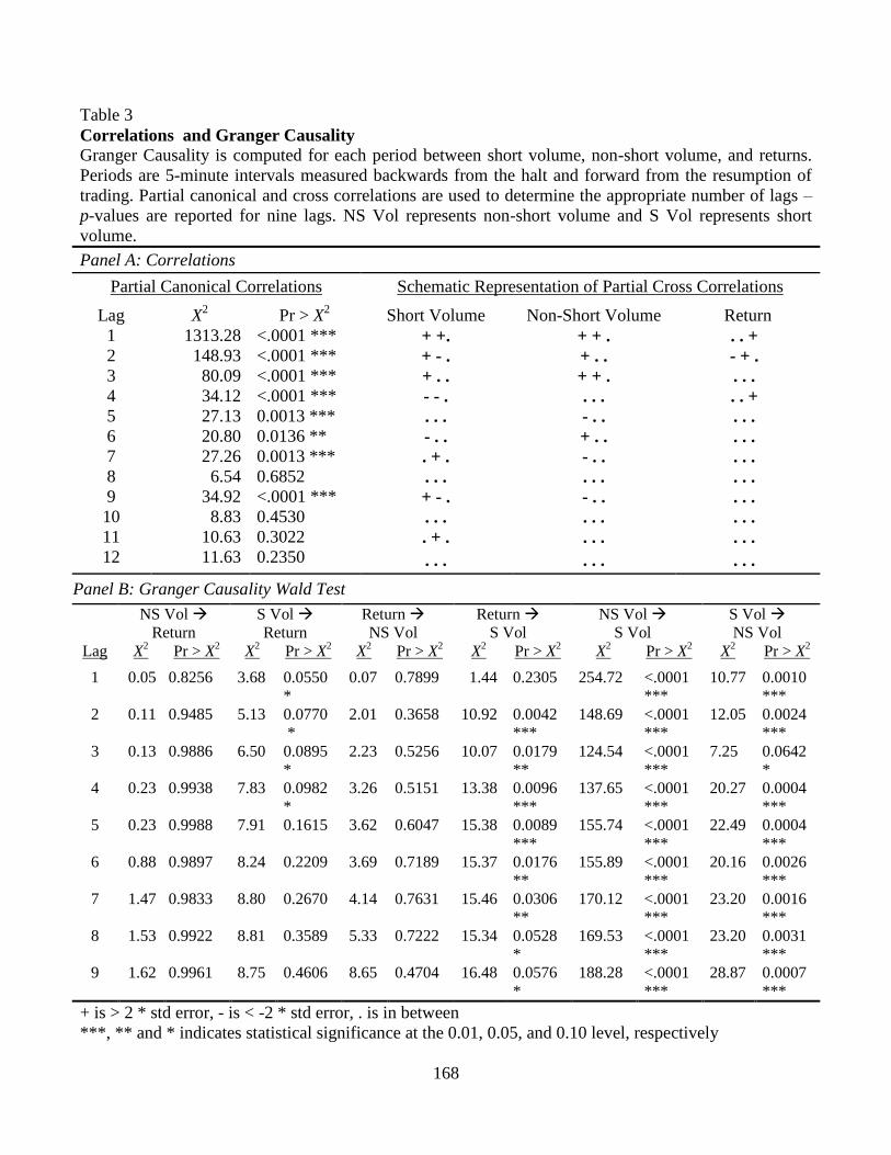
168
Table 3
Correlations and Granger Causality
Granger Causality is computed for each period between short volume, non-short volume, and returns.
Periods are 5-minute intervals measured backwards from the halt and forward from the resumption of
trading. Partial canonical and cross correlations are used to determine the appropriate number of lags –
p-values are reported for nine lags. NS Vol represents non-short volume and S Vol represents short
volume.
Panel A: Correlations
Partial Canonical Correlations Schematic Representation of Partial Cross Correlations
Lag X2 Pr > X
2 Short Volume Non-Short Volume Return
1 1313.28 <.0001 *** + +. + + . . . +
2 148.93 <.0001 *** + - . + . . - + .
3 80.09 <.0001 *** + . . + + . . . .
4 34.12 <.0001 *** - - . . . . . . +
5 27.13 0.0013 *** . . . - . . . . .
6 20.80 0.0136 ** - . . + . . . . .
7 27.26 0.0013 *** . + . - . . . . .
8 6.54 0.6852 . . . . . . . . .
9 34.92 <.0001 *** + - . - . . . . .
10 8.83 0.4530 . . . . . . . . .
11 10.63 0.3022 . + . . . . . . .
12 11.63 0.2350 . . . . . . . . .
Panel B: Granger Causality Wald Test
NS Vol
Return
S Vol
Return
Return
NS Vol
Return
S Vol
NS Vol
S Vol
S Vol
NS Vol
Lag X2 Pr > X
2 X
2 Pr > X
2 X
2 Pr > X
2 X
2 Pr > X
2 X
2 Pr > X
2 X
2 Pr > X
2
1 0.05 0.8256 3.68 0.0550
*
0.07 0.7899 1.44 0.2305 254.72 <.0001
***
10.77 0.0010
***
2 0.11 0.9485 5.13 0.0770
*
2.01 0.3658 10.92 0.0042
***
148.69 <.0001
***
12.05 0.0024
***
3 0.13 0.9886 6.50 0.0895
*
2.23 0.5256 10.07 0.0179
**
124.54 <.0001
***
7.25 0.0642
*
4 0.23 0.9938 7.83 0.0982
*
3.26 0.5151 13.38 0.0096
***
137.65 <.0001
***
20.27 0.0004
***
5 0.23 0.9988 7.91 0.1615 3.62 0.6047 15.38 0.0089
***
155.74 <.0001
***
22.49 0.0004
***
6 0.88 0.9897 8.24 0.2209 3.69 0.7189 15.37 0.0176
**
155.89 <.0001
***
20.16 0.0026
***
7 1.47 0.9833 8.80 0.2670 4.14 0.7631 15.46 0.0306
**
170.12 <.0001
***
23.20 0.0016
***
8 1.53 0.9922 8.81 0.3589 5.33 0.7222 15.34 0.0528
*
169.53 <.0001
***
23.20 0.0031
***
9 1.62 0.9961 8.75 0.4606 8.65 0.4704 16.48 0.0576
*
188.28 <.0001
***
28.87 0.0007
***
+ is > 2 * std error, - is < -2 * std error, . is in between
***, ** and * indicates statistical significance at the 0.01, 0.05, and 0.10 level, respectively
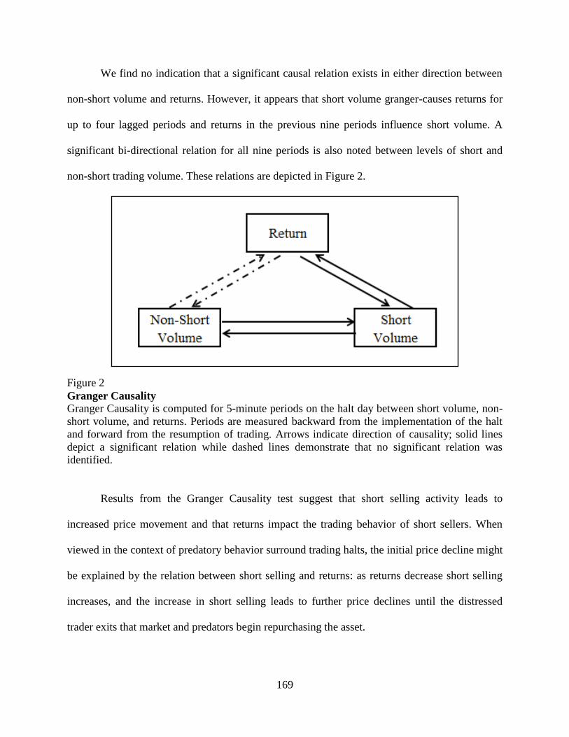
169
We find no indication that a significant causal relation exists in either direction between
non-short volume and returns. However, it appears that short volume granger-causes returns for
up to four lagged periods and returns in the previous nine periods influence short volume. A
significant bi-directional relation for all nine periods is also noted between levels of short and
non-short trading volume. These relations are depicted in Figure 2.
Figure 2
Granger Causality
Granger Causality is computed for 5-minute periods on the halt day between short volume, non-
short volume, and returns. Periods are measured backward from the implementation of the halt
and forward from the resumption of trading. Arrows indicate direction of causality; solid lines
depict a significant relation while dashed lines demonstrate that no significant relation was
identified.
Results from the Granger Causality test suggest that short selling activity leads to
increased price movement and that returns impact the trading behavior of short sellers. When
viewed in the context of predatory behavior surround trading halts, the initial price decline might
be explained by the relation between short selling and returns: as returns decrease short selling
increases, and the increase in short selling leads to further price declines until the distressed
trader exits that market and predators begin repurchasing the asset.

170
In support of Hypothesis 1, the securities of sample firms evidence behavior that might
be attributed to predatory trading activity, particularly on the part of short sellers. Prices
demonstrate, following the resumption of trading, the sharp decline and rebound described in
predatory models. Intraday price contribution values indicate increased price movement
surrounding the halt, while the proportional daily price contribution of the halt day in monthly
returns lends support to the presence of a price rebound.
Order Imbalances
The trading model of predation presented in previous literature suggests that predatory
traders initially engage in contemporaneous selling while the distressed trader is attempting to
liquidate his position, then predators switch roles and begin repurchasing the asset. This trading
behavior should lead to order imbalances, with higher levels of selling as prices decline and
increased buying as prices rebound. Brown, Walsh, and Yuen (1997 page 539) state, “… a
temporal imbalance between buy and sell orders arriving at a market increases the likelihood that
informed traders are attempting to pre-empt good or bad news ….” Chordia, Roll, and
Subrahmanyam (2002 page 118) find that excess buy (sell) orders drive up (down) security
prices; they state, “For an individual stock, a large order imbalance could be random or induced
by either public or private information.”
Our hypothesis regarding the relation between buy and sell orders for halted stocks
suggest that:
H2: Securities undergoing trading halts will demonstrate predatory trading by experiencing
event-day order imbalances caused by both non-short and short selling.
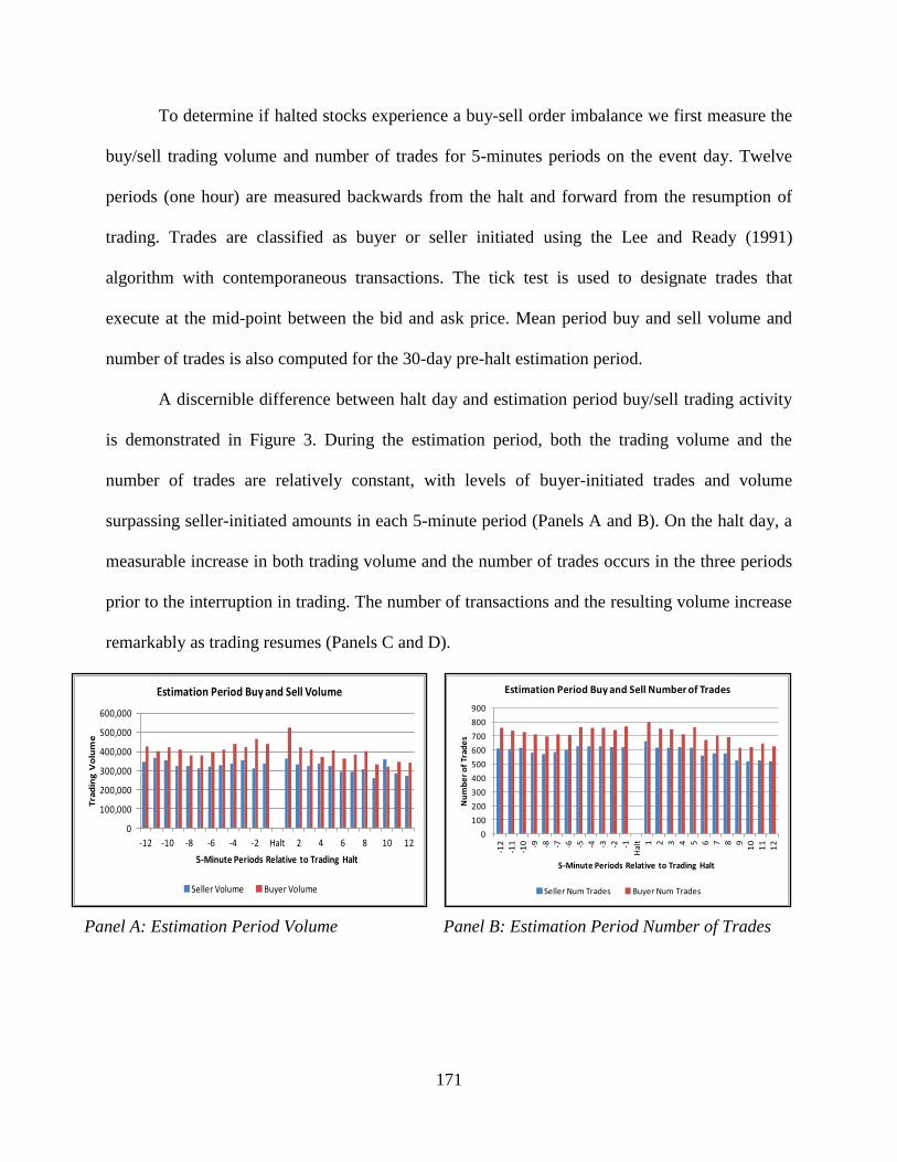
171
To determine if halted stocks experience a buy-sell order imbalance we first measure the
buy/sell trading volume and number of trades for 5-minutes periods on the event day. Twelve
periods (one hour) are measured backwards from the halt and forward from the resumption of
trading. Trades are classified as buyer or seller initiated using the Lee and Ready (1991)
algorithm with contemporaneous transactions. The tick test is used to designate trades that
execute at the mid-point between the bid and ask price. Mean period buy and sell volume and
number of trades is also computed for the 30-day pre-halt estimation period.
A discernible difference between halt day and estimation period buy/sell trading activity
is demonstrated in Figure 3. During the estimation period, both the trading volume and the
number of trades are relatively constant, with levels of buyer-initiated trades and volume
surpassing seller-initiated amounts in each 5-minute period (Panels A and B). On the halt day, a
measurable increase in both trading volume and the number of trades occurs in the three periods
prior to the interruption in trading. The number of transactions and the resulting volume increase
remarkably as trading resumes (Panels C and D).
Panel A: Estimation Period Volume Panel B: Estimation Period Number of Trades
0
100,000
200,000
300,000
400,000
500,000
600,000
-12 -10 -8 -6 -4 -2 Halt 2 4 6 8 10 12
Tra
din
g V
olu
me
5-Minute Periods Relative to Trading Halt
Estimation Period Buy and Sell Volume
Seller Volume Buyer Volume
0
100
200
300
400
500
600
700
800
900
-12
-11
-10 -9 -8 -7 -6 -5 -4 -3 -2 -1
Hal
t 1 2 3 4 5 6 7 8 9
10
11
12
Nu
mb
er
of
Trad
es
5-Minute Periods Relative to Trading Halt
Estimation Period Buy and Sell Number of Trades
Seller Num Trades Buyer Num Trades
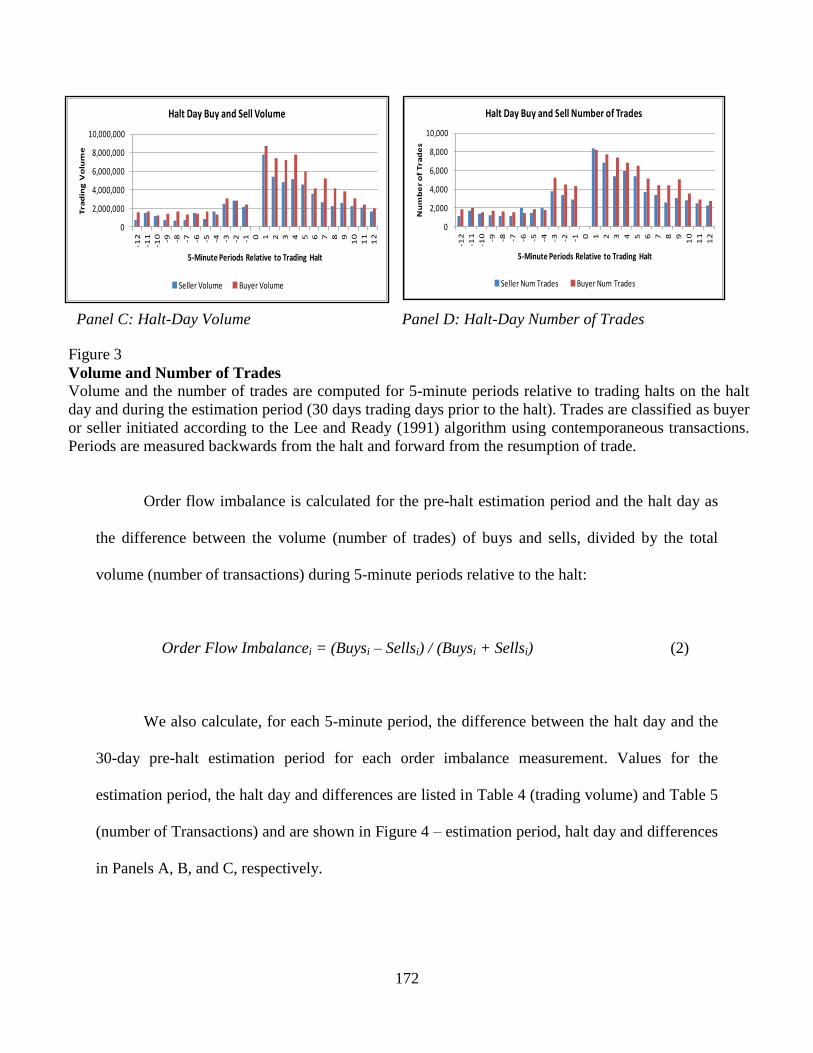
172
Panel C: Halt-Day Volume Panel D: Halt-Day Number of Trades
Figure 3
Volume and Number of Trades
Volume and the number of trades are computed for 5-minute periods relative to trading halts on the halt
day and during the estimation period (30 days trading days prior to the halt). Trades are classified as buyer
or seller initiated according to the Lee and Ready (1991) algorithm using contemporaneous transactions.
Periods are measured backwards from the halt and forward from the resumption of trade.
Order flow imbalance is calculated for the pre-halt estimation period and the halt day as
the difference between the volume (number of trades) of buys and sells, divided by the total
volume (number of transactions) during 5-minute periods relative to the halt:
Order Flow Imbalancei = (Buysi – Sellsi) / (Buysi + Sellsi) (2)
We also calculate, for each 5-minute period, the difference between the halt day and the
30-day pre-halt estimation period for each order imbalance measurement. Values for the
estimation period, the halt day and differences are listed in Table 4 (trading volume) and Table 5
(number of Transactions) and are shown in Figure 4 – estimation period, halt day and differences
in Panels A, B, and C, respectively.
0
2,000,000
4,000,000
6,000,000
8,000,000
10,000,000-1
2
-11
-10 -9 -8 -7 -6 -5 -4 -3 -2 -1 0 1 2 3 4 5 6 7 8 9
10
11
12
Tra
din
g V
olu
me
5-Minute Periods Relative to Trading Halt
Halt Day Buy and Sell Volume
Seller Volume Buyer Volume
0
2,000
4,000
6,000
8,000
10,000
-12
-11
-10 -9 -8 -7 -6 -5 -4 -3 -2 -1 0 1 2 3 4 5 6 7 8 9
10
11
12
Nu
mb
er
of
Tra
de
s
5-Minute Periods Relative to Trading Halt
Halt Day Buy and Sell Number of Trades
Seller Num Trades Buyer Num Trades

173
Table 4
Order Imbalance – Trading Volume Order flow imbalance is computed for the 30-day pre-halt estimation period and the event day as
the difference between the volume of buys and sells, divided by the total volume over the period.
The differences in order imbalance ratios are computed between the halt and the estimation
period. Trades are classified as buyer or seller initiated using the Lee and Ready algorithm and
contemporaneous transactions. t-statistics are listed in parentheses
Period Estimation Period Halt Day Differences
-12 0.0632 (6.16) *** 0.0305 (0.48) -0.0457 (-0.74)
-11 0.0592 (4.77) *** 0.1234 (1.81) * 0.0572 (0.79)
-10 0.0842 (6.64) *** 0.0927 (1.33) 0.0039 (0.05)
-9 0.0856 (7.18) *** 0.1308 (1.92) * 0.0473 (0.69)
-8 0.0718 (4.62) *** 0.1055 (1.52) 0.0283 (0.39)
-7 0.0870 (7.06) *** 0.1321 (2.22) ** 0.0372 (0.66)
-6 0.0904 (6.61) *** 0.0539 (0.69) -0.0273 (-0.33)
-5 0.0780 (5.52) *** 0.1426 (2.07) ** 0.0623 (0.92)
-4 0.0653 (5.68) *** 0.0629 (0.92) 0.0027 (0.04)
-3 0.0848 (5.82) *** 0.0595 (0.86) -0.0402 (-0.60)
-2 0.0844 (6.57) *** 0.0436 (0.66) -0.0393 (-0.61)
-1 0.0989 (7.08) *** 0.0919 (1.42) -0.0076 (-0.11)
Halt
1 0.0928 (7.05) *** 0.1032 (1.87) * 0.0632 (1.04)
2 0.0831 (6.70) *** 0.1980 (4.27) *** 0.1112 (2.21) **
3 0.0764 (7.52) *** 0.2545 (4.83) *** 0.1574 (2.97) ***
4 0.0587 (4.01) *** 0.1593 (2.88) *** 0.1118 (2.08) **
5 0.0861 (7.06) *** 0.1222 (2.14) ** 0.0497 (0.75)
6 0.0884 (7.09) *** 0.1004 (1.80) * 0.0172 (0.29)
7 0.0813 (7.08) *** 0.0720 (1.18) 0.0081 (0.13)
8 0.0836 (7.32) *** 0.1370 (1.96) * 0.0630 (0.88)
9 0.0566 (4.40) *** 0.0906 (1.37) 0.0403 (0.60)
10 0.0779 (8.19) *** 0.1156 (1.72) * 0.0396 (0.56)
11 0.0792 (5.58) *** 0.1707 (2.80) *** 0.1055 (1.57)
12 0.0889 (5.81) *** 0.1228 (1.71) * 0.0370 (0.49)
***, ** and * indicates statistical significance at the 0.01, 0.05 and 0.10 level respectively
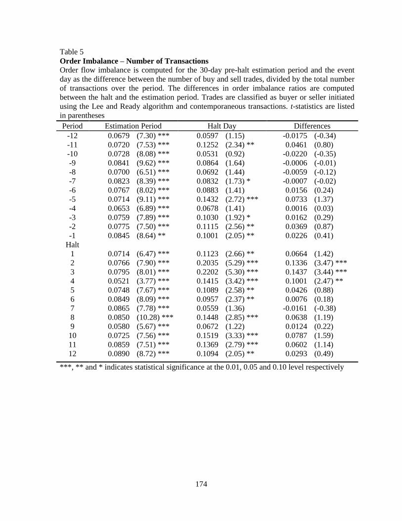
174
Table 5
Order Imbalance – Number of Transactions Order flow imbalance is computed for the 30-day pre-halt estimation period and the event
day as the difference between the number of buy and sell trades, divided by the total number
of transactions over the period. The differences in order imbalance ratios are computed
between the halt and the estimation period. Trades are classified as buyer or seller initiated
using the Lee and Ready algorithm and contemporaneous transactions. t-statistics are listed
in parentheses
Period Estimation Period Halt Day Differences
-12 0.0679 (7.30) *** 0.0597 (1.15) -0.0175 (-0.34)
-11 0.0720 (7.53) *** 0.1252 (2.34) ** 0.0461 (0.80)
-10 0.0728 (8.08) *** 0.0531 (0.92) -0.0220 (-0.35)
-9 0.0841 (9.62) *** 0.0864 (1.64) -0.0006 (-0.01)
-8 0.0700 (6.51) *** 0.0692 (1.44) -0.0059 (-0.12)
-7 0.0823 (8.39) *** 0.0832 (1.73) * -0.0007 (-0.02)
-6 0.0767 (8.02) *** 0.0883 (1.41) 0.0156 (0.24)
-5 0.0714 (9.11) *** 0.1432 (2.72) *** 0.0733 (1.37)
-4 0.0653 (6.89) *** 0.0678 (1.41) 0.0016 (0.03)
-3 0.0759 (7.89) *** 0.1030 (1.92) * 0.0162 (0.29)
-2 0.0775 (7.50) *** 0.1115 (2.56) ** 0.0369 (0.87)
-1 0.0845 (8.64) ** 0.1001 (2.05) ** 0.0226 (0.41)
Halt
1 0.0714 (6.47) *** 0.1123 (2.66) ** 0.0664 (1.42)
2 0.0766 (7.90) *** 0.2035 (5.29) *** 0.1336 (3.47) ***
3 0.0795 (8.01) *** 0.2202 (5.30) *** 0.1437 (3.44) ***
4 0.0521 (3.77) *** 0.1415 (3.42) *** 0.1001 (2.47) **
5 0.0748 (7.67) *** 0.1089 (2.58) ** 0.0426 (0.88)
6 0.0849 (8.09) *** 0.0957 (2.37) ** 0.0076 (0.18)
7 0.0865 (7.78) *** 0.0559 (1.36) -0.0161 (-0.38)
8 0.0850 (10.28) *** 0.1448 (2.85) *** 0.0638 (1.19)
9 0.0580 (5.67) *** 0.0672 (1.22) 0.0124 (0.22)
10 0.0725 (7.56) *** 0.1519 (3.33) *** 0.0787 (1.59)
11 0.0859 (7.51) *** 0.1369 (2.79) *** 0.0602 (1.14)
12 0.0890 (8.72) *** 0.1094 (2.05) ** 0.0293 (0.49)
***, ** and * indicates statistical significance at the 0.01, 0.05 and 0.10 level respectively
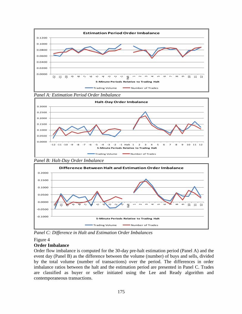
175
Panel A: Estimation Period Order Imbalance
Panel B: Halt-Day Order Imbalance
Panel C: Difference in Halt and Estimation Order Imbalances
Figure 4
Order Imbalance
Order flow imbalance is computed for the 30-day pre-halt estimation period (Panel A) and the
event day (Panel B) as the difference between the volume (number) of buys and sells, divided
by the total volume (number of transactions) over the period. The differences in order
imbalance ratios between the halt and the estimation period are presented in Panel C. Trades
are classified as buyer or seller initiated using the Lee and Ready algorithm and
contemporaneous transactions.
0.0000
0.0200
0.0400
0.0600
0.0800
0.1000
0.1200
-12
-11
-10 -9 -8 -7 -6 -5 -4 -3 -2 -1
Halt 1 2 3 4 5 6 7 8 9 10 11 12
5-Minute Periods Relative to Trading Halt
Estimation Period Order Imbalance
Trading Volume Number of Trades
0.0000
0.0500
0.1000
0.1500
0.2000
0.2500
0.3000
-12 -11 -10 -9 -8 -7 -6 -5 -4 -3 -2 -1 Halt 1 2 3 4 5 6 7 8 9 10 11 12
5-Minute Periods Relative to Trading Halt
Halt-Day Order Imbalance
Trading Volume Number of Trades
-0.1000
-0.0500
0.0000
0.0500
0.1000
0.1500
0.2000
-12
-11
-10 -9 -8 -7 -6 -5 -4 -3 -2 -1
Halt 1 2 3 4 5 6 7 8 9 10 11 12
5-Minute Periods Relative to Trading Halt
Difference Between Halt and Estimation Order Imbalance
Trading Volume Number of Trades

176
During the estimation period, order imbalance metrics for both trading volume and
number of trades are positive and relatively stable for all periods, ranging from 5.21 to 9.89
percent. Previous studies support the presence of a higher number of buyer-initiated transactions:
Chordia and Subrahmanyam (2002); and Chordia et al. (2002) find, in their examination of daily
trading on the NYSE, positive order imbalances (buys exceeding sells) for the number of trades,
shares, and dollar volume.
On the halt day, order imbalance metrics for volume and number of trades range from
3.05 to 14.26 percent in the periods preceding the halt. Upon the resumption of trading, both
measurements increase significantly, with maximum values, occurring in period +3, of 25.45
percent for trading volume and 22.02 percent for the number of trades; these metrics remain
elevated for six consecutive post-halt periods. The difference variable demonstrates a
corresponding significant increase in periods +2 through +4, when the order imbalance is
approximately 11 to 16 percent higher than on non-halt days.
Chordia et al. (2002) examine daily order imbalances on the NYSE. They find that order
imbalance increases following a market decline and selling activity is heightened following
market rises. We are able to identify this pattern in our results: order imbalance metrics peak in
period +3 after the negative abnormal standardized return in period +2, and more seller-initiated
activity (lower order imbalance values) occur in periods +4 though +6 as stock prices rebound
and abret values increase.
In all halt-day periods, buyer-initiated activity exceeds the activity initiated by sellers.
The largest buy/sell discrepancy occurs upon the post-halt continuation of trading. This result is
in direct opposition to our expectations: an increase in seller-initiated activity is anticipated

177
directly after the halt during the interval when prices decline and positive order imbalances are
expected to correspond with buyer-initiated activity during the price rebound.
This unexpected result might be attributed to the manner in which the Lee-Ready
algorithm categorizes short sales. Asquith, Oman, and Safaya (2010), describe how previous
studies analyzing the Lee-Ready algorithm report 72 to 93 percent accuracy rates. However,
these tests are performed prior to the 2001 conversion to reporting market prices in decimals –
narrower spreads resulting from decimalization potentially make it more difficult to classify
trades accurately. Additionally, these researchers explain how the uptick rule, which allows
execution of a short sale only on an uptick or zero tick, may cause short sales to execute at a
price above the bid-ask spread midpoint and subsequently result in the improper classification of
short sale transactions as buyer-initiated. Results from this research suggest that the Lee-Ready
algorithm overwhelmingly classifies short transactions, which represent nearly 30 percent of
trading volume, as buyer-initiated. Specifically, they find that the Lee-Ready algorithm, using
contemporaneous transactions, classifies 66.5 percent of short trades as buyer-initiated. When
differentiating between stocks participating in the SEC Pilot study (Rule 202T), they find, during
June and December of 2005, between 85.1 and 88.0 percent of short sales for a sample of NYSE
non-pilot stocks are classified as buyer-initiated.
To determine if this explanation is applicable to our research, we compute, for both the
halt day and the 30-day pre-halt estimation period, levels of non-short and short volume, and the
percent short volume represents of total volume during each of the twelve pre- and post-halt
periods (shown in Figure 5). The estimation period results demonstrate relatively constant
values, with short selling activity representing approximately twenty percent of overall trading
volume (Panels A and B). On the halt day, however, we identify several key differences. During
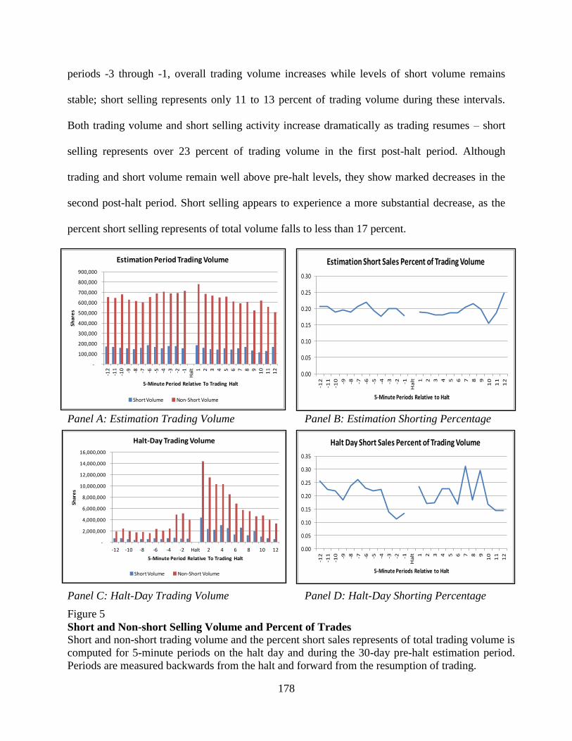
178
periods -3 through -1, overall trading volume increases while levels of short volume remains
stable; short selling represents only 11 to 13 percent of trading volume during these intervals.
Both trading volume and short selling activity increase dramatically as trading resumes – short
selling represents over 23 percent of trading volume in the first post-halt period. Although
trading and short volume remain well above pre-halt levels, they show marked decreases in the
second post-halt period. Short selling appears to experience a more substantial decrease, as the
percent short selling represents of total volume falls to less than 17 percent.
Panel A: Estimation Trading Volume Panel B: Estimation Shorting Percentage
Panel C: Halt-Day Trading Volume Panel D: Halt-Day Shorting Percentage
Figure 5
Short and Non-short Selling Volume and Percent of Trades
Short and non-short trading volume and the percent short sales represents of total trading volume is
computed for 5-minute periods on the halt day and during the 30-day pre-halt estimation period.
Periods are measured backwards from the halt and forward from the resumption of trading.
-
100,000
200,000
300,000
400,000
500,000
600,000
700,000
800,000
900,000
-12
-11
-10 -9 -8 -7 -6 -5 -4 -3 -2 -1
Hal
t 1 2 3 4 5 6 7 8 9
10
11
12
Shar
es
5-Minute Period Relative To Trading Halt
Estimation Period Trading Volume
Short Volume Non-Short Volume
0.00
0.05
0.10
0.15
0.20
0.25
0.30
-12
-11
-10 -9 -8 -7 -6 -5 -4 -3 -2 -1
Ha
lt 1 2 3 4 5 6 7 8 9
10
11
12
5-Minute Periods Relative to Halt
Estimation Short Sales Percent of Trading Volume
-
2,000,000
4,000,000
6,000,000
8,000,000
10,000,000
12,000,000
14,000,000
16,000,000
-12 -10 -8 -6 -4 -2 Halt 2 4 6 8 10 12
Shar
es
5-Minute Period Relative To Trading Halt
Halt-Day Trading Volume
Short Volume Non-Short Volume
0.00
0.05
0.10
0.15
0.20
0.25
0.30
0.35
-12
-11
-10 -9 -8 -7 -6 -5 -4 -3 -2 -1
Ha
lt 1 2 3 4 5 6 7 8 9
10
11
12
5-Minute Periods Relative to Halt
Halt Day Short Sales Percent of Trading Volume

179
We are able to identify the anticipated inverse relation between short selling levels and
returns by relying on Granger causality test results: lagged short selling impacts returns. Using
one period lags, we categorize, for three post-halt periods, short selling levels as high or low,
depending on their position relative to the approximate 20 percent estimation period average
established from Figure 5 Panel B. We also note whether abnormal standardized returns increase
or decrease from the previous period. The results, shown below, indicate that 1) lagged short
selling levels are low in period +1 as abnormal standardized returns peak, 2) lagged short selling
increases in period +2 as abnormal standardized returns fall (increased selling activity and
associated price declines), and 3) lagged short selling is lower in period +3, as abnormal
standardized returns begin to rebound. This model provides a possible scenario in which short
sellers engage in predatory activity surrounding halts in trading.
Period +1 +2 +3
Short Selling Lagged 1 Period Low High Low
Abnormal Return Increase Decrease Increase
To explore further the role of short sellers surrounding halts in trading, we calculate two
short-selling metrics. First, abshvol, a standardized short selling measure, is computed for halted
stocks for 5-minute intervals on the halt day (Shkilko et al. 2012):
(3)
Where represents the volume of shares shorted for stock i during interval j on the
halt day, is the average short volume for the pre-halt period (days -30 to -1), and
is the standard deviation of the short volume during the pre-halt
period. Periods are measured backwards from the halt and forward from the resumption of
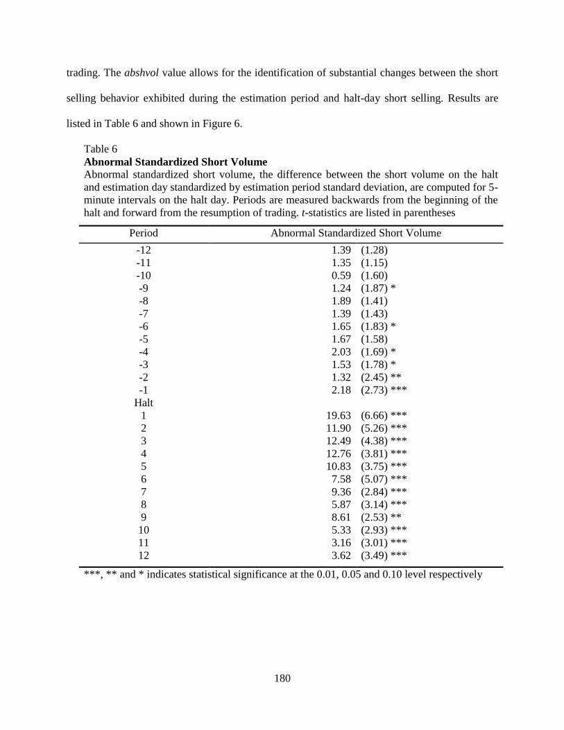
180
trading. The abshvol value allows for the identification of substantial changes between the short
selling behavior exhibited during the estimation period and halt-day short selling. Results are
listed in Table 6 and shown in Figure 6.
Table 6
Abnormal Standardized Short Volume Abnormal standardized short volume, the difference between the short volume on the halt
and estimation day standardized by estimation period standard deviation, are computed for 5-
minute intervals on the halt day. Periods are measured backwards from the beginning of the
halt and forward from the resumption of trading. t-statistics are listed in parentheses
Period Abnormal Standardized Short Volume
-12 1.39 (1.28)
-11 1.35 (1.15)
-10 0.59 (1.60)
-9 1.24 (1.87) *
-8 1.89 (1.41)
-7 1.39 (1.43)
-6 1.65 (1.83) *
-5 1.67 (1.58)
-4 2.03 (1.69) *
-3 1.53 (1.78) *
-2 1.32 (2.45) **
-1 2.18 (2.73) ***
Halt
1 19.63 (6.66) ***
2 11.90 (5.26) ***
3 12.49 (4.38) ***
4 12.76 (3.81) ***
5 10.83 (3.75) ***
6 7.58 (5.07) ***
7 9.36 (2.84) ***
8 5.87 (3.14) ***
9 8.61 (2.53) **
10 5.33 (2.93) ***
11 3.16 (3.01) ***
12 3.62 (3.49) ***
***, ** and * indicates statistical significance at the 0.01, 0.05 and 0.10 level respectively
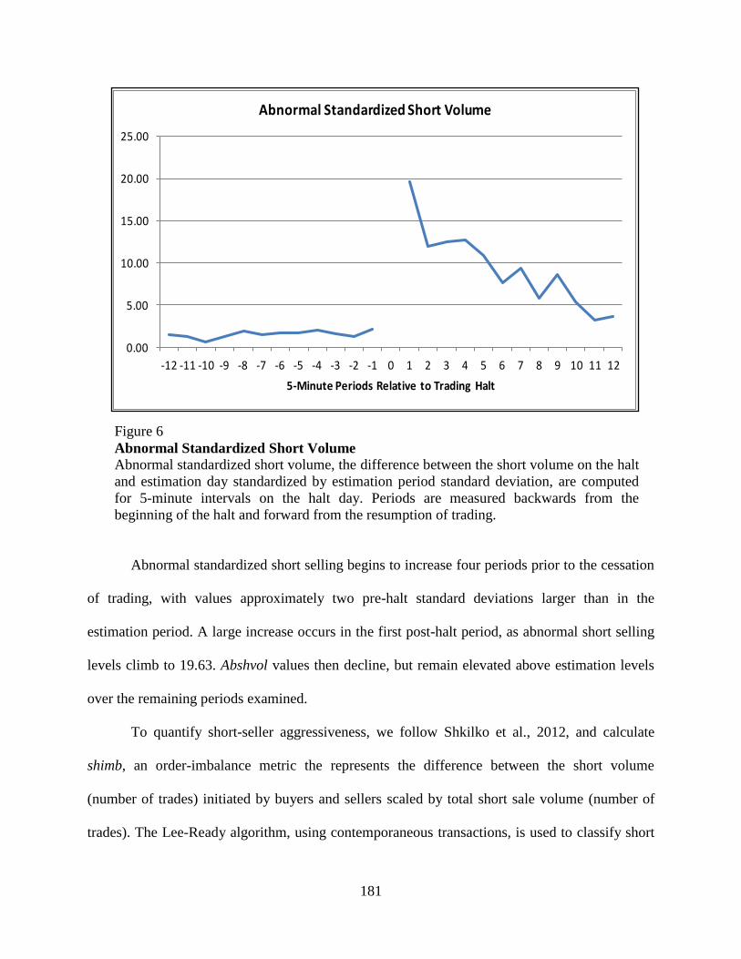
181
Figure 6
Abnormal Standardized Short Volume
Abnormal standardized short volume, the difference between the short volume on the halt
and estimation day standardized by estimation period standard deviation, are computed
for 5-minute intervals on the halt day. Periods are measured backwards from the
beginning of the halt and forward from the resumption of trading.
Abnormal standardized short selling begins to increase four periods prior to the cessation
of trading, with values approximately two pre-halt standard deviations larger than in the
estimation period. A large increase occurs in the first post-halt period, as abnormal short selling
levels climb to 19.63. Abshvol values then decline, but remain elevated above estimation levels
over the remaining periods examined.
To quantify short-seller aggressiveness, we follow Shkilko et al., 2012, and calculate
shimb, an order-imbalance metric the represents the difference between the short volume
(number of trades) initiated by buyers and sellers scaled by total short sale volume (number of
trades). The Lee-Ready algorithm, using contemporaneous transactions, is used to classify short
0.00
5.00
10.00
15.00
20.00
25.00
-12 -11 -10 -9 -8 -7 -6 -5 -4 -3 -2 -1 0 1 2 3 4 5 6 7 8 9 10 11 12
5-Minute Periods Relative to Trading Halt
Abnormal Standardized Short Volume
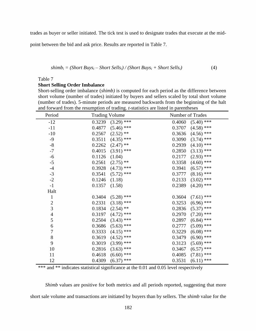
182
trades as buyer or seller initiated. The tick test is used to designate trades that execute at the mid-
point between the bid and ask price. Results are reported in Table 7.
shimbi = (Short Buysi – Short Sellsi) / (Short Buysi + Short Sellsi) (4)
Table 7
Short Selling Order Imbalance Short-selling order imbalance (shimb) is computed for each period as the difference between
short volume (number of trades) initiated by buyers and sellers scaled by total short volume
(number of trades). 5-minute periods are measured backwards from the beginning of the halt
and forward from the resumption of trading. t-statistics are listed in parentheses
Period Trading Volume Number of Trades
-12 0.3239 (3.29) *** 0.4060 (5.40) ***
-11 0.4877 (5.46) *** 0.3707 (4.58) ***
-10 0.2567 (2.52) ** 0.3636 (4.56) ***
-9 0.3511 (4.35) *** 0.3090 (3.74) ***
-8 0.2262 (2.47) ** 0.2939 (4.10) ***
-7 0.4015 (3.91) *** 0.2850 (3.13) ***
-6 0.1126 (1.04) 0.2177 (2.93) ***
-5 0.2561 (2.75) ** 0.3358 (4.60) ***
-4 0.3928 (4.73) *** 0.3941 (6.57) ***
-3 0.3541 (5.72) *** 0.3777 (8.16) ***
-2 0.1246 (1.18) 0.2133 (3.02) ***
-1 0.1357 (1.58) 0.2389 (4.20) ***
Halt
1 0.3404 (5.28) *** 0.3604 (7.61) ***
2 0.2331 (3.18) *** 0.3253 (6.96) ***
3 0.1834 (2.54) ** 0.2836 (5.37) ***
4 0.3197 (4.72) *** 0.2970 (7.20) ***
5 0.2504 (3.43) *** 0.2897 (6.84) ***
6 0.3686 (5.63) *** 0.2777 (5.09) ***
7 0.3333 (4.15) *** 0.3229 (6.08) ***
8 0.3619 (4.52) *** 0.3479 (6.90) ***
9 0.3019 (3.99) *** 0.3123 (5.69) ***
10 0.2816 (3.63) *** 0.3467 (6.57) ***
11 0.4618 (6.60) *** 0.4085 (7.81) ***
12 0.4309 (6.37) *** 0.3531 (6.11) ***
*** and ** indicates statistical significance at the 0.01 and 0.05 level respectively
Shimb values are positive for both metrics and all periods reported, suggesting that more
short sale volume and transactions are initiated by buyers than by sellers. The shimb value for the
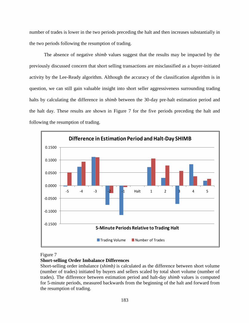
183
number of trades is lower in the two periods preceding the halt and then increases substantially in
the two periods following the resumption of trading.
The absence of negative shimb values suggest that the results may be impacted by the
previously discussed concern that short selling transactions are misclassified as a buyer-initiated
activity by the Lee-Ready algorithm. Although the accuracy of the classification algorithm is in
question, we can still gain valuable insight into short seller aggressiveness surrounding trading
halts by calculating the difference in shimb between the 30-day pre-halt estimation period and
the halt day. These results are shown in Figure 7 for the five periods preceding the halt and
following the resumption of trading.
Figure 7
Short-selling Order Imbalance Differences
Short-selling order imbalance (shimb) is calculated as the difference between short volume
(number of trades) initiated by buyers and sellers scaled by total short volume (number of
trades). The difference between estimation period and halt-day shimb values is computed
for 5-minute periods, measured backwards from the beginning of the halt and forward from
the resumption of trading.
-0.1500
-0.1000
-0.0500
0.0000
0.0500
0.1000
0.1500
-5 -4 -3 -2 -1 Halt 1 2 3 4 5
5-Minute Periods Relative to Trading Halt
Difference in Estimation Period and Halt-Day SHIMB
Trading Volume Number of Trades
184
The shimb difference is positive in periods -4 and -3 for both short volume and number of
trades; a positive shimb difference indicates a higher proportion of buyer-initiated short activity
during these periods on the halt day as compared to estimation period levels. These metrics are
negative in the two periods prior to the implementation of the halt. A negative shimb value
suggests increased short seller aggressiveness: during these periods on the halt day a greater
percentage of the short transactions are seller-initiated as compared to the corresponding interval
in the estimation period. After the resumption of trading, the shimb difference reverts to positive
values.
Our findings fail to support Hypothesis 2. Order imbalance levels do not demonstrate the
expected relation to changes in return predicted by the predatory model. However, this result
might be attributed to the manner in which transactions, particularly short sales, are categorized
as buyer or seller initiated by the Lee-Ready algorithm. Using the relation suggested by the
Granger Causality Wald test, we are able to identify possible predatory behavior with the
expected pattern of high short selling levels and low returns by lagging short selling activity by
one period.
Price Reversals
Predatory trading models predict that after an initial decline, halted stocks will experience
a measurable price reversal. This rebound in price coincides with the constrained trader’s
completion of liquidation and subsequent exit from the market, and the repurchasing of assets by
predatory traders.
Our hypothesis regarding the price behavior of halted stocks suggests that:
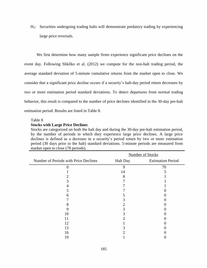
185
H3: Securities undergoing trading halts will demonstrate predatory trading by experiencing
large price reversals.
We first determine how many sample firms experience significant price declines on the
event day. Following Shkilko et al. (2012) we compute for the non-halt trading period, the
average standard deviation of 5-minute cumulative returns from the market open to close. We
consider that a significant price decline occurs if a security’s halt-day period return decreases by
two or more estimation period standard deviations. To detect departures from normal trading
behavior, this result is compared to the number of price declines identified in the 30-day pre-halt
estimation period. Results are listed in Table 8.
Table 8
Stocks with Large Price Declines Stocks are categorized on both the halt day and during the 30-day pre-halt estimation period,
by the number of periods in which they experience large price declines. A large price
declines is defined as a decrease in a security’s period return by two or more estimation
period (30 days prior to the halt) standard deviations. 5-minute periods are measured from
market open to close (78 periods).
Number of Stocks
Number of Periods with Price Declines Halt Day Estimation Period
0 9 70
1 14 5
2 8 1
3 7 1
4 7 1
5 7 0
6 5 0
7 3 0
8 2 0
9 3 0
10 3 0
11 2 0
12 1 0
13 3 0
16 2 0
19 1 0
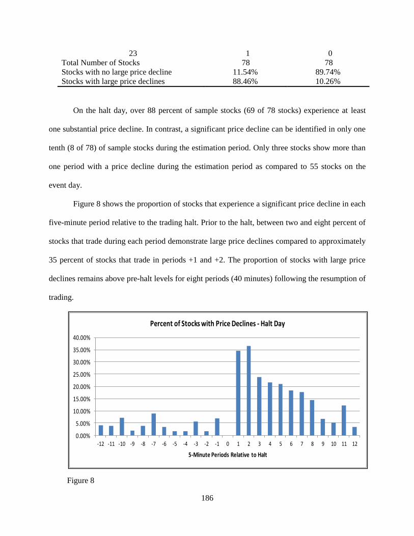
186
23 1 0
Total Number of Stocks 78 78
Stocks with no large price decline 11.54% 89.74%
Stocks with large price declines 88.46% 10.26%
On the halt day, over 88 percent of sample stocks (69 of 78 stocks) experience at least
one substantial price decline. In contrast, a significant price decline can be identified in only one
tenth (8 of 78) of sample stocks during the estimation period. Only three stocks show more than
one period with a price decline during the estimation period as compared to 55 stocks on the
event day.
Figure 8 shows the proportion of stocks that experience a significant price decline in each
five-minute period relative to the trading halt. Prior to the halt, between two and eight percent of
stocks that trade during each period demonstrate large price declines compared to approximately
35 percent of stocks that trade in periods +1 and +2. The proportion of stocks with large price
declines remains above pre-halt levels for eight periods (40 minutes) following the resumption of
trading.
Figure 8
0.00%
5.00%
10.00%
15.00%
20.00%
25.00%
30.00%
35.00%
40.00%
-12 -11 -10 -9 -8 -7 -6 -5 -4 -3 -2 -1 0 1 2 3 4 5 6 7 8 9 10 11 12
5-Minute Periods Relative to Halt
Percent of Stocks with Price Declines - Halt Day
187
Firms with Large Declines – by Period
The ratio of sample stocks with a large price decline to sample stocks that trade during each
period is computed. A large price declines is defined as a decrease in a security’s period
return by two or more estimation period (30 days prior to the halt) standard deviations. 5-
minute periods are measured backwards from the halt and forward from the resumption of
trade.
The high number of firms demonstrating large price declines immediately following the
continuation of trading suggests that the initial price behavior associated with predatory trading
is present for our sample stocks. However, these price declines could occur independently of
predation; it is necessary to examine the firms that exhibit substantial price declines and
determine if large price reversals occur. Borrowing from Shkilko et al. (2012), we identify a
large price reversal if the security’s return rebounds by 60 percent of the initial price decline by
the close of the trading day.
Of the 69 stocks that experience substantial price declines on the event day, 20 stocks,
representing 26 halts, evidence large price declines during periods +1 and +2. Only four of these
20 stocks demonstrate a large price reversal prior to the end of the trading day. In an attempt to
uncover differences in the return and short selling behavior of these four stocks as compared to
stocks that demonstrate substantial price declines in the first two post-halt periods but no
significant reversal, we compute, for each group, mean cumulative returns and abnormal short
selling levels for 12 post-halt periods. Abnormal short selling is the percentage difference
between shares sold short during the event period and the average daily number of shares sold
short during the estimation period. Results are shown in Figure 9, which makes a separate
comparison for each metric between reversal and non-reversal stocks. Figure 10 attempts to link
short selling behavior and returns; it displays these measurements together for each stock group.
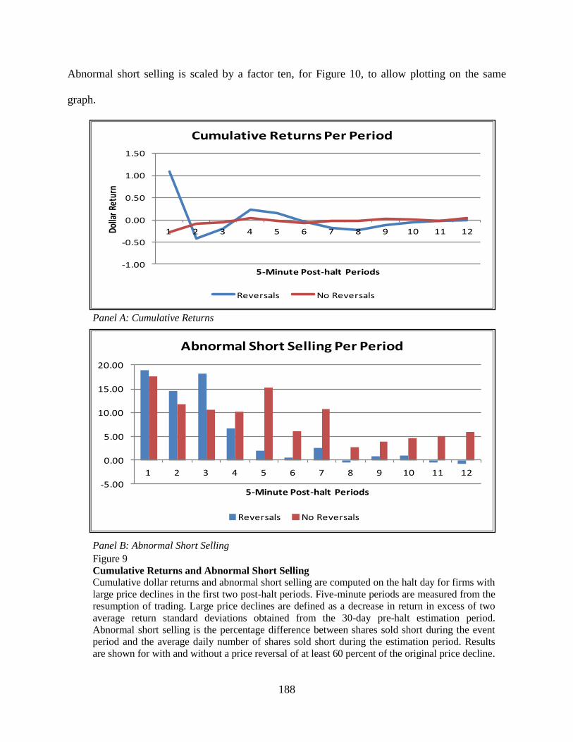
188
Abnormal short selling is scaled by a factor ten, for Figure 10, to allow plotting on the same
graph.
Panel A: Cumulative Returns
Panel B: Abnormal Short Selling
Figure 9
Cumulative Returns and Abnormal Short Selling
Cumulative dollar returns and abnormal short selling are computed on the halt day for firms with
large price declines in the first two post-halt periods. Five-minute periods are measured from the
resumption of trading. Large price declines are defined as a decrease in return in excess of two
average return standard deviations obtained from the 30-day pre-halt estimation period.
Abnormal short selling is the percentage difference between shares sold short during the event
period and the average daily number of shares sold short during the estimation period. Results
are shown for with and without a price reversal of at least 60 percent of the original price decline.
-1.00
-0.50
0.00
0.50
1.00
1.50
1 2 3 4 5 6 7 8 9 10 11 12Dolla
r Ret
urn
5-Minute Post-halt Periods
Cumulative Returns Per Period
Reversals No Reversals
-5.00
0.00
5.00
10.00
15.00
20.00
1 2 3 4 5 6 7 8 9 10 11 12
5-Minute Post-halt Periods
Abnormal Short Selling Per Period
Reversals No Reversals
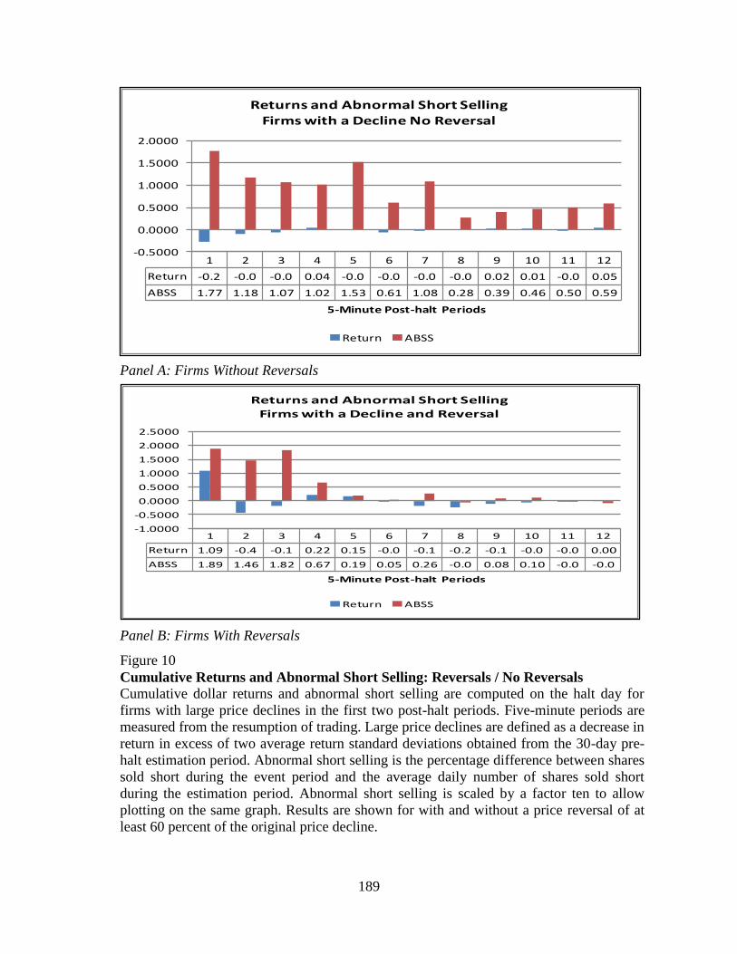
189
Panel A: Firms Without Reversals
Panel B: Firms With Reversals
Figure 10
Cumulative Returns and Abnormal Short Selling: Reversals / No Reversals
Cumulative dollar returns and abnormal short selling are computed on the halt day for
firms with large price declines in the first two post-halt periods. Five-minute periods are
measured from the resumption of trading. Large price declines are defined as a decrease in
return in excess of two average return standard deviations obtained from the 30-day pre-
halt estimation period. Abnormal short selling is the percentage difference between shares
sold short during the event period and the average daily number of shares sold short
during the estimation period. Abnormal short selling is scaled by a factor ten to allow
plotting on the same graph. Results are shown for with and without a price reversal of at
least 60 percent of the original price decline.
1 2 3 4 5 6 7 8 9 10 11 12
Return -0.2 -0.0 -0.0 0.04 -0.0 -0.0 -0.0 -0.0 0.02 0.01 -0.0 0.05
ABSS 1.77 1.18 1.07 1.02 1.53 0.61 1.08 0.28 0.39 0.46 0.50 0.59
-0.5000
0.0000
0.5000
1.0000
1.5000
2.0000
5-Minute Post-halt Periods
Returns and Abnormal Short Selling
Firms with a Decline No Reversal
Return ABSS
1 2 3 4 5 6 7 8 9 10 11 12
Return 1.09 -0.4 -0.1 0.22 0.15 -0.0 -0.1 -0.2 -0.1 -0.0 -0.0 0.00
ABSS 1.89 1.46 1.82 0.67 0.19 0.05 0.26 -0.0 0.08 0.10 -0.0 -0.0
-1.0000
-0.5000
0.0000
0.5000
1.0000
1.5000
2.0000
2.5000
5-Minute Post-halt Periods
Returns and Abnormal Short Selling
Firms with a Decline and Reversal
Return ABSS
190
From Figure 9, we make two noteworthy observations. Return patterns, shown in Panel
A, are quite different for each set of firms. The firms with price reversals demonstrate a
pronounced decline from periods +1 to +2, and a sharp rebound in periods +3 and +4. In
contrast, the non-reversing firms appear to have a gradual appreciation in price during the first
four post-halt periods without evidence of extreme price movements. Abnormal short selling
levels, shown in Panel B, suggest differences as well. Although levels are similar for both groups
immediately upon the resumption of trading, short selling for the reversal stocks remains
elevated for three periods and then declines substantially with near estimation periods levels by
the eighth post-halt period. Short selling levels for the non-reversing stocks appear to be more
arbitrary and they remain noticeably elevated throughout the periods examined.
Figure 10 fails to demonstrate for either firm group, a predatory relation between short
selling levels and returns. For firms with no reversal identified (Panel A), the highest short
selling levels and lowest returns occur simultaneously in the first post-halt period. For firms
experiencing reversals, short selling levels are highest immediately preceding the substantial
price decline in period two. However, short selling remains elevated in the two periods that
follow, even as the price begins to rebound. This observation is consistent with Shkilko et al.
(2012), who find that prior to large price reversals; short selling increases as short sellers demand
liquidity instead of supply it.
Our examination of price reversals provides only limited support for Hypothesis 3. We
document reliable evidence that substantial price declines surrounding interruptions in trading
occur. However, beyond our observations that return and short selling patterns appear different
for stocks depending on whether they experience a large price reversal, we are unable to

191
establish that the price reversals associated with predatory activity take place for a significant
portion of our sample of stocks.
192
CONCLUSION
The model of predation developed by Brunnermeier and Pedersen (2005) describes a
distinct pattern of price behavior: an initial price decline is followed by a substantial reversal.
Our research intent is to discover if predatory activity occurs surrounding trading halts – if
strategic market participants take advantage of a distressed trader’s need to liquidate.
Our investigation identifies that overall, sample stocks experience a substantial decline in
price immediately following the resumption of trading; this decline appears on aggregate to
reverse itself by the end of the trading day. Results also demonstrate that short selling and returns
exert influence on each other, however, the impact of non-short volume on returns is not
established. Although an increase in trading, both short and non-short volume, is identified
surrounding our trading halt events, the anticipated shift in buying and selling activity is not
evidenced, perhaps due to the manner in which transactions, particularly short sales, are
classified. Price reversals are identified for a fraction of sample stocks, but our research is unable
to definitively demonstrate that predatory behavior occurs surrounding halts in trading.
Aitken and Dyl (1990), in their examination of stock behavior subsequent to large price
changes, find statistically significant reversals in price. They look to previous research to provide
possible explanations, which might apply to the price behavior of sample stocks in our study. For
example, De Bondt and Thaler (1985) suggest that irrationality might lead investors to place too
much emphasis on events and thereby make inaccurate forecasts. Brown, Harlow, and Tinic
(1988) purport that in an uncertain environment, information is not incorporated immediately
and investors overreact to what they perceive as bad news.

193
LIST OF REFERENCES

194
Acharya, Viral and Lasse Heje Pederson, 2005, Asset Pricing with Liquidity Risk, Journal of
Financial Economics, 77, 375 – 410.
Aitken, Allen and Edward Dyl, 1990, Price Reversals, Bid-Ask Spreads, and Market Efficiency,
The Journal of Financial and Quantitative Analysis, 25 (4), 535 – 547.
Asquith, Paul, Rebecca Oman, and Christopher Safaya, 2010, Short Sales and Trade
Classification Algorithms, Journal of Financial Markets, 13 (1), 157-173.
Attari, Mukarram, Antonio Mello, and Martin Ruckes, 2005, Arbitraging Arbitrageurs, The
Journal of Finance, 60, 2471 – 2511.
Brown, K. C., W. Van Harlow, and S. M. Tinic, Risk Aversion, Uncertain Information, and
Market Efficiency, Journal of Financial Economics, 22 (2), 355 – 385.
Brown, Philip, David Walsh, and Andrea Yuen, 1997, The Interaction Between Order Imbalance
and Stock Price, Pacific-Basin Financial Journal, 5 (5), 539-557.
Brunnermeier, Markus, and Lasse Heje Pedersen, 2005, Predatory Trading, The Journal of
Finance, 60 (4), 1825 – 1863.
Brunnermeier, Markus, and Lasse Heje Pedersen, 2009, Market Liquidity and Funding Liquidity,
Review of Financial Studies, 22 (6), 2201 – 2238.
Cai, Fang, 2003, Was There Front Running During the LTCM Crisis?, Board of Governors of
The Federal Reserve System International Finance Discussion Paper #758,
http://ssrn.com/abstract=385560
Carlin, Bruce, Migueal Lobo and S. Viswanthan, 2007, Episodic Liquidity Crises: Cooperative
and Predatory Trading, The Journal of Finance, 62 (5), 2235 – 2274.
Chakrabarty, Bidisha, Pamela Moulton, and Andriy Shkilko, 2012, Short Sales, Long Sales, and
the Lee-Ready Trade Classification Algorithm Revisited, Journal of Financial Markets,
http://dx.doi.org/10.1016/j.finmar.2012.01.001
Chordia, Tarun, and Avanidhar Subrahmanyam, 2002, Order Imbalance and Individual Stock
Returns: Theory and Evidence, Journal of Financial Economics, 72 (3), 485-518.
Chordia, Tarun, Richard Roll, and Avanidhar Subrahmanyam, 2002, Order Imbalance, Liquidity,
and Market Returns, Journal of Financial Economics, 65 (3), 111-130.
Christie, William, Shane Corwin, and Jeffrey Harris, 2002, Nasdaq Trading Halts: The Impact of
Market Mechanisms on Prices, Trading Activity, and Execution Costs, The Journal of
Finance, 57 (3), 1443 – 1478.
Christophe, Stephen, Michael Ferri, and James Angel, 2004, Short-Selling Prior to Earnings
Announcements, The Journal of Finance, 59 (4), 1845 – 1875.
Corwin, Shane, and Marc Lipson, 2000, Order Flow and Liquidity around NYSE Trading Halts,
The Journal of Finance, 55 (4), 1771 – 1801.

195
D’Avolio, 2002, The Market for Borrowing Stock, Journal of Financial Economics, 66, 271 –
306.
De Bondt, Werner, and Richard Thaler, Does the Stock Market Overreact, Journal of Finance,
14 ( ), 793-805.
Diether, Karl, Kuan-Hui Lee, and Ingrid Werner, 2009A, It’s SHO time! Short-Sale Price Tests
and Market Quality, The Journal of Finance, 64 (1), 37 – 73.
Diether, Karl, Kuan-Hui Lee, and Ingrid Werner, 2009B, Short-Sale Strategies and Return
Predictability, The Review of Financial Studies, 22 (2), 575 – 607.
Easley, David, Robert Engle, Maureen O’Hara, and Liuren Wu, 2008, Time-Varying Arrival
Rates of Informed and Uninformed Trades, Journal of Financial Econometrics, 6 (2), 171 –
207.
Goldstein, Michael, and Kenneth Kavajecz, 2004, Trading Strategies During Circuit Breakers
and Extreme Market Movements, Journal of Financial Markets, 7, 301 – 333.
Kim, Yong, and J. Jimmy Yang, 2004, What Makes Circuit Breakers Attractive to Financial
Markets? A Survey, Financial Markets, Institutions & Instruments, 13 (3), 109 – 146.
Kryzanowski, Lawrence, 1979, The Efficacy of Trading Suspensions: A Regulatory Action
Designed to Prevent the Exploitation of Monopoly Information, The Journal of Finance,
34 (5), 1187 – 1200.
Lee, Charles, and Mark Ready, 1991, Inferring Trade Direction from Intraday Data, The Journal
of Finance, 46 (2), 733 – 754.
Lee, Charles, Mark Ready, and Paul Seguin, 1994, Volume, Volatility, and New York Stock
Exchange Trading Halts, The Journal of Finance, 49 (1), 183 – 214.
Madura, Jeff, Nivine Richie, and Alan Tucker, 2006, Trading Halts and Price Discovery, Journal
of Financial Services Research, 30, 311 – 328.
Onayev, Zhan, and Vladimir Zdorovtsov, 2008, Predatory Trading around Russell
Reconstitution, Working Paper Series, http://ssrn.com/abstract=1101341
Pastor, Lubos, and Robert Stambaugh, 2001, Liquidity Risk and Expected Stock Returns,
Working Paper Series, http://www.nber.org/papers/w8462
Reed, Adam, 2007, Costly Short Selling and Stock Price Adjustments to Earnings
Announcements, Working Paper, Obtained from website:
http://www.nd.edu/~carecob/April%202007%20Conference/Costly%20Short%20Selling%20
and%20Stock%20Price%20Adjustment%20to%20Earnings%20Announcements.pdf
Schoeneborn, Torsten and Alexander Schied, 2009, Liquidation in the Face of Adversity: Stealth
Versus Sunshine Trading, http://ssrn.com/abstract=1007014
Shkilko, Andriy, Bonnie Van Ness, and Robert Van Ness, 2012, Aggressive Short Selling and
Intraday Price Pressures, Financial Management, 41 (12), 345 – 370.

196
Stowe, John, and Xuejing Xing, 2011, R2: Does it Matter for Firm Valuation?, The Financial
Review, 46 (2), 233 - 250.
Subrahmanyam, Avanidhar, 1994, Circuit Breakers and Market Volatility: A Theoretical
Perspective, The Journal of Finance, 49 (1), 237 – 254.
Wong, Woon, Matthew Chang, and Anthony Tu, 2009, Are Magnet Effects caused by
Uninformed Traders? Evidence from the Taiwan Stock Exchange, Pacific-Basin Finance
Journal, 17, 28 – 40.
Xing, Xuejing, and Rand Anderson, 2011, Stock Price Synchronicity and Public Firm-specific
Information, Journal of Financial Markets, 14 (2), 259 – 276.

197
LIST OF APPENDICES

198
APPENDIX: A
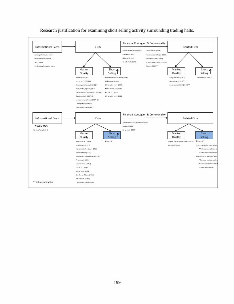
199
Research justification for examining short selling activity surrounding trading halts.
Kodres and Pritsker (2002) Chordia et al. (2000)
Earnings Announcements Kaufman (1994) Hasbrouck and Seppi (2001)
Dividend Declarations Alli et al. (1994) Subrahmanyam (1991)
Stock Splits Ghosh et al. (1998) Huberman and Halka (2001)
Bankruptcy Announcements Tookes (2008)**
Market
Quality
Short
Selling
Market
Quality
Short
Selling
Beaver (1968) {EA} Safieddine and Wilhelm (1996) Lang and Stulz (1992) Efendi et al. 2005 **
Lee et al. (1993) {EA} Aitken et al. (1998) Ferris et al. (1997) **
Aharony and Swary (1980) {D} Christophe et al. (2004) Bessler and Nohel (2000) **
Bajaj and Vijh (1995) {D} ** Karpoff and Lou (2010)
Datta and Iskandar-Datta (1995) {B} Blau et al. (2011)
Dawkins et al. (2007) {B} Christophe et al. (2010)
Lamoureux and Poon (1987) {SS}
Conroy et al. (1990) {SS}
Desai et al. (1998) {SS} **
Spiegel and Subrahmanyam (2000)
Trading Halts Tookes (2008)**
Kim and Yang (2004) Jiang et al. (2009)
Market
Quality
Short
Selling
Market
Quality
Short
Selling
Madura et al. (2006) Essay 1 Spiegel and Subrahmanyam (2000) Essay 2
Kyrzanowski (1979) Jian et al. (2009) Prior to a trading halt, securities for related firms will experience:
Howe and Schlarbaum (1986) * An increase in abnormal selling measures
Kim and Rhee (1997) * Increase in comovement in short selling measures
Kryzanowski and Nemiroff (1998) Related stocks with high short interest will evidence a larger:
Ferris et al. (1992) * Decrease in abnormal returns
Christie et al. (2002) * Increase in price volatility
Lee et al. (1994) * Increase in spreads
Bacha et al. (2008)
Engelen and Kabir (2006)
Hauser et al. (2006)
** Informed trading Corwin and Lipson (2000)
Informational Event
Financial Contagion & Commonality
Firm Related Firm
Informational Event Firm
Financial Contagion & Commonality
Related Firm

200
APPENDIX: B
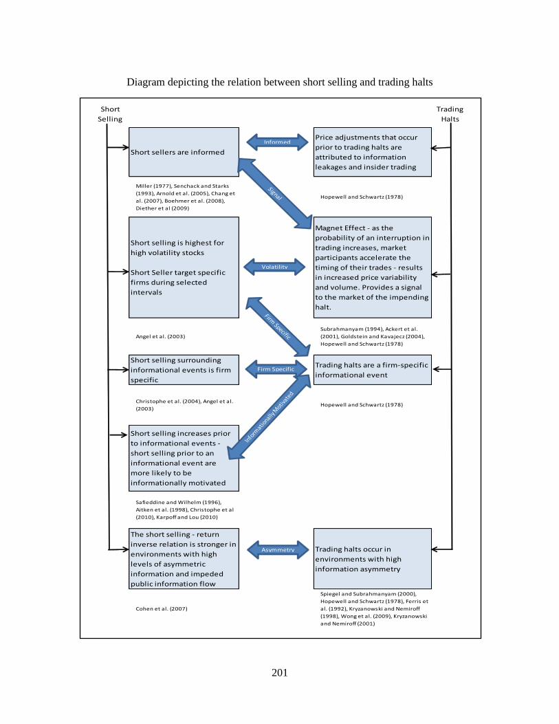
201
Diagram depicting the relation between short selling and trading halts
Short
Selling
Trading
Halts
Short sellers are informed
Price adjustments that occur
prior to trading halts are
attributed to information
leakages and insider trading
Miller (1977), Senchack and Starks
(1993), Arnold et al. (2005), Chang et
al. (2007), Boehmer et al. (2008),
Diether et al (2009)
Hopewell and Schwartz (1978)
Short selling is highest for
high volatility stocks
Short Seller target specific
firms during selected
intervals
Magnet Effect - as the
probability of an interruption in
trading increases, market
participants accelerate the
timing of their trades - results
in increased price variability
and volume. Provides a signal
to the market of the impending
halt.
Angel et al. (2003)
Subrahmanyam (1994), Ackert et al.
(2001), Goldstein and Kavajecz (2004),
Hopewell and Schwartz (1978)
Short selling surrounding
informational events is firm
specific
Trading halts are a firm-specific
informational event
Christophe et al. (2004), Angel et al.
(2003)Hopewell and Schwartz (1978)
Short selling increases prior
to informational events -
short selling prior to an
informational event are
more likely to be
informationally motivated
Safieddine and Wilhelm (1996),
Aitken et al. (1998), Christophe et al
(2010), Karpoff and Lou (2010)
The short selling - return
inverse relation is stronger in
environments with high
levels of asymmetric
information and impeded
public information flow
Trading halts occur in
environments with high
information asymmetry
Cohen et al. (2007)
Spiegel and Subrahmanyam (2000),
Hopewell and Schwartz (1978), Ferris et
al. (1992), Kryzanowski and Nemiroff
(1998), Wong et al. (2009), Kryzanowski
and Nemiroff (2001)
Informed
Volatility
Asymmetry
Firm Specific

202
APPENDIX: C
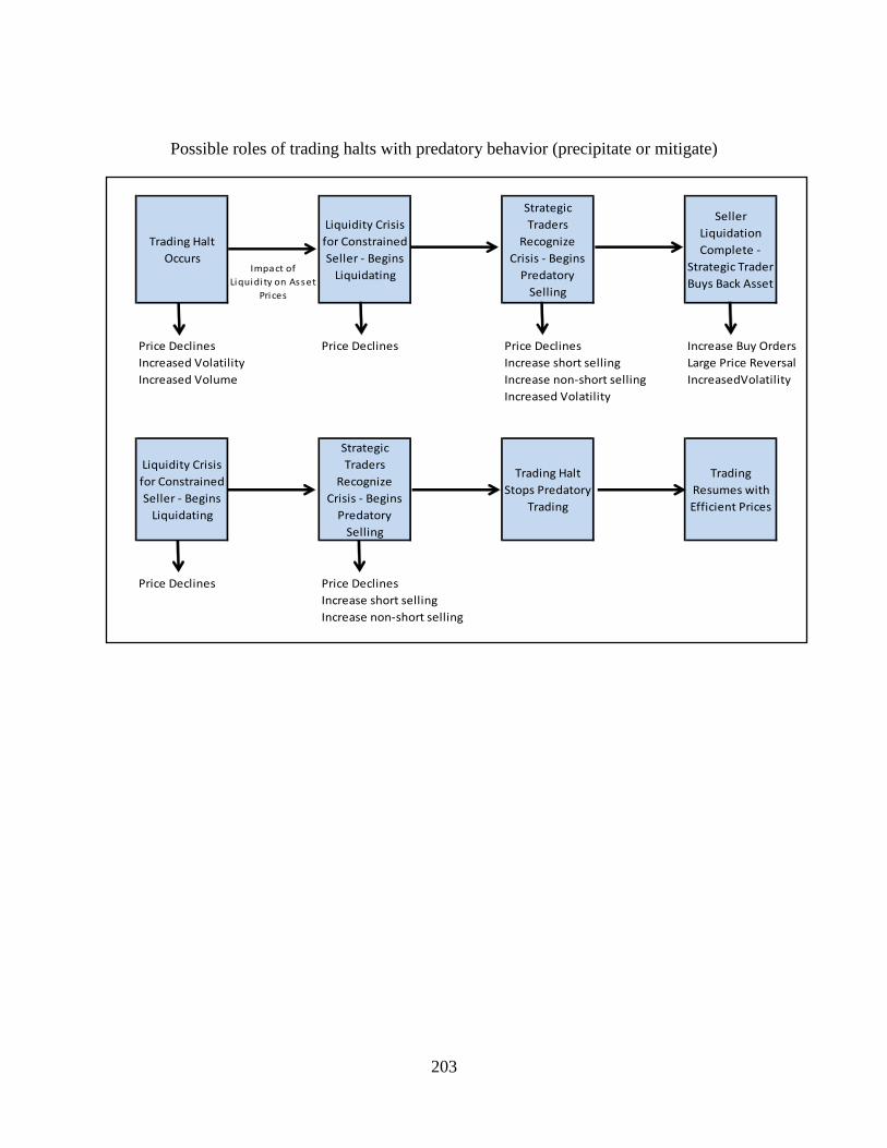
203
Possible roles of trading halts with predatory behavior (precipitate or mitigate)
Trading Halt
OccursImpact of
Liquidi ty on Asset
Prices
Liquidity Crisis
for Constrained
Seller - Begins
Liquidating
Strategic
Traders
Recognize
Crisis - Begins
Predatory
Selling
Seller
Liquidation
Complete -
Strategic Trader
Buys Back Asset
Price Declines Price Declines Price Declines Increase Buy Orders
Increased Volatility Increase short selling Large Price Reversal
Increased Volume Increase non-short selling IncreasedVolatility
Increased Volatility
Liquidity Crisis
for Constrained
Seller - Begins
Liquidating
Strategic
Traders
Recognize
Crisis - Begins
Predatory
Selling
Trading Halt
Stops Predatory
Trading
Trading
Resumes with
Efficient Prices
Price Declines Price Declines
Increase short selling
Increase non-short selling

204
APPENDIX D
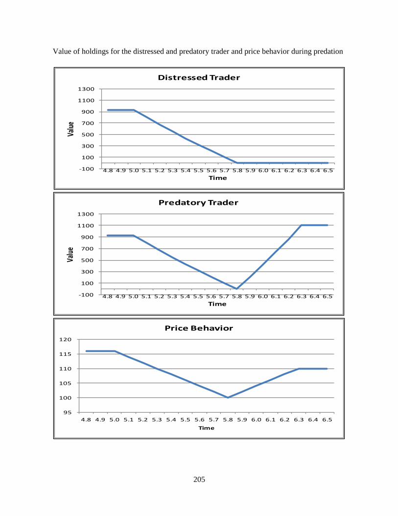
205
Value of holdings for the distressed and predatory trader and price behavior during predation
-100
100
300
500
700
900
1100
1300
4.8 4.9 5.0 5.1 5.2 5.3 5.4 5.5 5.6 5.7 5.8 5.9 6.0 6.1 6.2 6.3 6.4 6.5
Valu
e
Time
Distressed Trader
-100
100
300
500
700
900
1100
1300
4.8 4.9 5.0 5.1 5.2 5.3 5.4 5.5 5.6 5.7 5.8 5.9 6.0 6.1 6.2 6.3 6.4 6.5
Valu
e
Time
Predatory Trader
95
100
105
110
115
120
4.8 4.9 5.0 5.1 5.2 5.3 5.4 5.5 5.6 5.7 5.8 5.9 6.0 6.1 6.2 6.3 6.4 6.5
Time
Price Behavior

206
APPENDIX E

207
List of Sample Firms
Firm Symbol Mode SIC
AMERICREDIT CORP ACF 4 Personal Credit Institutions
ADAMS RESOURCES & ENERGY INC AE 7 Crude Petroleum & Natural Gas
UNITED CAPITAL CORP AFP 11 Electronic Coils, Transformers & Other Inductors
AGRIUM INC AGU 11 Agricultural Chemicals
AMERICAN ISRAELI PAPER MLS LTD AIP 11 Paper Mills
ALPHARMA INC ALO 11 Pharmaceutical Preparations
BLAIR CORP BL 4 Retail-Catalog & Mail-Order Houses
BAUSCH & LOMB INC BOL 11 Retail-Building Materials, Hardware, Garden Supply
CONAGRA INC CAG 11 Meat Packing Plants
CAMBREX CORP CBM 11 Services-Engineering, Accounting, Research, Management
CAMECO CORP CCJ 11 Miscellaneous Metal Ores
CORUS ENTERTAINMENT INC CJR 11 Radio Broadcasting Stations
CORUS ENTERTAINMENT INC CJR 11 Radio Broadcasting Stations
CORUS ENTERTAINMENT INC CJR 11 Radio Broadcasting Stations
CANTEL MEDICAL CORP CMN 11 Services-Commercial Physical & Biological Research
CAREMARK RX INC CMX 11 Services-Home Health Care Services
CANADIAN NATIONAL RAILWAY CO CNI 11 Railroads, Line-Haul Operating
COMSTOCK RESOURCES INC CRK 11 Crude Petroleum & Natural Gas
CONTINENTAL MATERIALS CORP CUO 11 Concrete, Gypsum & Plaster Products
C V S CORP CVS 11 Retail-Drug Stores and Proprietary Stores
DELUXE CORP DLX 11 Blankbooks, Looseleaf Binders & Bookbindg & Related Work
DOMTAR INC DTC 11 Paper Mills
DYNEGY INC NEW DYN 11 Natural Gas Transmission
ENCANA CORP ECA 11 Crude Petroleum & Natural Gas
ELKCORP ELK 11 Asphalt Paving & Roofing Materials
ENERGY PARTNERS LTD EPL 11 Crude Petroleum & Natural Gas
EMPIRE RESOURCES INC DEL ERS 7 Wholesale-Metals Service Centers & of fices
FAIRCHILD SEMICONDUCTOR INTL INC FCS 11 Semiconductors & Related Devices
FORDING CANADIAN COAL TRUST FDG 11 Trust Services
FAMILY DOLLAR STORES INC FDO 11 Retail-Variety Stores
HALLWOOD GROUP INC HWG 11 Broadwoven Fabric Mills, Man Made Fiber & Silk
IAMGOLD CORP IAG 11 Gold and Silver Ores
IRWIN FINANCIAL CORP IFC 4 State Commercial Banks
IMERGENT INC IIG 7 Services-Computer Integrated Systems Design
QUEBECOR WORLD INC IQW 11 Commercial Printing
INTERTAPE POLYMER GROUP INC ITP 11 Converted Paper & Paperboard Prods (No Containers/Boxes)
J E D OIL INC JDO 11 Crude Petroleum & Natural Gas
JONES APPAREL GROUP INC JNY 11 Apparel & Other Finished Prods of Fabrics & Similar Matl
KADANT INC KAI 11 Special Industry Machinery (No Metalworking Machinery)
LEVITT CORP FLA LEV 11 Land Subdividers & Developers (No Cemeteries)
LIONS GATE ENTERTAINMENT CORP LGF 11 Services-Motion Picture & Video Tape Production
MINERALS TECHNOLOGIES INC MTX 11 Industrial Inorganic Chemicals
NAVISTAR INTERNATIONAL CORP NAV 11 Truck & Bus Bodies
NAVISTAR INTERNATIONAL CORP NAV 11 Truck & Bus Bodies
NACCO INDUSTRIES INC NC 11 Industrial Trucks, Tractors, Trailers & Stackers
NOVAGOLD RESOURCES INC NG 11 Gold and Silver Ores
NUVEEN MASS DIV ADV MUNI FD NMB 7 Trust Services
NATIONAL SEMICONDUCTOR CORP NSM 11 Semiconductors & Related Devices
NATIONAL SEMICONDUCTOR CORP NSM 11 Semiconductors & Related Devices
NATIONAL SEMICONDUCTOR CORP NSM 11 Semiconductors & Related Devices
NATIONAL SEMICONDUCTOR CORP NSM 11 Semiconductors & Related Devices
NATIONAL SEMICONDUCTOR CORP NSM 11 Semiconductors & Related Devices
QUANEX CORP NX 11 Steel Works, Blast Furnaces & Rolling Mills (Coke Ovens)
ONE LIBERTY PROPERTIES INC OLP 11 Real Estate Investment Trusts
PIONEER DRILLING CO PDC 7 Drilling Oil & Gas Wells
PARK NATIONAL CORP PRK 7 National Commercial Banks

208
RIVIERA HOLDINGS CORP RIV 11 Services-Miscellaneous Amusement & Recreation
RETAIL HOLDRS TRUST RTH 4 Trust Services
BOSTON BEER INC SAM 11 Malt Beverages
BOSTON BEER INC SAM 11 Malt Beverages
BOSTON BEER INC SAM 11 Malt Beverages
BOSTON BEER INC SAM 11 Malt Beverages
SCHWAB CHARLES CORP NEW SCH 11 Security Brokers, Dealers & Flotation Companies
SHAW GROUP INC SGR 11 Miscellaneous Fabricated Metal Products
STONE ENERGY CORP SGY 11 Crude Petroleum & Natural Gas
SIGNET GROUP PLC SIG 11 Retail-Jewelry Stores
SUNLINK HEALTH SYSTEMS INC SSY 11 Services-Commercial Physical & Biological Research
TELEPHONE & DATA SYSTEMS INC TDS 4 Radiotelephone Communications
TEKTRONIX INC TEK 11 Instruments For Meas & Testing of Electricity & Elec Signals
TENET HEALTHCARE CORP THC 11 Services-General Medical & Surgical Hospitals, NEC
TODCO THE 11 Drilling Oil & Gas Wells
TECHNICAL OLYMPIC U S A INC TOA 11 General Bldg Contractors - Residential Bldgs
TELUS CORP TU 11 Radiotelephone Communications
UNITEDHEALTH GROUP INC UNH 11 Hospital & Medical Service Plans
UNISOURCE ENERGY CORP UNS 11 Electric Services
UNITED STATES CELLULAR CORP USM 4 Radiotelephone Communications
WESTMORELAND COAL CO WLB 7 Bituminous Coal & Lignite Mining
WELLSFORD REAL PROPERTIES INC WRP 11 Real Estate Investment Trusts

209
VITA
Mary C. Funck
Academic Background
M.B.A. Western Illinois University Macomb, IL Finance 2006
M.S. Western Illinois University Macomb, IL Computer Science 2002
B.S. Western Illinois University Macomb, IL Computer Science 1997
Work Experience
Academic Experience
Graduate Teaching and Research Assistant, University of Mississippi (2007 – 2012).
Department of Finance.
Senior Associate Faculty, Western Illinois University (1998 – 2007). Computer Science
Department.
Faculty Presenter, Western Illinois University (Summer 2006). Center of Innovation, Research,
and Teaching.
Administrative Intern, Western Illinois University (2004 – 2005). Western Illinois
Entrepreneurship Center.
Graduate Teaching Assistant, Western Illinois University (Spring Semester 1998). Computer
Science Department.
Teaching
Courses Taught
FIN 331 Business Finance I (taught for 11 semesters)
FIN 334 Investments (taught for 2 semesters)
CS 101 Introduction to Computers (Computer Applications and Literacy)
CS 301 Advanced Spreadsheet Concepts (Microsoft Excel)
CS 483(G) Micro Database Applications (Microsoft Access)
CS 220 Introduction to COBOL (IBM Mainframe Platform)

210
CS 230 External Files (Intermediate COBOL & JCL)
CS 211 Principles of Computer Science I (Introductory Computer Science Principles)
CS 214 Principles of Computer Science II (Introductory Java Programming)
Research / Intellectual Contributions
Publications
Watson, E., and Funck, M. (2012). “A Cloudy Day in the Market: Short Selling Behavioral
Bias or Trading Strategy,” International Journal of Managerial Finance, 8 (3), 238 – 255.
Papers Under Review
Funck, M, Van Ness B.F., and Van Ness, R. A. (2012). “Fly the Friendly Skynet: Reaction to a
False-News Event for United Airlines,” forthcoming publication at the Journal of Applied
Finance.
Presentation of Papers
Funck, M, Van Ness B.F., and Van Ness, R. A. (2011). “United Airlines and an Internet Bot:
Market Quality, Trading Halts and Investor Reaction to a No-News Event,” presented at the
Eastern Finance Association Meeting, Savannah, Georgia, April 2011.
Myers, J., Horstman (Funck) M., Marchand, H., “Methamphetamine Precursor Control Act
(MPCA) Study .” presented at i2 National User Conference, Arlington, VA, May 2007.
Horstman (Funck) M., Myers, J., Marchand, H., “Methamphetamine Precursor Control Act
(MPCA) Study.” Presented at the Illinois State Academy of Science 2007 Annual Meeting.
Springfield, IL, April 2007.
Horstman (Funck) M., Brown J., Myers, J., “A New Tool, Using Alice to Overcome Obstacles
Inherent in Teaching Introductory Programming Concepts.” Presented at the Illinois State
Academy of Science 2007 Annual Meeting. Springfield, IL, April 2007.
Hackmann, R., Horstman (Funck) M., Sawhney, S., Agan, Y., “Information Value of
Secondary Statistics.” Presented at the Midwest Business Administration Association Annual
Meeting, Chicago, IL March 2007.
Marchand, H., Myers, J., Horstman (Funck) M., “Methamphetamine Precursor Control Act
(MPCA) Study.” Presented at the third Annual Rural Public Health Institute, Effingham, IL,

211
March 2007.
Hackmann, R., Horstman (Funck) M., “Disparate U.S. GDP Values and their Implication in a
Global Economy.” American Association of Business and Behavioral Sciences Annual
Meeting, Las Vegas, NV, February 2007.
Sawhney, R., Horstman (Funck) M., “Examining Patient Record Flow at CS Medical Center.”
American Association of Business and Behavioral Sciences Annual Meeting, Las Vegas, NV,
February 2007.
Horstman (Funck), M., "Entrepreneurship – An Innovative Approach to Product Availability in
Rural Retail Markets.” Midwest Business Administration Association Annual Meeting,
Chicago, IL, March 2005.
Research Grants
Internally Funded
2009 Funck, M. Graduate Summer Research Grant, University of Mississippi
2006 Myers, J., Horstman (Funck), M., Marchand, H., Internal Grant -
Methamphetamine Precursor Control Act (MPCA) Study, Western Illinois
University
Service
Service to the University
Departmental Activity
Coordinator of Graduate Teaching Assistants, Western Illinois University, Computer Science
Department 1999 – 2004
Chair, Service Course Committee, Western Illinois University, Computer Science
Department
College Activity
Proctor – Bloomberg Assessment Test, School of Business Administration, University of
Mississippi, November 2011

212
University –Wide Activity
Served in the Faculty Mentor Program – Western Illinois University
Served as faculty participant in student orientation programs – Western Illinois University
Service to the Profession
Editorial and Review Activities
2011 Invited Manuscript Contributor, Brigham Houston, “Fundamentals of
Financial Management” seventh edition
2009 Invited reviewer for journal article submission to The Financial Review
(National)
2007 Invited Manuscript Reviewer, Pearson Education “Exploring Series”
2005 Invited Manuscript Reviewer, “Java Programming – From Problem Analysis
to Program Design”, Chapters 15 - 20
2004 – 2005 Invited Manuscript Reviewer, "Java Programming - From Problem Analysis
to Program Design."
2004 Invited Manuscript Reviewer, "Robots: Learning to program with Java."
2004 Invited Manuscript Reviewer, comparison of three Java texts for Course
Technology Publishers
2003 – 2004 Invited Manuscript Reviewer, "Go! Series."
2002 – 2003 Invited Manuscript Reviewer, "Computing Today."
2002 Invited Manuscript Reviewer, "Essentials Series."
2002 Invited Manuscript Reviewer, "Grauer Exploring Series."
Other
Awards
2011 ‘Random Acts of Kindness’ award from Student Alumni Council, University
of Mississippi
1998 Outstanding Graduate Teaching Assistant, Computer Science Department,
Western Illinois University