INVITED P A P E R Fundamentalsof … · P A P E R Fundamentalsof FastSimulationAlgorithms forRFCircuits The newest generationof circuit simulators perform periodic steady-state analysis

INV ITEDP A P E R

Fundamentals ofFast Simulation Algorithmsfor RF CircuitsThe newest generation of circuit simulators perform periodic steady-state analysis ofRF circuits containing thousands of devices using a variety of matrix-implicittechniques which share a common analytical framework.

By Ognen Nastov, Rircardo Telichevesky, Member IEEE,

Ken Kundert, and Jacob White, Member IEEE

ABSTRACT | Designers of RF circuits such as power amplifiers,

mixers, and filters make extensive use of simulation tools

which perform periodic steady-state analysis and its exten-

sions, but until the mid 1990s, the computational costs of these

simulation tools restricted designers from simulating the

behavior of complete RF subsystems. The introduction of fast

matrix-implicit iterative algorithms completely changed this

situation, and extensions of these fast methods are providing

tools which can perform periodic, quasi-periodic, and periodic

noise analysis of circuits with thousands of devices. Even

though there are a number of research groups continuing to

develop extensions of matrix-implicit methods, there is still no

compact characterization which introduces the novice re-

searcher to the fundamental issues. In this paper, we examine

the basic periodic steady-state problem and provide both

examples and linear algebra abstractions to demonstrate

connections between seemingly dissimilar methods and to try

to provide a more general framework for fast methods than the

standard time-versus-frequency domain characterization of

finite-difference, basis-collocation, and shooting methods.

KEYWORDS | Circuit simulation; computer-aided analysis; design

automation; frequency-domain analysis; numerical analysis

I . INTRODUCTION

The intensifying demand for very high performanceportable communication systems has greatly expandedthe need for simulation algorithms that can be used toefficiently and accurately analyze frequency response,distortion, and noise of RF communication circuits such asmixers, switched-capacitor filters, and amplifiers. Al-though methods like multitone harmonic balance, lineartime-varying, and mixed frequency-time techniques [4],[6]–[8], [26], [37] can perform these analyses, thecomputation cost of the earliest implementations of thesetechniques grew so rapidly with increasing circuit size thatthey were too computationally expensive to use for morecomplicated circuits. Over the past decade, algorithmicdevelopments based on preconditioned matrix-implicitKrylov-subspace iterative methods have dramaticallychanged the situation, and there are now tools which caneasily analyze circuits with thousands of devices. Precondi-tioned iterative techniques have been used to accelerateperiodic steady-state analysis based on harmonic balancemethods [5], [11], [30], time-domain shooting methods[13], and basis-collocation schemes [41]. Additional resultsfor more general analyses appear constantly.

Though there are numerous excellent surveys onanalysis technques for RF circuits [23], [35], [36], [42],the literature analyzing the fundmentals of fast methods islimited [40], making it difficult for novice researchers tocontribute to the field. In this paper, we try to provide acomprehensive yet approachable presentation of fast

Manuscript received May 23, 2006; revised August 27, 2006. This work was originallysupported by the DARPA MAFET program, and subsequently supported by grantsfrom the National Science Foundation, in part by the MARCO Interconnect FocusCenter, and in part by the Semiconductor Research Center.O. Nastov is with Agilent Technologies, Inc., Westlake Village, CA 91362 USA(e-mail: [email protected]).R. Telichevesky is with Kineret Design Automation, Inc., Santa Clara, CA 95054 USA(e-mail: [email protected]).K. Kundert is with Designer’s Guide Consulting, Inc., Los Altos, CA 94022 USA(e-mail: [email protected]).J. White is with the Research Laboratory of Electronics and Department of ElectricalEngineering and Computer Science, Massachusetts Institute of Technology,Cambridge, MA 02139 USA (e-mail: [email protected]).

Digital Object Identifier: 10.1109/JPROC.2006.889366

600 Proceedings of the IEEE | Vol. 95, No. 3, March 2007 0018-9219/$25.00 !2007 IEEE

methods for periodic steady-state analysis by combiningspecific examples with clarifying linear algebra abstrac-tions. Using these abstractions, we can demonstrate theclear connections between finite-difference, shooting,harmonic balance, and basis-collocation methods forsolving steady-state problems. For example, among usersof circuit simulation programs, it is common to categorizenumerical techniques for computing periodic steady-stateas either time-domain (finite-difference) or frequency-domain (harmonic balance), but the use of Kroneckerproduct representations in this paper will make clear thatnone of the fast methods for periodic steady-statefundamentally rely on properties of a Fourier series.

We start, in the next section, by describing thedifferent approaches for fomulating steady-state problemsand then present the standard numerical techniques in amore general framework that relies heavily on theKronecker product representation. Fast methods aredescribed in Section IV, along with some analysis andcomputational results. And as is common practice, we endwith conclusions and acknowledgements.

II . PERIODIC STEADY STATE

As an example of periodic steady state analysis, considerthe RLC circuit shown in Fig. 1. If the current source inFig. 1 is a sinusoid, and the initial capacitor voltage andinductor current are both zero, then the capacitor voltagewill behave as shown in Fig. 2. As the figure shows, theresponse of the circuit is a sinusoid whose amplitude growsuntil achieving a periodically repeating steady state. Thesolution plotted in Fig. 2 is the result of a numericalsimulation, and each of the many small circles in the plotcorresponds to a simulation timestep. Notice that a verylarge number of timesteps are needed to compute thissolution because of the many oscillation cycles before thesolution builds up to a steady state.

For this simple RLC circuit, it is possible to avoid themany timestep simulation and directly compute thesinusoidal steady state using what is sometimes referredto as phasor analysis [2]. To use phasor analysis, first recallthat the time behavior of the capacitor voltage for such anRLC circuit satisfies the differential equation

d2vc!t"dt2

# 1

rc

dv!t"dt

# 1

lcv!t" # di!t"

dt$ 0: (1)

Then, since a cosinusoidal input current is the real part of acomplex exponential, Ioej!t where j $

!!!!!!

%1p

, in sinusoidalsteady state the voltage must also be the real part of acomplex exponential given by

v!t" $ Realj!

%!2 # 1rc!# 1

lc

Ioej!t

" #

(2)

as can be seen by substituting v!t" $ Voej!t in (1) andsolving for Vo.

The simple phasor analysis used above for computingsinusoidal steady is not easily generalized to nonlinearcircuits, such as those with diodes and transistors. Thebehavior of such nonlinear circuits may repeat periodicallyin time given a periodic input, but that periodic responsewill almost certainly not be a sinusoid. However, there areapproaches for formulating systems of equations that canbe used to compute directly the periodic steady state of agiven nonlinear circuit, avoiding the many cycle timeintegration shown in Fig. 2. In the next subsection, webriefly describe one standard form for generating systemsof differential equations from circuits, and the subsectionsthat follow describe two periodic steady-state equationformulations, one based on replacing the differentialequation initial condition with a boundary condition andthe second based on using the abstract idea of a statetransition function. In later sections, we will describe

Fig. 1. Parallel resistor, capacitor, and inductor (RLC) circuit with

current source input.

Fig. 2. Transient behavior of RLC circuit with R $ 30, C $ 1, L $ 1,

and is!t" $ cos t.

Nastov et al. : Fundamentals of Fast Simulation Algorithms for RF Circuits

Vol. 95, No. 3, March 2007 | Proceedings of the IEEE 601

several numerical techniques for solving these twoformulations of the periodic steady-state problem.

A. Circuit Differential EquationsIn order to describe a circuit to a simulation program, one

must specify both the topology, how the circuit elements areinterconnected, and the element constitutive equations, howthe element terminal currents and terminal voltages arerelated. The interconnection can be specified by labelingn# 1 connection points of element terminals, referred to asthe nodes, and then listing which of b element terminals areconnected to which node. A system of n equations in bunknowns is then generated by insisting that the terminalcurrents incident at each node, except for a reference orBground[ node, sum to zero. This conservation law equationis usually referred to as the Kirchhoff current law (KCL). Inorder to generate a complete system, the element constitu-tive equations are used to relate the n node voltages withrespect to ground to b element terminal currents. The resultis a system of n# b equations in n# b variables, thevariables being ground-referenced node voltages and termi-nal currents. For most circuit elements, the constitutiveequations are written in a voltage-controlled form, meaningthat the terminal currents are explicit functions of terminalvoltages. The voltage-controlled constitutive equations canbe used to eliminate most of the unknown branch currents inthe KCL equation, generating a system of equations withmostly ground-referenced node voltages as unknowns. Thisapproach to generating a system of equations is referred to asmodified nodal analysis and is the equation formulationmostcommonly used in circuit simulation programs [1], [3].

For circuits with energy storage elements, such asinductors and capacitors, the constitutive equations in-clude time derivatives, so modified nodal analysis gen-erates a system of N differential equations in N variables ofthe form

d

dtq v!t"! " # i v!t"! " # u!t" $ 0 (3)

where t denotes time, u!t" is a N-length vector of giveninputs, v is an N-length vector of ground-referenced nodevoltages and possibly several terminal currents, i!&" is afunction that maps the vector of N mostly node voltages toa vector of N entries most of which are sums of resistivecurrents at a node, and q!&" is a function which maps thevector of N mostly node voltages to a vector of N entriesthat are mostly sums of capacitive charges or inductivefluxes at a node.

If the element constitutive equations are linear, or arelinearized, then (3) can be rewritten in matrix form

Cd

dtv!t" # Gv!t" # u!t" $ 0 (4)

where C and G are each N ' N matrices whose elementsare given by

Cj;k $@qj@vk

Gj;k $@ij@vk

: (5)

The basic forms given in (3) and (4) will be usedextensively throughout the rest of this paper, so to make theideas clearer, consider the example of the current-sourcedriven RLC circuit given in Fig. 1. The differential equationsystem generated by modified nodal analysis is given by

c 00 l

$ %

d

dtvc!t"il!t"

$ %

#1r 1%1 0

$ %

vc!t"il!t"

$ %

# is!t"0

$ %

$0 (6)

where vc!t" is the voltage across the capacitor, il!t" is thecurrent through the inductor, and is!t" is the sourcecurrent.

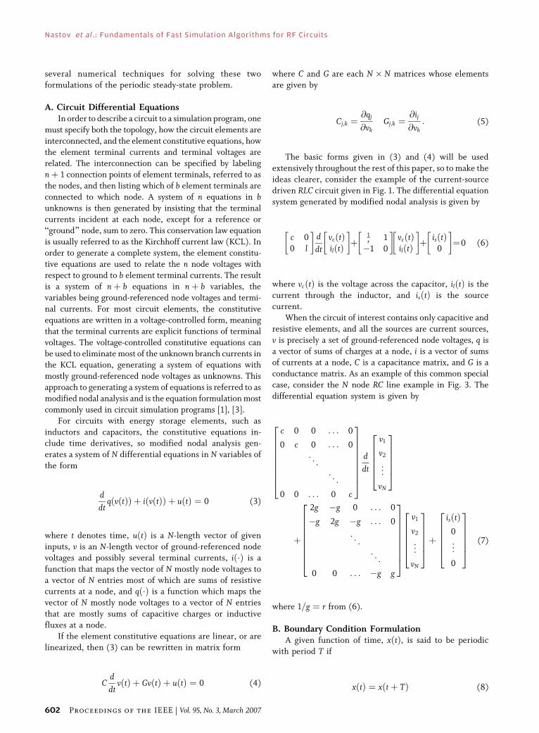
When the circuit of interest contains only capacitive andresistive elements, and all the sources are current sources,v is precisely a set of ground-referenced node voltages, q isa vector of sums of charges at a node, i is a vector of sumsof currents at a node, C is a capacitance matrix, and G is aconductance matrix. As an example of this common specialcase, consider the N node RC line example in Fig. 3. Thedifferential equation system is given by

c 0 0 . . . 0

0 c 0 . . . 0

. ..

. ..

0 0 . . . 0 c

2

6

6

6

6

6

6

6

4

3

7

7

7

7

7

7

7

5

d

dt

v1

v2

..

.

vN

2

6

6

6

6

4

3

7

7

7

7

5

#

2g %g 0 . . . 0

%g 2g %g . . . 0

. ..

. ..

0 0 . . . %g g

2

6

6

6

6

6

6

6

4

3

7

7

7

7

7

7

7

5

v1

v2

..

.

vN

2

6

6

6

6

4

3

7

7

7

7

5

#

is!t"0

..

.

0

2

6

6

6

6

4

3

7

7

7

7

5

(7)

where 1=g $ r from (6).

B. Boundary Condition FormulationA given function of time, x!t", is said to be periodic

with period T if

x!t" $ x!t# T" (8)


602 Proceedings of the IEEE | Vol. 95, No. 3, March 2007

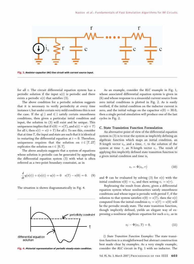
for all t. The circuit differential equation system has aperiodic solution if the input u!t" is periodic and thereexists a periodic v!t" that satisfies (3).

The above condition for a periodic solution suggeststhat it is necessary to verify periodicity at every timeinstance t, but under certain very mild conditions this is notthe case. If the q!&" and i!&" satisfy certain smoothnessconditions, then given a particular intial condition andinput, the solution to (3) will exist and be unique. Thisuniqueness implies that if v!0" $ v!T", and u!t" $ u!t# T"for all t, then v!t" $ v!t# T" for all t. To see this, considerthat at time T, the input and state are such that it is identicalto restarting the differential equation at t $ 0. Therefore,uniqueness requires that the solution on t 2 (T; 2T)replicates the solution on t 2 (0; T).

The above analysis suggests that a system of equationswhose solution is periodic can be generated by appendingthe differential equation system (3) with what is oftenreferred as a two-point boundary constraint, as in

d

dtq v!t"! " # i v!t"! " # u!t" $ 0 v!T" % v!0" $ 0: (9)

The situation is shown diagrammatically in Fig. 4.

As an example, consider the RLC example in Fig. 1,whose associated differential equation system is given in(6) and whose response to a sinusoidal current source fromzero initial conditions is plotted in Fig. 2. As is easilyverified, if the initial condition on the inductor current iszero, and the initial voltage on the capacitor v!0" $ 30:0,then a single period simulation will produce one of the lastcycles in Fig. 2.

C. State Transistion Function FormulationAn alternative point of view of the differential equation

system in (3) is to treat the system as implicitly defining analgebraic function which maps an initial condition, anN-length vector vo, and a time, ! , to the solution of thesystem at time ! , an N-length vector v! . The result ofapplying this implicitly defined state transition function toa given initial condition and time is,

v! $ !!vo; !" (10)

and ! can be evaluated by solving (3) for v!t" with theinitial condition v!0" $ vo, and then setting v! $ v!!".

Rephrasing the result from above, given a differentialequation system whose nonlinearities satisfy smoothnessconditions and whose input is periodic with period T, if thesolution to that system satisfies v!0" $ v!T", then the v!t"computed from the initial condition vT $ v!T" $ v!0" willbe the periodic steady state. The state transition function,though implicitly defined, yields an elegant way of ex-pressing a nonlinear algebraic equation for such a vT , as in

vT % !!vT; T" $ 0: (11)

1) State Transition Function Examples: The state transi-tion function is a straightforward but abstract constructionbest made clear by examples. As a very simple example,consider the RLC circuit in Fig. 1 with no inductor. TheFig. 4. Pictorial representation of periodic steady-state condition.

Fig. 3. Resistor-capacitor (RC) line circuit with current source input.



example is then an RC circuit described by the scalardifferential equation

cd

dtv!t" # 1

rv!t" # u!t" $ 0: (12)

The analytic solution of the scalar differential equationgiven an initial condition v!0" $ vo and a nonzero c is

v!t" $ e%trcvo %

Z

t

0

e%t%!rcu!!"c

d! $ !!vo; t": (13)

If u!t" is periodic with period T, then (11) can be combinedwith (13) resulting in a formula for vT

vT $ % 1

1% e%Trc

Z

T

0

e%T%!rcu!!"c

d!: (14)

As a second more general example, consider the lineardifferential equation system given in (4). If the C matrix isinvertible, then the system can be recast as

d

dtv!t" $ %Av!t" % C%1u!t" (15)

where A is an N ' N matrix with A $ C%1G. The solutionto (15) can be written explicitly using the matrixexponential [2]

v!t" $ e%Atvo %Z

t

0

e%A!t%!"C%1u!!"d! (16)

where e%At is the N ' N matrix exponential. Combining(11) with (16) results in a linear system of equations for thevector vT

!IN % e%AT"vT $ %Z

t

0

e%A!t%!"C%1u!!"d! (17)

where IN is the N ' N identity matrix.For nonlinear systems, there is generally no explicit

form for the state transition function !!&"; instead, !!&" is

usually evaluated numerically. This issue will reappearfrequently in the material that follows.

III . STANDARD NUMERICAL METHODS

In this section we describe the finite-difference and basiscollocation techniques used to compute periodic steadystates from the differential equation plus boundarycondition formulation, and then we describe the shootingmethods used to compute periodic steady-state solutionsfrom the state transition function-based formulation. Themain goal will be to establish connections betweenmethods that will make the application of fast methodsin the next section more transparent. To that end, we willintroduce two general techniques. First, we review themultidimensional Newton’s method which will be used tosolve the nonlinear algebraic system of equationsgenerated by each of the approaches to computing steadystates. Second, we will introduce the Kronecker product.The Kronecker product abstraction is used in this sectionto demonstrate the close connection between finite-difference and basis collocation techniques, and is used inthe next section to describe several of the fast algorithms.

A. Newton’s MethodThe steady-state methods described as follows all

generate systems of Q nonlinear algebraic equations in Qunknowns in the form

F!x" *

f1!x1; . . . ; xQ"f2!x1; . . . ; xQ"

..

.

fQ!x1; . . . ; xQ"

2

6

6

6

4

3

7

7

7

5

$ 0 (18)

where each fi!&" is a scalar nonlinear function of a q-lengthvector variable.

The most commonly used class of methods fornumerically solving (18) are variants of the iterativemultidimensional Newton’s method [18]. The basicNewton method can be derived by examining the firstterms in a Taylor series expansion about a guess at thesolution to (18)

0 $ F!x+" , F!x" # J!x"!x+ % x" (19)

where x and x+ are the guess and the exact solution to (18),respectively, and J!x" is the Q ' Q Jacobian matrix whoseelements are given by

Ji;j!x" $@fi!x"@xj

: (20)



The expansion in (19) suggests that given xk, theestimate generated by the kth step of an iterative algo-rithm, it is possible to improve this estimate by solving thelinear system

J!xk"!xk#1 % xk" $ %F!xk" (21)

where xk#1 is the improved estimate of x+.The errors generated by the multidimensional Newton

method satisfy

kx+ % xk#1k - "kx+ % xkk2 (22)

where # is proportional to bounds on kJ!x"%1k and theratio kF!x" % F!y"k=kx% yk. Roughly, (22) implies that ifF!x" and J!x" are well behaved, Newton’s method willconverge very rapidly given a good initial guess. Variants ofNewton’s method are often used to improve the conver-gence properties when the initial guess is far from thesolution [18], but the basic Newton method is sufficent forthe purposes of this paper.

B. Finite-Difference MethodsPerhaps the most straightforward approach to nume-

rically solving (9) is to introduce a time discretization,meaning that v!t" is represented over the period T by asequence of M numerically computed discrete points

v!t1"v!t2"...

v!tM"

2

6

6

6

4

3

7

7

7

5

,

v!t1"v!t2"...

v!tM"

2

6

6

6

4

3

7

7

7

5

* v (23)

where tM $ T, the hat is used to denote numericalapproximation, and v 2 <MN is introduced for notationalconvenience. Note that v does not include v!t0", as theboundary condition in (9) implies v!t0" $ v!tM".

1) Backward-Euler Example: A variety of methods can beused to derive a system of nonlinear equations fromwhich to compute v. For example, if the backward-Eulermethod is used to approximate the derivative in (3), thenv must satisfy a sequence of M systems of nonlinearequations

Fm!v"*q v!tm"! "% q v!tm%1"! "

hm# i v!tm"! "# u!tm"$ 0 (24)

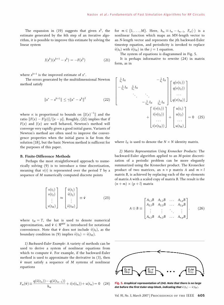
for m 2 f1; . . . ;Mg. Here, hm * tm % tm%1, Fm!&" is anonlinear function which maps an MN-length vector toan N-length vector and represents the jth backward-Eulertimestep equation, and periodicity is invoked to replacev!t0" with v!tM" in the j $ 1 equation.

The system of equations is diagrammed in Fig. 5.It is perhaps informative to rewrite (24) in matrix

form, as in

1h1IN % 1

h1IN

% 1h2IN 1

h2IN

. .. . .

.

% 1hMIN 1

hMIN

2

6

6

6

6

6

6

4

3

7

7

7

7

7

7

5

q v!t1"! "q v!t2"! ". . .

q v!tM"! "

2

6

6

6

4

3

7

7

7

5

#

i v!t1"! "i v!t2"! ". . .

i v!tM"! "

2

6

6

6

4

3

7

7

7

5

#

u!t1"u!t2". . .

u!tM"

2

6

6

6

4

3

7

7

7

5

$ 0 (25)

where IN is used to denote the N ' N identity matrix.

2) Matrix Representation Using Kronecker Products: Thebackward-Euler algorithm applied to an M-point discreti-zation of a periodic problem can be more elegantlysummarized using the Kronecker product. The Kroneckerproduct of two matrices, an n' p matrix A and m' lmatrix B, is achieved by replacing each of the np elementsof matrix A with a scaled copy of matrix B. The result is the!n# m" ' !p# l" matrix

A. B *

A1;1B A1;2B . . . A1;pBA2;1B A2;2B . . . A2;pB

..

. ... . .

. ...

An;1B An;2B . . . An;pB

2

6

6

6

4

3

7

7

7

5

: (26)

Fig. 5. Graphical representation of (24). Note that there is no large

dot before the first Euler-step block, indicating that v!t0" $ v!tM".



The Kronecker product notation makes it possible tosummarize the backward-Euler M-step periodic discretiza-tion with an M'M differentiation matrix

Dbe $

1h1

% 1h1

% 1h2

1h2

. .. . .

.

% 1hM

1hM;

2

6

6

6

6

4

3

7

7

7

7

5

(27)

and then apply the backward-Euler periodic discretizationto an N-dimensional differential equation system using theKronecker product. For example, (25) becomes

F!v" $ Dbe . INq!v" # i!v" # u $ 0 (28)

where IN is the N ' N identity matrix and

q!v"*

q v!t1"! "q v!t2"! "

..

.

q v!tm"! "

2

6

6

6

6

4

3

7

7

7

7

5

; i!v"*

i v!t1"! "i v!t2"! "

..

.

i v!tm"! "

2

6

6

6

6

4

3

7

7

7

7

5

;

u*

u!t1"u!t2"

..

.

u!tM""

2

6

6

6

6

4

3

7

7

7

7

5

: (29)

One elegant aspect of the matrix form in (28) is theease with which it is possible to substitute more accuratebackward or forward discretization methods to replacebackward-Euler. It is only necessary to replace Dbe in (28).For example, the L-step backward difference methods [32]estimate a time derivative using several backward time-points, as in

d

dtq v!tm"! " ,

X

L

j$0

$mj q v!tm%j"& '

: (30)

Note that for backward-Euler, L $ 1 and

$m0 $ $m

1 $ 1

hm(31)

and note also that $mj will be independent of m if all the

timesteps are equal. To substitute a two-step backward-

difference formula in (28), Dbe is replaced by Dbd2

where

Dbd2 $

$10 0 . . . 0 $1

2 $11

$21 $2

0 0 . . . 0 $22

$32 $3

1 $30 0 . . . 0

. .. . .

. . ..

0 . . . 0 $M2 $M

1 $M0

2

6

6

6

6

6

6

4

3

7

7

7

7

7

7

5

: (32)

3) Trapezoidal Rule RC Example: The Trapezoidal rule isnot a backward or forward difference formula but can stillbe used to compute steady-state solutions using a minormodification of the above finite-difference method. TheTrapezoidal method is also interesting to study in thissetting because of a curious property we will make clear byexample.

Again consider the differential equation for the RCcircuit from (12), repeated here reorganized and with greplacing 1=r

cd

dtv!t" $ %gv!t" % u!t": (33)

The mth timestep of the Trapezoidal rule applied tocomputing the solution to (33) is

c

hmv!tm" % v!tm%1"! "

$ % 1

2gv!tm" # u!tm" # gv!tm%1" # u!tm%1"! " (34)

and when used to compute a periodic steady-state solutionyields the matrix equation

ch1# 0:5g 0 . . . 0 % c

h1# 0:5g

% ch2# 0:5g c

h2# 0:5g 0 . . . 0

. ..

0 . . . 0 % chM# 0:5g c

hM# 0:5g

2

6

6

6

6

6

4

3

7

7

7

7

7

5

'

v!t1"v!t2"

..

.

v!tM"

2

6

6

6

6

4

3

7

7

7

7

5

$

0:5 u!t1" # u!tM"! "0:5 u!t2" # u!t1"! "

..

.

0:5 #u!tM" # u!tM%1"! "

2

6

6

6

6

4

3

7

7

7

7

5

: (35)

Now suppose the capacitance approaches zero, then thematrix in (35) takes on a curious property. If the number of



timesteps M, is odd, then a reasonable solution iscomputed. However, if the number of timesteps is even,then the matrix in (35) is singular, and the eigenvectorassociated with the zero eigenvalue is of the form

1:0

%1:0

1:0

%1:0...

1:0

%1:0

2

6

6

6

6

6

6

6

6

6

6

6

4

3

7

7

7

7

7

7

7

7

7

7

7

5

: (36)

The seasoned circuit simulation user or developer mayrecognize this as the periodic steady-state representationof an artifact known as the trapezoidal rule ringing problem[33]. Nevertheless, the fact that the ringing appears anddisappears simply by incrementing the number of time-steps makes this issue the numerical equivalent of a prettygood card trick, no doubt useful for impressing one’s guestsat parties.

4) Jacobian for Newton’s Method: Before deriving theJacobian needed to apply Newton’s method to (28), it isuseful (or perhaps just very appealing to the authors) tonote the simplicity with which the Kronecker product canbe used to express the linear algebriac system which mustbe solved to compute the steady-state solution associatedwith the finite-difference method applied to the lineardifferential equation system in (4). For this case, (28)simplifies to

!Dfd . C # IM . G"v $ u (37)

where Dfd is the differentiation matrix associated with theselected finite-difference scheme.

The Jacobian for F!&" in (28) has structural similaritiesto (37) but will require the M derivative matricesCm $ dq!v!tm""=dv a n d Gm $ di!v!tm""=dv f o r m 2f1; . . . ;Mg. By first defining the MN 'MN block diagonalmatrices

C $

C1 0 0 . . . 00 C2 0 . . . 0

. ..

. ..

0 0 . . . 0 CM

2

6

6

6

6

6

4

3

7

7

7

7

7

5

(38)

and

G $

G1 0 0 . . . 00 G2 0 . . . 0

. ..

. ..

0 0 . . . 0 GM

2

6

6

6

6

6

4

3

7

7

7

7

7

5

(39)

it is possible to give a fairly compact form to represent theMN 'MN Jacobian of F!&" in (28)

JF!v" $ !Dfd . IN"C # G: (40)

C. Basis Collocation MethodsAn alternative to the finite-difference method for

solving (9) is to represent the solution approximately as aweighted sum of basis functions that satisfy the periodicityconstraint and then generate a system of equations forcomputing the weights. In circuit simulation, the mostcommonly used techniques for generating equations forthe basis function weights are the so-called spectralcollocation methods [44]. The name betrays a history ofusing sines and cosines as basis functions, though otherbases, such as polynomials and wavelets, have found recentuse [41], [45]. In spectral collocation methods, the solutionis represented by the weighted sum of basis functions thatexactly satisfy the differential equation, but only at a set ofcollocation timepoints.

The equations for spectral collocation are most easilyderived if the set of basis functions have certainproperties. To demonstrate those properties, consider abasis set being used to approximate a periodic functionx!t", as in

x!t" ,X

K

k$1

X(k)%k!t" (41)

where %k!t" and X(k), k 2 1; . . . ;K are the periodic basisfunctions and the basis function weights, respectively. Wewill assume that each of the %k!t"’s in (41) aredifferentiable, and in addition we will assume the basisset must have an interpolation property. That is, it must bepossible to determine uniquely the K basis functionweights given a set of K sample values of x!t", thoughthe sample timepoints may depend on the basis. This



interpolation condition implies that there exists a set of Ktimepoints, t1; . . . tK , such that the K ' K matrix

"%1 *%1!t1" . . . %K!t1"

..

. ...

%1!tK" . . . %K!tK"

2

6

4

3

7

5(42)

is nonsingular and therefore the basis function coefficientscan be uniquely determined from the sample points using

X1

..

.

XK

2

6

4

3

7

5$ "

x!t1"...

x!tK"

2

6

4

3

7

5: (43)

To use basis functions to solve (9), consider expandingq!v!t"" in (9) as

q v!t"! " ,X

K

k$1

Q(k)%k!t" (44)

where Q(k) is the N-length vector of weights for the kthbasis function.

Substituting (44) in (3) yields

d

dt

X

K

k$1

Q(k)%k!t"

!

# i v!t"! " # u!t" , 0: (45)

Moving the time derivative inside the finite sum simplifies(45) and we have

X

K

k$1

Q(k) _%k!t" # i v!t"! " # u!t" , 0 (46)

where note that the dot above the basis function is used todenote the basis function time derivative.

In order to generate a system of equations for theweights, (46) is precisely enforced at M collocation pointsft1; . . . ; tMg,

X

K

k$1

Q(k) _%k!tm" # i v!tm"! " # u!tm" $ 0 (47)

for m 2 f1; . . . ;Mg. It is also possible to generateequations for the basis function weights by enforcing

(46) to be orthogonal to each of the basis functions. Suchmethods are referred to as Galerkin methods [7], [44], [46]and have played an important role in the development ofperiodic steady-state methods for circuits though they arenot the focus in this paper.

If the number of collocation points and the number ofbasis functions are equal, M $ K, and the basis set satisfiesthe interpolation condition mentioned above with anM'M interpolation matrix ", then (47) can be recastusing the Kronecker notation and paralleling (28) as

F!v" $ _"%1". INq!v" # i!v" # u $ 0 (48)

where IN is the N ' N identity matrix and

_"%1 *_%1!t1" . . . _%K!t1"... ..

.

_%1!tK" . . . _%K!tK"

2

6

4

3

7

5: (49)

By analogy to (28), the product _"%1" in (48) can bedenoted as a basis function associated differentiationmatrix Dbda

Dbda $ _"%1" (50)

and (48) becomes identical in form to (28)

F!v" $ Dbda . INq!v" # i!v" # u $ 0: (51)

Therefore, regardless of the choice of the set of basisfunctions, using the collocation technique to compute thebasis function weights implies the resulting method isprecisely analgous to a finite-difference method with aparticular choice of discretization matrix. For the backward-difference methods described above, the M'M matrix Dfd

had only orderM nonzeros, but as we will see in the Fourierexample that follows that for spectral collocation methodsthe Dbda matrix is typically dense.

Since basis collocation methods generate nonlinearsystems of equations that are structurally identical to thosegenerated by the finite-difference methods, when New-ton’s is used to solve (51), the formula for the requiredMN 'MN Jacobian of F!&" in (51) follows from (40) and isgiven by

JF !v"! " $ !Dbda . IN"C # G (52)

where C and G are as defined in (38) and (39).



1) Fourier Basis Example: If a sinusoid is the input to asystem of differential equations generated by a linear time-invariant circuit, then the associated periodic steady-statesolution will be a scaled and phase-shifted sinusoid of thesame frequency. For a mildly nonlinear circuit with asinusoidal input, the solution is often accurately repre-sented by a sinusoid and a few of its harmonics. Thisobservation suggests that a truncated Fourier series will bean efficient basis set for solving periodic steady-stateproblems of mildly nonlinear circuits.

To begin, any square integrable T-periodic waveformx!t" can be represented as a Fourier series

x!t" $X

k$1

k$%1X(k)ej2&fkt (53)

where fk $ kt=T and

X(k) $ 1

T

Z

T=2

%T=2

x!t"e%j2&fktdt: (54)

If x!t" is both periodic and is sufficiently smooth, (e.g.,infinitely continuously differentiable), then X(k) ! 0exponentially fast with increasing k. This implies x!t"can be accurately represented with a truncated Fourierseries, that is x!t" , x!t" where x!t" is given by thetruncated Fourier series

x!t" $X

k$K

k$%K

X(k)ej2&fkt (55)

where the number of harmonics K is typically fewer thanone hundred. Note that the time derivative of x!t" isgiven by

d

dtx!t" $

X

k$K

k$%K

X(k)j2&fkej2&fkt: (56)

If a truncated Fourier series is used as the basis set whenapproximately solving (9), the method is referred to asharmonic balance [6] or a Fourier spectral method [17].

If theM $ 2K # 1 collocation timepoints are uniformlydistributed throughout a period from %!T=2" to T=2, as intm $ !!m% !K # 1=2""=M"!1=T", then the associated in-terpolation matrix "F is just the discrete Fourier transformand "%1

F is the inverse discrete Fourier transform, each ofwhich can be applied in orderM logM operations using the

fast Fourier transform and its inverse. In addition, _"%1F ,

representing the time derivative of the series representa-tion, is given by

_"%1F $ "%1

F # (57)

where # is the diagonal matrix given by

# *

j2&fKj2&fK%1

. .. . .

.

j2&f%K

2

6

6

6

4

3

7

7

7

5

: (58)

The Fourier basis collocation method generates asystem of equations of the form (51), where

DF $ "%1#" (59)

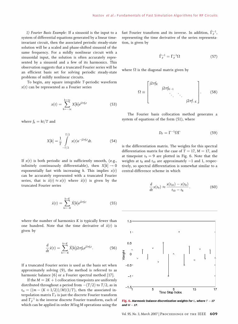
is the differentiation matrix. The weights for this spectraldifferentiation matrix for the case of T $ 17, M $ 17, andat timepoint t9 $ 9 are plotted in Fig. 6. Note that theweights at t8 and t10 are approximately %1 and 1, respec-tively, so spectral differentiation is somewhat similar to acentral-difference scheme in which

d

dtx!t9" ,

x!t10" % x!t8"t10 % t8

: (60)

Fig. 6. Harmonic balance discretization weights for t9 where T $ 17

andM $ 17.



The connection between spectral differentiation andstandard differencing schemes can be exploited whendeveloping fast methods for computing solutions to (28)and (51), a point we will return to subsequently.

The error analysis of spectral-collocation methods canbe found in [17] and [19]. Also, many implementations ofharmonic balance in circuit simulators use spectralGalerkin methods rather than collocation schemes [7],and if a small number of harmonics are used, Galerkinspectral methods can have superior accuracy and oftenlead to nonlinear systems of equations that are more easilysolved with Newton’s method [47].

D. Shooting MethodsThe numerical procedure for solving the state transi-

tion function based periodic steady-state formulation in(11) is most easily derived for a specific discretizationscheme and then generalized. Once again, considerapplying the simple backward-Euler algorithm to (3).Given any v!t0", the nonlinear equation

q v!t1"! " % q v!t0"! "h1

# i v!t1"! " # u!t1" $ 0 (61)

can be solved, presumably using a multidimensionalNewton method, for v!t1". Then, v!t1" can be used to solve

q v!t2"! " % q v!t1"! "h2

# i v!t2"! " # u!t2" $ 0 (62)

for v!t2". This procedure can be continued, effectivelyintegrating the differential equation one timestep at a timeuntil v!tm" has been computed. And since the nonlinearequations are solved at each timestep, v!tm" is an implicitlydefined algebraic function of v!t0". This implicitly definedfunction is a numerical approximation to the state-transition function !!&" described in the previous section.That is,

v!tm" $ ! v!t0"; tm! " , ! v!t0"; tm! ": (63)

The discretized version of the state-transition function-based periodic steady-state formulation is then

F v!tm"! " * v!tM" % ! v!tM"; tM! " $ 0: (64)

Using (64) to compute a steady-state solution is oftenreferred to as a shooting method, in which one guesses aperiodic steady state and then shoots forward one periodwith the hope of arriving close to the guessed initial state.

Then, the difference between the initial and final states isused to correct the initial state, and the method shootsforward another period. As is commonly noted in thenumerical analysis literature, this shooting procedure willbe disasteriously ineffective if the first guess at a periodicsteady state excites rapidly growing unstable behavior inthe nonlinear system [18], but this is rarely an issue forcircuit simulation. Circuits with such unstable Bmodes[are unlikely to be useful in practice, and most circuitdesigners using periodic steady-state analysis have alreadyverified that their designs are quite stable.

The state correction needed for the shooting methodcan be performed with Newton’s method applied to (64),in which case the correction equation becomes

IN % J! vk!tM"; T& '( )

vk#1!tM" % vk!tM"( )

$ %Fsh vk!tM"& '

(65)

where k is the Newton iteration index, IN is N ' N identitymatrix, and

J!!v; T" *d

dv!!v; T" (66)

is referred to as discretized sensitivity matrix.To complete the description of the shooting-Newton

method, it is necessary to present the procedure for com-puting !!v; T" and J!!v; T". As mentioned above, computingthe approximate state transition function is equivalent tosolving the backward-Euler equations as in (24) one time-step at a time. Solving the backward-Euler equations isusually accomplished using an inner Newton iteration, as in

Cmklhm

# Gmkl

$ %

vk;!l#1"!tm" % vk;l!tm"* +

$ % 1

hm

' q vk;l!tm"& '

% q vk;l!tm"& '& '

% i vk;l!tm"& '

% u!tm" (67)

where m is the timestep index, k is the shooting-Newtoniteration index, l is the inner Newton iteration index,Cmkl $ !dq!vk;l!tm""=dv and Gmkl $ !di!vk;l!tm""=dv. Some-times, there are just too many indices.

To see how to compute J!!v; T" as a by-product of theNewton method in (67), let l $ + denote the inner Newtoniteration index which achieves sufficent convergence andlet vk;+!tm" denote the associated inner Newton convergedsolution. Using this notation

q vk;+!tm"! "% q vk;+!tm%1"! "hm

# i vk;+!tm"& '

# u!tm"$ 'm (68)



where the left-hand side of (68) is almost zero, so that 'm isbounded by the inner Newton convergence tolerance.

Implicitly differentiating (68) with respect to v, andassuming that 'm is independent of v, results in

Cmk+hm

# Gmk+

$ %

dvk;+!tm"dv

$C!m%1"k+

hm

dvk;+!tm%1"dv

(69)

where it is usually the case that the matrices Cmk+=hm andGmk+ are available as a by-product of the inner Newtoniteration.

Recursively applying (69), with the initial valuevk;+!t0" $ v, yields a product form for the Jacobian

J!!v; tM" $Y

M

m$1

Cmk+hm

# Gmk+

$ %%1C!m%1"k+

hm(70)

where the notationQM

m$1 indicates the M-term productrather than a sum [15].

1) Linear Example: If a fixed timestep backward-Eulerdiscretization scheme is applied to (4), then

C

hv!tm" % v!tm%1"! " # Gv!tm" # u!tm" $ 0 (71)

for m 2 f1; . . . ;Mg, where periodicity implies thatv!tM" $ v!t0". Solving for v!tM" yields a linear systemof equations

(IN % J!)v!tM" $ b (72)

where J! is the derivative of the state transition function,or the sensitivity matrix, and is given by

J! $ C

h# G

" #%1C

h

" #M

(73)

and the right-hand side N-length vector b is given by

b $X

M

m$1

C

h# G

" #%1C

h

" #mC

h# G

" #%1

u!tM%m": (74)

It is interesting to compare (72) and (74) to (16), note howthe fixed-timestep backward-Euler algorithm is approxi-

mating the matrix exponential in (73) and the convolutionintegral in (74).

2) Comparing to Finite-Difference Methods: If Newton’smethod is used for both the shooting method, as in (65),and for the finite difference method, in which case theJacobian is (40), there appears to be an advantage for theshooting-Newton method. The shooting-Newton methodis being used to solve a system of N nonlinear equations,whereas the finite-difference-Newton method is beingused to solve an NM system of nonlinear equations. Thisadvantage is not as significant as it seems, primarilybecause computing the sensitivity matrix according to (70)is more expensive than computing the finite-differenceJacobian. In this section, we examine the backward-Eulerdiscretized equations to show that solving a system theshooting method Jacobian, as in (65), is nearly equivalentto solving a preconditioned system involving the finite-difference method Jacobian, in (40).

To start, let L be the NM' NM the block lowerbidiagonal matrix given by

L *

C1h1# G1

% C1h2

C2h2# G2

. .. . .

.

% CM%1

hMCMhM

# GM

2

6

6

6

6

4

3

7

7

7

7

5

(75)

and define B as the NM' NM matrix with a singlenonzero block

B *

0 . . . 0 CMh1

0. .. . .

.

0 0

2

6

6

4

3

7

7

5

(76)

where Cm and Gm are the N ' N matrices which denotedq!v!tj""=dv and di!v!tj""=dv, respectively.

The matrix L defined in (75) is block lower bidiagonal,where the diagonal blocks have the same structure as thesingle timestep Jacobian in (67). It then follows that thecost of applying L%1 is no more than computing oneNewton iteration at each of M timesteps. One simplyfactors the diagonal blocks of L and backsolves. Formally,the result can be written as

!INM % L%1B"!~vk#1 % ~vk" $ %L%1F!~vk" (77)

though L%1 would never be explicitly computed. Here, INMis the NM' NM identity matrix.



Examining (77) reveals an important feature, that L%1Bis an NM' NM matrix whose only nonzero entries are inthe last N columns. Specifically,

!INM % L%1B" $

IN 0 0 . . . 0 %P10 IN 0 . . . 0 %P2... . .

. . .. . .

. ... ..

.

..

. . .. . .

. . ..

0 %PM%2

..

. . .. . .

. . ..

IN %PM%1

0 . . . . . . . . . 0 IN % PM

2

6

6

6

6

6

6

6

6

4

3

7

7

7

7

7

7

7

7

5

(78)

where the N ' N matrix PM is the N!M% 1" # 1 throughNM rows of the lastN columns of L%1B. This bordered-blockdiagonal form implies that ~vk#1 % ~vk in (77) can be com-puted in three steps. The first step is to compute PM, thesecond step is to use the computed PM to determine the lastN entries in ~vk#1 % ~vk. The last step in solving (77) is tocompute the rest of ~vk#1 % ~vk by backsolving with L.

The close relation between solving (77) and (65) cannow be easily established. If L and B are formed using Cmk+and Gmk+ as defined in (69), then by explicitly computingL%1B it can be shown that the shooting method JacobianJ!!vk!t0"; tM" is equal to PM. The importance of thisobservation is that solving the shooting-Newton updateequation is nearly computationally equivalent to solving apreconditioned finite-difference-Newton update (77). Thecomparison can be made precise if q!v" and i!v" are linear,so that the C and Gmatrices are independent of v, then thevk#1!tM" % vk!tM" produced by the kth iteration of New-ton’s method applied to the finite-difference formulationwill be identical to the vk#1!tM" % vk!tM" produced bysolving (65).

An alternative interpretation of the connection be-tween shooting-Newton and finite-difference-Newtonmethods is to view the shooting-Newton method as atwo-level Newton method [10] for solving (24). In theshooting-Newton method, if v!tm" is computed by using aninner Newton method to solve the nonlinear equation Fmat each timestep, starting with v!to" $ v!tM", or equiva-lently if v!tm" is computed by evaluating !!v!tM"; tm", thenFi!v" in (24) will be nearly zero for i 2 f1; . . . ;M% 1g,regardless of the choice of v!tM". Of course, !!v!tM"; tM"will not necessarily be equal to v!tM"; therefore, FM!v" willnot be zero, unless v!tM" $ v!t0" is the right initialcondition to produce the periodic steady state. In theshooting-Newton method, an outer Newton method is usedto correct v!tM". The difference between the two methodscan then be characterized by differences in inputs to thelinearized systems, as diagrammed in Fig. 7.

3) More General Shooting Methods: Many finite-difference methods can be converted to shooting methods,but only if the underlying time discretization schemetreats the periodicity constraint by Bwrappping around[ asingle final timepoint. For discretization schemes whichsatisfy this constraint, the M'M periodic differentiationmatrix, D, is lower triangular except for a single entry inthe upper right-hand corner. As an example, the differ-entiation matrix Dbe in (27) is lower bidiagonal exceptfor a single entry in the upper right-hand corner. To bemore precise, if

Di;j $ 0; j 9 i; i 6$ 1; j 6$ M (79)

consider separating D into its lower triangular part, DL,and a single entry D1;M. The shooting method can then

Fig. 7. Diagram of solving backward-Euler discretized finite-difference-Newton iteration equation (top picture) and solving shooting-Newton

iteration equation (bottom picture). Note that for shooting method the RHS contribution at intermediate timesteps is zero, due to the inner

newton iteration.



be compactly described as solving the nonlinear al-gebriac system

F!vT" $ vT % ~e TM . IN& '

v $ 0 (80)

for the N-length vector vT , where~eM an M-length vector ofzeros except for unity in the Mth entry as in

~eM $

0...

01

2

6

6

4

3

7

7

5

(81)

and v is anMN-length vector which is an implicitly definedfunction of vT . Specifically, v is defined as the solution tothe system of MN nonlinear equations

DL . INq!v" # i!v" # u# !D1;M~e1" . q!vT" $ 0 (82)

where ~e1 is the M-length vector of zeros except for unityin the first entry. Perhaps the last Kronecker termgenerating an NM-length vector in (82) suggests that theauthors have become carried away and overused theKronecker product, as

!D1;M~e1" . q!vT" $

D1;Mq!vT"0...

0

2

6

6

4

3

7

7

5

(83)

is more easily understood without the use of the Kroneckerproduct, but the form will lend some insight, as will beclear when examining the equation for the Jacobian.

If Newton’s method is used to solve (80), then note aninner Newton’s method will be required to solve (82). TheJacobian associated with (80) can be determined usingimplicit differentiation and is given by

Jshoot!vT" $ IN # ~e TM . IN& '

!DL . IN"C # G& '%1

' D1;M~e1 .@q!vT"@v

" #

(84)

where C and G are as defined in (38) and (39), and!!DL . IN"C # G is a block lower triangular matrix whoseinverse is inexpensive to apply.

IV. FAST METHODS

As described in the previous section, the finite-differencebasis-collocation and shooting methods all generatesystems of nonlinear equations that are typically solvedwith the multidimensional Newton’s method. The stan-dard approach for solving the linear systems that generatethe Newton method updates, as in (21), is to use sparsematrix techniques to form and factor an explicit represen-tation of the Newton method Jacobian [6], [12]. When thisstandard approach is applied to computing the updates forNewton’s method applied to any of the periodic steady-state methods, the cost of forming and factoring theexplicit Jacobian grows too fast with problem size and themethod becomes infeasible for large circuits.

It is important to take note that we explicitly mentionthe cost of forming the explicit Jacobian. The reason is thatfor all the steady-state methods described in the previoussection, the Jacobians were given in an implicit form, as acombination of sums, products, and possibly Kroneckerproducts. For the backward-Euler based shooting method,the N ' N Jacobian Jshoot, is

Jshoot $ IN %Y

M

m$1

Cmhm

# Gm

$ %%1Cmhm

" #

(85)

and is the difference between the identity matrix and aproduct of M N ' N matrices, each of which must becomputed as the product of a scaled capacitance matrixand the inverse of a weighted sum of a capacitance and aconductance matrix. The NM' NM finite-difference orbasis-collocation Jacobians, denoted generally as Jfdbc, arealso implicitly defined. In particular

Jfdbc $ !D. IN"C # G (86)

is constructed from an M'M differentiation matrix D, aset of M N ' N capacitance and conductance matriceswhich make up the diagonal blocks of C and G, and anN ' N identity matrix.

Computing the explicit representation of the Jacobianfrom either (85) or (86) is expensive, and therefore anyfast method for these problems must avoid explicitJacobian construction. Some specialized methods withthis property have been developed for shooting methodsbased on sampling results of multiperiod transientintegration [25], and specialized methods have beendeveloped for Fourier basis collocation methods whichuse Jacobian approximations [36]. Most of these methodshave been abandoned in favor of solving the Newtoniteration equation using a Krylov subspace method, such asthe generalized minimum residual method (GMRES) andthe quasi-minimum residual method (QMR) [9], [27].



When combined with good preconditioners, to be discussedsubsequently, Krylov subspace methods reliably solvelinear systems of equations but do not require an explicitsystem matrix. Instead, Krylov subspace methods onlyrequire matrix-vector products, and such products can becomputed efficiently using the implicit forms of theJacobians given above.

Claiming that Krylov subspace methods do not requireexplicit system matrices is somewhat misleading, as thesemethods converge quite slowly without a good precondi-tioner, and preconditioners often require that at least someof the system matrix be explicitly represented. In thefollowing section, we describe one of the Krylov subspacemethods, GMRES, and the idea of preconditioning. In thesubsections that follow we address the issue of precondi-tioning, first demonstrating why Krylov subspace methodsconverge rapidly for shooting methods even withoutpreconditioning, then describing lower triangular andaveraging based preconditioning for basis-collocation andfinite-difference methods, drawing connections to shoot-ing methods when informative.

A. Krylov Subspace MethodsKrylov subspace methods are the most commonly used

iterative technique for solving Newton iteration equationsfor periodic steady-state solvers. The two main reasons forthe popularity of this class of iterative methods are thatonly matrix-vector products are required, avoiding explic-itly forming the system matrix, and that convergence israpid when preconditioned effectively.

As an example of a Krylov subspace method, considerthe generalized minimum residual algorithm, GMRES [9].A simplified version of GMRES applied to solving a genericproblem is given as follows.

GMRES Algorithm for Solving Ax $ bGuess at a solution, x0.Initialize the search direction p0 $ b% Ax0.Set k $ 1.do {Compute the new search direction, pk $ Apk%1.Orthogonalize, pk $ pk %

Pk%1j$0 (k;jpj.

Choose $k in xk $ xk%1 # $kpk

to minimize krkk $ kb% Axkk.If krkk G tolerancegmres, return vk as the solution.else Set k $ k# 1.

}

Krylov subspace methods converge rapidly when appliedto matrices which are not too nonnormal and whoseeigenvalues are contained in a small number of tight clusters[44]. Therefore, Krylov subspace methods converge rapidlywhen applied to matrices which are small perturbations fromthe identity matrix, but can, as an example, convergeremarkably slowly when applied to a diagonal matrix whosediagonal entries are widely dispersed. In many cases,

convergence can be accelerated by replacing the originalproblem with a preconditioned problem

PAX $ Pb (87)

where A and b are the original system’s matrix and right-hand side, and P is the preconditioner. Obviously, thepreconditioner that best accelerates the Krylov subspacemethod is P $ A%1, but were such a preconditioner avail-able, no iterative method would be needed.

B. Fast Shooting MethodsApplying GMRES to solving the backward-Euler

discretized shooting Newton iteration equation is straight-forward, as multiplying by the shooting method Jacobian in(85) can be accomplished using the simple M-stepalgorithm as follows.

Computing pk $ Jshootpk%1

Initialize ptemp $ pk%1

For k $ 1 to M {Solve !!Cm=hm" # Gm"pk $ !Cm=hm"ptemp

Set ptemp $ pk

}Finalize pk $ pk%1 % pk

The N ' N Cm and Gm matrices are typically quitesparse, so each of the M matrix solutions required in theabove algorithm require roughly order N operations, whereorder!&" is used informally here to imply proportionalgrowth. Given the order N cost of the matrix solution inthis case, computing the entire matrix-vector productrequires order MN operations.

Note that the above algorithm can also be used N timesto compute an explicit representation of Jshoot, generatingthe explicit matrix one column at a time. To compute theith column, set pk%1 $~ei, where~ei can be thought of as theith unit vector or the ith column of the N ' N identitymatrix. Using this method, the cost of computing anexplicit representation of the shooting method Jacobianrequires order MN2 operations, which roughly equals thecost of performing N GMRES iterations.

When applied to solving the shooting-Newton iterationequation, GMRES and other Krylov subspace methodsconverge surprisingly rapidly without preconditioning andtypically require many fewer than N iterations to achievesufficient accuracy. This observation, combined with theabove analysis, implies that using a matrix-implicitGMRES algorithm to compute the shooting-Newton up-date will be far faster than computing the explicit shooting-Newton Jacobian.

In order to develop some insight as to why GMRESconverges so rapidly when applied to matrices like theshooting method Jacobian in (85), we consider the



linear problem (4) and assume the C matrix is invertibleso that A $ C%1G is defined as in (15). For this linearcase and a steady-state period T, the shooting methodJacobian is approximately

Jshoot , I% e%AT: (88)

Since eigenvalues are continuous functions of matrixelements, any eigenproperties of I% e%AT will roughlyhold for Jshoot, provided the discretization is accurate. Inparticular, using the properties of the matrix exponentialimplies

eig!Jshoot",eig!I% e%AT"$1%e%)iT i21; . . . n (89)

where )i is the ith eigenvalue of A, or in circuit terms, theinverse of the ith time constant. Therefore, if all but a fewof the circuit time constants are smaller than the steady-state period T, then e%)iT / 1 and the eigenvalues of Jshootwill be tightly clustered near one. That there might be afew Boutliers[ has a limited impact on Krylov subspacemethod convergence.

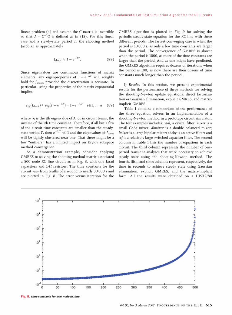
As a demonstration example, consider applyingGMRES to solving the shooting method matrix associateda 500 node RC line circuit as in Fig. 3, with one faradcapacitors and 1-# resistors. The time constants for thecircuit vary from tenths of a second to nearly 30 000 s andare plotted in Fig. 8. The error versus iteration for the

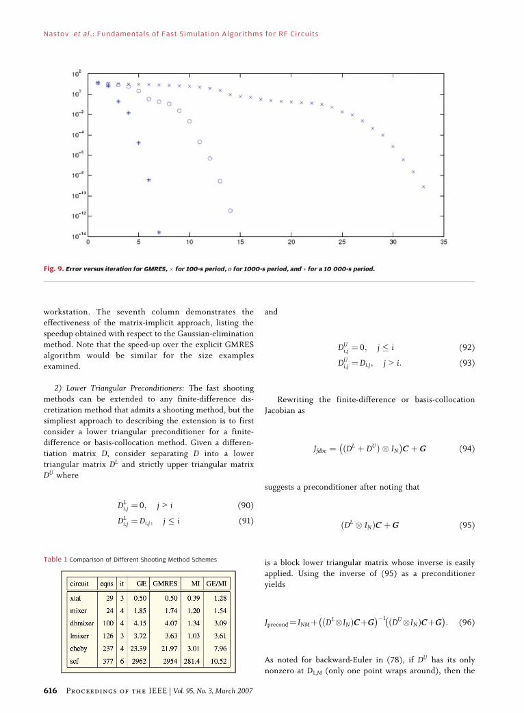
GMRES algorithm is plotted in Fig. 9 for solving theperiodic steady-state equation for the RC line with threedifferent periods. The fastest converging case is when theperiod is 10 000 s, as only a few time constants are largerthan the period. The convergence of GMRES is slowerwhen the period is 1000, as more of the time constants arelarger than the period. And as one might have predicted,the GMRES algorithm requires dozens of iterations whenthe period is 100, as now there are then dozens of timeconstants much longer than the period.

1) Results: In this section, we present experimentalresults for the performance of three methods for solvingthe shooting-Newton update equations: direct factoriza-tion or Gaussian elimination, explicit GMRES, and matrix-implicit GMRES.

Table 1 contains a comparison of the performance ofthe three equation solvers in an implementation of ashooting-Newton method in a prototype circuit simulator.The test examples includes: xtal, a crystal filter; mixer is asmall GaAs mixer; dbmixer is a double balanced mixer;lmixer is a large bipolar mixer; cheby is an active filter; andscf is a relatively large switched capacitor filter. The secondcolumn in Table 1 lists the number of equations in eachcircuit. The third column represents the number of one-period transient analyses that were necessary to achievesteady state using the shooting-Newton method. Thefourth, fifth, and sixth columns represent, respectively, thetime in seconds to achieve steady state using Gaussianelimination, explicit GMRES, and the matrix-implicitform. All the results were obtained on a HP712/80

Fig. 8. Time constants for 500 node RC line.



workstation. The seventh column demonstrates theeffectiveness of the matrix-implicit approach, listing thespeedup obtained with respect to the Gaussian-eliminationmethod. Note that the speed-up over the explicit GMRESalgorithm would be similar for the size examplesexamined.

2) Lower Triangular Preconditioners: The fast shootingmethods can be extended to any finite-difference dis-cretization method that admits a shooting method, but thesimpliest approach to describing the extension is to firstconsider a lower triangular preconditioner for a finite-difference or basis-collocation method. Given a differen-tiation matrix D, consider separating D into a lowertriangular matrix DL and strictly upper triangular matrixDU where

DLi;j $ 0; j 9 i (90)

DLi;j $Di;j; j - i (91)

and

DUi;j $ 0; j - i (92)

DUi;j $Di;j; j 9 i: (93)

Rewriting the finite-difference or basis-collocationJacobian as

Jfdbc $ !DL # DU" . IN& '

C # G (94)

suggests a preconditioner after noting that

!DL . IN"C # G (95)

is a block lower triangular matrix whose inverse is easilyapplied. Using the inverse of (95) as a preconditioneryields

Jprecond$ INM# !DL.IN"C#G& '%1 !DU.IN"C#G

& '

: (96)

As noted for backward-Euler in (78), if DU has its onlynonzero at D1;M (only one point wraps around), then the

Fig. 9. Error versus iteration for GMRES, ' for 100-s period, o for 1000-s period, and + for a 10 000-s period.

Table 1 Comparison of Different Shooting Method Schemes



preconditioned system will have a bordered blockdiagonal form

Jprecond $

IN 0 0 . . . 0 %P10 IN 0 . . . 0 %P2... . .

. . .. . .

. ... ..

.

..

. . .. . .

. . ..

0 %PM%2

..

. . .. . .

. . ..

IN %PM%1

0 . . . . . . . . . 0 IN % PM

2

6

6

6

6

6

6

6

6

4

3

7

7

7

7

7

7

7

7

5

(97)

where the N ' N matrix %PM is the N!M% 1" # 1 throughNM rows of the last N columns of

!DL . IN"C # G& '%1 !DU . IN"C # G

& '

: (98)

In particular, IN % PM will be precisely the generalshooting method matrix given in (84).

In the case when the differencing scheme admits ashooting method, the preconditioned system will usuallyhave its eigenvalues tightly clustered about one. To seethis, consider the structure of (97). Its upper blockdiagonal form implies that all of its eigenvalues are eitherone, due to the diagonal identity matrix blocks, or theeigenvalues of the shooting method matrix, which havealready been shown to cluster near one.

3) Averaging Preconditioners: Before describing pre-conditioners for the general finite-difference or basis-collocation Jacobians in (40) or (52), we considerfinite-difference or basis-collocation applied to the linearproblem in (4). The periodic steady-state solution can becomputed by solving the MN 'MN linear system

!D. C # IM . G"v $ u (99)

where D is the differentiation matrix for the selectedmethod. Explicitly forming and factoring !D. C # IM . G"can be quite computationally expensive, even though C andG are typically extremely sparse. The problem is that thedifferentation matrix D can be dense and the matrix will fillin substantially during sparse factorization.

A much faster algorithm for solving (99) whichavoids explicitly forming !D. C # IM . G" can be de-rived by making the modest assumption that D is diagon-alizable as in

D $ S)S%1 (100)

where ) is theM'M diagonal matrix of eigenvalues and Sis the M'M matrix of eigenvectors [41]. Using theeigendecompostion of D in (99) leads to

!S)S%1" . C # !SIMS%1" . G& '

v $ u: (101)

Using the Kronecker product property [29]

!AB" . !CD" $ !A. C"!B. D" (102)

and then factoring common expressions in (101) yields

!S. IN"!). C # IM . G"!S%1 . IN"& '

v $ u: (103)

Solving (103) for v

v $ !S%1 . IN"%1!). C # IM . G"%1!S. IN"%1& '

u:

(104)

The Kronecker product property that if A and B areinvertible square matrices

!A. B"%1 $ !A%1 . B%1" (105)

can be used to simplify (104)

v $ !S. IN"!). C # IM . G"%1!S%1 . IN"& '

u (106)

where !). C # IM . G"%1 is a block diagonal matrixgiven by

!)1C # G"%1 0 0 . . . 00 !)2C # G"%1 0 . . . 0

. ..

. ..

0 0 . . . 0 !)MC # G"%1

2

6

6

6

6

6

6

4

3

7

7

7

7

7

7

5

:

(107)

To compute v using (106) requires a sequence of threematrix-vector multiplications. Multiplying by !S%1 . IN"and !S. IN" each require NM2 operations. As (107) makesclear, multiplying by !). C # IM . G"%1 is M times thecost of applying !)1C # G"%1, or roughly order MN



operations as C and G are typically very sparse. Theresulting solution algorithm therefore requires

order!M3" # 2NM2 # order!MN" (108)

operations. The first term in (108) is the cost ofeigendecomposing D, the second term is the cost ofmultiplying by !S%1 . IN" and !S. IN", and third term isassociated with the cost of factoring and solving with thesparse matrices !)mC # G". The constant factors associatedwith the third term are large enough that it dominatesunless the number of timepoints, M, is quite large.

It should be noted that if D is associated with aperiodized fixed timestep multistep method, or with abasis-collocation method using Fourier series, then D willbe circulant. For circulant matrices, S and S%1 will beequivalent to the discrete Fourier transform matrix and itsinverse [28]. In these special cases, multiplication by S andS%1 can be performed in order MlogM operations using theforward and inverse fast Fourier transform, reducing thecomputational cost of (106) to

order!MlogM" # order!NMlogM" # order!MN" (109)

which is a substantial improvement only when thenumber of discretization timepoints or basis functions isquite large.

4) Extension to the Nonlinear Case: For finite-differenceand basis collocation methods applied to nonlinearproblems, the Jacobian has the form

Jfdbc!v" $ !D. IN"C # G (110)

where C and G are as defined in (38) and (39). In order toprecondition Jfdbc, consider computing averages of theindividual Cm and Gm matrices in the M diagonal blocks inC and G. Using these Cavg and Gavg matrices in (110) resultsin a decomposition

Jfdbc!v" $ !D. Cavg # IM . Gavg"# !D. IN"$C #$G! " (111)

where $C $ C % !IM . Cavg" and $G $ G% !IM . Gavg".To see how the terms involving Cavg and C in (111) werederived from (110), consider a few intermediate steps.First, note that by the definition of $C

!D. IN"C $ !D. IN" !IM . Cavg" #$C& '

(112)

which can be reorganized as

!D. IN"C $ !D. IN"!IM . Cavg" # !D. IN"$C: (113)

The first term on the right-hand side of (113) can besimplified using the reverse of the Kronecker property in(102). That is

!D. IN"!IM . Cavg" $ !DIM . INCavg" $ !D. Cavg" (114)

where the last equality follows trivially from the fact thatIM and IN are identity matrices. The result needed to derive(111) from (110) is then

!D. IN"C $ !D. Cavg" # !D. IN"$C: (115)

Though (111) is somewhat cumbersome to derive, itsform suggests preconditioning using !D. Cavg # IM.Gavg"%1, which, as shown above, is reasonbly inexpensiveto apply. The preconditioned Jacobian is then

!D. C # IM . G"%1Jfdbc!v" $ I#$DCG (116)

where

$DCG $ !D. C # IM . G"%1 !D. IN"$C #$G! ": (117)

If the circuit is only mildly nonlinear, then $DCG will besmall, and the preconditioned Jacobian in (117) will closeto the identity matrix and have tightly clustered eigenva-lues. As mentioned above, for such a case a Krylov-subspace method will converge rapidly.

5) Example Results: In this section, we present somelimited experimental results to both demonstrate thereduction in computation time that can be achieved usingmatrix-implicit iterative methods and to show the effec-tiveness of the averaging preconditioner.

In Table 2, we compare the megaflops required fordifferent methods to solve the linear system associatedwith a Fourier basis-collocation scheme. We compareGaussian elimination (GE), preconditioned explicitGMRES (GMRES), and matrix implicit GMRES (MI).Megaflops rather than CPU time are computed becauseour implementations are not uniformly optimized. Theexample used to generate the table is a distortion analysisof a 31-node CMOS operational transconductance ampli-fier. Note that for a 32 harmonic simulation, with 2232unknowns, the matrix-implicit GMRES is more than ten



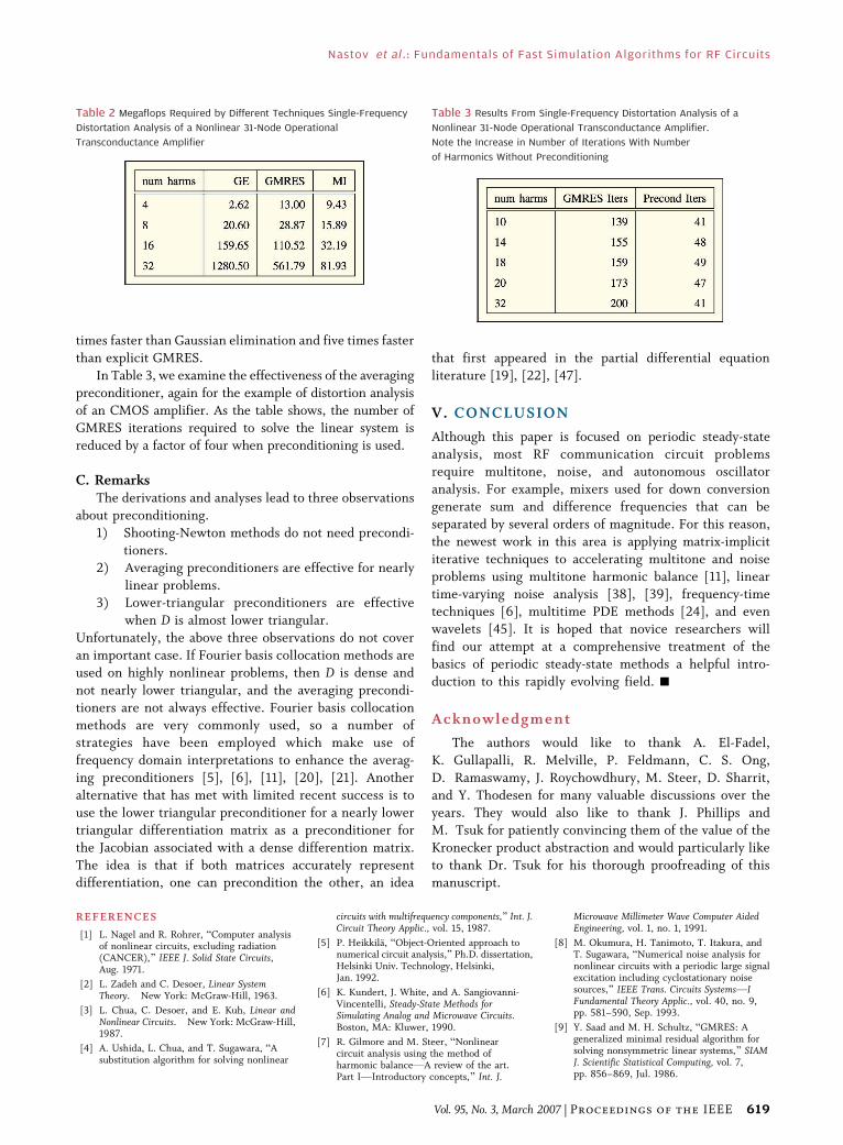
times faster than Gaussian elimination and five times fasterthan explicit GMRES.

In Table 3, we examine the effectiveness of the averagingpreconditioner, again for the example of distortion analysisof an CMOS amplifier. As the table shows, the number ofGMRES iterations required to solve the linear system isreduced by a factor of four when preconditioning is used.

C. RemarksThe derivations and analyses lead to three observations

about preconditioning.1) Shooting-Newton methods do not need precondi-

tioners.2) Averaging preconditioners are effective for nearly

linear problems.3) Lower-triangular preconditioners are effective

when D is almost lower triangular.Unfortunately, the above three observations do not coveran important case. If Fourier basis collocation methods areused on highly nonlinear problems, then D is dense andnot nearly lower triangular, and the averaging precondi-tioners are not always effective. Fourier basis collocationmethods are very commonly used, so a number ofstrategies have been employed which make use offrequency domain interpretations to enhance the averag-ing preconditioners [5], [6], [11], [20], [21]. Anotheralternative that has met with limited recent success is touse the lower triangular preconditioner for a nearly lowertriangular differentiation matrix as a preconditioner forthe Jacobian associated with a dense differention matrix.The idea is that if both matrices accurately representdifferentiation, one can precondition the other, an idea

that first appeared in the partial differential equationliterature [19], [22], [47].

V. CONCLUSION

Although this paper is focused on periodic steady-stateanalysis, most RF communication circuit problemsrequire multitone, noise, and autonomous oscillatoranalysis. For example, mixers used for down conversiongenerate sum and difference frequencies that can beseparated by several orders of magnitude. For this reason,the newest work in this area is applying matrix-implicititerative techniques to accelerating multitone and noiseproblems using multitone harmonic balance [11], lineartime-varying noise analysis [38], [39], frequency-timetechniques [6], multitime PDE methods [24], and evenwavelets [45]. It is hoped that novice researchers willfind our attempt at a comprehensive treatment of thebasics of periodic steady-state methods a helpful intro-duction to this rapidly evolving field. h

Acknowledgment

The authors would like to thank A. El-Fadel,K. Gullapalli, R. Melville, P. Feldmann, C. S. Ong,D. Ramaswamy, J. Roychowdhury, M. Steer, D. Sharrit,and Y. Thodesen for many valuable discussions over theyears. They would also like to thank J. Phillips andM. Tsuk for patiently convincing them of the value of theKronecker product abstraction and would particularly liketo thank Dr. Tsuk for his thorough proofreading of thismanuscript.

REFERENCES

[1] L. Nagel and R. Rohrer, BComputer analysisof nonlinear circuits, excluding radiation(CANCER),[ IEEE J. Solid State Circuits,Aug. 1971.

[2] L. Zadeh and C. Desoer, Linear SystemTheory. New York: McGraw-Hill, 1963.

[3] L. Chua, C. Desoer, and E. Kuh, Linear andNonlinear Circuits. New York: McGraw-Hill,1987.

[4] A. Ushida, L. Chua, and T. Sugawara, BAsubstitution algorithm for solving nonlinear

circuits with multifrequency components,[ Int. J.Circuit Theory Applic., vol. 15, 1987.

[5] P. Heikkila, BObject-Oriented approach tonumerical circuit analysis,[ Ph.D. dissertation,Helsinki Univ. Technology, Helsinki,Jan. 1992.

[6] K. Kundert, J. White, and A. Sangiovanni-Vincentelli, Steady-State Methods forSimulating Analog and Microwave Circuits.Boston, MA: Kluwer, 1990.

[7] R. Gilmore and M. Steer, BNonlinearcircuit analysis using the method ofharmonic balanceVA review of the art.Part IVIntroductory concepts,[ Int. J.

Microwave Millimeter Wave Computer AidedEngineering, vol. 1, no. 1, 1991.

[8] M. Okumura, H. Tanimoto, T. Itakura, andT. Sugawara, BNumerical noise analysis fornonlinear circuits with a periodic large signalexcitation including cyclostationary noisesources,[ IEEE Trans. Circuits SystemsVIFundamental Theory Applic., vol. 40, no. 9,pp. 581–590, Sep. 1993.

[9] Y. Saad and M. H. Schultz, BGMRES: Ageneralized minimal residual algorithm forsolving nonsymmetric linear systems,[ SIAMJ. Scientific Statistical Computing, vol. 7,pp. 856–869, Jul. 1986.

Table 2 Megaflops Required by Different Techniques Single-Frequency

Distortation Analysis of a Nonlinear 31-Node Operational

Transconductance Amplifier

Table 3 Results From Single-Frequency Distortation Analysis of a

Nonlinear 31-Node Operational Transconductance Amplifier.

Note the Increase in Number of Iterations With Number

of Harmonics Without Preconditioning



[10] N. Rabbat, A. Sangiovanni-Vincentelli, andH. Hsieh, BA multilevel Newton algorithmwith macromodeling and latency for theanalysis of large-scale non-linear circuits inthe time domain,[ IEEE Trans. Circuits Syst.,vol. 9, no. 1979, pp. 733–741.

[11] R.Melville, P. Feldmann, and J. Roychowdhury,BEfficient multi-tone distortion analysis ofanalog integrated circuits,[ in Proc. IEEECustom Integrated Circuits Conf., May 1995.

[12] L. T. Watson, Appl. Math. Comput., vol. 5,no. 1979, pp. 297–311.

[13] R. Telichevesky, K. S. Kundert, and J. K. White,BEfficient steady-state analysis based onmatrix-free Krylov-subspace methods,[ in Proc.Design Automation Conf., Santa Clara, CA,Jun. 1995.

[14] H. Keller, Numerical Solution of Two PointBoundary-Value Problems. Philadelphia, PA:SIAM, 1976.

[15] T. J. Aprille and T. N. Trick, BSteady-stateanalysis of nonlinear circuits with periodicinputs,[ Proc. IEEE, vol. 60, no. 1,pp. 108–114, Jan. 1972.

[16] J. P. Boyd, Chebyshev and Fourier SpectralMethods. New York: Springer-Verlag, 1989.

[17] D. Gottlieb and S. Orszag, Numerical Analysisof Spectral Methods: Theory and Applications.Philadelphia, PA: SIAM, 1977.

[18] J. Stoer and R. Burlisch, Introduction toNumerical Analysis. New York: Springer.

[19] C. Canuto, M. Y. Hussaini, A. Quarteroni, andT. A. Zang, Spectral Methods in FluidMechanics. New York: Springer-Verlag,1987.

[20] B. Troyanovsky, Z. Yu, L. So, and R. Dutton,BRelaxation-based harmonic balancetechnique for semiconductor devicesimulation,[ in Proc. Int. Conf. Computer-AidedDesign, Santa Clara, CA, Nov. 1995.

[21] M. M. Gourary, S. G. Rusakov, S. L. Ulyanov,M. M. Zharov, K. Gullapalli, andB. J. Mulvaney, BThe enhancing of efficiencyof the harmonic balance analysis by adaptationof preconditioner to circuit nonlinearity,[ inAsia and South Pacific Design Automation Conf.(ASP-DAC’00), p. 537.

[22] F. Veerse, BEfficient iterative timepreconditioners for harmonic balance RF

circuit simulation,[ in Proc. Int. Conf.Computer-Aided Design (ICCAD ’03), p. 251.

[23] H. G. Brachtendorf, G. Welsch, R. Laur, andA. Bunse-Gerstner, BNumerical steady stateanalysis of electronic circuits driven bymulti-tone signals,[ Electrical Eng., vol. 79,pp. 103–112, 1996.

[24] J. Roychowdhury, BAnalyzing circuits withwidely separated time scales using numericalPDE methods,[ IEEE Trans. Circuits Systems I:Fundamental Theory Applic., vol. 48, no. 5,pp. 578–594, 2001.

[25] S. Skelboe, BComputation of the periodicsteady-state response of nonlinear networksby extrapolation methods,[ IEEE Trans. Cts.Syst., vol. CAS-27, pp. 161–175, 1980.

[26] V. Rizzoli and A. Neri, BState of the art andpresent trends in nonlinear microwave CADtechniques,[ IEEE Trans. Microwave TheoryTech., vol. 36, no. 2, pp. 343–365, Feb. 1988.

[27] R. W. Freund, G. H. Golub, and N. M.Nachtigal, BIterative solution of linearsystems,[ Acta Numerica, pp. 57–100, 1991.

[28] C. V. Loan, Computational Frameworks for theFast Fourier Transform. Philadelphia, PA:SIAM, 1992.

[29] L. L. Whitcomb, Notes on Kronecker Products.[Online]. Available: spray.me.jhu.edu/llw/courses/me530647/kron_1.pdf.

[30] P. Feldmann, R. C. Melville, and D. Long,BEfficient frequency domain analysis of largenonlinear analog circuits,[ in Proc. IEEE CICC,May 1996.

[31] K. Kundert, J. White, and A. Sangiovanni-Vincentelli, BA mixed frequency-timeapproach for distortion analysis of switchingfilter circuits,[ IEEE J. Solid-State Cts., vol. 24,no. 2, pp. 443–451, Apr. 1989.

[32] C. W. Gear, Numerical Initial Value Problem inOrdinary Differential Equations. EnglewoodCliffs, NJ: Prentice-Hall, 1971.

[33] K. S. Kundert, The Designer’s Guide to SPICEand Spectre. Boston, MA: Kluwer, 1995.

[34] D. Feng, J. Phillips, K. Nabors, K. Kundert,and J. White, BEfficient computation of quasi-periodic circuit operating conditions via amixed frequency/time approach,[ in Proc.36th Design Automation Conf., Jun. 1999.

[35] J. Chen, D. Feng, J. Phillips, and K. Kundert,BSimulation and modeling of intermodulationdistortion in communication circuits,[ inProc. IEEE Custom Integrated Circuits Conf.,May 1999.

[36] K. Kundert, BIntroduction to RF simulationand its application,[ J. Solid-State Circuits,vol. 34, no. 9, Sep. 1999.

[37] Y. Thodeson and K. Kundert, BParametricharmonic balance,[ in Proc. IEEE MTT-S Int.Microwave Symp. Dig., Jun. 1996.

[38] R. Telichevesky, K. S. Kundert, andJ. K. White, BEfficient AC and noise analysisof two-tone RF circuits,[ in Proc. 33rd DesignAutomation Conf., Jun. 1996.

[39] J. Roychowdhury, D. Long, and P. Feldmann,BCyclostationary noise analysis of large RFcircuits with multi-tone excitations,[ IEEE J.Solid-State Circuits, Mar. 1998.

[40] R. Telichevesky, K. Kundert, I. El-Fadel, andJ. White, BFast simulation algorithms for RFcircuits,[ in Proc. IEEE Custom IntegratedCircuits Conf., May 1996.

[41] J. Phillips and B. Yang, BA multi-intervalChebyshev collocation method for efficienthigh-accuracy RF circuit simulation,[ inProc. 37th ACM/IEEE Design Automation Conf.(DAC 2000), Los Angeles, CA, Jun. 2000,pp. 178–183.

[42] K. Mayaram, D. C. Lee, S. Moinian, D. Rich,and J. Roychowdhury, BComputer-aidedcircuit analysis tools for RFIC simulation:Algorithms, features, and limitations,[ IEEETrans. CAS II, pp. 274–286, Apr. 2000.

[43] L. N. Trefethen, Spectral Methods in Matlab.Philadelphia, PA: SIAM, Jun. 2000.

[44] L. N. Trefethen and D. Bau, III, NumericalLinear Algebra. Philadelphia, PA: SIAM,1997.

[45] N. Soveiko and M. Nakhla, BWaveletharmonic balance,[ IEEE Microwave WirelessComponents Lett., Jul. 2003.

[46] O. J. Nastov and J. White, BTime-mappedharmonic balance,[ in Proc. IEEE DesignAutomation Conf., pp. 641–646.

[47] O. J. Nastov, BSpectral methods for circuitanalysis,[ Ph.D. dissertation, MassachusettsInst. Technol., Cambridge, 1999.

ABOUT THE AUTHORS

Rircardo Telichevesky (Member, IEEE) received

the B.S. degree in electrical engineering from the

Universidade Federal do Rio Grande do Sul, Brazil,

in 1985, the M.S. degree in electrical engineering

from the Technion, Israel, in 1988, and the Ph.D.

degree in electrical engineering and computer

science from the Massachusetts Institute of Tech-

nology, Cambridge, in 1994.

He specialized in computer architectures and

numerical simulation. He is the Principal Re-

searcher at Kineret Design Automation, Santa Clara, CA, working in the

simulation of analog and mixed signal systems. He played a key role in

the development of Cadence’s SpectreRF and Spectre simulator. He also

worked in the modeling and real-time simulation of physics-based

mechanical systems for virtual environments at Xulu Entertainment, Inc.

His current research interests include numerical algorithms and efficient

data structures for analog, RF, mixed signal, and system level simulation,

and its interoperability with other tools in the design flow.

Ken Kundert received the B.S. degree in 1979, the

M.S. degree in 1983, and the Ph.D. degree in

electrical engineering from the University of

California, Berkeley, in 1989.

He is renowned for creating two of the most

innovative, influential, and highest grossing circuit

simulators ever produced: Cadence’s Spectre and

Agilent’s harmonic balance simulator. He has a

deep understanding of analog/mixed-signal and

RF simulation technology and is well versed in its

application. He Co-founded Designer’s Guide Consulting, Inc., in 2005.

From 1989 to 2005, he worked at Cadence Design Systems as a Fellow. He

created Spectre and was the Principal Architect of the Spectre circuit

simulation family. As such, he has led the development of Spectre,

SpectreHDL, and SpectreRF. He also played a key role in the development

of Cadence’s AMS Designer and made substantial contributions to both

the Verilog-AMS and VHDL-AMS languages. Before that , he was a Circuit

Designer at Tektronix and Hewlett-Packard and contributed to the design

of the HP 8510 microwave network analyzer. He has written three books

on circuit simulation: The Designer’s Guide to Verilog-AMS in 2004, The

Designer’s Guide to SPICE and Spectre in 1995, and Steady-State Methods

for Simulating Analog and Microwave Circuits in 1990. He is the author of

11 patents.

Ognen Nastov, photograph and biography not available at the time of

publication.



Jacob White (Member, IEEE) received the B.S.

degree in electrical engineering and computer

science from the Massachusetts Institute of Tech-

nology, Cambridge, and the S.M. and Ph.D. degrees

in electrical engineering and computer science

from the University of California, Berkeley.

He worked at the IBM T.J. Watson Research

Center, from 1985 to 1987, and was the Analog

Devices Career Development Assistant Professor

at the Massachusetts Institute of Technology from

1987 to 1989. He is currently at the Massachusetts Institute of Technology

where he is the C. H. Green Professor in Electrical Engineering and

Computer Science. His research interests include numerical algorithms

for problems in the design and robust optimization of circuits,

interconnect, nanophotonics, carbon nanotubes, micromachining for

biological applications, biomolecules, and network models of biological

systems.

Dr. White was a 1988 Presidential Young Investigator and was an

Associate Editor of the IEEE TRANSACTIONS ON COMPUTER-AIDED DESIGN from

1992 until 1996. He was Chair of the International Conference on

Computer-Aided Design in 1999.



Documents

INVITED P A P E R Fundamentalsof … · P A P E R Fundamentalsof FastSimulationAlgorithms forRFCircuits The newest generationof circuit simulators perform periodic steady-state analysis