INVITED PAPER Collective Motion, Sensor …naomi/publications/2007/...INVITED PAPER Collective Motion, Sensor Networks, and Ocean Sampling The goal is design and control of optimum

INV ITEDP A P E R

Collective Motion, SensorNetworks, and Ocean SamplingThe goal is design and control of optimum trajectories for mobile sensor networks,

like a fleet of self-directed underwater gliders that move with ocean currents

and sample dynamic ocean variables.

By Naomi Ehrich Leonard, Fellow IEEE, Derek A. Paley, Student Member IEEE, Francois Lekien,

Rodolphe Sepulchre, Member IEEE, David M. Fratantoni, Member IEEE, and Russ E. Davis

ABSTRACT | This paper addresses the design of mobile sensor

networks for optimal data collection. The development is

strongly motivated by the application to adaptive ocean

sampling for an autonomous ocean observing and prediction

system. A performance metric, used to derive optimal paths for

the network of mobile sensors, defines the optimal data set as

one which minimizes error in a model estimate of the sampled

field. Feedback control laws are presented that stably coordi-

nate sensors on structured tracks that have been optimized

over a minimal set of parameters. Optimal, closed-loop solu-

tions are computed in a number of low-dimensional cases to

illustrate the methodology. Robustness of the performance to

the influence of a steady flow field on relatively slow-moving

mobile sensors is also explored.

KEYWORDS | Adaptive sampling; autonomous underwater

vehicles; cooperative control; coordinated dynamics; mobile

sensor networks; ocean sampling; underwater gliders

I . INTRODUCTION

The coupled physical and biological dynamics [1], [2] of

the oceans have a major impact on the environment, from

marine ecosystems to the global climate. In order to

understand, model, and predict these dynamics, oceano-graphers and ecologists seek measurements of tempera-

ture, salinity, flow, and biological variables across a range

of spatial and temporal scales [3]–[5]. Small spatial and

temporal scales drive the need for a mobile sensor network

rather than a static sensor array. For example, a static

sensor network designed to measure an eddy that is

localized and moving will necessarily be very refined and

require many sensors. On the other hand, mobile sensornetworks, comprised of sensor-equipped autonomous

vehicles, can exploit their mobility to follow features and/

or monitor large areas with time-varying, spatially distrib-

uted fields, assuming that the number of vehicles and their

speed and endurance are well matched to the speeds and

scales of interest [6].

Our goal is to design a mobile sampling network to take

measurements of scalar and vector fields1 and collect theBbest[ data set. A cost function, or sampling metric, must

be defined in order to give meaning to the term Boptimal

data set.[ For example, the performance metric that we

consider in this paper defines an optimal data set as one in

which uncertainty in a linear model estimate of the

sampled field is minimized. A complementary approach to

defining a synoptic performance metric is presented in [9].

Alternate metrics emphasize the sampling of regions ofhighest dynamic variability or focus on areas of high econo-

mical or strategic importance. Clearly, the coordination of

Manuscript received July 20, 2005; revised September 2, 2006. This work was

supported in part by the Office of Naval Research under Grant N0014-02-1-0826, Grant

N00014-02-1-0861, and Grant N00014-04-1-0534 and in part by the Belgian Program

on Inter-university Poles of Attraction, initiated by the Belgian State, Prime Minister’s

Office for Science, Technology and Culture. The work of D. A. Paley was supported by a

National Science Foundation Graduate Research Fellowship, the Princeton Gordon Wu

Graduate Fellowship, and the Pew Charitable Trust Grant 2000-002558.

N. E. Leonard, D. A. Paley, and F. Lekien are with the Department of Mechanical

and Aerospace Engineering, Princeton University, Princeton, NJ 08544 USA

(e-mail: [email protected]; [email protected]; [email protected]).

R. Sepulchre is with the Department of Electrical Engineering and Computer Science,

Universite de Liege, Institut Montefiore B28, B-4000 Liege, Belgium

(e-mail: [email protected]).

D. M. Fratantoni is with the Physical Oceanography Department, Woods Hole

Oceanographic Institution, Woods Hole, MA 02543 USA


R. E. Davis is with the Physical Oceanography Research Division, Scripps Institution of

Oceanography, University of California at San Diego, La Jolla, CA 92093-0230 USA


Digital Object Identifier: 10.1109/JPROC.2006.887295

1The results and methods in this paper focus on a single scalar fieldbut can be applied to multivariate fields by using appropriate weights inthe cost function [7], [8].

48 Proceedings of the IEEE | Vol. 95, No. 1, January 2007 0018-9219/$25.00 �2007 IEEE

the sensors in the network is critical to maintain optimaldata collection, independent of the metric chosen.

Accordingly, coordination and collective motion play a

central role in the development here. We note further that

the fields to be sampled are three-dimensional (3-D), but it

is reasonable to consider two-dimensional (2-D) surfaces as

we do in this paper. Justification for this choice is discussed

further in Section IV-B.

One effective way to enable a mobile sensor network totrack and sample features in a field is to use coordinated

gradient climbing strategies. For instance, in ocean

sampling problems, the sensor network could be used to

estimate and track maximal changes in the magnitude of

the gradient in order to find thermal fronts or boundaries

of phytoplankton patches. Such feature-tracking strategies

are particularly useful for sampling at relatively small

spatial scales. Boundary tracking algorithms are developed,for example, in [10]–[12].

On the other hand, strategies best suited for larger

spatial scales are those that direct mobile sensors to

provide synoptic coverage. Typically, the goal is to control

the sensor network so that error in the estimate of the field

of interest is minimized over the region in space and time.

In this case, sensors should not cluster else they take

redundant measurements. Coordinated vehicle trajectoriesshould be designed according to the spatial and temporal

variability in the field in order to keep the sensor

measurements appropriately distributed in space and time.

In Section II, we motivate the ocean sampling problem

and state our central objective. This objective, aimed at

collecting the richest possible data set with a mobile sensor

network, is representative of sampling objectives in a

number of domains. We describe some of the challengesthat distinguish adaptive sampling networks in the ocean

from networks on land, in the air, or in space.

Before developing our ideas further, we next describe

in Section III an ocean sampling network field experiment.

The intention is both to provide inspiration for future

possibilities and to illustrate a number of the practical

challenges. Coordinated control strategies and gradient

estimation for small-scale problems (approximately 3 km)were tested on a group of autonomous underwater gliders

in Monterey Bay, California in August 2003 as part of the

Autonomous Ocean Sampling Network (AOSN) project

[13]. The method, based on artificial potentials and virtual

bodies, proved successful despite limitations in communi-

cation, control, and computing and challenges associated

with strong currents and great uncertainty in the relatively

harsh ocean environment. We present results from thiseffort and discuss some of the operational constraints

particular to this kind of ocean sampling network.

In a field experiment planned for August 2006 in

Monterey Bay, as part of the Adaptive Sampling and

Prediction (ASAP) project, a larger fleet of underwater

gliders with similar operational constraints as those from

2003, will be controlled to maintain synoptic coverage of a

fixed region. One primary ocean science objective is tounderstand the dynamics of 3-D cold water upwelling

centers. In the remainder of this paper, we examine

robust, optimal broad-scale coverage performance that we

consider integral to achieving this and other science

objectives. Our effort focuses on design of coordinated,

mobile sensor trajectories, optimized for sampling, and

stabilization of the collective to these trajectories using

feedback control.In Section IV, we catalog general and significant issues

and challenges in sensor networks, collective motion, and

ocean sampling. We then summarize the issues and outline

the problem addressed in this paper.

In Section V, we derive and define a sampling metric

based on the classical objective mapping error [14]–[16].

This sampling metric can be used to evaluate the sampling

performance of a mobile sensor network. Likewise, it canbe used to derive sensor platform trajectories that opti-

mize sampling performance. We consider coordinated

patterns that are near optimal with respect to the sampling

metric; that is, we select a parameterized family of solu-

tions and define a near-optimal solution as one which

optimizes the sampling metric over the parameters. In

Section V, we present a parameterization of solutions

consisting of sensors moving in a coordinated fashionaround closed curves. We parameterize the relative posi-

tions of the sensors (and thus the coordinated motion)

using the relative phases of the sensors. Here, the phase of

a sensor refers to its angle, relative to a reference, around

the closed curve on which it moves. This choice of pa-

rameterization motivates our approach to stabilization of

collective motion which is tightly connected to coupled

phase oscillator dynamics.In Section VI, we present models for collective motion

based on a planar group of self-propelled vehicles (our

mobile sensors) with steering control. We exploit phase

models of coupled oscillators to stabilize and control

collective motion patterns where vehicles move around

circles and other closed curves, with prescribed relative

spacing. We then discuss in Section VII the performance of

these coordinated patterns with respect to the samplingmetric. We express our sampling metric as a function of

nondimensional sampling numbers (parameters that deter-

mine the size, shape, and scales in the field of interest in

space and time, the speed of the vehicles, and the level of

measurement noise), and we determine the smallest set of

parameters needed for the optimal sampling problem. We

present results on optimal solutions in the case of a single

vehicle moving around an elliptical trajectory in arectangular field and in the case of two vehicles, each

moving around its own ellipse. In the case of two vehicles

we study the optimal sampling solution in the presence of a

steady flow field with (and without) the coordinated

feedback control laws of Section VI. We conclude in

Section VIII and provide some discussion of ongoing and

future directions.

Leonard et al. : Collective Motion, Sensor Networks, and Ocean Sampling

Vol. 95, No. 1, January 2007 | Proceedings of the IEEE 49

II . CENTRAL OBJECTIVE

Developing models and tools to better understand ocean

dynamics is central to a number of important open prob-

lems. These include predicting and possibly helping to

manage marine ecosystems or the global climate and

predicting and preparing for events such as red tides or El

Nino. For example, phytoplankton are at the bottom of the

marine food chain and are therefore major actors in

marine ecosystems. They impact the global climate be-

cause they absorb enough carbon dioxide to reduce the

regional temperature [17]. El Nino disrupts conditions in

the ocean and atmosphere which in turn affect phyto-

plankton dynamics [18]. Therefore, phytoplankton can be

viewed as indicators of change in the ocean and

atmosphere. However, the dynamics of phytoplankton

are inherently coupled to the physical ocean dynamics

[19]. For example, upwelling events in the ocean bring

nutrient-rich, cold water from the sea bottom to the

surface where phytoplankton, which need to consume iron

but also need the sun for photosynthesis, can gather and

grow. Accordingly, understanding the physical oceanogra-

phy and how it couples with the biological dynamics is

necessary for tackling a number of important open

problems [1], [2].

At present, there are many effective ways to collect

data on the surface of the ocean. These include, for in-

stance, sea surface temperature measurements from sat-

ellite (or airplanes) using thermal infrared sensors, surface

current measurements using high-frequency radar and

temperature and salinity measurements from surface

drifters carrying conductivity-temperature-depth (CTD)

sensors. Limited measurements under the sea surface can

be made with stationary moorings or with floats that move

up and down in the water column and drift with the

currents. Ships that tow sensor arrays can also be used to

collect data under the surface.

Autonomous underwater vehicles (AUVs), equipped

with sensors for measuring the environment, are among

the newest available underwater, oceanographic sampling

tools [20]. With AUVs come compelling new opportunities

for significantly improved ocean sensing; recent advances

in technology have made it possible to imagine networks of

such sensor platforms scouring the ocean depths for data

[21]. Underwater gliders, described in Section III, are a

class of endurance AUVs designed explicitly for collecting

such data continuously over periods of weeks or even

months [22]–[24].

What makes AUVs particularly appealing in this

context is their ability to control their own motion. Using

feedback control, AUVs can be made to perform as an

intelligent data-gathering collective, changing their paths

in response to measurements of their own state and mea-

surements of the sampled environment. A reactive ap-

proach to data gathering such as this is often referred to

as adaptive sampling. Naturally, with new resources and

opportunities come new research questions. Of particular

importance here is the question of how to use the mobility

and adaptability of the network to greatest advantage.Our central objective is to design and prove effective and

reliable a mobile sensor network for collecting the richest dataset in an uncertain environment given limited resources. This

is a representative objective for mobile sensor networks

and adaptive sampling problems over a number of domains.

One such domain is the Earth’s atmosphere where

airplanes, balloons, satellites, and networks of radars are

used to collect data for weather observation and prediction.In space, clusters of satellites with telescopes can be used to

measure characteristics of planets in distant solar systems.

Sensor networks are also being developed in numerous

environmental monitoring settings such as animal habitats

and river systems [25]. Many of these networks use

stationary sensors, although even if not mobile, the sensors

can be made reactive, as in the network that was tested in

Australia for soil moisture sensing and evaluation ofdynamic response to rainfall events [26].

An ocean observing mobile sensor network is distin-

guished from many of these other applications by two

significant factors. The first factor is the difficulty in

communicating in the ocean. On land or in the air, it is

relatively easy to communicate using radio frequencies.

However, radio frequency communication is not possible

underwater, and it is not yet practical to use underwateracoustic communication in the settings of interest, where

underwater mobile sensor platforms may be tens of

kilometers apart. Communication is possible when under-

water vehicles surface, which they typically do at regular

intervals to get GPS updates and to relay data. However,

the intervals between surfacings can be long and therefore

challenging for the navigation of a single vehicle and the

control of the networked system.A second distinguishing factor is the influence of the

ocean currents on the mobile sensor platforms. In the case

of gliders which move at approximately constant speed

relative to the flow, ocean currents can sometimes reach or

even exceed the speed of the gliders. Unlike an airplane

which typically has sufficient thrust to maintain course

despite winds, a glider trying to move in the direction of a

strong current will make no forward progress. Since theocean currents vary in space and in time, the problem of

coordinating mobile sensors becomes challenging. For

instance, two sensors that should stay sufficiently far apart

may be pushed toward each other leading to less than ideal

sampling conditions.

III . A FIELD EXPERIMENT INMONTEREY BAY

The goal of the AOSN project is to develop a sustainable,

portable, adaptive ocean observing and prediction system

for use in coastal environments [21]. The project uses

autonomous underwater vehicles carrying sensors to


50 Proceedings of the IEEE | Vol. 95, No. 1, January 2007

measure the physics and biology in the ocean together withadvanced ocean models in an effort to improve our ability

to observe and predict coupled biological and physical

ocean dynamics. Critical to this research are reliable,

efficient, and adaptive control strategies that ensure

mobile sensor platforms collect data of greatest value.

A. AOSN Field ExperimentIn summer 2003, a multidisciplinary research group

produced an unprecedented in situ observational capability

for studying upwelling features in Monterey Bay over the

course of a month-long field experiment [27]. A highlightwas the simultaneous deployment of more than a dozen

sensor-equipped, autonomous underwater gliders [28],

including five Spray gliders (Scripps Institution of Ocean-

ography) and up to ten Slocum gliders (Woods Hole

Oceanographic Institution); see Fig. 1.

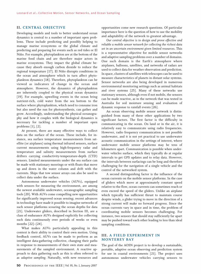
Autonomous underwater gliders are buoyancy-driven,

endurance vehicles. They use pumping systems to control

their net buoyancy so that they can move up and down inthe ocean. Fixed wings and tail give them lift and help

them to follow sawtooth trajectories in the vertical plane.

Gliders can actively redistribute internal mass to control

attitude. For heading control, they shift mass to roll, bank,

and turn (Spray) or use a rudder (Slocum). During the

field experiment, the gliders were configured to maintain a

fixed velocity relative to the flow. Their effective forward

speed was approximately 25 cm/s (Spray) to 35 cm/s(Slocum); this is of the same order as the stronger currents

in and around Monterey Bay. Accordingly, the gliders do

not make progress in certain directions when the currents

are too strong.

The Spray gliders, rated to 1500 m depth and operated

to 400 m and sometimes 750 m during summer 2003, were

deployed in deep water, traveling as far as 100 km offshore.

The Slocum gliders, operated to 200 m depth, were

deployed closer to the coast. The gliders surfaced at regular

intervals (although not synchronously) to get GPS fixes for

navigation, to send data collected back to shore and to

receive updated mission commands. The communicationto and from the shore computers, via Iridium satellite and

ethernet, was the only opportunity for communication

Bbetween[ gliders; the gliders were not equipped with

means to communicate while they were underwater.

On a typical single battery cycle, the Slocum gliders

performed continuously for up to two weeks between

deployment and recovery while the Spray gliders remained

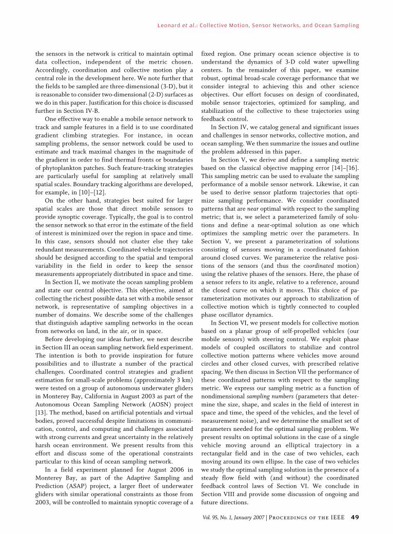
in the water for the entire experiment (about five weeks).Collectively, the gliders delivered a remarkably plentiful

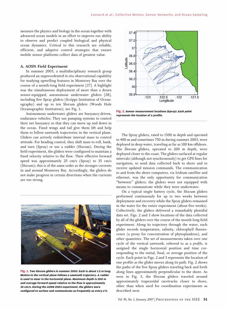
data set. Figs. 2 and 3 show locations of the data collected

by all of the gliders over the course of the month-long field

experiment. Along its trajectory through the water, each

glider records temperature, salinity, chlorophyll fluores-

cence (a proxy for concentration of phytoplankton), and

other quantities. The set of measurements taken over one

cycle of the vertical sawtooth, referred to as a profile, isassigned the single horizontal position and time cor-

responding to the initial, final, or average position of the

cycle. Each point in Figs. 2 and 3 represents the location of

one profile as the glider moves along its path. Fig. 2 shows

the paths of the five Spray gliders traveling back and forth

along lines approximately perpendicular to the shore. As

seen in Fig. 3, the Slocum gliders traveled around

approximately trapezoidal racetracks closer to shore,other than when used for coordination experiments as

described next.

Fig. 1. Two Slocum gliders in summer 2003. Each is about 1.5 m long.

Motion in the vertical plane follows a sawtooth trajectory. A rudder

is used to steer in the horizontal plane. Maximum depth is 200 m

and average forward speed relative to the flow is approximately

35 cm/s. During the AOSN 2003 experiment, the gliders were

configured to surface and communicate as frequently as every 2 h.

Fig. 2. Sensor measurement locations (Spray). Each point

represents the location of a profile.



B. Cooperative Control Sea TrialsIn this section we summarize results of sea trials, run as

part of the field experiment, with small fleets of Slocum

underwater gliders controlled in formations [13]. The

focus was on relatively small scales in the region (on the

order of 3 km) and feature tracking capabilities of mobile

sensor networks. The sea trials were aimed at demonstrat-ing strategies for cooperative control and gradient es-

timation of scalar sampled fields using a mobile sensor

network comprised of three gliders in a strong flow field

with limited communication and feedback.

The control strategy was derived from the virtual bodyand artificial potential (VBAP) multivehicle control meth-

odology presented in [29]. VBAP is a general strategy for

coordinating the translation, rotation, and dilation of agroup of vehicles and can be used in missions such as

gradient climbing in a scalar, environmental field. A

virtual body is a collection of moving reference points with

dynamics that are computed centrally and broadcast to

vehicles in the group. Artificial potentials are used to

couple the dynamics of vehicles and a virtual body so that

desired formations of vehicles and a virtual body can be

stabilized. Each vehicle uses a control law that derivesfrom the gradient of the artificial potentials; therefore,

each vehicle must have available the position of at least the

nearest neighboring vehicles and the nearest reference

points on the virtual body. If sampled measurements of a

scalar field can be communicated to a central computer,

the local gradients of a scalar field can be estimated.

Gradient climbing algorithms can also prescribe virtual

body direction. For example, the virtual body (andconsequently the vehicle group) can be directed to head

for the coldest water when temperature gradient estimates

computed from vehicle measurements are available. The

speed of the virtual body is controlled to ensure stabilityand convergence of the vehicle formation.

The control theory and algorithms described in [29]

depend upon a number of ideal assumptions on the opera-

tion of the vehicles in the group, including continuous

communication and feedback. Since this was not the case in

the operational scenario of the field experiment, a number

of modifications were made. Details of the modifications

are described in [30]; these include accommodation ofconstant speed of gliders, relatively large ocean currents,

waypoint tracking routines, communication only when

gliders surface (asynchronously), and other latencies.

For the Slocum vehicles, each glider has on-board low-

level control for heading and pitch which enables it to

follow waypoints [31]. A waypoint refers to a vertical

cylinder in the ocean with given radius and position. When

a sequence of waypoints is prescribed, the glider follows thewaypoints by passing through each of the corresponding

cylinders in the prescribed sequence using its heading

control. Heading control requires not only that the glider

know the prescribed waypoint sequence, but also that it can

measure (or estimate) its own position and heading.

Heading is measured on-board the glider (as is pitch and

roll). Depth and vertical speed are estimated from pressure

measurements. From these measurements and somefurther assumptions, the glider estimates its horizontal

speed. Position is then computed by integration, using the

most recent GPS fix as the initial condition. This deduced

reckoning approach also makes use of an estimate of

average flow, computed from the error on the surface

between the glider’s GPS and its dead-reckoned position.

In the cooperative control sea trials of 2003, the gliders

used their low-level control to follow waypoints as perusual; however, the waypoint sequences were updated

every 2 h using the VBAP control strategy for coordination.

VBAP was run on a simulation of the glider group using the

most recent GPS fixes and average flow measurements as

initial conditions. The trajectories generated by VBAP

were then discretized into waypoint lists which were

transmitted to the gliders when they surfaced. The ap-

proach is discussed further in [13], [30].On August 6, 2003, a sea trial was run in which three

Slocum gliders were commanded to move northwest in

an equilateral triangle with inter-glider distance equal to

3 km. The desired path of the center of mass of the vehicle

group was pre-planned. The trial was run for 16 h, with

gliders surfacing every 2 h (although not at the same time).

The orientation of the group was unrestricted in the first

half of the sea trial and constrained in the second half ofthe sea trial so that one edge of the triangle would always

be normal to the path of the center of mass of the group.

Snapshots of glider formations as well as glider group

estimates of the negative temperature gradient are shown

in Fig. 4 for the August 6, 2003 sea trial. The group stayed

in formation and moved along the desired track despite

relatively strong currents. Further, the negative gradient

Fig. 3. Sensor measurement locations (Slocum). Each point

represents the location of a profile.



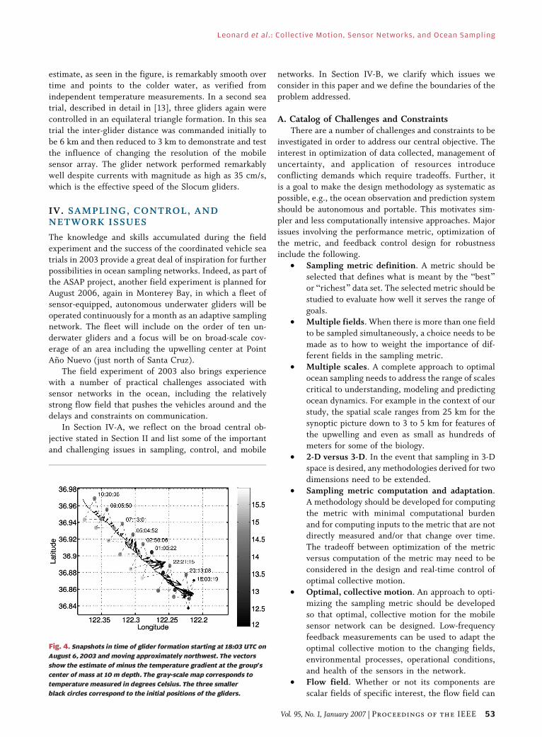
estimate, as seen in the figure, is remarkably smooth overtime and points to the colder water, as verified from

independent temperature measurements. In a second sea

trial, described in detail in [13], three gliders again were

controlled in an equilateral triangle formation. In this sea

trial the inter-glider distance was commanded initially to

be 6 km and then reduced to 3 km to demonstrate and test

the influence of changing the resolution of the mobile

sensor array. The glider network performed remarkablywell despite currents with magnitude as high as 35 cm/s,

which is the effective speed of the Slocum gliders.

IV. SAMPLING, CONTROL, ANDNETWORK ISSUES

The knowledge and skills accumulated during the fieldexperiment and the success of the coordinated vehicle seatrials in 2003 provide a great deal of inspiration for furtherpossibilities in ocean sampling networks. Indeed, as part ofthe ASAP project, another field experiment is planned forAugust 2006, again in Monterey Bay, in which a fleet ofsensor-equipped, autonomous underwater gliders will beoperated continuously for a month as an adaptive samplingnetwork. The fleet will include on the order of ten un-derwater gliders and a focus will be on broad-scale cov-erage of an area including the upwelling center at PointAno Nuevo (just north of Santa Cruz).

The field experiment of 2003 also brings experiencewith a number of practical challenges associated withsensor networks in the ocean, including the relativelystrong flow field that pushes the vehicles around and thedelays and constraints on communication.

In Section IV-A, we reflect on the broad central ob-

jective stated in Section II and list some of the important

and challenging issues in sampling, control, and mobile

networks. In Section IV-B, we clarify which issues weconsider in this paper and we define the boundaries of the

problem addressed.

A. Catalog of Challenges and ConstraintsThere are a number of challenges and constraints to be

investigated in order to address our central objective. The

interest in optimization of data collected, management of

uncertainty, and application of resources introduceconflicting demands which require tradeoffs. Further, it

is a goal to make the design methodology as systematic as

possible, e.g., the ocean observation and prediction system

should be autonomous and portable. This motivates sim-

pler and less computationally intensive approaches. Major

issues involving the performance metric, optimization of

the metric, and feedback control design for robustness

include the following.• Sampling metric definition. A metric should be

selected that defines what is meant by the Bbest[or Brichest[ data set. The selected metric should be

studied to evaluate how well it serves the range of

goals.

• Multiple fields. When there is more than one field

to be sampled simultaneously, a choice needs to be

made as to how to weight the importance of dif-ferent fields in the sampling metric.

• Multiple scales. A complete approach to optimal

ocean sampling needs to address the range of scales

critical to understanding, modeling and predicting

ocean dynamics. For example in the context of our

study, the spatial scale ranges from 25 km for the

synoptic picture down to 3 to 5 km for features of

the upwelling and even as small as hundreds ofmeters for some of the biology.

• 2-D versus 3-D. In the event that sampling in 3-D

space is desired, any methodologies derived for two

dimensions need to be extended.

• Sampling metric computation and adaptation.

A methodology should be developed for computing

the metric with minimal computational burden

and for computing inputs to the metric that are notdirectly measured and/or that change over time.

The tradeoff between optimization of the metric

versus computation of the metric may need to be

considered in the design and real-time control of

optimal collective motion.

• Optimal, collective motion. An approach to opti-

mizing the sampling metric should be developed

so that optimal, collective motion for the mobilesensor network can be designed. Low-frequency

feedback measurements can be used to adapt the

optimal collective motion to the changing fields,

environmental processes, operational conditions,

and health of the sensors in the network.

• Flow field. Whether or not its components are

scalar fields of specific interest, the flow field can

Fig. 4. Snapshots in time of glider formation starting at 18:03 UTC on

August 6, 2003 and moving approximately northwest. The vectors

show the estimate of minus the temperature gradient at the group’s

center of mass at 10 m depth. The gray-scale map corresponds to

temperature measured in degrees Celsius. The three smaller

black circles correspond to the initial positions of the gliders.



directly influence sampling performance because itcan push the sensors around and prevent them from

carrying out optimal sampling strategies. Accord-

ingly, strong flow fields must be considered in the

design of optimal, collective motion. A methodol-

ogy to exploit available estimates or predictions of

the flow field is of significant interest.

• Feedback control of collective motion. Relative-

ly high rate feedback control strategies thatstabilize optimal collective motion are necessary

to ensure robustness of optimal sampling strategies

not only with respect to the external flow field but

also to other disturbances and uncertainties in the

environment.

Additionally, there are a number of issues associated

with the sensor platforms themselves and their network

operation. A list of these issues in the case of glidersfollows.

• Constant speed. Strategies for collective motion

must take into account that gliders effectively op-

erate at constant speed (relative to the flow field).

Otherwise, patterns may be designed that are not

realizable. Gliders can also be operated as virtual

moorings, which may be applicable to the adaptive

sampling problem but is not considered here.• Transit and irregular events. There will be a

significant period of time when mobile sensors are

Bin transit,[ meaning that they are on their way

between optimal sampling patterns. For example,

when gliders are first deployed they should transit

to locations where they will initiate their optimal

strategy. However, gliders are slow and the period

of time it will take to get to these locations may besignificant. Therefore, their paths should be

designed both to optimize sampling during transit

and to minimize transit time. Similar strategies

should be developed in case a mobile sensor

encounters a region it must avoid (e.g., due to

fishing), is taken out of the water for whatever

reason, experiences a debilitating failure, etc.

• Heterogeneous groups. In case mobile sensors inthe network differ in speed, endurance, sensors,

etc., methodologies should be developed to exploit

the differing strengths and potential roles of the

sensors in the network. For instance, slow, high-

endurance vehicles might be more useful for larger

scales whereas fast, low-endurance vehicles might

serve better collecting data over smaller scales.

• Extending lifetime of sensors. Underwatergliders are designed to be high-endurance vehicles,

a central objective being to collect data continu-

ously over weeks or even months at a time.

Accordingly, keeping energy use to a minimum is

critical. This implies also keeping volume (and

therefore mass) to a minimum. There is a direct

tradeoff here with improving sensing, navigation,

communication, and control. For example, com-munication on the ocean surface makes possible

coordinated control of the sensors. However,

surfacings that are too frequent can be costly in

terms of energy expenditure and loss of time

collecting data, whereas surfacings that are too

infrequent yield very long feedback sampling

periods which can diminish the performance and

robustness of the control.• Communication. Communication between gliders

is done above the surface via a central data hub.

Coordinated control strategies for the network of

sensors that were originally designed assuming

continuous control will need to be revisited. Since

minimizing the frequency of surfacings is desirable

to minimize energy and maximize time spent

collecting undersea data and minimize exposure, itis of interest to determine the maximum tolerable

feedback sampling period that does not degrade

overall sampling performance as a function of the

magnitude of disturbances such as flow.

• Asynchronicity. Strategies will need to accommo-

date asynchronicity in time of surfacing and

communication. Because the gliders will not

surface at the same time, information communi-cated to a glider about any of the other gliders will

necessarily be old.

• Latencies. It may not always be possible to close

the feedback loop on the surface. For example, in

the sea trials of 2003, described in Section III-B,

data retrieved from a glider at its surfacing could

not be used in the waypoint update to the glider at

that same surfacing. Instead the data was used tocompute new instructions communicated to the

glider at the next surfacing. This introduces

significant delays that need to be accommodated.

• Computing. While low-level control is computed

on board the gliders, coordinated control of the

network is computed on the central shore com-

puter where inter-glider communication occurs.

Possibilities for further exploiting on-board com-putation and local measurements should be

investigated.

B. Problem DefinitionIn this paper we address sampling a single time- and

space-varying scalar field, like temperature, using mobile

platforms like gliders. Emphasis is on how to operate such

vehicles, either singly or in coordinated fleets, to providethe most information about this field. Since the main

operational control is over course and speed, we focus on

mapping a single 2-D horizontal field. Ultimately the data

would be used to describe the 3-D field either directly by

analysis of 3-D data or indirectly by assimilating data into

high-resolution dynamical ocean models [32]–[34]. How-

ever, because ocean scales are similar through the upper



water column and horizontal position is the main controlvariable, the 2-D problem suffices.

To measure how well a given sampling array describes

the variable of interest, we adopt a simple metric based

on objective analysis (linear statistical estimation based

on specified field statistics). This metric (defined in

Section V-A) specifies the statistical uncertainty of the

model as a function of where and when the data is taken.

Since reduced uncertainty implies better measurementcoverage, we also refer to this as a coverage metric. In

ongoing work [2], [35]–[37], information that can be

inferred from a dynamical model is included in the metricused to control vehicles.

We frame the optimal collective motion problem and

define our approach to design of a (near) optimal mobile

sensor network in Section V. By near optimal solutions, we

mean that we optimize over a parameterized family of

structured solutions. For example, we consider a family of

closed curves parameterized by number, location, dimen-

sion, and shape as well as the relative phases of the vehiclesmoving around these curves. This parameterization is

discussed in Section V-D. The relative phases provide a

low-dimensional parameterization of relative position of

the vehicles and they make a connection between the

optimized trajectories and the coupled phase oscillator

models that we use in our coordinated control law.

We pay particular attention to gliders moving around

ellipses for several reasons. First, the various periodictrajectories appropriate for oceanographic sampling (e.g.,

moving back and forth on a line or around a trapezoid as

shown in Figs. 2 and 3 from the 2003 AOSN field

experiment) can be reasonably approximated with ellipses

by tuning the eccentricity. Second, ellipses are minimally

parameterized, smooth shapes for which we have devel-

oped a control theoretic framework. In [38], we have

generalized our control framework to a class of curvesknown as superellipses, which includes circles, ellipses and

rounded rectangles. By considering superellipses and

optimizing over the parameters that define them, we aim

to go beyond the hand-crafted trajectories of previousexperience, to automate the design, adaptation and control

of sensor patterns that yield maximally information rich

data sets.

In the case of gliders moving with constant speed

around circles, the difference in heading for any pair of

gliders can be interpreted as the relative phase of that pair

of gliders. For example, if for a pair of gliders moving

around the same circle, the difference in heading is180 degrees, then the relative phase is 180 degrees and

the gliders are always at antipodal points on the circle.

For ellipses, the relative phase is not necessarily

equivalent to the relative heading and so an

alternate phase variable based on arc length along

the desired curve can be used.

In Section VI, we present feedback control

laws that stabilize these kinds of collectivemotions for gliders moving at constant (unit)

speed on the plane. We focus on the case that

there may be multiple ellipses and multiple

vehicles per ellipse. The objective is to ensure

that gliders move around their (optimally located,

oriented, and sized) ellipses with optimal relative

phases. In Section VII, we compute and study

optimal solutions and we discuss robustness of thesolutions with respect to the coverage metric. We

also investigate the influence of the flow field on

the design and control of optimal sampling trajectories.

In this paper, we assume a homogeneous group of

mobile sensors. We do not address the issue of transit and

irregular events; preliminary results on minimal time and

minimal energy glider paths computed using forecasts of

ocean flow fields are presented in [39]. We also do notaddress the problems in communication, asynchronicity,

latency, and computing described above. In [13] and [30] it

is discussed how these issues were handled in AOSN 2003.

In [40], a control law is presented that explores extended

sensing, computing, and control onboard a glider. In this

paper, we let each sensor compute its own control law

locally and we assume continuous feedback control with

continuous communication without delay or asynchroni-city. Because communication is not limited to neighboring

gliders in the operational scenario, we assume an all-to-all

interconnection topology.

A number of the issues listed in Section IV-A re-

main important open problems and are the subject of

ongoing work.

V. SAMPLING METRIC AND OPTIMALITY

A. Sampling MetricIn this section, we derive a metric to quantify how

well an array of gliders samples a given region. Recall that

the data will be assimilated in ocean models. Therefore,

the metric should reflect how a particular data set reduces

By considering superellipses andoptimizing over the parametersthat define them, we aim to gobeyond the hand-craftedtrajectories of previous experi-ence, to automate the design,adaptation and control of sensorpatternsthat yield maximally informationrich data sets.



the error in a model. This notion is necessarily dependenton the specific model or assimilation scheme used. During

AOSN 2003, the data was assimilated in several high-

resolution ocean models [32]–[34] and the performance

of the sampling array was similar for each. Since reliable

nowcasts and forecasts of the ocean require concurrent

ocean models mutually validating their results and the data

requirements of these models are similar, it is natural to

derive the performance metric on a simpler, more generalassimilation scheme. This approach also has the advantage

of avoiding the complexity and computational effort re-

quired to study specific high-resolution models [41], [42].

To compute our metric we need only a background covariancefunction to describe the field and the locations and timescorresponding to where and when the data was collected; themeasurements and forecast of the field are not needed.

We consider a simple data assimilation scheme calledobjective analysis2 (see e.g., [43], [44]). In this framework,

the scalar field (e.g., temperature, salinity) observed at a

point r and at a time t is viewed as a random variable

Tðr; tÞ or an ensemble of possible realizations. The

algorithm provides an estimate for the average and the

error variance of this estimate assuming we have an a prioridescription of the field, usually the mean �T and the

covariance B of fluctuations around the mean

�Tðr; tÞ ¼E Tðr; tÞ½ � (1)

Bðr; t; r0; t0Þ ¼E Tðr; tÞ � �Tðr; tÞ½ �½� Tðr0; t0Þ � �Tðr0; t0Þ½ �� (2)

where E½� represents the expected value of a randomvariable. The Bdiagonal[ elements Bðr; t; r; tÞ contain the

variance of Tðr; tÞ around its expected value �Tðr; tÞ. We

note that the assumed value of �T is needed for the

estimate of the field but not for the error variance of this

estimate and therefore not for the performance metric

that we will define.

The data collected by the gliders is a sequence of Pmeasurements Tk at discrete points ðrk; tkÞ, k ¼ 1; . . . ; P.Objective analysis consists in finding an estimate Tðr; tÞ of

the field Tðr; tÞ as a linear combination of all the data

Tðr; tÞ ¼ �Tðr; tÞ þXP

k¼1

�kðr; tÞ Tk � �Tðrk; tkÞ½ � (3)

where the P coefficients �k minimize the least square

uncertainty of Tðr; tÞ. While the estimate for a pair ðr; tÞcan be computed independently of others, the coefficients

�kðr; tÞ minimize the mean square error integrated overthe region and period of interest

Zdr

Zdt E Tðr; tÞ � Tðr; tÞ

� �Tðr; tÞ � Tðr; tÞ� ��

: (4)

The optimal coefficients [43] are

�kðr; tÞ ¼XP

l¼1

Bðr; t; rl; tlÞðC�1Þkl (5)

where C�1 is the inverse of the P � P covariance matrix of

the data Tk. When the measurement noise is uniform anduncorrelated, ðCÞkl ¼ n�kl þ Bðrk; tk; rl; tlÞ, where �kj is the

Dirac delta and n is the noise variance. The covariance of

the error in the estimate T is obtained by direct substitution

of (5) and (3) in the integrand of (4) and is given by

Aðr; t; r0; t0Þ ¼� E Tðr; tÞ � Tðr; tÞ� �

Tðr; tÞ � Tðr; tÞ� ��

¼ Bðr; t; r0; t0Þ �XP

k;l¼1

Bðr; t; rk; tkÞðC�1Þkl

� Bðrl; tl; r0; t0Þ: (6)

The quantity Aðr; t; r; tÞ, the variance of T around the

estimate T, is also known as the a posteriori error. An

extensive analysis of the assimilation scheme, equations,

and generalizations (e.g., multivariate, discrete, nonsta-

tionary systems) can be found in [43] and [44].

Because estimation errors of a hypothetical samplingarray are determined by the statistics of the field noise,

Aðr; t; r; tÞ can be used as a quantitative measure of the

impact of a sequence of measurements on knowledge of the

field and allows a priori design of effective sampling arrays

[16]. In this paper, the integral of Aðr; t; r; tÞ over the domain

� ¼�Z

dr

Zdt Aðr; t; r; tÞ (7)

equivalent to (4) evaluated at the optimal T, is elected as the

sampling performance metric to compare and optimize

sampling strategies. Substitution of (6) in (7) gives

� ¼Z

dr

Zdt Bðr; t; r; tÞ

�XP

k;l¼1

Bðr; t; rk; tkÞðC�1ÞklBðrl; tl; r; tÞ!: (8)

2Objective analysis is also commonly referred to as optimalinterpolation. It was originally developed by Eliassen et al. [14] in 1954and independently reproduced and popularized by Gandin [15] in 1963.



Note that this metric depends only on the covariancefunction B, the noise variance and the measurement

locations and times, rk and tk.

B. Ocean StatisticsThe coverage metric defined in (8) requires specifica-

tion of the term Bðr; t; r0; t0Þ, an estimate of the

background statistics. It represents the estimated statistics

of the ocean before data assimilation. The diagonalelements Bðr; t; r; tÞ describe our confidence in the initial

state. The nondiagonal elements represent the covariance

between points at different locations and times. They are

closely related to the correlation length and the correlation

time in the domain [16].

The metric in (8) has a broad range of application and

can be used with any positive-definite covariance function

Bðr; t; r0; t0Þ. For the purpose of illustrating the use of the

metric, we assume that the background covariance isgiven by

Bðr; t; r0; t0Þ ¼� �0e�kr�r0k2

�2 �jt�t0 j2�2 : (9)

The parameters � and � are the a priori spatial and

temperature decorrelation scales; because (9) fixes the

structure of the term B, � and � can be viewed as inputs to

the objective analysis algorithm. In this paper, we use

� ¼ 25 km and � ¼ 2:5 days; these values were deter-

mined empirically using glider data from Monterey Bay

during AOSN 2003 [28]. Notice that the scaling factor �0

has no effect on the sampling paths, provided that the

measurement noise n is scaled by the same factor. This fact

is discussed and exploited in Section VII.

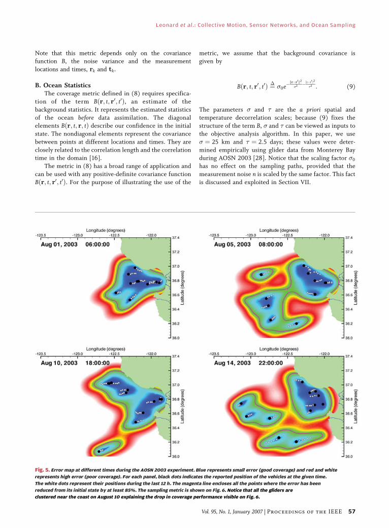
Fig. 5. Error map at different times during the AOSN 2003 experiment. Blue represents small error (good coverage) and red and white

represents high error (poor coverage). For each panel, black dots indicates the reported position of the vehicles at the given time.

The white dots represent their positions during the last 12 h. The magenta line encloses all the points where the error has been

reduced from its initial state by at least 85%. The sampling metric is shown on Fig. 6. Notice that all the gliders are

clustered near the coast on August 10 explaining the drop in coverage performance visible on Fig. 6.



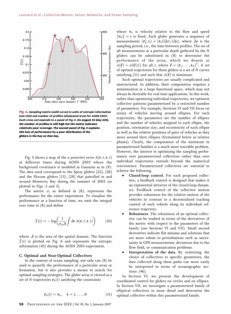
Fig. 5 shows a map of the a posteriori error Aðr; t; r; tÞat different times during AOSN 2003 where the

background covariance is modeled as Gaussian as in (9).

The data used correspond to the Spray gliders [22], [28]

and the Slocum gliders [13], [28] that patrolled in andaround Monterey Bay during the summer of 2003 (as

plotted in Figs. 2 and 3).

The metric �, as defined in (8), represents the

performance for the entire experiment. To visualize the

performance as a function of time, we omit the integral

over time in (8) and define

IðtÞ ¼ � log1

�0A

Zdr Aðr; t; r; tÞ

� �(10)

where A is the area of the spatial domain. The function

IðtÞ is plotted on Fig. 6 and represents the entropic

information [45] during the AOSN 2003 experiment.

C. Optimal and Near-Optimal CollectivesIn the context of ocean sampling, not only can (8) be

used to quantify the performance of a particular array or

formation, but it also provides a means to search for

optimal sampling strategies. The glider array is viewed as a

set of N trajectories rkðtÞ satisfying the constraints

_rkðtÞ ¼ vk; k ¼ 1; . . . ;N (11)

where vk is velocity relative to the flow and speedkvkk ¼ v is fixed. Each glider generates a sequence of

measurements ðrlk; tlÞ ¼ ðrkðl�tÞ; l�tÞ, where �t is the

sampling period, i.e., the time between profiles. The set of

all measurements at a particular depth gathered by the Ngliders can be substituted in (8) to determine the

performance of the array, which we denote as

�ð~rÞ ¼ �ð~rðtÞÞ for all t, where ~r ¼ ðr1; . . . ; rNÞT. A set

of optimal trajectories for these gliders is a set of N curvessatisfying (11) and such that �ð~rÞ is minimum.

Such optimal trajectories are usually complicated and

unstructured. In addition, their computation requires a

minimization in a large functional space, which may not

always be desirable for real-time applications. In this work,

rather than optimizing individual trajectories, we optimize

collective patterns parameterized by a restricted number

of parameters. For example, Sections VI and VII focus onarrays of vehicles moving around ellipses. For such

trajectories, the parameters are the number of ellipses

and the number of vehicles assigned to each ellipse, the

position, orientation size, and eccentricity of each ellipse

as well as the relative positions of pairs of vehicles as they

move around their ellipses (formulated below as relative

phases). Clearly, the computation of the minimum in

parameterized families is a much more tractable problem.However, the interest in optimizing the sampling perfor-

mance over parameterized collectives rather than over

individual trajectories extends beyond the numerical

convenience. Parameterized collectives are essential to

achieve the following.

• Closed-loop control. For each proposed collec-

tive, a feedback control is designed that makes it

an exponential attractor of the closed-loop dynam-ics. Feedback control of the collective motion

provides robustness for the relative motion of the

vehicles in contrast to a decentralized tracking

control of each vehicle along its individual ref-

erence trajectory.

• Robustness. The robustness of an optimal collec-

tive can be studied in terms of the derivatives of

the metric with respect to the parameters of thefamily (see Sections VI and VII). Small second

derivatives indicate flat minima and solutions that

are more robust to perturbations such as uncer-

tainty in GPS measurements, deviations due to the

flow field, or communication problems.

• Interpretation of the data. By restricting the

choice of collectives to specific geometries, the

data collected along these paths can more easilybe interpreted in terms of oceanographic sec-

tions [46].

In Section VI, we present the development of

coordinated control for gliders on circles and on ellipses.

In Section VII, we investigate a parameterized family of

elliptical collectives in more detail and determine the

optimal collective within this parameterized family.

Fig. 6. Sampling metric (solid curve) in units of entropic information

[see (10)] and number of profiles (shadowed area) for AOSN 2003.

Each cross corresponds to a panel of Fig. 5. On August 10 (day 223),

the number of profiles is still high but the metric indicates

relatively poor coverage. The second panel of Fig. 5 explains

this loss of performance by a poor distribution of the

gliders in the bay on that day.



D. Parameterization of CollectivesParameterized families of collectives over closed

curves involving the least number of parameters are

circles. If we specialize to circles, the optimal parameters

to be computed are the number of circles, the number of

gliders per circle, the origin and radius of each circle, and

the relative positions of the gliders on their respective

circles. The relative position of two gliders moving

around the same circle can be represented by thedifference in their headings; this difference is fixed since

the gliders move at constant speed. The difference in the

headings is equal to the relative phase of the gliders

around the circle. To see this, suppose the gliders move at

unit speed around a single circle of radius 0 ¼ j!0j�1

and centered at the origin. The position of the kth glider

at time t is rkðtÞ ¼ 0ðcosð!0t þ �kÞ; sinð!0t þ �kÞÞ,where �k is the phase of the kth glider. The derivativeof rk with respect to time is _rk ¼ sgnð!0Þð�sinð!0t þ�kÞ; cosð!0t þ �kÞÞ. The velocity of the glider can also be

expressed as _rk ¼ ðcos �k; sin �kÞ, where �k is the glider’s

heading angle. By equating these two expressions for _rk,

we get !0t þ �k þ sgnð!0Þ =2 ¼ �k. Thus, the relative

heading of two vehicles is equal to their relative phase, i.e.,

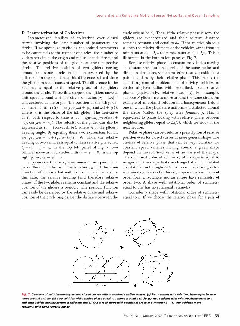
�j � �k ¼ �j � �k. In the top left panel of Fig. 7, two

vehicles move around circles with �2 � �1 ¼ 0. In the topright panel, �2 � �1 ¼ .

Suppose now that two gliders move at unit speed about

two different circles, each with radius 0 and the same

direction of rotation but with noncoincident centers. In

this case, the relative heading (and therefore relative

phase) of the two gliders remains constant and the relative

position of the gliders is periodic. The periodic function

can easily be described by the relative phase and relativeposition of the circle origins. Let the distance between the

circle origins be d0. Then, if the relative phase is zero, thegliders are synchronized and their relative distance

remains constant and equal to d0. If the relative phase is

, then the relative distance of the vehicles varies from its

minimum at d0 � 20 to its maximum at d0 þ 20. This is

illustrated in the bottom left panel of Fig. 7.

Because relative phase is constant for vehicles moving

at constant speed around circles of the same radius and

direction of rotation, we parameterize relative position of apair of gliders by their relative phase. This makes the

stabilizing control problem one of driving vehicles to

circles of given radius with prescribed, fixed, relative

phases (equivalently, relative headings). For example,

suppose N gliders are to move around the same circle. An

example of an optimal solution in a homogeneous field is

one in which the gliders are uniformly distributed around

the circle (called the splay state formation). This isequivalent to phase locking with relative phase between

neighboring gliders equal to 2 =N, which we study in the

next section.

Relative phase can be useful as a prescription of relative

position even for closed curves of more general shape. The

choices of relative phase that can be kept constant for

constant speed vehicles moving around a given shape

depend on the rotational order of symmetry of the shape.The rotational order of symmetry of a shape is equal to

integer L if the shape looks unchanged after it is rotated

about its center by angle 2 =L. For example, a hexagon has

rotational symmetry of order six, a square has symmetry of

order four, a rectangle and an ellipse have symmetry of

order two. A shape with rotational order of symmetry

equal to one has no rotational symmetry.

Consider a shape with rotational order of symmetryequal to L. If we choose the relative phase for a pair of

Fig. 7. Cartoons of vehicles moving around closed curves with prescribed relative phases. (a) Two vehicles with relative phase equal to zero

move around a circle. (b) Two vehicles with relative phase equal to move around a circle. (c) Two vehicles with relative phase equal to

and each vehicle moving around a different circle. (d) A closed curve with rotational order of symmetry L ¼ 4. Four vehicles move

around it with fixed relative phase.



gliders moving at constant speed around the shape to be aninteger multiple of 2 =L, the relative phase will remain

constant. An example for L ¼ 4 is shown in Fig. 7. In the

case of circles, as discussed above, any relative phase can

be selected. In the case of ellipses, only two choices of

relative phase can be selected; these are either relative

phase equal to zero or equal to , when the gliders are

synchronized or antisynchronized, respectively, as they

move around a single ellipse or up to N identical ellipseswith noncoincident centers.

In Section VI, we describe steering control laws for

stabilization of gliders to circles and ellipses with phase

locking.

VI. COORDINATED CONTROL

This section describes feedback control laws that stabilizecollective motion of a planar model of autonomous

vehicles moving at constant speed. Following Section V,

we consider vehicles moving around closed curves with

given, fixed relative phases. As described in Section V-D,

relative phases determine, in part, the relative positions of

the vehicles. In the case of collective motion around circles

of equal radius and direction of rotation, the relative phase

is identical to relative heading and is also constant. Formore general shapes, prescribed relative phases are chosen

as an integer multiple of 2 =L where L is the rotational

order of symmetry of the shape. For example, in the case of

coordinated motion of gliders around ellipses, L ¼ 2 and

we design stabilizing controllers that fix relative phases to

0 or . This restriction can be relaxed using an alternate

definition of relative phase based on arc length along the

desired curve [38].Each glider is modeled as a point mass with unit mass,

unit speed, and steering control. We first provide a feed-

back control law that stabilizes circular motion of the

group of vehicles about its center of mass. This control law

depends on the relative position of the vehicles. Next, we

address the problem of stabilizing the relative phases of

the circling vehicles. An additional control term, de-

pending only on the relative headings of the vehicles,stabilizes symmetric patterns of the vehicles in the circu-

lar formation.

As long as the feedback control is a function only of the

relative positions and headings of the vehicles, the system

dynamics are invariant to rigid rotation and translation of

the whole vehicle group in the plane. This corresponds to

the symmetry group, SEð2Þ ¼ SOð2Þ � R2 � S1 � R2,

where � is the semi-direct product. Here, SOð2Þ ¼ fX 2R2�2jXTX ¼ I; detðXÞ ¼ 1g is the special orthogonal group

in the plane and describes the space of all 2-D rotations.

SOð2Þ is equivalent to S1, the one-dimensional sphere or

circle, since there is a one-to-one relationship between

rotations in the plane and angles in ½0; 2 Þ. SEð2Þ is the

special Euclidean group in the plane and describes the

space of all possible rigid rotations and translations in

the plane. We show how breaking this symmetry, i.e., byintroducing a control term that depends on the position

and/or orientation of the group as a whole, can lead to

useful variations on circular formations. First, we intro-

duce a fixed beacon to break the R2 symmetry. Second, we

introduce a reference heading which breaks the S1 sym-

metry. In addition, we introduce interconnection topol-

ogies for the spacing and orientation coupling that

stabilize collective motion of coordinated subgroups ofvehicles. This includes the case in which there are

multiple circles with a different subgroup of vehicles

moving around each circle.

Finally, we describe a control law to stabilize collective

motion on more general shapes. More specifically, we

stabilize a single vehicle on an elliptical trajectory about a

fixed beacon. Additionally, we couple vehicles on separate

ellipses using their relative headings in order to synchro-nize the vehicle phases about each ellipse.

A. Circular ControlThe vehicle model that we study is composed of N

identical point-mass vehicles subject to planar steering

control. The vehicle model is

_rk ¼ vei�k

_�k ¼ uk; k ¼ 1; . . .N (12)

where rk ¼ xk þ iyk 2 C � R2 and �k 2 S1 are the posi-tion and heading of each vehicle, v is the vehicle speed

relative to the flow, and uk is the steering control input to

the kth vehicle. In this section, we assume unit vehicle

speed, i.e., v ¼ 1, and ignore the flow.

In Section V, the position rk of the kth vehicle is a

vector in R2. In this section, we exploit the isometry

between R2 and C and we view rk as an element of the

real3 vector space C. The real vector spaces C and CN giveus more flexibility in choosing an inner product.4 We

define the inner product by

hz1; z2i ¼ Re �z>1 z2

(13)

where �zT1 represents the conjugate transpose of z1 and

Refg is the real part of a complex number. We view z1 and

z2 as the elements of the real vector space CN (i.e.,

isomorphic to R2N), for which (13) is a valid inner product.

3By real vector space, we mean a vector space for which the field ofscalars is R. Complex vector spaces are defined with complex scalars. Forexample, CN is both a real and a complex vector space. In this paper, weconsider CN as a real vector space only.

4hz1; z2i ¼ Ref�z>1 z2g is not an inner product for the complex vectorspaces C because it violates sesquilinearity. However, it is a valid innerproduct for the real vector spaces C and CN .



For the sake of brevity, we often stack identicalvariables for each vehicle in a common vector. For

example, ~� ¼ ð�1; . . . �NÞT 2 TN contains all the headings

and~r ¼ ðr1; . . . rNÞT 2 CN contains all the positions.

To help understand the model (12), consider the

following two examples of constant control input. For

uk ¼ !0 6¼ 0, the vehicles travel on fixed circles of radius

0 ¼ j!0j�1. The sense of rotation is given by the sign of

!0. For uk ¼ !0 ¼ 0, each vehicle follows a straighttrajectory in the direction of the initial heading.

Due to the unit speed and unit mass assumptions, we

can relate the coherence of vehicle headings to the motion

of the group. Let the center of mass of the group be

R ¼ ð1=NÞPN

j¼1 rj. Also, let the order parameter p~� 2 C,

denote the centroid of the vehicle headings on the unit

circle in the complex plane. The order parameter is equiv-

alent to the velocity of the center of mass of the group, i.e.,

p~� ¼� 1

N

XN

k¼1

ei�k ¼ 1

N

XN

k¼1

_rk ¼ _R:

Notice that we have 0 � jp~�j � 1. We define a potential

function U1 by

U1ð~�Þ ¼N

2jp~�j

2: (14)

The gradient of U1 is given by

@U1

@�k¼ hiei�k ;p~�i; k ¼ 1; . . . ;N: (15)

Certain distinguished motions of the group correspond to

critical points of U1. For instance, U1ð~�Þ is maximum for

parallel motion of the group ð8k : �k ¼ �0Þ and minimum

when the center of mass is fixed ðp~� ¼ _R ¼ 0Þ. We refer

to solutions for which p~� ¼ _R ¼ 0 as balanced solutions

since the headings are distributed around the unit circle so

that the center of mass of the group is fixed. Letting~1 ¼ ð1; ; 1ÞT 2 RN, we use (15) to observe thathrU1;~1i ¼ hip~�;p~�i ¼ 0; this corresponds to the S1

rotational symmetry of the system since U1 is invariant

to rigid rotation of the vehicle headings.

To stabilize circular motion of the group about its

center of mass, we introduce a dissipative control law that

is a function of the relative positions rkj ¼ rk � rj. Let the

vector from the center of mass to vehicle k be~rk ¼ rk �R ¼ ð1=NÞ

PNj¼1 rkj. We propose to control

the vehicles using

uk ¼ !0 1 þ �h~rk; _rkið Þ; k ¼ 1; . . .N (16)

where � 9 0 is a scalar gain. For intuition regarding thecontrol law (16), note that for � ¼ 0, vehicle k will

undergo circular motion with radius j!0j�1 and direction

of rotation determined by the sign of !0. The gain �regulates the contribution to the control of a dissipation

term which drives vehicle k such that its velocity is

perpendicular to the vector from the center of mass of the

group. The dissipation term evaluates to zero for circular

motion around a fixed center of mass.The stability of the circular motion of the group about a

common point can be studied using standard Lyapunov

functions. Consider the function

Sð~r; ~�Þ ¼ 1

2

XN

k¼1

jei�k � i!0~rkj2; !0 6¼ 0 (17)

which has minimum zero for circular motion around the

center of mass with radius 0 ¼ j!0j�1 and direction of

rotation determined by the sign of !0. Differentiating

Sð~r; ~�Þ along the solutions of the vehicle model gives

_S ¼XN

k¼1

h!0~rk; _rkið!0 � ukÞ:

Therefore, using the circular control (16), we find that

_S ¼ ��XN

k¼1

h!0~rk; _rki2 � 0

and S is an acceptable Lyapunov function for this sys-

tem. Consequently, solutions converge to the largest in-variant set, �, for which _S ¼ 0. This yields the following

result.

Theorem 6.1: Consider the vehicle model (12) with the

circular control (16). All solutions converge to a circular

formation of radius 0 ¼ j!0j�1. Moreover, the relative

headings converge to an arrangement that is a critical point

of the potential U1ð~�Þ. In particular, balanced circularformations form an asymptotically stable set of relative

equilibria.

The technical details of the proof can be found in [47].

Notice that solutions in � have the dynamics_~� ¼ !0

~1, i.e.,

vehicles follow circles of radius j!0j�1. The set of balanced

circular solutions for which all circles are coincident

corresponds to the minimum of the potential Sð~r; ~�Þ.Simulations suggest that this set of equilibria has almost

global convergence.



B. Control of Relative HeadingsIf, in addition to the relative positions, we feed back the

relative headings of the vehicles, we can stabilize

particular phase-locked patterns or arrangements of the

vehicles in their circular formation. Let the potential Uð~�Þsatisfy hrU;~1i ¼ 0 so that it is invariant to rigid rotation

of all the vehicle headings. We combine the circular

control (16) with a gradient control term as follows:

uk ¼ !0 1 þ �h~rk; _rkÞð i � @U

@�k: (18)

The circular motion of the group in a phase-locked heading

arrangement is a critical point of Uð�Þ. The stability of themotion can be proved by showing the existence of a

Lyapunov function. For instance, take

Vð~r; ~�Þ ¼ �Sð~r; ~�Þ þ Uð~�Þ (19)

where Sð~r; ~�Þ is defined in (17). The time derivative of

Vð~r; ~�Þ along the solutions of the vehicle dynamics isgiven by

_V ¼XN

k¼1

�h!0~rk; _rki �@U

@�k

� �ð!0 � ukÞ: (20)

Substitution of the composite control (18) in (20) gives

_V ¼ �XN

k¼1

�h!0~rk; _rki �@U

@�k

� �2

� 0:

Therefore, solutions converge to the largest invariant set,

�, for which _V ¼ 0. A detailed proof can be found in [47]

and yields the following theorem.

Theorem 6.2: Consider the vehicle model (12) and a

smooth heading potential Uð�Þ that satisfies hrU;~1i ¼ 0.

The control law (18) enforces convergence of all solutions

to a circular formation of radius 0 ¼ j!0j�1. Moreover,

the relative headings converge to an arrangement that is a

critical point of the potential �U1 þ U. In particular, every

minimum of U for which U1 ¼ 0 defines an asymptotically

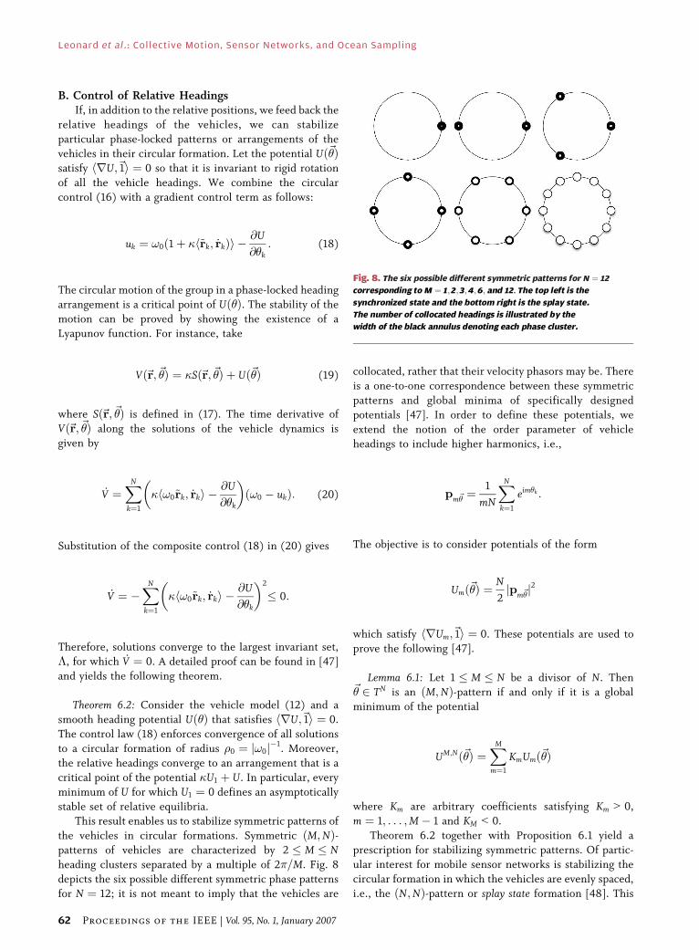
stable set of relative equilibria.This result enables us to stabilize symmetric patterns of

the vehicles in circular formations. Symmetric ðM;NÞ-patterns of vehicles are characterized by 2 � M � Nheading clusters separated by a multiple of 2 =M. Fig. 8

depicts the six possible different symmetric phase patterns

for N ¼ 12; it is not meant to imply that the vehicles are

collocated, rather that their velocity phasors may be. There

is a one-to-one correspondence between these symmetric

patterns and global minima of specifically designed

potentials [47]. In order to define these potentials, we

extend the notion of the order parameter of vehicle

headings to include higher harmonics, i.e.,

pm~� ¼1

mN

XN

k¼1

eim�k :

The objective is to consider potentials of the form

Umð~�Þ ¼N

2jpm~�j

2

which satisfy hrUm;~1i ¼ 0. These potentials are used to

prove the following [47].

Lemma 6.1: Let 1 � M � N be a divisor of N. Then~� 2 TN is an ðM;NÞ-pattern if and only if it is a global

minimum of the potential

UM;Nð~�Þ ¼XM

m¼1

KmUmð~�Þ

where Km are arbitrary coefficients satisfying Km 9 0,

m ¼ 1; . . . ;M � 1 and KM G 0.

Theorem 6.2 together with Proposition 6.1 yield a

prescription for stabilizing symmetric patterns. Of partic-

ular interest for mobile sensor networks is stabilizing the

circular formation in which the vehicles are evenly spaced,

i.e., the ðN;NÞ-pattern or splay state formation [48]. This

Fig. 8. The six possible different symmetric patterns for N ¼ 12

corresponding to M ¼ 1;2;3;4;6; and 12. The top left is the

synchronized state and the bottom right is the splay state.

The number of collocated headings is illustrated by the

width of the black annulus denoting each phase cluster.



formation is characterized by pm~� ¼ 0 for m ¼ 1; . . .N � 1and jpN~�j ¼ 1=N. Since pm~� ¼ 0 imposes two constraints

on the N � 1 relative phases for each m, we need only

specify the first bN=2c harmonics, where bN=2c is the

largest integer less than or equal to N=2 [47]. Conse-

quently, we define the splay state potential to be

UN;Nð~�Þ ¼ KXN

2b c

m¼1

Umð~�Þ; K 9 0: (21)

The splay state formation control law has the form (18)

with Uð~�Þ given by (21) and can be written

uk ¼ !0 1 þ �h~rk; _rkið Þ þ K

N

XN

j¼1

XbN=2c

m¼1

sin m�kj

m: (22)

A simulation of the splay state formation for N ¼ 12

vehicles is shown in Fig. 9. Twelve vehicles start from

random initial conditions and the controller (22) en-

forces convergence to a circular orbit with uniform spac-ing (i.e., the phase difference between adjacent vehicles

is 2 =12).

C. Planar Symmetry BreakingThe feedback control laws in Sections VI-A and VI-B

require only the relative positions and headings of the

vehicles and, consequently, they are invariant to rigid

translation and rotation in the plane. This corresponds tothe symmetry group, SEð2Þ � S1 � R2. In this section, we

introduce variations of these control laws that break the

translation and rotation symmetries. First, we break the R2

translation symmetry by stabilizing the circular formation

about a fixed beacon. Second, we break the S1 rotationalsymmetry by coupling the vehicles to a heading reference.

The position of the fixed beacon is referred to as

R0 2 C. The relative position from the beacon is defined

as ~rk ¼ rk �R0. A formal proof uses the Lyapunov

function Sð~r; ~�Þ defined in (17) with the new definition of~rk. Furthermore, Theorem 6.2 continues to hold for

circular motion about the fixed beacon [47]. That is, the

control (18) can be used to stabilize circular motion tothe set of heading arrangements that are critical points of

the potential Uð~�Þ, where hrU;~1 i ¼ 0. Clearly, this

applies to the splay state potential (21).

Next, we introduce a heading reference �0 where_�0 ¼ !0. Let uk, k ¼ 1; . . . ;N � 1 be given by (18), where

Uð~�Þ is a potential that satisfies hrU;~1i ¼ 0. The Nth

vehicle is coupled to the heading reference using

uN ¼ !0 1 þ �ð~rk; _rkÞð Þ � @U

@�kþ d sinð�0 � �NÞ (23)

where d 9 0. Critical points of Uð~�Þ that satisfy �N ¼ �0

define an asymptotically stable set [47]. To prove this

result, we use the composite Lyapunov function

Wð~r; ~�Þ ¼ Vð~r; ~�Þ þ d 1 � cosð�0 � �NÞð Þ

where Vð~r; ~�Þ is given by (19). The complete analysis canbe found in [47]. The set of circular formations that

minimizes Uð~�Þ and satisfies �N ¼ �0 are the global

minima of Wð~r; ~�Þ. For !0 ¼ 0, the control (23) can be

used to track piecewise linear trajectories [49].

D. Coordinated SubgroupsIn this section, we design control laws to coordinate

vehicles in subgroups using block all-to-all interconnectiontopologies. Here, the term Bblock[ refers to a subgroup of

vehicles and Ball-to-all[ refers to the interconnection

topology of that subgroup. It is assumed that the subgroups

are not interconnected unless otherwise stated. In other

words, the vehicles can be distributed among subgroups, in

which each subgroup corresponds to vehicles moving on a

different circle or ellipse. First, we introduce a block all-to-

all interconnection topology for the circular control termthat depends on the relative positions. This restriction on

the coupling yields stability of subgroups of vehicles in

separate circular formations. Similarly, block all-to-all

coupling applied to the gradient control term that depends

on relative headings yields heading arrangements within

subgroups of vehicles. We illustrate the use of block all-to-

all couplings on a scenario of practical interest. The

vehicles are divided into three subgroups that minimizethe splay state potential such that each subgroup is in a

splay state formation.

Fig. 9. Numerical simulation of the splay state formation starting

from random initial conditions using the control (22) with N ¼ 12,

!0 ¼ 0:1, � ¼ !0 and K ¼ !20. Each vehicle and its velocity is

illustrated by a black circle and an arrow. Note that the

center of mass of the group, illustrated by a crossed

circle, is fixed at steady-state.



We refer to each vehicle subgroup by its block indexb ¼ 1; . . . ; B, where B is the total number of blocks. Let Nb

be the number of vehicles in block b. Note that Nb � 2

except in the case of fixed beacons in which Nb � 1.

We assume that each vehicle is assigned to one and only

one block, so thatPB

b¼1 Nb ¼ N. Also, let Fb ¼ff b

1 ; . . . ; f bNbg be the set of vehicle indices in block b. The

center of mass of block b is given by

Rb ¼ 1

Nb

XNb

k¼1

rf bk:

Similarly, the mth moment of the heading distribution of

block b is

pbm~�¼ 1

mNb

XNb

k¼1

eim�

fbk ; m ¼ 1; 2; . . . : (24)

Using (24), we can also define block-specific heading

potentials such as

Ubmð~�Þ ¼

1

2pb

m~�

�� 2: (25)

Note that @ðUbmÞ=@�k ¼ 0 for k 62 Fb and hrUb

m;~1 i ¼ 0.

Using this notation, we summarize the following

corollaries to Theorems 6.1 and 6.2. First, consider block

all-to-all coupling for the circular control term only. In

this case, the control law (18) with ~rk ¼ rk �Rb andk 2 Fb enforces convergence of all solutions to circular

formations of radius 0 ¼ j!0j�1. Further, the circular

motion of all the vehicles in block b have coincident

centers and phase arrangements that are critical points of

the potential �Ub1 þ U as in Theorem 6.2, where Uð~�Þ is a

potential that satisfies hrU;~1 i ¼ 0. Alternatively, sup-

pose we use block all-to-all coupling only in the gradient

control term that depends on relative headings. In thiscase, the control law is (18), where Uð~�Þ ¼

PBb¼1 Ubð~�Þ

and Ubð~�Þ is a potential depending only on the headings

in block b that satisfies hrUb;~1i ¼ 0. This control

enforces convergence of all solutions to circular forma-

tions of radius 0 ¼ j!0j�1. Further, phase arrangements

of all vehicles in block b are critical points of the poten-

tials �U1 þ Ub.

To demonstrate the use of the control law (18), wepresent the result of a useful case of block all-to-all spacing

coupling with fixed beacons. In this example, the phase

coupling is both all-to-all and block all-to-all with

Uð~�Þ ¼ UðN;NÞð~�Þ þXB

b¼1

UbðNb;NbÞð~�Þ (26)

where Nb ¼ N=B for b ¼ 1; . . . ; B and UbðNb;NbÞ is given by

(21). This potential is minimized by the phase arrange-

ment in which the entire group, as well as each block, are

in the splay state of vehicle headings. In other words, if all

the vehicle heading phasors were plotted on the same unit

circle, then the resulting pattern would be the splay state

for N headings (see Fig. 8). Taken separately, the headingsphasors for block b are also in the splay state for Nb

headings. Simulation results for N ¼ 12 and B ¼ 3 are

shown in Fig. 10. The 12 vehicles start from random

initial positions and organize themselves in the splay

states using (18).

E. Shape Control: Elliptical Beacon Control LawIn this section, we modify the circular control law and

stabilize a single vehicle on an elliptical trajectory about a

fixed beacon. We use a generalization of the potential

Sð~r; ~�Þ in (17) to prove Lyapunov stability of this trajectory.

Additionally, we couple several vehicles via their relativeheadings as in Section VI-B in order to synchronize the

vehicle phases on each ellipse.

Let R0 2 C and �0 2 S1 represent the center and

orientation of an ellipse with the lengths of the semi-major

and -minor axes given by a and b. The positions of the focii

are R0 � cei�0 , where c ¼ffiffiffiffiffiffiffiffiffiffiffiffiffiffia2 � b2

p. Let d 2 C and

d0 2 C be the relative positions of the single vehicle

from each focus, defined by

d ¼� eið þ�0Þ ¼ r�R0 � cei�0 (27)

d0 ¼� 0eið 0þ�0Þ ¼ r�R0 þ cei�0 (28)

and shown in Fig. 11(a).

Fig. 10. Simulation results for N ¼ 12 and B ¼ 3 starting from

random initial conditions with block all-to-all spacing coupling

and three fixed beacons at ðR10;R

20 ;R

30Þ ¼ ð�30;0;30Þ. Phase

coupling is all-to-all and block all-to-all with the potential (26).

The simulation parameters are � ¼ !0 ¼ 1=10.



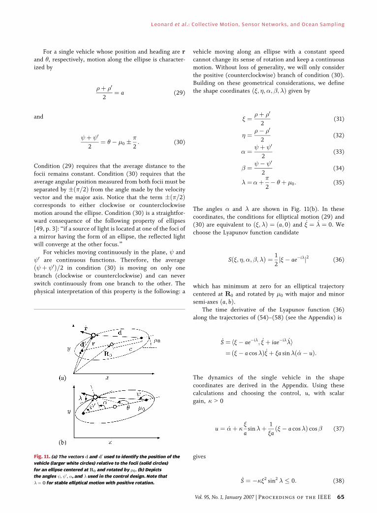
For a single vehicle whose position and heading are rand �, respectively, motion along the ellipse is character-

ized by

þ 0

2¼ a (29)

and

þ 0

2¼ �� 0 �

2: (30)

Condition (29) requires that the average distance to the

focii remains constant. Condition (30) requires that theaverage angular position measured from both focii must be

separated by �ð =2Þ from the angle made by the velocity

vector and the major axis. Notice that the term �ð =2Þcorresponds to either clockwise or counterclockwise

motion around the ellipse. Condition (30) is a straightfor-

ward consequence of the following property of ellipses

[49, p. 3]: Bif a source of light is located at one of the foci of

a mirror having the form of an ellipse, the reflected lightwill converge at the other focus.[

For vehicles moving continuously in the plane, and

0 are continuous functions. Therefore, the average

ð þ 0Þ=2 in condition (30) is moving on only one

branch (clockwise or counterclockwise) and can never

switch continuously from one branch to the other. The

physical interpretation of this property is the following: a

vehicle moving along an ellipse with a constant speedcannot change its sense of rotation and keep a continuous

motion. Without loss of generality, we will only consider

the positive (counterclockwise) branch of condition (30).

Building on these geometrical considerations, we define

the shape coordinates ð�; �; �; �; �Þ given by

� ¼ þ 0

2(31)

� ¼ � 0

2(32)

� ¼ þ 0

2(33)

� ¼ � 0

2(34)

� ¼�þ

2� �þ �0: (35)

The angles � and � are shown in Fig. 11(b). In these

coordinates, the conditions for elliptical motion (29) and(30) are equivalent to ð�; �Þ ¼ ða; 0Þ and _� ¼ _� ¼ 0. We

choose the Lyapunov function candidate

Sð�; �; �; �; �Þ ¼ 1

2j� � ae�i�j2 (36)

which has minimum at zero for an elliptical trajectory

centered at R0 and rotated by �0 with major and minor

semi-axes ða; bÞ.The time derivative of the Lyapunov function (36)

along the trajectories of (54)–(58) (see the Appendix) is

_S ¼h� � ae�i�; _� þ iae�i� _�i¼ ð� � a cos�Þ _� þ �a sin�ð _�� uÞ:

The dynamics of the single vehicle in the shape

coordinates are derived in the Appendix. Using thesecalculations and choosing the control, u, with scalar

gain, � 9 0

u ¼ _�þ ��

asin�þ 1

�að� � a cos�Þ cos� (37)

gives

_S ¼ ��2 sin2 � � 0: (38)

Fig. 11. (a) The vectors d and d0 used to identify the position of the

vehicle (larger white circles) relative to the focii (solid circles)

for an ellipse centered at R0 and rotated by �0. (b) Depicts

the angles , 0, �, and � used in the control design. Note that

� ¼ 0 for stable elliptical motion with positive rotation.



Note that for the circular case a ¼ b ¼ j!oj�1, the control

reduces to the circular control law (16), which, in the

shape coordinates ð; �Þ is given by

u ¼ !0ð1 þ � sin�Þ:

We obtain the following result:

Theorem 6.3: Almost all trajectories of (12) for a single

vehicle subject to the control (37) converge to an elliptical

trajectory centered at R0 and rotated by �0. The size ofthe ellipse is parameterized by the length of its semi-major

and -minor axes, a and b.

Proof: By the Lasalle invariance principle, all

trajectories converge to the largest invariant set for which_S ¼ 0. Using (38), the invariance condition becomes

sin� ¼ 0 since � 9 0. Subject to this condition, the

dynamics of the shape variables ð�; �Þ from (54) and

(58) in the Appendix become

_� ¼ 0 (39)

_� ¼ � 1

�að� � a cos�Þ cos �: (40)

Setting (39) and (40) equal to zero, we obtain the solutions

ð�; �Þ ¼ ða; 0Þ and sin� ¼ cos � ¼ 0. The latter corre-

sponds to trajectories on the major axis of the ellipse

(between the focii) and does not constitute an invariant

set due to the singularities in (37) at the focii. As a result,

all trajectories which do not originate at a focus of the

ellipse asymptotically converge to the set for which

ð�; �Þ ¼ ða; 0Þ. This set corresponds to elliptical motionwith parameters ða; bÞ. h

We briefly discuss how to extend this result to

coordinate groups of vehicles on (separate) ellipses by

coupling their headings as in Section VI-B. Let

R10; . . . ;R

N0 and �1

0; . . . ; �N0 be the location and orienta-

tion of N ellipses with parameters ðak; bkÞ. Also, let uellk be

the ellipse control (37) corresponding to the kth particle.

We assume that the ellipses’ circumferences are all thesame. Then, in order to stabilize each vehicle to its ellipse

and to synchronize the phases of all the vehicles, we

propose the control

uk ¼ uellk þ K

@U1

@�k; k ¼ 1; . . . ;N (41)

for K 9 0, where U1 is the potential function (14). The

convergence analysis of this control law is not pursued in

the present paper but simulations suggest good conver-

gence properties. In Section VII, we compute the optimal

sampling ellipses for a group of two gliders. The optimal

ellipses have the same circumferences and the controllerderived here is applied to this case (see Fig. 16).

VII. OPTIMAL COORDINATEDSOLUTIONS

In this section, we use the sampling metric defined by (8)

to compute near-optimal vehicle trajectories constrained

to ellipses. The objective of this section is to determine theoptimal ellipse parameters as a function of the size, shape,

and characteristic scales of the region of interest and the

capabilities of the sensor platforms. We start by introduc-

ing a convenient formalization of the adaptive sampling

problem using nondimensional numbers. Next, we present

the results of numerical optimization experiments for a

single vehicle on an elliptical trajectory and for a pair of

vehicles on separate ellipses. Lastly, we consider the in-fluence of a uniform flow field on the sampling per-

formance of the ellipse feedback control from the previous

section. We anticipate that the insights from these

numerical results will extend to larger groups of vehicles.

A. Sampling NumbersWe consider a rectangular domain B of size A ¼ BaBb

in which we would like optimal sensor coverage during afinite duration of time T . Ba and Bb are the width and

height of the rectangular domain. The trajectories of the Nvehicles, given by rkðtÞ, and the sampling metric, �ð~rÞ[see (8)], determine the locations and effectiveness of the

sensor measurements. The optimal trajectories, r"kðtÞ, and

the value of the metric at the optimum, �" ¼� �ð~r"Þ, are

obtained by minimizing the metric � among all acceptable

sets of curves, rk, k ¼ 1; . . . ;N, satisfying the constantvelocity constraint in (11).

We decrease the number of dimensions of the

optimization problem by applying the Buckingham -

theorem [51] to reduce the number of variables. Let AvfXgrepresent the space-time average of a quantity X over the

domain B � ½0; T �. Then the initial uncertainty on the

field, �0, is given by

�0 ¼ Av Bðr; t; r; tÞf g: (42)

Recall from Section V-A, the measurement noise is

denoted by n. We now define precisely the correlation

length and the correlation time by

� ¼� 1

Av

ZR2

dr0Bðr; t; r0; tÞBðr; t; r; tÞ

8<:

9=; (43)

� ¼� 1ffiffiffi

p Av

Zþ1�1

dt0Bðr; t; r; t0ÞBðr; t; r; tÞ

8<:

9=;: (44)



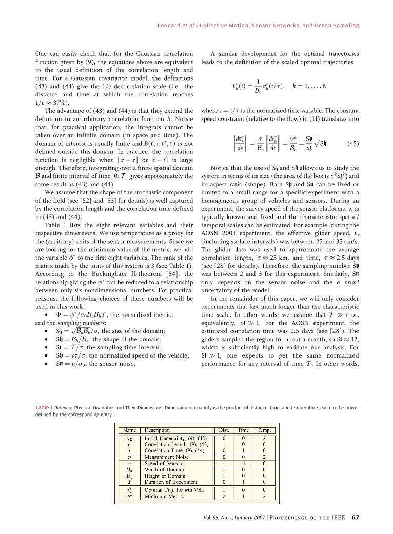
One can easily check that, for the Gaussian correlationfunction given by (9), the equations above are equivalent

to the usual definition of the correlation length and

time. For a Gaussian covariance model, the definitions

(43) and (44) give the 1=e decorrelation scale (i.e., the

distance and time at which the correlation reaches

1=e $ 37%).

The advantage of (43) and (44) is that they extend the

definition to an arbitrary correlation function B. Noticethat, for practical application, the integrals cannot be

taken over an infinite domain (in space and time). The

domain of interest is usually finite and Bðr; t; r0; t0Þ is not

defined outside this domain. In practice, the correlation

function is negligible when kr� rk or jt � t0j is large

enough. Therefore, integrating over a finite spatial domain

B and finite interval of time ½0; T � gives approximately the

same result as (43) and (44).We assume that the shape of the stochastic component

of the field (see [52] and [53] for details) is well captured

by the correlation length and the correlation time defined

in (43) and (44).

Table 1 lists the eight relevant variables and their

respective dimensions. We use temperature as a proxy for

the (arbitrary) units of the sensor measurements. Since we

are looking for the minimum value of the metric, we addthe variable �" to the first eight variables. The rank of the

matrix made by the units of this system is 3 (see Table 1).

According to the Buckingham -theorem [54], the

relationship giving the �" can be reduced to a relationship

between only six nondimensional numbers. For practical

reasons, the following choices of these numbers will be

used in this work:

• � ¼ �"=�0BaBbT , the normalized metric;and the sampling numbers:

• Sz ¼ffiffiffiffiffiffiffiffiffiffiBaBb

p=�, the size of the domain;

• Sh ¼ Bb=Ba, the shape of the domain;

• St ¼ T =� , the sampling time interval;

• Sp ¼ v�=�, the normalized speed of the vehicle;

• Sn ¼ n=�0, the sensor noise.

A similar development for the optimal trajectoriesleads to the definition of the scaled optimal trajectories

r"kðtÞ ¼1

Bar"kðt=�Þ; k ¼ 1; . . . ;N

where s ¼ t=� is the normalized time variable. The constant

speed constraint (relative to the flow) in (11) translates into

dr"kds

�� ¼ �

Ba

dr"kdt

�� ¼ v�

Ba¼ Sp

Sz

ffiffiffiffiffiSh

p: (45)

Notice that the use of Sz and Sh allows us to study the

system in terms of its size (the area of the box is �2Sz2) and

its aspect ratio (shape). Both Sp and Sn can be fixed or

limited to a small range for a specific experiment with a

homogeneous group of vehicles and sensors. During an

experiment, the survey speed of the sensor platforms, v, is

typically known and fixed and the characteristic spatial/

temporal scales can be estimated. For example, during theAOSN 2003 experiment, the effective glider speed, v,

(including surface intervals) was between 25 and 35 cm/s.

The glider data was used to approximate the average

correlation length, � $ 25 km, and time, � $ 2:5 days

(see [28] for details). Therefore, the sampling number Spwas between 2 and 3 for this experiment. Similarly, Snonly depends on the sensor noise and the a prioriuncertainty of the model.

In the remainder of this paper, we will only consider

experiments that last much longer than the characteristic

time scale. In other words, we assume that T % � or,

equivalently, St% 1. For the AOSN experiment, the

estimated correlation time was 2.5 days (see [28]). The

gliders sampled the region for about a month, so St $ 12,

which is sufficiently high to validate our analysis. For

St% 1, one expects to get the same normalizedperformance for any interval of time T . In other words,

Table 1 Relevant Physical Quantities and Their Dimensions. Dimension of quantity is the product of distance, time, and temperature, each to the power

defined by the corresponding entry.



we assume that the metric per unit of area and time, �, isindependent of the sampling time, St. We summarize the

functional dependence of the normalized performance

metric on the four remaining sampling numbers by

� ¼ �ðSz; Sh; Sp; SnÞ: (46)

In the next subsection, we compute the near-optimal

trajectories of a single vehicle among a family of ellipses.

These racetracks can be precomputed or, alternatively,optimized in real-time to maximize the steady-state

performance of the array. The feedback control presented

in Section VI is essential to maintain the vehicles on these

optimal tracks in the presence of strong currents and

limited communication.

B. Optimal Ellipses in Rectangular DomainsIn this subsection, we present optimization results for a

single vehicle following a parameterized elliptical trajec-

tory in a rectangular domain. The objective is to find the

set of parameters yielding the smallest value of the metric,

(46), as a function of the sampling numbers. A system with

only one sensor moving on an elliptical path has six

degrees of freedom: the position and orientation of the

ellipse, the lengths of the semi-major and -minor axes aand b, and the initial phase, �ð0Þ. One can easily checkthat these six parameters determine a unique trajectory for

the vehicle (up to the sense of rotation).

Inspection of (8) directly reveals that the center of the

optimal ellipse necessarily coincides with the middle of

the box B. Moreover, the angle �ð0Þ has no influence on

the metric for St% 1 and can be ignored. In addition, we

assume that the ellipse orientation �0 is parallel to the

long side of the box.For given size Sz, shape Sh, sensor noise Sn, and relative

vehicle speed Sp, the problem reduces to a 2-D space

where the variables are the lengths of the semi-major and -

minor axes of the ellipse, a and b. For example, Fig. 12

shows the contour levels of the metric, i.e., the error map,

as a function of a and b for the sampling numbers Sz ¼ 2,

Sh ¼ 1, Sn ¼ 0:1, and Sp ¼ 3. There is a unique minimum

for a vehicle moving on a circle of radius a ¼ b ¼ 0:256.The fact that the optimal ellipse is a circle is consistent

with the square shape of the domain.

Also notice that the minimum in Fig. 12 is relatively

Bflat.[ Small deviations from a prescribed optimal plan do

not have much influence on the metric; this suggests

robustness to disturbances such as strong currents and

intermittent feedback. For more vehicles, the large phase

space has many local minima. A flat minimum is morerobust and, in practice, is a better solution than a sharp

global minimum. The error map associated with this

optimal trajectory is shown in the upper left panel of

Fig. 13. Next, we investigate the influence of each

sampling number on the optimal elliptical solution.

1) Independence of the Shape Sh: In Fig. 14, we plot theperformance of optimal elliptical trajectories for a single

vehicle within the rectangular box B as a function of the

sampling numbers Sz and Sh. The shape of the optimal

trajectory varies with the shape of the domain; however,

the contour levels of � in the ðSz; ShÞ-plane reveal that �does not depend on Sh. As a result, the same performance

can be achieved on rectangles with different aspect ratio

but with the same area. In particular, if a complex domainsuch as Monterey Bay is divided into several subregions

patrolled by groups of gliders, the shape of the subregions

can be chosen freely. This permits a greater flexibility in

designing sampling plans.

2) Role of Speed Sp and Noise Sn: To study the influence

of the sampling numbers Sp, Sn and Sz on the optimal

trajectories, the optimal ellipses, and the minimum valueof the metric are computed for several values of the

sampling numbers. For example, see Fig. 13 for typical

error maps. We have already determined that the shape Shand the time number St do not influence the solutions so

we present results for Sh ¼ 1 and St% 1. Fig. 15 gives the

optimal nondimensionalized radius ða ¼ bÞ and the

minimum value of the metric, �, as a function of Sz.Each curve corresponds to different values of Sn and Sp.Notice that, for Sz 9 Sp, � becomes independent of Sn.

Fig. 15 also shows that Sp has no influence on the

performance metric (although it does determine the

perimeter of the optimal trajectory). The minimum value

of � is determined entirely by the noise Sn and the size of

the domain Sz. On the other hand, the optimal trajectory

Fig. 12. Nondimensional metric � for one vehicle on an elliptical

trajectory with semi-major and -minor axis lengths a and b. The

gray scale is proportional to the value of �, from low uncertainty

(dark) to high (light). The sampling numbers are Sz ¼ 2, Sh ¼ 1,

Sn ¼ 0:1, and Sp ¼ 3. The minimum gives the optimal ellipse

(a circle) a ¼ b ¼ 0:256.



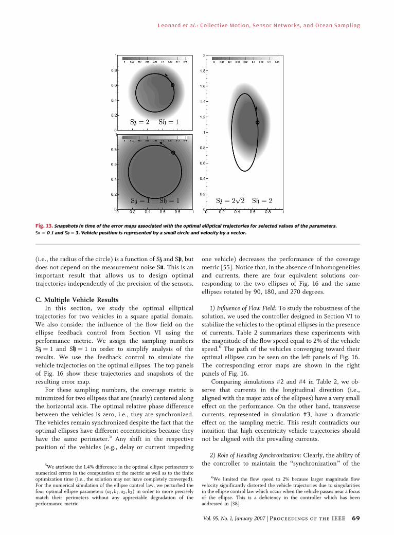
(i.e., the radius of the circle) is a function of Sz and Sp, but

does not depend on the measurement noise Sn. This is an

important result that allows us to design optimaltrajectories independently of the precision of the sensors.

C. Multiple Vehicle ResultsIn this section, we study the optimal elliptical

trajectories for two vehicles in a square spatial domain.

We also consider the influence of the flow field on the

ellipse feedback control from Section VI using the

performance metric. We assign the sampling numbersSz ¼ 1 and Sh ¼ 1 in order to simplify analysis of the

results. We use the feedback control to simulate the

vehicle trajectories on the optimal ellipses. The top panels

of Fig. 16 show these trajectories and snapshots of the

resulting error map.

For these sampling numbers, the coverage metric is

minimized for two ellipses that are (nearly) centered along

the horizontal axis. The optimal relative phase differencebetween the vehicles is zero, i.e., they are synchronized.

The vehicles remain synchronized despite the fact that the

optimal ellipses have different eccentricities because they

have the same perimeter.5 Any shift in the respective

position of the vehicles (e.g., delay or current impeding

one vehicle) decreases the performance of the coverage

metric [55]. Notice that, in the absence of inhomogeneities

and currents, there are four equivalent solutions cor-responding to the two ellipses of Fig. 16 and the same

ellipses rotated by 90, 180, and 270 degrees.

1) Influence of Flow Field: To study the robustness of the

solution, we used the controller designed in Section VI to

stabilize the vehicles to the optimal ellipses in the presence

of currents. Table 2 summarizes these experiments with

the magnitude of the flow speed equal to 2% of the vehiclespeed.6 The path of the vehicles converging toward their

optimal ellipses can be seen on the left panels of Fig. 16.

The corresponding error maps are shown in the right

panels of Fig. 16.

Comparing simulations #2 and #4 in Table 2, we ob-

serve that currents in the longitudinal direction (i.e.,

aligned with the major axis of the ellipses) have a very small

effect on the performance. On the other hand, transversecurrents, represented in simulation #3, have a dramatic

effect on the sampling metric. This result contradicts our

intuition that high eccentricity vehicle trajectories should

not be aligned with the prevailing currents.

2) Role of Heading Synchronization: Clearly, the ability of

the controller to maintain the Bsynchronization[ of the

Fig. 13. Snapshots in time of the error maps associated with the optimal elliptical trajectories for selected values of the parameters.

Sn ¼ 0:1 and Sp ¼ 3. Vehicle position is represented by a small circle and velocity by a vector.

5We attribute the 1.4% difference in the optimal ellipse perimeters tonumerical errors in the computation of the metric as well as to the finiteoptimization time (i.e., the solution may not have completely converged).For the numerical simulation of the ellipse control law, we perturbed thefour optimal ellipse parameters ða1; b1; a2; b2Þ in order to more preciselymatch their perimeters without any appreciable degradation of theperformance metric.

6We limited the flow speed to 2% because larger magnitude flowvelocity significantly distorted the vehicle trajectories due to singularitiesin the ellipse control law which occur when the vehicle passes near a focusof the ellipse. This is a deficiency in the controller which has beenaddressed in [38].



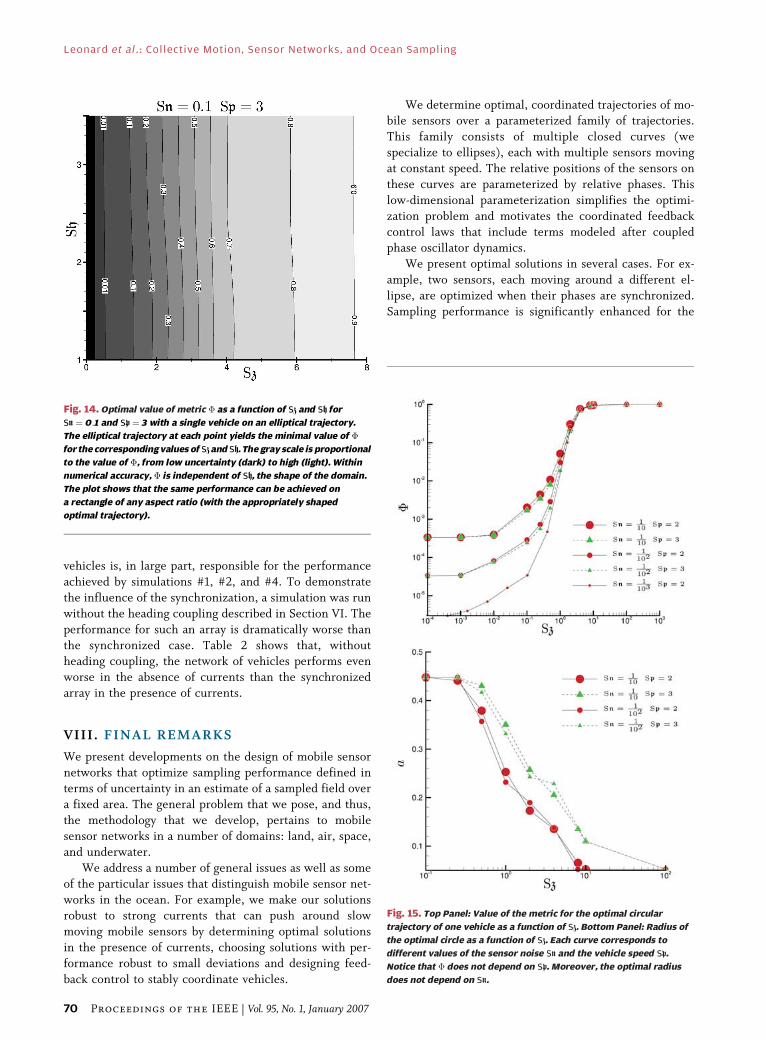
vehicles is, in large part, responsible for the performance

achieved by simulations #1, #2, and #4. To demonstrate

the influence of the synchronization, a simulation was run

without the heading coupling described in Section VI. The

performance for such an array is dramatically worse than

the synchronized case. Table 2 shows that, withoutheading coupling, the network of vehicles performs even

worse in the absence of currents than the synchronized

array in the presence of currents.

VIII. FINAL REMARKS

We present developments on the design of mobile sensor

networks that optimize sampling performance defined interms of uncertainty in an estimate of a sampled field over

a fixed area. The general problem that we pose, and thus,

the methodology that we develop, pertains to mobile

sensor networks in a number of domains: land, air, space,

and underwater.

We address a number of general issues as well as some

of the particular issues that distinguish mobile sensor net-

works in the ocean. For example, we make our solutionsrobust to strong currents that can push around slow

moving mobile sensors by determining optimal solutions

in the presence of currents, choosing solutions with per-

formance robust to small deviations and designing feed-

back control to stably coordinate vehicles.

We determine optimal, coordinated trajectories of mo-bile sensors over a parameterized family of trajectories.

This family consists of multiple closed curves (we

specialize to ellipses), each with multiple sensors moving

at constant speed. The relative positions of the sensors on

these curves are parameterized by relative phases. This

low-dimensional parameterization simplifies the optimi-

zation problem and motivates the coordinated feedback

control laws that include terms modeled after coupledphase oscillator dynamics.

We present optimal solutions in several cases. For ex-

ample, two sensors, each moving around a different el-

lipse, are optimized when their phases are synchronized.

Sampling performance is significantly enhanced for the

Fig. 14. Optimal value of metric � as a function of Sz and Sh for

Sn ¼ 0:1 and Sp ¼ 3 with a single vehicle on an elliptical trajectory.

The elliptical trajectory at each point yields the minimal value of �

for the corresponding values of Sz and Sh. The gray scale is proportional

to the value of �, from low uncertainty (dark) to high (light). Within

numerical accuracy, � is independent of Sh, the shape of the domain.

The plot shows that the same performance can be achieved on

a rectangle of any aspect ratio (with the appropriately shaped

optimal trajectory).

Fig. 15. Top Panel: Value of the metric for the optimal circular

trajectory of one vehicle as a function of Sz. Bottom Panel: Radius of

the optimal circle as a function of Sz. Each curve corresponds to

different values of the sensor noise Sn and the vehicle speed Sp.

Notice that � does not depend on Sp. Moreover, the optimal radius

does not depend on Sn.



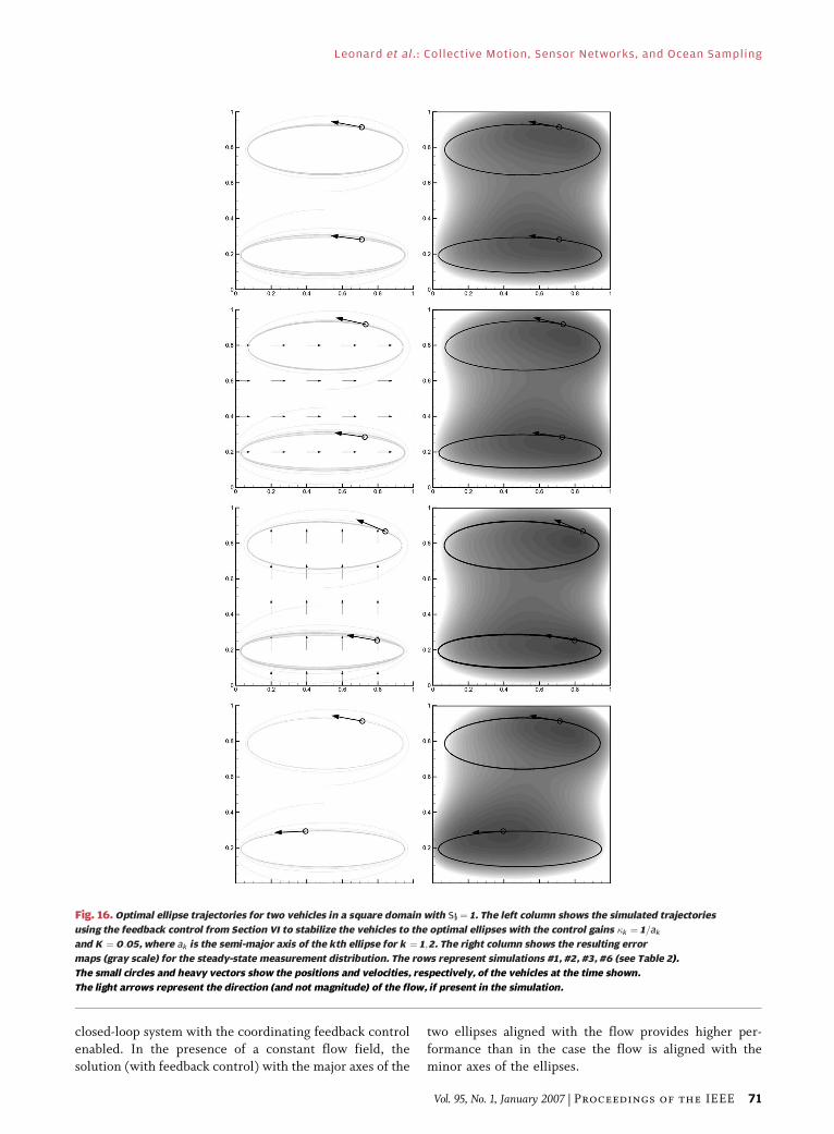
closed-loop system with the coordinating feedback control

enabled. In the presence of a constant flow field, the

solution (with feedback control) with the major axes of the

two ellipses aligned with the flow provides higher per-

formance than in the case the flow is aligned with the

minor axes of the ellipses.

Fig. 16. Optimal ellipse trajectories for two vehicles in a square domain with Sz ¼ 1. The left column shows the simulated trajectories

using the feedback control from Section VI to stabilize the vehicles to the optimal ellipses with the control gains �k ¼ 1=ak

and K ¼ 0:05, where ak is the semi-major axis of the kth ellipse for k ¼ 1;2. The right column shows the resulting error

maps (gray scale) for the steady-state measurement distribution. The rows represent simulations #1, #2, #3, #6 (see Table 2).

The small circles and heavy vectors show the positions and velocities, respectively, of the vehicles at the time shown.

The light arrows represent the direction (and not magnitude) of the flow, if present in the simulation.



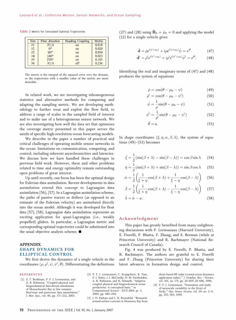
In related work, we are investigating inhomogeneousstatistics and alternative methods for computing and

adapting the sampling metric. We are developing meth-

odology to further treat and exploit the flow field, to

address a range of scales in the sampled field of interest

and to make use of a heterogeneous sensor network. We

are also investigating how well the data set that optimizes

the coverage metric presented in this paper serves the

needs of specific high-resolution ocean forecasting models.We describe in the paper a number of practical and

critical challenges of operating mobile sensor networks in

the ocean: limitations on communication, computing, and

control, including inherent asynchronicities and latencies.

We discuss how we have handled these challenges in

previous field work. However, these and other problems

related to time and energy optimality remain outstanding

open problems of great interest.Up until recently, our focus has been the optimal design

for Eulerian data assimilation. Recent developments in data

assimilation extend this concept to Lagrangian data

assimilation [56], [57]. In a Lagrangian assimilation scheme,

the paths of passive tracers or drifters (as opposed to an

estimate of the Eulerian velocity) are assimilated directly

into the ocean model. Although it was developed for float

data [57], [58], Lagrangian data assimilation represents anexciting application for quasi-Lagrangian (i.e., weakly

propelled) gliders. In particular, a Lagrangian metric and

corresponding optimal trajectories could be substituted into

the usual objective analysis scheme. h

APPENDIX I.SHAPE DYNAMICS FORELLIPTICAL CONTROL

We first derive the dynamics of a single vehicle in the

coordinates ð; 0; ; 0; �Þ. Differentiating the definitions

(27) and (28) using _R0 ¼ _�0 ¼ 0 and applying the model(12) for a single vehicle gives

_d ¼ _eið þ�0Þ þ ieið þ�0Þ _ ¼ ei� (47)

_d0 ¼ _0eið 0þ�0Þ þ i0eið 0þ�0Þ _ 0 ¼ ei�: (48)

Identifying the real and imaginary terms of (47) and (48)

produces the system of equations

_ ¼ cosð�� 0 � Þ (49)

_0 ¼ cosð�� 0 � 0Þ (50)

_ ¼ 1

sinð�� 0 � Þ (51)

_ 0 ¼ 1

0sinð�� 0 � 0Þ (52)

_� ¼ u: (53)

In shape coordinates ð�; �; �; �; �Þ, the system of equa-

tions (49)–(53) becomes

_� ¼ 1

2sinð� þ �Þ � sinð� � �Þð Þ ¼ cos� sin� (54)

_� ¼ 1

2sinð� þ �Þ þ sinð� � �Þð Þ ¼ sin� cos� (55)

_� ¼ 1

2

1

� þ �cosð� þ �Þ þ 1

� � �cosð� � �Þ

� �(56)

_� ¼ 1

2

1

� þ �cosð� þ �Þ � 1

� � �cosð� � �Þ

� �(57)

_� ¼ _�� u: (58)

Acknowledgment

This paper has greatly benefited from many enlighten-

ing discussions with P. Lermusiaux (Harvard University),

E. Fiorelli, P. Bhatta, F. Zhang, and S. Berman (while at

Princeton University) and R. Bachmayer (National Re-

search Council of Canada).

Fig. 4 was produced by E. Fiorelli, P. Bhatta, and

R. Bachmayer. The authors are grateful to E. Fiorelli

and F. Zhang (Princeton University) for sharing theirlatest advances in formation design and control.

REF ERENCE S

[1] S. T. Besiktepe, P. F. J. Lermusiaux, andA. R. Robinson, BCoupled physical andbiogeochemical data-driven simulationsof Massachusetts Bay in late summer:Real-time and postcruise data assimilation,[J. Mar. Syst., vol. 40, pp. 171–212, 2003.

[2] P. F. J. Lermusiaux, C. Evangelinos, R. Tian,P. J. Haley, J. J. McCarthy, N. M. Patrikalakis,A. R. Robinson, and H. Schmidt, BAdaptivecoupled physical and biogeochemical oceanpredictions: A conceptual basis,[ inComputational ScienceVICCS 2004, pt. 3,2004, pp. 685–692.

[3] J. D. Paduan and L. K. Rosenfeld, BRemotelysensed surface currents in Monterey Bay from

shore-based HF radar (coastal ocean dynamicsapplication radar),[ J. Geophys. Res.VOceans,vol. 101, no. C9, pp. 20 669–20 686, 1996.

[4] P. F. J. Lermusiaux, BEstimation and studyof mesoscale variability in the Strait ofSicily,[ Dyn. Atmos. Oceans, vol. 29, no. 2–4,pp. 255–303, 1999.

Table 2 Metric for Simulated Optimal Trajectories

The metric is the integral of the squared error over the domain,so the trajectories with a smaller value of the metric are moredesirable.



[5] C. H. Pilskaln, C. Lehmann, J. B. Paduan, andM. W. Silver, BSpatial and temporal dynamicsin marine aggregate abundance, sinking rateand flux: Monterey Bay, central California,[Deep-Sea Rese. IIVTopical StudiesOceanogr., vol. 45, no. 8–9, pp. 1803–1837,1998.

[6] W. F. Dabberdt and T. W. Schlatter,BResearch opportunities from emergingatmospheric observing and modelingcapabilities,[ Bull. Amer. Meteorol. Soc.,vol. 77, no. 2, pp. 305–323, 1996.

[7] A. C. Lorenc, R. S. Bell, and B. Macpherson,BThe meteorological-office analysis correctiondata assimilation scheme,[ Q. J. R. Meteorol.Soc., vol. 117, no. 497, pp. 59–89, 1991.

[8] C. B. Paris, R. K. Cowen, K. M. M. Lwiza,D. P. Wang, and D. B. Olson, BMultivariateobjective analysis of the coastal circulation ofBarbados, West Indies: Implication for larvaltransport,[ Deep-Sea Res. IVOceanogr. Res.Papers, vol. 49, no. 8, pp. 1363–1386, 2002.

[9] J. Willcox, J. Bellingham, Y. Zhang, andA. Baggeroer, BPerformance metrics foroceanographic surveys with autonomousunderwater vehicles,[ IEEE J. Ocean. Eng.,vol. 26, no. 4, pp. 711–725, Oct. 2001.

[10] A. L. Bertozzi, M. Kemp, and D. Marthaler,BDetermining environmental boundaries:Asynchronous communication andphysical scales,[ in Cooperative Control,A Post-Workshop Volume: 2003 Block IslandWorkshop on Cooperative Control, V. Kumar,N. Leonard, and A. Morse, Eds. New York:Springer-Verlag, 2005, pp. 35–42.

[11] D. Marthaler and A. L. Bertozzi, BTrackingenvironmental level sets with autonomousvehicles,[ in Recent Developments inCooperative Control and Optimization,S. Butenko, R. Murphey, and P. Pardalos,Eds. Norwell, MA: Kluwer, 2003.

[12] F. Zhang and N. E. Leonard, BGeneratingcontour plots using multiple sensorplatforms,[ in Proc. IEEE SwarmIntelligence Symp., 2005.

[13] E. Fiorelli, N. E. Leonard, P. Bhatta,D. Paley, R. Bachmayer, and D. Fratantoni,BMulti-AUV control and adaptive sampling inMonterey Bay,[ in Proc. IEEE AUV 2004:Workshop on Multiple AUV Operations, 2004,and IEEE J. Ocean. Eng., vol. 31, no. 3,July 2006.

[14] A. Eliassen and J. S. Sawyer, BUpper airnetwork requirements for numerical weatherprediction,[ Tech. Note World Meteorol. Org.vol. 29, 1954.

[15] L. S. Gandin, GidrometerologicheskoeIzdatelstvoVObjective Analysis ofMeteorological Fields, Leningrad, Jerusalem(English Translation by Israeli Programfor Scientific Translations), 1963.

[16] F. P. Bretherton, R. E. Davis, andC. B. Fandry, BA technique for objectiveanalysis and design of oceanographicexperiments applied to MODE-73,[Deep-Sea Res., vol. 23, pp. 559–582, 1976.

[17] C. H. Pilskaln, J. B. Paduan, F. P. Chavez,R. Y. Anderson, and W. M. Berelson, BCarbonexport and regeneration in the coastalupwelling system of Monterey Bay,Central California,[ J. Mar. Res., vol. 54, no. 6,pp. 1149–1178, 1996.

[18] T. Hirawake, T. Odate, and M. Fukuchi,BLong-term variation of surfacephytoplankton chlorophylla in thesouthern ocean during 1965–2002,[ Geophys.Res. Lett., vol. 32, no. 5-L05606, 2005.

[19] D. K. Steinberg, M. W. Silver, C. H. Pilskaln,S. L. Coale, and J. B. Paduan, BMidwaterzooplankton communities on pelagic detritus

(giant larvacean houses) in Monterey Bay,California,[ Limnol. Oceanogr., vol. 39, no. 7,pp. 1606–1620, 1994.

[20] J. Bellingham, BNew oceanographic uses ofautonomous underwater vehicles,[ Mar.Technol. Soc. J., vol. 31, no. 3, pp. 34–47, 1997.

[21] T. B. Curtin, J. G. Bellingham, J. Catipovic,and D. Webb, BAutonomous oceanographicsampling networks,[ Oceanography, vol. 6,no. 3, pp. 86–94, 1993.

[22] J. Sherman, R. E. Davis, W. B. Owens, andJ. Valdes, BThe autonomous underwater gliderFSpray_,[ IEEE J. Ocean. Eng., vol. 26, no. 4,pp. 437–446, Oct. 2001.

[23] D. Webb, P. Simonetti, and C. Jones,BSLOCUM: An underwater glider propelledby environmental energy,[ IEEE J. Ocean.Eng., vol. 26, no. 4, pp. 447–452, Oct. 2001.

[24] C. C. Eriksen, T. J. Osse, T. Light, R. D. Wen,T. W. Lehmann, P. L. Sabin, J. W. Ballard, andA. M. Chiodi, BSeaglider: A long rangeautonomous underwater vehicle foroceanographic research,[ IEEE J. Ocean. Eng.,vol. 26, no. 4, pp. 424–436, Oct. 2001.

[25] D. Steere, A. Baptista, D. McNamee,C. Pu, and J. Walpole, BResearch challengesin environmental observation andforecasting systems,[ in Proc. 6th Int.Conf. Mobile Computing and Networking(MOBICOMM), 2000.

[26] R. Cardell-Oliver, K. Smettem, M. Krantz,and K. Meyer, BField testing a wirelesssensor network for reactive environmentalmonitoring,[ in Proc. Int. Conf. IntelligentSensors, Sensor Networks and InformationProcessing ISSNIP-04, 2004.

[27] MBARI. (2003). Autonomous OceanSampling Network. [Online]. Available:http://www.mbari.org/aosn.

[28] D. L. Rudnick, R. E. Davis, C. C. Eriksen,D. M. Fratantoni, and M. J. Perry,BUnderwater gliders for ocean research,[Mar. Technol. Soc. J., vol. 38, no. 1, pp. 48–59,2004.

[29] P. Ogren, E. Fiorelli, and N. E. Leonard,BCooperative control of mobile sensornetworks: Adaptive gradient climbing in adistributed environment,[ IEEE Trans. Autom.Control, vol. 49, no. 8, pp. 1292–1302,Aug. 2004.

[30] E. Fiorelli, P. Bhatta, N. E. Leonard, andI. Shulman, BAdaptive sampling usingfeedback control of an autonomousunderwater glider fleet,[ in Proc. Symp.Unmanned Untethered SubmersibleTechnology, 2003.

[31] J. Graver, BUnderwater gliders: Dynamics,control and design,[ Ph.D. dissertation,Princeton Univ., Princeton, NJ, 2005.

[32] P. F. J. Lermusiaux and A. R. Robinson, BDataassimilation via error subspace statisticalestimation. Part I: Theory and schemes,[Monthly Weather Rev., vol. 127, no. 7,pp. 1385–1407, 1999.

[33] P. E. Lermusiaux, BData assimilation via errorsubspace statistical estimation. Part II: MiddleAtlantic Bight shelfbreak front simulationsand ESSE validation,[ Monthly Weather Rev.,vol. 127, no. 7, pp. 1408–1432, 1999.

[34] I. Shulman, C. R. Wu, J. K. Lewis,J. D. Paduan, L. K. Rosenfeld, J. C. Kindle,S. R. Ramp, and C. A. Collins, BHighresolution modeling and data assimilationin the Monterey Bay area,[ Cont. Shelf Res.,vol. 22, no. 8, pp. 1129–1151, 2002.

[35] P. F. J. Lermusiaux, BUncertainty estimationand prediction for the interdisciplinaryocean,[ J. Comput. Phys., 2005.

[36] I. Shulman, D. J. McGillicuddy, M. A. Moline,S. H. D. Haddock, J. Kindle, D. Nechaev, andM. W. Phelps, BBiolumineseence intensitymodeling and sampling strategyoptimization,[ J. Atmos. Ocean. Technol.,vol. 22, pp. 1267–1281, 2005.

[37] S. R. Ramp, J. D. Paduan, I. Shulman,J. Kindle, F. L. Bahr, and F. Chavez,BObservations of upwelling and relaxationevents in the Northern Monterey Bay duringAugust 2000,[ J. Geophys. Res.VOceans,vol. 110, no. C07013, 2005.

[38] D. Paley, N. E. Leonard, and R. Sepulchre,BCollective motion of self-propelled particles:Stabilizing symmetric formations on closedcurves,[ in Proc. 44th IEEE Conf. Decision andControl, 2006.

[39] T. Inanc, S. Shadden, and J. Marsden,BOptimal trajectory generation in oceanflows,[ in Proc. 43rd IEEE Conf. Decisionand Control, 2004.

[40] S. Berman, BDevelopment of thermoclinetracking capabilities for the Slocumunderwater glider,[ Princeton Univ.,Princeton, NJ, 2004, Tech. Rep.

[41] P. F. J. Lermusiaux, D. G. M. Anderson, andC. J. Lozano, BOn the mapping of multivariategeophysical fields: Error and variabilitysubspace estimates,[ Q. J. R. Meteorol. Soc.,vol. 126, no. 565, pp. 1387–1429, 2000.

[42] P. F. J. Lermusiaux, BOn the mapping ofmultivariate geophysical fields: Sensitivities tosize, scales, and dynamcs,[ J. Atmos. Ocean.Technol., vol. 19, no. 10, pp. 1602–1637, 2002.

[43] A. Bennett, Inverse Modeling of the Ocean andAtmosphere. Cambridge, U.K.: CambridgeUniv. Press, 2002.

[44] E. Kalnay, Atmospheric Modeling, DataAssimilation, and Predictability. Cambridge,U.K.: Cambridge Univ. Press, 2003.

[45] B. Grocholsky. (2002). BInformation-theoretic control of multiple sensorplatforms,[ Ph.D. dissertation, Univ. Sydney,Sydney, Australia. [Online]. Available: http://www.acfr.usyd.edu.au.

[46] A. S. Bower, D. M. Fratantoni, W. E. Johns,and H. Peters, BGulf of Aden eddies and theirimpact on Red Sea water,[ Geophys. Res. Lett.,vol. 29, p. 21-1, Nov. 2002.

[47] R. Sepulchre, D. Paley, and N. E. Leonard,BCollective motion in the plane: All-to-allcommunication,[ IEEE Trans. Autom.Control, to be published.

[48] D. Paley, N. E. Leonard, and R. Sepulchre,BOscillator models and collective motion:Splay state stabilization of self-propelledparticles,[ in Proc. 44th IEEE Conf. Decisionand Control, 2005.

[49] D. Paley, N. Leonard, and R. Sepulchre,BCollective motion: Bistability and trajectorytracking,[ in Proc. 43rd IEEE Conf. Decisionand Control, 2004.

[50] D. Hilbert and S. Cohn-Vossen, Geometry andthe Imagination, 2nd ed. Chelsea: Chelsea,1999.

[51] E. Buckingham, BOn physically similarsystems; illustrations of the use ofdimensional equations,[ Phys. Rev., vol. 4,pp. 345–376, 1914.

[52] H. J. Thiebaux, BExperiment with correlationrepresentations for objective analysis,[Monthly Weather Rev., vol. 103, pp. 617–627,1975.

[53] VV, BAnisotropic correlation functions forobjective analysis,[ Monthly Weather Rev.,vol. 104, pp. 994–1002, 1976.

[54] W. Curtis, J. Logan, and W. Parker,BDimensional analysis and the theorem,[



Linear Algebra Appl., vol. 47, pp. 117–126,1982.

[55] S. Berman, BEstimation of ocean fielddecorrelation scales for the design ofunderwater glider sampling trajectories,[undergraduate senior thesis, Princeton Univ.,Princeton, NJ, 2005.

[56] K. Ide, L. Kuznetsov, and C. K. R. T. Jones,BLagrangian data assimilation for point vortexsystems,[ J. Turbulence, vol. 3, no. 053, 2002.

[57] A. Molcard, A. Griffa, and T. M. Ozgokmen,BLagrangian data assimilation in multilayerprimitive equation ocean models,[ J. Atmos.Ocean. Technol., vol. 22, no. 1, pp. 70–83,2005.

[58] A. Molcard, L. I. Piterbarg, A. Griffa,T. M. Ozgokmen, and A. J. Mariano,BAssimilation of drifter observations forthe reconstruction of the Euleriancirculation field,[ J. Geophys. Res.VOceans,vol. 108, no. C3, 2003, Art. No. 3056.

ABOUT THE AUT HORS

Naomi Ehrich Leonard (Fellow, IEEE) received

the B.S.E. degree in mechanical engineering from

Princeton University, Princeton, NJ, in 1985 and

the M.S. and Ph.D. degrees in electrical engineer-

ing from the University of Maryland, College Park,

in 1991 and 1994, respectively.

From 1985 to 1989, she worked as an Engineer

in the electric power industry for MPR Associates,

Inc. She is now Professor of Mechanical and

Aerospace Engineering and an associated faculty

member of the Program in Applied and Computational Mathematics at

Princeton University. Her current research interests include nonlinear

control and dynamics, cooperative control, mobile sensor networks,

autonomous underwater vehicles, adaptive ocean sampling, and collec-

tive motion in fish schools.

Derek A. Paley (Student Member, IEEE) received

the B.S. degree in applied physics from Yale

University, New Haven, CT, in 1997. He is working

toward the Ph.D. degree in the Dynamical Control

Systems Laboratory, Mechanical and Aerospace

Engineering Department, Princeton University,

Princeton, NJ.

From 1997 to 2000, he was an Analyst at

Metron Inc., a scientific consulting firm in Reston,

VA. From 2000 to 2002, he was a Software

Engineer at Bluefin Robotics Corp., Cambridge, MA. His research interests

are in dynamics and control, specifically cooperative control and

collective motion with application to designing mobile sensor networks

and modeling animal aggregations.

Francois Lekien graduated from the Ecole

Polytechnique of the Universite Libre de Brux-

elles in 1999 and received the Ph.D. degree in

control and dynamical systems from the Califor-

nia Institute of Technology in 2003.

During 2003, he was a postdoctoral scholar in

mechanical engineering at the Massachusetts

Institute of Technology. His investigations focus

on nonlinear dynamics in turbulent flows, coher-

ent structures, and modal reconstruction of

coastal currents. He is now a Research Associate at Princeton University,

Princeton, NJ.

Rodolphe Sepulchre (Member, IEEE) received the

engineering degree and Ph.D. degree in applied

mathematics from the University of Louvain,

Louvain, Belgium, in 1990 and 1994, respectively.

From 1994 to 1996, he held a postdoctoral

position at the University of California, Santa

Barbara. In 2002–2003, he held a visiting position

at Princeton University, Princeton, NJ. He is now a

Professor in the Department of Electrical Engi-

neering and Computer Science at the University of

Liege, Belgium. His research focuses on theory and applications of

nonlinear dynamical systems. He is co-author with M. Jankovic and

P. Kokotovic of the book Constructive Nonlinear Control (Springer-

Verlag, 1997). He serves as an Associate Editor for the journal

Mathematics of Control, Signals, and Systems.

David M. Fratantoni (Member, IEEE) received the

B.S. degree in ocean engineering from Virginia

Tech, Blacksburg, VA, in 1990 and the Ph.D. degree

in physical oceanography from the University of

Miami, Miami, FL, in 1996.

He completed a postdoctoral fellowship at the

Woods Hole Oceanographic Institution, Woods,

Hole, MA, and was appointed to the scientific staff

in 1998. Recent research topics include observa-

tional studies of ocean circulation with an empha-

sis on mesoscale processes; investigation of the structure and

significance of rings, eddies, and fronts; exploration of the relationships

between physics and biology on various scales; and development of

instrument platforms, sensors, and observing networks.

Russ E. Davis received the B.S. degree from

University of California at Berkeley in 1963 and the

Ph.D. degree from Stanford University, Stanford,

CA, in 1967, both in chemical engineering.

He joined the faculty of the Scripps Institution

of Oceanography, University of California at San

Diego, La Jolla, in 1969, where he has worked on

surface wave generation by wind, mixed layer

dynamics, mid-ocean mesoscale eddies and, dur-

ing the World Ocean Circulation Experiment,

basin-scale intermediate depth flows. A number of observational

instruments were developed to further these studies including the

Vector Measuring Current Meter, the shipboard Acoustic Doppler Current

Profiler, the CODE surface drifter, self-contained ADCPs for moorings, the

autonomous profiling float, and the BSpray[ variant of buoyancy driven

underwater gliders.



Documents

INVITED PAPER Collective Motion, Sensor …naomi/publications/2007/...INVITED PAPER Collective Motion, Sensor Networks, and Ocean Sampling The goal is design and control of optimum