Ion Optics Through the Eyes of SIMION 6simion.com/docs/class-handout.pdf · · 2009-11-24Ion Optics Through the Eyes of SIMION 6.0 AN ASMS SHORT COURSE ... Run EINZEL Demo Clear

Ion Optics Through the Eyes of SIMION 6.0

AN ASMS SHORT COURSE

Portland ASMS Conference

May 11-12, 1996

Instructors

David A. Dahland

Anthony D. Appelhans

Course Outline

Course Outline - Page 1

Topics - May 11 am How ManualGet Class Organized Introduce Instructors

State Objectives of CourseExplain How Course will be ConductedDivide Class into Working Groups

Session 1

Learn GUI/SIMION Usage

Discuss SIMION and GUI philosophy (guided tour)Basic GUI

Objects and HelpFile ManagerOther GUI Options (Color, Sounds, and etc.)

Viewing Basics (using EXTRACT.PA)Change View Orientation and Quality2D Zoom and Scrolling3D Zoom

Run EINZEL DemoClear Memory and Load with ViewLoad and Fly Ions (alone or grouped) Potential Energy Surfaces and ContouringReRun, Single Step, Fast Adjust with Ions FlyingFly Ions with Charge Repulsion ActivePrinting Views and Screens

1-1F-1F-6

F-12F-2

7-107-127-13C-2

2-12,7-88-4

7-19,7-348-12,7-28

8-15G-1,G-5

Session 2

Introduce Ion Optics Concepts

Discuss Radius of RefractionDiscuss Ion Definitions

Defining Ions in Groups (.FLY)Defining Ions Individually (.ION)Defining Ions Outside of SIMION (.ION)

Discuss Data Recording (.REC)Controlling Data Recording to a FileWhat, When, How, and to WhereUsing the Data Monitoring ScreenUser Programs can Record Data Too!

Class Lab:Run electrostatic and magnetic refraction demosCompare changes in ion massCompare changes in ion KECompare changes in field potentials

2-48-48-48-8

8-10,D-48-178-17

8-20/258-25I-11

Coffee Break Get it while you can - during lab

Session 3

Creating and Refining 2D PotentialArrays

Discuss Potential Arrays and Refining MethodsDiscuss How Potentials are Changed

Fast AdjustFast Scaling

Discuss How Magnetic Arrays are Defined and theEffect of the ng parameter

Introduce the Notion of Geometry Files

Class Lab:Create Fast Adjust Electrostatic LensRefine Fast Adjust ArrayFly Ions and Fast adjust VoltagesCreate and Refine Fast Scaling Magnetic LensFly Ions through Magnetic LensUse New Function with Canned Geometry File

2-6,6-14-1,5-1

2-11,6-12-112-102-10J-1

Lunch

Course Outline


Topics - May 11 pm How ManualSession 4

Time-of-Flight Principles

Discuss Use of Instances in WorkbenchImpact of Trajectory Computational Quality

Discuss Time-of-Flight Concepts

Class Lab:Run Linear TOF Demo - with ion bunchingChange Computational Quality on Linear TOFRun Reflectron TOF DemoDetermine drift time/reflectron time ratiosEdit Ions and TOF Instances to change ratioExamine impact of refraction on time focusing

7-1,7-38-13

Session 5

FTMS ICR Cell Principles

Discuss the Use of User Programs in ICR Cell DemoThe Concept of Adjustable Variables

Discuss ICR Cell Concepts

Class Lab:Run ICR Cell DemoView Single Ion TrajectoriesPump Kinetic Energy into the IonsView Groups of Ions and Separation by MassMeasure The Cyclotron Frequency with SIMIONTrap Ions Formed Outside the ICR Cell

I-1I-14


Session 6

Quadrupole Principles

Discuss Use of Instances and User Programs in DemoDiscuss Quadrupole Concepts

Quadrupole Entrance and Exit Region Issues

Class Lab:Run Quadrupole DemoExamine Trajectory Patterns of Random IonsFind the Three Instance Used for DemoExamine how the Potential arrays are DefinedExperiment with Mass Filtering in the QuadrupoleExplore How to get Ions Into the Quadrupole

7-3,I-1

Session 7

Ion Trap Principles

Discuss Ion Trap ConceptsImpact of Cooling GasDiscuss Use of End-Cap TickleExternal Introduction of Ions

Class Lab:Run Ion Trap Demo on Single IonFly Ions Using Damping and Charge RepulsionTickle Ions with End CapsInject External Ions Into the TrapModel MSMS Fragmentation in the Trap

Course Outline


Topics - May 12 am How ManualSession 8

Creating 3D Arrays With Modify

Discuss Modify with 3D Arrays2D to 3D and 3D to 2D Conversions3D Layers and Marking in ModifyFind OptionsReplace, Edge, Move, Copy, and etc.

Discuss the Double and Halve Functions

Class Lab:Use Double and Halve and Inspect the Jags

5-75-9

5-10,5-145-205-215-4

Session 9

Creating Arrays with GeometryFiles

Discuss Pros and Cons of Geometry FilesNested Structure Used in Geometry FilesDiscuss Importance of Locate CommandRecommend for Geometry File Methods

Class Lab:Insert Geometry File in Different Sizes ArraysModify a Geometry FileCreate a Functional Geometry File

J-1J-2,J-4

J-6J-21


Session 10

Introduction to User Programming

Discuss User Programs and How They are UsedUser Program SegmentsLanguage StructureAdjustable, Static, and Reserved Variables

Class Lab:Connect an Existing User Program File to ArrayExplore User Program Development SystemModify a User Program FileAdd a New Program SegmentDevelop Own User Program Code

I-1I-2I-4

I-14

Lunch

Course Outline


Topics - May 12 pm How ManualSession 11

Interest Directed Exploration

Reform into Several Interest Groups (as per studentinterest):

1. Further Ion Optics Simulations:Simple LensesTOFsICR CellsQuadrupolesIon Trapsor whatever

2. More Advanced SIMION Concepts:Advanced Instance TricksCreating a Serious Geometry FileAdvanced User Programmingor some other SIMION topic

3. OR Attacking One or More Problems Suggested bythe Instructors.

Students can form the interest groups they desire andtransfer between them at will.


Interest Directed Exploration Cont. Second segment gives opportunity for creating new groups,transferring between groups, or continued groupexploration as dictated by student interest.

Session 1

Session 1 - Page 1

Session 1 - Learn GUI/SIMION Usage

This Lab’s Files are found in Directory: C:\CLASS\SESSION1

Learn by doing Discussion (SIMION main menu visible):

1. GUI Objects (buttons, panels, iolines, and windows)File Manager(selecting: drive, directory, files, and other options)Class Activity (create a subdirectory, copy files into it, and then delete subdirectory)

2. Other GUI Options (colors, sounds, delays, mouse, and video)Class Activity (Turn off/on clicks, change colors, change mouse sensitivity, change videoresolution)

3. Use Old (load EXTRACT.PA into memory)Enter View (demonstrate view orientations and drawing quality options)Class Activity (Load EXTRACT.PA and change view orientation and drawing quality)

4. Demonstrate 2D Zoom and Scrolling via area markingDemonstrate 2D Zoom and Scrolling via Window button (both page and normal view)Class Activity (Practice 2D Zooming and Scrolling)

5. Introduce 3D Zoom VolumesDemonstrate 3D Zoom via area markingDemonstrate 3D Zoom via the Window Button (page and normal view) and within-view pointingClass Activity (Practice the various forms of 3D Zooming)

6. Remove all .PAs from memoryLoad EINZEL.IOB demo into ViewLoad Ion .FLY file and fly ions (alone, grouped, as lines, and dots)Class Activity (Load EINZEL.IOB, EINZEL.FLY, and fly ions in various ways)

7. Demonstrate Potential Energy SurfacesDemonstrate Contouring (2D and 3D)Class Activity (Exercise PE surface and contouring options)

8. Demonstrate use of Rerun and how to single time-step ionsDemonstrate use of Fast Adjust while Ions are FlyingClass Activity (Exercise Fast Adjust and single time-step options while ions are flying)

9. Discuss/Demonstrate charge repulsion (Factor - beam)Class Activity (Practice using beam repulsion with EINZEL)

10. Discuss how to print (view, objects, or entire screens)Introduce the various printing optionsDiscuss how to use the annotatorClass Activity (Print a selected view and an entire screen)

Session 1

Session 1 - Page 2

This page intentionally left blank

Session 2

Session 2 - Page 1

Session 2 - Ion Optics Concepts

Some Basic Ion Optics Concepts

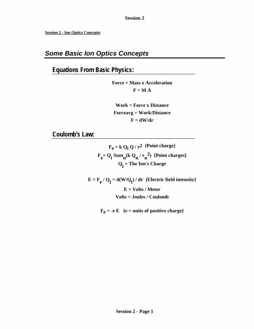
Equations From Basic Physics:

Force = Mass x AccelerationF = M A

Work = Force x DistanceForceavg = Work/Distance

F = dW/dr

Coulomb's Law:

Fe = k Qi Q / r2 {Point charge}

Fe= Qi Sumn(k Qn / rn2) {Point charges}

Qi = The Ion's Charge

E = Fe / Qi = d(W/Qi) / dr {Electric field intensity}

E = Volts / MeterVolts = Joules / Coulomb

Fe = -e E {e = units of positive charge}

Session 2

Session 2 - Page 2

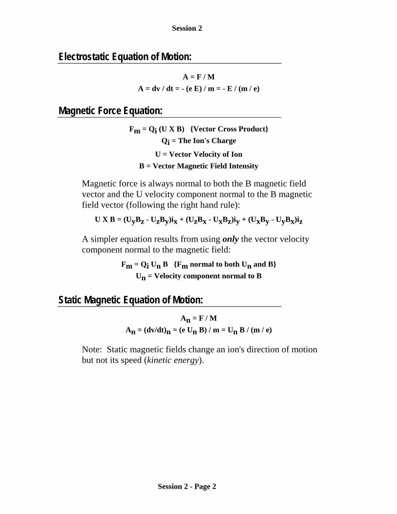
Electrostatic Equation of Motion:

A = F / MA = dv / dt = - (e E) / m = - E / (m / e)

Magnetic Force Equation:Fm = Qi (U X B) {Vector Cross Product}

Qi = The Ion's Charge

U = Vector Velocity of IonB = Vector Magnetic Field Intensity

Magnetic force is always normal to both the B magnetic fieldvector and the U velocity component normal to the B magneticfield vector (following the right hand rule):

U X B = (UyBz - UzBy)ix + (UzBx - UxBz)iy + (UxBy - UyBx)iz

A simpler equation results from using only the vector velocitycomponent normal to the magnetic field:

Fm = Qi Un B {Fm normal to both Un and B}Un = Velocity component normal to B

Static Magnetic Equation of Motion:An = F / M

An = (dv/dt)n = (e Un B) / m = Un B / (m / e)

Note: Static magnetic fields change an ion's direction of motionbut not its speed (kinetic energy).

Session 2

Session 2 - Page 3

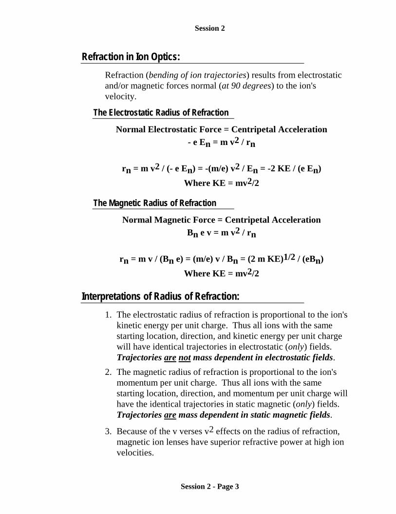
Refraction in Ion Optics:Refraction (bending of ion trajectories) results from electrostaticand/or magnetic forces normal (at 90 degrees) to the ion'svelocity.

The Electrostatic Radius of Refraction

Normal Electrostatic Force = Centripetal Acceleration- e En = m v2 / rn

rn = m v2 / (- e En) = -(m/e) v2 / En = -2 KE / (e En)Where KE = mv2/2

The Magnetic Radius of Refraction

Normal Magnetic Force = Centripetal AccelerationBn e v = m v2 / rn

rn = m v / (Bn e) = (m/e) v / Bn = (2 m KE)1/2 / (eBn)Where KE = mv2/2

Interpretations of Radius of Refraction:1. The electrostatic radius of refraction is proportional to the ion's

kinetic energy per unit charge. Thus all ions with the samestarting location, direction, and kinetic energy per unit chargewill have identical trajectories in electrostatic (only) fields.Trajectories are not mass dependent in electrostatic fields.

2. The magnetic radius of refraction is proportional to the ion'smomentum per unit charge. Thus all ions with the samestarting location, direction, and momentum per unit charge willhave the identical trajectories in static magnetic (only) fields.Trajectories are mass dependent in static magnetic fields.

3. Because of the v verses v2 effects on the radius of refraction,magnetic ion lenses have superior refractive power at high ionvelocities.

Session 2

Session 2 - Page 4

Light Optics Verses Ion Optics

There are significant differences between light and ion optics:

Radius of RefractionLight optics make use of sharp transitions of light velocity (e.g.lens edges) to refract light. These are very sharp and well defined(by lens shape) transitions. The radius of refraction is infiniteeverywhere (straight lines) except at transition boundaries whereit approaches zero (sharp bends).Ion optics makes use of electric field intensity and charged particlemotion in magnetic fields to refract ion trajectories. This is adistributed effect resulting in gradual changes in the radius ofrefraction. Desired electrostatic/magnetic field shapes are muchharder to determine and create since they result from complexinteractions of electrode/pole shapes, spacing, potentials and canbe modified significantly by space charge.

Energy (Chromatic) SpreadsVisible light varies in energy by less than a factor of two.Ions can vary in initial relative energies (or momentum formagnetic) by orders of magnitude. This is why strong initialaccelerations are often applied to ions to reduce the relativeenergy spread.

Physical ModelingLight optics can be modeled using physical optics benches(interior beam shapes can be seen with smoke, screens, orsensors).Ion optics hardware is generally internally inaccessible and mustnormally be evaluated via end to end measurements. Numericalsimulation programs like SIMION allow the user to create avirtual ion optics bench and look inside much like physical lightoptics benches.

Session 2

Session 2 - Page 5

Session 2 - Lab on Radius of Refraction


Flying ions in a Cylindrical ESA

1. Remove all PAs From RAM2. Use View Function to load LOWELECT.IOB (cylindrical ESA)

Click YES to restore potentials.3. Click the Define button (to access Ion Definition Screen) and load 2LOWKE.FLY ion family file

(two 100 eV ions: 100 amu - red, 1,000 amu blue).4. Click the Define button (bottom of Ion Definition Screen) to access Data Recording Screen.5. Load the RECORD.REC data recording definition file.6. Click OK to return to the Ion Definition Screen.7. Depress the Record button to turn data recording on.8. Click OK to return to the View Screen.9. Click Fly’m button to fly the ions. Write down the time-of-flight (TOF).10. Fly the ions grouped as dots and watch.

Notice that both ions have the same trajectory, although their velocities - time-of-flight TOF is different (iontrajectories in electrostatic fields are KE not mass dependent). Verify that the Changes in TOFrelate to changes in ion mass.

Changing Ion KE and electrostatic field strength

11. Click PAs tab and then Fast Adjust button and write down the Electrostatic Potential12. Change Potential (play a bit), re-fly the ions and look at the results (ReRun can be used for

movies).13. Change Ion’s Energies, re-fly the ions and look at the results.

Compensating for Increasing Ion KE within an electrostatic field

14. Use Load button within View Screen (not from Main Menu Screen) to load HIELECT.IOB file.Click YES to restore potentials (required for higher energy ions).

15. We have increased the electrostatic field (via HIELECT.IOB). Now we need to load and flyhigher energy ions. Click the Define button (to access Ion Definition Screen) and load2HIGHKE.FLY ion definition file (two 1,000 eV ions: 100 amu - red, 1,000 amu blue).

16. Click OK to return to the View Screen.17. Click Fly’m button to fly the ions.

Notice that the ions’ trajectories are unchanged (although TOF is shorter). The higher electrostaticpotential just compensates for the ions’ higher KE. Verify that the change in TOF is appropriatefor the change in KE.

18. Click PAs tab and then Fast Adjust button and write down the new higher electrostatic Potential

Compare the electrostatic potential needed for the 1,000 eV ions to that needed for the 100 eV ions. Whatis the factor? Is it logical? Why?

More on next page!

Session 2

Session 2 - Page 6

Flying ions in a Magnetic Field

1. Use View Function on Main Menu Screen to load HIGHMAG.IOB cylindrical ESA (afterremoving all PAs from RAM).Click YES to restore magnetic potentials (required for lower energy ions).

2. Click Fly’m button to fly the ions.

Notice that both ions have the different trajectories (ion trajectories in magnetic fields are massdependent). Write down the TOF.

Changing Ion KE and magnetic field strength

3. Click PAs tab and then Fast Adjust button and write down the Magnetic Potential4. Change Potential (play around), re-fly the ions and look at the results (ReRun can be used for

movies).5. Change Ion’s Energies, re-fly the ions and look at the results.

Compensating for decreasing Ion KE within a magnetic field

6. Use Load button within View Screen (not from Main Menu Screen) to load LOWMAG.IOB file(simple two pole magnet).Click YES to restore magnetic potentials (required for lower energy ions).

7. We have decreased the magnitic field (via LOWMAG.IOB). Now we need to load and fly lowerenergy ions. Click the Define button (to access Ion Definition Screen) and load 2LOWKE.FLYion definition file (two 1000 eV ions: 100 amu - red, 1,000 amu blue).

8. Click OK to return to the View Screen.9. Click Fly’m button to fly the ions.

Notice that the ions’ trajectories are unchanged (although TOF is longer). The lower magnetic potentialjust compensates for the ions’ lower KE. Verify that the change in TOF is appropriate for thechange in KE.

10. Click PAs tab and then Fast Adjust button and write down the new lower Magnetic Potential

Compare the magnetic potential needed for the 1,000 eV ions to that needed for the 100 eV ions. What isthe factor? Is it logical? Why?

More for the Swift

1. There is a tiny beam-stop instance used in these demos can you find it and determine its shape andorientation?

2. Change the data recording so that data is also recorded at a Splat. Or record some other data. Tryturning the data monitoring screen display on and off (from View Screen). Stop ions at each datarecording point and then step to the next recording point.

4. Practice your viewing skills. Turn the drawing of electrostatic and magnetic arrays on and off.Cut each demo up and look inside. Try PE views (remember PE views have little meaning withmagnetic arrays).

5. Verify that the magnetic radius of curvature is accurate: rmm = 1440 (mamuVeV)1/2/BgaussVerify that the electrostatic radius of curvature is accurate: rmm = 2 VeV/EgradinentV/mm

Session 3

Session 3 - Page 1

Session 3 - Creating and Refining 2D Arrays

Determining Field Potentials

The electrostatic or magnetic field potential at any point within anelectrostatic or static magnetic lens can be found solving the Laplaceequation with the electrodes (or poles) acting as boundary conditions.

The Laplace Equation

DEL2 V = 0

The Laplace equation constrains all electrostatic and staticmagnetic potential fields to conform to a zero charge volumedensity assumption (no space charge). This is the equation thatSIMION uses for computing electrostatic and static magneticpotential fields.

Poisson's Equation Allows SpaceCharge

DEL2 V = - p / ePoisson's equation allows a non-zero charge volume density(space charge). SIMION does not support Poisson solutions tofield equations. It does however employ charge repulsionmethods that can estimate certain types of space charge andparticle repulsion effects.

Session 3

Session 3 - Page 2

The Nature of Solutions to the Laplace EquationThe Laplace equation defines the potential of any point in space interms of the potentials of surrounding points.For example, Laplace equation is satisfied (to a goodapproximation in 2D) when the potential of any point is estimatedas the average of its four nearest neighbor points:

V = (V1 + V2 + V3 + V4) / 4

The Potential Array

SIMION utilizes potential arrays to define electrostatic andmagnetic fields.A potential array can be either electrostatic or magnetic but notboth. If you require both electrostatic and magnetic fields in thesame volume, instances of electrostatic and magnetic arrays mustbe superimposed in the workbench.A potential array is an array of points organized into equally-spaced square (2D) or cubic (3D) grids.All points have a potential (e.g. voltage) and a type (e.g. electrodeor non-electrode). Groups of electrode points create the electrodeand pole shapes (the finer the grid the smoother the shapes).

How Potential Arrays Are Created and DefinedPotential arrays are normally created using the New function anddefined by the Modify function or Geometry Files.

Session 3

Session 3 - Page 3

Potential Array DimensionsPotential arrays are dimensioned by the number of points in eachdimension (x, y, and z).All arrays have their lower left corner at the origin (xmin = ymin =zmin = 0). Thus if nx equals 51, xmin equals 0 and xmax equals50 (a width in x of 50 grid units).All 2D arrays have nz = 1 (zmin = zmax = 0). Thus 2D arrays arealways located on the z = 0 xy-plane.Arrays can use a lot of memory. 10 megabytes are required foreach million array points.

Potential Array SymmetriesTwo potential array symmetries are supported: Planar (2D and3D arrays) and cylindrical (2D arrays only).Note: The cylindrical 2D array is visualized as if it were 3Dplanar to take advantage of fast planar visualization methods.When SIMION projects a 2D planar array as an instance withinthe workbench volume it assumes a z depth of +/- ny (grid units).You may edit the instance definition to increase this z depth.

The Use of Array MirroringDesigns that mirror in y have a mirror image of theelectrode/poles in the negative y. SIMION supports threemirroring symmetries: x, y, and z.Mirroring allows you to use a smaller array to model a larger area(or volume) when conditions permit. SIMION takes mirroringinto account when refining arrays and projecting their instancesinto the workbench volume.X mirroring is allowed for all 2D and 3D arrays.Y mirroring is required of 2D cylindrical and allowed in 2D and

3D planar arrays.Z mirroring is only allowed in 3D planar arrays.

Session 3

Session 3 - Page 4

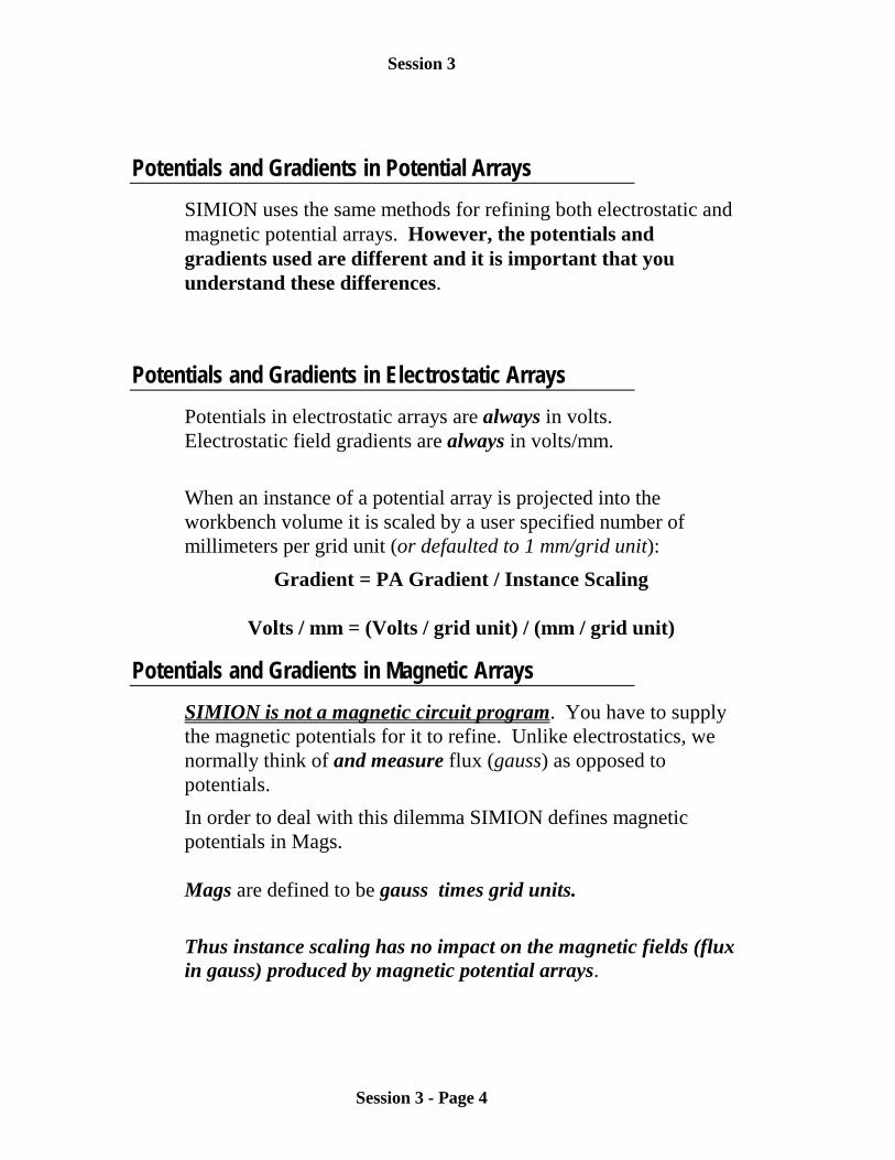
Potentials and Gradients in Potential ArraysSIMION uses the same methods for refining both electrostatic andmagnetic potential arrays. However, the potentials andgradients used are different and it is important that youunderstand these differences.

Potentials and Gradients in Electrostatic ArraysPotentials in electrostatic arrays are always in volts.Electrostatic field gradients are always in volts/mm.

When an instance of a potential array is projected into theworkbench volume it is scaled by a user specified number ofmillimeters per grid unit (or defaulted to 1 mm/grid unit):

Gradient = PA Gradient / Instance Scaling

Volts / mm = (Volts / grid unit) / (mm / grid unit)

Potentials and Gradients in Magnetic ArraysSIMION is not a magnetic circuit program. You have to supplythe magnetic potentials for it to refine. Unlike electrostatics, wenormally think of and measure flux (gauss) as opposed topotentials.In order to deal with this dilemma SIMION defines magneticpotentials in Mags.

Mags are defined to be gauss times grid units.

Thus instance scaling has no impact on the magnetic fields (fluxin gauss) produced by magnetic potential arrays.

Session 3

Session 3 - Page 5

The ng Magnetic Scaling FactorThe ng scaling factor has been provided to further simplify yourlife. It allows Mags to be directly related to gauss.Let's say we have a simple two pole magnet. We would like to setone pole to 1000 Mags and the other to Zero Mags and have thefield in between be approximately 1000 gauss. If the two polesare separated by let's say a 60 grid unit pole gap we would specifythe value of 60 for ng to automatically scale the Mags potentialsroughly into gauss.

PA Magnetic Flux = PA Magnetic Gradient (PA gauss)Magnetic Flux = PA Magnetic Flux * ng

gauss = PA gauss * ng (pole gap scaling factor)Note: The B field vector always points from greater magneticpotential (e.g. 1000 Mags) toward lesser magnetic potential (e.g. 0Mags).Beware! Magnetic poles do not as a rule have totally uniformmagnetic potentials across their surfaces (permeability not beinginfinite). Thus you must allow for this fact if the effects could besignificant enough to impact your results.

Adjusting Array Potentials

Modify the Potential(s) and Re-RefineThe first strategy is the brute force approach:1. Use the Modify function to change the potentials of the points

of one or more electrodes or poles in the potential array.2. The use the Refine function to re-refine the potential array to

obtain the resulting potentials of the non-electrode or non-polepoints.

This is the Modify-Refine cycle of array potential adjustment. Itis time consuming and invites errors (e.g. accidentally notchanging the potentials of all the points of an electrode or pole).

Session 3

Session 3 - Page 6

Proportional Re-scaling of All Array Potentials (.PAarrays)

SIMION 6.0 supports proportional re-scaling of all .PA arraypotentials. This is useful in those cases when the potentials of allelectrodes or poles can be changed proportionally to obtain thedesired result. This approach works with any simple array (with.PA file extension) that has already been refined:1. Use the Fast Adjust function to change the potential of the

highest potential electrode or pole in the potential array.2. SIMION will automatically scale the potentials of all array

points (electrode/pole and non) by the same proportion thatyou changed the potential of the highest potential electrode orpole.

Using Fast Adjust Arrays ( .PA# arrays)The third approach supported by SIMION makes use of theadditive solution property of the Laplace equation. Fortunately,SIMION is designed to do all the hard work for you!1. Use the Modify function to define the geometry of your

electrodes. All points of the first adjustable electrode/polemust be set to exactly 1 volt/Mag. Up to 30 adjustableelectrodes can be defined in this manner within a potentialarray.

2. Save this potential array with a .PA# file extension to signal toSIMION that this is a Fast Adjust Definition File (e.g. save asTEST.PA#).

3. Refine the .PA# file. SIMION will recognize that this is a FastAdjust Definition File and create, refine, and save eachrequired solution array automatically (.PA0 and so on). The.PA0 array is the base solution array (e.g. TEST.PA0).

4. Use the Fast Adjust function on the .PA0 file to set potentials .If you want to save the current potential settings of a .PA0file between SIMION sessions, simply save the .PA0 file todisk.

Session 3

Session 3 - Page 7

Session 3 - Lab on 2D Potential arrays - No After Installation Files Need to be Created


Creating and Refining a Simple Fast Adjust Electrostatic Array

1. Remove all PAs From RAM2. Use GUI File Manager to insert a directory called PROJECT below the \CLASS\SESSION3

directory and switch to this new directory.a. Click the GUI File Manager button (Main Menu Screen)b. Click on the \CLASS\SESSION3 directory (to switch to it)c. Click the Other button (to access other options)d. Enter PROJECT in the Create Directory ioline and press ENTER.e. Click on the \CLASS\SESSION3\PROJECT directory (to switch to it)f. Click the Use button to exit the GUI File Manager and stay in the currently selected

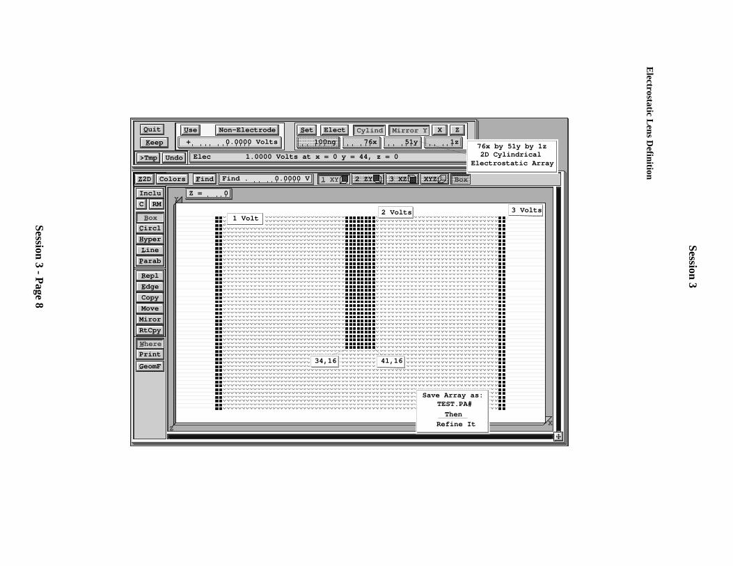
directory.3. Click the New button and create a 76x by 51y by 1z 2D cylindrical electrostatic array.4. Click the Modify button and use Modify to define the electrodes as show in the illustration below.

Note: If you have made an error in defining the array in Create you can change the definition fromwithin Modify (using the SET button - after making the desired definition changes).

5. When you’re satisfied that the results are OK, exit Modify by clicking the Keep button.6. The next task is to save the array as a fast adjust array (.PA#).

a. Click the Save button, and the GUI File Manager will appear.b. Make sure you are in the proper directory: \CLASS\SESSION3\PROJECT (click the

proper directory if needed).c. Enter the name TEST.PA# in the Filename ioline and Press ENTER.d. A file memo entry screen will appear. Either enter a short memo or press ENTER to skip

the memo.7. You will now be back on the Main Menu Screen. Click the REFINE button to enter the Refine

function.8. Click the Refine button on the Refine Screen and SIMION will create and refine all the required

fast adjust potential arrays.9. Now click the Fast Adjust button (on the Main Menu Screen). SIMION will automatically load

the TEST.PA0 file (your base solution file). Note: You could have loaded this file first via theOld or Load buttons.

10. Set the left and center electrodes to 1,000 volts and the right electrode to 0 volts. Now click theFast Adjust button to change the potentials in the TEST.PA0 array.

11. You will now be back on the Main Menu Screen. Click the View button to enter the Viewfunction. SIMION will automatically create a workbench volume the size of the potential array(TEST.PA0) assuming one mm per grid unit scaling.

12. Use various view orientations to look at the array including potential energy views.13. Click the Define button on the Normal Options Screen to access ion definitions. Create a group of

11 positively charged ions (blue) that start at x = 1 y = -5 (dy of + 1) with an energy of 0.01 eV.14. Click the OK button to return to View and fly the ions. They should focus. This is a converging

acceleration lens.15. Click the Define button on the Normal Options Screen to access ion definitions again.16. Click the Copy Grp button and then the Paste Grp button to create a copy of the current ion group.17. Change the color of the second ion group to red, its charge to minus one, and the starting energy to

1050 eV.18. Click the OK button and re-fly the ions. Use the PE view to see the negative ion surface. The

positive ions see this lens as a converging acceleration lens, while the negative ions see this lens asa diverging deceleration lens.

19. Now click the PAs tab to access the PAs Option Screen. Click the Fast Adjust button and changethe center electrode potential to zero volts. Re-fly the ions view the results. You now have adiverging acceleration for positive ions and a converging acceleration for negative ions.

Session 3

Session 3 - Page 8

Electrostatic Lens Definition

Use Non-Electrode

+ 0.0000 Volts

Set Elect Cylind Mirror Y X Z

100ng 76x 51y 1z

Quit

Keep

>Tmp Undo Elec 1.0000 Volts at x = 0 y = 44, z = 0

Z2D Colors Find Find . 0.0000 V 1 XY 2 ZY 3 XZ XYZ Box

Inclu

C RM

Box

Circl

Hyper

Line

Parab

Repl

Edge

Copy

Move

Miror

RtCpy

Where

Print

GeomF

Y

XZ

Z = 0Z = 0

76x by 51y by 1z2D Cylindrical

Electrostatic Array

1 Volt

34,16 41,16

2 Volts 3 Volts

Save Array as:TEST.PA#

Then

Refine It

Session 3

Session 3 - Page 9

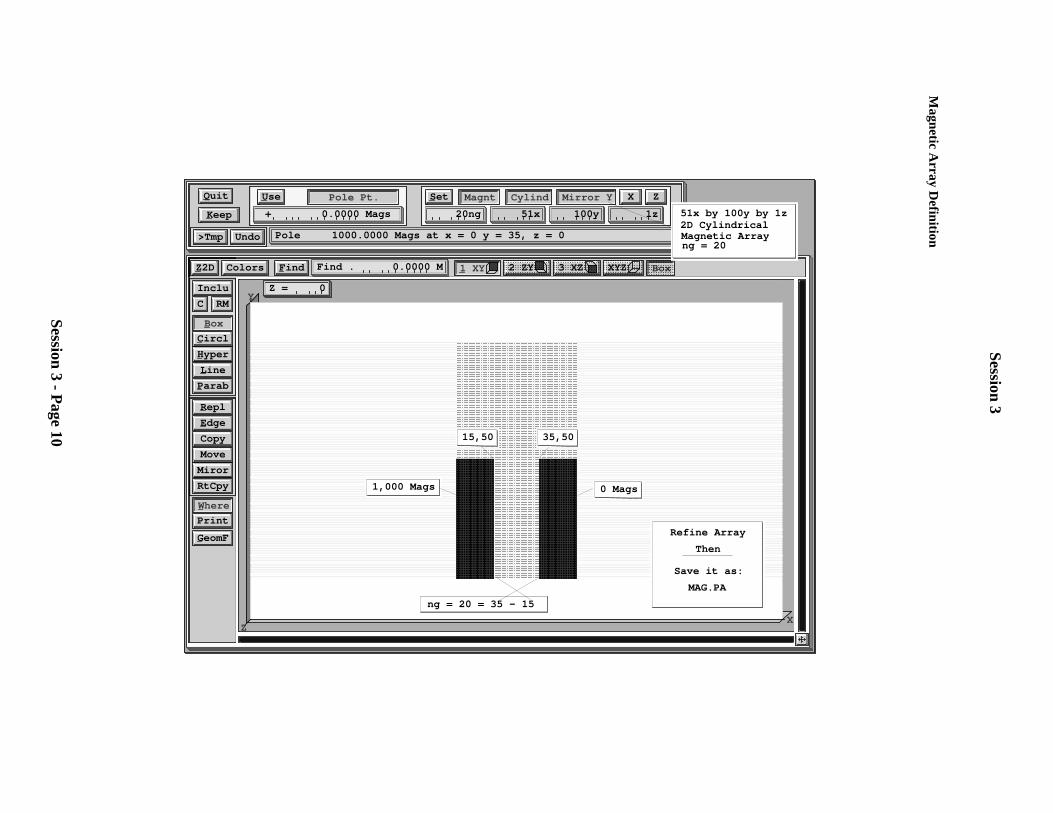
Creating and Refining a Magnetic Potential Array

1. Remove all PAs From RAM2. Click the New button and create a 51x by 100y by 1z 2D cylindrical magnetic array with ng = 20

(we plan to have a 20 grid unit pole gap).3. Click the Modify button and use Modify to define the poles as show in the illustration below.

Note: If you have made an error in defining the array in New you can change the definition fromwithin Modify (using the SET button - after making the desired definition changes).

4. When you’re satisfied that the results are OK, exit Modify by clicking the Keep button.5. Now use Refine to refine the array (remember this is a normal PA not a fast adjust definition

array).6. Since this is not a Fast Adjust array we must save the refining results to keep them between

sessions. Click the Save button and save the magnetic array as MAG.PA.7. Enter View and look at the array.8. One pole is 1,000 Mags, the other is 0 Mags, the pole separation is 20 gird units, and the value for

ng is 20. Move the cursor to the center of the magnet and verify that the field intensity is 1,000gauss. Note that the field intensity decreases quickly as you exit area between the poles.

9. Now try to define a group of 1,000 eV ions that pass between the poles and are bent by themagnetic field. This may take more effort than you expect because of the orientation of thepotential array ( the x, y, and z workbench directions align with the array by default).

10. Once you get ions flying through the magnet use the Fast Adjust button on the PAs Option Screento fast scale the field to some other field intensity and re-fly the ions.

11. You might also want to try expanding the workbench volume by clicking on the WrkBnch Tab andadjusting its size - be brave.

Session 3

Session 3 - Page 10

Magnetic A

rray Definition

Use Pole Pt.

+ 0.0000 Mags

Set Magnt Cylind Mirror Y X Z

20ng 51x 100y 1z

Quit

Keep

>Tmp Undo Pole 1000.0000 Mags at x = 0 y = 35, z = 0

Z2D Colors Find Find . 0.0000 M 1 XY 2 ZY 3 XZ XYZ Box

Inclu

C RM

Box

Circl

Hyper

Line

Parab

Repl

Edge

Copy

Move

Miror

RtCpy

Where

Print

GeomF

Y

XZ

Z = 0Z = 0

51x by 100y by 1z2D CylindricalMagnetic Arrayng = 20

15,50 35,50

0 Mags1,000 Mags

Refine Array

Then

Save it as:

MAG.PA

ng = 20 = 35 - 15

Session 3

Session 3 - Page 11

Demo of Using a Geometry File to Create an Array

1. Remove all PAs From RAM2. Click the New button.3. Click the Use Geometry File button and the GUI File Manager will appear.4. Switch to the \CLASS\SESSION3 directory.5. Click both mouse buttons on the MAGNET.GEM button to select and use it. SIMION will load

and use the definitions in this .GEM file to create the same magnetic array you created in theexample above.

6. Click the Modify button to verify that the array and its pole definitions were defined properly.7. Let’s now take a quick look at a geometry file:

a. Click the GeomF button on the Modify Screen to access the Geometry file developmentsystem.

b. Click the Edit button to load the MAGNET.GEM file into the EDY editor.c. Look at the file. These commands created and defined the potential array. More of this

tomorrow.d. Hit ESC then Q then N to exit the EDY editor.e. Click the Quit button to return to the Modify Screen.

8. Click the Keep button to keep the array and exit Modify.9. Refine the array (it is a simple .PA array).10. Save the array as MAGNET.PA (needed to save solutions for use by .IOB file).11. Remove all PAs from RAM.12. Click the View button and load MAGNET.IOB and restore potentials.13. Click the Define button (within View) and load the MAGNET.FLY ion definition file.14. Click OK to return to View and fly the ions.15. This is an example of what is known as Z focusing. The entry points of the ions control whether

they are focused or defocused in the z direction.

More for the Swift

Note that the orientation of the magnetic array is better in the demo than what you had. This is because theinstance definition specified a different orientation. To examine it:

1. Click the PAs Tab.2. Click the Edit button. You are now looking at the first instance editing screen. Things like

scaling, offsets and integral orientations appear on this screen.3. Click the More button to see the second instance edit screen. Note that orientation of the array has

been swung 90 degrees in the azimuth direction. Moreover the working origin of the potentialarray has been shifted a +25 grid units so that it is in the center between the two poles.

4. You should change this or that and see what happens. Leap!

Session 3

Session 3 - Page 12

This Page Intentionally Left blank

Session 4

Session 4 - Page 1

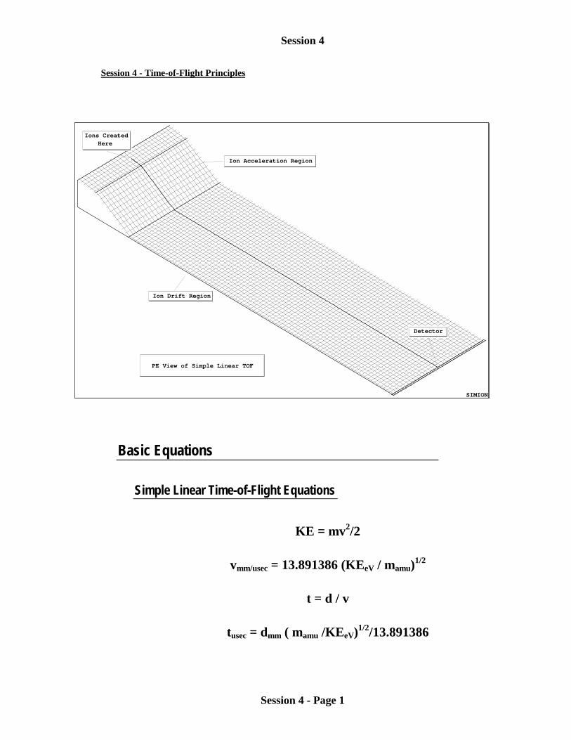
Session 4 - Time-of-Flight Principles

Basic Equations

Simple Linear Time-of-Flight Equations

KE = mv2/2

vmm/usec = 13.891386 (KEeV / mamu)1/2

t = d / v

tusec = dmm ( mamu /KEeV)1/2/13.891386

SIMION

Ions CreatedHere

Ion Acceleration Region

Ion Drift Region

PE View of Simple Linear TOF

Detector

Session 4

Session 4 - Page 2

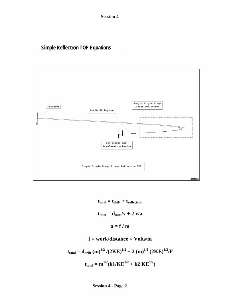
Simple Reflectron TOF Equations

ttotal = tdrift + treflectron

ttotal = ddrift/v + 2 v/a

a = f / m

f = work/distance = Volts/m

ttotal = ddrift (m)1/2 /(2KE)1/2 + 2 (m)1/2 (2KE)1/2/F

ttotal = m1/2(k1/KE1/2 + k2 KE1/2)

SIMION

Ion Source and

Acceleration Region

Simple Single StageLinear Reflectron

Ion Drift Regions

Detector

Simple Single Stage Linear Reflectron TOF

Session 4

Session 4 - Page 3

Session 4 - Lab on Time-of-Flight

This Lab’s Files are found in Directory: C:\CLASS\SESSION4\LINEAR

Flying Ions in a Simple Linear TOF

This model is used to demonstrate a very simple linear time-of-flight system. The demo makes use ofvoltage gradient time focusing for ions that are created at various locations in the ion formation region. Themodel is also used to demonstrate the use of the trajectory quality parameter to get proper discontinuitydetection.

Creating the Required Files After Installation (First Time Only)

a. Remove all PAs From RAMb. Use New and click the Use Geometry Files button. Use the LINEAR.GEM file by pointing to its

button and clicking both mouse buttons ( in C:\CLASS\SESSION4\LINEAR).c. Use the Save function to save the potential array as LINEAR.PA#.d. Use the Refine function on LINEAR.PA# to create the required files for the demo.

Lab Steps Assuming the Required Files Have Been Created

1. Remove all PAs From RAM2. Use View to load LINEAR.IOB from directory C:\CLASS\SESSION4\LINEAR3. Load the ions in the LINEAR.FLY file.4. Set time markers on at 1.0 usec with their color set to 15 (so the ion’s markers use the same color

as the ion’s trajectories).5. Load the data recording file LINEAR.REC and turn data recording on.6. Fly the ions singly with trajectory quality set to 2 (default value). Note the KE error. This value is

too large. The ions must be missing a grid edge.7. Re-fly the ions with increasing trajectory qualities (>2) until the KE error is around 10-6 or less.

Notice that the error suddenly improves between two successive values of data quality. This isbecause the CV detection is now just sensitive enough to see the grid edge. Notice theimprovement in the TOF times (on the data recording screen).

8. Notice that although the ions are created in different locations that they arrive at virtually the sametime. However, the compensation is not perfect. Can you explain why? Are we dealing withproblems with SIMION or basic physics?

9. Load and fly the ions in the LINEAR3.FLY file (25, 50, and 100 amu ions). Notice that all threeion masses bunch equally well.

10. Modify the data recording parameters so that the ion’s velocity is recorded when it splats. Are thevelocity ratios correct between ions of different masses? Are the ion’s velocities correct (use theequations above and check array potentials.

Session 4

Session 4 - Page 4

This Lab’s Files are found in Directory: C:\CLASS\SESSION4\REFLECT

Using the Single Stage Linear Reflectron Demo

This model is used to demonstrate a simple single stage linear reflectron time-of-flight system. The demomakes use of a single stage linear reflectron to time focus ions of the same mass but different kineticenergies.

No After Installation Files Need to be Created

1. Remove all PAs From RAM2. Use View to load TOF.IOB from directory C:\CLASS\SESSION4\REFLECT3. Load the ions in the TOF.FLY file.4. Load the data recording file TOF.REC and turn data recording on.5. Fly the ions grouped as dots. Note the arrival times on the data recording screen.6. Click the PAs tab, set the instance to one (the reflectron), and then click the Fast Adjust button.

Record the current reflectron potential (should be 1000 V). Now increase the reflectron potentialto 1500 volts and re-fly the ions. What happened? Now try 900 volts. Which ions get there first(low or higher energy)? Now try 1000.7 volts.

7. Select the detector instance (instance 3) on the PAs option screen. Click the Align button (leftedge of screen) to align the workbench coordinates with the detector. Now fly the ions. Zoom inand watch them hit the detector. The dot speed slider can be used. Also try the single stepfunction (just to the right of the trajectory quality panel - the Stp button).

8. Now go in and split the ion energies (was 50eV between two ions in each group) to 25 eV delta for3 ions in each group (increase the ions to 3 and change delta energy to 25 eV) for each of the twogroups. Re-fly the ions. What does your time focusing look like now? Explain what you see -physics or SIMION?

9. Reload the TOF.FLY ion definitions file, delete the second ion group, and now load theTIMES.REC data recording file. Fly the two ions and use the data recording information todetermine the ratio of drift time to time spent in the reflectron. The ratio should be 1.0 but it isn’t!What do you think is the cause? Hint: The acceleration stage creates a time shift.

10. To eliminate the impact of the ion acceleration stage, set its fast adjust voltage to zero (instance 2 -800 volts by default), and then set the first ion’s KE to 801 eV. Now re-fly the ions. Now they areno longer time focused!

11. We can pull the source further back from the reflectron to help the time focus. Make sure theAlign button is raised. Select instance 2 (the source instance). Now depress the Align button toalign the workbench coordinates with the working origin of the source array instance.

12. Click the Edit button on the PAs options screen. Move the source back by entering a negativevalue for Xwb (Hint: -91 is pretty close). The advantage of using the align function is that it allowsus to move the source along the ion’s flight path. Thus no beam alignment problems.

13. Now re-fly the ions and check splat time-of-flights. They should be pretty close if you used -91.14. Compare the drift time verses reflectron time ratios. They are very close to 1.0. If you fly an

intermediate energy ion (e.g. 3 ions with 25 eV delta KE), its time ratios will be very close to 1.0.

Session 4

Session 4 - Page 5

This Lab’s Files are found in Directory: C:\CLASS\SESSION4\FOCUS

How Refraction Impacts Time-of-Flight

This lab illustrates the errors in TOF introduced by the use of refractive elements like an einzel lens. A flatplane of ions entering an einzel lens does not leave as a flat plane of ions. However, the lab alsodemonstrates a trick that is useful to know.


1. Remove all PAs From RAM2. Use View to load EINZEL.IOB from directory C:\CLASS\SESSION4\FOCUS3. Load and fly the ions in the EINZEL.FLY. Set time markers on a 1.0 usec. with marker color set

to 15 (uses the ion’s color for marker color). Fly the ions singly as dots (fast - slider to right).4. Note that while the ions enter the lens as a vertical line of dots they do not leave the einzel that

way. Which ions are leading and which ions are trailing. What type of einzel is this, accel ordecel - use PE view as an aid.

5. Now fast adjust the center electrode to -250 volts and re-fly the ions. This is an accel einzel. Notethat the ion distortion is reversed. Can you explain why the ion trajectories are time distorted theway they are?

This leads to an idea! Why not use two einzels in series to focus the ions while compensating for the timedistortion by making one einzel an accel and the other a decel. If you want to test your skill with instances,go to the main menu, load the EINZEL.PA0 file and save it as EINZEL.PB0 (a second separate einzel fastadjust file). Remove all PAs from RAM and reload the EINZEL.IOB. Stretch the workspace to the right(increase xmax). Now mark where you want the second einzel to be, click the PAs tab, now the Add buttonand select the EINZEL.PB0 potential array. Use instance editing to scale and position this instanceproperly. Now make instance 2 an accel einzel and fly ions. If you play around with voltages the timefocusing problem can be pretty much eliminated.

If you’re not that ambitious run the two einzel demo:

1. Remove all PAs From RAM2. Use View to load FOCUS.IOB from directory C:\CLASS\SESSION4\FOCUS3. Load and fly the ions in the EINZEL.FLY. Set time markers on a 1.0 usec. with marker color set

to 15 (uses the ion’s color for marker color). Fly the ions singly as dots (fast - slider to right).4. Zoom into the group of dots near the focus point. Notice the that the time distortion is minimal. 5. Use various views to examine how the distortions are removed as the ions fly.

Session 4

Session 4 - Page 6

This page intentionally left blank

Session 5

Session 5 - Page 1

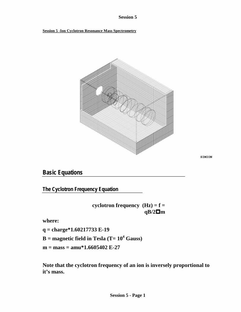
Session 5 -Ion Cyclotron Resonance Mass Spectrometry

SIMION

Basic Equations

The Cyclotron Frequency Equation

cyclotron frequency (Hz) = f =qB/2��m

where:q = charge*1.60217733 E-19B = magnetic field in Tesla (T= 104 Gauss)m = mass = amu*1.6605402 E-27

Note that the cyclotron frequency of an ion is inversely proportional toit’s mass.

Session 5

Session 5 - Page 2

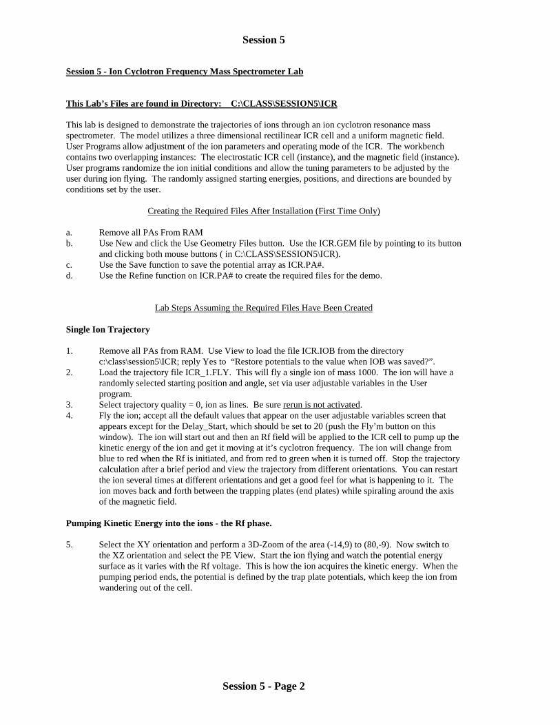
Session 5 - Ion Cyclotron Frequency Mass Spectrometer Lab

This Lab’s Files are found in Directory: C:\CLASS\SESSION5\ICR

This lab is designed to demonstrate the trajectories of ions through an ion cyclotron resonance massspectrometer. The model utilizes a three dimensional rectilinear ICR cell and a uniform magnetic field.User Programs allow adjustment of the ion parameters and operating mode of the ICR. The workbenchcontains two overlapping instances: The electrostatic ICR cell (instance), and the magnetic field (instance).User programs randomize the ion initial conditions and allow the tuning parameters to be adjusted by theuser during ion flying. The randomly assigned starting energies, positions, and directions are bounded byconditions set by the user.


a. Remove all PAs From RAMb. Use New and click the Use Geometry Files button. Use the ICR.GEM file by pointing to its button

and clicking both mouse buttons ( in C:\CLASS\SESSION5\ICR).c. Use the Save function to save the potential array as ICR.PA#.d. Use the Refine function on ICR.PA# to create the required files for the demo.


Single Ion Trajectory

1. Remove all PAs from RAM. Use View to load the file ICR.IOB from the directoryc:\class\session5\ICR; reply Yes to “Restore potentials to the value when IOB was saved?”.

2. Load the trajectory file ICR_1.FLY. This will fly a single ion of mass 1000. The ion will have arandomly selected starting position and angle, set via user adjustable variables in the Userprogram.

3. Select trajectory quality = 0, ion as lines. Be sure rerun is not activated.4. Fly the ion; accept all the default values that appear on the user adjustable variables screen that

appears except for the Delay_Start, which should be set to 20 (push the Fly’m button on thiswindow). The ion will start out and then an Rf field will be applied to the ICR cell to pump up thekinetic energy of the ion and get it moving at it’s cyclotron frequency. The ion will change fromblue to red when the Rf is initiated, and from red to green when it is turned off. Stop the trajectorycalculation after a brief period and view the trajectory from different orientations. You can restartthe ion several times at different orientations and get a good feel for what is happening to it. Theion moves back and forth between the trapping plates (end plates) while spiraling around the axisof the magnetic field.

Pumping Kinetic Energy into the ions - the Rf phase.

5. Select the XY orientation and perform a 3D-Zoom of the area (-14,9) to (80,-9). Now switch tothe XZ orientation and select the PE View. Start the ion flying and watch the potential energysurface as it varies with the Rf voltage. This is how the ion acquires the kinetic energy. When thepumping period ends, the potential is defined by the trap plate potentials, which keep the ion fromwandering out of the cell.

Session 5

Session 5 - Page 3

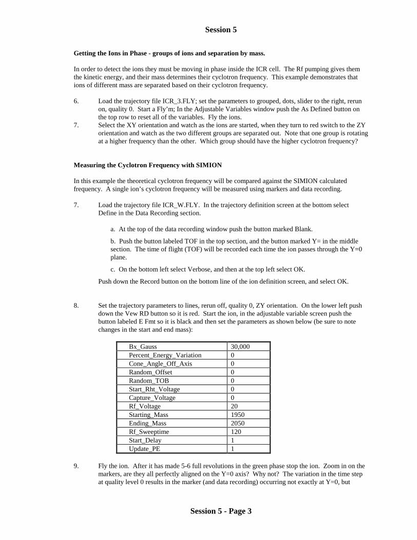
Getting the Ions in Phase - groups of ions and separation by mass.

In order to detect the ions they must be moving in phase inside the ICR cell. The Rf pumping gives themthe kinetic energy, and their mass determines their cyclotron frequency. This example demonstrates thations of different mass are separated based on their cyclotron frequency.

6. Load the trajectory file ICR_3.FLY; set the parameters to grouped, dots, slider to the right, rerunon, quality 0. Start a Fly’m; In the Adjustable Variables window push the As Defined button onthe top row to reset all of the variables. Fly the ions.

7. Select the XY orientation and watch as the ions are started, when they turn to red switch to the ZYorientation and watch as the two different groups are separated out. Note that one group is rotatingat a higher frequency than the other. Which group should have the higher cyclotron frequency?

Measuring the Cyclotron Frequency with SIMION

In this example the theoretical cyclotron frequency will be compared against the SIMION calculatedfrequency. A single ion’s cyclotron frequency will be measured using markers and data recording.

7. Load the trajectory file ICR_W.FLY. In the trajectory definition screen at the bottom selectDefine in the Data Recording section.

a. At the top of the data recording window push the button marked Blank.

b. Push the button labeled TOF in the top section, and the button marked Y= in the middlesection. The time of flight (TOF) will be recorded each time the ion passes through the Y=0plane.

c. On the bottom left select Verbose, and then at the top left select OK.

Push down the Record button on the bottom line of the ion definition screen, and select OK.

8. Set the trajectory parameters to lines, rerun off, quality 0, ZY orientation. On the lower left pushdown the Vew RD button so it is red. Start the ion, in the adjustable variable screen push thebutton labeled E Fmt so it is black and then set the parameters as shown below (be sure to notechanges in the start and end mass):

Bx_Gauss 30,000Percent_Energy_Variation 0Cone_Angle_Off_Axis 0Random_Offset 0Random_TOB 0Start_Rht_Voltage 0Capture_Voltage 0Rf_Voltage 20Starting_Mass 1950Ending_Mass 2050Rf_Sweeptime 120Start_Delay 1Update_PE 1

9. Fly the ion. After it has made 5-6 full revolutions in the green phase stop the ion. Zoom in on themarkers, are they all perfectly aligned on the Y=0 axis? Why not? The variation in the time stepat quality level 0 results in the marker (and data recording) occurring not exactly at Y=0, but

Session 5

Session 5 - Page 4

within the time step that includes Y=0. Thus the variation is dependent upon the length of the timesteps as the ions approach the Y=0 boundary.

10. Calculate the period for one revolution (using the numbers on the recording window). Thetheoretical cyclotron frequency for a 2000 amu ion in a 30,000 gauss field is 23.03417 kHz, howdoes this compare with the frequency measured using time markers? Calculate the ratio ofTheoretical/SIMION.

11. Set the quality to 2 and rerun the trajectory. Zoom in on the time markers, do they all align now?Why? With the quality level at 2 the program performs a binary boundary approach to the Y=0boundary. Recalculate the period and cyclotron frequency using the times in the data recordingwindow. How does this compare to the Theoretical value.

12. Rerun the ion, in the Adjustable Variable screen change the Bx_Gauss to 60,000 (double itsoriginal value). Now what is the cyclotron frequency, how did this affect the radius? How wouldyou use data recording to get a measurement of the radius?

Trapping ions formed outside the ICR cell

This example illustrates a method for trapping ions created outside the cell. Problems in trapping ions ofwidely varying mass due to their velocity differences are illustrated.

13. Load the ICR_4.FLY trajectories. Set to dots, grouped, slider to the right, quality 0, rerun on, XYorientation, and fly the ions. Use the As Defined user adjustable variable values and fly the ions.They will change color when the pump field comes on and when it is turned off. This works nicelyfor trapping these ions. What will happen when we have ions of widely varying mass?

14. Load the ICR_5.FLY trajectories and fly them as grouped dots with quality of 0, rerun on. Theions have been started with the same approximate kinetic energy (as set by the user definedvariable). Note that the heavier ions (red) are not moving as fast as the lighter ions (blue), and thatsome of the blue ions enter and leave the cell before the trapping voltage is applied. How wouldyou solve this problem?

Session 6

Session 6 - Page 1

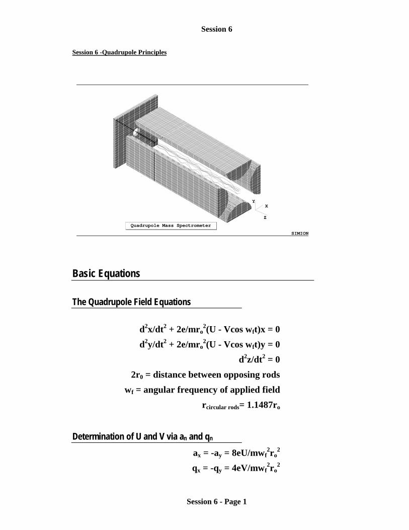
Session 6 -Quadrupole Principles

Basic Equations

The Quadrupole Field Equations

d2x/dt2 + 2e/mro2(U - Vcos wft)x = 0

d2y/dt2 + 2e/mro2(U - Vcos wft)y = 0

d2z/dt2 = 02r0 = distance between opposing rods

wf = angular frequency of applied fieldrcircular rods= 1.1487ro

Determination of U and V via an and qn

ax = -ay = 8eU/mwf2ro

2

qx = -qy = 4eV/mwf2ro

2

SIMION

Quadrupole Mass Spectrometer

XY

Z

Session 6

Session 6 - Page 2

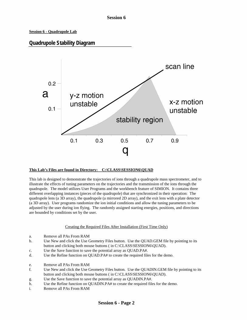
Session 6 - Quadrupole Lab

Quadrupole Stability Diagram

This Lab’s Files are found in Directory: C:\CLASS\SESSION6\QUAD

This lab is designed to demonstrate the trajectories of ions through a quadrupole mass spectrometer, and toillustrate the effects of tuning parameters on the trajectories and the transmission of the ions through thequadrupole. The model utilizes User Programs and the workbench feature of SIMION. It contains threedifferent overlapping instances (pieces of the quadrupole) that are synchronized in their operation: Thequadrupole lens (a 3D array), the quadrupole (a mirrored 2D array), and the exit lens with a plate detector(a 3D array). User programs randomize the ion initial conditions and allow the tuning parameters to beadjusted by the user during ion flying. The randomly assigned starting energies, positions, and directionsare bounded by conditions set by the user.


a. Remove all PAs From RAMb. Use New and click the Use Geometry Files button. Use the QUAD.GEM file by pointing to its

button and clicking both mouse buttons ( in C:\CLASS\SESSION6\QUAD).c. Use the Save function to save the potential array as QUAD.PA#.d. Use the Refine function on QUAD.PA# to create the required files for the demo.

e. Remove all PAs From RAMf. Use New and click the Use Geometry Files button. Use the QUADIN.GEM file by pointing to its

button and clicking both mouse buttons ( in C:\CLASS\SESSION6\QUAD).g. Use the Save function to save the potential array as QUADIN.PA#.h. Use the Refine function on QUADIN.PA# to create the required files for the demo.i. Remove all PAs From RAM

Session 6

Session 6 - Page 3

j. Use New and click the Use Geometry Files button. Use the QUADOUT.GEM file by pointing toits button and clicking both mouse buttons ( in C:\CLASS\SESSION6\QUAD).

k. Use the Save function to save the potential array as QUADOUT.PA#.l. Use the Refine function on QUADOUT.PA# to create the required files for the demo.


1. Remove all PAs from RAM. Use View to load the file QUAD.IOB from the directoryc:\class\session6\group; reply Yes to “Restore potentials to the value when IOB was saved?”.

2. Load the trajectory file QUAD.FLY. This will fly 25 ions of mass 100, the mass the quad is tunedto pass through. The ions will have randomly selected starting positions and angles, set via useradjustable variables in the User program.

3. Select trajectory quality = 0, ions as lines, ungrouped. Be sure rerun is not activated.4. Fly the ions; accept all the default values that appear on the user adjustable variables screen that

appears (push the Fly’m button on this window).5. View the ion trajectories using each view orientation, XY, ZY and XZ. In the XY view note the

nodes that appear in the trajectories. In the XY view make a 3D zoom from X=5 to X=85(leaving out the inlet and outlet optics), switch to ZY view and look at the trajectories.

6. In the ZY view make a cut that includes only the bottom and two side rods, switch to the 3D ISOview. Note the regions on the electrodes where the first instance interfaces with the second (thelong quad rods), and where the second instance (the long quad rods) interfaces with the exit region.

7. Exit from View (use the Quit button on the left). In the main menu screen select theQUADIN.PA0 array (push the button so it turns red), and then select Modify. This takes you intothe modify screen where you can see how the geometry was defined. Select the XYZ view, notethat is a planar array mirrored in Y and X. This saves array space (and memory!).

8. Leave Modify using the Quit button. Select the array QUAD.PA0 and look at it in Modify.What symmetries are used? Why? This is a simple 2D array, lots of space is saved by takingadvantage of the symmetries of this system.

9. Leave Modify using the Quit button. Select the array QUADOUT.PA0 and look at it in Modify.What symmetries are used here?

10. Leave Modify using the Quit button.11. Push the View button to return to the View screen. Push the PA tab and cycle through the

instances (upper left, blue panel), note they correspond to the three files you looked at in Modify.Instances can be added or deleted from the Workbench using the buttons on this window.

Mass Filtering - where do the ions go?

12. Load the trajectory file QUAD1.FLY. This file contains three sets of ions, one of mass 95 (belowthe quad tune point, color red), one set at mass 100 (the quad tune point, blue), and a third set atmass 105 (green). Again the ions are started at random angles and starting positions within thebounds set by the User Adjustable variables. Fly the ions and observe the trajectories.

13. View the trajectories in the ZY view, note which set of quadrupole rods the lighter ions impact,and which rods the heavier ions impact. Look at this from different views. Do any of the lighter orheavier ions make it to the detector?

14. One of the User Adjustable variables in the quadrupole axis voltage; this can be set on the screenthat appears after the Fly’m button is first pushed. Note the value (-8 volts) and run a set oftrajectories. Write down the approximate positions in X where the light and heavy ions hitthe rods. Now run the trajectories over and set the quadrupole axis voltage to -24 volts. How didthis affect where the ions hit the rods, did any of the ions make it to the detector? What does thistell you about how the axis voltage may affect the peak resolution, the peak shape, and the signalintensity.

15. Load in the QUAD.FLY trajectory file and fly the ions with the quadrupole axis voltage set to -8volts (default value), and in the XY view note the nodes that appear in the trajectories. Now re-flythe ions with this voltage set to -2 volts. How did this change the general shape of the trajectories,

Session 6

Session 6 - Page 4

how many nodes appear now? Try other values of this voltage, what happens if this voltage is setpositive? Could this be used to estimate the initial kinetic energy of the ions?

Ion Optics - how to get the ions into the quadrupole.

The effect of the ions’ trajectories as they enter the quad on the ion transmission is demonstrated. Dynamicdisplay of potential fields is shown, and the manner in which SIMION handles trajectories at interfacesbetween different instances is demonstrated.

16. Load the QUAD3.FLY trajectory file and fly the ions with the default User Adjustable values(hint, select the As Defined button). Now re-fly the ions with the User Adjustable variableCone_Angle_Off_Vel_Axis 15 degrees. What affect does this have, notice that now many ions arelost. The acceptance ellipse for the quad is finite and small, ions that enter outside of this are lost.

17. Load the QUAD1.FLY file. Run the ions as dots with the speed slider all the way to the right,grouped, with rerun on, be sure trajectory quality is set to 0. View in the XY and YZ planes.

18. Switch to the XY view and make a cut from X=0, Y=0 to X=10, Y=-9. Switch to the XZorientation and select PE View (potential energy surface). Set the drawing quality to 0 and theGstep to 5 or higher. Fly the ions and watch the PE surface undulate. Switch back to the WBview, select ZY orientation, switch back to PE view, and watch again as ions fly.

19. Stop the Fly’m. Switch back to WB view, select XY orientation, zoom out one level and nowmake a second cut so you have the region (0,0) to (18,-9) zoomed into. Switch to XZ orientationand select the PE view and fly the ions. Notice that only the left side of the field is changing, theright side is staying constant. What happens when the ions finally get into the field on the righthand side; what happens when there are no longer any ions in the left hand region? Recall that theworkbench has three instances in it, making up the quad. When does the program performcalculations for each instance? (Only when there are ions within the instance.) What happenswhen ions are in two instances?

20. Experiment with the effects of various tuning parameters (inlet and exit voltages etc), ionparameters (increase the energy spread, the position where ions are born) via the User DefinedVariables.

Session 7

Session 7 - Page 1

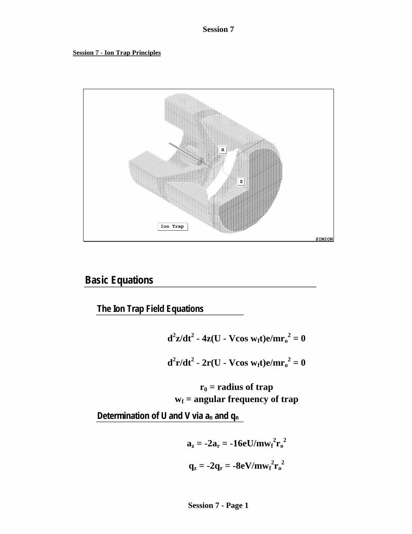
Session 7 - Ion Trap Principles

Basic Equations

The Ion Trap Field Equations

d2z/dt2 - 4z(U - Vcos wft)e/mro2 = 0

d2r/dt2 - 2r(U - Vcos wft)e/mro2 = 0

r0 = radius of trapwf = angular frequency of trap

Determination of U and V via an and qn

az = -2ar = -16eU/mwf2ro

2

qz = -2qr = -8eV/mwf2ro

2

SIMION

R

Z

Ion Trap

Session 7

Session 7 - Page 2

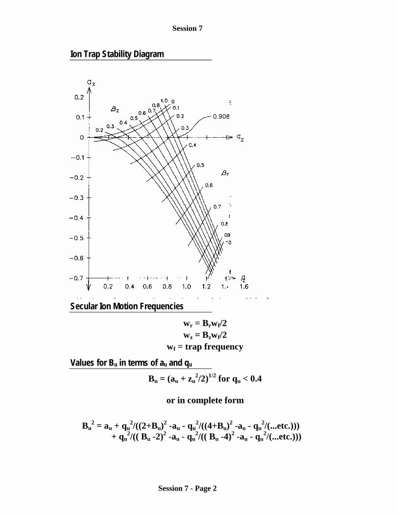
Ion Trap Stability Diagram

Secular Ion Motion Frequencies

wr = Brwf/2wz = Bzwf/2

wf = trap frequency

Values for Bu in terms of au and qu

Bu = (au + zu2/2)1/2 for qu < 0.4

or in complete form

Bu2 = au + qu

2/((2+Bu)2 -au - qu2/((4+Bu)2 -au - qu

2/(...etc.)))+ qu

2/(( Bu -2)2 -au - qu2/(( Bu -4)2 -au - qu

2/(...etc.)))

Session 7

Session 7 - Page 3

Session 7 - Lab on Ion Trap

This Lab’s Files are found in Directory: C:\CLASS\SESSION7\GROUP

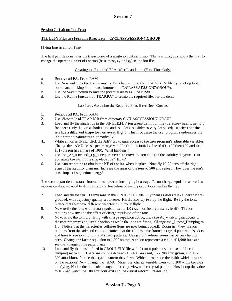
Flying Ions in an Ion Trap

The first part demonstrates the trajectories of a single ion within a trap. The user programs allow the user tochange the operating point of the trap (base mass, az, and qz) as the ion flies.


a. Remove all PAs From RAMb. Use New and click the Use Geometry Files button. Use the TRAP2.GEM file by pointing to its

button and clicking both mouse buttons ( in C:\CLASS\SESSION7\GROUP).c. Use the Save function to save the potential array as TRAP.PA#.d. Use the Refine function on TRAP.PA# to create the required files for the demo.


1. Remove all PAs From RAM2. Use View to load TRAP.IOB from directory C:\CLASS\SESSION7\GROUP3. Load and fly the single ion in the SINGLE.FLY ion group definition file (trajectory quality set to 0

for speed). Fly the ion as both a line and as a dot (use slider to vary dot speed). Notice that theion has a different trajectory on every flight. This is because the user program randomizes theion’s starting parameters automatically!

4.. While an ion is flying, click the AdjV tab to gain access to the user program’s adjustable variables.Change the _AMU_Mass_per_charge variable from its initial value of 40 to 90 then 100 and then101 (the ion has a mass of 100). What happens ?

5. Use the _Az_tune and _Qz_tune parameters to move the ion about in the stability diagram. Canyou make the ion hit the ring electrode? How?

6. Use data recording to obtain the KE of the ion when it splats. Now fly 10-20 ions off the rightedge of the stability diagram. Increase the mass of the ions to 500 and repeat. How does the ion’smass impact its ejection energy?

The second part demonstrates interactions between ions flying in a trap. Factor charge repulsion as well asviscous cooling are used to demonstrate the formation of ion crystal patterns within the trap.

7. Load and fly the ten 100 amu ions in the GROUP.FLY file. Fly them as dots (fast - slider to right),grouped, with trajectory quality set to zero. Hit the Esc key to stop the flight. Re-fly the ions.Notice that they have different trajectories in every flight.

8. Now re-fly the ions with factor repulsion set to 1.0 (each ion just represents itself). The ionmotions now include the effect of charge repulsion of the ions.

9. Now, while the ions are flying with charge repulsion active, click the AdjV tab to gain access tothe user program’s adjustable variables while the ions are flying. Change the _Linear_Damping to1.0. Notice that the trajectories collapse (ions are now being cooled). Zoom in. View the ionmotions from the side and end-on. Notice that the 10 ions have formed a crystal pattern. Use dotsand lines to see ion motions and streak patterns. Using a 3D volume zoom can be very helpfulhere. Change the factor repulsion to 1,000 so that each ion represents a cloud of 1,000 ions andsee the change in the pattern size.

10. Load and fly the ions defined in GROUP.FLY file with factor repulsion set to 1.0 and lineardamping set to 1.0. There are 45 ions defined (15 -100 amu red, 15 - 200 amu green, and 15 -300 amu blue). Notice the crystal pattern they form. Which ions are on the inside which ions areon the outside? Now change the _AMU_Mass_per_charge variable from 40 to 100 while the ionsare flying. Notice the dramatic change in the edge view of the crystal pattern. Now bump the valueto 102 and watch the 100 amu ions exit and the crystal reform. Interesting.

Session 7

Session 7 - Page 4

This Lab’s Files are found in Directory: C:\CLASS\SESSION7\TICKLE

Using the End Cap AC Voltages to Excite Selected Ions

If the end caps have a tickle voltage that has the secular frequency wz of specific ions’ mass for that a and qvalue the ions will gain energy and tend to leave the trap through the end cap holes. The user programs inthis demo compute the proper tickle frequency and allow the user to change the tickle voltage and otherparameters while the ions are flying. This demo also makes use of a collisional cooling model that usesmean free path and the mass of the cooling gas to simulate random collisional cooling of the ions.



button and clicking both mouse buttons ( in C:\CLASS|SESSION7\TICKLE).c. Use the Save function to save the potential array as TRAP.PA#.d. Use the Refine function on TRAP.PA# to create the required files for the demo.


1. Remove all PAs From RAM2. Use View to load TRAP.IOB from directory C:\CLASS\SESSION7\TICKLE3. Load and fly the ions in the TICKLE1.FLY (trajectory quality set to 0 for speed). Fly the ion as

grouped as dots (fast - slider to right). One group of ions (black) are not affected (mass not inresonance). However, the other group of ions (blue - red) will eventually be blown out of the trap.Notice that these ions change from blue to red. The user program does this to indicate the polarityof the tickle voltage being placed on the end caps. This shows that forcing being applied to theions.

4. Load and fly the ions in the TICKLE.FLY file (resonance ions only). Increase the tickle voltageand re-fly the ions.

5. Change the _AMU_Mass_per_charge variable from 40 to 80, re-fly and see what happens. Tryflying ions with this variable set to 10 amu. Can you explain what you see?

6. Change the _AMU_Mass_per_charge variable from to 303, tickle to zero volts, and re-fly. Nowturn on 2.0 volts of tickle while the ions are flying. This is an example of using tickle on the rightstability edge to help eject ions.

7. This model makes use of a collisional cooling model based on mean free path assumptionscontrolling random collisions with a bath gas of a given mass (helium - 4 by default). Change themean free path to 1 mm and see what effect increased gas pressure has on the tickle. Note settingmean free path to zero will turn off collisional damping.

8. You can also use the TRAP1.GEM file to create a new TRAP.PA# file with hole in left end capand a grid over the hole in the right end cap. Save the array, refine it, remove all PAs, reload theTRAP.IOB with View, and examine the impact of hole symmetry in the end caps on the preferredend cap for ion exit of the trap.

Session 7

Session 7 - Page 5

This Lab’s Files are found in Directory: C:\CLASS\SESSION7\INJECT

Injecting Ions into an Ion Trap

This demo models the injection of ions into an ion trap. 100 Ions are injected singly and the user programsperform a Monte Carlo analysis of each ion’s fate. The model makes use of collisional cooling with meanfree path and the mass of the cooling gas. It also includes an estimate of the reduction of the mean free pathas a function of the ion’s mass (and assumed complexity - cow pie effect):

mfpest = mfp/(1 + (n-1) _Avg_Visibility)Where:

n = ion mass / _Avg_Mass_per_atom_Avg_Mass_per_atom = 12 (default)_Avg_Visibility = 0.666 (default)



button and clicking both mouse buttons ( in C:\CLASS|SESSION7\INJECT).c. Use the Save function to save the potential array as TRAP.PA#.d. Use the Refine function on TRAP.PA# to create the required files for the demo.


1. Remove all PAs From RAM2. Use View to load TRAP.IOB from directory C:\CLASS\SESSION7\INJECT3. Load and fly the ions in the INJECT.FLY (trajectory quality set to 0 for speed). Fly the ion as

singly as dots (fast - slider to right). Fly about 30 ions and hit Esc to quit. Note the number of ionsactually trapped (from the data screen).

4. The mean free path is set to 40 mm (approx 10-4 torr). Decrease the mean free path to 4 mm andre-fly the ions. Are the results what you expected?

5. Now change the mass of the ions from 100 (their default) to 500, mean free path to 40, and rerun30 or so ions. How many did you trap? Not too many! Now re-fly these ions with the_AMU_Mass_per_charge variable set to 60 amu. Compare the results. Can you explain what yousee?

6. You can also change the sample and focus ring potentials and see their impact on ion capture.Give the ions a lot of energy (sample potential) and see what happens.

7. You can also use the TRAP2.GEM file to create a new TRAP.PA# file with ideal grids across theend cap holes. Save the array, refine it, remove all PAs, reload the TRAP.IOB with View, andexamine the impact of grids. The options are endless.

Session 7

Session 7 - Page 6

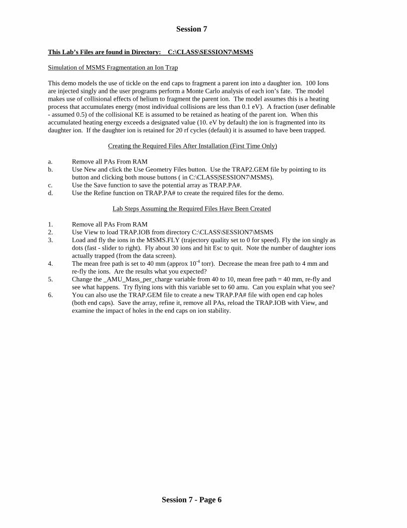
This Lab’s Files are found in Directory: C:\CLASS\SESSION7\MSMS

Simulation of MSMS Fragmentation an Ion Trap

This demo models the use of tickle on the end caps to fragment a parent ion into a daughter ion. 100 Ionsare injected singly and the user programs perform a Monte Carlo analysis of each ion’s fate. The modelmakes use of collisional effects of helium to fragment the parent ion. The model assumes this is a heatingprocess that accumulates energy (most individual collisions are less than 0.1 eV). A fraction (user definable- assumed 0.5) of the collisional KE is assumed to be retained as heating of the parent ion. When thisaccumulated heating energy exceeds a designated value (10. eV by default) the ion is fragmented into itsdaughter ion. If the daughter ion is retained for 20 rf cycles (default) it is assumed to have been trapped.



button and clicking both mouse buttons ( in C:\CLASS|SESSION7\MSMS).c. Use the Save function to save the potential array as TRAP.PA#.d. Use the Refine function on TRAP.PA# to create the required files for the demo.


1. Remove all PAs From RAM2. Use View to load TRAP.IOB from directory C:\CLASS\SESSION7\MSMS3. Load and fly the ions in the MSMS.FLY (trajectory quality set to 0 for speed). Fly the ion singly as

dots (fast - slider to right). Fly about 30 ions and hit Esc to quit. Note the number of daughter ionsactually trapped (from the data screen).

4. The mean free path is set to 40 mm (approx 10-4 torr). Decrease the mean free path to 4 mm andre-fly the ions. Are the results what you expected?

5. Change the _AMU_Mass_per_charge variable from 40 to 10, mean free path = 40 mm, re-fly andsee what happens. Try flying ions with this variable set to 60 amu. Can you explain what you see?

6. You can also use the TRAP.GEM file to create a new TRAP.PA# file with open end cap holes(both end caps). Save the array, refine it, remove all PAs, reload the TRAP.IOB with View, andexamine the impact of holes in the end caps on ion stability.

Session 9

Session 9 - Page 1

Session 9 - Geometry Files

What is a Geometry File

• A geometry file is an ASCII file with the .GEM filenameextension that contains the electrode/pole definitions for apotential array.

• It also may contain the definition of the potential array:

pa_define(100,20)

SIMION Functions that Use Geometry Files

• The New function via the Use Geometry File button (makes use ofpa_define commands).

• The Modify function via the GeomF button (ignores pa_definecommands for an existing array).

How Geometry Files Work

• The geometry files contain a collection of fill commands.

• Fill commands can define complex areas/volumes through the useof inclusion/exclusion commands (e.g. within and notin),orientation commands (e.g. locate), and large collection of basicshape commands (e.g. circle).

• Each successive fill command has increasing priority. Later fillcommands override earlier fill commands.

• SIMION makes use of a geometry compiler to create an orderedfill search tree.

• Each point within the array is checked to see if it is affected by afill command (from last fill toward first fill).

Session 9

Session 9 - Page 2

The Geometry File Language

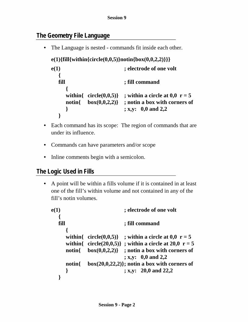
• The Language is nested - commands fit inside each other.

e(1){fill{within{circle(0,0,5)}notin{box(0,0,2,2)}}}e(1) ; electrode of one volt

{fill ; fill command

{within{ circle(0,0,5)} ; within a circle at 0,0 r = 5notin{ box(0,0,2,2)} ; notin a box with corners of} ; x,y: 0,0 and 2,2

}

• Each command has its scope: The region of commands that areunder its influence.

• Commands can have parameters and/or scope

• Inline comments begin with a semicolon.

The Logic Used in Fills

• A point will be within a fills volume if it is contained in at leastone of the fill’s within volume and not contained in any of thefill’s notin volumes.

e(1) ; electrode of one volt{fill ; fill command

{within{ circle(0,0,5)} ; within a circle at 0,0 r = 5within{ circle(20,0,5)} ; within a circle at 20,0 r = 5notin{ box(0,0,2,2)} ; notin a box with corners of

; x,y: 0,0 and 2,2notin{ box(20,0,22,2)}; notin a box with corners of} ; x,y: 20,0 and 22,2

}

Session 9

Session 9 - Page 3

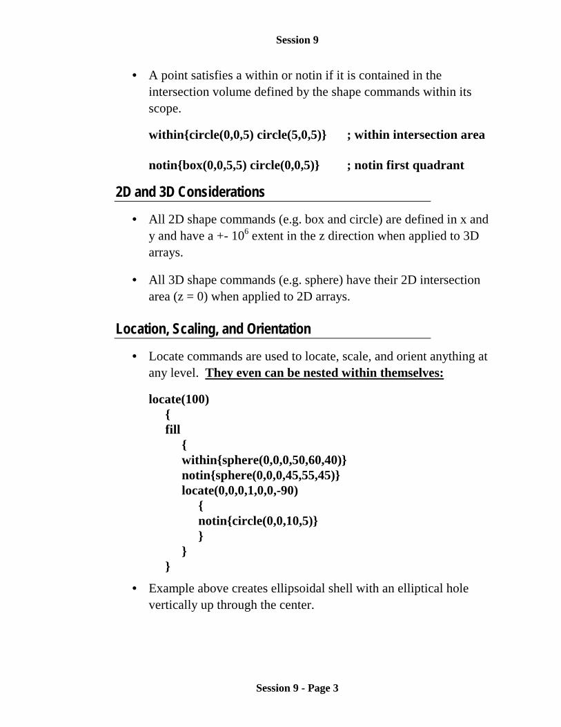
• A point satisfies a within or notin if it is contained in theintersection volume defined by the shape commands within itsscope.

within{circle(0,0,5) circle(5,0,5)} ; within intersection area

notin{box(0,0,5,5) circle(0,0,5)} ; notin first quadrant

2D and 3D Considerations

• All 2D shape commands (e.g. box and circle) are defined in x andy and have a +- 106 extent in the z direction when applied to 3Darrays.

• All 3D shape commands (e.g. sphere) have their 2D intersectionarea (z = 0) when applied to 2D arrays.

Location, Scaling, and Orientation

• Locate commands are used to locate, scale, and orient anything atany level. They even can be nested within themselves:

locate(100){fill

{within{sphere(0,0,0,50,60,40)}notin{sphere(0,0,0,45,55,45)}locate(0,0,0,1,0,0,-90)

{notin{circle(0,0,10,5)}}

}}

• Example above creates ellipsoidal shell with an elliptical holevertically up through the center.

Session 9

Session 9 - Page 4

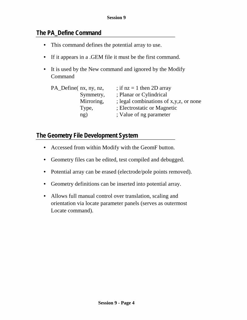
The PA_Define Command

• This command defines the potential array to use.

• If it appears in a .GEM file it must be the first command.

• It is used by the New command and ignored by the ModifyCommand

PA_Define( nx, ny, nz, ; if nz = 1 then 2D arraySymmetry, ; Planar or CylindricalMirroring, ; legal combinations of x,y,z, or noneType, ; Electrostatic or Magneticng) ; Value of ng parameter

The Geometry File Development System

• Accessed from within Modify with the GeomF button.

• Geometry files can be edited, test compiled and debugged.

• Potential array can be erased (electrode/pole points removed).

• Geometry definitions can be inserted into potential array.

• Allows full manual control over translation, scaling andorientation via locate parameter panels (serves as outermostLocate command).

Session 9

Session 9 - Page 5

Session 9 - Lab on Geometry Files

This Lab’s Files are found in Directory: C:\CLASS\SESSION9\TRAP

Inserting a Geometry File into Different Sized Arrays

The contents of a geometry file can be scaled to fit within arrays of different sizes. This lab shows how thisis done


1. Remove all PAs From RAM2. Use New to load TRAP.GEM from directory C:\CLASS\SESSION9\TRAP3. Examine the array with View and then Modify.4. The Array is 399x by 173y. Use Modify to halve the size of the array (200x by 87y);5. Click the GeomF button to access the geometry file development system.6. Test compile the geometry file by clicking the Compile button.7. Change the Scale panel from 1.0 (default) to 0.5 to re-scale the geometry definitions to the smaller

potential array.8. Click the Erase Entire PA button then click the Insert into PA button. You should now be looking

at the halved scale potential array.9. Follow the above steps 4-8 with the appropriate numbers to halve the array again. What can you

say about the change in resolution. Which array would you expect to model an ion trap moreaccurately?

10. Now we are going to insert this geometry file into a bigger array. In Modify, try to set a new arraysize of 797x by 345y. Did you have problems? What do you think is wrong? How would you fixit?

11. Remove all PAs From RAM12. Use New to define a cylindrical electrostatic 2D array with 797x by 345y coordinates (you will

have to increase the size of the Max PA to get these values).13. Now enter Modify and Click the GeomF button.14. Change the Scaling to 2.0 to double the geometry size to fit the new array.15. Click the Erase Entire PA button then click the Insert into PA button. You should now be looking

at the double scale potential array.16. Click the Keep button and enter View. There are a lot of points in this array. Change drawing

quality to 9 (click Esc if drawing takes too long).

Session 9

Session 9 - Page 6

This Lab’s Files are found in Directory: C:\CLASS\SESSION9\TRAP

Modifying the Trap Geometry File into a Stretched Trap

The contents of the trap geometry file above will be modified to define a Finnigan stretched trap which willbe saved as the STRETCH.GEM geometry file


1. Remove all PAs From RAM2. Use New to load TRAP.GEM from directory C:\CLASS\SESSION9\TRAP3. Examine the array with Modify.5. Click the GeomF button to access the geometry file development system.

6. Click the Edit button to edit the geometry file with EDY.7. Rename the File STRETCH.GEM

EDY keystrokes: Esc N STRETCH.GEM and press Enter8. Now Let’s save the file, exit EDY and Select and use this file as the geometry file:

Esc Q Y and your back in SIMION.9. Click the Select button and click both mouse buttons on STRETCH.GEM to make it the currently

selected .GEM file.10. Use the Erase all points button and then the Insert into PA button to verify that the geometry file

still makes the array OK.

11. Now the task is to shift both end caps 0.76 mm away from the trap center to create a stretched trap.The nominal scaling of this potential array is 0.1 mm/grid unit. Thus we need to shift the left endcap (and its contents) 7.6 grid units to the left and the right end cap 7.6 grid units to its right.

The best strategy is to insert locate commands that have the proper shifts and enclose the properelectrode definitions. This will result in the caps being shifted properly.

Go for it!

12. Assuming you’ve given it a good college try and failed. Use the Select button and click bothmouse buttons on the STRETCH1.GEM file. Insert the geometry from this file. It works! Look atthe file with EDY to see how it was done.

Session 9

Session 9 - Page 7

This Lab’s Files are found in Directory: C:\CLASS\SESSION9\EINZEL

Creating a geometry file for an EINZEL lens

A geometry file for an einzel lens will be created.


1. Remove all PAs From RAM2. Load the EINZEL.PA# array with Load3. Look at the electrode definitions with Modify.4. Write down, on paper, the image of a geometry file that would create the einzel array. Try to

include the proper PA_Define if you can. Seek the assistance of an instructor as necessary.5. Use New with the Use Geometry files button to access the file manager. Click the edit button to

access EDY.6. Name the file EINZEL.GEM with EDY:

Esc N EINZEL.GEM then ENTER7. Enter the contents into the file from the keyboard.8. Now Let’s save the file, exit EDY, and Select and use this file as the geometry file:

Esc Q Y and you’re back in SIMION.9. Click both buttons on the EINZEL.GEM file’s button.10. If all is OK the array will be created. If not, you will be informed.11. In any event, enter modify and see what you created.12. Click the GeomF button to begin to change or fix your geometry definitions

13. If you want to see a successful example, look at the EINZEL1.GEM file.

Session 9

Session 9 - Page 8

This page intentially left blank

Session 10

Session 10 - Page 1

Session 10 - User Programs

What is a User Program File

• A user program file is an ASCII file with the .PRG filenameextension that contains the user program segments for use with apotential array (.PA or .PA0).

• It shares the name of the potential array it supports. TEST.PRGwould automatically be used to support the TEST.PA array.

• User programs are associated with arrays not instances.

How SIMION Utilizes User Programs

• Each time the Fly’m button is clicked SIMION automaticallycompiles all user program files for any instances that have userprograms attached to their associated potential array.

• If Adjustable variables are found, the user will be given a screen toview and change their initial values.

• User program segments are called only when ions are flying withinthe array that the user program segments support.

User Program Segments

• The user program file contains user program segments.

• User program segments act like subroutines.

• SIMION calls each type of program segment at specific points in atrajectory calculation.

• Thus you must use a specific user program segment to control aspecific aspect of the trajectory calculation.

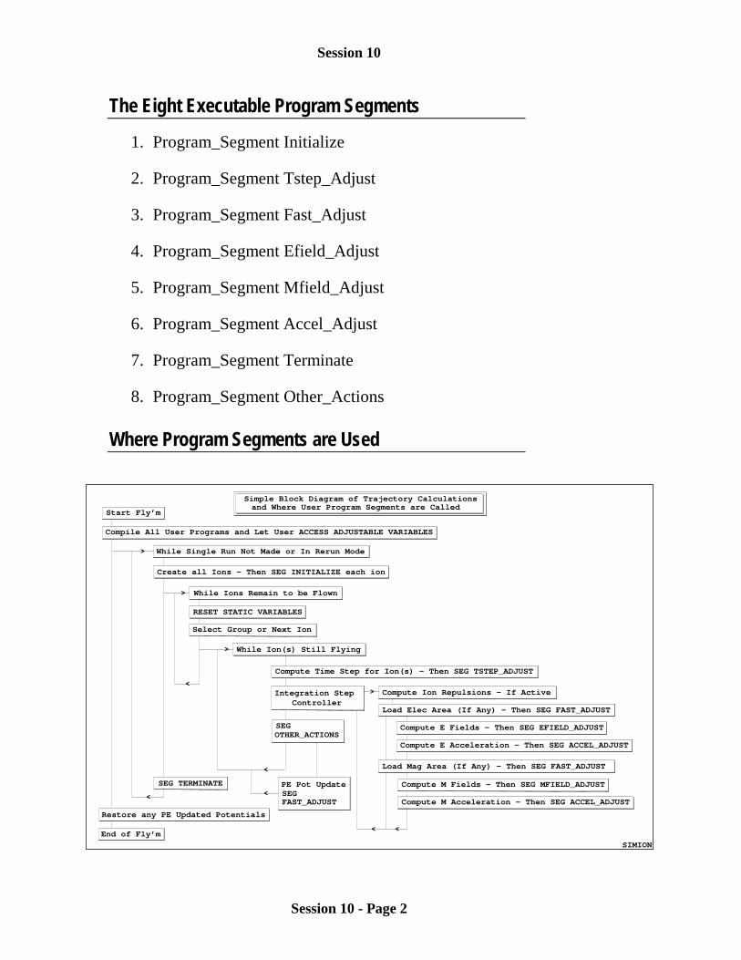
Session 10

Session 10 - Page 2

The Eight Executable Program Segments

1. Program_Segment Initialize

2. Program_Segment Tstep_Adjust

3. Program_Segment Fast_Adjust

4. Program_Segment Efield_Adjust

5. Program_Segment Mfield_Adjust

6. Program_Segment Accel_Adjust

7. Program_Segment Terminate

8. Program_Segment Other_Actions

Where Program Segments are Used

SIMION

Start Fly’m

Compile All User Programs and Let User ACCESS ADJUSTABLE VARIABLES

While Single Run Not Made or In Rerun Mode

Create all Ions - Then SEG INITIALIZE each ion

While Ions Remain to be Flown

Select Group or Next Ion

While Ion(s) Still Flying

Compute Time Step for Ion(s) - Then SEG TSTEP_ADJUST

RESET STATIC VARIABLES

Integration StepController

Compute Ion Repulsions - If Active

Load Elec Area (If Any) - Then SEG FAST_ADJUST

Compute E Fields - Then SEG EFIELD_ADJUST

Compute E Acceleration - Then SEG ACCEL_ADJUST

Load Mag Area (If Any) - Then SEG FAST_ADJUST

Compute M Fields - Then SEG MFIELD_ADJUST

Compute M Acceleration - Then SEG ACCEL_ADJUST

SEGOTHER_ACTIONS

SEG TERMINATE

End of Fly’m

PE Pot UpdateSEGFAST_ADJUST

>

>

>

< <

<

<

><

<

Restore any PE Updated Potentials

Simple Block Diagram of Trajectory Calculationsand Where User Program Segments are Called

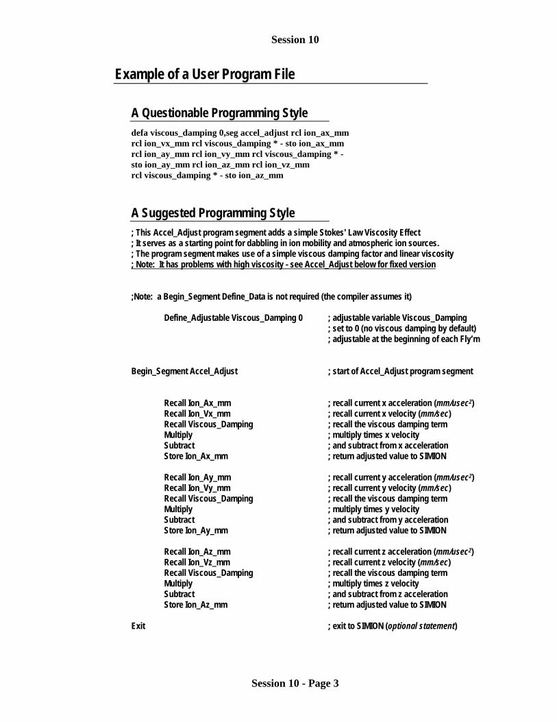
Session 10

Session 10 - Page 3

Example of a User Program File

A Questionable Programming Styledefa viscous_damping 0,seg accel_adjust rcl ion_ax_mmrcl ion_vx_mm rcl viscous_damping * - sto ion_ax_mmrcl ion_ay_mm rcl ion_vy_mm rcl viscous_damping * -sto ion_ay_mm rcl ion_az_mm rcl ion_vz_mmrcl viscous_damping * - sto ion_az_mm

A Suggested Programming Style; This Accel_Adjust program segment adds a simple Stokes' Law Viscosity Effect; It serves as a starting point for dabbling in ion mobility and atmospheric ion sources.; The program segment makes use of a simple viscous damping factor and linear viscosity; Note: It has problems with high viscosity - see Accel_Adjust below for fixed version

;Note: a Begin_Segment Define_Data is not required (the compiler assumes it)

Define_Adjustable Viscous_Damping 0 ; adjustable variable Viscous_Damping; set to 0 (no viscous damping by default); adjustable at the beginning of each Fly’m

Begin_Segment Accel_Adjust ; start of Accel_Adjust program segment

Recall Ion_Ax_mm ; recall current x acceleration (mm/usec2)Recall Ion_Vx_mm ; recall current x velocity (mm/sec)Recall Viscous_Damping ; recall the viscous damping termMultiply ; multiply times x velocitySubtract ; and subtract from x accelerationStore Ion_Ax_mm ; return adjusted value to SIMION

Recall Ion_Ay_mm ; recall current y acceleration (mm/usec2)Recall Ion_Vy_mm ; recall current y velocity (mm/sec)Recall Viscous_Damping ; recall the viscous damping termMultiply ; multiply times y velocitySubtract ; and subtract from y accelerationStore Ion_Ay_mm ; return adjusted value to SIMION

Recall Ion_Az_mm ; recall current z acceleration (mm/usec2)Recall Ion_Vz_mm ; recall current z velocity (mm/sec)Recall Viscous_Damping ; recall the viscous damping termMultiply ; multiply times z velocitySubtract ; and subtract from z accelerationStore Ion_Az_mm ; return adjusted value to SIMION

Exit ; exit to SIMION (optional statement)

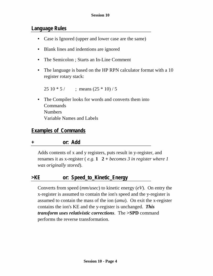
Session 10

Session 10 - Page 4

Language Rules

• Case is Ignored (upper and lower case are the same)

• Blank lines and indentions are ignored

• The Semicolon ; Starts an In-Line Comment

• The language is based on the HP RPN calculator format with a 10register rotary stack:

25 10 * 5 / ; means (25 * 10) / 5

• The Compiler looks for words and converts them intoCommandsNumbersVariable Names and Labels

Examples of Commands

+ or: Add

Adds contents of x and y registers, puts result in y-register, andrenames it as x-register ( e.g. 1 2 + becomes 3 in register where 1was originally stored).

>KE or: Speed_to_Kinetic_Energy

Converts from speed (mm/usec) to kinetic energy (eV). On entry thex-register is assumed to contain the ion's speed and the y-register isassumed to contain the mass of the ion (amu). On exit the x-registercontains the ion's KE and the y-register is unchanged. Thistransform uses relativistic corrections. The >SPD commandperforms the reverse transformation.

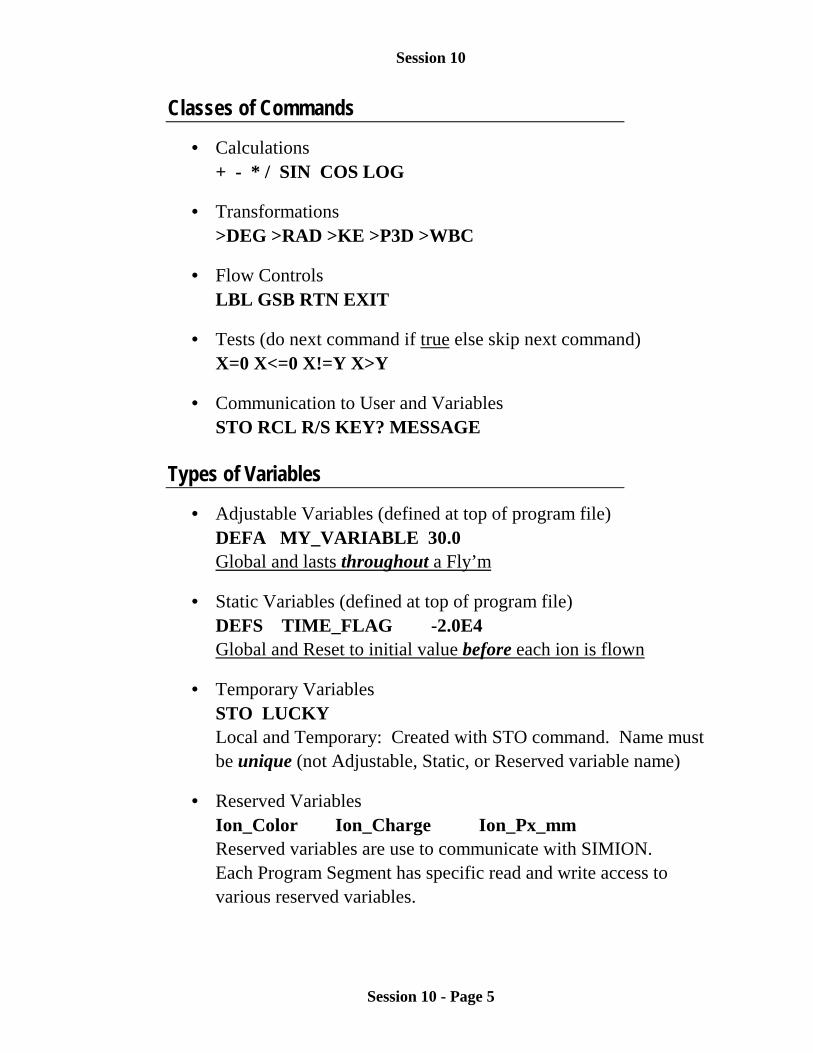
Session 10

Session 10 - Page 5

Classes of Commands

• Calculations+ - * / SIN COS LOG

• Transformations>DEG >RAD >KE >P3D >WBC

• Flow ControlsLBL GSB RTN EXIT

• Tests (do next command if true else skip next command)X=0 X<=0 X!=Y X>Y

• Communication to User and VariablesSTO RCL R/S KEY? MESSAGE

Types of Variables

• Adjustable Variables (defined at top of program file)DEFA MY_VARIABLE 30.0Global and lasts throughout a Fly’m

• Static Variables (defined at top of program file)DEFS TIME_FLAG -2.0E4Global and Reset to initial value before each ion is flown

• Temporary VariablesSTO LUCKYLocal and Temporary: Created with STO command. Name mustbe unique (not Adjustable, Static, or Reserved variable name)

• Reserved VariablesIon_Color Ion_Charge Ion_Px_mmReserved variables are use to communicate with SIMION.Each Program Segment has specific read and write access tovarious reserved variables.

Session 10

Session 10 - Page 6

Name Use Units Read Access Write AccessAdj_Elect01 toAdj_Elect30

Fast Adj ElectrodeVoltages

Volts Fast_Adjust Fast_Adjust

Adj_Pole01 toAdj_Pole30

Fast Adj PoleMag Potentials

Mags Fast_Adjust Fast_Adjust

Ion_Ax_mmIon_Ay_mmIon_Az_mm

Ion's currentAcceleration(WB Coordinates)

mm/micro sec2(WB Orientation)

Accel_AdjustOther_ActionsTerminate

Accel_Adjust

Ion_BfieldX_guIon_BfieldY_guIon_BfieldZ_gu

Magnetic Fieldat Ion's Location(PA's Orientation)

Gauss(PA's Orientation) Mfield_Adjust Mfield_Adjust

Ion_BfieldX_mmIon_BfieldY_mmIon_BfieldZ_mm

Magnetic Fieldat Ion's Location(WB Orientation)

Gauss(WB Orientation)

Accel_AdjustOther_ActionsTerminate

None

Ion_Charge Ion's current charge in units ofelementary charge

Any Prog Seg InitializeOther_Actions

Ion_Color Color of Ion 0-15 InitializeOther_Actions

InitializeOther_Actions

Ion_DvoltsX_guIon_DvoltsY_guIon_DvoltsZ_gu

Voltage Gradientat Ion's Location(PA's Orientation)

Volts/grid unit(PA's Orientation) Efield_Adjust Efield_Adjust

Ion_DvoltsX_mmIon_DvoltsY_mmIon_DvoltsZ_mm

Voltage Gradientat Ion's Location(WB Orientation)

Volts/mm(WB Orientation)

Mfield_AdjustAccel_AdjustOther_ActionsTerminate

None

Ion_Instance Current Instance 1- max instance Any Prog Seg NoneIon_Mass Ion's current mass amu Any Prog Seg Initialize

Other_ActionsIon_mm_Per_Grid_Unit Min Current Scaling1 mm/grid unit Any Prog Seg NoneIon_Number Ion's Number 1- max ion Any Prog Seg NoneIon_Px_Abs_guIon_Py_Abs_guIon_Pz_Abs_gu

Ion's current PAArray Coordinates

grid units(PA's AbsCoordinates)

Any Prog Seg None

Ion_Px_guIon_Py_guIon_Pz_gu

Ion's current(PA's Coordinates)

grid units(PA's Coordinates) Any Prog Seg None

Ion_Px_mmIon_Py_mmIon_Pz_mm

Ion's currentWorkbenchCoordinates

mm(WB Coordinates) Any Prog Seg


Ion_Splat Ion Status Flag2 Flying = 0Not Flying != 0



Ion_Time_of_Birth Ion's Birth Time micro seconds Any Prog Seg InitializeOther_Actions

Ion_Time_of_Flight Ion's current TOF3 micro seconds Any Prog Seg Other_ActionsIon_Time_Step Ion's Time Step4 micro seconds All but Initialize Tstep_Adjust

Ion_VoltsElectrostatic Potat Ion's Location Volts

Efield_AdjustMfield_AdjustAccel_AdjustOther_ActionsTerminate

Efield_Adjust

Ion_Vx_mmIon_Vy_mmIon_Vz_mm

Ion's currentVelocity(WB Coordinates)

mm/micro sec(WB Orientation) Any Prog Seg


Rerun_Flym Rerun Flym Flag NO = 0YES = 1

InitializeTerminate

InitializeTerminate

Update_PE_Surface New PE Surface5 YES != 0 None Other_Actions

Session 10

Session 10 - Page 7

Session 10 - Lab on User Programs

This Lab’s Files are found in Directory: C:\CLASS\SESSON10

Using an Existing User Program

The best way to start programming is to steal, steal, steal.

1. Remove all PAs From RAM2. Use New to create a new array using EINZEL.GEM from directory C:\CLASS\SESSON103. Save the array as EINZEL.PA# and then Refine it.4. Remove all PAs From RAM5. Use View to load EINZEL.IOB6. Use the Define button and load the EINZEL.FLY file.7. Fly the ions and see that they focus properly.

8. Now exit View and click on the GUI file manager button9. Click the Other button and enter the following command in the DOS ioline:

COPY RANDOM.PRG EINZEL.PRGand press the ENTER key (to create a copy of the user program with the EINZEL name).

10. Hit the Esc key several times to return to the main menu.11. Notice that the Test & Debug User program button is unblocked. SIMION has recognized that

there is now a user program associated with the EINZEL.PA0 potential array. Click the Test &Debug button access the user program development system (just a quick look).

12. Click the Compile button and the program will be compiled. If you want a cross reference listingdepress the Show Xref Listing button and then click the Compile button again. If you want to lookat this cross reference listing with EDY click the View: EINZEL.ERR button. Look at the listing.You can exit EDY by the following keystrokes: ESC Q N.

13. To examine the user program file with EDY click the Edit: EINZEL.PRG button. Look at thelisting. Exit EDY by the following keystrokes: ESC Q N.

14. Click the Compile button again to verify everything is OK. Now click the Quit key to return to themain menu.

15. Re-enter View and fly the ions. SIMION will compile the user programs and display theadjustable variables. Click the E Fmt button to switch from E to F format display. Now fly theions with the default settings. What a mess!

16. You can turn off the user programs for a single run. Click Fly’m and then Click the On button toturn the user program off, and then fly the ions.

17. Re-Fly the ions with various adjustable variable settings and see what happens. Are the resultsreasonable?

18. Perhaps you would like to change the starting values for the adjustable variables in the userprogram. Click the PAs tab and then the Debug button to access the user program developmentscreen. Now click the Edit button to access the user program file with EDY. Change the startingvalues of the adjustable variables. Now save the file and exit from EDY: ESC Q Y. Click theCompile button to check for compile errors. Now click the Quit button to return to View. Re-Flythe ions to confirm that the changes in initial value have been made successfully

Session 10

Session 10 - Page 8

Adding a User Program Segment

User programs generally develop by evolution. In this can we would like to exert some user control fromthe keyboard. The object is to create a marker every time a keyboard key is pressed. This is really a verysimple task.

1. Click the PAs tab and then the Debug button to access the user program development screen. Nowclick the Edit button to access the user program file with EDY.

2. Add the following two lines at the bottom of the file:

seg other_actionskey? x!=0 mark

The first line defines the start of an Other_Actions program segment. The second line has threecommands:key? Tests for keyboard input and returns a non-zero key code if you hit a keyx!=0 Tests the return value from key? for a non-zero value (you hit a key)

If the value is non-zero the next instruction will be executed (do if true) else itwill be skipped and the program segment will exit without doing anything.

mark This command creates a single marker. It uses the currently selected markercolor and can be used as a trigger event for data recording. The mark commandis executed if the x!=0 test is true.

3. Now save the changes and exit EDY: ESC Q Y. Test compile your efforts. If you have an errorfix it with EDY. Keep trying until it compiles OK. Now click the Quit button to return to View.

4. Fly the ions as dots with the speed slider to the center to slow the ions down a bit. Hit the spacebarand watch for markers. Can you create markers anywhere? What is the problem? Remember, anarray’s user program will only be called when ions are actually within its instance’s arrayvolume.

Additional Challenges

1. Modify the user program to output the ion’s x, y, and z position in workbench coordinates (mm)when you hit a key. Hint: The MESSAGE, LBL, GTO, and EXIT commands might be helpful.

2. Change this program to output x, y, and z in 3D array coordinates and then in absolute arraycoordinates.

3. For a real challenge calculate and display the ion’s KE when you hit a key. Hint: The >P3D and>KE transforms might be helpful.

Documents

Ion Optics Through the Eyes of SIMION 6simion.com/docs/class-handout.pdf · · 2009-11-24Ion Optics Through the Eyes of SIMION 6.0 AN ASMS SHORT COURSE ... Run EINZEL Demo Clear