Embed Size (px)
Citation preview
1
Ionosphere Threat to LAAS: Updated Model, User Impact, and Mitigations
Ming Luo, Sam Pullen, Alexandru Ene, Di Qiu, Todd Walter, and Per Enge
Stanford University
ABSTRACT
Several severe ionosphere storms have occurred in recent years that tripped the WAAS storm detector and caused partial WAAS service shutdowns. Under extreme conditions, these spatial gradients can threaten LAAS. In previous work [1-4], a “linear spatial gradient front” model was established and a threat space was extrapolated based on data from the 6 April 2000 ionospheric storm. User vertical error was estimated based on this threat model. The mitigating impact of LAAS Ground Facility (LGF) and airborne monitoring was also analyzed. Although those monitors can detect a “moving front” scenario, the so-called “stationary front” scenario remains threatening since the LGF may never be able to observe it (e.g., if the ionosphere front stops moving at the worst possible location prior to reaching the LGF.) It was shown that a ground-based Long Baseline Monitor (LBM) is able to mitigate such a threat if the baseline is set appropriately [5]. However, the cost and complexity of LBM deployment would be severe.
Although the worst-case ionosphere anomaly poses a serious concern, it is unclear what the prior probability of these extreme events may be, how credible the boundary of threat space is, and to what extent the threat model captures possible ionosphere storm behavior. In order to answer those questions, additional data analysis has been performed to better determine the credibility of the ionosphere spatial anomaly threat space. Recent CONUS ionospheric storms (using WAAS and JPL IGS/CORS data during October and November 2003) were studied thoroughly. The ionosphere threat model has been modified based on this new data. Instead of being extrapolated from a single observed anomaly as the previous model, the revised threat space is populated with many more observed data points.
In this paper, the threat of ionosphere spatial anomaly to LAAS is analyzed based on the revised model. The worst-case user vertical error and tolerable threat space are simulated with LGF and LGF-plus-airborne monitoring under various satellite constellations. The effectiveness of airborne monitoring is examined. When monitors are not sufficient to mitigate the potential threat, geometry screening is introduced as the final resource to protect integrity (the result is a loss of availability). Three methods are described and compared for geometry screening: real-time ionosphere error simulation, Lmax screening, and VPLH0 screening. Availability assessment
is performed for both monitoring conditions with various Vertical Alert Limits (VALs). Finally, a possible solution is suggested to protect integrity under ionosphere threat without changing the current CAT I LAAS architecture.
1.0 INTRODUCTION
The ionosphere is a dispersive medium located in the region of the upper atmosphere between about 50 km to about 1000 km above the Earth [6]. The radiation of the Sun produces free electrons and ions that cause phase advance and group delay in radio waves. The state of the ionosphere is a function of the intensity of solar activity, magnetic latitude, local time, and other factors. As GPS signals traverse the ionosphere, they are delayed by an amount proportional to the Total Electron Content (TEC) within the ionosphere at a given time. Because the ionosphere is constantly changing, the error introduced by the ionosphere into the GPS signal is highly variable and is difficult to model at the level of precision needed for LAAS. However, under nominal conditions, the spatial gradient is at the range of 2 − 5 mm/km (1σ), and the LAAS user error is small (less than 10 cm, 1σ).
The possibility of extremely large ionosphere spatial gradients was originally discovered in the study of WAAS “supertruth” (post-processed, bias-corrected) data during ionosphere storm events at the time of the last solar maximum (2000 − 2001). It was estimated that an ionosphere storm on 6 April 2000 resulted in a 7 m differential delay over the IPP separation of 19 km. This translates into an ionosphere delay rate of change of approximately 316 mm/km, which is two magnitudes higher than the typical one-sigma ionosphere vertical gradient value identified previously. Since a Gaussian extrapolation of the 5 mm/km one-sigma number does not come close to overbounding this extreme gradient, and because it is impractical to dramatically increase the broadcast one-sigma number without losing all system availability, we must treat this event as an anomaly and detect and exclude cases of it that lead to hazardous user errors. The detailed study on the 6 April 2000 storm can be found in [1].
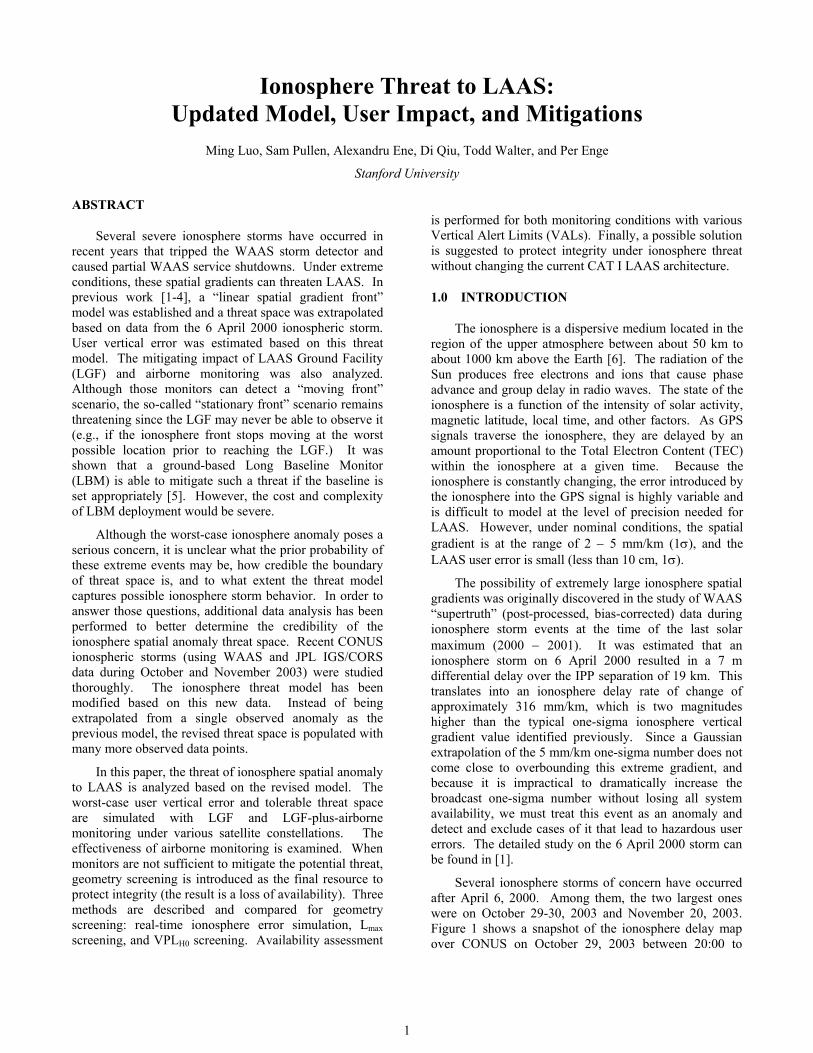
Several ionosphere storms of concern have occurred after April 6, 2000. Among them, the two largest ones were on October 29-30, 2003 and November 20, 2003. Figure 1 shows a snapshot of the ionosphere delay map over CONUS on October 29, 2003 between 20:00 to
2
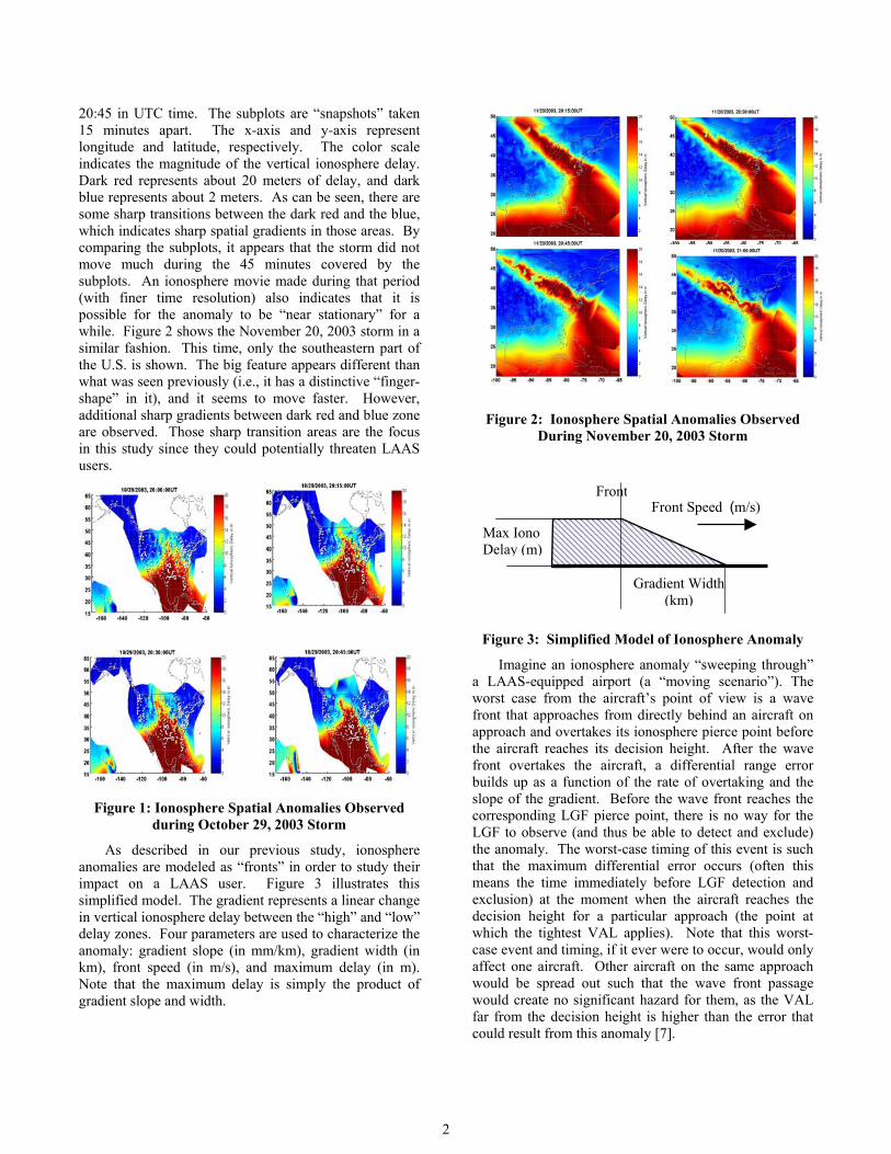
20:45 in UTC time. The subplots are “snapshots” taken 15 minutes apart. The x-axis and y-axis represent longitude and latitude, respectively. The color scale indicates the magnitude of the vertical ionosphere delay. Dark red represents about 20 meters of delay, and dark blue represents about 2 meters. As can be seen, there are some sharp transitions between the dark red and the blue, which indicates sharp spatial gradients in those areas. By comparing the subplots, it appears that the storm did not move much during the 45 minutes covered by the subplots. An ionosphere movie made during that period (with finer time resolution) also indicates that it is possible for the anomaly to be “near stationary” for a while. Figure 2 shows the November 20, 2003 storm in a similar fashion. This time, only the southeastern part of the U.S. is shown. The big feature appears different than what was seen previously (i.e., it has a distinctive “finger-shape” in it), and it seems to move faster. However, additional sharp gradients between dark red and blue zone are observed. Those sharp transition areas are the focus in this study since they could potentially threaten LAAS users.
Figure 1: Ionosphere Spatial Anomalies Observed during October 29, 2003 Storm
As described in our previous study, ionosphere anomalies are modeled as “fronts” in order to study their impact on a LAAS user. Figure 3 illustrates this simplified model. The gradient represents a linear change in vertical ionosphere delay between the “high” and “low” delay zones. Four parameters are used to characterize the anomaly: gradient slope (in mm/km), gradient width (in km), front speed (in m/s), and maximum delay (in m). Note that the maximum delay is simply the product of gradient slope and width.
Figure 2: Ionosphere Spatial Anomalies Observed
During November 20, 2003 Storm
Figure 3: Simplified Model of Ionosphere Anomaly
Imagine an ionosphere anomaly “sweeping through” a LAAS-equipped airport (a “moving scenario”). The worst case from the aircraft’s point of view is a wave front that approaches from directly behind an aircraft on approach and overtakes its ionosphere pierce point before the aircraft reaches its decision height. After the wave front overtakes the aircraft, a differential range error builds up as a function of the rate of overtaking and the slope of the gradient. Before the wave front reaches the corresponding LGF pierce point, there is no way for the LGF to observe (and thus be able to detect and exclude) the anomaly. The worst-case timing of this event is such that the maximum differential error occurs (often this means the time immediately before LGF detection and exclusion) at the moment when the aircraft reaches the decision height for a particular approach (the point at which the tightest VAL applies). Note that this worst-case event and timing, if it ever were to occur, would only affect one aircraft. Other aircraft on the same approach would be spread out such that the wave front passage would create no significant hazard for them, as the VAL far from the decision height is higher than the error that could result from this anomaly [7].
Max Iono Delay (m)
Front Speed (m/s)
Gradient Width (km)
Front
3
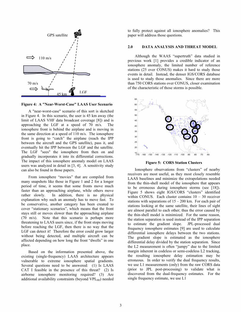
Figure 4: A "Near-Worst-Case" LAAS User Scenario
A "near-worst-case" scenario of this sort is sketched in Figure 4. In this scenario, the user is 45 km away (the limit of LAAS VHF data broadcast coverage [8]) and is approaching the LGF at a speed of 70 m/s. The ionosphere front is behind the airplane and is moving in the same direction at a speed of 110 m/s. The ionosphere front is going to “catch” the airplane (reach the IPP between the aircraft and the GPS satellite), pass it, and eventually hit the IPP between the LGF and the satellite. The LGF "sees" the ionosphere from then on and gradually incorporates it into its differential corrections. The impact of this ionosphere anomaly model on LAAS users was analyzed in detail in [3, 4]. A sensitivity study can also be found in those papers.
From ionosphere “movies” that are compiled from many snapshots like those in Figure 1 and 2 for a longer period of time, it seems that some fronts move much faster than an approaching airplane, while others move rather slowly. In addition, there is no physical explanation why such an anomaly has to move fast. To be conservative, another category has been created to cover “stationary scenarios”, which means that the front stays still or moves slower than the approaching airplane (70 m/s). Note that this scenario is perhaps more threatening to LAAS users since, if the front stops moving before reaching the LGF, then there is no way that the LGF can detect it! Therefore the error could grow larger without being detected, and multiple aircraft can be affected depending on how long the front “dwells” in one place.
Based on the information presented above, the existing (single-frequency) LAAS architecture appears vulnerable to extreme ionosphere spatial gradients. Several questions need to be answered: (1) Is LAAS CAT I feasible in the presence of this threat? (2) Is airborne ionosphere monitoring required? (3) Are additional availability constraints (beyond VPLH0) needed
to fully protect against all ionosphere anomalies? This paper will address those questions.
2.0 DATA ANALYSIS AND THREAT MODEL
Although the WAAS “supertruth” data studied in previous work [1] provides a credible indicator of an ionosphere anomaly, the limited number of reference stations (25 over CONUS) makes it hard to study those events in detail. Instead, the denser IGS/CORS database is used to study those anomalies. Since there are more than 750 CORS stations over CONUS, closer examination of the characteristic of those storms is possible.
Figure 5: CORS Station Clusters
Ionosphere observations from “clusters” of nearby receivers are most useful, as they most closely resemble LAAS baselines and minimize the extrapolations needed from the thin-shell model of the ionosphere that appears to be erroneous during ionosphere storms (see [18]). Figure 5 shows eight IGS/CORS “clusters” identified within CONUS. Each cluster contains 10 – 30 receiver stations with separations of 15 – 200 km. For each pair of stations looking at the same satellite, their lines of sight are almost parallel to each other; thus the error caused by the thin-shell model is minimized. For the same reason, the station separation is used instead of the IPP separation to estimate the gradient slope. JPL-processed dual frequency ionosphere estimates [9] are used to calculate differential ionosphere delays between the two stations. The gradient slope is estimated as the ionosphere differential delay divided by the station separation. Since the L2 measurement is often “jumpy” due to the limited margin inherent in codeless or semi-codeless L2 tracking, the resulting ionosphere delay estimation may be erroneous. In order to verify the dual frequency results, we use L1 measurements (only) from the raw CORS data (prior to JPL post-processing) to validate what is discovered from the dual-frequency estimates. For the single frequency estimate, we use L1
110 m/s
70 m/s
45 km LGF
GPS satellite
-170 -160 -150 -140 -130 -120 -110 -100 -90 -80 -70 -6015
20
25
30
35
40
45
50
55
60
65
4
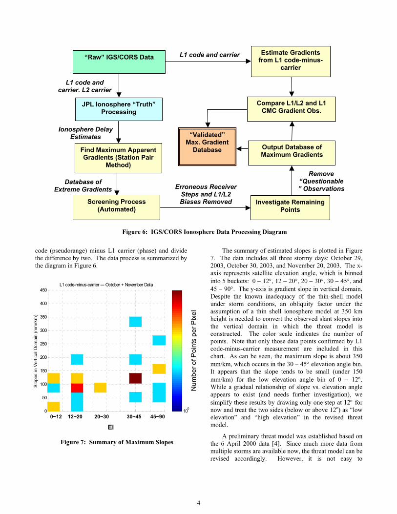
Figure 6: IGS/CORS Ionosphere Data Processing Diagram
code (pseudorange) minus L1 carrier (phase) and divide the difference by two. The data process is summarized by the diagram in Figure 6.
Figure 7: Summary of Maximum Slopes
The summary of estimated slopes is plotted in Figure 7. The data includes all three stormy days: October 29, 2003, October 30, 2003, and November 20, 2003. The x-axis represents satellite elevation angle, which is binned into 5 buckets: 0 − 12°, 12 − 20°, 20 − 30°, 30 − 45°, and 45 − 90°. The y-axis is gradient slope in vertical domain. Despite the known inadequacy of the thin-shell model under storm conditions, an obliquity factor under the assumption of a thin shell ionosphere model at 350 km height is needed to convert the observed slant slopes into the vertical domain in which the threat model is constructed. The color scale indicates the number of points. Note that only those data points confirmed by L1 code-minus-carrier measurement are included in this chart. As can be seen, the maximum slope is about 350 mm/km, which occurs in the 30 – 45° elevation angle bin. It appears that the slope tends to be small (under 150 mm/km) for the low elevation angle bin of 0 − 12°. While a gradual relationship of slope vs. elevation angle appears to exist (and needs further investigation), we simplify these results by drawing only one step at 12° for now and treat the two sides (below or above 12o) as “low elevation” and “high elevation” in the revised threat model.
A preliminary threat model was established based on the 6 April 2000 data [4]. Since much more data from multiple storms are available now, the threat model can be revised accordingly. However, it is not easy to
0
50
100
150
200
250
300
350
400
450L1 code-minus-carrier --- October + November Data
Slo
pes
in V
ertic
al D
omai
n (m
m/k
m)
Num
ber o
f Poi
nts
per P
ixel
100
0~12 45~9030~45 20~30 12~20
El
L1 code and carrier
L1 code and carrier, L2 carrier
“Raw” IGS/CORS Data
JPL Ionosphere “Truth” Processing
Ionosphere Delay Estimates
Find Maximum Apparent Gradients (Station Pair
Method)
Screening Process (Automated)
Database of Extreme Gradients Erroneous Receiver
Steps and L1/L2 Biases Removed Investigate Remaining
Points
Remove “Questionable” Observations
Estimate Gradients from L1 code-minus-
carrier
Output Database of Maximum Gradients
Compare L1/L2 and L1 CMC Gradient Obs.
“Validated” Max. Gradient
Database
5
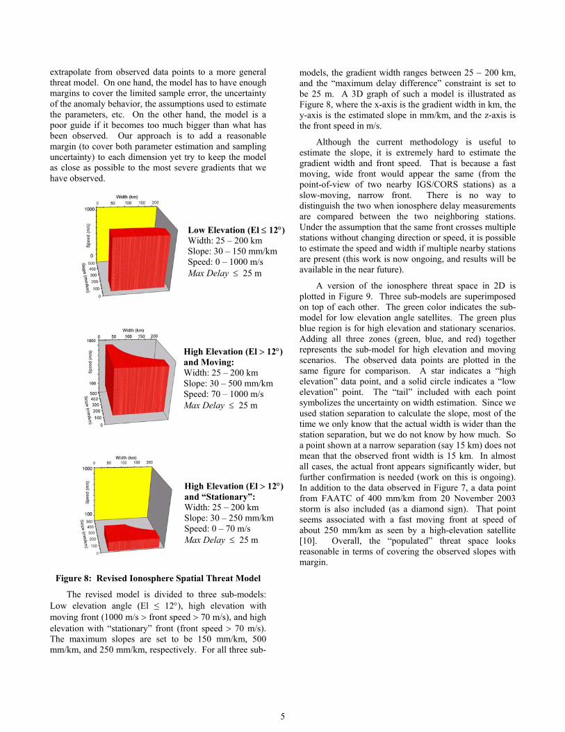
extrapolate from observed data points to a more general threat model. On one hand, the model has to have enough margins to cover the limited sample error, the uncertainty of the anomaly behavior, the assumptions used to estimate the parameters, etc. On the other hand, the model is a poor guide if it becomes too much bigger than what has been observed. Our approach is to add a reasonable margin (to cover both parameter estimation and sampling uncertainty) to each dimension yet try to keep the model as close as possible to the most severe gradients that we have observed.
Figure 8: Revised Ionosphere Spatial Threat Model
The revised model is divided to three sub-models: Low elevation angle (El ≤ 12°), high elevation with moving front (1000 m/s > front speed > 70 m/s), and high elevation with “stationary” front (front speed > 70 m/s). The maximum slopes are set to be 150 mm/km, 500 mm/km, and 250 mm/km, respectively. For all three sub-
models, the gradient width ranges between 25 − 200 km, and the “maximum delay difference” constraint is set to be 25 m. A 3D graph of such a model is illustrated as Figure 8, where the x-axis is the gradient width in km, the y-axis is the estimated slope in mm/km, and the z-axis is the front speed in m/s.
Although the current methodology is useful to estimate the slope, it is extremely hard to estimate the gradient width and front speed. That is because a fast moving, wide front would appear the same (from the point-of-view of two nearby IGS/CORS stations) as a slow-moving, narrow front. There is no way to distinguish the two when ionosphere delay measurements are compared between the two neighboring stations. Under the assumption that the same front crosses multiple stations without changing direction or speed, it is possible to estimate the speed and width if multiple nearby stations are present (this work is now ongoing, and results will be available in the near future).
A version of the ionosphere threat space in 2D is plotted in Figure 9. Three sub-models are superimposed on top of each other. The green color indicates the sub-model for low elevation angle satellites. The green plus blue region is for high elevation and stationary scenarios. Adding all three zones (green, blue, and red) together represents the sub-model for high elevation and moving scenarios. The observed data points are plotted in the same figure for comparison. A star indicates a “high elevation” data point, and a solid circle indicates a “low elevation” point. The “tail” included with each point symbolizes the uncertainty on width estimation. Since we used station separation to calculate the slope, most of the time we only know that the actual width is wider than the station separation, but we do not know by how much. So a point shown at a narrow separation (say 15 km) does not mean that the observed front width is 15 km. In almost all cases, the actual front appears significantly wider, but further confirmation is needed (work on this is ongoing). In addition to the data observed in Figure 7, a data point from FAATC of 400 mm/km from 20 November 2003 storm is also included (as a diamond sign). That point seems associated with a fast moving front at speed of about 250 mm/km as seen by a high-elevation satellite [10]. Overall, the “populated” threat space looks reasonable in terms of covering the observed slopes with margin.
Low Elevation (El ≤ 12°)Width: 25 – 200 km Slope: 30 – 150 mm/km Speed: 0 – 1000 m/s Max Delay ≤ 25 m
High Elevation (El > 12°) and Moving: Width: 25 – 200 km Slope: 30 – 500 mm/km Speed: 70 – 1000 m/s Max Delay ≤ 25 m
High Elevation (El > 12°) and “Stationary”: Width: 25 – 200 km Slope: 30 – 250 mm/km Speed: 0 – 70 m/s Max Delay ≤ 25 m

6
0 20 40 60 80 100 120 140 160 180 200 2200
50
100
150
200
250
300
350
400
450
500
550Revised Threat Models in 2D-View
Ionosphere Front W idth (km)
Iono
sphe
re F
ront
Slo
pe (m
m/k
m)
High Elevation + MovingHigh Elevation + StationaryLow Elevation
Figure 9: Two-Dimension Threat Space and
Observed Anomalies
3.0 THREAT ASSESSMENT
3.1 Assumptions on LGF and Airborne Monitors
In order to assess the threat of ionosphere spatial anomalies to a LAAS user, some assumptions have to be made on what kinds of monitors are employed and how those monitors perform against the threat. We used Stanford Integrity Monitoring Testbed (IMT), which is a prototype of LGF, to obtain approximate times-to-detect for various monitors. A detailed description of IMT design and validation testing can be found in [11, 12].
0.005 0.01 0.015 0.02 0.025 0.03 0.035 0.04 0.045 0.050
20
40
60
80
100
120
140
160
180
200
Ionospheric Rate (m/s)
Tim
e-to
-det
ect (
s)
Simplified Time-to-detect vs Ionospheric Rate
by LGFby Airborne
GMA Only
MQM
CUSUM
Figure 10: Time-to-detect vs. Ionosphere Delay Rate
of Change (from Stanford IMT Failure Testing)
Since each IMT monitor was designed to target different potential failure modes in LGF measurements, their times-to-detect vary with the apparent ionospheric delay rate-of-change as well as the satellite elevation angle. Generally, Measurement Quality Monitoring
(MQM, a function designed to detect sudden jumps or rapid acceleration in pseudorange and carrier phase measurements) is the fastest when the apparent ionospheric rate is above a certain level (e.g., greater than 0.02 m/s for a high-elevation-angle satellite), and the Cumulative Sum (CUSUM) code-carrier divergence monitor is the best when the ionosphere rate is lower than this but still anomalous (e.g., between 0.01 and 0.02 m/s) [13]. Based on IMT test results with injected failures, the overall time-to-detect by the LGF is shown as the blue line (circle points) in Figure 10. It is assumed that no monitor detects ionosphere events with apparent ionosphere delay rates-of-change at the LGF lower than 0.01 m/s (this is likely required to meet the LGF continuity sub-allocation during non-hazardous ionosphere storms). Note that these test results may be strongly associated with factors unique to the Stanford IMT such as siting, antenna type, etc. Thus, the values used here may need to be adjusted to suit a different LGF system design.
The only way to obtain and validate the performance of an airborne monitor is through GPS receiver flight-testing, as Boeing has been doing [14]. Before this data is available in quantity, we assume that the aircraft is using a Geometric Moving Averaging (GMA) code carrier divergence monitor, and its performance is equivalent to a ground-based GMA monitor with time constant of 200 s. The time-to-detect of such a monitor is also plotted in Figure 10 as the red curve (asterisk points). Clearly, it is much slower than the LGF monitors, and we hope that there is room for improvement.
3.2 Moving Wave Front Scenarios
As illustrated in Figure 4, if an ionosphere front is near a LAAS-equipped airport, a user may suffer an ionosphere delay that is different then what the LGF sees. The magnitude of the resulting differential error depends on the ionosphere front parameters (slope, width, and speed), the relative position between the front and the airplane, and the satellite geometry. For the purpose of assessing the maximum differential user error, we investigated some “worst-case geometries”, i.e., 22-of-24 satellites constellation with VPLH0 between 9.95 m to 10 m. (Those geometries with VPLH0 greater than 10 m would be screened out as “unavailable” and therefore are not included in this simulation.) For each ionosphere front permutation (combined slope, width, and speed), we simulated all the possible relative positions between the airplane and the LGF, for all selected geometries, and found the maximum error for that permutation.
7
0100
200300
400500
050
100
150200
0
10
20
30
40
50
60
Iono. Front Slope (mm/km)
Max Error vs Front Parameters, Revised Model, Worst 22SVs at New York, No Monitoring
Iono. Front Width (km)
Max
Ver
tical
Erro
r (m
)
Speed = 100 m/s
Figure 11: Moving Front with a Speed of 100 m/s
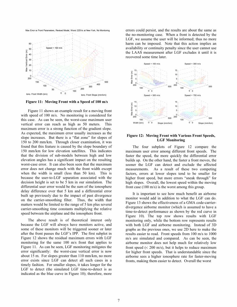
Figure 11 shows an example result for a moving front with speed of 100 m/s. No monitoring is considered for this case. As can be seen, the worst-case maximum user vertical error can reach as high as 50 meters. This maximum error is a strong function of the gradient slope. As expected, the maximum error usually increases as the slope increases. But there is a “flat zone” for slopes of 150 to 200 mm/km. Through closer examination, it was found that this feature is caused by the slope boundary of 150 mm/km for low elevation satellites. This indicates that the division of sub-models between high and low elevation angles has a significant impact on the resulting worst-case error. It can also been seen that the maximum error does not change much with the front width except when the width is small (less than 50 km). This is because the user-to-LGF separation associated with the decision height is set to be 5 km in our simulation. The differential user error would be the sum of the ionosphere delay difference over that 5 km and a differential error built up previously due to the impact of past divergence on the carrier-smoothing filter. Thus, the width that matters would be limited to the range of 5 km plus several carrier-smoothing time constants multiplying the relative speed between the airplane and the ionosphere front.
The above result is of theoretical interest only because the LGF will always have monitors active, and some of these monitors will be triggered sooner or later after the front passes the LGF’s IPP. The first subplot in Figure 12 shows the residual maximum errors with LGF monitoring for the same 100 m/s front that applies to Figure 11. As can be seen, LGF monitoring mitigates the error significantly: the worst-case vertical error is now about 15 m. For slopes greater than 110 mm/km, no more error exists since LGF can detect all such cases in a timely fashion. For smaller slopes, it takes longer for the LGF to detect (the simulated LGF time-to-detect is as indicated as the blue curve in Figure 10); therefore, more
errors could persist, and the results are about the same as the no-monitoring case. When a front is detected by the LGF, we assume the user will be informed; thus no more harm can be imposed. Note that this action implies an availability or continuity penalty since the user cannot use the LAAS measurement after LGF excludes it until it is recovered some time later.
0
500
0100
2000
5
10
15
Speed = 100 m/s
Max
Erro
r (m
)
0
500
0100
2000
5
10
15
Speed = 300 m/s
0
500
0100
2000
5
10
15
Slope (mm/km)
Speed = 500 m/s
Width (km)
Max
Erro
r (m
)
0
500
0100
2000
5
10
15
Slope (mm/km)
Speed = 700 m/s
Figure 12: Moving Front with Various Front Speeds, LGF Monitoring
The four subplots of Figure 12 compare the maximum user error among different front speeds. The faster the speed, the more quickly the differential error builds up. On the other hand, the faster a front moves, the sooner the LGF can detect and exclude the affected measurements. As a result of these two competing factors, errors at lower slopes tend to be smaller for higher front speed, but more errors “sneak through” for high slopes. Overall, the lowest speed within the moving front case (100 m/s) is the worst among this group.
It is important to see how much benefit an airborne monitor would add in addition to what the LGF can do. Figure 13 shows the effectiveness of a GMA code-carrier-divergence airborne monitor (which is assumed to have a time-to-detect performance as shown by the red curve in Figure 10). The top row shows results with LGF monitoring only, while the bottom row represents results with both LGF and airborne monitoring. Instead of 3D graphs as the previous ones, we use 2D here to make the results easier to read. Front speeds from 100 m/s to 1000 m/s are simulated and compared. As can be seen, the airborne monitor does not help much for relatively low front speed (< 200 m/s), but it helps to reduce maximum for higher front speeds. That is understandable since the airborne sees a higher ionosphere rate for faster-moving fronts, making them easier to detect. Overall the worst

8
0 100 2000
5
10
15100 m/s
Max
Erro
r w/ L
GF
(m)
0 100 2000
5
10
15300 m/s
0 100 2000
5
10
15500 m/s
0 100 2000
5
10
15700 m/s
0 100 2000
5
10
15900 m/s
0 100 2000
5
10
15
Max
Erro
r w/ L
GF
& A
ir (m
)
W idth (km)
100 m/s
0 100 2000
5
10
15
Width (km)
300 m/s
0 100 2000
5
10
15500 m/s
Width (km)0 100 200
0
5
10
15700 m/s
Width (km)0 100 200
0
5
10
15900 m/s
Width (km) Figure 13: Comparison between LGF Monitoring vs.
LGF and Airborne Monitoring
case is still at low speed (100 m/s), and the residual error is about the same (15 m). For moving scenarios, it appears that the effectiveness of an airborne monitor is significant, but not dramatic.
3.3 Stationary Scenarios
As shown in previous work [5], if an ionosphere front slows down its motion or even becomes near-stationary, it can be more threatening to a LAAS user because the LGF may never be able to detect it. Based on the threat model illustrated in Figure 8, we simulated the worst cases for stationary scenarios, and the results are shown in Figure 14. The same “worst” geometries are used as for the moving scenarios. Note that the threat model has lower ceiling of slope for stationary cases (250 mm/km) than for moving fronts (500 mm/km). We assume the LGF can detect the anomaly if the front is located such that LGF sees the ramp or the elevated part of the ionosphere. In other words, as long as the tip of the front impacts the line of sight of at least one LGF reference receiver, then the anomaly will be detected and removed. This is probably a bit optimistic since it may not always be the case if the front moves in (or forms) very slowly before becoming stationary. But if the LGF has three or four reference receivers with separated antennas (see [15]), the front will likely be detected as it moves in. For airborne monitoring, we assume the same GMA monitor with a time constant of 200 s (the same as in Section 3.2).
0100
2000
100200
0
10
20
30
No Monitoring
Ver
tical
Erro
r (m
)
0100
2000
100200
0
10
20
30
LGF Monitoring
0100
2000
1002000
10
20
30
Slope (mm/km)
Airborne Monitoring
Width (km)
Ver
tical
Erro
r (m
)
0100
2000
100200
0
10
20
30
LGF & Airborne Monitoring
Figure 14: Maximum Errors for Stationary Scenarios
Figure 14 compares the maximum error under LGF, airborne, and LGF-plus-airborne monitoring conditions. The worst-case vertical position errors are 26, 23, 22, and 21 m respectively – all of these are larger than the worst case moving fronts from Section 3.2. Similar to the moving scenarios, the maximum error is a strong function of slope, has a “flat zone” due to the slope boundary of 150 mm/km for low elevation satellites, and is not sensitive to front width. With LGF (the upper right subplot) or airborne (the lower left subplot) monitoring alone, the maximum error is reduced a little bit but the overall picture looks about the same. Only when both LGF and airborne monitors are in place (the lower right subplot) do they effectively mitigate any slope greater than 140 mm/km; thus the worst-case errors become zero for that region (nominal LAAS error distributions apply for the satellites not affected by the anomaly). Although this result may appear to be non-intuitive, it actually makes sense after a close examination. The reason is that LGF and airborne monitors mitigate ionosphere front at different wave front locations along the approach path. If only some of these locations are protected, the residual error is about the same as if there were no monitoring at all. Only when both LGF and airborne monitors are in place are all potentially hazardous locations detected.
There is also a clear reason for the detectable “cutoff” point of 140 mm/km. Note that the limit of both LGF and airborne monitors is at 0.01 m/s (see Figure 10). For a stationary front, this directly translates into a spatial gradient of 143 mm/km:
Spatial Slope = Ionosphere Rate / Relative Speed
Since the relative speed is equal to the airplane speed of 70 m/s when the front is stationary, the detectable slope associated with the detectable ionosphere rate becomes:
Spatial Slope = 0.01 / 70 = 1.43 × 10⁻⁴ m/m = 143 mm/km
9
This result sets the fundamental limit of the effectiveness of monitors that observe time rates of change. As noted before, the one-sigma value of ionosphere spatial gradients under nominal conditions is about 2 − 5 mm/km (1σ). It is impossible to set the threshold much lower than 0.01 m/s otherwise it will alert too often under nominal conditions and therefore harm continuity and availability. However, if monitors exist that can observe the ionosphere spatial difference directly (instead of inferring it from a time rate of change), it may be possible to make this limiting slope lower.
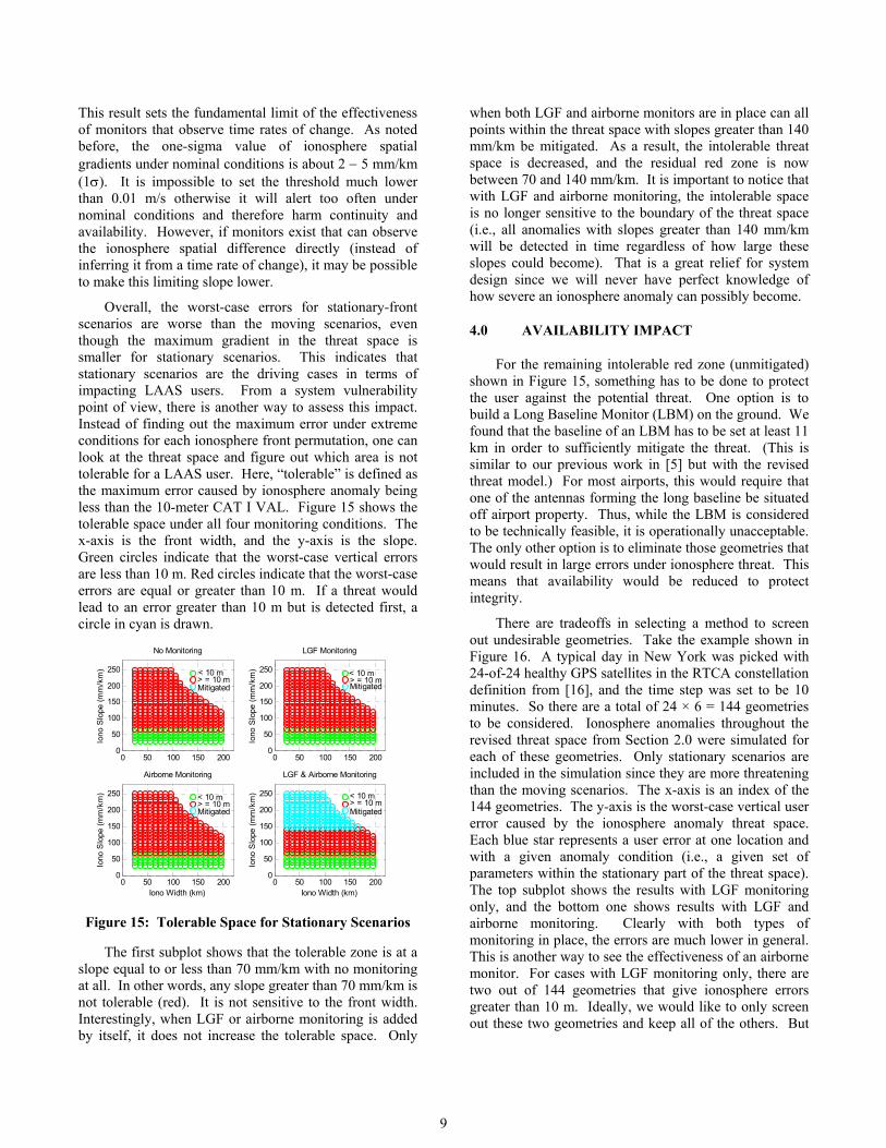
Overall, the worst-case errors for stationary-front scenarios are worse than the moving scenarios, even though the maximum gradient in the threat space is smaller for stationary scenarios. This indicates that stationary scenarios are the driving cases in terms of impacting LAAS users. From a system vulnerability point of view, there is another way to assess this impact. Instead of finding out the maximum error under extreme conditions for each ionosphere front permutation, one can look at the threat space and figure out which area is not tolerable for a LAAS user. Here, “tolerable” is defined as the maximum error caused by ionosphere anomaly being less than the 10-meter CAT I VAL. Figure 15 shows the tolerable space under all four monitoring conditions. The x-axis is the front width, and the y-axis is the slope. Green circles indicate that the worst-case vertical errors are less than 10 m. Red circles indicate that the worst-case errors are equal or greater than 10 m. If a threat would lead to an error greater than 10 m but is detected first, a circle in cyan is drawn.
0 50 100 150 2000
50
100
150
200
250
Iono
Slo
pe (m
m/k
m)
No Monitoring
0 50 100 150 2000
50
100
150
200
250
Iono
Slo
pe (m
m/k
m)
LGF Monitoring
0 50 100 150 2000
50
100
150
200
250
Iono Width (km)
Iono
Slo
pe (m
m/k
m)
Airborne Monitoring
0 50 100 150 2000
50
100
150
200
250
Iono Width (km)
Iono
Slo
pe (m
m/k
m)
LGF & Airborne Monitoring
< 10 m > = 10 m Mitigated Mitigated
< 10 m > = 10 m
< 10 m > = 10 m Mitigated
< 10 m > = 10 m Mitigated
Figure 15: Tolerable Space for Stationary Scenarios
The first subplot shows that the tolerable zone is at a
slope equal to or less than 70 mm/km with no monitoring at all. In other words, any slope greater than 70 mm/km is not tolerable (red). It is not sensitive to the front width. Interestingly, when LGF or airborne monitoring is added by itself, it does not increase the tolerable space. Only
when both LGF and airborne monitors are in place can all points within the threat space with slopes greater than 140 mm/km be mitigated. As a result, the intolerable threat space is decreased, and the residual red zone is now between 70 and 140 mm/km. It is important to notice that with LGF and airborne monitoring, the intolerable space is no longer sensitive to the boundary of the threat space (i.e., all anomalies with slopes greater than 140 mm/km will be detected in time regardless of how large these slopes could become). That is a great relief for system design since we will never have perfect knowledge of how severe an ionosphere anomaly can possibly become.
4.0 AVAILABILITY IMPACT
For the remaining intolerable red zone (unmitigated) shown in Figure 15, something has to be done to protect the user against the potential threat. One option is to build a Long Baseline Monitor (LBM) on the ground. We found that the baseline of an LBM has to be set at least 11 km in order to sufficiently mitigate the threat. (This is similar to our previous work in [5] but with the revised threat model.) For most airports, this would require that one of the antennas forming the long baseline be situated off airport property. Thus, while the LBM is considered to be technically feasible, it is operationally unacceptable. The only other option is to eliminate those geometries that would result in large errors under ionosphere threat. This means that availability would be reduced to protect integrity.
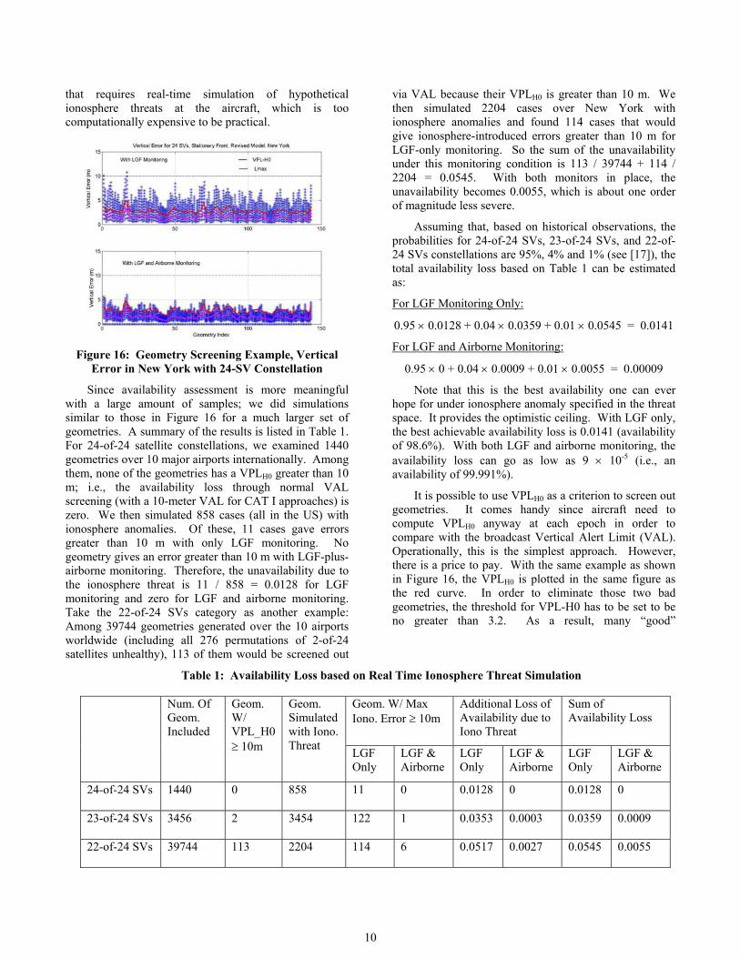
There are tradeoffs in selecting a method to screen out undesirable geometries. Take the example shown in Figure 16. A typical day in New York was picked with 24-of-24 healthy GPS satellites in the RTCA constellation definition from [16], and the time step was set to be 10 minutes. So there are a total of 24 × 6 = 144 geometries to be considered. Ionosphere anomalies throughout the revised threat space from Section 2.0 were simulated for each of these geometries. Only stationary scenarios are included in the simulation since they are more threatening than the moving scenarios. The x-axis is an index of the 144 geometries. The y-axis is the worst-case vertical user error caused by the ionosphere anomaly threat space. Each blue star represents a user error at one location and with a given anomaly condition (i.e., a given set of parameters within the stationary part of the threat space). The top subplot shows the results with LGF monitoring only, and the bottom one shows results with LGF and airborne monitoring. Clearly with both types of monitoring in place, the errors are much lower in general. This is another way to see the effectiveness of an airborne monitor. For cases with LGF monitoring only, there are two out of 144 geometries that give ionosphere errors greater than 10 m. Ideally, we would like to only screen out these two geometries and keep all of the others. But
10
that requires real-time simulation of hypothetical ionosphere threats at the aircraft, which is too computationally expensive to be practical.
Figure 16: Geometry Screening Example, Vertical
Error in New York with 24-SV Constellation
Since availability assessment is more meaningful with a large amount of samples; we did simulations similar to those in Figure 16 for a much larger set of geometries. A summary of the results is listed in Table 1. For 24-of-24 satellite constellations, we examined 1440 geometries over 10 major airports internationally. Among them, none of the geometries has a VPLH0 greater than 10 m; i.e., the availability loss through normal VAL screening (with a 10-meter VAL for CAT I approaches) is zero. We then simulated 858 cases (all in the US) with ionosphere anomalies. Of these, 11 cases gave errors greater than 10 m with only LGF monitoring. No geometry gives an error greater than 10 m with LGF-plus-airborne monitoring. Therefore, the unavailability due to the ionosphere threat is 11 / 858 = 0.0128 for LGF monitoring and zero for LGF and airborne monitoring. Take the 22-of-24 SVs category as another example: Among 39744 geometries generated over the 10 airports worldwide (including all 276 permutations of 2-of-24 satellites unhealthy), 113 of them would be screened out
via VAL because their VPLH0 is greater than 10 m. We then simulated 2204 cases over New York with ionosphere anomalies and found 114 cases that would give ionosphere-introduced errors greater than 10 m for LGF-only monitoring. So the sum of the unavailability under this monitoring condition is 113 / 39744 + 114 / 2204 = 0.0545. With both monitors in place, the unavailability becomes 0.0055, which is about one order of magnitude less severe.
Assuming that, based on historical observations, the probabilities for 24-of-24 SVs, 23-of-24 SVs, and 22-of-24 SVs constellations are 95%, 4% and 1% (see [17]), the total availability loss based on Table 1 can be estimated as:
For LGF Monitoring Only:
0.95 × 0.0128 + 0.04 × 0.0359 + 0.01 × 0.0545 = 0.0141
For LGF and Airborne Monitoring:
0.95 × 0 + 0.04 × 0.0009 + 0.01 × 0.0055 = 0.00009
Note that this is the best availability one can ever hope for under ionosphere anomaly specified in the threat space. It provides the optimistic ceiling. With LGF only, the best achievable availability loss is 0.0141 (availability of 98.6%). With both LGF and airborne monitoring, the availability loss can go as low as 9 × 10⁻⁵ (i.e., an availability of 99.991%).
It is possible to use VPLH0 as a criterion to screen out geometries. It comes handy since aircraft need to compute VPLH0 anyway at each epoch in order to compare with the broadcast Vertical Alert Limit (VAL). Operationally, this is the simplest approach. However, there is a price to pay. With the same example as shown in Figure 16, the VPLH0 is plotted in the same figure as the red curve. In order to eliminate those two bad geometries, the threshold for VPL-H0 has to be set to be no greater than 3.2. As a result, many “good”
Table 1: Availability Loss based on Real Time Ionosphere Threat Simulation
Geom. W/ Max Iono. Error ≥ 10m
Additional Loss of Availability due to Iono Threat
Sum of Availability Loss
Num. Of Geom. Included
Geom. W/ VPL_H0 ≥ 10m
Geom. Simulated with Iono. Threat LGF
Only LGF & Airborne
LGF Only
LGF & Airborne
LGF Only
LGF & Airborne
24-of-24 SVs 1440 0 858 11 0 0.0128 0 0.0128 0
23-of-24 SVs 3456 2 3454 122 1 0.0353 0.0003 0.0359 0.0009
22-of-24 SVs 39744 113 2204 114 6 0.0517 0.0027 0.0545 0.0055
11
geometries have to be thrown out in addition to the ones that must be thrown out based on ionosphere simulations. That is a significant additional price to pay in terms of additional availability loss.
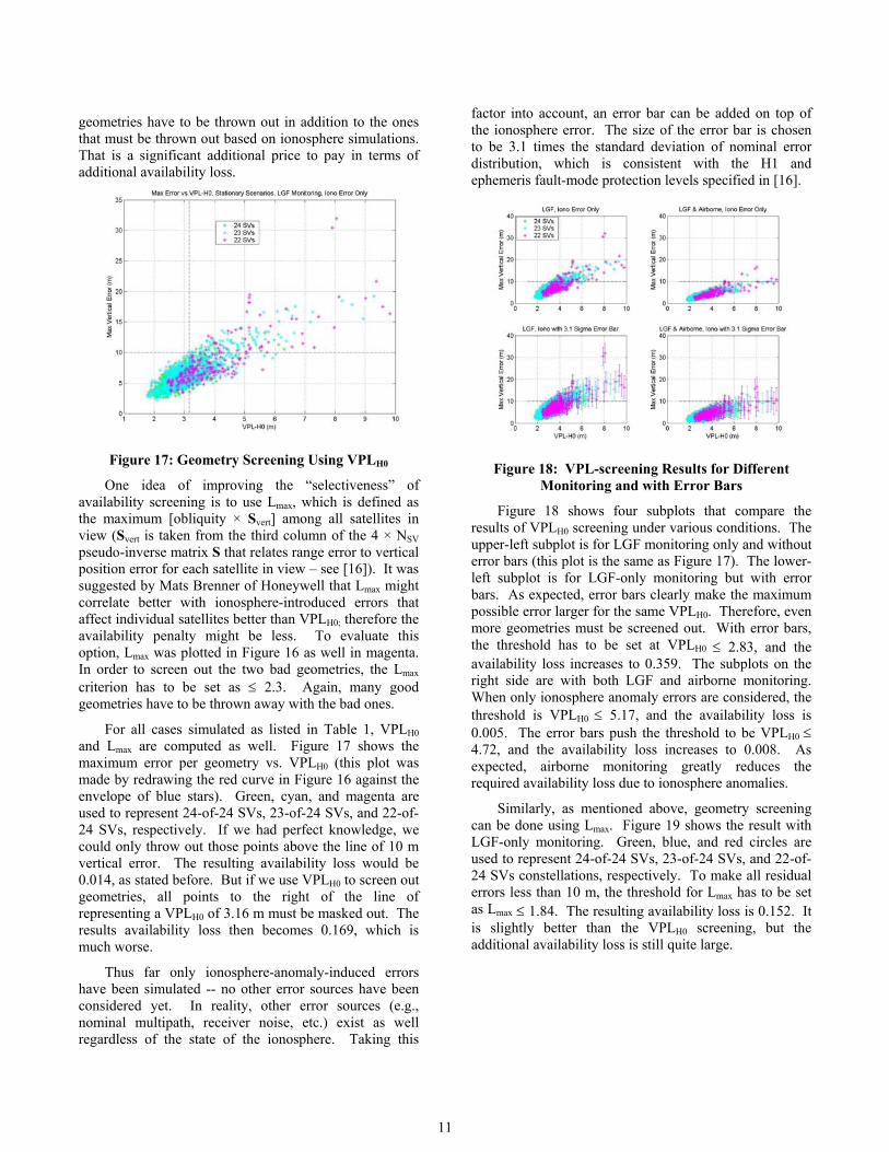
Figure 17: Geometry Screening Using VPLH0
One idea of improving the “selectiveness” of availability screening is to use Lmax, which is defined as the maximum [obliquity × Svert] among all satellites in view (Svert is taken from the third column of the 4 × NSV pseudo-inverse matrix S that relates range error to vertical position error for each satellite in view – see [16]). It was suggested by Mats Brenner of Honeywell that Lmax might correlate better with ionosphere-introduced errors that affect individual satellites better than VPLH0; therefore the availability penalty might be less. To evaluate this option, Lmax was plotted in Figure 16 as well in magenta. In order to screen out the two bad geometries, the Lmax criterion has to be set as ≤ 2.3. Again, many good geometries have to be thrown away with the bad ones.
For all cases simulated as listed in Table 1, VPLH0 and Lmax are computed as well. Figure 17 shows the maximum error per geometry vs. VPLH0 (this plot was made by redrawing the red curve in Figure 16 against the envelope of blue stars). Green, cyan, and magenta are used to represent 24-of-24 SVs, 23-of-24 SVs, and 22-of-24 SVs, respectively. If we had perfect knowledge, we could only throw out those points above the line of 10 m vertical error. The resulting availability loss would be 0.014, as stated before. But if we use VPLH0 to screen out geometries, all points to the right of the line of representing a VPLH0 of 3.16 m must be masked out. The results availability loss then becomes 0.169, which is much worse.
Thus far only ionosphere-anomaly-induced errors have been simulated -- no other error sources have been considered yet. In reality, other error sources (e.g., nominal multipath, receiver noise, etc.) exist as well regardless of the state of the ionosphere. Taking this
factor into account, an error bar can be added on top of the ionosphere error. The size of the error bar is chosen to be 3.1 times the standard deviation of nominal error distribution, which is consistent with the H1 and ephemeris fault-mode protection levels specified in [16].
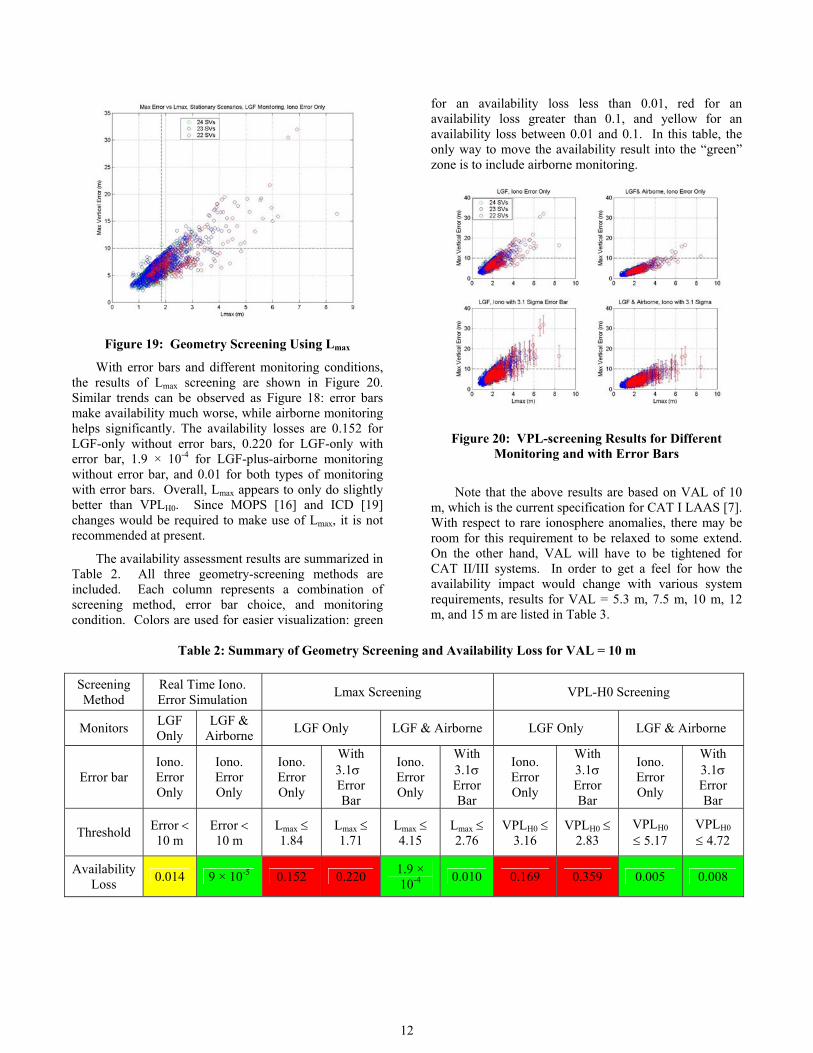
Figure 18: VPL-screening Results for Different
Monitoring and with Error Bars
Figure 18 shows four subplots that compare the results of VPLH0 screening under various conditions. The upper-left subplot is for LGF monitoring only and without error bars (this plot is the same as Figure 17). The lower-left subplot is for LGF-only monitoring but with error bars. As expected, error bars clearly make the maximum possible error larger for the same VPLH0. Therefore, even more geometries must be screened out. With error bars, the threshold has to be set at VPLH0 ≤ 2.83, and the availability loss increases to 0.359. The subplots on the right side are with both LGF and airborne monitoring. When only ionosphere anomaly errors are considered, the threshold is VPLH0 ≤ 5.17, and the availability loss is 0.005. The error bars push the threshold to be VPLH0 ≤ 4.72, and the availability loss increases to 0.008. As expected, airborne monitoring greatly reduces the required availability loss due to ionosphere anomalies.
Similarly, as mentioned above, geometry screening can be done using Lmax. Figure 19 shows the result with LGF-only monitoring. Green, blue, and red circles are used to represent 24-of-24 SVs, 23-of-24 SVs, and 22-of-24 SVs constellations, respectively. To make all residual errors less than 10 m, the threshold for Lmax has to be set as Lmax ≤ 1.84. The resulting availability loss is 0.152. It is slightly better than the VPLH0 screening, but the additional availability loss is still quite large.
12
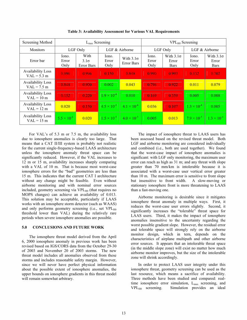
Figure 19: Geometry Screening Using Lmax
With error bars and different monitoring conditions, the results of Lmax screening are shown in Figure 20. Similar trends can be observed as Figure 18: error bars make availability much worse, while airborne monitoring helps significantly. The availability losses are 0.152 for LGF-only without error bars, 0.220 for LGF-only with error bar, 1.9 × 10⁻⁴ for LGF-plus-airborne monitoring without error bar, and 0.01 for both types of monitoring with error bars. Overall, Lmax appears to only do slightly better than VPLH0. Since MOPS [16] and ICD [19] changes would be required to make use of Lmax, it is not recommended at present.
The availability assessment results are summarized in Table 2. All three geometry-screening methods are included. Each column represents a combination of screening method, error bar choice, and monitoring condition. Colors are used for easier visualization: green
for an availability loss less than 0.01, red for an availability loss greater than 0.1, and yellow for an availability loss between 0.01 and 0.1. In this table, the only way to move the availability result into the “green” zone is to include airborne monitoring.
Figure 20: VPL-screening Results for Different Monitoring and with Error Bars
Note that the above results are based on VAL of 10 m, which is the current specification for CAT I LAAS [7]. With respect to rare ionosphere anomalies, there may be room for this requirement to be relaxed to some extend. On the other hand, VAL will have to be tightened for CAT II/III systems. In order to get a feel for how the availability impact would change with various system requirements, results for VAL = 5.3 m, 7.5 m, 10 m, 12 m, and 15 m are listed in Table 3.
Table 2: Summary of Geometry Screening and Availability Loss for VAL = 10 m
Screening Method
Real Time Iono. Error Simulation Lmax Screening VPL-H0 Screening
Monitors LGF Only
LGF & Airborne LGF Only LGF & Airborne LGF Only LGF & Airborne
Error bar Iono. Error Only
Iono. Error Only
Iono. Error Only
With 3.1σ Error Bar
Iono. Error Only
With 3.1σ Error Bar
Iono. Error Only
With 3.1σ Error Bar
Iono. Error Only
With 3.1σ Error Bar
Threshold Error < 10 m
Error < 10 m
Lmax ≤ 1.84
Lmax ≤ 1.71
Lmax ≤ 4.15
Lmax ≤ 2.76
VPLH0 ≤ 3.16
VPLH0 ≤ 2.83
VPLH0 ≤ 5.17
VPLH0 ≤ 4.72
Availability Loss 0.014 9 × 10⁻⁵ 0.152 0.220 1.9 ×
10-4 0.010 0.169 0.359 0.005 0.008
13
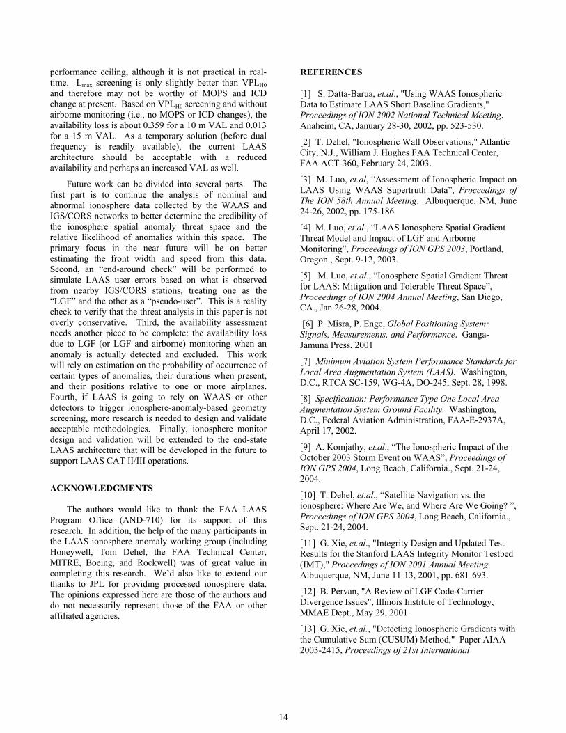
Table 3: Availability Assessment for Various VAL Requirements Screening Method Lmax Screening VPLH0 Screening
Monitors LGF Only LGF & Airborne LGF Only LGF & Airborne
Error bar Iono. Error Only
With 3.1σ
Error Bars
Iono. Error Only
With 3.1σ Error Bars
Iono. Error Only
With 3.1σ Error Bars
Iono. Error Only
With 3.1σ Error Bars
Availability Loss VAL = 5.3 m 0.996 0.996 0.150 0.848 0.990 0.993 0.132 0.702
Availability Loss VAL = 7.5 m 0.848 0.900 0.002 0.043 0.796 0.922 0.011 0.079
Availability Loss VAL = 10 m 0.152 0.220 1.9 × 10⁻⁴ 0.010 0.169 0.359 0.005 0.008
Availability Loss VAL = 12 m 0.020 0.150 4.5 × 10⁻⁵ 4.1 × 10⁻⁴ 0.036 0.107 1.3 × 10⁻⁴ 0.005
Availability Loss VAL = 15 m 5.5 × 10⁻⁴ 0.020 1.5 × 10⁻⁵ 4.0 × 10⁻⁵ 0.005 0.013 7.9 × 10⁻⁵ 1.3 × 10⁻⁴
For VAL’s of 5.3 m or 7.5 m, the availability loss due to ionosphere anomalies is clearly too large. That means that a CAT II/III system is probably not realistic for the current single-frequency-based LAAS architecture unless the ionosphere anomaly threat space can be significantly reduced. However, if the VAL increases to 12 m or 15 m, availability increases sharply comparing with a VAL of 10 m. That is because most worst-case ionosphere errors for the “bad” geometries are less than 15 m. This indicates that the current CAT I architecture without any change might be feasible. Even without airborne monitoring and with nominal error sources included, geometry screening via VPLH0 (that requires no MOPS changes) can achieve an availability of 0.013. This solution may be acceptable, particularly if LAAS works with an ionosphere storm detector (such as WAAS) and only performs geometry screening (i.e., set VPLH0 threshold lower than VAL) during the relatively rare periods when severe ionosphere anomalies are possible.
5.0 CONCLUSIONS AND FUTURE WORK
The ionosphere threat model derived from the April 6, 2000 ionosphere anomaly in previous work has been revised based on IGS/CORS data from the October 29-30 of 2003 and November 20 of 2003 storms. The new threat model includes all anomalies observed from these storms and includes reasonable safety margin. However, since we will never have perfect physical information about the possible extent of ionosphere anomalies, the upper bounds on ionosphere gradients in this threat model will remain somewhat arbitrary.
The impact of ionosphere threat to LAAS users has been assessed based on the revised threat model. Both LGF and airborne monitoring are considered individually and combined (i.e., both are used together). We found that the worst-case impact of ionosphere anomalies is significant: with LGF only monitoring, the maximum user error can reach as high as 31 m; and any threat with slope greater than 70 mm/km is intolerable because it is associated with a worst-case user vertical error greater than 10 m. The maximum error is sensitive to front slope but insensitive to front width. A slow-moving or stationary ionosphere front is more threatening to LAAS than a fast-moving one.
Airborne monitoring is desirable since it mitigates ionosphere threat anomaly in multiple ways. First, it reduces the worst-case user errors slightly. Second, it significantly increases the “tolerable” threat space for LAAS users. Third, it makes the impact of ionosphere anomalies insensitive to the uncertainty regarding the worst possible gradient slope. However, the residual error and tolerable space will strongly rely on the airborne monitor design, which in tern, depends on the characteristics of airplane multipath and other airborne error sources. It appears that an intolerable threat space (in the middle slope zone) will exist no matter how much airborne monitor improves, but the size of the intolerable zone will shrink accordingly.
In order to protect LAAS user integrity under this ionosphere threat, geometry screening can be used as the last resource, which means a sacrifice of availability. Three methods have been studied and compared: real-time ionosphere error simulation, Lmax screening, and VPLH0 screening. Simulation provides an ideal
14
performance ceiling, although it is not practical in real-time. Lmax screening is only slightly better than VPLH0 and therefore may not be worthy of MOPS and ICD change at present. Based on VPLH0 screening and without airborne monitoring (i.e., no MOPS or ICD changes), the availability loss is about 0.359 for a 10 m VAL and 0.013 for a 15 m VAL. As a temporary solution (before dual frequency is readily available), the current LAAS architecture should be acceptable with a reduced availability and perhaps an increased VAL as well.
Future work can be divided into several parts. The first part is to continue the analysis of nominal and abnormal ionosphere data collected by the WAAS and IGS/CORS networks to better determine the credibility of the ionosphere spatial anomaly threat space and the relative likelihood of anomalies within this space. The primary focus in the near future will be on better estimating the front width and speed from this data. Second, an “end-around check” will be performed to simulate LAAS user errors based on what is observed from nearby IGS/CORS stations, treating one as the “LGF” and the other as a “pseudo-user”. This is a reality check to verify that the threat analysis in this paper is not overly conservative. Third, the availability assessment needs another piece to be complete: the availability loss due to LGF (or LGF and airborne) monitoring when an anomaly is actually detected and excluded. This work will rely on estimation on the probability of occurrence of certain types of anomalies, their durations when present, and their positions relative to one or more airplanes. Fourth, if LAAS is going to rely on WAAS or other detectors to trigger ionosphere-anomaly-based geometry screening, more research is needed to design and validate acceptable methodologies. Finally, ionosphere monitor design and validation will be extended to the end-state LAAS architecture that will be developed in the future to support LAAS CAT II/III operations.
ACKNOWLEDGMENTS
The authors would like to thank the FAA LAAS Program Office (AND-710) for its support of this research. In addition, the help of the many participants in the LAAS ionosphere anomaly working group (including Honeywell, Tom Dehel, the FAA Technical Center, MITRE, Boeing, and Rockwell) was of great value in completing this research. We’d also like to extend our thanks to JPL for providing processed ionosphere data. The opinions expressed here are those of the authors and do not necessarily represent those of the FAA or other affiliated agencies.
REFERENCES
[1] S. Datta-Barua, et.al., "Using WAAS Ionospheric Data to Estimate LAAS Short Baseline Gradients," Proceedings of ION 2002 National Technical Meeting. Anaheim, CA, January 28-30, 2002, pp. 523-530.
[2] T. Dehel, "Ionospheric Wall Observations," Atlantic City, N.J., William J. Hughes FAA Technical Center, FAA ACT-360, February 24, 2003.
[3] M. Luo, et.al, “Assessment of Ionospheric Impact on LAAS Using WAAS Supertruth Data”, Proceedings of The ION 58th Annual Meeting. Albuquerque, NM, June 24-26, 2002, pp. 175-186
[4] M. Luo, et.al., “LAAS Ionosphere Spatial Gradient Threat Model and Impact of LGF and Airborne Monitoring”, Proceedings of ION GPS 2003, Portland, Oregon., Sept. 9-12, 2003.
[5] M. Luo, et.al., “Ionosphere Spatial Gradient Threat for LAAS: Mitigation and Tolerable Threat Space”, Proceedings of ION 2004 Annual Meeting, San Diego, CA., Jan 26-28, 2004.
[6] P. Misra, P. Enge, Global Positioning System: Signals, Measurements, and Performance. Ganga-Jamuna Press, 2001
[7] Minimum Aviation System Performance Standards for Local Area Augmentation System (LAAS). Washington, D.C., RTCA SC-159, WG-4A, DO-245, Sept. 28, 1998.
[8] Specification: Performance Type One Local Area Augmentation System Ground Facility. Washington, D.C., Federal Aviation Administration, FAA-E-2937A, April 17, 2002.
[9] A. Komjathy, et.al., “The Ionospheric Impact of the October 2003 Storm Event on WAAS”, Proceedings of ION GPS 2004, Long Beach, California., Sept. 21-24, 2004.
[10] T. Dehel, et.al., “Satellite Navigation vs. the ionosphere: Where Are We, and Where Are We Going? ”, Proceedings of ION GPS 2004, Long Beach, California., Sept. 21-24, 2004.
[11] G. Xie, et.al., "Integrity Design and Updated Test Results for the Stanford LAAS Integrity Monitor Testbed (IMT)," Proceedings of ION 2001 Annual Meeting. Albuquerque, NM, June 11-13, 2001, pp. 681-693.
[12] B. Pervan, "A Review of LGF Code-Carrier Divergence Issues", Illinois Institute of Technology, MMAE Dept., May 29, 2001.
[13] G. Xie, et.al., "Detecting Ionospheric Gradients with the Cumulative Sum (CUSUM) Method," Paper AIAA 2003-2415, Proceedings of 21st International
15
Communications Satellite Systems Conference, Yokohama, Japan, April 16-19, 2003
[14] T. Murphy, et.al., “Program for the Investigation of Airborne Multipath Errors”, Proceedings of ION 2004 Annual Meeting, San Diego, CA., Jan 26-28, 2004.
[15] B. Pervan, F-C. Chan, “Detecting Global Positioning Satellite Orbit Errors Using Short-Baseline Carrier-Phase Measurements”, AIAA Journal of Guidance, Control, and Dynamics. Vol. 26, No. 1, Jan-Feb. 2003, pp. 122-131..
[16] Minimum Operational Performance Standards for GPS/Local Area Augmentation System Airborne Equipment. Washington, D.C., RTCA SC-159, WG-4A, DO-253A, Nov. 28, 2001.
[17] D. Salvano, et.al., "Aviation Backward Compatibility -- Detailed Requirements (GPS L1)", Draft Memorandum to Interagency Forum on Operational Requirements (IFOR) Secretariat for Future GPS Acquisition, June 21, 2004.
[18] S. Pullen, et.al., “Plan for CAT I LAAS Ionosphere Anomaly Resolution”, RTCA SC-159 WG-4 Meeting, Seattle, WA., July 28, 2004.
[19] GNSS-Based Precision Approach Local Area Augmentation System (LAAS) Signal-in-Space Interface Control Document (ICD). Washington, D.C.: RTCA SC-159, WG-4A, DO-246B, Nov. 28, 2001.