Ionospheric Sounding and Tomography by GNSS

Chapter 6

Ionospheric Sounding and Tomography by GNSS

Vyacheslav Kunitsyn, Elena Andreeva,Ivan Nesterov and Artem Padokhin

Additional information is available at the end of the chapter

http://dx.doi.org/10.5772/54589

1. Introduction

Studies of the ionosphere and the physics of the ionospheric processes rely on the knowledgeof spatial distribution of the ionospheric plasma. Being the propagation medium for radiowaves, the ionosphere significantly affects the performance of various navigation, location,and communication systems. Therefore, investigation into the structure of the ionosphere isof interest for many practical applications. Existing satellite navigation systems with corre‐sponding ground receiving networks are suitable for sounding the ionosphere along differentdirections, and processing the data by tomographic methods, i.e. reconstructing the spatialdistribution of the ionospheric electron density.

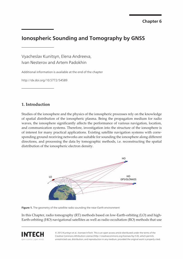
Figure 1. The geometry of the satellite radio sounding the near-Earth environment

In this Chapter, radio tomography (RT) methods based on low-Earth-orbiting (LO) and high-Earth-orbiting (HO) navigational satellites as well as radio occultation (RO) methods that use

© 2013 Kunitsyn et al.; licensee InTech. This is an open access article distributed under the terms of theCreative Commons Attribution License (http://creativecommons.org/licenses/by/3.0), which permitsunrestricted use, distribution, and reproduction in any medium, provided the original work is properly cited.

the data of quasi tangential sounding are considered. The “old” LO navigational systems(American Transit and Russian Tsikada) allow the receivers to determine their locationseverywhere on the Earth's surface, but not continuously. The time gap between the neighbor‐ing positioning determinations depends on the number of operational satellites in orbit. The“new” HO systems (GPS/GLONASS) are suitable for continuous worldwide positioningmeasurements. As far as spatial coverage is concerned, all satellite navigation systems areglobal. They are further referred to here as the Global Navigation Satellite Systems (GNSS).Note that at present, the term GNSS is mainly applied to HO navigation systems (the AmericanGPS and Russian GLONASS systems which are currently operational as well as EuropeanGalileo, Chinese BeiDou systems and Japanese QZSS.

Figure 1 depicts satellite radio probing of the near-Earth's environment that includes theatmosphere, the ionosphere, and the protonosphere. Transmitters onboard the LO and HOsatellites and the ground receivers provide the sets of rays intersecting the earth's near-spaceand allow determining the group and phase paths of the radio signals (in the case of LOsystems, only the phase paths) along the corresponding rays. The receivers onboard the LOsatellites that receive the radio transmissions from the HO satellites are also suitable fordetermining the group and phase paths of the signal along the set of the rays that are quasi-tangential to the Earth's surface. These measurements are suitable for sounding the near-spaceenvironment along various directions and calculating the integrals (or the differences of theintegrals) of the refraction index in the medium. This set of integrals can be inverted by the RTprocedure for the parameters of the medium. In the case of ionospheric sounding, the integralsof the refraction index are reduced to the integrals of the ionospheric electron density.

2. The methods of GNSS-based radio tomography

Methods of the satellite ionospheric radio tomography are being successfully developed atpresent [1-8]. Since the early 1990s, RT methods based on the LO navigation systems have beenoperational. In recent years, RT studies based on the measurements using HO navigationsystems have been extensively conducted [6-8]. Further in the text, various types of radiotomography are referred to as low-orbital RT and high-orbital RT (LORT and HORT).

2.1. Low orbital ionospheric radio tomography

Present-day navigational systems are based on the low orbiting satellites flying in near-circularorbits at an altitude of about 1000-1150 km. These utilize chains of ground-based receivers,which capture RT data along different rays. In RT experiments, the phase difference betweentwo coherent signals transmitted from the satellite at the frequencies of 150 and 400 MHz isrecorded at a set of receiving stations on the ground. The receivers are arranged in a chainparallel to the ground projection of the satellite track, the distance between the neighboringreceivers being typically a few hundred kilometers. The reduced phases ϕ recorded at thereceiving sites are the input data for the RT imaging. The integrals of the electron density N

Geodetic Sciences - Observations, Modeling and Applications224

along the rays linking the ground receivers with the onboard satellite transmitter are propor‐tional to the absolute (total) phase Φ [1, 2], which includes the unknown initial phase ϕ0:

0er Ndal s f f= F = +ò (1)

Here, λ is the wavelength of the satellite radio signal, dσ is the element of the ray, and re is theclassical electron radius. The scaling coefficient α (of the order of unity) depends on thesounding frequencies used. Equation (1) can be recast in the operator form [4] that includesthe typical uncorrelated measurement noise ξ:

PN x= F + (2)

where P is the projection operator mapping the two-dimensional (2D) distribution N to the setof one-dimensional (1D) projections Φ. Thus, the problem of tomographic inversion is reducedto the solution of the linear integral equations (2) for the electron concentration N . One of theprobable ways to solve (2) is to discretize (approximate) the projection operator P. This yieldsthe corresponding system of linear equations (SLE) with the discrete operator L:

LN =Φ + ξ + E , E =LN −PN (3)

where E is the approximation error that depends on the solution N itself. Note that equations(2) and (3) are equivalent if the approximation error E is known. However, in the case ofreconstructing the data of a real RT experiment, E is not known, and, in fact, quite a differentSLE is actually solved:

LN x= F + (4)

The system (4) is not equivalent to SLE (3). In other words, the difference between the solutionsof (3) and (4) ensues from the difference in both the quasi-noise component and the correlated(in time and rays) approximation error E . For SLE (4) to be solved, the absolute phase Φtogether with ϕ0 should be known. The errors in ϕ0 estimated by the different receivers canresult in the contradictory and inconsistent data, which leads to low-quality RT reconstruc‐tions. In order to avoid this difficulty, a method of phase-difference radio tomography (RTbased on the difference of the linear integrals along the neighboring rays) was developed [9],which does not require the initial phase ϕ0 to be determined. The SLE of the phase-differenceRT is determined by the corresponding difference:

' 'A L L DN N N x= - = F -F = + (5)

Ionospheric Sounding and Tomography by GNSShttp://dx.doi.org/10.5772/54589

225

where LN =Φ is the initial SLE and L'N =Φ ' is the system of linear equations along the set ofneighboring rays.

There are numerous algorithms, both direct and iterative, that solve SLEs (4) and (5). Atpresent, in the problems of ray radio tomography of the ionosphere, iterative algorithms aremost popular, although non-iterative algorithms are also used. These algorithms utilize asingular value decomposition with its modifications, regularization of the root mean square(RMS) deviation, orthogonal decomposition, maximum entropy, quadratic programming,Bayesian approach, etc. [3-7]. Extensive numerical modeling and LORT imaging of numerousexperimental data revealed the efficient combinations of various methods and the algorithmsthat yield the best reconstructions.

“Phase-difference” LORT provide much better results and higher sensitivity compared to“phase only” methods. This is confirmed by reconstructions of the experimental data as well[4, 7]. The horizontal and vertical resolution of LORT in its linear formulation is 20-30 km and30-40 km, respectively. If the refraction of the rays is taken into account, the spatial resolutionof LORT can be improved to 10-20 km [7].

2.2. High orbital ionospheric radio tomography

Deployment of the global navigational systems (GPS and GLONASS) in USA and Russia offersthe possibility to continuously measure trans-ionospheric radio signals and solve the inverseproblem of radio sounding [6-8]. In the near future, there are plans to launch the EuropeanGalileo and Chinese BeiDou satellite systems. Signals of the present-day GPS/GLONASS arecontinuously recorded at the regional and global receiving networks (e.g., the networkoperated by the International GNSS Service, IGS, which comprises about of two thousandreceivers). These data are suitable for reconstruction of the ionospheric electron density, thetotal electron content (TEC).

Inverse problems of radio sounding based on the GPS/GLONASS data, which pertain to thetomographic problems with incomplete data, are inherently high-dimensional. Due to therelatively low angular velocity of the high-orbiting satellites, allowance for the temporalvariations of the ionosphere becomes essential. This makes the RT problem four-dimensional(three spatial coordinates and time) and exacerbates incompleteness of the data: every pointin space is not necessarily traversed by the rays that link the satellites and the receivers,therefore the data gaps arise in the regions where only few receivers are available. The solutionof this problem requires special approaches [10].

The methods of ionospheric sounding typically analyze the phases of the radio signals thatpropagate from the satellite to the ground receiver at two coherent multiple frequencies. Forexample, in the GPS-based soundings, these frequencies are f1 = 1575.42 MHz and f2 = 1227.60MHz. The corresponding data (L1 and L2) are the phase paths of the radio signals measured inthe units of the wavelengths of the sounding signal. Another parameter that can be used inthe analysis is the pseudo-ranges (the group paths of the signals), which is the time taken bythe wave-trains at the frequencies f1 and f2 to propagate from the source to the receiver. The


phase delays L1 and L2 are proportional to the total electron content, TEC, the integral ofelectron density along the ray between the satellite and the receiver:

2 21 2 1 2

2 21 2 1 2

,L L f f cTEC constf f Kf f

æ ö= - +ç ÷ç ÷ -è ø

(6)

where K = 40.308 m3s-2 and c = 3‧108 m/s is the speed of light in vacuum. Note that, by usingthe phase delay data, it is only possible to calculate the TEC value up to a certain constantindicated as the additive term in formula (6). The relationship (6) is similar to formula (1) withthe unknown constant in the right-hand side of the system.

TEC values can also be derived from the pseudo-ranges P1 and P2 [11]:

2 1

2 22 1

1 1

P PTEC

Kf f

-=

æ ö-ç ÷ç ÷

è ø

(7)

However, compared to phase data, the pseudo-range data are strongly distorted and conta‐minated by noise. The noise level in P1 and P2 is typically 20-30% and even higher, while in thephase data it is below 1% and rarely reaches a few percent. Therefore, for HORT, the phasedata are preferable.

Most authors [6] solve the HORT problem using a set of linear integrals. In that approach, itis assumed that the TEC data are sufficiently accurately determined from the phase and groupdelay data (6, 7). However, the absolute TEC (7) is determined with a large uncertainty incontrast to the TEC differences that are calculated highly accurately. Therefore, the phase-difference approach was applied in this case, too [10, 12]. In other words, instead of the absoluteTEC, its corresponding differences or the time derivatives dTEC/dt were used as input datafor the RT problem.

The problem of the 4-D GNSS-based radio tomography can be solved by the approachdeveloped in 2-D LORT. In this approach, the electron density distribution is represented interms of a series expansion of the certain local basis functions; in this case, the set of the linearintegrals or their differences is transformed into SLE. However, in contrast to 2-D LORT, hereit is necessary to introduce an additional procedure interpolating the solutions in the area withmissing data. The implementation of this approach in the regions covered by dense receivingnetworks (e.g., North America and Europe) with a rather coarse calculation grid and suitablesplines of varying smoothness [10,12] has proved highly efficient.

Another approach seeks sufficiently smooth solutions of the problem so that the algorithmsprovide a good interpolation in the area with missing data. For example, let us consider aSobolev norm and seek a solution that minimizes this norm over the infinite set of solutionsof the initial (underdetermined) tomographic problem (5):


227

20A D, minnWAN D

N f f=

= - (8)

Here, function f is the solution with a given weight .

Practical implementation of this approach faces difficulties associated with solution of theconstrained minimization problem. The direct approach utilizing the method of Lagrange'sundetermined multipliers gives SLE with high-dimensional (due to the great number of rays)matrices, which do not possess any special structure that would simplify the solution.Therefore, we solve this minimization problem by an iterative method [10] that is a version ofthe SIRT technique, with additional smoothing (by filtering) of iterative increments over thespatial variables. This method allows for use of a-priori information that can be introducedboth through the initial approximation for the iterations and through weighting coefficientsthat determine the relative intensity of electron density variations at different heights.

Computer-aided modeling shows that quasi-stationary ionospheric structures can be recon‐structed with reasonable accuracy, although HORT has a significantly lower resolution thanLORT. As a rule, the vertical and horizontal resolution of HORT is 100 km at best, and the timestep (the interval between two consecutive reconstructions) is typically 20 - 60 minutes. Inregions covered by dense receiving networks (Europe, USA, and Alaska), the resolution canbe improved to 30-50 km with a 10 - 30 minute interval between consecutive reconstructions.Resolution of 10-30 km with a time step of 2 minutes can only be achieved in the regions withvery dense receiving networks (California and Japan).

3. Testing and validation of ionospheric radio tomography

In numerous experiments, RT images of the ionosphere have been compared with corre‐sponding parameters (vertical profiles of electron density and critical frequences) measuredby ionosondes [13-18, 4, 19, 7]. In most cases, the RT results closely agree with ionosonde datawithin the limitations of the accuracy of both methods. An example of such a comparison withthe world's first RT reconstruction of an ionospheric trough is presented in Figure 2. Here, thedots show the vertical profile of electron density according to measurements by an ionosondein Moscow, and the solid line displays the corresponding profile calculated from the RTreconstruction for April 7, 1990 (22:05 LT).

A comparison of a few hundred ionospheric RT cross-sections in the region of the equatorialanomaly with observations by two ionosondes in October-November 1994 [19] is illustratedin Figure 3. The distributions of electron density were reconstructed from RT measurementsat the low-latitude Manila-Shanghai chain, which included six receivers arranged along themeridian 121.1±1ºE within the latitude band between 14.6ºN and 31.3ºN. One ionosonde wasinstalled at 25.0ºN, 121.2ºE 7.5 km of Chungli almost in the middle of the chain. Anotherionospheric station was located in the southernmost part of the chain in Manila (14.7ºN,121.1ºE).


Figure 2. Vertical profiles of electron density in Moscow at 22:05 LT on April 7, 1990, depicting both radio tomogra‐phy and ionosonde data.

Using RT reconstructions, maximal electron densities and plasma frequencies f0F2 werecalculated in the vicinities of the ionospheric stations. These parameters were then comparedto the corresponding values determined from ionosonde measurements. These two data setsare compared in Figure 3. The points that lie on the bisectix of the right angle correspond tothe case where the RT-based and the ionosonde-based critical frequencies exactly coincide. Wealso calculated the normalized root mean square (rms) deviations of the RT-based criticalfrequencies f0F2 from the corresponding values inferred from the ionosonde measurements.

Figure 3. The comparison between the plasma frequencies f0F2 calculated from the RT reconstructions and the corre‐sponding values derived from the measurements by the ionosondes in (left) Chungli and (right) Manila for October-November 1994.

A detailed analysis reveals the following points.


229

1. The scatter in f0F2 in Chungli is larger than in Manila. The normalized rms deviations forthe ionosondes in Chungli and Manila are 11.2% and 8.9%, respectively.

2. In the case of high electron concentrations, especially for f0F2 above 13 MHz, the experi‐mental points tend to saturation: the critical frequencies f0F2 derived from RT fall short ofthe corresponding values calculated from the ionosonde measurements.

These features indicate that strong spatial gradients in electron density typical in the region ofthe equatorial anomaly can cause the discrepances in the plasma frequencies calculated fromRT and ionosonde measurements.

In experiments on vertical pulsed sounding of the ionosphere, the signal is not reflected fromdirectly overhead. Even in the case of vertical sounding of a horizontally stratified ionosphere,the ordinary wave tends to deviate toward the pole, and in the point of reflection, it becomesperpendicular to the local geomagnetic field [20]. Therefore, in the general case, reflection doesnot occur vertically above the sounding point but somewhat away from overhead.

Zero offsets are only observed at the equator, while in the region of the Chungli ionosonde,the offset can be ~10 km. In addition, Chungli is located close to the maximum of the equatorialanomaly, which is marked by very strong gradients. Therefore, the sounding ray of the Chungliionosonde will significantly deflect before having been reflected backwards. Therefore, thevalues of f0F2 recorded by the Chungli ionosonde will by no means be the actual f0F2 valuesexactly overhead. These considerations will help us to interpret the results of comparison ofplasma frequencies.

First, at high plasma frequencies (f0F2 higher than 13 MHz), the experimental points in Figure3 fall below the bisectrix. This area relates to the stage of a completely mature anomaly with awell-developed crest and, therefore, with strong gradients in electron density. It is due to thesegradients that the values of f0F2 determined from the ionosondes are, on average, overesti‐mated compared to the actual critical frequencies f0F2 overhead.

Second, values of f0F2 at Chungli demonstrate a larger scatter than at Manila. Since Chungli islocated in the central part of the RT chain, the most reliable RT reconstructions are expectedat the latitudes near the middle segment of the chain (close to Chungli) rather than on itsmargins (Manila). This contradicts the actual results shown in Figure 3. On the other hand,Chungli is located in the vicinity of the peak electron density within the crest of the anomaly,in the area of strong gradients, where errors of vertical sounding (associated with deflectionof the reflected ray) are most probable. Therefore, large discrepances in the Chungli region arequite probable, which is confirmed by Figure 3.

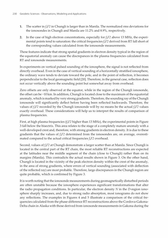
It is worth noting that the ionosonde measurements during geomagnetically disturbed periodsare often unstable because the ionosphere experiences significant transformations that alterthe radio propagation conditions. In particular, the electron density N in the D-region iono‐sphere sharply increases, and, due to strong radio absorption, most ionograms do not showany reflections. The examples in Figures 4 and 5 illustrate a comparison of the critical fre‐quencies calculated from the phase-difference RT reconstructions above the Cordova-Gakona-Delta chain in Alaska with those derived from ionosonde measurements in Gakona during the


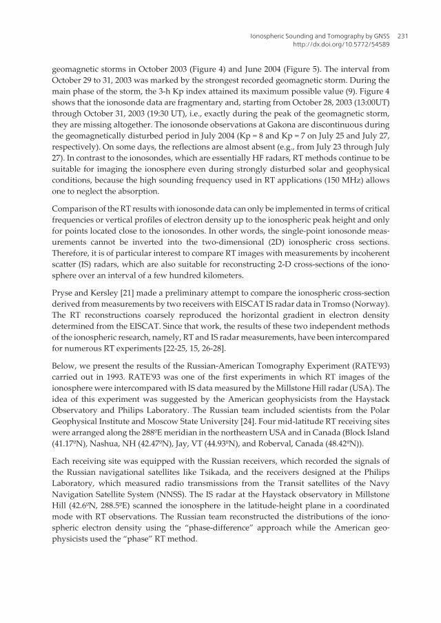
geomagnetic storms in October 2003 (Figure 4) and June 2004 (Figure 5). The interval fromOctober 29 to 31, 2003 was marked by the strongest recorded geomagnetic storm. During themain phase of the storm, the 3-h Kp index attained its maximum possible value (9). Figure 4shows that the ionosonde data are fragmentary and, starting from October 28, 2003 (13:00UT)through October 31, 2003 (19:30 UT), i.e., exactly during the peak of the geomagnetic storm,they are missing altogether. The ionosonde observations at Gakona are discontinuous duringthe geomagnetically disturbed period in July 2004 (Kp = 8 and Kp = 7 on July 25 and July 27,respectively). On some days, the reflections are almost absent (e.g., from July 23 through July27). In contrast to the ionosondes, which are essentially HF radars, RT methods continue to besuitable for imaging the ionosphere even during strongly disturbed solar and geophysicalconditions, because the high sounding frequency used in RT applications (150 MHz) allowsone to neglect the absorption.

Comparison of the RT results with ionosonde data can only be implemented in terms of criticalfrequencies or vertical profiles of electron density up to the ionospheric peak height and onlyfor points located close to the ionosondes. In other words, the single-point ionosonde meas‐urements cannot be inverted into the two-dimensional (2D) ionospheric cross sections.Therefore, it is of particular interest to compare RT images with measurements by incoherentscatter (IS) radars, which are also suitable for reconstructing 2-D cross-sections of the iono‐sphere over an interval of a few hundred kilometers.

Pryse and Kersley [21] made a preliminary attempt to compare the ionospheric cross-sectionderived from measurements by two receivers with EISCAT IS radar data in Tromso (Norway).The RT reconstructions coarsely reproduced the horizontal gradient in electron densitydetermined from the EISCAT. Since that work, the results of these two independent methodsof the ionospheric research, namely, RT and IS radar measurements, have been intercomparedfor numerous RT experiments [22-25, 15, 26-28].

Below, we present the results of the Russian-American Tomography Experiment (RATE'93)carried out in 1993. RATE'93 was one of the first experiments in which RT images of theionosphere were intercompared with IS data measured by the Millstone Hill radar (USA). Theidea of this experiment was suggested by the American geophysicists from the HaystackObservatory and Philips Laboratory. The Russian team included scientists from the PolarGeophysical Institute and Moscow State University [24]. Four mid-latitude RT receiving siteswere arranged along the 288ºE meridian in the northeastern USA and in Canada (Block Island(41.17ºN), Nashua, NH (42.47ºN), Jay, VT (44.93ºN), and Roberval, Canada (48.42ºN)).

Each receiving site was equipped with the Russian receivers, which recorded the signals ofthe Russian navigational satellites like Tsikada, and the receivers designed at the PhilipsLaboratory, which measured radio transmissions from the Transit satellites of the NavyNavigation Satellite System (NNSS). The IS radar at the Haystack observatory in MillstoneHill (42.6ºN, 288.5ºE) scanned the ionosphere in the latitude-height plane in a coordinatedmode with RT observations. The Russian team reconstructed the distributions of the iono‐spheric electron density using the “phase-difference” approach while the American geo‐physicists used the “phase” RT method.


231

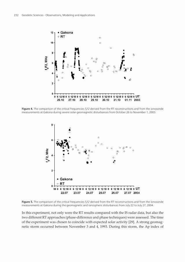
Figure 4. The comparison of the critical frequencies f0F2 derived from the RT reconstructions and from the ionosondemeasurements at Gakona during severe solar-geomagnetic disturbances from October 26 to November 1, 2003.

Figure 5. The comparison of the critical frequencies f0F2 derived from the RT reconstructions and from the ionosondemeasurements at Gakona during the geomagnetic and ionospheric disturbances from July 22 to July 27, 2004.

In this experiment, not only were the RT results compared with the IS radar data, but also thetwo different RT approaches (phase-difference and phase techniques) were assessed. The timeof the experiment was chosen to coincide with expected solar activity [29]. A strong geomag‐netic storm occurred between November 3 and 4, 1993. During this storm, the Ap index of


planetary geomagnetic activity reached 111 nT, and during the main phase of the storm, the3-h Kp index was 6.7.

The results of RATE'93 demonstrated the high quality of the RT ionospheric cross-sectionsreconstructed by the phase difference method [24]. It should be noted that RT cross-sectionsand radar ionospheric images are clearly similar in the case of a smooth, almost regularionosphere with insignificant local extrema. Further in the text, the results are visualized inthe coordinates “height h above the Earth's surface (in km) - latitude.” Figure 6 presents thecross-sections of the ionosphere about 1 hour 45 minutes after the sudden storm commence‐ment (at 23:00 UT on November 3, 1993). The ionospheric cross-section based on the IS radardata is displayed in Figure 6 (upper panel), and the phase-difference RT reconstruction isshown in Figure 6 (lower panel).

A characteristic trough appeared about 44ºN, and the ionozation sharply increased in theheight interval from 200 km to 300 km near 47ºN, due to precipitation of low-energy particlesbetween 46ºN and 51ºN [29]. Figure 6 shows that the RT cross-section closely agrees with theradar ionospheric image. However, it should be noted that radar measurements are limited tothe height interval from 180 km (below which the concentrations are insignificant) to 600 km(above which the distortions and noise level are very high) [29].

The similarity of the RT cross-sections and radar ionospheric images (Figure 6) confirms thatthe increase in the radar signal in the bottom F-region ionosphere reflects the actual enhance‐ment of electron density substantially below 300 km, but not the noise or coherent backscatterfrom the irregularities associated with the E-region electric fields [24, 29]. Moreover, bothionospheric cross-sections in Figure 6 clearly demonstrate the elevated F-region south of 45ºN.The elevation increases with increasing distance to the trough. The elevation in the RTreconstruction attains 400-450 km and is larger than in the radar image.

Figure 6 (upper panel) shows the preliminary radar-based ionospheric cross-section aspublished in [24]. The difference between the reconstructions is 32.6%, which falls within theaccuracy of both methods. However, it should be noted that the ionospheric cross-sectionsbased on radar data and those reconstructed from the RT measurements do not correspond tothe same time interval but are somewhat spaced in time. The time shift between them is 5minutes, which is quite a significant value considering that the measurements were conductedduring the period of active structural rearrangement of the ionosphere on November 4, 1993.

In their later paper, Foster and Rich [29] quote the final radar cross section that was recon‐structed after scrupulous analysis of the measurements. On that image, the bottom of theionospheric F-layer is obseved at the same height as in the RT image shown in Figure 6 (lowerpanel), i.e., at 400-450 km. According to the radar data, the F-layer remained elevated for ashort lapse of time (~20 minutes).

In this experiment, a narrow (<2º) tilted trough was detected by both RT and radar observa‐tions at a latitude of 41º-42º at 04:56UT on November 4, 1993. Phase-difference tomographyalso revealed a border about 50 km in size on the northern wall of the trough, which has notbeen distinguished by the radar observations [24]. This means that the phase-difference RTmethod has higher horizontal resolution. The border clearly manifests itself in the phase of


233

the signal recorded at the Nashua receiving site (Figure 7), where it produces a local maxi‐mum at about 41.5º-42ºN. In contrast to the phase-difference RT, all the ionospheric imagesreconstructed by the phase RT are similar to each other and close to the PIM model [30]. Dueto errors in the determination of the initial phases, the phase RT method does not even re‐veal the troughs themselves. The comparison shows that the cross-sections of electron densi‐ty reconstructed by the phase-difference RT and the ionospheric images derived from the ISradar data agree within the accuracy of both methods. Moreover, compared to the IS meth‐od, phase-difference RT has a higher horizontal resolution. However, the IS radar revealedthin (<50 km) extended horizontal layers which are not resolved by radio tomography dueto the insufficient base of the RT measurements (the distance between the outermost receiv‐ers in the experiment was only 800 km) and a quasi-tangential (to the Earth's surface) rayswere absent.

Figure 6. Cross sections of the ionosphere after sudden commencement of the geomagnetic storm (00:45 UT on No‐vember 4, 1993): (a) according to the radar data; (b) according to phase-difference RT.

This experiment also demonstrated that the method of phase-difference RT has noticeableadvantages (in sensitivity and quality of the reconstructions) over the phase radio tomogra‐phy which uses linear integrals. A comprehensive intercomparison between the results ofphase tomography, phase-difference tomography, and IS radar studies is presented in thefinal summarizing paper [24].


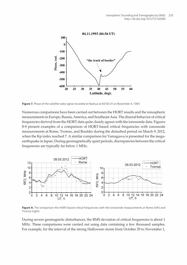
Figure 7. Phase of the satellite radio signal recorded at Nashua at 04:56 UT on November 4, 1993

Numerous comparisons have been carried out between the HORT results and the ionosphericmeasurements in Europe, Russia, America, and Southeast Asia. The diurnal behavior of criticalfrequencies derived from the HORT data quite closely agrees with the ionosonde data. Figures8-9 present examples of a comparison of HORT-based critical frequencies with ionosondemeasurements at Rome, Tromso, and Boulder during the disturbed period on March 9, 2012,when the Kp index reached 7. A similar comparison for Yamagawa is presented for the mega-earthquake in Japan. During geomagnetically quiet periods, discrepancies between the criticalfrequencies are typically far below 1 MHz.

Figure 8. The comparison the HORT-based critical frequencies with the ionosonde measurements at Rome (left) andTromso (right)

During severe geomagnetic disturbances, the RMS deviation of critical frequencies is about 1MHz. These comparisons were carried out using data containing a few thousand samples.For example, for the interval of the strong Halloween storm from October 29 to November 1,


235

2003, with measurements from 13 North American ionosondes, the RMS deviation of thecritical frequencies was 1.7 MHz [31].

Figure 9. Comparison of HORT-based critical frequencies with ionosonde measurements at Boulder (left) and Yama‐gawa (right)

4. Examples of the GNSS-based ionospheric radio tomography

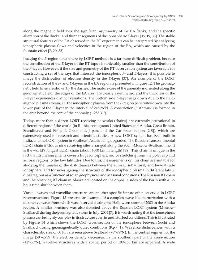
The world's first LORT images were reconstructed in March-April 1990 by geophysicists ofthe Moscow State University and Polar Geophysical Institute of the Russian Academy ofSciences [32]. One of the first RT cross sections of the ionosphere between Moscow andMurmansk is presented in Figure 10. The horizontal axis in this plot shows the latitudes, andthe vertical axis, the heights. The ionospheric electron density is given in units of 1012 m3. Thisimage clearly shows a proto-typical ionospheric trough at about 63º--65ºN and a local extrem‐um within it. Further experiments revealed the complex and diverse structure and dynamicsof the ionospheric trough [1-8]. In 1992, preliminary results in RT imaging of the ionospherewere obtained by colleagues from the UK [21]. The LORT-based studies and applications drewsignificant interest from geophysicists around the globe. At the present time, more than tenresearch teams in different countries are engaged in these investigations [3-7]. Series of LORTexperiments carried out in Europe, America, and Southeast Asia during the last twenty years[3-8] have demonstrated the high efficiency of radio tomographic methods for study of diverseionospheric structures.

Quite often, RT images of the ionosphere in different regions reveal the well-known wavestructures - traveling ionospheric disturbances (TID). The example in Figure 11 depicts an RTionospheric image with distinct TIDs having a typical slope of 45º, as recorded on the Moscow-Arkhangelsk RT link [33]. Here, the ionosphere is quite moderately modulated by the TIDs(the modulation depth is 25-30%). Such TIDs are often observed in RT reconstructions, asmentioned in [5, 34].

RT experiments in Southeast Asia at the low-latitude Manila-Shanghai chain revealed a seriesof characteristic features in the structure of the equatorial anomaly (EA) including the post-noon alignment of the mature core of the EA (the area close to the peak electron concentration)


along the magnetic field axis; the significant asymmetry of the EA flanks, and the specificalteration of the thicker and thinner segments of the ionospheric F-layer [35, 19, 36]. The stablestructural features of the EA observed in the RT experiments can be interpreted by analyzingionospheric plasma flows and velocities in the region of the EA, which are caused by thefountain effect [7, 20, 35].

Imaging the E-region ionosphere by LORT methods is a far more difficult problem, becausethe contribution of the E-layer in the RT input is noticeably smaller than the contribution ofthe F-layer. However, if the size and geometry of the RT observation system are favorable forconstructing a set of the rays that intersect the ionospheric F- and E-layers, it is possible toimage the distribution of electron density in the E-layer [37]. An example of the LORTreconstruction of the F- and E-layers in the EA region is presented in Figure 12. The geomag‐netic field lines are shown by the dashes. The mature core of the anomaly is oriented along thegeomagnetic field; the edges of the EA crest are clearly asymmetric, and the thickness of theF-layer experiences distinct variations. The bottom side F-layer sags down due to the field-aligned plasma stream, i.e. the ionospheric plasma from the F-region penetrates down into thelower part of the E-layer in the interval of 24º-26ºN. A constriction (“isthmus”) is formed inthe area beyond the core of the anomaly (~ 28º-31º).

Today, more than a dozen LORT receiving networks (chains) are currently operational indifferent regions of the world (in Russia, contiguous United States and Alaska, Great Britain,Scandinavia and Finland, Greenland, Japan, and the Caribbean region [2-8]), which areextensively used for research and scientific studies. A new LORT system has been built inIndia, and the LORT system in Southeast Asia is being upgraded. The Russian transcontinentalLORT chain includes nine receiving sites arranged along the Sochi-Moscow-Svalbard line. Itis the world's longest LORT chain (about 4000 km in length) [38]. This chain is unique in thefact that its measurements cover a huge ionospheric sector stretching from the polar cap andauroral regions to the low latitudes. Due to this, measurements on this chain are suitable forstudying the transfer of the disturbances between the auroral, subauroral, and low-latitudeionosphere, and for investigating the structure of the ionospheric plasma in different latitu‐dinal regions as a function of solar, geophysical, and seasonal conditions. The Russian RT chainand the receiving RT chain in Alaska are located on the opposite sides of the Earth with a 12-hour time shift between them.

Various waves and wavelike structures are another specific feature often observed in LORTreconstructions. Figure 13 presents an example of a complex wave-like perturbation with adistinctive wave-front which was observed during the Halloween storm of 2003 in the Alaskaregion. A similar structure was also detected above the Russian LORT system (Moscow-Svalbard) during the geomagnetic storm in July, 2004 [7]. It is worth noting that the ionosphericplasma can be highly complex in its structure even in undisturbed conditions. This is illustratedby Figure 14 which shows the LORT cross section of the ionosphere between Sochi andSvalbard during geomagnetically quiet conditions (Kp < 1). Wavelike disturbances with acharacteristic size of 50 km are seen above Svalbard (78º-79ºN). In the central segment of theimage (59º-65ºN) the electron density decreases. In the southern part of the cross-section(42º-55ºN), wavelike structures with a spatial period of 100-150 km are apparent. A wide


237

ionization trough in the interval of 62º-64ºN is observed on the LORT reconstruction in Figure15. The local maximum at 65º-66ºN is almost merged with the polar wall of the trough. A spotof enhanced ionization is identified within the trough about 63º-64ºN latitude. And, wavelikedisturbances are revealed throughout 66º-78ºN.

Besides being suitable for reconstructing the large-scale ionospheric phenomena of natu‐ral origin, LORT is also efficient for tracking artificial ionospheric disturbances. TheLORT cross-section in Figure 16 shows wavelike structures that formed in the ionospherewithin 30 minutes after launch of a rocket from the Plesetsk Cosmodrome. The cosmo‐drome is located approximately 63ºN (200 km) distant from the satellite ground track.These anthropomorphic disturbances have a very complex structure wherein large irregu‐larities (200-400 km) coexist with smaller ionospheric features (50-70 km), and the slopeof the “wavefront” is also varying. Wave disturbances generated by launching high-pow‐er rocket vehicles are described in [39] where it is shown that ignition of the rocket gen‐erates acoustic-gravity waves (AGW) which, in turn, induce corresponding perturbationsin electron density. During RT experiments wtih the Moscow-Murmansk chain, long-lived local disturbances in the ionospheric plasma were also identified above sites whereground industrial explosions were carried out [40].

RT methods revealed generation of ionospheric disturbances by the Sura ionosphericheating facility, which radiated high-power HF waves, modulated with a 10-minuteheat/off cycles [41]. Figure 17 shows an ionospheric cross-section through a typical heat‐ed area. A narrow trough in the ionization, aligned with the propagation direction of theheating HF wave, is identified. Traveling ionospheric disturbances associated with theacoustic gravity waves (AGWs) generated by the Sura heater are observed divergingfrom the heated area. Unfortunately, insufficient density of HO receivers in central Rus‐sia prevented us from obtaining high-quality HORT images of the ionosphere during thisheating experiment; however, the data recorded by the few available receivers supportpresence of the AGWs [41].

Thus, LORT is capable of reconstructing nearly instantaneous 2-D snapshots of the electrondensity distribution in the ionosphere (which actually cover a time span of 5-15 minutes). Thetime interval between the successive RT reconstructions depends on the number of theoperational satellites and, as of now is 30-120 minutes. The LORT method is also suitable fordetermining plasma flows by analyzing successive RT cross sections of the ionosphere [42].An optimal LORT receiving system, consisting of several parallel chains located within a fewhundred km of each other, would allow 3-D imaging of the ionosphere. The requirement formultiple receiving chains is the major limitation of LORT.

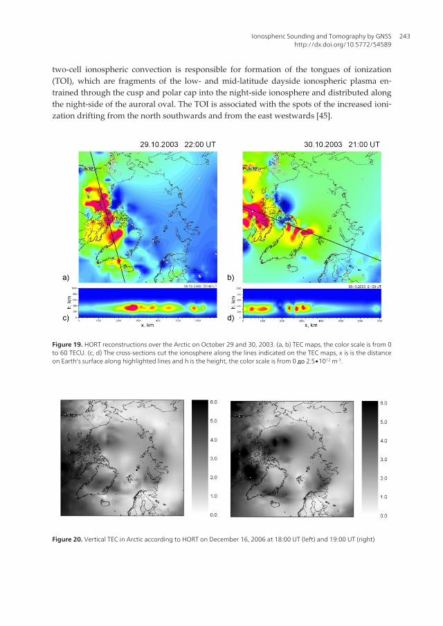
The reconstructions presented below illustrate the possibilities of newly developedHORT techniques. Figure 18 displays the evolution of the ionospheric trough above Eu‐rope in the evening on April 17, 2003. The TEC maps and the meridional cross sectionsalong 21ºE show the trough widening against the background, with an overall nighttimedecrease in electron density.


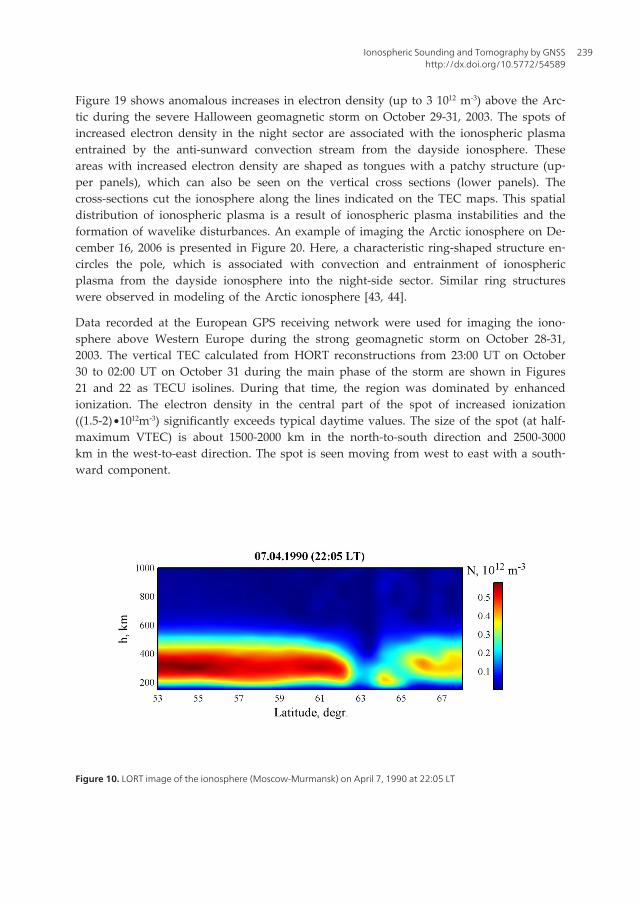
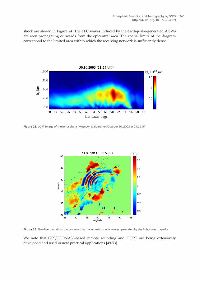
Figure 19 shows anomalous increases in electron density (up to 3 1012 m-3) above the Arc‐tic during the severe Halloween geomagnetic storm on October 29-31, 2003. The spots ofincreased electron density in the night sector are associated with the ionospheric plasmaentrained by the anti-sunward convection stream from the dayside ionosphere. Theseareas with increased electron density are shaped as tongues with a patchy structure (up‐per panels), which can also be seen on the vertical cross sections (lower panels). Thecross-sections cut the ionosphere along the lines indicated on the TEC maps. This spatialdistribution of ionospheric plasma is a result of ionospheric plasma instabilities and theformation of wavelike disturbances. An example of imaging the Arctic ionosphere on De‐cember 16, 2006 is presented in Figure 20. Here, a characteristic ring-shaped structure en‐circles the pole, which is associated with convection and entrainment of ionosphericplasma from the dayside ionosphere into the night-side sector. Similar ring structureswere observed in modeling of the Arctic ionosphere [43, 44].

Data recorded at the European GPS receiving network were used for imaging the iono‐sphere above Western Europe during the strong geomagnetic storm on October 28-31,2003. The vertical TEC calculated from HORT reconstructions from 23:00 UT on October30 to 02:00 UT on October 31 during the main phase of the storm are shown in Figures21 and 22 as TECU isolines. During that time, the region was dominated by enhancedionization. The electron density in the central part of the spot of increased ionization((1.5-2)∙1012m-3) significantly exceeds typical daytime values. The size of the spot (at half-maximum VTEC) is about 1500-2000 km in the north-to-south direction and 2500-3000km in the west-to-east direction. The spot is seen moving from west to east with a south‐ward component.

Figure 10. LORT image of the ionosphere (Moscow-Murmansk) on April 7, 1990 at 22:05 LT


239

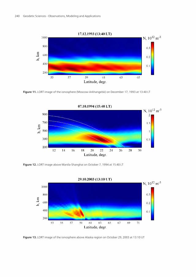
Figure 11. LORT image of the ionosphere (Moscow-Arkhangelsk) on December 17, 1993 at 13:40 LT

Figure 12. LORT image above Manila-Shanghai on October 7, 1994 at 15:40 LT

Figure 13. LORT image of the ionosphere above Alaska region on October 29, 2003 at 13:10 UT


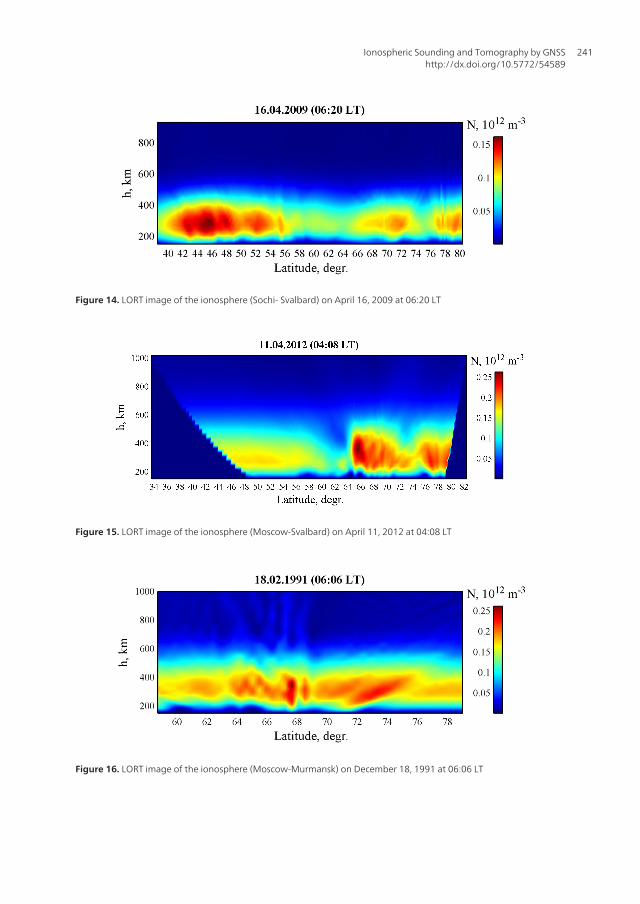
Figure 14. LORT image of the ionosphere (Sochi- Svalbard) on April 16, 2009 at 06:20 LT

Figure 15. LORT image of the ionosphere (Moscow-Svalbard) on April 11, 2012 at 04:08 LT

Figure 16. LORT image of the ionosphere (Moscow-Murmansk) on December 18, 1991 at 06:06 LT


241

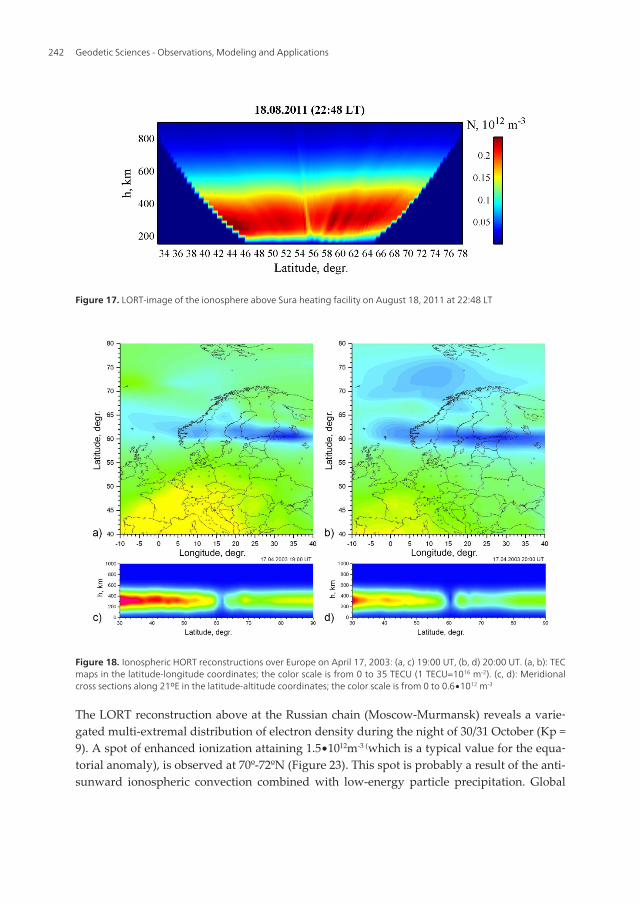
Figure 17. LORT-image of the ionosphere above Sura heating facility on August 18, 2011 at 22:48 LT

Figure 18. Ionospheric HORT reconstructions over Europe on April 17, 2003: (a, c) 19:00 UT, (b, d) 20:00 UT. (a, b): TECmaps in the latitude-longitude coordinates; the color scale is from 0 to 35 TECU (1 TECU=1016 m-2). (c, d): Meridionalcross sections along 21ºE in the latitude-altitude coordinates; the color scale is from 0 to 0.6∙1012 m-3

The LORT reconstruction above at the Russian chain (Moscow-Murmansk) reveals a varie‐gated multi-extremal distribution of electron density during the night of 30/31 October (Kp =9). A spot of enhanced ionization attaining 1.5∙1012m-3 (which is a typical value for the equa‐torial anomaly), is observed at 70º-72ºN (Figure 23). This spot is probably a result of the anti-sunward ionospheric convection combined with low-energy particle precipitation. Global


two-cell ionospheric convection is responsible for formation of the tongues of ionization(TOI), which are fragments of the low- and mid-latitude dayside ionospheric plasma en‐trained through the cusp and polar cap into the night-side ionosphere and distributed alongthe night-side of the auroral oval. The TOI is associated with the spots of the increased ioni‐zation drifting from the north southwards and from the east westwards [45].

Figure 19. HORT reconstructions over the Arctic on October 29 and 30, 2003. (a, b) TEC maps, the color scale is from 0to 60 TECU. (c, d) The cross-sections cut the ionosphere along the lines indicated on the TEC maps, x is is the distanceon Earth's surface along highlighted lines and h is the height, the color scale is from 0 до 2.5∙1012 m-3.

Figure 20. Vertical TEC in Arctic according to HORT on December 16, 2006 at 18:00 UT (left) and 19:00 UT (right)


243

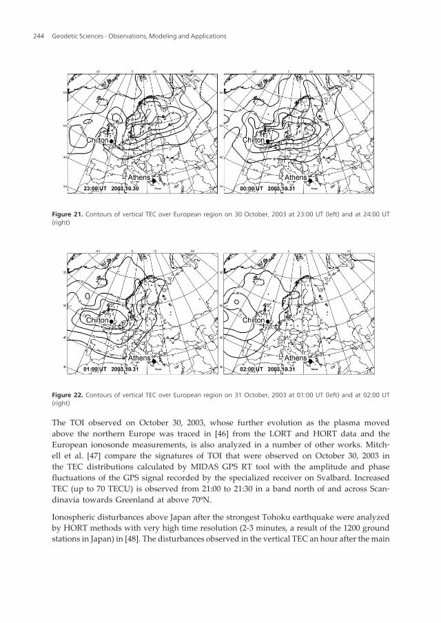
Figure 21. Contours of vertical TEC over European region on 30 October, 2003 at 23:00 UT (left) and at 24:00 UT(right)

Figure 22. Contours of vertical TEC over European region on 31 October, 2003 at 01:00 UT (left) and at 02:00 UT(right)

The TOI observed on October 30, 2003, whose further evolution as the plasma movedabove the northern Europe was traced in [46] from the LORT and HORT data and theEuropean ionosonde measurements, is also analyzed in a number of other works. Mitch‐ell et al. [47] compare the signatures of TOI that were observed on October 30, 2003 inthe TEC distributions calculated by MIDAS GPS RT tool with the amplitude and phasefluctuations of the GPS signal recorded by the specialized receiver on Svalbard. IncreasedTEC (up to 70 TECU) is observed from 21:00 to 21:30 in a band north of and across Scan‐dinavia towards Greenland at above 70ºN.

Ionospheric disturbances above Japan after the strongest Tohoku earthquake were analyzedby HORT methods with very high time resolution (2-3 minutes, a result of the 1200 groundstations in Japan) in [48]. The disturbances observed in the vertical TEC an hour after the main


shock are shown in Figure 24. The TEC waves induced by the earthquake-generated AGWsare seen propagating outwards from the epicentral area. The spatial limits of the diagramcorrespond to the limited area within which the receiving network is sufficiently dense.

Figure 23. LORT image of the ionosphere (Moscow-Svalbard) on October 30, 2003 at 21:25 UT

Figure 24. The diverging disturbance caused by the acoustic gravity waves generated by the Tohoku earthquake

We note that GPS/GLONASS-based remote sounding and HORT are being extensivelydeveloped and used in new practical applications [49-53].


245

5. Combination with other sounding techniques

Existing systems (FormoSat-3/COSMIC and a few others are capable of recording GNSS signalsonboard low-Earth orbiting satellite platforms). These satellites effectively demonstrate theradio occultation technique (OT) which acquires quasi-tangential projections of electrondensity N [54-56]. The OT method, coupled with subsequent ground reception of the OT data,opens up the possibility of sounding the ionosphere in a wide range of different geometries ofthe transmitting and receiving systems. The OT method provides integrals of N over a set ofquasi-tangential rays (the satellite-satellite links), and is a particular case of the RT method. Itis, however, necessary to construct a procedure for synthesizing the occultation data into thegeneral RT process [7, 8, 57]. The combination of RT and OT, when the RT data are supple‐mented by the satellite-to-satellite sounding (OT) data, would noticeably improve the verticalresolution of the RT reconstructions.

Existing ultra-violet (UV)-sounding systems (GUVI, SSULI, FormoSat-3/COSMIC) provideintegrals of N squared. UV sounding data can be incorporated into the general tomographiciterative scheme. For example, at the first step of a reconstruction, the main iteration isaccomplished with linear integrals and RT data alone. Then, based on the distribution ofelectron density N obtained in the first iteration, we run the iterative scheme for N squaredwith the UV input. Third, we transform the distribution of N squared derived at this step ofthe reconstruction into the distribution of N (the result of the second iteration); since thisdistribution can be used further. Thus, the odd iterations will work with the radio soundingdata, while even iterations will use UV input. Overall, we obtain a tomographic methodologywhich uses both radio sounding and UV sounding data. However, in order to ensure conver‐gence and to obtain high-quality final results, the experimental data of different kinds shouldbe consistent and have commensurate accuracy, otherwise the additional iterations based onthe “bad” data will degrade the result. Unfortunately, as of now, the UV data are far lessaccurate that the navigation radio sounding data.

Note that the RT methods described here refer to “ray” tomography [1] that neglects diffractioneffects. In previous work, we developed methods for diffraction tomography and statisticaltomography [1, 2, 4, 7]. Diffraction tomography is applicable for imaging the structure ofisolated localized irregularities with allowance for diffraction effects. Statistical tomographyreconstructs the spatial distributions of the statistical parameters of the randomly irregularionosphere [7, 58].

6. Conclusions

This Chapter briefly outlines the results of tomographic studies of the ionosphere conductedwith the participation of the authors. The methods applied in satellite radio tomography ofthe near-Earth plasma, including LORT and HORT, are described. During the last two decades,numerous RT experiments, studying the equatorial, mid-latitude, sub-auroral, and auroralionosphere were carried out in different regions of the world (in Europe, USA, and Southeast


Asia). Examples of RT images of the ionospheric electron density based on data recorded in aseries of RT experiments have been presented.

An RT system is a distributed sounding system: the moving satellites with onboard transmit‐ters and receivers together with the ground receiving networks enable continuous soundingof the medium along different directions and support imaging of the spatial structure of theionosphere. Satellite RT, utilizing a system of ground and satellite receivers, combined withtraditional means of ionospheric sounding provides the basis for regional and global moni‐toring of the near-Earth plasma.

Acknowledgements

We are grateful to professors L.-C. Tsai and C.H. Liu, our colleagues from the Center for Spaceand Remote Sensing Research (National Central University, Chungli, Taiwan), and theUniversity of Illinois at Urbana Champaign for providing experimental data. We acknowledgeuse of the worldwide ionosonde database accessed from the National Geophysical Data Center(NGDC) and Space Physics Interactive Data Resource (SPIDR). The authors are grateful toNorth-West Research Associates (NWRA) for providing experimental relative TEC data in theAlaska region. This work was supported by the Russian Foundation for Basic Research (grants13-05-01122, 11-05-01157), the Ministry for Education and Science of the Russian Federation(project 14.740.11.0203), a grant of the President of Russian Federation (projectМК-2544.2012.5), and M.V. Lomonosov Moscow State University Development Programme.

Author details

Vyacheslav Kunitsyn*, Elena Andreeva, Ivan Nesterov and Artem Padokhin

*Address all correspondence to: [email protected]

M. Lomonosov Moscow State University, Faculty of Physics, Moscow, Russia

References

[1] Kunitsyn, V. E, & Tereshchenko, E. D. Tomography of the Ionosphere. Moscow:Nauka; (1991). (In Russian).

[2] Kunitsyn, V. E, & Tereschenko, E. D. Radiotomography of the Ionosphere. IEEE An‐tennas and Propagation Magazine (1992). 34, 22-32.

[3] Leitinger, R. Ionospheric tomography. In: Stone R. (ed.) Review of Radio Science1996-1999. Oxford: Science Publications; (1999). p.581-623.


247

[4] Kunitsyn, V. E, & Tereshchenko, E. D. Ionospheric Tomography. Berlin, NY: Spring‐er; (2003).

[5] Pryse, S. E. Radio Tomography: A new experimental technique. Surveys in Geophy‐sics (2003). 24, 1-38.

[6] Bust, G. S, & Mitchell, C. N. History, current state, and future directions of iono‐spheric imaging. Reviews of Geophysics (2008). 46, RG1003, doi:10.1029/2006RG000212

[7] Kunitsyn, V. E, Tereshchenko, E. D, & Andreeva, E. S. Radio Tomography of theIonosphere. Moscow: Nauka; (2007). (In Russian).

[8] Kunitsyn, V. E, Tereshchenko, E. D, Andreeva, E. S, & Nesterov, I. A. Satellite radioprobing and radio tomography of the ionosphere. Uspekhi Fizicheskikh Nauk (2010).180(5), 548-553.

[9] Andreeva, E. S, Kunitsyn, V. E, & Tereshchenko, E. D. Phase difference radiotomog‐raphy of the ionosphere. Annales Geophysicae (1992). 10, 849-855.

[10] Kunitsyn, V. E, Andreeva, E. S, Kozharin, M. A, & Nesterov, I. A. Ionosphere RadioTomography using high-orbit navigation system. Moscow University Physics Bulle‐tin (2005). 60(1), 94-108.

[11] Hofmann-Wellenhof, B, Lichtenegger, H, & Collins, J. Global Positioning System:theory and practice. Berlin, NY: Springer; (1992).

[12] Kunitsyn, V. E, Kozharin, M. A, Nesterov, I. A, & Kozlova, M. O. Manifestations ofhelio-geophysical disturbances in October, 2003 in the ionosphere over West Europefrom GNSS data and ionosonde measurements. Moscow University Physics Bulletin(2004). 59(6), 68-71.

[13] Kersley, L, Heaton, J, Pryse, S, & Raymund, T. Experimental ionospheric tomographywith ionosonde input and EISCAT verification. Annales Geophysicae (1993). 11,1064–1074.

[14] Kunitsyn, V. E, Andreeva, E. S, Razinkov, O. G, & Tereschhenko, E. D. Phase andphase-difference ionospheric radiotomography. International Journal of ImagingSystems and Technology (1994). 5(2), 128-140.

[15] Heaton, J, Pryse, S, & Kersley, L. Improved background representation, ionosondeinput and independent verification in experimental ionospheric tomography. An‐nales Geophysicae (1995). 13, 1297-1302.

[16] Heaton, J, Jones, G, & Kersley, L. Toward ionospheric tomography in Antarctica:First steps and comparison with dynasonde observations. Antarctic Science (1996). 8,297-302.


[17] Heaton, J, Cannon, P, Rogers, N, Mitchell, C, & Kersley, L. Validation of electrondensity profiles derived from oblique ionograms over the United Kingdom. RadioScience (2001). 36, 1149-1156.

[18] Dabas, R, & Kersley, L. Radio tomographic imaging as an aid to modeling of iono-spheric electron density. Radio Science (2003). 38(3), doi:10.1029/2001RS002514.

[19] Franke, S. J, Yeh, K. C, Andreeva, E. S, & Kunitsyn, V. E. A study of the equatorialanomaly ionosphere using tomographic images. Radio Science (2003). 38(1), doi:10.1029/2002RS002657.

[20] Yeh, K. C, & Liu, C. H. Theory of Ionospheric Waves. New York: Academic Press;(1972).

[21] Pryse, S, & Kersley, L. A preliminary experimental test of ionospheric tomography.Journal of Atmospheric and Terrestrial Physics (1992). 54, 1007-1012.

[22] Raymund, T, Pryse, S, Kersley, L, & Heaton, J. Tomographic reconstruction of iono-spheric electron density with European incoherent scatter radar verification. RadioScience (1993). 28, 811-817.

[23] Kersley, L, Heaton, J, Pryse, S, & Raymund, T. Experimental ionospheric tomographywith ionosonde input and EISCAT verification. Annales Geophysicae (1993). 11,1064-1074.

[24] Foster, J, Buonsanto, M, Holt, J, Klobuchar, J, Fougere, P, Pakula, W, Raymund, T,Kunitsyn, V. E, Andreeva, E. S, Tereshchenko, E. D, & Khudukon, B. Z. Russian-American Tomography Experiment. International Journal of Imaging Systems andTechnology (1994). 5, 148-159.

[25] Pakula, W, Fougere, P, Klobuchar, L, Kuenzler, H, Buonsanto, M, Roth, J, Foster, J, &Sheehan, R. Tomographic reconstruction of the ionosphere over North America withcomparisons to ground-based radar. Radio Science (1995). 30(1), 89-103.

[26] Walker, I, Heaton, J, Kersley, L, Mitchell, C, Pryse, S, & Williams, M. EISCAT verifi‐ca- tion in the development of ionospheric tomography. Annales Geophysicae (1996).14, 1413-1421.

[27] Nygren, T, Markkanen, M, Lehtinen, M, Tereshchenko, E, Khudukon, B, Evstafiev,O, & Pollari, P. Comparison of F-region electron density observations by satellite ra‐dio tomography and incoherent scatter methods. Annales Geophysicae (1996). 14,1422-1428.

[28] Spenser, P, Kersley, L, & Pryse, S. A new solution to the problem of ionospheric to‐mography using quadratic programming. Radio Science (1998). 33(3), 607-616.

[29] Foster, J, & Rich, F. Prompt mid-latitude electric field effects during severe geomag‐netic storm. Journal of Geophysical Research (1998). 103(11), 26367-26372.


249

[30] Raymund, T, Bresler, Y, Anderson, D, & Daniell, R. Model-assisted ionospheric to‐mography: A new algorithm. Radio Science (1994). 29, 1493-1512.

[31] Kunitsyn, V, Nesterov, I, Padokhin, A, & Tumanova, Y. Ionospheric Radio Tomogra‐phy Based on the GPS/GLONASS Navigation Systems. Journal of CommunicationsTechnology and Electronics (2011). 56(11), 1269-1281.

[32] Andreeva, E. S, Galinov, A. V, Kunitsyn, V. E, Mel’nichenko, Yu. A, Tereshchenko E.D, Filimonov M. A, & Chernyakov, S. M. Radio tomographic reconstruction of ioni‐sation dip in the plasma near the Earth. Journal of Experimental and TheoreticalPhysics Letters (1990). 52, 145-148.

[33] Oraevsky, V. N, Rushin, Yu. Ya, Kunitsyn, V. E, Razinkov, O. G, Andreeva, E. S,Depueva, A. Kh, Kozlov, E. F, & Shagimuratov, I. I. Radiotomographic cross-sectionsof the subauroral ionosphere along trace Moscow-Arkhangelsk. Geomagnetism andAeronomy (1995). 35(1), 117-122.

[34] Cook, J, & Close, S. An investigation of TID evolution observed in MACE’93 data.Annales Geophysicae (1995). 13, 1320-1324.

[35] Andreeva, E. S, Franke, S. J, Yeh, K. C, & Kunitsyn, V. E. Some features of the equato‐rial anomaly revealed by ionospheric tomography. Geophysical Research Letters(2000). 27, 2465-2458.

[36] Yeh, K. C, Franke, S. J, Andreeva, E. S, & Kunitsyn, V. E. An investigation of motionsof the equatorial anomaly crest. Geophysical Research Letters (2001). 28, 4517-4520.

[37] Andreeva, E. S. Possibility to reconstruct the ionosphere E and D regions using rayradio tomography. Moscow University Physics Bulletin (2004). 59(2), 67-75.

[38] Kunitsyn, V. E, Tereshchenko, E. D, Andreeva, E. S, Grigor’ev, V. F, Romanova, N.Yu, Nazarenko, M. O, Vapirov, Yu. M, & Ivanov, I. I. Transcontinental Radio Tomo‐graphic Chain: First Results of Ionospheric Imaging. Moscow University Physics Bul‐letin (2009). 64(6), 661-663.

[39] Ahmadov, R, & Kunitsyn, V. Simulation of generation and propagation of acousticgravity waves in the atmosphere during a rocket flight. International Journal of Geo‐magnetism and aeronomy (2004). 5(2), 1-12, doi:10.1029/2004GI000064.

[40] Andreeva, E. S, Gokhberg, M. B, Kunitsyn, V. E, Tereshchenko, E. D, Khudukon, B.Z, & Shalimov, S. L. Radiotomographical detection of ionosphere disturbancescaused by ground explosions. Cosmic Research (2001). 39(1), 13-17.

[41] Kunitsyn, V. E, Andreeva, E. S, Frolov, V. L, Komrakov, G. P, Nazarenko, M. O, &Padokhin, A. M. Sounding of HF heating-induced artificial ionospheric disturbancesby navigational satellite radio transmissions. Radio Science (2012). RS0L15, doi:10.1029/2011RS004957.


[42] Kunitsyn, V. E, Andreeva, E. S, Franke, S. J, & Yeh, K. C. Tomographic investigationsof temporal variations of the ionospheric electron density and the implied fluxes. Ge‐ophysical Research Letters (2003). 30(16), doi:10.1029/2003GL016908

[43] Kunitsyn, V. E, & Nesterov, I. A. GNSS radio tomography of the ionosphere: Theproblem with essentially incomplete data. Advances in Space Research (2011). 47,1789-1803.

[44] Kulchitsky, A, Maurits, S, Watkins, B, et al. Drift simulation in an Eulerian iono‐spheric model using the total variation diminishing numerical scheme. Journal of Ge‐ophysical Research (2005). 110, 1-14. A09310, doi:10.1029/2005JA011033

[45] Foster, J. C, Coster, A. J, Erickson, P. J, Holt, J. M, Lind, F. D, Rideout, W, Mccready,M, Van Eyken, A, Barnes, R. J, Greenwald, A, & Rich, F. J. Multiradar observations ofthe polar tongue of ionization. Journal of Geophysical Research (2005). 110, A09S31,doi:10.1029/2004JA010928.

[46] Kunitsyn, V. E, Kozharin, M. A, Nesterov, I. A, & Kozlova, M. O. Manifestations ofheliospheric disturbances of October 2003 in the ionosphere over Western Europe ac‐cording to the data of GNSS tomography and ionosonde measurements. MoscowUniversity Physics Bulletin (2004). 6, 67–69.

[47] Mitchell, C, Alfonsi, L, De Franceschi, G, Lester, M, Romano, V, & Wernik, A. GPSTEC and scintillation measurements from the polar ionosphere during the October2003 storm. Geophysical Research Letters (2005). 32, L12S03, doi:10.1029/2004GL021644.

[48] Kunitsyn, V, Nesterov, I, & Shalimov, S. Japan Earthquake on March 11, 2011: GPS-TEC Evidence for Ionospheric Disturbances. Journal of Experimental and TheoreticalPhysics Letters (2011). 94(8), 616-620.

[49] Ma, X. F, Maruyama, T, Ma, G, & Takeda, T. Three-dimensional ionospheric tomog‐ra12 phy using observation data of GPS ground receivers and ionosonde by neuralnetwork. Journal of Geophysical Research (2005). 110, A05308, doi:10.1029/2004JA010797.

[50] Jin, S. G, & Park, J. U. GPS ionospheric tomography: acomparison with the IRI-2001model over South Korea. Earth Planets Space (2007). 59(4), 287-292.

[51] Zhao, H. S, Xu, Z. W, Wu, J, & Wang, Z. G. Ionospheric tomography by combiningvertical and oblique sounding data with TEC retrieved from a tri-band beacon. Jour‐nal of Geophysical Research (2010). 115, A10303, doi:10.1029/2010JA015285.

[52] Jin, S. G, Feng, G. P, & Gleason, S. Remote sensing using GNSS signals: Current sta‐tus and future directions. Advances in Space Research (2011). 47, 1645–1653.

[53] Jin, S. G. GNSS Atmospheric and Ionospheric Sounding. In: Jin SG (ed.) Global Navi‐gation Satellite Systems- Signal, Theory and Application. Rijeka: InTech; (2012). p.359-381.


251

[54] Hajj, G, Ibanez-meier, R, Kursinski, E, & Romans, L. Imaging the ionosphere with theglobal positioning system. International Journal of Imaging Systems and Technology(1994). 5(2), 174-187.

[55] Kursinski, E, Hajj, G, Beritger, W, et al. Initial results of radio occultation of Earth at‐mosphere using GPS. Science (1996). 271(5252), 1107-1110.

[56] Liou, Y. A, Pavelyev, A. G, Matyugov, S. S, et al. Radio Occultation Method for Re‐mote Sensing of the Atmosphere and Ionosphere. Ed. Y.A. Liou. Rijeka: InTech;(2010)

[57] Andreeva, E. S, Berbeneva, N. A, & Kunitsyn, V. E. Radio tomography using quasitangentional radiosounding on traces satellite-satellite. Geomagnetism and Aerono‐my (1999). 39(6), 109-114.

[58] Tereschenko, E. D, Kozlova, M. O, Kunitsyn, V. E, & Andreeva, E. S. Statistical to‐mography of subkilometer irregularities in the high-latitude ionosphere. Radio Sci‐ence (2004). 39, RS1S35, doi:10.1029/2002RS002829.


Documents

Ionospheric Sounding and Tomography by GNSS