Lv ,o

mD

:.-2.

• APPLICATION OF SATELLITE-BASED

SIDELOOKING RADAR IN MARITIMESURVEILLANCE

"BY

EINAR-ARNE HERLAND

W IORE/PUBL-82/1001

:" :k•""DTIC

,FORSV'ARETS FORSKNINGSINSTITUTT D TIC

DEC 2018" * ••+NORWEGIAN DEFENCE RESEARCH ESTABLISHMENT

Q.. Postboks 25- 2007 KjIeller, Norge

E

782 12 20 063

Z-: 7

APPLICATION OF SATELLITE-BASED SIDELOOKINGRADAR IN MARITIME SURVEILLANCE

Einar-Anw Hertmnd

Accieosion -or

A ~D2IC TABUnlan"noubod.

p.- JUti~iction.

120pr DiStributinNORE/PUBL-S211001 VpCAvia

ISSN 0085- 4301 " oefitAvail and/or

FORSVARETS FORSKNINGSINSTITUTTNORWEGIAN DEFENCE RESEARCH ESTABLISHMENTPastboks 25- 2007 Kj*eIew, Nor-ge

Septembir 1952

NORWEGIAN DEFENCE RESEARCH ESTABLISHMENT (NORE) UNCLASSIFIEDFORSVARETS FORSKNINGSINSTITUTT (FFI) SECURITY CLASSIFICATION OF THIS PAGE

POST OFFICE BOX 25 Nwhen date ergiared)

M-2007 KJILLEA, NORWAY

REPORT DOCUMENTATION PAGE

4,1) PuSLIREPORT NUMBER 2) SECURITY CLASSIFICATION 3) NUMBER OF

I-,. ~NDRE/PUBL-82/lO0l UNCLASSIFIEDPAEis) Joe REFERENCE 2&) OECL ASSIFICATION/DOWNGRAOING SCHEDULE

397/170 110

4)TTL' APPLICATION OF SATELLITE-BASED SIDELOOKING RADAR IN

(EATELLITTBARET RADARSYSTEM MED SYNTETISK APERTURE FORHAVOVERVAKNING)

St~Aproe 6)r publicIN TAEMN release. Distribution unlimited

(Ofentigtilgjengelig)

IN ENGLISH: IN NORWEGIAN

II)Snhtcaperture radar *~Syntetisk aperture radar

b)Digital processing b) Digital prosessering

AAutofocusing Autofokusering

STarget detection a M&ldeteksjon

THESAU RUG RUEMRUNCA:

v AUSTnAcT lmantnus on fmv aww ii if nesmmif)

The use of a satellite borne synthetic aperture radar (SAR)system for maritime surveillance is investigated. The systemis analyzed, and algorithms for digital processing of SAR .-

images from the raw data are developed. These algorithms areimplemented on a general purpose computer and applied to datafrom SEASAT-l. An autofocusing algorithm for the azimuthcompression is developed whereby SAR images can be p.-oessedwithout any additional information on satellite orbit andattitude. This makes operational use of satellite borne SARfeasible. A method for target detection from SAR images isalso developed.

91 DAT1 ' Y POSITION W

August 23 1982 FidDirector

UNCLAS SIFIlEDP1114412240010 SECURIT CLASSIICAT10N OF THIS PAGIE

(we dmr onwumm

2

CONTENTS

Page 27.

SUMMA.RY 3.

1 INTRODUCTION 3

2 BASIC THEORY 7

2.1 Array antenna 72.2 Synthetic aperture 8

2.3 Focused and unfocused antenna 10

3 SYNTHETIC APERTURE RADAR PERFORMANCE 14

3.1 Range resolution 15

3.2 Azimuth resolution 22

3.2.1 Unfocused synthetic aperture 273.2.2 Focused synthetic aperture 30

3.3 Image distortions and artifacts 33

3.3.1 Range fold-over 333.3.2 Moving targets 343.3.3 Stochastic errors 41.

3.4 Speckle reduction 42

4 PROCESSING OF SYNTHETIC APERTURE RADAR IMAGES 52

4.1 Digital processing 54

4.2 Range compression 58

4.3 Azimuth compression 63

4.4 Autofocusing for generation of azimuthfilters 85

5 TARGET DETECTION IN IMAGES 90

6 CONCLUSION 105

APPENDIX A: DOPPLER CENTROID ESTIMATION 107

References 109

_V

• ~ ~~ ~ V . - . ,-. , ., . . . -- ._.., - _ -- - -,. -." .: • -.' ., ,r ,; • -• .. ... .. , " . -° . , 4 - , . - , ". i

3

APPLICATION OF SATELLITE-EASED SIDELOOKING RADAR INMARITIME SURVEILLANCE(SATELLITTBARET RADARSYSTEM HED SYNTETISK APERTURE FOR

HAVOVERVAKNING)

SUMMARY

The use of a satellite borne synthetic apertureradar (SAR) system for maritime surveillance isinvestigated. The main advantages of asynthetic aperture radar are high resolutioncombined with all-weather capabilities andindependence of visual sight. The two lastproperties are obtained by using a frequencytypically in the area 1 to 10 GHz. The highresolution is due to the application of thesynthetic aperture principle. Resolution onthe ground is typically 25mx25m, dependingupon system parameters. By using a satelliteplatform large areas on the ground can becovered.

Synthetic aperture radar images can beobtained by rather extensive digital processingof the rawdata gathered with the satellitesystem. The necessary algorithms to process"such images without use of externally suppliedsatellite orbit information have been developedand are applied to rawdata gathered by theradar system onboard the SEASAT-I satellite.The ability to distinguish ships in such imagesis demonstrated, and a target detectionalgorithm is developed.

1 INTRODUCTION

A radar operated in pulsed mode is actually a rangemeasuring instrument. Combined with the angular resolving

capability of the radar antenna, it is possible togenerate an image of an area by means of radar. In oneapplication the radar antenna rotates and the image is

displayed on a plan position indicator (PPI) where theradar platform is located in the center of the image.1An imaging radar thus resolves targets in two dimensions.

"*'

.., 4

The resolving properties in range and angle areprincipally different, since the range resolutionis given by the bandwidth of the transmitted pulse,

and is thus range independent, while a constantangle resolution gives a resolution in meters that

I• is proportional with range.

The resolving power of an antenna is typicallylimited by the physical size of the antenna itself.

To overcome this difficulty, Carl Wiley of Goodyear"Aircraft Corporation in 1951 proposed an improvementin angular resolution by frequency analysis of thetarget history obtained with a coherent, moving radar

system. The first experimental demonstration was made

by a group at the University of Illinois in 1953. They

used an airborne radar system at X-band and achieved Ian angular resolution --hat was approximately ten times

better than the resolution of the physical antenna.The first combat-surveillance system employing an

airborne synthetic aperture radar was successfullydemonstrated by a team from the University of Michigan

in 1957. Since then synthetic aperture radar has been

developed into a very useful instrument for imagingpurposes.

The usual radar platform for synthetic aperture radar

purposes has been an airborne one. In the sunner 1978

a satellite called SEASAT-l was launched which, togetherwith 4 other instruments, contained a sidelooking radardesigned as a synthetic aperture radar. The purpose of

this satellite was to measure global ocean dynamics andphysical characteristics and to provide monitoring of

ice conditions. It was a pro~f of concept mission, and

SEASAT-l was planned to be 'he first in a series of

similar satellites, and the purpose was to establishan operacional system. Due to equipment malfunctioning

the satellite failed in orbit after approximately 100

5

days of operation, and the launching of subsequentsatellites was cancelled. During the time of operation

a considerable amount of data was collected with thesynthetic aperture radar.

This work is concerned with the use of satellite

borne synthetic aperture radar in maritime surveillance.

Although the SEASAT-l SAR system was not designed forthis purpose, it is shown to be possible to use suchhigh resolution imagery as can be obtained with this

kind of system for surveillance purposes.

To obtain images from the rawdata collected with a

synthetic aperture radar requires rather extensive

processing. This processing has in the past mainly

been done by means of a coherent optical system. Thisis because the large amount of data requires a proces-

sing capacity offered only by optical processing, andalso because film is a convenient storage medium forthe rawdata, thus lending itself naturally to optical

processing.

With the development of digital computers it is nowpossible to do real time digital processing for air-

borne synthetic aperture radar, while for a satellite

borne platform this has not yet been demonstrated.

In this work the necessary algorithms for processing,on a general purpose computer, synthetic apertureradar images from rawdata gathered by a satellite borne

radarare developed and applied to rawdata from SEASAT-I.The numerical examples given also use parameters from

the SEASAT-I SAR system. Of new results, beside theSAR image processor, wh4 ch has been developed inde-

pendently of a few ' M.gital processors, are the auto-focusing procedu" che method of target detection,where a tradeoff bbcween resolution and look averaging

r r-.. .•+ • ... , ... F r fr+ i' , -. . . . . . .. . . . - -.- -. .. .".'.-

,6o . ;

is made to maximize the signal to sea clutter ratio

of a target. The autofocusing procedure is very +.•:

important in opei'ational use of a SAR system, since ".-'..

the time delay incurred when using externally supplied "'"":

orbit information for the satellite may exclude *..** -

operational use of the images. '.°.i.

-,,. 'i o. .

+-. .-I + '

I..11+2:

7

2 BASIC THEORY

The theory for conventional antennas, both continuous

and array antennas, can be found in (1). Here

will only be given a short outline of a couple ofthings that are important to the understanding of

synthetic aperture antennas.

2.1 Array antenna V

Figure 2.1 shows the antenna diagram for an array :-.'

antenna of seven equally spaced elements, element .

length D end element spacing D.

EIE()I

41'O ..- ''.,,,

OA.,

01.6

0.4-

0,00

0•,,,

:7N:~

2 4 8 a 10 1G (rod]

Figure 2.1 Anten~na diagram for array antenna

The envelope of the diagram is the antenna diagram

of a single element and the major peaks, or grating

lobes, that repeat in angle, stem from the fact that

it is a. array antenna. Since a synthetic antenna is

8

an array antenna, it has a diagram of the same type

as in figure 2.1. The important thing about thisdiagram is the grating lobes, which for a syntheticaperture radar would result in a periodic repetitionin azimuth of every target in the image. When D > X,

the transmitted wavelength, the grating lobes appearingin the main lobe of the envelope can be avoided by v::"

j choosing the element length greater than the inter-

element spacing. The corresponding requirement for a

synthetic array antenna is somewhat different and is L 1

given in section 3.2.

A,~.An antenna can also be regarded as a spatial filter, .~..~

a viewpoint which is useful when studying the analogy

between synthetic aperture radar and holography.

N2.2 Synthetic aperture

In a conventional array antenna all the antenna elements

4 arepresent simultaneously. In a synthetic apertureantenna there is only one antenna element. This element

is moved in space to different positions, and in each

position it transmits and receives an electromagneticsignal. By combining the received signals from differentelement positions, a synthetic array antenna is

generated. The geometry is shown in figure 2.2.

A series of different positions of the basic antenna isshown, together with the antenna beam. A target is

shown, and it is seen that it will be inside the physical

antenna beam for a certain time interval. This time

interval then gives the longest possible synthetic4 aperture for the given target. Quantitative relation-

ships will be given in section 3.2. For each antenna

position the pulse echo is coherently recorded, i e theecho together with a phase reference is stored, and it

-V

3 9

- ,--,:

I --- "---.. " """."

V E L O a TY 1 - - ," " "

,, / •....: •-1..*",."

Figure 2.2 Principle for synthetic arra, antenna

is this phase reference that makes it possible tosynthesize an antenna much longer than the physical

one.

One difference between a physical and a syntheticarray antenna is that in a physical array antenna

all the elements receive the echo from the targetof a wave transmitted by all the array elements or

by a common transmitting antenna, while in the

synthetic array each element receives only the echoof the wave transmitted by itself. As will beshown later, this gives the synthetic array two times

the phase sensitivity of the corresponding physical

array, and the angular resolution for a synthetic -Narray of length D will be the same as the resolution

for a physical array of length 2D.

7"T~

10

For a target at distance R from the antenna, the longest

possible synthetic aperture is R.6, where e is the • :

beamwidth of the physical antenna. The ground resolution ,.•. .

for the synthetic antenna is then

,. ,-. .. -,

If D is the length of the physical antenna, we have

This shows that the ground resolution of a synthetic

aperture antenna is independent of range and transmitted

wavelength and is equal to half the length of the

physical antenna. The wavelength independence Is

valid only as long as D >> X.

2.3 Focused and unfocused antenna P;',op.

In the previous discussions it has been assumed that I

the target is in the far field of the antenna. The farfield extends to infinity, and between *he fai field,

or Fraunhofer region, and the antenna is the Fresnelregion. The boundary between the Fraunhofer region andthe Fresnel region is rather diffuse, but it can

qualitatively be said that a point target is in the

far field when a spherical wave expanding from the 77--

target can be cegarded as plane across the anteina

aperture. Thib is illustrated in figure 2.3.

Whether an incoming wavefront can be regarded as plans

or not, depends upon the phase difference across the

"777

AN ANNEFWRONT

R I o

0 . . ..-- -, ARO.

[Figure 2.*3 Phase variation a~cros's 'antenna ap~erture

antenna aperture. This phase difference is given by

the distance 6 in figure 2.3. We have

R R+6

and

P22

R=~ ~ 2Dwe~

ii ...

This gives 6 -R The corresponding phase difference.--

is0

2 T

where k = wis the wave numnber of the incoming

wavefront. If we require the phase difference acrossthe antenna aperture to be less than T'to regard thewavefront as plane, we have

47.' •R ".- o

0

N T

12

This means that a target is said to be in the far field

of the antenna when the distance between the antennaand the target is greater than When the target is

closer to the antenna, it is said tc ;'e in the Fresnelregion. When a target is moved into the Fresnel regionof an antenna, there ý.s seen to be destructive inter-ference along the antenna because of the phase differenceacross the antenna aperture. To restore the constructive4.nterference, the antenna will have to be formed to fit

the wavefront, or in other words one will have to focusthe antenna. For a target lying in the focus of the

antenna, the beamwidth is given by as before. Anunfocused antenna can be thought of as focused atinfinity, and all the targets in the far field can thus

be regarded as being at infinity. To find the actual

ground resolution, however, one has to take into account

the actual distance to the target, since the ground

resolution for an antenna at a distance R is R6...

"Focusing can be done in two ways. The antenna can bephysically formed to fit the wavefront. One physicalconfiguxation will, however, place the focus in a givendistance from the artenna, and this method is thereforeimpractical when onti wants to focus at different

distances simultaneously. Another method is to recordseparately the returns from the different positions of

the antenna and subsequently focus by signal processing.In this way cne can easily focus at all the distancesone might want. Since this kind of data recording isinherent in the synthetic aperture principle, thismethod is used when generating a focused syntheticaperture. The p-ocessing can be done either optically

ooz digitally, as will be explained later.

The high processing cape'city needed for a syntheticaperture radar compared to a real aperture radar is

due to the focusing, and not to the principle of W

13

generati.ng a synthetic aperture. Even if a physical

antenna with the same length as the syntheticallygenerated one should be available, it would requiredata recording and processing of the same complexityas with synthetic aperture because the physical antenna

c:an only be focused on one distance at a time.

..I , .. .:

I -° . "• .

7

W.I

w•

14

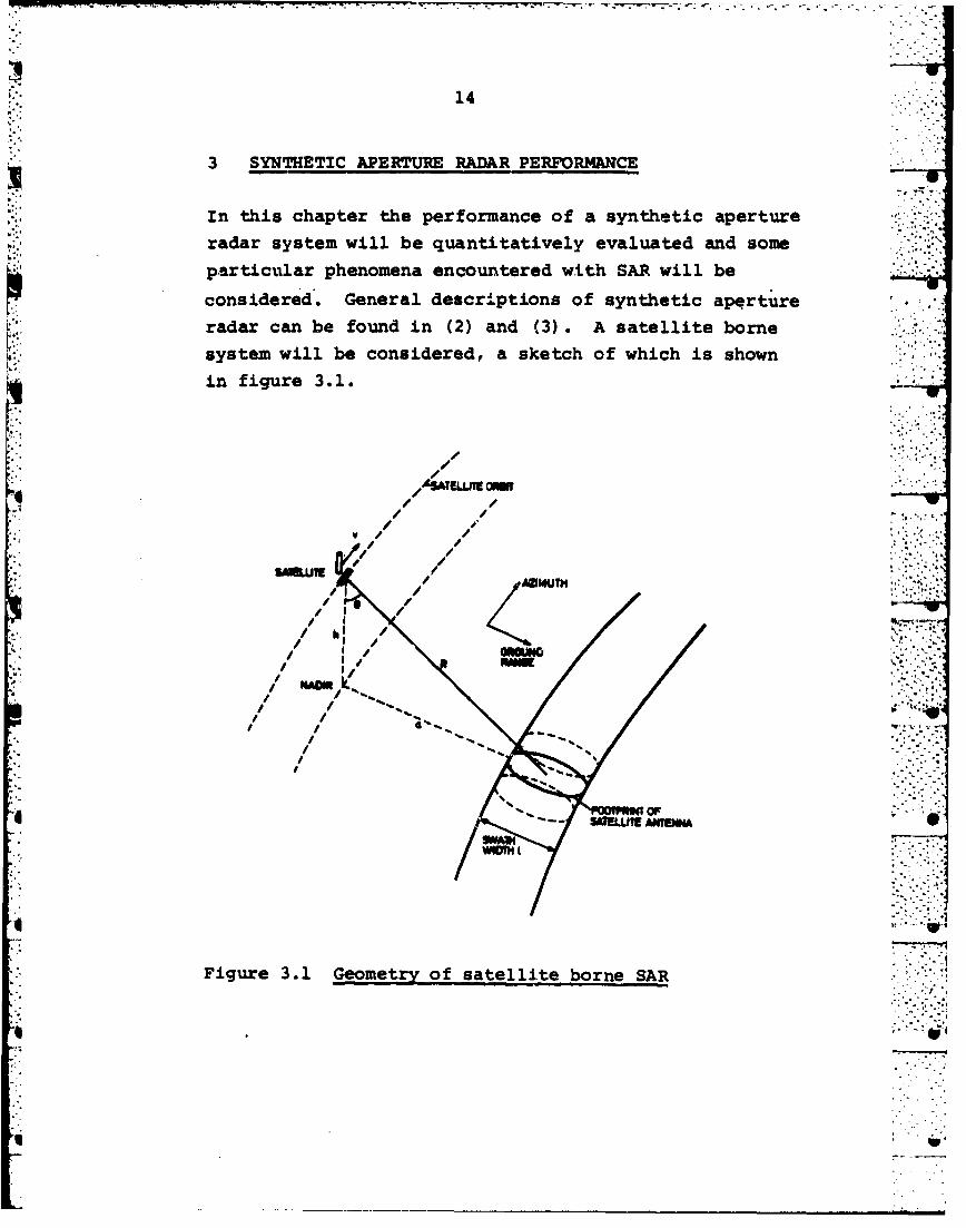
3 SYNTHETIC APERTURE RADAR PERFORMANCE-

in this chapter the performance of a synthetic aperture

radar system will be quantitatively evaluated and some

particular phenomena encountered with SAR will be

considered. General descri-ptions of synthetic apert~ureradar can be found in (2) and (3). A satellite bornesystem will be considered, a sketch of which is shown

in figure 3.1.

Ir-7

Ifn

Figre .1 eomt~yofsatllie brneS/

15 .. .,.

Approximate values for SEASAT-. are as follows:

h 800 km

R" 85) km

a- 240 kmI 1 CO km6 20.5°. " .;

v -7 km/sec

Antenna beamwidth in azimuth, 10Antenna beamwidth in elevation, 60

A general description of and detailed parameters for

the SEASAT-l SAR system can be found in (4).

In the following range resolution will be treated first

and then azimuth resolution.

3.1 Range resolution

Resolution in range with a synthetic aperture radar

is obtained in conventional manner. Although a focusedsystem has an inherent range resolution given by the

depth of focus, this resolution is highly inferior, aswill be shown later. The range resolution is therefore

obtained by pulsed operation of the radar. This is .-•-T•1+

shown in figure 3.2 where the flight direction is into

the paper.

If the transmitted pulse bandwidth is B, then the

resolution in radial direction from the antenna is

given by

&R M+"

-o*, , .. n n* -.-.,.-.lO. .... --,.'.16

*! \U 4'

hg

K \IR -- ANSI1TT. PULSE

fv i'• mI

Figure 3.2 Principle of range resolution

where c is the velocity of light. This formula isvalid also when pulse compression techniques are used(5). The corresponding ground resolution is -.

ARAR a

For SEASAT-l a linear FM-pulse is transmitted, which"gives true range 3 dB resolution AR - 7.1 m, where true

range is the distance between antenna and target. '..--"Ground range is the distance from the nadir line tothe target measured on the ground, For SEASAT-l we

have approximately 170 < e < 240, which gives therelationship shown in figure 3.3 between R and 6. The

-lower abscissa axis shows the corresponding groundrange when the satellite's height h - 800 km. 77_

From figure 3.3 it is seen that a processed SJR-*imagethat is linear in true range will be distorted in sucha way that targets on the ground at near range vii'l

"be compressed relative to ground targets at kar range.

r.-- --- ~~,~ -~- .r. .7~'~ - V - -. I - S - ' -I . -7 K . -

17

22

20s~t) ex*jk -T,

44 ~~ o Figuec 3.3 Grounde resolution. as e a ifnctiontofneoundrs

pulsuenhcy caf be isrivten onth compex formvtv as

f (t) j~k~l -T7tTkt

The carrwierh is reoe fM o i (t abvesicuisde

nTh affseect he rilnoeang resluon Thepinsanoftaneo

frequncyitof pult) iscgiven by the timetderivativeno

btheen badithe oftsnntais the agtswshimoe

18

dopplershift on the pulse echo. Figure 3.4 shows a3 ocalled squinted system where the boresight direction.mkes an angle 8s with the direction normal to the"flight direction.

I~ t~j~

Figure 3.4 Geometry of a squinted system

Vr -...s.n e .+7

"i"ssevha h rae t doTAlrsit ocur "wh.'-n

echo"o is

u~t) - s~ 2rt. 1 -,2.; 2 Vr-,

the tarerm -ivs o the phasofhemoduatio use shwhni

figure 3.4 Ate ethic apoin nter trelbtiet isesta

fit a s l pt use -eh sto m onperetw targe t is ntherge fore r ov he e. Thi g es shown in fgr-4--pl

,.t- ,.. V ,-WThe trmI - go+vest the phastne moultween usred whnd .-genertinnafo the asyteti shoneirfiure, 3b4t ith is uloset"'n"t

fo igeplecho fro one taret Ii

thrf orr removged pulse .ec h is givoestre.I s.,

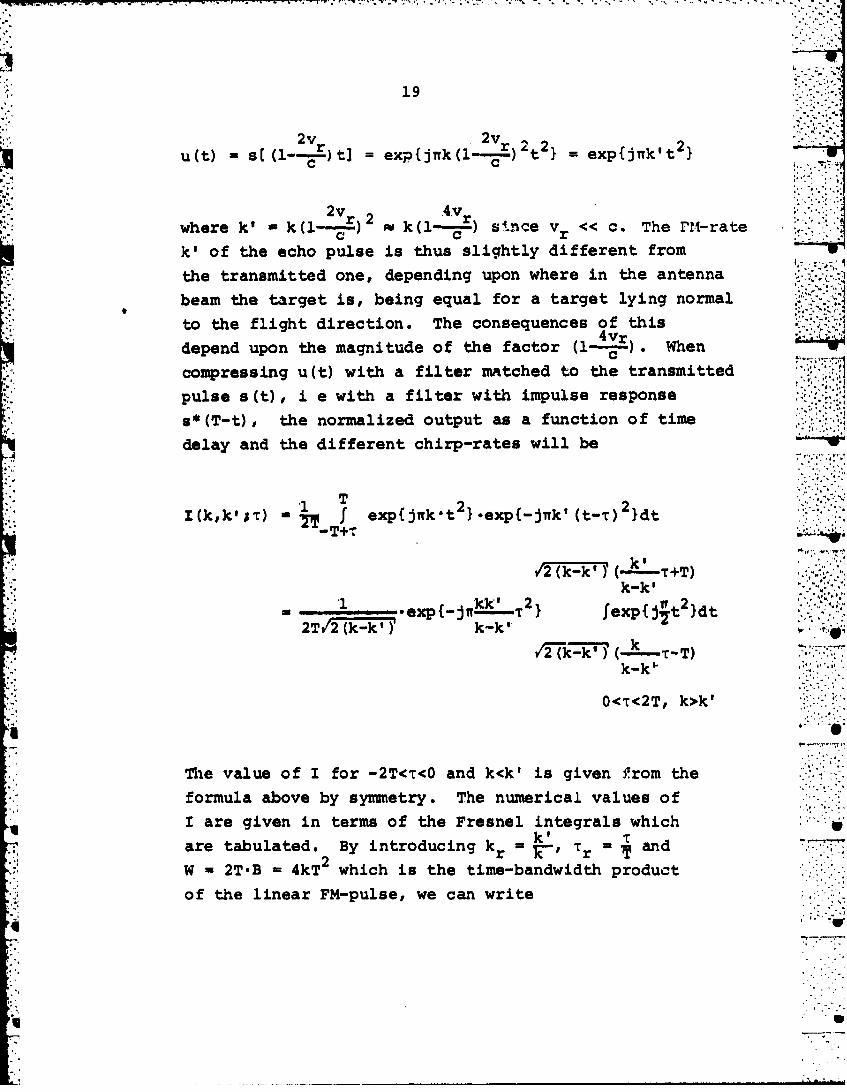
19

2v V2

u (t exp{jTwk(l-) I exp{jnk' t2}

r 2 v2 rvwhere k' k(l--) k k(1-c)sneV .TeF1rt

k' of the echo pulse is thus slightly different from

the transmitted one,, depending upon where in the antenna

beam the target is, being equal for a target lying normaltotefih0ieto.Tecneune fti

depend upon the magnitude of the factor (I----). Whento te fightdirctio. Te coseqence ofthi

compressing u (t) with a filter matched to the transmitted

pulse 8(t),. i e with a filter with impulse response

.* (T-t), the normalized output as a function of time

delay and the different chirp-rates will be *.T .

T2l~kk~sT f exp{jwrk t 2 } .exp{-Jnk'~- ) d

'2 (kk')I

*lkk' 2 Tr2 ..

= ~*exp{-JTIr-- T fexp{j t Idt *

2Tv(2(k-kk-k'

k-k"

O'cr<2T, k>k'

The value of I for -2T'cT<O and kck' is given from the

formula above by symmetry. The numerical values of

I are given in terms of the Fresnel integrals which

7-,are tabulated. By introducing -r T' r an

W - 2T"B - k hc stetime-bandwidth productof the linear FM-pulse, we can write * ~

20

I~~kri~~1-k- r +_____ T epjt

r

rok Trw 2av

sin~ii/W ((-I T),r r (32

lf~~Tr

For SkAAT1 we have W-64 Il~)Ii hr~

0< - 2" (3.2

r v -l 4ve

Thegmaimude squint aepngle for aSeAcT-l is- mapprximtel

1howhic together whith giea th relandnsi bewe th10nsies

kr 4v a25.

k (l

.Z4

0.26

Q6 To

0.29.

01O 0.9" 0065 0.002 00910 'kr

Figure 3.5 Taimem rsoutunfsepeso forlterecl matheTurem. i3Fon filrterm'ma

*4 22~4

This is seen from figure 3.6 to have negligible effect

on the range compression. If a 1 dB degradation is

set as a limit, this corresponds to kr - 0.9968, which

means that the FM-rate has to be known to 3 decimals.

Cap

Another mismatch occurs because of the carrier wave

used when transmitting the pulses. Because of the

relative velocity vr between antenna and target, the2vr

carrier wave will be dopplershifted an amount---f,

where f is the carrier frequency. The maximum doppler-4 '-

shift for SEASAT-l is approximately 1.5 kHz. This will

shift the echo pulse slightly out of the matched filter

be.ndwidth. Relative to the total bandwidth of 19 MHz1.5 kHz , .....

this is k - 7.9.10 and since the output will

be reduced with the same relative amount, it is

totally negligible.

Since the effects of relative motion between antenna

and targets are negligible, the range compression will .'-•-

be totally azimuth independent, and can be done

independently of the azimuth compression. '2'

j.2 Azimuth resolution .4..,'

The basis for generating a synthetic array antenna is

a measure of the distance between the physical antenna.

and the target as a function of time. Since this time

history is different for targets at different azimuth

positions, they may be resolved by subsequent processing

of the recorded time histories. Figure 3.7 shows the

physical configuration with a single target. -.*.-

The position vectors as functions of time, measured

from an arbitrary reference point, are xa(t) for the

antenna and xt(t) for the target. If the antenna -

23

."j.

-'I, TANSETON TM ORO=N

/RAR RVRC POW

51,*.,

Figure 3.7 Phys~ical configuration with radar and asingle target

transmits a continuous monochromatic wave a (t), wehave on comoplex form

s(t) -exp{J2lTft}

where f is the frequency of the transmitted wave. The

wave scattered from the target will be .. ,

ul(t) =exp{j21Tf[t-.ZIx-t(t)4ax(t)I]} exp ji2 nf Ct--I2 (t)IJ

If u (t) is coherently demodulated with the transmitted

wave, we, get

u(t) u u(t) *exp{-.j2wrft} ex=j-lxtl

4 ~~~~where the transmitted wavelength is X c. .....................................of the distance between antenna and target is thus done ..

as a phase measurement# or equally as a time delaymeasurement.

24

if the relative movement between antenna ani target is

linear, we have the case shown in figure 3.0, where

the target is fixed in space, and the antenna moves S..

with velocity v.

tj~

ARM?,

72--.. I

x~) r() I R4+.

Sigurde 3.the sca antenna iem nd linear b ftoundfo

finur ths.as8w. hv

25

R eReo a oa

T, - -- tan(~--+8s) Tan +

When e and e5 are small, and R0 >> vT ,vT2,w a

use the followying approximations

tanx mx and (1+x) 1+t- when x<l

We then have

u~)=4 Tt vt 2 V t2 0 uU~) exp{-j. (R0 +-) C-exp{-j27T 1-, C exp{-j-~- 2

0 0

T <t<T2 T1 +0~

R eaT=--2 (-.--+e )

The factor C in u(t) is a constant !~or a given target

and is of no importance when generating the synthetic

aperture.

Since a linear FM-pulse with chirprate k can be written

* exp{-jitkt 'I, it is seen that the phase history u(IL) for

a single target can be approxi~mated with a l inear

FM-pulse with chirprate k Th feuec bna 0 h rqunybnactually recorded is given by T? and T2 above.

1

The azimuth history can also be thought of as the

doppler history of the target as it passes through *

the antenna beam, since the instantaneous frequency

A in the azimuth history is equal to the doppler shift

caused by the relative 'motion between antenna and

target.

- . - , -- . .!.

26

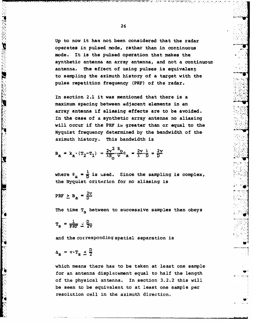
Up to now it has not been considered that the radar

operates in pulsed mode, rather than in continuousmode. It is the pulsed operation that makes thesynthetic antenna an array antenna, and not a continuous

antenna. The effect of using pulses is equivalent

to sampling the azimuth history of a target with the - -.pulse repetition frequency (PRF) of the radar.

In section 2.1 it was mentioned that there is amaximum spacing between adjacent elements in anarray antenna if aliasing effects are to be avoided.

In the case of a synthetic array antenna no aliasingwill occur if the PRF ih greater than or equal to the

Nyquist frequency determined by the bandwidth of the

azimuth history. This bandwidth is

2 R2v o 2v X 2vBa a (T 2 -TI) Ro= a - '•5=

where ea - is used. Since the sampling is complex, ---

the Nyquist criterion for no aliasing is

PRP>B 2vPRF >" Ba 2• - i'

-aD

The time T between to successive samples then obeysS

1 ,D

and the corresponding spatial separation isw

DAs -v.Ts_

which means there has to be taken at least one samplefor an antenna displacement equal to half the lengthof the physical antenna. In section 3.2.2 this will

be seen to be equivalent to at least one sample perresolution cell in the azimuth direction.

* .4

27

The effect of undersampling is that each point target

will occur in the image for a series of differentazimuth positions instead of one.

The synthetic aperture is generated by compression ofthe azimuth history, in a way similar to the compressionin range. Depending upon the complexity of thecompression filter, one can discern between unfocused

and focused synthetic aperture radar.

* '3.2.1 Unfocused synthetic aperture

The azimuth history for a target was shown above tobe given approximately by a linear FM-pulse

v 2 t 2

(t- exp{-j2..°} , TI<t<T2.9 0

An unfocused synthetic aperture is generated by

compressing u(t) with a filter that has no phasecorrections. If the length of the synthetic aperturemeasured in time units is tul the azimuth pointrespornse is given by

t4t , u,

a(t)= f u(T)d-r

t4

It can be shown that minimum angular 3 dB resolutionoccurs when tu = 1.2 .t 1 , where tI is defined by

2 2t 1 0

2w t

28

Figure 3.9 shows a target and a spherical wavefront

emanating from it. Generation of an unfocused

synthetic aperture corresponds to integrating the

incoming wavefront over an area where the wavefront

can be regarded as approximately plane.

WAVIVRNT :'.

LoWN O - - - - -- - -- - - -- .- - - --- - - - - --- :'*AO

OuO

SYWIHEIKAPMRURE

Figure 3.9 Generation of unfocused synthetic aperture

To find the resolution obtainable with unfocused '.

processing, we assume an allowable phase difference

from center to edge of the antenna of •, as was used

in section 2.3 to find the boundary between the

Fresnel and Fraunhofer regions. From section 2.3 we

then have

".~~ I Du M.,-R.'.

0

The ground resolution obtained can be found by considering

the bandwidth of the azimuth history along the synthetic :-

aperture. This bandwidth is

=L~'2v 2v"BU =tuka v "ki o _.

-. .2s~~v.*~..>wvxr ;--.T- - - . -

29

Ground resolution is then

lop

U

The antenna diagram for unfocused processing is given

by the point response ,

a~t) f u(t)dt -f ex{-j2n=V}dTt t 0

Up -

This can be evaluated in terms of Fresnel integrals.

The antenna pattern in angle can be found by settinge -for small values of e. Figure 3.10 shows a(t)

for different values of t 1 the length of the

synthetic aperture in the time domain. t1 ~ is * -

used as a parameter.

1-0 SY16VR NTHETIC APERTURE LENGTH Luxv-tu

0.u06 A

0.2-

a S0.5 1.0 1.5 2.0

Figure 3.10 Antenna diagrams for different lengths ofthe unfocused synthetic aperture

30

3.2.2 Focused synthetic aperture

In section 2.3 it was shown that the need to focus an

antenna only arises when the target is in the Fresnel

region of the antenna. The target is said to be in the

Frasnel region when the distance between antenna and'D2

target is less than 7-, where D is the length ot the

aperture. For SEASAT-I we have X - 0.24 m and typicallyI, .'

D o 4 km, which gives - 65000 km. Since the actual

distance between target and antenna is approximately

850 km, all targets are seen to be deep in the Fresnel,

region of the synthetic antenna.

1',:4 With focused processing the received wavefront is phasecompensated aci'oss the whole synthetic aperture. This ,is equivalent to matched filtering of the target's

azimuth history. In this case the complete azimuthhistory is compressed, and the bandwidth was earlier

found to be

B- 2v

This gives ground resolution

V D',:.-f

The reason for the range independence of the azimuth

. resolution is Lhat while the azimuth bandwidth isrange indepe-adent, the time it takes for a given targetto pass through the beam of the physical antenna is

proportional with range. The time-bandwidth product of

the azimuth history is therefore proportional with ".9

range, and the azimuth resolution remains constant.

*. Since the azimuth history is a linear FM-pulse, theperformance of the azimuth compressi.on is expressed

by formula (3.1). The time-bandwidifh product of the

I I II II I I

31

"complete azimuth history for SEASAT-I is approximately3200. The azimuth antenna diagram without weighting

and with perfect focusing is given by (3.2) withW - 3200. An actual antenna diagram with weighting

is shown in figure 4.15.

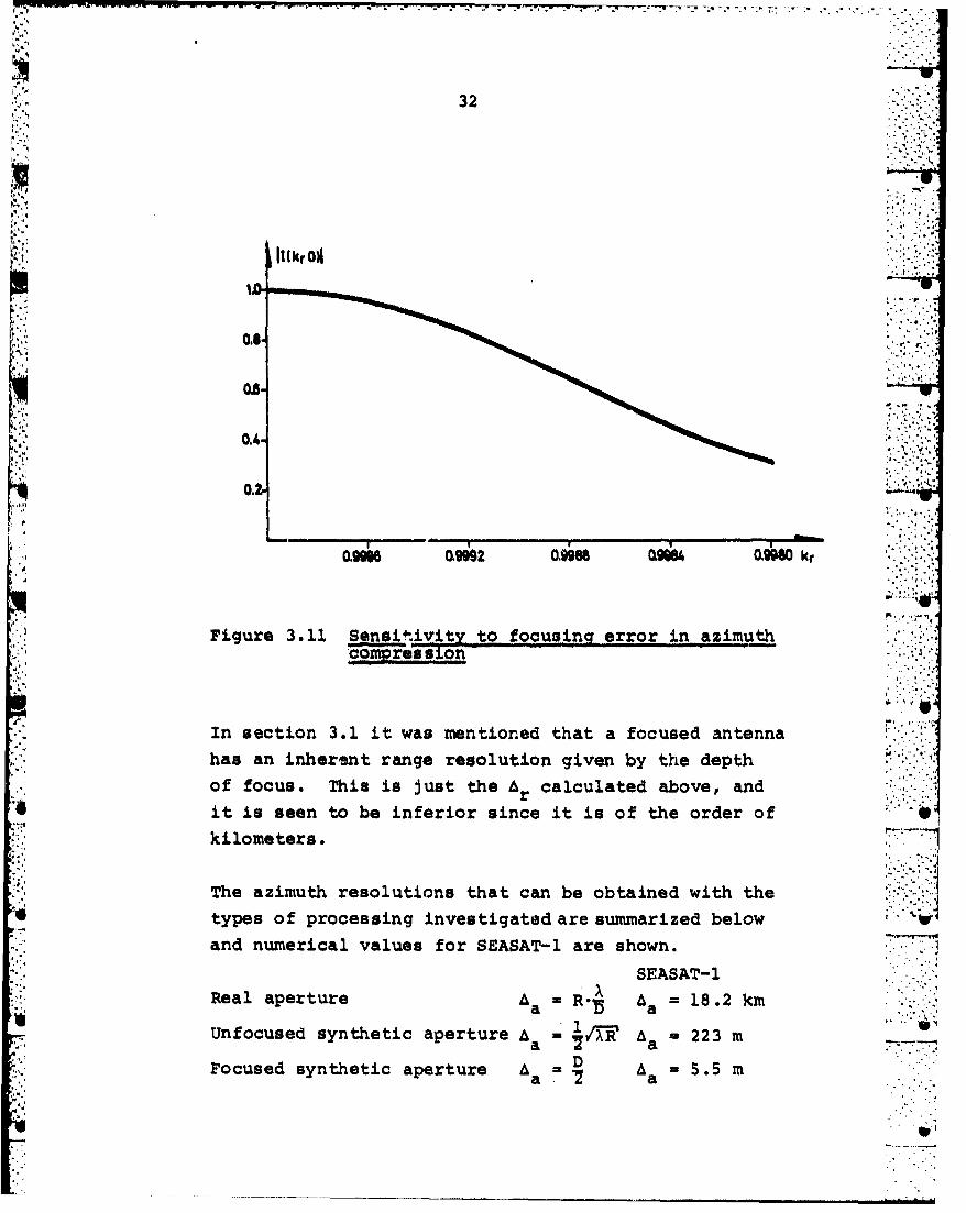
The effect of a focusing error is given by lI(krr,0)."and is shown in figure 3.11 for W - 3200. If anazimuth filter matched to targets at range RO is used ,.

also for targets at range RI, RI<R0 , this correspondsto a focusing mismatch

2v 2 2v2,•kr �o,-*I uR1krRO

•~R R,".:0 1

From fi r ua 3.11 3 dB degradation is found to givekr - 00.98-. With Ro - 850 km we have R, - 849.065 km.

This means that the true range interval over whichthe same azimth filter can be used if 3 dB degradation

is tolerated at the edges, is

Ar - 2(Ro-RI) - 1870 m

The corresponding interval for 1 dB degradation isAr 1105 m.

r6

In section 3.4 it will be shown that the normal

processing mode does not compress the whole azimuth

"history coherently. If shorter parts of the azimuth

history are compressed coherently and afterwardsincoherently summed, aach part will be less sensitive ,

"to focusing errors because of the lower time-bandwidthproducts. The case evaluated numerically above can

therefore be regarded as a worst case.

t U

32

016r.• ii; : :

"' ~~~~0.4. ";-.:-

0.20 •i

0.9096 0.9992 0,9986 094 0.9080 kr

Figure 3.11 Sensitivity to focusinq error in azimuthoom2rem sion

; *.. ,. 0,**

In section 3.1 it was mentioned that a focused antenna

has an inherent range resolution given by the depthof focus. This is just the Ar calculated above, andit is seen to be inferior since it is of the order of "

kilometers.

The azimuth resolutions that can be obtained with the *types of processing investigated are summarized belowand numerical values for SEASAT-l are shown.

SEASAT-IReal aperture Aa = R A = 18.2 km

a AaUnfocused synthetic aperture A =.1/XT A = 2 2 3 m

Focused synthetic aperture a = D A - 5.5 ma. a

44.

33

3.3 Image distortions and artifacts

There are different kinds of distortions that appear

in a synthetic aperture radar image of an area onHi. the ground. These can be divided into deterministic

and stochastic distortions, although the distinction

K between these two is partly a matter of definition,

The simplest type of distortion is the purely geometric

distortion which gives a scale distortion, in generalnonlinear, of the image. This kind of distortion wasmentioned in section 3.1, where the difference betweenground range and true range was treated. Similar

distortions may also occur in the azimuth coordinate

depending upon how the azimuth filters are generated.This is a correctable distortion, since it only uausesa warping of the coordinate system in the processedimage. It will not be treated here, since the absolute

locations of targets in an image is of little

importance for the purposes considered here.

First a type of distortion called range fold-over is

treated. Then imaging of moving targets is studied.

At last stochastic errors are briefly considered.

3.3.1 Range fold-over

Range fold-over is a distortion that stems from the '.1difference between true range and ground range.Figure 3.12 shows a mountain and the way it will"appear in the image.

All the three points A, B and C are at the same truerange from the radar and will therefore be mapped to

the same image point. This has the effect of folding

the mountains towards the radar.: ::'::

-, .. . -- - . - ,. '. • ,.j

................- K

34

U -V'":

: ,t, ,-. '.

TMAIN

9' I ORUNO PA=S

Figure 3.12 Example of range 'fold-over

The displacement for an object at height h from its ,dJ

correct ground range position is approximately, from

figure 3.12,

6- h-cotane for SEASAT-I ar o h'cotan200 w 2.7 hrI

This type of distortion is incorrectable and is easily

seen in images of mountainous areas, as for example in

figure 4.22.

3.3.2 Moving targets

* As shown earlier, the principle of generating a synthetic

aperture is based on relative movem'ent between target

and radar platform. When imaging the surface of the

earth, a target that is in motion relative to the surface

will be imaged differently from a target that is

fixed on the surface. This will. for exarple be the

case for a moving ship, and even for the soa itself

although the motion of the sea surface to a high degree .

may be considered as stochastic.

35

It was shown in section 3.1 that the dopplershift caused

by a moving target is of no concern in range compression...

The only effect of a moving target therefore appears in

the azimuth compression.

It was shown in section 3.2 that the recorded phase

history for a target is

u(t) -- "(t) TI<t<T2

41

where r(t) is the relative displacement vector between

antenna and target. For quasi-linear relative motionwe have

(t)I (R 2V 2.

It is convenient to divide the target motion intocomponents in range direction and azimuth direction. e

There will also be a component normal to both therange and azimuth directions, but this can be neglected

for all targets of interest.

If terms of higher order than second are neglected,the motion of a target relative to the ground in thecoordinates mentioned above can be described by fourparameters, vr, va, ar and aa, where v is velocity and

a acceleration, and the indices are r for range and afor azimuth. The length of the displacement vectorfor a moving target can then be written

1 22j[(t) I = {[Ro+vr" t+'art ] +[(v+va) t4taat I

"By retaining terms up to second order in time, we get

(,v+v 2 .Ir~t a Rovr a

V

36

The corresponding phase history is • *, "..

2

We see that with the approximations made here, the

acceleration aa in the azimuth direction has no impact

on the processing.

The difference in phase history between a moving target

and a stationary target is

where the approximation 2vv+ 2v~va has been used..."°

ar{ a a~2

since v>>Va. .',".

The term vr. t represents a frequency shift in the,:,,,.:.•'.

azimuth history of -- ',- Hz. Since the azimuth history *-*.*,;.

of a target is approximately a linear FM-pulse, thised

means that the effect of the velocity component vr •'•

is a displacement of the target in the processed.,..' ,,image in azimuth direction.

The effect of ar and va is to change the chirprateof the azimuth history. z neThe chirprate for a h

stationary target is hpr mt , and for a lmving ,,...,,..target we get chirprate ,-gt.'t'p'cse

('1 a V 7a) .,' 7 T. ,:-

Expressed in relative terms we have the cra

or a -"

kr~ =~ = (R-aY 2v +)- -

The effect of this mismatch is to cause defocusing

of the target in the image. -

Lu ___________________________________0

* * -4. - *. -~ .. ..- •-. -'.4...

37

The velocity component vr may also have another

impact on the processing since it changes the target

trajectory in the raw data. Since the trajectory is

oriented mostly in the azimuth direction, it is very

little sensitive to v. The change in trajectory will

cause a smear of the target in the image. ,

The extra range migration for a moving target during

the generation of the synthetic aperture is

yr R•X r ov0

where D is the length of the real anteanna. T is

the length of the synthetic aperture.

The quantitative effects of thesi6 distortions are given

below in terms of numerical values for SEASAT-1.

The dopplershift in the azimuth history dye to the

radial velocity vr was above found tobe- Hz, where

vr is positive away from the radar. The dopplersliift

caused by a stationary target as it passes through the

antenna beam is continuously decreasing. If a moving

target causes an extra dopplershift, this corresponds to

a target appearing earlier if the extra dopplershift is

negative, and to a target appearing later if the

dopplershift is positive. The displacement of the

target in the image will therefore be as shown in

figure 3.13.

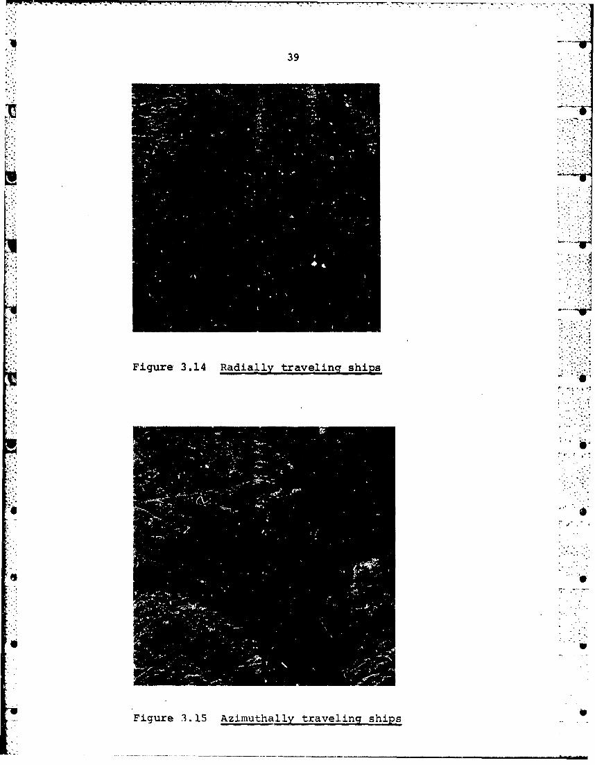
An example of this phenomenon is shown in figure 3.14,

where several ships moving in the radial direction

are shown. The wake shows the direction of the ship's U

movement and where it actually is. The azimuthal

displacement of the ships themselves is clearly seen

from the figure. In figure 3.15 ships moving in the

re

38

RADAR PLAMORM.4,

0-ACTUAL POSITIONFAG OF TAMSET

0-POSITION OF

TARGET IN IMACE

0 ~¶POSITWI

4, Figure 3.13 Displacement in image of radiallsy movirngtarget

azimuth direction are shown, and no "iisplacement from

A. the wake is seen to occur.

A displacement in azimuth with one resolution cell,

i e 25 ml gives

2vrr ~-v 25 ma

vwhere ka is the azimuth chirp rate. Typical values forSEASAT-l are ka F 500 Hz/sec and v ow 7000 m/s, and we

get

yr w 0.2 rn/s

With a depression angle of 700, the corresponding

ground range velocity is

V 9 V r/cos7O0 ow 0.65 rn/s =1.3 knots7.

"w - - Y v-r w r r- - r-w- - - --

39

ifd

Figure 3.14 Radially traveling% ships

Figure~~~ ~ ~ ~ ~ 3.5Aiuhly0rvln hp

40

Typical displacements in figure 3.14 correspond to

velocities of approximately 15 knots, which is seen

to be quite reasonable.

Smearing in the image caused by vr is said to occur

when the radial displacement turing the synthetic

aperture is greater than one range resolution cell.

This is approximately 8 m for SEASAT-1 and gives

rXRo-

v8 m

D 11 m, v -7000 m/s and R- 850 km gives

Vr > 3.1 m/s • 6 knots

Corresponding ground velocity is :..,

Vg > 18 knots

In section 3.2 it was found that a mismatch in focus

corresponding to kr = 0.9989 gives a 3 dB degradation

in peak response. It was found above that the

components a r and va give a mismatch in focus

corresponding to

Roar-r + va + -.

V -:

With R= 850 km and v =7000 m/s we have

kr = 0.9989 and ar =0 va =3.9 m/s =7.6 knots

kr = 0.9989 and va 0 - ar - 0.06 m/s 2 ag P 0.2 m/s 2

r a

-4j

41

Since an acceleration of 0.2 m/s 2 is very high for a

ship target, defocusing is likely to be due to theazimuthal velocity component va.

The numerical results derived above are summarized below. _

All velocities are ground velocities.

Azimuth displacement vr > 1.3 knots

Smearing in range vr > 18 knots

Azimuth defocusing va > 7.6 knots .aV

If the azimuthal displacement from the wake is usedto estimate the ship's radial velocity, vr - 1.3 knotscan be regarded as the velocity resolution.

3.3.3 Stochastic errors

Some of the errors can only be modelled as stochastic

errors, and the effects expressed in terms of meanvalues, variances and correlation functions. The mostimportant of this type of errors can be expressed asphase errors in the azimuth history of a target. If the

azimuth history of a target is written

u(t) a(t).exp{-j.,(t)}

where a(t) is the amplitude and 0(t) is the phase

history of a target, then a phase error 60(t) canbe included by writing

u(t) a(t).exp{-j[O(t)+6f(t)1}

Fluctuations in a(t) have been neglected since they arein general of less importance than 6ý(t). The phaseerror term 60(t) includes random propagation delay

V_'

42

through the atmosphere, phase Jitter in the applied

signals and random motions of targets and platform. The

effect of 60(t) on the compression operations will depend

upon the statistical properties of 60(t). This type of ;"

errors is not analyzed here, but references (6) and (7)

contain results from investigations of such errors.

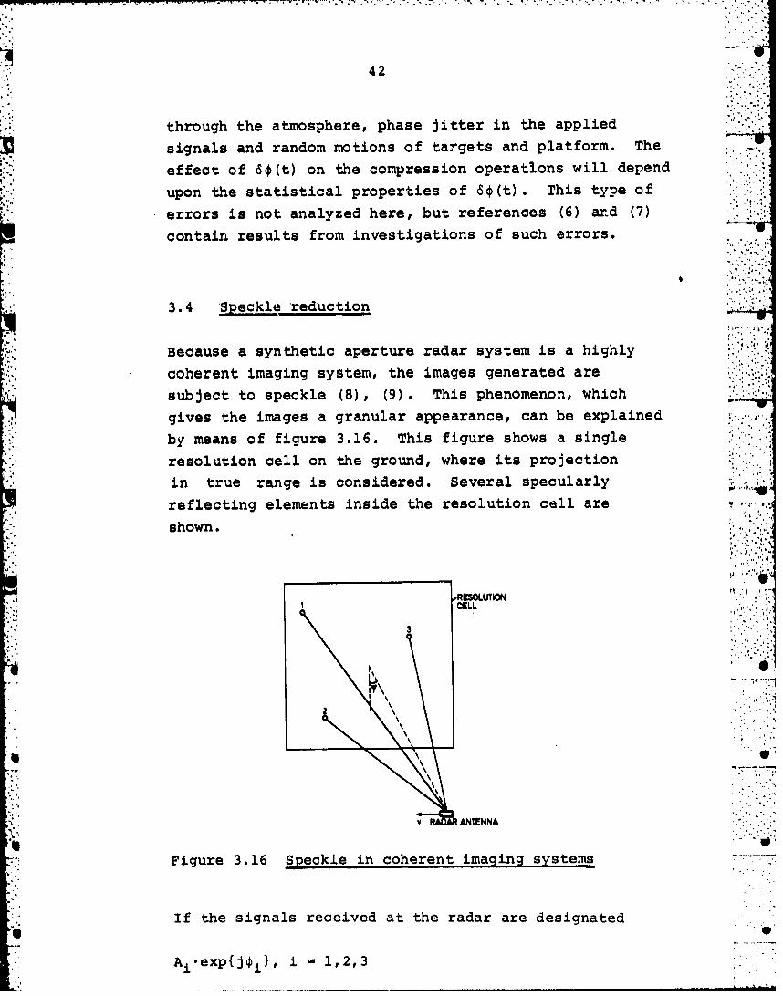
3.4 Speckle reduction

Because a synthetic aperture radar system is a highly

coherent imaging system, the images generated are

subject to speckle (8), (9). This phenomenon, which

gives the images a granular appearance, can be explained

by means of figure 3.16. This figure shows a single

resolution cell on the ground, where its projection

in true range is considered. Several specularly

reflecting elements inside the resolution cell are

shown. .

oRESOMUTIONCELL

5. ~3j

S-

vRADAR ANTENNA

Figure 3.16 Speckle in coherent imaging systems

If the signals received at the radar are designated

Ai.exp{joi}, i = 1,2,3

-~ 43

where 0i includes both propagation delay and theinternal phase of the scattering elements, the complexamplitude at the receiver will be

3a () Z A -exp(Joi}."-•'-

where the dependency upon the viewing angle 4 has been

explicitly denoted. i has a one-to-one correspondencewith the azimuth time coordinate, and the received

signal is therefore seen to vary in time in a mannerdetermined by the spatial locations of the scatteringelements inside the resolution cell.

In the general case with N scattering elements inside

the resolution cell the received signal will be

Na(} E A .i exp{jii}

•' ~~~and both Ai and Oi, and consequently a(*)# can be '.:,:?regarded as random variables.

If all the Ai's and Oi's are statistically independentand the Is are uniformly distributed on the interval

* (-[-,,t], the addition of the complex amplitudes at the

receiver can be regarded as a random walk in the complex - "plane (9). If the number N of scattering elements ishigh, this process is similar to the narrowband noiseprocess, and the probability distribution of la('!•) I is

equivalent to the distribution of the amplitude ofnarrowband noise, i e the Rayleigh distribution. We

thus have

p(jaI) 2 exp- , a>0a a0 0

44

where ao <la2> 12P0

The intensity of the received signal .Ls I(t)= Ia(*) 2,the distribution of which is exponei-i .lai..

p(I) Y - exp{-r } (3.3)0 0

where 1 - <i> is the expected value of the intensity.

The geometry shown in figure 3.16 is not directly

applicable to the case of synthetic aperture radar,since each resolution cell is imaged by means of asynthetic aperture extending over an interval of theviewing angle . If, however, this imaging process isthought to ocuur separately for each scattering elementinside the resolution cell, the resulting signal can be -,r

assigned for example to t~ip! midvalue of the ýp-interval,and the geometry will bL "pplicable also to the SAR"

case .

The assumptions about the statistical properties of ,the scattering elements, which are characteristic of

what is called fully developed speckle, can not beexpected to hold for very strong targets, as forexample urban areas on land and ships on the sea.For most land areas and for the sea surface, however,the aasumptions will in general be well satisfied. Aresolution cell of 25mx25m on the sea surface will

contain many independent scattering elements, and witha radar wavelength of 23.5 cm the phase execursions over

the resolution cell will be large enough to give uniformphase distribution.

• , , - ,

An example of an image of a sea area is shown in

figure 3.17, where the speckly nature of the ,Lmae"clearly can be seen. Figure 3.18 shows the probability

distribution function of the intensity calculatedfrom the image and also the theoretical distributionaccording to formula (3.3) where the mean intensitycalculated from the image has been used. They ireseen to be in excellent agreement with each ohter.

, o ,' 1'(

Figure 3.17 Image of sea area showing speckle

As mentioned above the speckle in the images is catiedby the coherence of the imaging process. The speckleeffect can be reduced if several uncorrelated images-ofthe same ground area are generated and afterwardsincoherently added, that is added on an intensity basis.

The contrast of a speckle pattern is defined as

C -(3.4)0

46

THEORETICAL DISTRIBUTION 15 FULLY DRAWNDOM ARE MLLE" "ALAW FROM, IM, '

744 174

ma ,l of ,h it W.i

Fiue318d~4yistribution fivr iman (33 egtC-1 diion

tw erthegoratiolbetweeathen standarddeviatio ad thaes

imaean valudo the intenusity Weeith tohenprbateimaits

Tefrormua aboveen parts ofo thesigarle speckle. Thys uinage

will be uncorrelated if they occupy nonoverlapping* parts of the spectrum. This method represents a

compromise between resolution and speckle reduction.

4.",•'i

," .- 4 -. ,...- *-.*-

47

i The t-vodimensional signal spectrum is shown in figure3.19, where it is divided into Nr equal frequency bands

K..: in range and Na bands; in azimuth.- .. .. ,-,4

No

.4' 1A~RANSE-.

4rnigur 3.19 Division of signal spectrum in equalfeuenc") bandis

:o. :.£

This will give Nr N a uncorrelated images. If the bestresolutions that can be obtained by the system are Arin range and Aa in azimuth, which corresponds to NrN a f , this procedure gives resolutions Nr Ar andNa&Aat and a speckle contrast I//Nr.Na'

In the case of SEASAT-I we use Nr 1 and Na -4. This "'T72gives a resultin.g ground resolution of approximately25mx25m and a speckle contrast of 0.5. Since the

Sazimuth history is a linear FM-pulse, the different ,". WN

frequency bands correspond to different time sectionsas shown in figure 3.20.

Each of the sections is called a "look". Since each '•4look represents a particular viewing angle, uncorrelated

images are seen to be obtained by angular diversity.

48.-1N

IMOIT

ARANDE-/I - /~ I U

' ,. . , ,

/ / I S

Allm

I./ LOOK / 2.LOOK i. .L.K

TOTAL UYNHETIC APERUME 9

FLIGHT DIMOCTION

Figure 3.20 Generation of 4 uncorrelated looks

"Partially overlapping looks will give a look correlation

that depends upon the degree of overlap. The images

processed here have the four looks placed in the time

".4 domain as shown in figure 3.21.

.,LOOK 2. LOOK 3 LOOK 4. L•OK

- TOTA'L SYNTHET!C APERTURE•;,"1. 71 ,,

'Figure 3.21 Four partially overlapping looks

"The window functions used for the looks are shown, and

neighbouring looks have 1/3 overlap on the time axis.

• ' Because of the window functions, the effective overlap

49

will be less than 1/3. The lowest curve in figure4.25 shows that a contrast of very nearly 0.5 is

obtained in this way for a sea area, which shows thatthe 4 looks are nearly uncorrelated.

Figure 3.22 shows the four different looka for an areain the Strait of Dover, and figure 3.23 shows the effect. .....

when adding the looks together. The reduction in

speckle when averaging looks is easily seen.

--- -------.

•.• I ;, +

"A...%%• +

0''" ''•.

* , .:4' "

1"" "

-q.. . +

r; ,

I,;/..'• +

",I.';,'

50

44 .

First look Second look "

1.410

ThirdlookFourt loo

Fiur 3.2 Fordfeen4ok4fth aeae

1 lok lok

3 looks 4 looks

Fiur 3.2 Efeto oo vrgn

52

4 PROCESSING OF SYNTHETIC APERTURE RADAR IMAGES ..

Processing of SAR images from rawdata consists ofmatched filtering of the rawdata with a filter

matched to the point target response. This is atwodimensional filtering operation in range andazimuth.

When generating a SAR image, the last operation is

conversion from complex amplitude representation ofthe signals to intensity. Although this is a

nonlinear operation, the quality of the image is Iwell described by signal to noise ratios before

intensity conversion because all the precedingoperations are linear filtering operations.

The received power can be found from the radarequation. If the scattering cross section of a

resolution cell on the ground is A.o, where A isthe area of the resolution cell and a is the radar

0N

reflectivity, the received power isPt .G2 "\ 2 .A.a• 5"••

=t 0Pr = 3 R4 •"'(4 it) *R

where P t is transmitted power and G is antenna gain. 'The system noise power is

N - kTB

where k is Bolzmann's constant, T is effectivenoise ".temperature and B is receiver bandwidth. For SEASAT-1

we have

Pt = 800 W

G = 35 dB

T = 650 K

B = 19.106 Hz

R =850 km

53

2For 1 look and full resolution we have A m 150 m which

gives signal to noise ratio

G2 2 :.."P- P = 3.8-10-.ao = -34 dB+ ao[dB]N (4) 3 . R4 0k.T.B

For an average sea model we have in the middle of the

swath (4), a0 = -14 dB which gives

-= 34 dB -14 dB -- 48 dB

The processing gain is given by the time-bandwidthproducts of the range and azimuth waveforms, 634 inrange and approximately 3200 in azimuth. Processing

gain is then

Gp 634 3200 2 .03106 -63 dB

This gives a resulting signal to noise ratio of

"63 dB 48 dB =15 dB.

Processing of SAR images has in the past mainly been -;

done by optical processing, where a configuration oflenses ane a coherent light source are employed. The

rawdata signal is stored on film in a twodimensionalformat, the optical system scans this input film andthe output is images which also are recorded on film.

The main reasons for doing the processing opticallyare processing speed, t-he suitability of film as astorage medium for lc.,rge amounts of rawdata, and thefact that the azimu-'" signal for a target, used for

generation of the synthetic aperture, exhibits self

focusing properties in a coherent optical system.

54

Descriptions of signal formats and optical configurationsused for optical processing of SAR images can be found

in (10) and (11).

4.1 Digital processing

Although optical processing of SAR images still is

used when really great throughput is needed, digitalprocessing has some important advantages. The optical

configuration needed is not very mobile and the optical

recorder needed for recording the rawdata signal onfilm is a critical element. These are avoided with

digital processing, and the ease with which processingparameters can be adjusted and optimized in digital.

processing tends to give digitally processed images

"higher quality than optically processed ones.

The SAR in SEASAT-l was an L-band radar operating at

1.275 GHz. The pulse echoes were upconverted, to S-band

before transmission to ground. After reception onthe ground the echoes were demodulated and convertedto 5 bit samples and stored on magnetic tape.

The data recording is a twodimensional samplingoperation, sampling in azimuth by transmission of

pulses and in range by the A/D-conversion mentionedabove. The sampling frequency depends upon whether

the sampling is real or complex. If the azimuthsampling is complex, this gives a PRF that is only

half the corresponding real sampling frequency, andit also makes it possible to use a recording window

that has the double length of what it has in the caseof real sampling. For SEASAT-l the sampling iscomplex. An explanation of differences between these

modes of operation can be found in (12).

55

The twodimensional filtering that has to be

accomplished is performed digitally by do4ir ti-w.onedimensional filtering operations, one In range

and one in azimuth.

It is convenient to consider the recorded radar

echoes as a twodimensional signal, and in the caseof optical processing this is actually done when

recording the signal on film. A similar format whenusing digital processing is shown in figure 4.1.

AMMUTH

'I .. , ". ",,

• S • ' " '

-*Figure 4.1 Twodimensional digital data format

The dots represent the recorded samples, i e one

vertical line represents one sampled pulse echo.

The area A shows how the echo from a single target

is distributed in the recorded data when the radar

antenna is pointing directly normal to the direction

of relative motion between target and antenna. The

distribution of the target history in range is

caused by the length of the transmitted pulse, and

the distribution in azimuth represents the synthetic

aperture.

vertcallinerepesens oe saple pule eho• •"":-w

56

B is the target history for a squinted system andrepresents the typical target history with SEASAT-l.

The processing of a SAR-image from rawdata means

to compress the target history in both range and

azimuth to an extension equal to approximately one

sample in both directions.

While the range compression is strictly onedimensional

and, as 3hown in section 3.1, completely azimuth

"independent, the azimuth history is curved in therange direction, socalled range migration, and it

is also range dependent. In the next two sections

range and azimuth compression will be treated separately.

A block diagram of the processor is shown in figure

4.2.

Figure 4.2 Block diagram of digital processor

After a suitable block of rawdata has been written todisc, the doppler centroid in the azimuth spectrum is

estimated. The estimation algorithm is very r imple

and it is briefly explained in Appendix A. When theK. ~doppler centroid is estimated,, a block of rawdata is 4-

compressed in range, and an interpolation is performed

for each range compressed vector before it is writtenback to disc.

"57

Since disc is a onedimensional storage medium, therange compressed datablock has to be transposed, or V

corner turned, before it can be accessed in the

azimuth direction. This corner turning is doneeffectively by means of the socalled Eklundh'salgorithm. It is explained in (13). After corner

turning the azimuth filters are generated. To

generate the correct matched filters for azimuth

compression, three parameters related to the satelliteorbit and attitude are needed. These are

1) distance between radar and target

2) effective squint angle of the system3) relative velocity between antenna and target

The two last parameters will be treated in more detail

later, but briefly it can be said that 1) is given 'V.

by the parameter called range pulse delay in figure ... 04.2, 2) is given by the doppler centroid in the . .. '..

azimuth spectrum, and 3) is estimated by the auto-

focusing procedure described in section 4.4.

During azimuth compression the four looks areseparately generated and afterwards incoherentlyadded to give the final multi-look image. .

To generate a complete image the sequence of processingsteps is repeated a number of times except the doppler ..

centroid estimation and the generation of the azimuthfilters.

The theory of linear digital filtering is describedin (14). Digital filtering can be done either inthe time or frequency domain, where frequency domain

filtering is more efficient, measured in number ofoperations, for filter lengths more than approximately

30 samples. Since the lengths of the matched filters

58

used here are typically several hundred samples, the

pulse compressions are done in the frequency domain.

Forward and inverse digital Fourier transforms (DFT)

are calculated by means of the Fast Fourier Transformalgorithm (FFT), described, in (15).

The theory of matched filtering can be found in (5).

The details of the algorithms will depend on theradar system used and the actual system parameters.

There will for example be operations that arenecessary when processing data from a satellite

borne synthetic aperture radar that would not be

necessary if the radar was airborne, and vice versa.

Although the algorithms developed here are for asatellite borne radar, they include all the principles

of the synthetic aperture radar and could, with some

modifications, be used also for airborne SAR.

A detailed description of the algorithms developed here

together with computer programs written in FORTRAN that ,....,,

implement these algorithms on a general purpose computer

are given in (16).

4.2 Range compression

During range compression each pulse echo is filteredwith a filter matched to the transmitted linear FM-

pulse. This corresponds to removing the range distri-

bution of the target history as it is shown in figure

4.2.

The analog to digital conversion of each pulse echo is

done to 5 bit real samples. During range compression

these are converted into complex samples which reduces

the sampling frequency in range with a factor 2. This ',*

59

also reduces the range migration of the target

histories with a factor 2 measured in number ofsamples. This makes the range migration correctionduring the azimuth compression easier, and it givesdirectly the phase information necessary for generating

the synthetic aperture. The real to complex conversion

is done as follows.

A DFT of a 2N-point real sequence gives a 2N-pointcomplex sequence where the upper half of the sequence

of frequency components is given as the complex

conjugate of the lower half. By discarding the upper

N complex frequency com.ponents and taking an N-point

inverse DFT (IDFT) of the rest of the sequence, an

N-point complex time sequence is obtained which

represents the complex version of the 2N real samples,

Another method for obtaining the complex samples

would be to take the Hilbert transform of the real

samples, which would then give the imaginary parts

of the complex samples.

The transmitted pulse is a linear FM-pulse with chirp-rate 5.63-1011 Hz/sec. On complex form its duration

is 768 samples, and the frequency spectrum is shown

in figure 4.3.

Figure 4.4 shows the received frequency spectrum

averaged over 100 pulse echoes.

when a suitable block of rawdata has been written to

disc and the doppler centroid has been estimated,

range compression is performed. This pulse compression

is accomplished by filtering one range vector from the

rawdata matrix at a time with a filter matched to thetransmitted pulse, and storing the undistorted output

values in matrix form on disc.Vi

60

Figure 4.3 Frequency spectrum of transmitted pulse

510 1520 t(MHZJ

V Figure 4.4 Averagedl received 'spectrum in range

61

The rawdata is packed with three 5 bit samples in a

16 bit word, and the unpacking necessary prior to

range compression is done in the same routine that

does the range compression.

Conversion from real to complex s.znples as mentionedabove, is efficiently done by utilizing an N-pointcomplex FFT routine for the transformation of 2N realsamples, and afterwards descrambling the output values

cf the FFT routine to get the N complex frequencycomponents wanted. The method is described in (15).

Figure 4.5 shows a block diagram for the range compressionroutine.

M IAC oic usg OFT N IOPI X MUIU

Figure 4.5 Block diagram for range compression

The input vector xI contains coded real 5 bit samples.x1 is decoded to the complex vector x 2 (i), i - 0,N-1,where N - 4096 is a typical length chosen as processingvector length. The consecutive real samples are

stored in Re{x 2 (O)}, Im{x 2 (o)}, Re{x 2 (I)}, Im{x 2 (I)},--.Fourier transformation gives

N-1x3 Zi) - x 2 (k).exp{-jg-i.k}, i = 0,N-1

k=o

Descranibling is done according to the following algorithm.

_ ~62 -

R_ R (-i) O- [ i) I(MRe- (N 14

-c '7Ti* R(i) -R,(N-;i) 1 ± OIN-l

where RMi Re{x3 (i)}, 1(i) l m{x3 (±))1, and x3(N x3(O)

The matched filter's frequency components H(i), i - ON-lare calculated and stored before range compression

begins. Filter multiplication gives

x 5 (i -H x i.(')1 i ON-l

The received pulse echoes have a carrier frequency .. 9"

which is half the complex sampling frequency.

Demodulation is given as

M6i N (4mdl N], i - ON-l

* Tranisformation back to the time domain'

x7i)- 1 N 2nx (ik- I x (k).exp{J~ itk}, 1 0, OW-1

Because of "wrap-around" in the filtering, the

undistorted output values are

*x 7 (i), i =O,M-l

where M =N-767, since the length of the impulse

response of the matched filter is 768 samples.

Interpolation in x 7 uses a 4-point interpolationfilter which gives

X8 (i) Z x 7 (i+k+m) 'sin' (k-l-T)(T.]I OT<l, i - 0,M-4 (4.1)

m and T vary from pulse to pulse and are determinedas explained in section 4.3. The filtered vectorx8 is then written to disc.

No weighting is applied to the range pulse to reducethe sidelobe level, and the time response aftercompression is shown in figure 3.5. The highest -.

sidelobes are at -13 dB.

To illustrate the effect of range compression, a ,,,i

portion of rawdata is 'shown in figure 4.6 and it

is seen to be completely noiselike. Noise orinterference can be seen on some of the pulse echoes, ,.but it is suppressed during the processing. Figure

4.7 shows the same data matrix after range compression,and it is seen that there is considerable structure inthe range direction, while all the features in the "azimuth direction are still smeared out.

VA

4.3 Azimuth compression

After range compression of a suitable block has beencompleted, and corner turning is performed, the matrixhas to be compressed in the azimuth direction, i e ..-:7.:"7-

filtering rowwise in the data matrix in figure 4.1. K.-.

Cf the two types of target histories shown in figure4.1, type A can be regarded as a special case of typeB. After range compression and before interpolation

a typical target history therefore appears as shown in "figure 4.8.

44 64

TI.

a

Fiur 4.6 Blc0f ad

r .In

Figure 4.67lc Dtbock infiuewdataresd nrac

-. 6-1--.r i6 1-7..7 77W.-

I I

65

AZIMUTH

I,'RANG lE ; ' ''"

TARGET TRA.ECT.RY *

Figure 4.8 Target history after range compression ,.

As described in section 3.2, the recorded target

trajectory is qiven by2i 2I t T 2."',:

r(t)- (R 2 +V t TitT 2

where T1 and T2 determine which part of the hyperbolaby which r(t) is given, is recorded by the system.

The time (TI+T 2 )/2 corresponds approximately to thecenter of the antenna beam, and the doppler frequency

ai of the recorded azimuth history corresponding to thisvalue of t is called the doppler centroid of the

azimuth spectrum. Case A in figure 4.1 is thus seento be the case of 0 doppler centroid.

A squinted system is a system where the doppler centroidis not equal to 0. Since the radar effectively samples

the azimuth histories with the PRF, it sees all azimuthfrequencies modulo PRF. This ambiguity can be resolvedfor example by calculating the variation in doppler

centroid across the swath, since this variation will

depend upon the squint angle of the system. More

*t -

66

effectively, however, the ambiguity is resolved by

making a piece of an image for each possible value

of the doppler centroid. Incorrect values of the

doppler centroid will then give highly degraded

images. It is here assumed that noe such ambiguity

exists since this turns out to be the typical case

when using a satellite borne SAR.

A typical azimuth spectrum for a squinted system is

shown schematically in figure 4.9 ard figure 4.10

shows the azimuth spectrum for one data set from •'"""

SEASAT-1 averaged over 100 azimuth vectors.

w(f) I.,""

DOPPLER CENTROID PRF f

Figure 4.9 Typical azimuth spectrum for a squinted

The range migration of a target is given by thetarget's range variation during the observation

interval. Range migration complicates the azimuthcompression, and it should be as small as possible.

The range migration caused by the curvature of the

target trajectory is unavoidable, but for a squinted

system this is small compared to the range migrationcaused by the overall inclination of the target

trajectory, as can be seen from figure 4.8. To

minimize range migration the matrix of range compressed

17~"" ~ --

67

W(f)

PRP

Figure 4.10 Avreraged azimuth -spectrum from SEASAT-l

*data is therefore skewed to make the new azimuth

vectors parallel to the straigh.L line drawn as a

tangent to the target trajectory in figure 4.8. Thisis the operation performed by the box termed inter-

polation in figure 4.5, where each range vector Is

shifted in range by means of a 4-poinit interr 'lation

filter to fit the new azimuth vector direction.

To make the range migration as small as possible, thenew azimuth lines should be tangential to the target

trajectory at the point correspo)nding to the dol.-pler

centroid. The recorded phasse history of a target is

4r,(t rTr(t), T <t<T2

The corresponding doppler frequency as a fuac-tion

of time is

f~) 1 d 2 dLi'Zt1()] r C~) V _ __ _ _ __ _ _ _

-. .... -o r

68

This shows that the inclination of the target trajectoryat the point corresponding to a given doppler frequencyis directly proportional to this frequency, and does not

depend on the actual distance and relative azimuthalvelocity between antenna and target.

Since the inclination of the interpolation line isneeded prior to range compression, only an estimate

of the doppler centroid is needed before rangecompression begins. This is the reason why the

doppler centroid estimation is done directly fromthe rawdata as shown in figure 4.2.

Typical values for the range migration measured in

complex range samples is 100 without interpolationand 8 with interpolation, so the range migration is

seen to be considerably reduced by the skewin

procedure.

Although the Ioppler centroid may vary with a coupleof hundred Hz across the swath out of an azimuthbandwidth of approximately 1300 Hz, the rangemigration is still maintained low, even if range

migration is minimized only in the middle of the

swath. If the whole swath is processed in severalblocks, it is possible to use iifferent inclinationangles for the interpolation directions for thedifferent bloc'-s. but since the output images are

correspondingly skewed, this has to accounted for ifthe images are mapped together. The images processed

here have the same direction of the azimuth linesacross the whole swath.

After range compression and skewing a target historylooks like shown in figure 4.11.

69

AZIMUTH

t. ........ ,41U•=I'TRAJECTORYH" "'- -... -"....".M •

,,AIM~hUNES V

,, . .' : : :" ..

--------- ----- --------------------

Figure 4.11 Target history after range corn ression'and 'skewvina

It is ceen that the azimuth history of a single target

is distributed over several azimuth linex. One way todo the azimuth compression would be to divide theazimuth filter into several portions as shown by the

seven rectangles in figure 4.11, filter each azimuthvector with all these filters, and afterwards combine

the outputs in a proper way to get the total azimuthhistory compressed. The drawback with this method is,

however, that a number of filters will have to be usedfor each azimuth vector, and this is very time consuming.

A method which requires only one azimuth filter is to

do the straightening of the azimuth histories in thefrequency domain. This is explained in figure 4.12,

where F means Fourier transform.

To the left is shown the matrix form of range compressed

data and the trajectories for two targets at the samerange but at different azimuth locations. To the right

is shown the trajectories after Fourier transformation

of the azimuth vectors. The two trajectories are then

seen to coincide. This is because the azimuth histories

.4 70

II

------- k---------------------

tARGE MES,1MEiE DOMAIN COINCIDNG TRAJEC1ORIES INFREQUENCY DOMAIN

Figure 4.12 Azimuth'histories'in 'time and frequency

are essentially linear FM-pulses. Because of this

there is a one-to-one correspondence between position

along the azimuth history and instantaneous frequency

of the azimuth history. Said in another way, for agiven azimuth vector the portions of the azimuth

histories of the two targets shown in figure 4.12that fall wiJhin this azimuth vector, contain the

same frequency components. Therefore they will bemapped together when taking the Fourier transform of

4the azimuth vectors. The distinction between different 4targets in the frequency domain is represented by the

complex phase factors of the frequency components.

* .° ., :.. •4

Because of the different values that the doppler -

centroid fd can attain, it is seen from figure 4.12

that in general the azimuth histories will be wrapped

around in the frequency domain.

in the frequency domain it is thus possible to

straighten the trajectories, since this will affect

all targets along an azimuth vector simultaneously,oh 'Am

;7- -7 -7 -7 7- 7 -7 7 777 = 7

71

while a similar straightening in the time domain would

be valid only for a single target.

How well this straightening procedure works, depends

on how accurate the relationship between the time and

frequency domain representations is for a linear FM-Vpulse. This again depends on the time-bandwidth

product of the chirppulse. It is seen from figure

4.11 that it is the frequency bands at the ends of the

azimuth history that have the smallest time bandwidth

products. In the case of SEASAT-l these time bandwidth

products are well above the value necessary to make the

straightening procedure work well. If the skewingprocedure for the range compressed data matrix were not

to be done, this would have made the time-bandwidth *.5

products much smaller than when skewing is applied.

As shown in section 3.2.2 the same azimuth filter can

be used for a range interval of 1105 m if 1 dBdegradation is tolerated. This corresponds to 167

complex range samples. After skewing an azimuthvector does not any longer represent a single range

cell. With a doppler centroid of 1000 Hz and aprocessing block of 4096 samples in azimuth, the

additional range interval is 33 complex samples. Toaccommo~date different doppler centroid values the '

same azimuth filter is therefore used for a block of

100 azimuth vectors for the processing done here.

This gives a total of 61 azimuth filters across the

whole swath. These are calculated and stored before fr

the azimuth compression begins. Section 4.4 explains-

how they are generated.

To reduce the speckle in the images, the azimuth

history is divided into four looks, the output images

of which are added incoherently as explained in

section 3.4. Each look has a duration of 1024 complex

72

samples and neighboring looks have 1/3 overlap. Noweighting is applied to match the radar antenna -- •

diagram, but to reduce the sidelobe level each look

is weighted with a window function as shown in

figure 4.13. The frequency spectrum of a weighted

look is shown in figure 4.14.

* 17

d.9 110 'C

Figure 4.13 Window function applied-to each lookt.O. w'Oac.

*2b 464b lZ

Figure 4.14 Frequeincy spectrum for one look

The output for one look and a single target is given

in figure 4.15. The sidelobe level is -20 dB, and

73

the 3 dB width of the peak corresponds typically toan azimuth resolution of 25 m.

M-%tT RESPONSE AMPLITUDE

Ok.

0,10

0.2~

10 5 S 10 tm l

Figure 4.15 Point rest~onse of azimuth filter

A block diagram describing the azimuth compression -

operation is given in figure 4.16.

cam

Fiue41 lckdarmfraimt opeso

. -74 -

The range compressed data matrix on disc consists ofa set of complex azimuth vectors, x1 (i) i = O,N-1,j 0 1,J-l, where j is a range index, increasing jmeaning increasing range. N = 4096 has been used in

this work.

Fourier transformation of an azimuth vector gives .

N-1.x 2 ,j() = Z x (k).exp{-jg-ik}, i - 0,N-l I = 0,J-I2# J k-o lJ-

The range migration correction straightens the azimuthhistories as shown in the following. M is chosen suchthat the number of available transformed azimuth vectorsin memory, M+l, is great enough to include the wholetrajectory plus a few extra azimuth vectors needed inthe interpolation.

The doppler frequency history of a target is1 = 2 d (R2+ 2t2) 2v t(R 2 +V2 t 2)

(t -IdL- 7W R 2 +V , Tr o0

TI<t<T2 .. ,

If the doppler centroid is fd' the corresponding time1td = (TI+T2 ) is given by f(td) = fd' or

Xf ",.f 2fd od 2 ½

The inclination of the interpolation line used duringrange compression is

= d X d tfd= -r(t)'t=td I (td)

d

5 '- --. i-. '5,- - '.:i.

75

ta then determines the values of m and T in (4.1).

The remaining range migration after interpolationin range is

&r(t) - r(t)-a.t-fr(td)-ci.taJ, TI<t<T2

If the time-frequency correspondence for a linearFM-pulse is assumed preserved after Fourier transfor-

mation, the range migration as a function of frequencyis

Ar(f) - 4r[t(f)] - Ar~t f f1 fl )-h]

2v 4v

The range migration is then corrected by means of a

4-point interpolation filter in range to fit thecurved target trajectory. This is done accordingto the formula

sin[ (n-l-T) n],.,,.3,j 2,J-M+n+K(i) (n-l-T)w

n=o

i = ON-I

K (i) (Ar(i) Ar (i)-6 r K(i)

,r ti)

where [ i means integer part. 6r is the sample

spacing in range measured in meters, and

Ar(i) = Ar(f = i)

If the actual azimuth frequencies are outside the

band [0,PRF], this must be accounted for when Ar(i)

is calculated.. . • .

76

Referring to figure 4.11, 6 is the spacing between

the azimuth lines, K(i) - 0 inside the mid rectangle,

increasing with 1 when the trajectory enters a new

set of rectangles, and T measures how close the

"trajectory is to the upper edge of the rectangle. :..

:. The frequency components in x 3 j outside the 4 looks

are set to zero.

Multiplication with the matched filters for the four

looks gives

=k -N '1 4 ":"'

,.X.i W x [i+ W(k) H(i), i W 0,-1, k 1,4

where 9(k) is determined by where in the frequency

region (0,PRF] look no. k lies. The index i+9(k)

is calculated modulo N.

Transformation back to the time domain

N

•RLL

lok k(n) .exp{rin}, give,y E i= o,-1 k = 1,4 "'"--

-,, ..;.. 2.,-l

If the number of undistorted output values in yj is

"- ~~~~L, and neighboring looks overlap with 4LI samples -";'"

,";.-. ~~(with sampling frequency equal to the PRF), L1 < •, ,..,"".-:.:-_'-.:. ,* .. .-- ' . ,

-- look averaging gives *-:"

-"I yjl (i) [2 , 0<i<L-l- '-i '.-"

.I..'yil 2 2+2

S' (i wlj ()l lj i L ~ <L -

*77zj~i) • lyjl(i)12+lyj2(i)l2+lyj3(i) 12+iyj4(i) 12 ,ii

3L<i<L- ',

lyj ()1+jyj3 (i) I 2+jyj4 1 L_<i<L+.L -I!.:•';'I

Iyj3(i) 12÷ 1yj4 (i) 12ý ......+2 ,-

IYj 4(i) 2 L+2L_<i<L+3L-l

The corresponding azimuth vector from the previously

"processed block for the same range interval but adifferent azimuth interval is read from disc and zj

is added to this vector at the correct azimuth

position and it is written back to disc. The image

file on disc therefore always contains an image thatis tapered in number of looks towards the end in ,

the azimuth direction. 6

In section 4.2 an example of a rawdata image and the

corresponding image after range compression was given.In figure 4.17 the range compressed image is repeated

for comparison purposes, and the corresponding image

after azimuth compression is shown in figure 4.18.

The fully processed image has a resolution of 25mx25mand contains 4 looks. To make the fully processed

image requires 7 times as much range compressed data

in the azimuth direction as is shown in figure 4.1',

but the relationship between the range compressedimage and the mid section of the fully processed image

can be seen.

Several examples of images processed to 25mx25m resolution

and 4 looks are shown in figures 4.19-4.23.

It was earlier found that the signal to noise ratio

for an average sea model after fully coherent processing

is 15 dB. This is also the signal to noise ratio after

Ii 78

0'r

an..9

Figure 4.17 Range compressed data block

Ha

40

Figue 4.8 Dtablck n fiure4.17c~mregsd i

az muT -+;o-4look

79

77

aziut

.4.,od nrsal :300

25mx25m~~I reout p4 ok

Fiue41 xmleo iial roesdSRiar

80

azimuth4

Stl~it f DoerDunirqu, s~ale1:3000

25 25 reouto,4 ok

7-'V-

Fiue42 xaaeo iitlypoese4A mg

81

azimAuth

PArhua:., Den~mark, scale 1:330000

2Snix25m resolution, 4 'Looks

Figure i.21 Exa~e of digitally gzccessed SAR imaaa

82

4r

* ' ,' 4 ,4

4 Sunnfjord, scale 1030000

25mx25m resolution, 4 looks

Figure 4.22 ExamplG of digitally processed BAR image

, w

83

4-rnt

FrdisId sae1300

25=25in~~I *Iauto p4 o

Figuu 4.3 2y itahy poces d AR.1

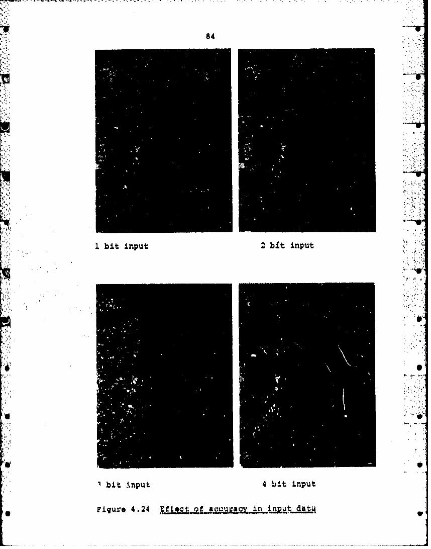
84

r:

, 11 bit input 2 bit input .

4 0"

'bit I.nput 4 bit input

Figure 4.24 Efti*t of, a(;c v~q in & datu

the receiver fcr a puJlse echo. Qv.:&ntlzation r-n amplitudebasis requires Z B sgnrn~3. ie Figure 4.24

shows an image pr.-.ýieseed ý.n 4 loo~ks with differentnumbers of bits in the irnp'it riqnal. -'he sa,-ne i'iiagewith 5 bit input is the 'a lookJ imaq~ it . Ziqlu~e 3.23.Although the quantirzatiLunVith so fow ýbi~t6 Cannot be

regarded as introducijny adtUiL~iye rioise... tý%e highcompression ratio tonfds to make th.*'aloct 0si11il.r tothe effect of additive tioiseq as cans be.-seen fro'nfigure 4.24. It can also be i~aan ttiatI the estimat4

of 3.5 bits in the intut tP ,avoi4',Vquanti~ation,'efrectg ~

is quite good. BeCause .o; additionn.1 noise introducedl.quantizati~on to for ex~ample 1, Lit x ip. i i1f y proceskiinq

4I Auof~ui for a urtlný *nR~mut I

Before t,)o aimun~h pro~qjceifg, as* bedtor u o+I~''eve t~ vstv-ma#.- c/ff .-te dopplet" t~hroiý;'And o'f ths'r'ý14tive Ve .aolty betwo~mn h, tak~gsts' wir th radarPlat."o,"'An. 1411& doppi.ev centroiv.l e t.eJ~mat~d beforethe range procwasingt %ýo only the relative vmlcc1ty V,which determines the oh.~~Gcf the az.ov, bLator~yl

* reiivins 1.1o be eatimatod.

*dhen v is known, the azimuth hist,.'j iL k w'1ifur-tion of zan~e. The ma~tched filters f:,x the 4.1.oks g':e theavs gexlerLtrid in the time domeir' hy inul~i-plyinqb~ the ~.,zimuth histor~y with the window 1unction

shown in figure 4,13, fo,: 4 ctifi,'erent, peiLtiallyoverlapping sectior~w of 'eazimuth history, eacnh1024 e.,omplex samples log The 3~inu cIed f~iteriv are

th~in the i7omplox conjugated Fourier t.ansi4orrns ofuh 100--o' timei resoansow. Theip matched filtera are

all. gene6.. ated and stored before azl.irvui~h compressiona begins.

86

One Way to estimate v is to calculate it from the orbit

parameters ol the site~lli.te. The drawback with thisprocedire Is, howevrer, that this information hastobsupplied separ-ately fromr the synthetic aperture radardata co~llection itsolf, a~nd this may take considerabletime. Dcpenaing onL ths tiLme delay,, which for SEASAT-lis on the order of days, t',his may exculude any operationaluse of the datt., T~o avt^id this difficulty "an auto-focusinc9 procedure is developed here# which means that

only the 4ata from 1-he synthatic apertur.e radar isused'Lo generate ath eitimnate of the relative velocityV.

The autofocu~sing ir based on imAximization of the contrastin thq image. Th aiiyof this criterion can beseen as follow&., -1f the azimuth compregsion is donewith an~ incorrqct va2.u6 of the relative velocity v,-wh4oh meaps wror~ ch irprat*e in the azimuth history,

th.1s will xesult in a srImaring of point targets in theimage. This sm*e4rln is equxivalent to a reduction inoc ntrmot1 It is therefore assumed that maximtum contrast.occu~rr rcr the cevireot vailue of V.

The grepter tht azimuath ban~dwidth used in the compression, .

the more sen~itive the contrast is to changes in v.Compression to 4 looks ic therefure used alio for the ,.

contrlast calculation. This has the advrAntage that therouti-ne used for azimuth com~pression of the whole image

also can L.c used here. '

The contrast C in an image is defined by (1.4), orequivalently

where I is the iritansity and <> denotes expectation.

-- - ~,, -- - - - -.... -_

The estimate for v is obtained by calculating the-,.-,:contrast curve C (v), i e contrast as a function of -••

v, for a suitable image area and choosing the value .: i

of v that corresponds to the peak in the contrast ii.i~::

curve. To get a reliable estimate for v, the area ".:,•.used for calculation of the contrast contains several

thousand image points. :i-•..

The contrast will be higher and the peak more pronouncedI, "for scen~es contairLin9 strong specular points than for

scenes with little or no strong point scatterers .....-.Scenes characterized by fully developed speckle, where .-..-. :

there are many weak specular scatterers inside a •o

single resolution cell, should not be expected toshowl any pronounced peak in the contrast curve because ,•••

the intensity, distribution in this case, given in.-,".section 3.4, does not depend on foculsing of the image. '•i'•

Figure 4.25 shows four contrast curves obtained .-:•?.experimentally from one image. The two curves in,".'",-.

S~~~the middle are from neighboring, nonoverlapping land.,.•:areas. .One of the areas is seen to have higher 1*'•

contrast than the other one, and the peak is more,,,,.•pronounced. The peaks occur, however, for the same ,'?.?.i

value of v for both areas, as was expected..,.:;•.. 1•

.. •. ~~The l~owest curve is for a homogeneous •ea area. As --.. '

• •'..: shown in section 3.4, such an area is very well -described by fully deveiloped spec~kie. According to".,..what wac said above, this should not ,,• &n area

suitable for focusing, and the contrast curve is .:':;

indeed seex. to be flat and close to the theorecical...-'value, of 0.5 for a four-look image.

.., .,

Contrast. curves for sea areas that have a pronounced. "."structure have not been calcuzlated and conclusions

a~bout f•ocusing pr"opertie.s. of suc'h areas thereforecannot be drawn.

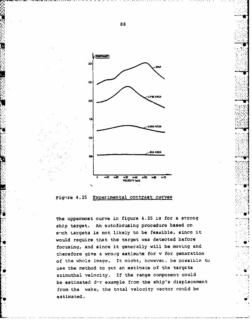
88

23.~

LI 1.,0. A FR.I

1.0I

'71.0 ;W.~ Z V 4 .w z v4-0 vo7-0VELOCITY (rn/s)

Figiire 4.25 Expeirimental contrast curves

The uppermost curve in figure 4.25 is for a strong

ship target. An autofocusing procedure based on

s"nch targets is not likely to be feaoiblet since it

4 would require that the target was detected before

*focusing, and since it generally will be moving and 7~

therefore give a wroi'g estimate for v for genaration

of the whole irnaae. It migrht, howevet, be possible tu

use the method to get an estimate of the targets

azimuthal velocity,, If the range component could ..

be estimated fr-r example from the ship's displacement

from the wake, the total velocity vector could be

estimated.

89

The ship is moving in the azimuth direction, but in

the opposite direction of the satellite, and the

peak in the contrast curve should therefore be

expected to occur for a somewhat higher velocity thanfor the land areas. The curve is, however, seen not to

have the same regular shape as for the land areaso and

the peak corresponds to a target velocity between 35 and40 knots, which is not likely to be true. Some kind ofmean value obtained from the contrast curve might givea reasonable velocity, but no good justification forsuch a procedure is seen. What can be observed..

however, is that the contrast curve is displaced inthe correct direction relative to the curves for lard

areas. This curve is also necessarily calculated for

considerably fewer image points than for the land areas,

and the statistical properties therefore cannot beexpected to be very good.

The autofocusing procedure has been tried for many

cases and has been found to work well for land areas,When imaging coastal areas, the land areas can txerefor"

be used for focusing which then also will be valid. for

athe ea s areas. aB uotiong peise m odtel forsbl th , ,. ]~,oaitasen areas by updating the orbit parameters during

passages over land.

A suitable aearch algorithm will make it necessary tocalculate only relatively few points on the contrast

cui've before the estimation procedure converges, therebyminimizing the computational burden imposed by the

autofocusing.

* 1.

90

5 TARGET DETECTZION IN IMAGES

The ultimate goal when using synthetic aperture radar inmaritime surveillance is not the images as such, but

rather a detection of targets together with an

indication of the targets' positions. When the~targets are ships,, they are approximately point targets.

The detection procedure chosen is therefore maximization

of the signal to noise ratio fcr each point. This leads

to matched filtering where the filter is matched to the

point td.rgyt responee. This is the processor developed '

earlier in this wo~rk, and the output can be interpretedas images. Target detection 4s then done in the image3

on an intensity basis.,

The method of addition ~,f diffcurpnt statistio~lly

independent looks was used to reduce the speckle inthe imaqvs. This w as done be tA~se it hasA positiv'e

aftdc t when the im ages are. regardecd '10- Lhe h'm~o,n eye,and i t also gives a better radiometric resolution,but it is not necessarily advantageous when applyingan automatic detection procedure to the images. Theaffect of look addition is considered below,.

The detection of ships in images can be done in several

ways. One method is to let a human operator perform

visual detoction in procexced images. Figures 3.14,

3.15 and 4.19-4.23 show several examples illustrating

that this is fully possible.

This detection operation should not be done fromphotographtm because of the poor dynamnic range of

intensity in photographic paper.. Use of photographs

would Alsej Incur an extra tim~e delay which for

operational purposes would be highly undeairablep.in general it can be said that a photographic

reproduction of a synthetic aperture radar image

W V M-

91

that is scaled to give a pleasant view of land areas

will, depending on sea state among other things,highly suppress strong point targets such as ships

because of the poor dynamic range in photographs.

It is seen from the examples mentioned that an interesting

way of detecting moving ships is by detection of the wake

of the ship rather than of the ship itself, or both.With a human operator this is easily achieved.

While the detection of ships in images' by means ofthe ship itself, or its wake, is easily combinedin the case of t human operator, these two methodsof tai~et detection are completely different in thecase of automatic target detection. A, method basedon detection of wakes in an image would be a patternrecognition technique, and this is not considered

here. Besides, a wake is a distributed phenomenon,

the detection of which might be done more optimally*

than by pattern recognition in an image. Anothermethod might be less time consuming than full processingof images, and this would be very important in the

case of operat.'.onal use.

As mentioned above, the detection procedure developed

here is based on the target's intensity in the image.In statistical terms this problem is called the binaryhypothesis testing problem, (17). If I is theintensity in a given image point, s is the intensitycaused by a target and n is the intensity of the sea,we have to test I against the following two hypotheses

Hit 2t=s+nH0: -n .. .

If Hi it true, the point is a combination of a tArgetand the swa, and if H0 is true, there is no target in

. . . . . . . . . . . . . . . .. . . . . . . . . ..

92

the point. Depending on the size of the target and

how much of the image point that is occupied by the

target, an alternative set of hypotheses could be .;. -

H sH0 ': I-"n .. ''Oi

In this case we have either a target or the sea in

each image point and never a combination of both. ".4

Both sets of hypotheses will be treated.

The two most used test criterions are the ones due to

Bayes and Neyman-Pearson, (17). The Bayesian

approach requires a priori probabilities of there

being a target or not and an assignment of costs

to the four different combinations of two outcomes

and true and false hypothesis. Because of the problems

in assigning reasonable values to both, the Neyman-Pearson criterion is usually applied in radar detectionproblems.

When the Neyman-Pearson test is used, only two of the

four possible combinations of outcomes and input.hypotheses are used. These are the probability of

detection, PD' which is the probability of saying that ,'6'1

H1 is true when it is true, and the probability of

false alarm, PF' which is the probability of sayingthat H1 is true when H0 is true. The criterion used -, , ."

is to maximize PD subject to the constraint P ..i e the probability of detection is maximized while

the probability of false alarm is kept below a certain .

threshold. This method thus emphasizes the importance

of not giving false alarms.

It can be shown, (17) and (1.8), that both the Bayes

criterion and the Neyman-Pearson criterion lead to a

likelihood ratio test. The likelihood ratio is

defined as

93

9(1) = ~ 1 1p (I MH

that is the ratio between the conditional probabilitiesof the cbserved intensity given H1 and H0, respectively.

The decision algorithm is then

If Z(I) > n, say H1 is true .

If 91I) . n, say H0 is true

The value of the threshold n depends on the values

chosen for P and P., The detector is thus aprocessor that generates the likelihood ratio Z (1)

for each image point and decides which hypothesisis true by comparing (I) with the .threshold n. .

To find the performance of the detector it is necessaryto calculate the likelihood ratio I(I) and th•e socalled "*"!

receiver operating characteristics, curves of P verIsusP., for the dif ferent cases We thus need the

probability distributions for the intensity subject

to the two hypotheses, and for different cases suchas different numbers of looks.

The probability distribution for the intensity in a

onelook image of a son area is supposed to be givenby the probability distribution for fully developed

speckle. This distribution was given in 3ection 3.4,

and if it is normalized by satting Io - i, we got

PI(II,) - exp{-I), 1>0 and zero elsewhere.

The subscript indicates the number of looks. The

addition of several looks is equivalent to the .

addition of several independort, identically distri-

buted stochastic variables. The resulting probability

distribution i.s then the convolution of the individualdistributions• Thbir 13 mos,' ;3sily accoriplished

PC. V T- ... .. -

94

mathematically by applying the moment generating

function which is defined by

M(S) = f p(x)'exp{-sx}dx

where p(x) is the probability distribution. The

moment generating function for a sum of independentstochastic variables is the product of the individualmoment generating functions. Sinoe we here always

have p(x) - 0, x < 0, the moment genrating function

is equal to +,he onesided Laplace transform of p (x).

We thus get

o,= r pi XIH 0 )•Zp{-s!}d! ! exp{-(s+l)I}dI - (2+l)'".0 0

The moment generating funt•ior, for n looks is

invc.rs,i Laplace traasformaticj., gives .....

.n-1.

where r (n) is the Vanmna fnction.

Since we have H 4o, we aluo have pz.(I H P (11 )

To find pn,(IIHL) and pn(I it.I') we must know the

probabilikq ditri;-tic., of iu, i. the ta;9,t'"

intensity distrbution. Dqaause of the inherent

diffidulties in defining this distribution, the n,oe.

reasonable 9robabll"ty distribut.o o is assurped tobsi a anifornm 1,stributio'%. We chus have

95

ps =( O<s<S

0

The significance of the choice of S will be commented0

upon later.

When adding looks, the targets' intensitites and the

"intensity of the sea background will be statistically

independent, and the distribution p(IIHI = p(Ils+n)is the convolution of the probability distributions

for target intensity and sea intensity. When processing

images it has turned out, however, that there is strong

interdependence between different looks for strong

targets. This is not unexpected since a strong targetmay consist of perhaps only a single strong reflectingpoint. The intensity distribution for a target after

look addition is therefore not obtained by convolution

of the single look distribution with itself several

times, but is better modelled by a uniform distribution

even after look addition, properly scaled according

to the new mean value.

By scaling all the speckle distribution functions to

have mean values equal to 1, we get the following

distributions.

n-Pn(IIH') pnoo' 0-- sexp{-n, I > 0

The distribution Pn(IIHI) is given by the convolutionof Pn(IIH0) and Pn(IIHl')

Pn(IIH:) f ! .(xIHO )dx r(n) f0 ( I xn0 "exp-nxdx

-El-exp{-nI} I r-)m O< I < S V0 m=o

rJ -. -. o' .--.

96-.

The tail of the distribution Pn(IIHl) for I>So is not

calculated since it is not needed.

The likelihood ratios can now be calculated

in () n(IIHo S0*nnn-in) (n1 (ni) m ....'Pn(IHI)= rn--).I-n-l[exp{nI}- T - . "..•!:

so.n m=o

0-< I. < S- -0

PnlIIHI'), , =rnL.I-(n-l)-exp{nI}, 0 < I < So!p (1 H IT' n 0-:..•..£n Pn( 0~ soon , ..

Since .

exp~n~l(nI)mexp{nI}-' E .,,m-0

we have

n(i) r(n) .- (n-l) mn (nI)m r(n). Z (nI)m-n+lSo~inn M! m =soonmn m'-•••:.Ssoon o r-n n

We therefore have dL[Xn(I)]>0 for 0<I<S while for'd dI n 0 I d"

S'(I) we have TI[in' (I)]< for 0<I<l and I[n'(I)]>o

for I•<I<So. Also kn' (I)40k when 1*0. This means

that Zn' (I) cannot be used for the interval 0<1<l-."nnThe detector will therefore operate as follows for

the different intensity intervals.

Hypotheses H0 and H1:

0<I<So: H true if Z (I)<n

H1 true if Z (I)>nIo n

1>S :H true0 1

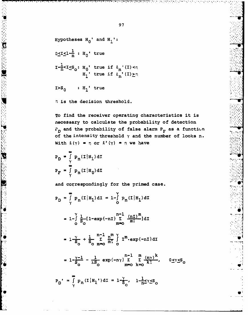
97

Hypotheses H 'and H0

O<I<l-.jj H 0 true

n 0

H1 true if z~ '(I) >nn

i>S0 H1 true

nl i s the decision threshold.

To find the receiver operating characteristics it is

necessary to calculate the probability of detection

Padthe probability of false alarm P Fas a functiGn

of the intensity threshold y and the number of looks n.

KWith Y,(Y) -nor X,'(y) n r we have

P fp (IIHI~dI

and correspondingly for the primed case.

- Y

D f Pn(I IHj.)dI 1 -f Pn(I 1 dY 0

-l(nI)md=1-f g-[l-exp{-nI) I B-d

0 0 Min0

1 -~+~ En-lnmf I exp{-.nI}dI

n-l m (k

(n--o

98

= P f Pn(IIHo)dI = n f In exp{-nIldIY Y

.nn - (n-l) k= •~~ .exp{_nY}n 1 Z.,,..k-an

:-i = exp{-ny} £ , kk=o n.~ >

The probability of detection PD is seen to depend

strongly upon SO, which means that a somewhat

arbitrary choice of SO will have considerable

effect upon the resulting probability of detection.

Since one can write

=D l- -. f (y,n) ,•...-'

where f(y,n) is a function of y and n, the dependence

of PD upon n, the number of looks, can be found by

studying f(yn) which does not depend on So.

The reason why the number of looks n is an importan...

parameter with regard to target detection is the

relationship between the coherence time of a target and

the coherent integration time in the processor. By -

coherence time of a target is meant the longest

observation time during which the target response

can be regarded as coherent. The peak response for

a target will increase more strongly for an increase

in coherent integration time when this integration

time is shorter than the target's coherence time than

when it is longer. The coherence time of the sea

background, regarded as speckle noise, is of no importance .

in this case since the speckle distribution functions are

independent of coherence time. Since the length of the

synthetic aperture is fixed, there is a compromise between

coherent integration time (integration time per look) and W'

number of looks.

-~ ---.- v .-- - - - - - - - - j I

99

When comparing the receiver operating characteristics

for different numbers of looks, this must be done with

the same amount of input information in each case to

get relevant results. This means that the total inte-

gration time used for a given number of looks must be

the same for all cases compared. This total integration

time, given by the length of the whole synthetic aperture,

is assumed constant for all cases considered.

The formulas developed above are all derived by means

of speckle distributions which have an expected value

of 1. This represents an intensity scaling. S0 is also

the same in all the formulas.

As a parameter in the comparison Of different cases a

coherence factor kc will be introduced. This factor is

defined below.

If the case of a single look, i e n 1 1, is described

by an expected speckle intensity of 1 and a target

intensity distribution that is uniform on the interval

0<<_SO, the case of n looks can be described by an

expected speckle intensity of 1 and a target intensity

distribution that is uniform on the interval O<I<k S

We will always have <k. •l, where a high value of

target coherence time relative to the coherent integration

time in the processor corresponds to a low value of kc.

This can be seen as follows.

Given an image which contains n looks. If the coherent

integration time is increased to the case of one look,the peak intensity of the target relative to the sea in the -..-.

onelook image will change from the case of n looks .- '

depending on the coherence properties of the target.

As mentioned above the speckle distribution is independent

of sea coherence time, and the mean value of the speckle

intensity is proportional to the bandwidth of the chirp-filter when the input speckle noise is considered white

100

in the frequency band of interest. Mean speckleintensity is therefore proportional to coherent inte-

gration time. If the target is coherent over the

whole observation time, an increase in coherent inte-

gration time with a factor n will result in a peak2

intensity increase for the target with a factor n ,Since the mean sea intensity increases with a factor

n, this gives kc = The other extreme case is when• nthe target coherence time is shorter than the coherent

integration time corresponding to n looks. In this case

target peak intensity increases incohezently, i eproportionally with coherent integration time, and we

have kc 1.

Figures 5.1 and 5.2 show the receiver operatingcharacteristics for kc = 1, kc - 1 and n = 1,2,3,4.

Sc0 is chosen 100. Only the primed case is shown sincethe unprimed case exhibits the same principal behaviour.

The figures show that in the case of kc - 1, the

maximum number of Locoks should be chosen, and when

kc = I, one look should be chosen. This is intuitively

logical since in the first case there is nothing to be

gained by increasing the coherent integration time, while

averaging of several looks will suppress the upper tail

of the sea intensity distribution, thereby increasing the

detection probability for a given false alarm probability.

Likewise for kc = i, the target detection probability is 2highest when using a single look.

Since the order of the receiver operating characteristicsin figures 5.1 and 5.2 for different values of n is seento be reversed, there is obviously a value of kc for

which the receiver operating characteristics for two

given numbers of looks are equal for any chosen value

of false alarm probability PF"

*10

30

2 OKS• .:>••

0.LO0

I UM

2LO0 ID P-"-•

Figure 5.1 Receiver operating characteristics withk ~1

0•-C-

To be able to choose the optimum number of looks, the

coherence properties of typical targets must be known.

These properties can be expressed by a function that

shows how the expected peak intensity of a target changeswith coherent integration time, that is integration time

per look

If T is the total integration time, i e the length of

the azimuth history, then g(T) = • gives the normalized

expected intensity of the sea, where T is the coherentintegration time, O<_<T. f(r) is the corresponding curvefor a target, and it is closely related to the correlationfunction of the target's azimuth history. f(T) can best

be obtained empirically. Figure 5.3 shows g(T) and apossible normalized f(T).

• . . -

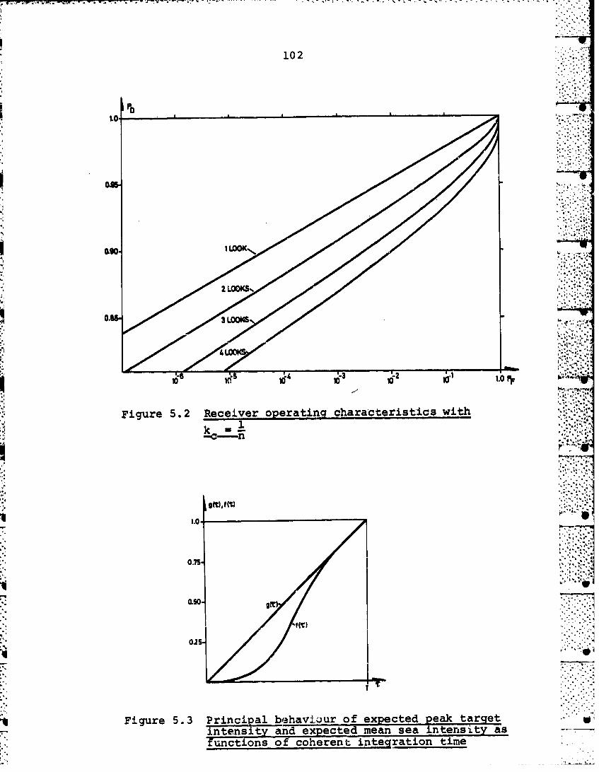
102

1.0

0II

0.00

-. 6~~~ 4413 -

Figure 5.2 Receiver operating characteristics with

k

-C-flMLo4 .'p4

T.ii1 .0f ( 1 ).

Figure~~~ ~ ~ ~ ~ ~ 5.3 Prnialbhvou fepetd2ktre

intesityand xpeced man sa inensiy a

0.7 cton of coeetitgaintm

103

The parabolic portion of f(T) gives the integration

times f or which the target response is highly coherent.

The linear portion of'f(T) represents an incoherent

increase in peak intensity as the coherent integration

time is increased.

To find the optimum number of looks the receiver

operating characteristics must be plotted. The curves .:o .. ,

g(T) and f(T) will then determine the coherence factor

ko, which is given as a function of n by the expressionc

n nk0 (n) n () -nf(j)

,'S- 4'. " ,

if the functional form of f(T) were known, the optimum

number of looks could be calculated. Instead a single3,,. case with a ship target has been tried experimentally '.

by processing to 1 and 3 looks, respectively. By

comparing the peak intensity of the ship with the mean

intensity of the surrounding sea, a coherence factor of

0.59 was found. Figure 5.4 shows the receiver operatingcharacteristics for 1 and 3 looks with k - 0.59. It is

c"seen from the figure that in this case it is advantageous,.

to use 3 looks if a false alarm rate less than approxi-

mately 5•10- is desired.,-~...

A generalization not considered here is to use over-

l•.pping looks. This would give partially correlatedlooks and the resulting receiver operating characteri-

stics would be somewhat different from the ones derivedabove.

Since the total integration time is constant, the

azimuth resolution will be degraded as the number

"of looks is increased. Depending on the target size,

.''_________________________

104

000

Piur 5.4 'Receiver oprtn 'characteristics fo'an experimenta.l case

this may lead to a isuppression of the target if it

becomes much smaller than the resolution cell. For a

SAR system like the one onboard SEASAT-l it seems

uinlikely that it should be advantageous to use so many

looks that this might occur.

105

S '"4, 544w J,°

6 CONCLUSION

As has been shown in the previous chapters, a satellite -- : .

borne synthetic aperture radar can very well be usedfor maritime surveillance purposes. It is seen from

the examples of processed imagery that in many casesships can be seen clearly against the sea background.An especially interesting phenomenon is the clear

visibility of the ship's wake, which probably appearsmore clearly and lasts longer than it would in imagesobtained in the optical frequency band.

The autofocusing procedure developed has been tried for

many different cases and works well for land areas.

Such a method is necessary when operational use of the

SAR imagery is intended, and may, depending upon the '4""

quality of the estimation algorithms used for thesatellite orbit parameters, be adequate for maintainingcorrect focus setting also for sea areas by updating

the estimates during passes over land.

When using the SEASAT-1 SAR system to evaluate theusefulness of a satellite borne SAR system for mari- -..,

time surveillance, it should be remembered that this

system was not designed for such a purpose. Some of

the design criteria were in fact the opposite of what "'would be chosen for surveillance purposes. The

depression angle of 70° was for example, among otherreasons, chosen becausze this gives a rather high ..-.4

backscatter coeffisient for the sea. When looking

for ships this results in a high sea clutter level

which makes the target detection more difficult. A

somewhat smaller depression angle would result in a

lower sea clutter level.

The main problem when using a satellite borne -AR

system for maritime surveillance, and digital proces-

sing of images, is the procesaing time. To be of any

________•__

106

operational value, the images would have to beprocessed within a few hours after the satellite

had passed the area. The average processing ratewould also have to be equal to the data acquisition

rate. If the data rate is measured in kmh/sec, the

acquisition rate for SEASAT-I was approximately700 km /sec. The images shown here are processed

with a general purpose computer and with a rate of

approximately 60 km2 /hour 0.017 km2 /sec. If the .average acquisition rate for an operational systemshould be of the order of 10 km 2/sec, this would

require an increase in processing speed with a factor600.

The target detection ,algorithm developed in chapter 5 ,

will require processing to obtain empirical values forcoherence times for typical targets. This has notyet been done, but a single example is given whichillustrates the effect of changing the coherentintegration time.

. ',

4''

-:2--.

"C2:°.

APPENDIX A 107

DOPPLER CENTROID ESTIMATION

The doppler centr.•id of the azimuth frequency spectrumis estimated dirsctly from a block of rawdata. The

real samples are converted to complex samples bydemodulating the range vectors so that the lowest

"k sideband is centered around 0 frequency, and thenlowpass filtering each range vector to reduce the3ampling frequency with a factor 2. Each azimuth

vector is then Fourier -transformed, the spectrum isaveraged over 100 azimuth vectors, each of length 512complex samples, and the doppler centroid is estimatedfrom the phase of the first harmonic of the frequency

spectrum.

Rawdata block with real samples

a(i,j), i = 0,208, j = 0,511, <a(i,j)> 0

i is range index and j is azimuth index. The lowest

sideband in range is centered at 11.38 MHz, which is

the real sampling frequency divided by four. Demodu-

lation gives "

b(ij) = a(i,j).exp{-j7.i}, i = 0,208, j = 0,511

Lowpass filtering with a truncated interpolationfilter gives the rawdata matrix on complex form

10 sin[ (k-5)-]2c(i,j) = Z b(2i+kj).--- , i = 0,99, j = 0,511

k=o (k-5)-

Fourier transformation in azimuth

.6 ~511Hi(k) Z c(i,j)-exp{-j 2-gk.j}, k = 0,511, 1 = 0,99

j=o

108

Averaged frequency spectrum

W (k) -F Z IsJ1(k) I k =0,511

First harmonic of WG W is

511d -W~k .ex{-j~1 =rd -exP{-i~dl, cl2

k-o

The doppler centroid estimate fd is then

A

PEP is the pulse repetition frequency of the radar.

Through use of this estimation algorithm it seems

that an accuracy of better than 100 Hz is obtained T

with PEP -1647 Hz.

109

References

(1) Skolnik M I (1962): "Introduction to radarsystems", McGraw-Hill, Inc.

(2) Tomiyasu K (1978): "Tutorial review ofsynthetic-aperture radar (SAR) with applicationsto imaging of the ocean surface", Proceedingsof the IEEE, Vol 66.

(3) Brown W M, Porcello L J (1969): "An introductionto synthetic aperture radar", IEEE Spectrum, No 9.

(4) Jordan R L (1980): "The SEASAT-A syntheticaperture radar system", IEEE Journal of OceanicEngineering, Vol OE-5, No 2.

(5) Thomas J B (1969): "An introduction to statisticalcommunication theory", John Wiley and Sons, Inc.

(6) Rondinelli L A, Zeoli G W (1962): "Evaluation ofthe effect of random tropospheric propagationphase errors on synthetic array performance",Eighth Annual Radar Symposium Record, Universityof Michigan.

(7) Greene C A, Moller R 'T (1962): "The effect ofnormally distributed random phase errors onsynthetic array gain patterns", IRE Transactions

'Uilitary Electronics, Vol MIL-6, No 2.

(8) Goodman J W (1968): "Introduction to Fourieroptics", McGraw-Hill.

(9) Goodman J W (1976): "Some fundamental propertiesof speckle", Journal of Optical Society ofAmerica, Vol 66, No 11.

(10) Cutrona L J, Leith E N, Porcello L J, Vivian W E(1966): "On the application of coherent opticalprocessing techniques to synthetic aperture radar",Proceedings of the IEEE, Vol 54, No 8.

(11) Leith E N (1968): "Optical processing techniquesfor simultaneous pulse compression and beamsharpening", IEEE Transactions on Aerospace andElectronic Systems, Vol AES-4, No 6.

(12) Harger R 0 (1970): "Synthetic Aperture RadarSystems", Academic Press, Inc.

(13) Eklundh J 0 (1972): "A fast computer method formatrix transposing", IEEE Trans C-21.

110

(14) Rabiner L R. Gold a (1975): "Theory andapplication of digital signal processing",Prentice-Hall, Inc.

(15) Brigham E 0 (1974): "The Fast Fourier Transform",Prentice-Hall, Inc.

(16) Herland E A: Report in preparation.

r(17) van Trees H L (1968): "Detection, Estimation andModulation Theory",, Part 1I, John Wiley & Sons, Inc.......

K(18) Wainstein L A, Zubakov V D (1962): "Extractionof signals from noise", .Prentice-Hall.

.4.7.