Embed Size (px)
Citation preview
© 2005 Ingenuity Systems Proprietary and Confidential 1
IPA Network Generation Algorithm
October 29, 2005
Section 1. Purpose Ingenuity Pathway Analysis (IPA) is a system that transforms a list of genes (with or without accompanying expression information) into a set of relevant networks based on extensive records maintained in the Ingenuity Pathways Knowledge Base (IPKB) [1, 2]. This knowledge base has been abstracted into a large network, called the Global Molecular Network, composed of thousands of genes and gene products that interact with each other. For simplicity in this document we will use the term gene to describe both genes and gene products. A relationship between two genes in this network is called an “edge”. Two genes are connected if there is a path in the network between them, i.e., a series of genes and edges that connect one gene to another. Most genes in the Global Molecular Network are connected to each other, i.e.: if we start at any random gene we will find it is most likely eventually connected to most other genes. How, out of this extremely large Global Molecular Network, can we choose a small number of genes to display as a relevant interaction network? There are three basic principles behind the design of the network generation algorithm used in IPA. These principles, which are based on interviews with scientists about what characteristics would most useful in networks generated from their expression datasets, are as follows:
1. We want to return networks that help biologists understand how their genes of interest are biologically related, preferably by showing as many interactions between user-specified genes as possible so as to be most informative about how the genes in a given dataset appear to work together at the molecular level. In cases where we cannot directly connect the genes, we relate them via other neighboring genes in the Global Molecular Network.
2. We believe that highly-interconnected networks are likely to represent significant biological function [3-6] (see Appendix), so we optimize for “triangular” relationships between genes, in essence favoring denser networks over more sparsely-connected ones. Note that while we believe this to be a good starting point for analysis, it is by no means the only approach. There are other approaches to identifying interesting biological functions that are supported through IPA’s interactive features (e.g. directly querying for genes involved in particular biological processes, or using the “Grow Out” functionality to search for sparsely-connected chains of interactions that may represent signaling events).
3. We want to give users a maximally useful amount of information on a single screen while still producing interpretable networks, so we aim to build networks that are initially about 35 genes in size. Subsequent operations can then expand
upon these starting networks by merging them, growing them to larger sizes, etc.
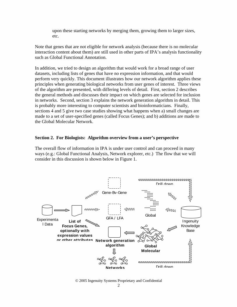
Note that genes that are not eligible for network analysis (because there is no molecular interaction content about them) are still used in other parts of IPA’s analysis functionality such as Global Functional Annotation. In addition, we tried to design an algorithm that would work for a broad range of user datasets, including lists of genes that have no expression information, and that would perform very quickly. This document illustrates how our network algorithm applies these principles when generating biological networks from user genes of interest. Three views of the algorithm are presented, with differing levels of detail. First, section 2 describes the general methods and discusses their impact on which genes are selected for inclusion in networks. Second, section 3 explains the network generation algorithm in detail. This is probably more interesting to computer scientists and bioinformaticians. Finally, sections 4 and 5 give two case studies showing what happens when a) small changes are made to a set of user-specified genes (called Focus Genes); and b) additions are made to the Global Molecular Network. Section 2. For Biologists: Algorithm overview from a user’s perspective The overall flow of information in IPA is under user control and can proceed in many ways (e.g.: Global Functional Analysis, Network explorer, etc.) The flow that we will consider in this discussion is shown below in Figure 1.
© 2005 Ingenuity Systems Proprietary and Confidential 2
Experimental Data
List of Focus Genes,
optionally with expression values or other attributes Network generation
algorithm
Networks
Global Molecular
Ingenuity Knowledge
Base
Gene-By-Gene
GFA / LFAGlobal
Drill down
Drill down
© 2005 Ingenuity Systems Proprietary and Confidential 3
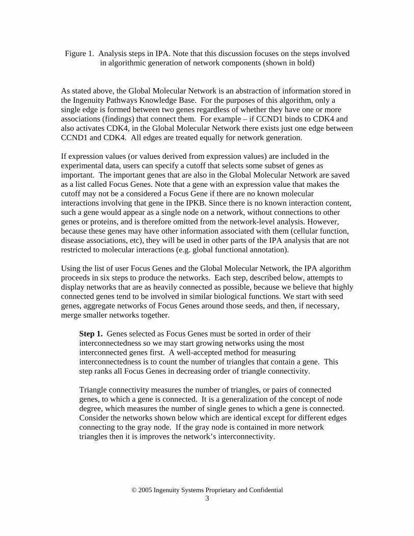
Figure 1. Analysis steps in IPA. Note that this discussion focuses on the steps involved in algorithmic generation of network components (shown in bold)
As stated above, the Global Molecular Network is an abstraction of information stored in the Ingenuity Pathways Knowledge Base. For the purposes of this algorithm, only a single edge is formed between two genes regardless of whether they have one or more associations (findings) that connect them. For example – if CCND1 binds to CDK4 and also activates CDK4, in the Global Molecular Network there exists just one edge between CCND1 and CDK4. All edges are treated equally for network generation. If expression values (or values derived from expression values) are included in the experimental data, users can specify a cutoff that selects some subset of genes as important. The important genes that are also in the Global Molecular Network are saved as a list called Focus Genes. Note that a gene with an expression value that makes the cutoff may not be a considered a Focus Gene if there are no known molecular interactions involving that gene in the IPKB. Since there is no known interaction content, such a gene would appear as a single node on a network, without connections to other genes or proteins, and is therefore omitted fr the network-level analysis. However, bdisease asso at are not
stricted to molecular interactions (e.g. global functional annotation).
o ly
network triangles then it is improves the network’s interconnectivity.
omecause these genes may have other information associated with them (cellular function,
ciations, etc), they will be used in other parts of the IPA analysis thre Using the list of user Focus Genes and the Global Molecular Network, the IPA algorithm proceeds in six steps to produce the networks. Each step, described below, attempts tdisplay networks that are as heavily connected as possible, because we believe that highconnected genes tend to be involved in similar biological functions. We start with seed genes, aggregate networks of Focus Genes around those seeds, and then, if necessary, merge smaller networks together.
Step 1. Genes selected as Focus Genes must be sorted in order of their interconnectedness so we may start growing networks using the most interconnected genes first. A well-accepted method for measuring interconnectedness is to count the number of triangles that contain a gene. This step ranks all Focus Genes in decreasing order of triangle connectivity. Triangle connectivity measures the number of triangles, or pairs of connected genes, to which a gene is connected. It is a generalization of the concept of nodedegree, which measures the number of single genes to which a gene is connected. Consider the networks shown below which are identical except for different edges connecting to the gray node. If the gray node is contained in more
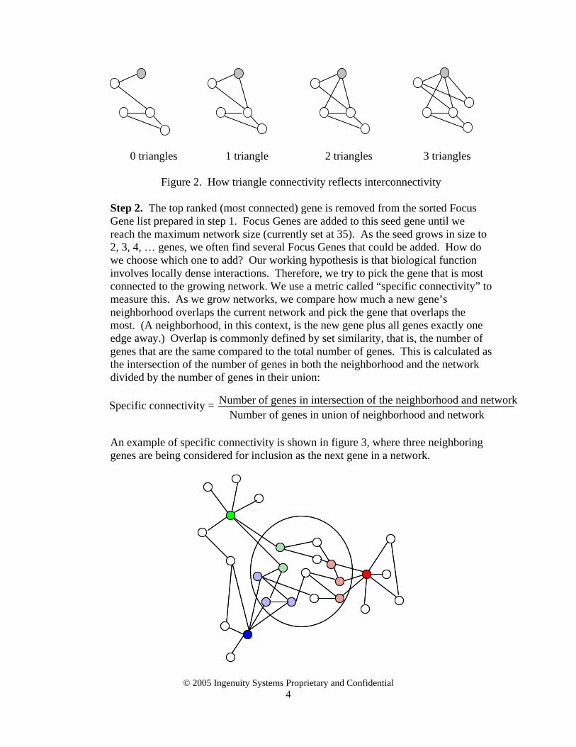
0 triangles 1 triangle 2 triangles 3 triangles
Figure 2. How triangle connectivity reflects interconnectivity
w do
iological function volves locally dense interactions. Therefore, we try to pick the gene that is most
connected to the growing network. We use a metric called “specific connectivity” to measure this. As we grow networks, we compare how much a new gene’s neighborhood overlaps the current network and pick the gene that overlaps the most. (A neighborhood, in this context, is the new gene plus all genes exactly one edge away.) Overlap is commonly defined by set similarity, that is, the number of
enes that are the same compared to the total number of genes. This is calculated as
ivided by the number of genes in their union:
Step 2. The top ranked (most connected) gene is removed from the sorted Focus Gene list prepared in step 1. Focus Genes are added to this seed gene until we reach the maximum network size (currently set at 35). As the seed grows in size to2, 3, 4, … genes, we often find several Focus Genes that could be added. Howe choose which one to add? Our working hypothesis is that bin
gthe intersection of the number of genes in both the neighborhood and the networkd
© 2005 Ingenuity Systems Proprietary and Confidential 4
An example of specific connectivity is shown in figure 3, where three neighboring genes are being considered for inclusion as the next gene in a network.
Number of genes in union of neighborhood and network Number of genes in intersection of the neighborhood and network Specific connectivity =
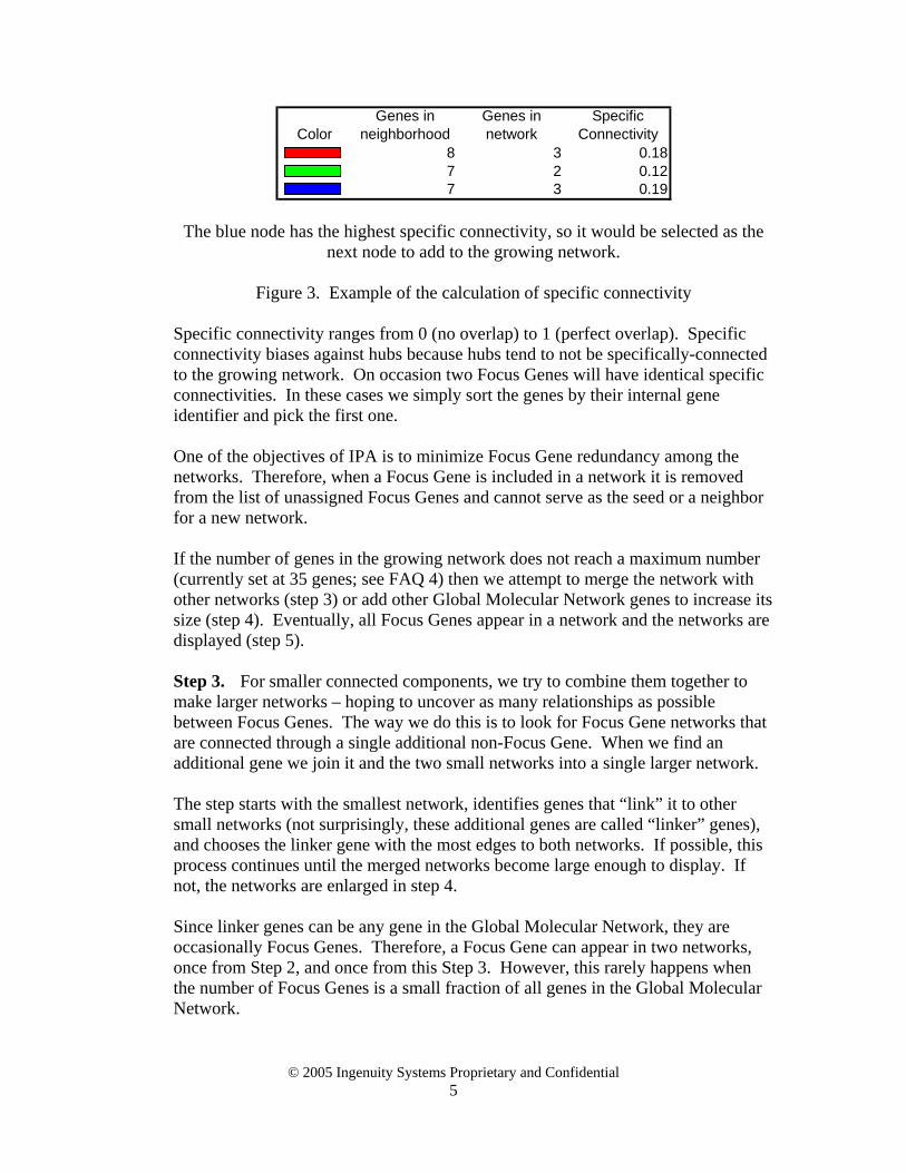
ColorGenes in
neighborhoodGenes in network
Specific Connectivity
8 3 0.187 2 0.127 3 0.19
The blue node has the highest specific connectivity, so it would be selected as the
next node to add to the growing network.
Figure 3. Example of the calculation of specific connectivity Specific connectivity ranges from 0 (no overlap) to 1 (perfect overlap). Specific connectivity biases against hubs because hubs tend to not be specifically-connected to the growing network. On occasion two Focus Genes will have identical specific connectivities. In these cases we simply sort the genes by their internal gene identifier and pick the first one. One of the objectives of IPA is to minimize Focus Gene redundancy among the networks. Therefore, when a Focus Gene is included in a network it is removed from the list of unassigned Focus Genes and cannot serve as the seed or a neighbor for a new network. I(ther networks (step genes to increase its ze (step 4 works are isplayed (
two small networks into a single larger network.
il the merged networks become large enough to display. If
s Genes is a small fraction of all genes in the Global Molecular
f the number of genes in the growing network does not reach a maximum number currently set at 35 genes; see FAQ 4) then we attempt to merge the network with
3) or add other Global Molecular Network osi ). Eventually, all Focus Genes appear in a network and the net
step 5). d Step 3. For smaller connected components, we try to combine them together to make larger networks – hoping to uncover as many relationships as possible between Focus Genes. The way we do this is to look for Focus Gene networks that are connected through a single additional non-Focus Gene. When we find an dditional gene we join it and thea
The step starts with the smallest network, identifies genes that “link” it to other small networks (not surprisingly, these additional genes are called “linker” genes), and chooses the linker gene with the most edges to both networks. If possible, this rocess continues untp
not, the networks are enlarged in step 4. Since linker genes can be any gene in the Global Molecular Network, they are occasionally Focus Genes. Therefore, a Focus Gene can appear in two networks, once from Step 2, and once from this Step 3. However, this rarely happens when he number of Focut
Network.
© 2005 Ingenuity Systems Proprietary and Confidential 5

© 2005 Ingenuity Systems Proprietary and Confidential 6
e
em to any gene in the network. If there are no genes with two or more edges then es
, the added genes can be Focus Genes but rdinarily the probability is low.
e r,
Genes, small networks are the only ones that appear in the Global olecular Network. In this case we report the small networks because we want to
alculated using Fisher’s exact test as described in ction 3, step 6. Since interesting p-values are typically quite low (e.g.: 10-8) it is
Step 4. For those networks that still have less than 35 genes, other genes are added to the periphery of the network to provide additional biological context to thosfocus genes. We start by adding genes that have two or more edges connecting thwe add new genes with only a single edge to some gene in the network. Sometimseveral genes have the same number of edges to the network and we have to chooseamong them. If the data set has expression data, we can break the ties by choosing genes with the greatest expression values. Otherwise, we select them by order of their internal gene identifier. As in step 3o Step 5. Network genes and all edges between them are pulled together into a singlnetwork. We intend that these networks contain approximately 35 genes. Howeveoccasionally we find that, despite our attempts to merge and grow networks with non-FocusMshow each Focus Gene in at least one network. Our assumption is that even if a Focus Gene is only connected to one other gene in the GMN, this network is of value and should be displayed. Such small networks have low p-scores and are displayed toward the end of the results. Step 6. The final step is the calculation of p-scores used to rank networks on the IPA “Results” page. The p-scores are derived from p-values. Say there are n genesin the network and f of them are Focus Genes. The p-value is the probability of finding f or more Focus Genes in a set of n genes randomly selected from the Global Molecular Network. It is csevisually easier to concentrate on the exponent. Therefore, the p-score is defined as: value)-(p log- score-p 10=
© 2005 Ingenuity Systems Proprietary and Confidential 7
Frequently Asked Questions (FAQs) about the network generation algorithm FAQ 1. What types of relationships from the knowledge base are used to build networks? The Global Molecular Network contains both direct and indirect relationships. For example, the finding that “CREB increases expression of Cyclin D1” is considered a direct relationship between the transcription factor CREB and the gene Cyclin D1. In contrast, the finding that “IFNg increases expression of Cyclin D1” is considered and indirect relationship, as IFNg is not able to directly bind to and increase the transcription of the Cyclin D1 gene. Both types of interactions can provide useful information about gene interactions, and in IPA users can choose one or both. FAQ 2. Does the algorithm utilize the expression values associated with my Focus Genes? Focus Genes may be specified by users directly (using the override feature) or identified by IPA via a user-defined cutoff for expression values associated with each gene. Once Focus Genes are selected, the magnitude of an expression value is used only in Step 4 for breaking ties among non-Focus Genes. In general, the user-provided expression values are not used to infer network connectivity beyond the selection of focus genes. This enables the same algorithm to work equally well on arbitrary lists of user genes that may not have associated expression levels, fold-changes, or other quantitative ranks. FAQ 3. Why are networks limited to 35 genes? The largest network generated contains 35 genes. We experimented internally with different network sizes and found we had to accommodate several constraints: a) the network diagram had to be small enough to include useful information on a computer screen; b) the network had to be large enough to show interesting biological interactions; and c) the network had to be small enough to allow analysis calculations to run quickly (minutes rather than hours). Our balance of these constraints was to limit networks to 35 genes and to allow users to interactively create larger networks by merging several smaller ones (up to 210 genes). FAQ 4. Why do I get high-scoring networks when I submit a random list of genes? The purpose of IPA’s network generation algorithm is to find networks of highly connected Focus Genes. If users submit Focus Genes chosen at random, IPA will still do its best to bring as many of these Focus Genes into a single network as possible. Since most genes can be connected through one or more intermediate genes in the GMN, IPA can often connect even random lists of genes to produce networks. Note that once the
© 2005 Ingenuity Systems Proprietary and Confidential 8
networks are constructed they are scored using only the Focus Genes and not the connectivity of the network itself. Thus, because many Focus Genes can appear in a network, and the score is simply a measure of the number of Focus Genes in a network, networks of random can often receive a high score. FAQ 5. What is the relationship between biological function and network interactions? Optimizing networks with respect to the number of internal edges is based on the observation that biological function involves locally dense interactions between genes[3-6]. In order to verify that biological function is in fact related to dense subnetworks of our Global Molecular Network we have performed a quantitative statistical analysis using known functional annotations of genes[3], which is summarized in appendix 2. Section 3. Detailed description of algorithm The IPA network generation algorithm has five core design goals:
1) Analyze user-specified lists of genes, some of which may have expression values or ranks associated with them (but the algorithm must work with simple lists of genes as well);
2) Highlight the molecular biology implied in a dataset by identifying how user-specified genes interact with each other or with neighboring genes;
3) Prefer highly-interconnected molecular networks over sparsely connected ones because the former tend to reflect significant biology ;
4) Generate non-redundant networks that are manageable in size and can be easily visualized and understood.
5) Analyze datasets quickly, i.e., perform computations quickly enough that a typical dataset can be analyzed while a user is waiting
The selection of high scoring networks, typically based on gene expression data, has been well studied in the literature, and several authors have solved one or more of the above goals, often using objective functions. Ideker looked for subnetworks in protein-protein and protein-DNA networks that maximized an overall subnetwork function based on expression data [7]. Rajagopalan integrated three distinct networks and improved on Ideker’s optimization function [8]. Pradines combined metabolic and regulatory pathways from two databases to compute the inverse problem: what genes have significantly upregulated neighborhoods, where neighborhoods are defined using the networks [9]. Bader addresses gene network interconnectivity using a pre-existing interaction network [10]. Unlike these algorithms, Ingenuity constructs networks that optimize for both interconnectivity and number of Focus Genes under the constraint of a maximal network size.

© 2005 Ingenuity Systems Proprietary and Confidential 9
Ingenuity’s approach is based on a multi-stage, heuristic algorithm that executes six steps to try to satisfy all of the above goals. The IPA network generation algorithm iteratively constructs networks that greedily optimize for both interconnectivity and number of focus genes under the constraint of a maximal network size. The six steps are:
1. Sort focus genes with respect to their interconnectivity. Highly interconnected focus genes will be processed first. Optimizes triangle connectivity.
2. Construct networks from Focus Genes. Optimizes number of Focus Genes and number of specific edges (measured using specific connectivity) within each network.
3. Merge small networks using linker genes. Optimizes edge connectivity. 4. Grow small networks using neighborhood genes. Optimizes edge connectivity. 5. Form all edges between genes. 6. Compute the p-score.
It is occasionally the case that, during an optimization, several genes will score equally. In such cases, IPA chooses genes by sorting them in the order of an internal identifier and choosing the first one. Each step is described below following a summary of the algorithm definitions.

Definitions:
a) Let F be the set of user genesU that the user considers to be interesting (e.g. all genes that are above a certain expression value or below a p-value cut off).
b) Let the graph ),( EVG = represent the Global Molecular Network, where V is the set of nodes representing genes and E is the set of edges representing interactions. G contains no self edges.
c) Let be the set of focus genes, i.e. the set of genes
inVFFG ∩=
F that are also contained in the Global Molecular Network.
d) Let denote the neighborhood of a node v inG . is the set of all nodes adjacent to
)(vNG
VvNG ⊂)( Vv∈ . Similarly let denote the neighborhood of a set of nodes inG .
)(SNG VS ⊂
e) Define the triangle connectivity ) of a node (vtrG Vv∈ as the
number of triangles inG that contain v .
f) Define the specific connectivity of a node Vv∈ with respect
to a set of nodes as VS ⊂|]}{ )([|| }]{ )([|),(
SvvNSvvNSvsc
G
GG ∪∪
∩∪= .
g) Define the edge connectivity of a node Vv∈ with respect to
a set of nodes as VS ⊂ SvNSvec GG ∩= )(),( .
h) Define the user-score ) of a node v(vusG V∈ as the average of the user-provided scores of UvvNG ∩∪ }]{ )([ . Scores such as expression values, p-values, etc., are part of the user’s input dataset. Scores are changed so the most significant scores have larger values.
i) Define two sets of node sets in , the display list and the
candidate list C . G D
j) Let be the maximum number of nodes in displayed networks. In the actual implementation of the algorithm we set .
maxN
35max =N
© 2005 Ingenuity Systems Proprietary and Confidential 10

Step 1: Sort Focus Genes by triangle connectivity 1.1. Initialize andC to be empty sets, D ∅=D , ∅=C .
1.2. Initialize to be the set of unused focus genes. GG FF =' 1.3. Pick the node with the largest triangle connectivity
in . Update
'GFv∈
)(vtrG'
GF { }vFF GG \'' = and initialize a set of nodes . { }vS =
Step 2: Greedily construct networks of Focus Genes up to a
maximum pre-defined size.
2.1. Make a set of all neighboring focus genes of . Pick the node
')( GG FSNN ∩=S Nw∈ with the largest specific
connectivity sc with respect to . Update .
),( Sw
G
NS
S{ }wSS ∪=
2.2. Repeat step 2.1 until | max|= or ∅=N . 2.3. If | update display list max| NS = { }SDD ∪= , else update
candidate list { }SCC ∪= . 2.4. Repeat steps 1.3 –2.3 until . ∅='
GF
© 2005 Ingenuity Systems Proprietary and Confidential 11

Step 3: Merge small networks using linker genes
3.1. Make a set C ′of all small networks in for which S C
2max|| NS < . Update C CC
′= \ .
3.2. Select the smallest network CSs ′∈ . 3.3. Make a set of all linker nodes of . is the set of all
nodes that are in the neighborhood of and at least one other small network in C
L sS LVl∈ sS
′ . If ∅=L update }{ },{\ ss SCCSCC ∪=′=′ and go to 3.7.
3.4. For each linker node Ll∈ pick the smallest set that links to l .
CSl ′∈
3.5. Select the l∈ that maximizes the combined edge connectivity with respect to both and :
LsS lS
. If more than one l)(l, S ec) (l, Sec lGsG + L∈ have the same combined edge connectivity, choose the one with the largest triangle connectivity . Form the merged set
. Update C)(ltrG
}{ l S SM ls ∪∪= } ,{\ ls SSC
′=′ .
3.6. If 2max|| update
NM < { }MCC ′= ∪′ else update
. { }MCC ∪=
3.7. Repeat steps 3.2 – 3.6 until ∅=′C .
Step 4: Grow remaining small networks using available neighborhood genes
4.1. Update . CDD ∪=4.2. For each , if |DS ∈ max|
NS < make the set )(SNN G= of
all neighboring nodes of . S4.3 If | S remove from all nodes with only a single edge
to . 1 |
>
NN
NS
4.4 If | S max|||
≤+ update NSS ∪= , else make the set
containing the NN ⊂′ ||max SN − nodes in with the largest value of the product
v N),( )( Svscvus GG ⋅ with respect
to . UpdateS NSS ′∪= .
© 2005 Ingenuity Systems Proprietary and Confidential 12

Step 5: Display subgraph defined by network nodes
5.1. For each node set S D
∈ display the corresponding network, i.e. the subgraph G of G induced by . S S
Step 6: Rank the networks
6.1. For a subgraph with node setSG DS ∈ and using the 2 x 2 contingency table shown below, compute the p-value as the probability of finding a or more Focus Genes in |S| genes randomly selected from the Global Molecular Network.
In network ~ in network Focus Gene a |FG| - a |FG|
~ Focus Gene
|S| - a a+|V|-|S|-|FG| |V| - |FG| |S|
|V| - |S| |V|
The p-value is the right-tailed sum of the hypergeometric distribution, also known as Fisher’s exact test:
p-value = ∑=
|)| |,min(|
SF
ai
G
⎟⎟⎠
⎞⎜⎜⎝
⎛
⎟⎟⎠
⎞⎜⎜⎝
⎛⎟⎟⎠
⎞⎜⎜⎝
⎛
||||
- |||| - ||
||
SV
iSFV
iF GG
The value)-(p log- score-p 10=
© 2005 Ingenuity Systems Proprietary and Confidential 13
© 2005 Ingenuity Systems Proprietary and Confidential 14
Section 4. Case Study 1 – How small increases in Focus Genes change displayed edges
This study investigates the sensitivity of IPA networks to small changes in the number of Focus Genes specified by the user. Specifically, we investigate the impact of changes in Focus Genes on the number of edges between focus genes in the resulting networks, under the assumption that edges between focus genes are most informative. We used a public dataset containing the results of gene profiling experiments performed to identify transcripts in the liver that are under circadian control [11]. Sets of Focus Genes were selected from the dataset and a small number of random genes were added to them. We expected different behavior when we added a gene with high degree (i.e.: connected to many other genes, or a “hub”) compared to adding a gene with low degree (i.e.: connected to only a few other genes, or a “leaf”). For the purposes of this study, we divided all genes in the Global Molecular Network into four bins based on the number of neighbors each gene had: small leaves (1 – 15), big leaves (16 – 38), small hubs (39 – 90), and big hubs (> 90). By adjusting the expression value cutoff we chose three different numbers of Focus Genes: 60, 225, and 1025, corresponding to typical user data set sizes. Next we added 1, 2 and 5 genes selected from the middle of each of the four bins in the Global Molecular Network described above. The edges in all networks generated by IPA were combined and then separated into three groups: edges between two Focus Genes (FG - FG), edges between a Focus Gene and a non-Focus Gene (FG – NFG), and edges between two non Focus Genes (NFG – NFG). We consider the FG-FG edges to be most informative since they may explain molecular relationships between genes that have been flagged as interesting by the user. The following is a list of genes added from the middle of each bin. Five genes are listed. All five were selected when we added five genes; the first 1 or 2 were selected when we added 1 or 2 genes. Big hubs: NFKB1, HDAC1, MYCN, GRB2, FYN Small hubs: RAC1, CREB1, ATM, CDKN1B, CDH1 Big leaves: ERBB4, PSMB4, MAPK10, NFATC1, RBPSUH Small leaves: THBS2, DNAJB2, TNNC1, DD5, SLB IPA was run 39 times to produce networks associated with: 4 bins, 3 Focus Gene increments (1, 2, 5), and 3 sizes of Focus Genes (60, 225, 1025), as well the baseline runs that contained no Focus Gene increments. The output of each run was first combined into a list of edges and then separated into the 432 categories resulting from the following partitions: 4 bins, 3 Focus Gene increments (1, 2, 5), 4 edge types (FG-FG, FG-NFG, NFG-NFG, all), 3 edge changes (added, same, removed) and 3 sizes of Focus Genes (60, 225, 1025), as shown in Appendix 1. The general trend can be seen looking only at FG-FG edges from the 225 Focus Genes when a big hub Focus Gene was added, as shown in Figure 4. Bar heights show how edges changed after adding 1, 2 and 5 Focus Genes,

respectively. Most edges are identical. Additional edges increase in number as expected: more Focus Genes should give more edges. A much smaller number of edges are removed as we add Focus Genes.
Big Hub Edge Changes
00.10.20.30.40.50.60.70.80.9
1
Adde
d
Sam
e
Rem
oved
Adde
d
Sam
e
Rem
oved
Adde
d
Sam
e
Rem
oved
Add 1 Focus Gene Add 2 Focus Genes Add 5 Focus Genes
Perc
ent c
hang
e in
FG
-FG
edg
es
60 Focus Genes225 Focus Genes1025 Focus Genes
Figure 4. Focus-Focus edges added, identical, or removed upon addition of
1, 2 or 5 Focus Genes
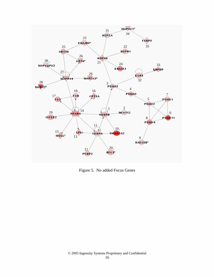
We were most interested in understanding why focus-focus edges were deleted when Focus Genes were added. For example, when a single Focus Gene was added to 225 Focus Genes (see figure 4) two Focus-Focus edges were deleted: HSPA8 – HSPCA, and PSMA3 – EGR1. We can see these edges in the IPA network when no Focus Genes were added. In the following network, the number represents the order the algorithm chose to add each gene:
© 2005 Ingenuity Systems Proprietary and Confidential 15
31 34
25
23
26
35 22
27
28
30 21 24 33
3
29
32
4 18 16 7 17
5
2
10
1
11
14 19 6 8
15 13 9
20 12
Figure 5. No added Focus Genes
© 2005 Ingenuity Systems Proprietary and Confidential 16
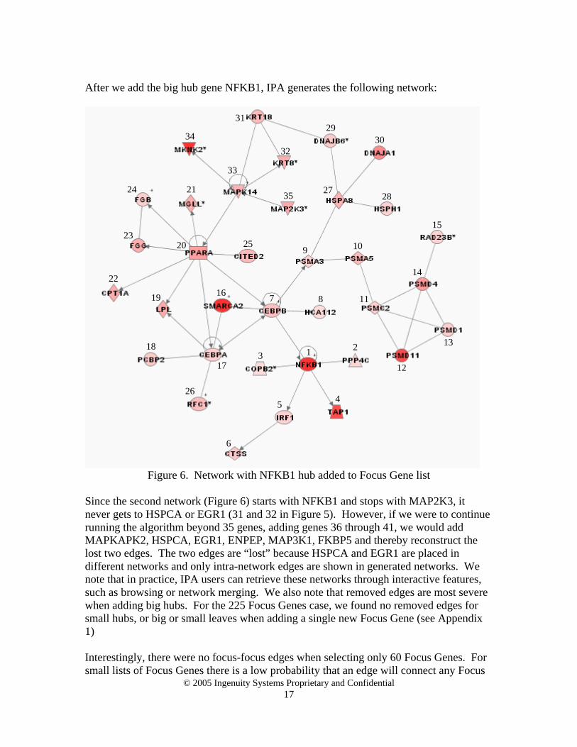
After we add the big hub gene NFKB1, IPA generates the following network:
31 29
34 30 32
33
24 21 27 35 28
15 23
25 20 10 9
14 22
16 19 7 11 8
13 18 2 1 3 17 12
26 4 5
6
Figure 6. Network with NFKB1 hub added to Focus Gene list Since the second network (Figure 6) starts with NFKB1 and stops with MAP2K3, it never gets to HSPCA or EGR1 (31 and 32 in Figure 5). However, if we were to continue running the algorithm beyond 35 genes, adding genes 36 through 41, we would add MAPKAPK2, HSPCA, EGR1, ENPEP, MAP3K1, FKBP5 and thereby reconstruct the lost two edges. The two edges are “lost” because HSPCA and EGR1 are placed in different networks and only intra-network edges are shown in generated networks. We note that in practice, IPA users can retrieve these networks through interactive features, such as browsing or network merging. We also note that removed edges are most severe when adding big hubs. For the 225 Focus Genes case, we found no removed edges for small hubs, or big or small leaves when adding a single new Focus Gene (see Appendix 1)
© 2005 Ingenuity Systems Proprietary and Confidential 17
Interestingly, there were no focus-focus edges when selecting only 60 Focus Genes. For small lists of Focus Genes there is a low probability that an edge will connect any Focus
© 2005 Ingenuity Systems Proprietary and Confidential 18
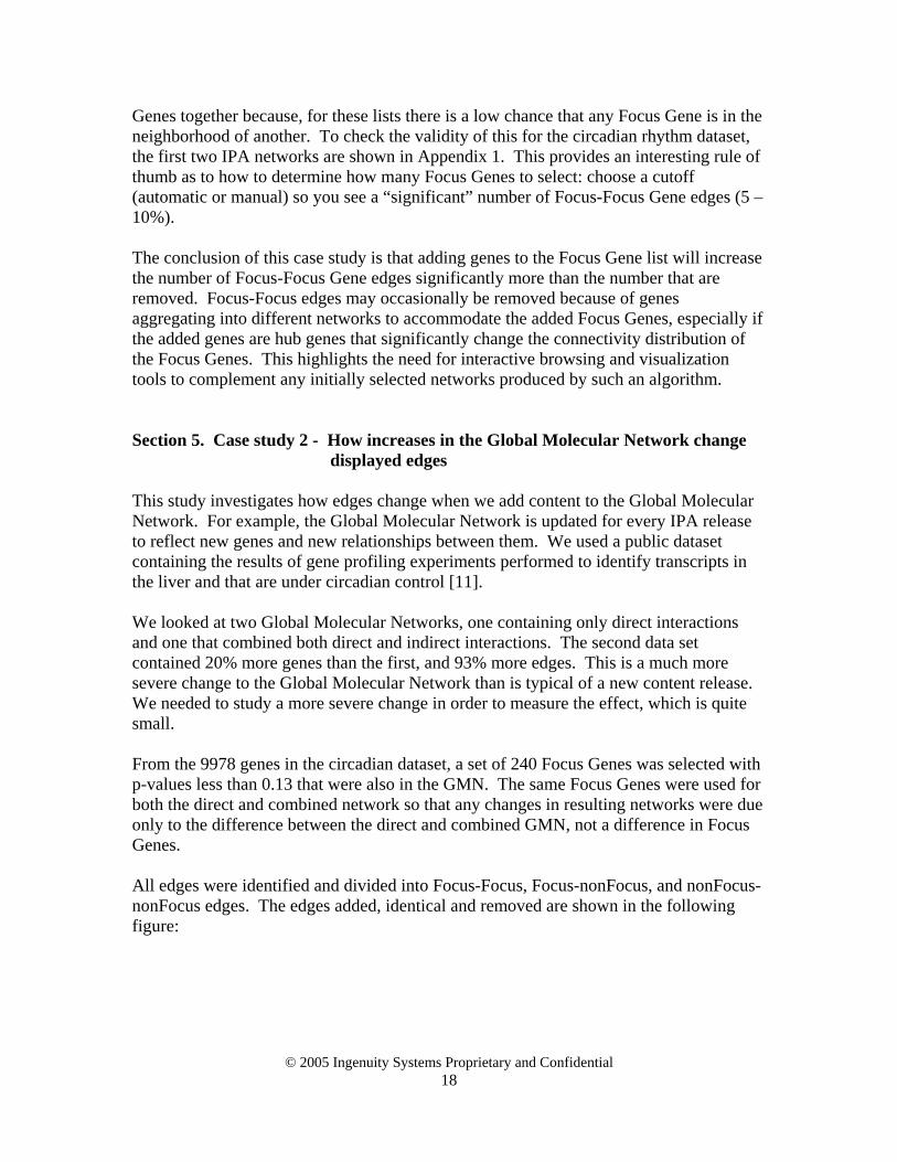
Genes together because, for these lists there is a low chance that any Focus Gene is in the neighborhood of another. To check the validity of this for the circadian rhythm dataset, the first two IPA networks are shown in Appendix 1. This provides an interesting rule of thumb as to how to determine how many Focus Genes to select: choose a cutoff (automatic or manual) so you see a “significant” number of Focus-Focus Gene edges (5 – 10%). The conclusion of this case study is that adding genes to the Focus Gene list will increase the number of Focus-Focus Gene edges significantly more than the number that are removed. Focus-Focus edges may occasionally be removed because of genes aggregating into different networks to accommodate the added Focus Genes, especially if the added genes are hub genes that significantly change the connectivity distribution of the Focus Genes. This highlights the need for interactive browsing and visualization tools to complement any initially selected networks produced by such an algorithm. Section 5. Case study 2 - How increases in the Global Molecular Network change
displayed edges This study investigates how edges change when we add content to the Global Molecular Network. For example, the Global Molecular Network is updated for every IPA release to reflect new genes and new relationships between them. We used a public dataset containing the results of gene profiling experiments performed to identify transcripts in the liver and that are under circadian control [11]. We looked at two Global Molecular Networks, one containing only direct interactions and one that combined both direct and indirect interactions. The second data set contained 20% more genes than the first, and 93% more edges. This is a much more severe change to the Global Molecular Network than is typical of a new content release. We needed to study a more severe change in order to measure the effect, which is quite small. From the 9978 genes in the circadian dataset, a set of 240 Focus Genes was selected with p-values less than 0.13 that were also in the GMN. The same Focus Genes were used for both the direct and combined network so that any changes in resulting networks were due only to the difference between the direct and combined GMN, not a difference in Focus Genes. All edges were identified and divided into Focus-Focus, Focus-nonFocus, and nonFocus-nonFocus edges. The edges added, identical and removed are shown in the following figure:
Changes due to indirect interations
0
50
100
150
200
250
300
350
400
Added Same Removed
Num
ber o
f int
erac
tions
FG - FGFG - NFGNFG - NFG
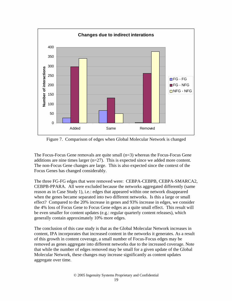
Figure 7. Comparison of edges when Global Molecular Network is changed
The Focus-Focus Gene removals are quite small (n=3) whereas the Focus-Focus Gene additions are nine times larger (n=27). This is expected since we added more content. The non-Focus Gene changes are large. This is also expected since the context of the Focus Genes has changed considerably. The three FG-FG edges that were removed were: CEBPA-CEBPB, CEBPA-SMARCA2, CEBPB-PPARA. All were excluded because the networks aggregated differently (same reason as in Case Study 1), i.e.: edges that appeared within one network disappeared when the genes became separated into two different networks. Is this a large or small effect? Compared to the 20% increase in genes and 93% increase in edges, we consider the 4% loss of Focus Gene to Focus Gene edges as a quite small effect. This result will be even smaller for content updates (e.g.: regular quarterly content releases), which generally contain approximately 10% more edges. The conclusion of this case study is that as the Global Molecular Network increases in content, IPA incorporates that increased content in the networks it generates. As a result of this growth in content coverage, a small number of Focus-Focus edges may be removed as genes aggregate into different networks due to the increased coverage. Note that while the number of edges removed may be small for a given update of the Global Molecular Network, these changes may increase significantly as content updates aggregate over time.
© 2005 Ingenuity Systems Proprietary and Confidential 19
© 2005 Ingenuity Systems Proprietary and Confidential 20
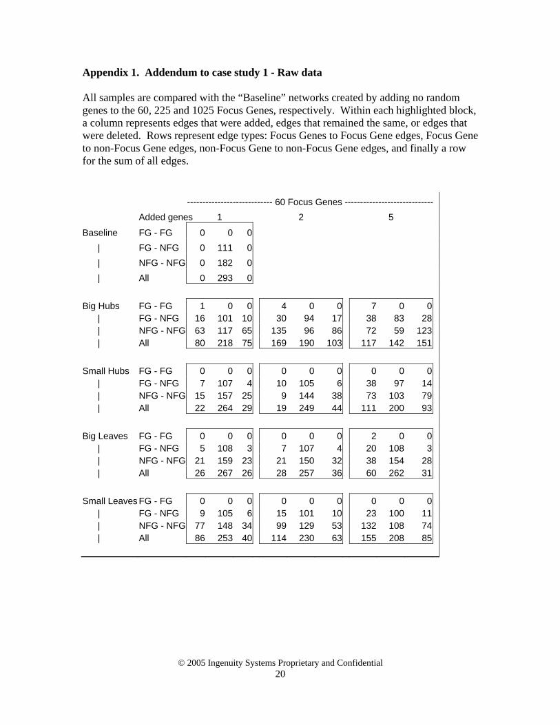
Appendix 1. Addendum to case study 1 - Raw data All samples are compared with the “Baseline” networks created by adding no random genes to the 60, 225 and 1025 Focus Genes, respectively. Within each highlighted block, a column represents edges that were added, edges that remained the same, or edges that were deleted. Rows represent edge types: Focus Genes to Focus Gene edges, Focus Gene to non-Focus Gene edges, non-Focus Gene to non-Focus Gene edges, and finally a row for the sum of all edges. ---------------------------- 60 Focus Genes ----------------------------- Added genes 1 2 5
Baseline FG - FG 0 0 0 | FG - NFG 0 111 0 | NFG - NFG 0 182 0 | All 0 293 0 Big Hubs FG - FG 1 0 0 4 0 0 7 0 0 | FG - NFG 16 101 10 30 94 17 38 83 28 | NFG - NFG 63 117 65 135 96 86 72 59 123 | All 80 218 75 169 190 103 117 142 151 Small Hubs FG - FG 0 0 0 0 0 0 0 0 0 | FG - NFG 7 107 4 10 105 6 38 97 14 | NFG - NFG 15 157 25 9 144 38 73 103 79 | All 22 264 29 19 249 44 111 200 93 Big Leaves FG - FG 0 0 0 0 0 0 2 0 0 | FG - NFG 5 108 3 7 107 4 20 108 3 | NFG - NFG 21 159 23 21 150 32 38 154 28 | All 26 267 26 28 257 36 60 262 31 Small Leaves FG - FG 0 0 0 0 0 0 0 0 0 | FG - NFG 9 105 6 15 101 10 23 100 11 | NFG - NFG 77 148 34 99 129 53 132 108 74 | All 86 253 40 114 230 63 155 208 85
© 2005 Ingenuity Systems Proprietary and Confidential 21
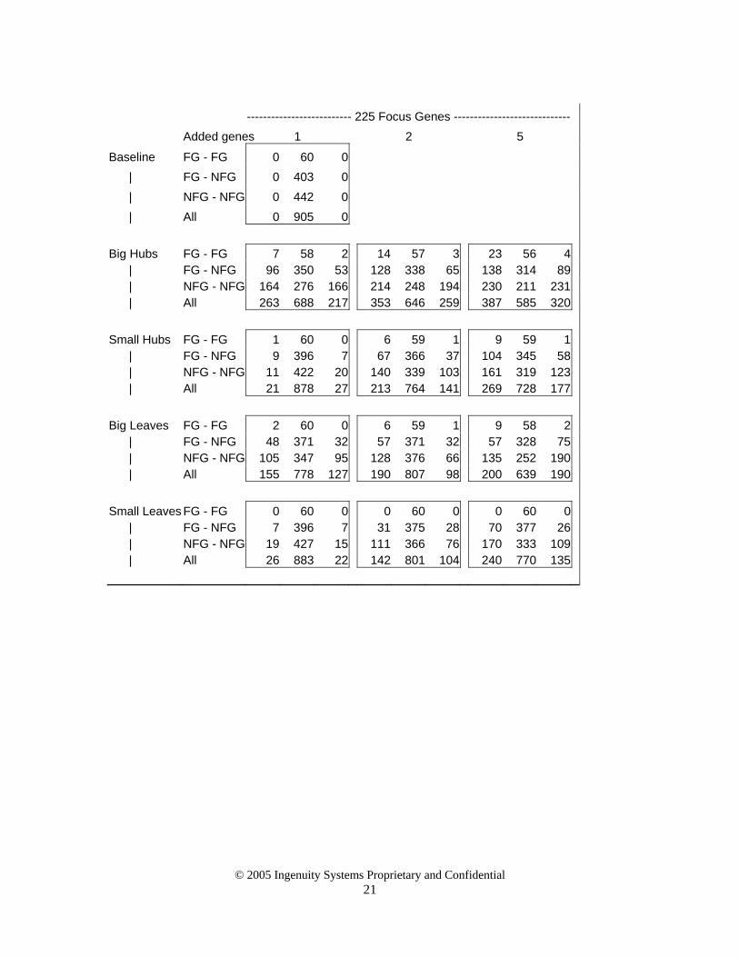
-------------------------- 225 Focus Genes ----------------------------- Added genes 1 2 5
Baseline FG - FG 0 60 0 | FG - NFG 0 403 0 | NFG - NFG 0 442 0 | All 0 905 0 Big Hubs FG - FG 7 58 2 14 57 3 23 56 4 | FG - NFG 96 350 53 128 338 65 138 314 89 | NFG - NFG 164 276 166 214 248 194 230 211 231 | All 263 688 217 353 646 259 387 585 320 Small Hubs FG - FG 1 60 0 6 59 1 9 59 1 | FG - NFG 9 396 7 67 366 37 104 345 58 | NFG - NFG 11 422 20 140 339 103 161 319 123 | All 21 878 27 213 764 141 269 728 177 Big Leaves FG - FG 2 60 0 6 59 1 9 58 2 | FG - NFG 48 371 32 57 371 32 57 328 75 | NFG - NFG 105 347 95 128 376 66 135 252 190 | All 155 778 127 190 807 98 200 639 190 Small Leaves FG - FG 0 60 0 0 60 0 0 60 0 | FG - NFG 7 396 7 31 375 28 70 377 26 | NFG - NFG 19 427 15 111 366 76 170 333 109 | All 26 883 22 142 801 104 240 770 135
© 2005 Ingenuity Systems Proprietary and Confidential 22
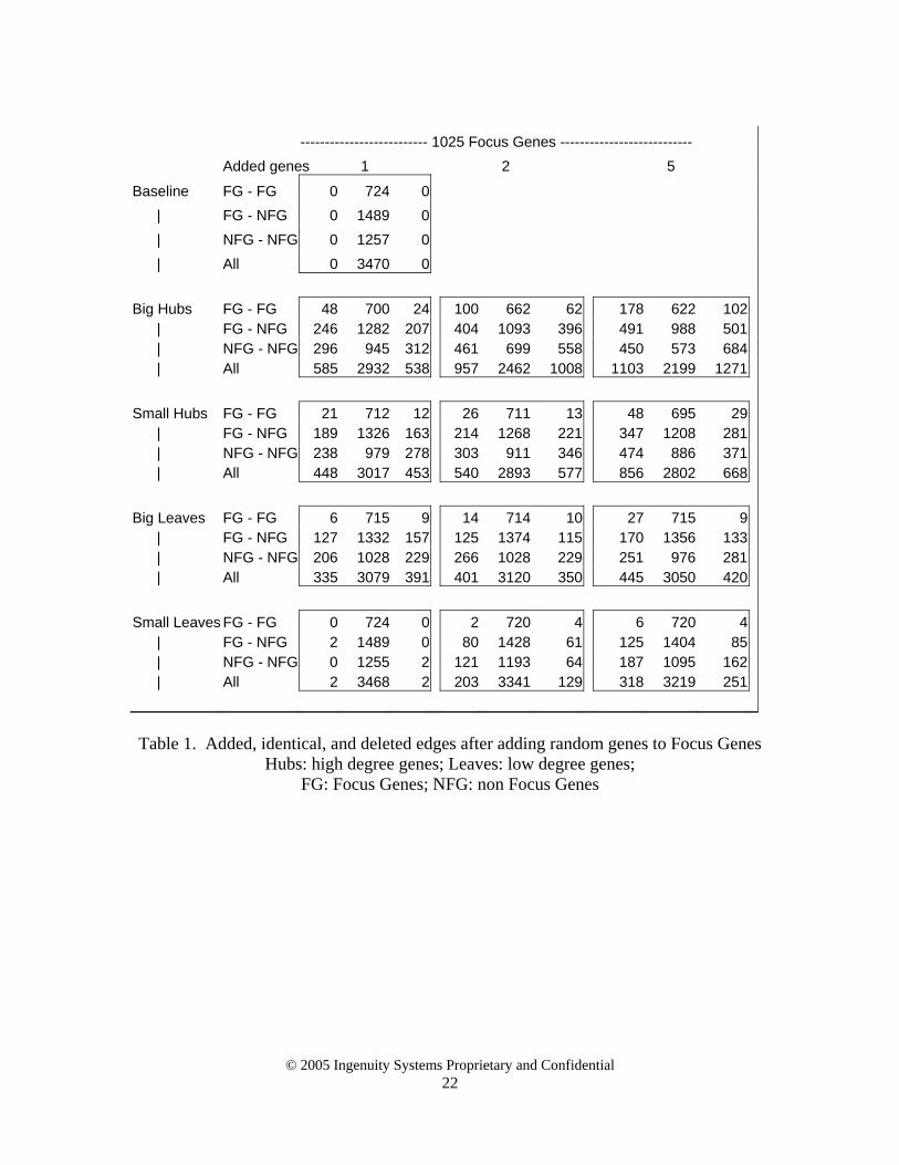
-------------------------- 1025 Focus Genes --------------------------- Added genes 1 2 5
Baseline FG - FG 0 724 0 | FG - NFG 0 1489 0 | NFG - NFG 0 1257 0 | All 0 3470 0 Big Hubs FG - FG 48 700 24 100 662 62 178 622 102 | FG - NFG 246 1282 207 404 1093 396 491 988 501 | NFG - NFG 296 945 312 461 699 558 450 573 684 | All 585 2932 538 957 2462 1008 1103 2199 1271 Small Hubs FG - FG 21 712 12 26 711 13 48 695 29 | FG - NFG 189 1326 163 214 1268 221 347 1208 281 | NFG - NFG 238 979 278 303 911 346 474 886 371 | All 448 3017 453 540 2893 577 856 2802 668 Big Leaves FG - FG 6 715 9 14 714 10 27 715 9 | FG - NFG 127 1332 157 125 1374 115 170 1356 133 | NFG - NFG 206 1028 229 266 1028 229 251 976 281 | All 335 3079 391 401 3120 350 445 3050 420 Small Leaves FG - FG 0 724 0 2 720 4 6 720 4 | FG - NFG 2 1489 0 80 1428 61 125 1404 85 | NFG - NFG 0 1255 2 121 1193 64 187 1095 162 | All 2 3468 2 203 3341 129 318 3219 251
Table 1. Added, identical, and deleted edges after adding random genes to Focus Genes
Hubs: high degree genes; Leaves: low degree genes; FG: Focus Genes; NFG: non Focus Genes
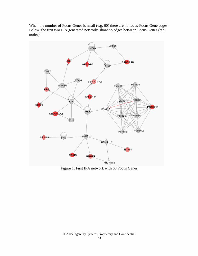
When the number of Focus Genes is small (e.g. 60) there are no focus-Focus Gene edges. Below, the first two IPA generated networks show no edges between Focus Genes (red nodes).
Figure 1: First IPA network with 60 Focus Genes
© 2005 Ingenuity Systems Proprietary and Confidential 23
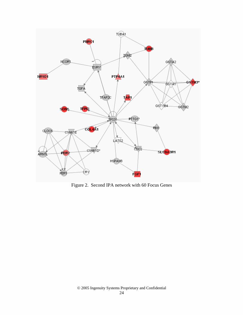
Figure 2. Second IPA network with 60 Focus Genes
© 2005 Ingenuity Systems Proprietary and Confidential 24

© 2005 Ingenuity Systems Proprietary and Confidential 25
Appendix 2. Poster presentation 2005 IEEE Computational Systems Biology Conference
Title: Functional modularity in a large-scale mammalian molecular interaction network Authors: Andreas Krämer, Daniel R. Richards, James O. Bowlby, and Ramon M. Felciano Abstract: Ingenuity™ Pathway Analysis (IPA) is a system that transforms a list of genes of interest into a set of relevant networks based on structured content from Ingenuity’s Pathways Knowledge Base (IPKB). This knowledge base contains over one million highly-structured findings manually curated from the scientific literature. The IPA algorithm uses a global molecular network of direct interactions observed between mammalian orthologs computed from the IPKB. The selection of relevant subnetworks in the IPA algorithm is based in part on the assumption that biological function correlates with locally-dense molecular interactions. In this study we validate this assumption by exploring the relationship between this global network and known functional annotations of genes. In particular we show that (a) subnetworks formed by genes annotated with the same functional category have significantly more edges than equivalent random subnetworks, and (b) highly-interconnected subnetworks are significantly enriched in genes with specific functional annotations. The statistical analysis presented here is based on a null model of random graphs that explicitly preserves the expectation values of node degrees. Highly-interconnected subnetworks are detected by maximizing the network’s modularity in replicated simulated annealing runs, and subsequently applying a hierarchical clustering method.
© 2005 Ingenuity Systems Proprietary and Confidential 26
[1] S. E. Calvano, W. Xiao, D. R. Richards, R. M. Felciano, H. V. Baker, R. J. Cho,
R. O. Chen, B. H. Brownstein, J. P. Cobb, S. K. Tschoeke, C. Miller-Graziano, L. L. Moldawer, M. N. Mindrinos, R. W. Davis, R. G. Tompkins, and S. F. Lowry, "A network-based analysis of systemic inflammation in humans," Nature, vol. 437, pp. 1032-7, 2005.
[2] D. Ficenec, M. Osborne, J. Pradines, D. Richards, R. Felciano, R. J. Cho, R. O. Chen, T. Liefeld, J. Owen, A. Ruttenberg, C. Reich, J. Horvath, and T. Clark, "Computational knowledge integration in biopharmaceutical research," Brief Bioinform, vol. 4, pp. 260-78, 2003.
[3] A. Krämer, D. R. Richards, J. O. Bowlby, and R. M. Felciano, "Functional modularity in a large-scale mammalian molecular interaction network (poster)," presented at 2005 IEEE Computational Systems Biology Conference, Stanford University, Stanford, CA, 2005.
[4] H. W. Ma, X. M. Zhao, Y. J. Yuan, and A. P. Zeng, "Decomposition of metabolic network into functional modules based on the global connectivity structure of reaction graph," Bioinformatics, vol. 20, pp. 1870-6, 2004.
[5] E. Ravasz, A. L. Somera, D. A. Mongru, Z. N. Oltvai, and A. L. Barabasi, "Hierarchical organization of modularity in metabolic networks," Science, vol. 297, pp. 1551-5, 2002.
[6] V. Spirin and L. A. Mirny, "Protein complexes and functional modules in molecular networks," Proc Natl Acad Sci U S A, vol. 100, pp. 12123-8, 2003.
[7] T. Ideker, O. Ozier, B. Schwikowski, and A. F. Siegel, "Discovering regulatory and signalling circuits in molecular interaction networks," Bioinformatics, vol. 18 Suppl 1, pp. S233-40, 2002.
[8] D. Rajagopalan and P. Agarwal, "Inferring pathways from gene lists using a literature-derived network of biological relationships," Bioinformatics, vol. 21, pp. 788-93, 2005.
[9] J. Pradines, L. Rudolph-Owen, J. Hunter, P. Leroy, M. Cary, R. Coopersmith, V. Dancik, Y. Eltsefon, V. Farutin, C. Leroy, J. Rees, D. Rose, S. Rowley, A. Ruttenberg, P. Wieghardt, C. Sander, and C. Reich, "Detection of activity centers in cellular pathways using transcript profiling," J Biopharm Stat, vol. 14, pp. 701-21, 2004.
[10] G. D. Bader and C. W. Hogue, "An automated method for finding molecular complexes in large protein interaction networks," BMC Bioinformatics, vol. 4, pp. 2, 2003.
[11] S. Panda, M. P. Antoch, B. H. Miller, A. I. Su, A. B. Schook, M. Straume, P. G. Schultz, S. A. Kay, J. S. Takahashi, and J. B. Hogenesch, "Coordinated transcription of key pathways in the mouse by the circadian clock," Cell, vol. 109, pp. 307-20, 2002.