* Communications Architectures and Research Section.

† Tracking Systems and Applications Section.

The research described in this publication was carried out by the Jet Propulsion Laboratory, California Institute of Technology, under a contract with the National Aeronautics and Space Administration. © 2020 California Institute of Technology. U.S. Government sponsorship acknowledged. 1

IPN Progress Report 42-222 • August 15, 2020

Radar Study of Inactive Geosynchronous Earth Orbit Satellite Spin States

Conor J. Benson,* Charles J. Naudet,† and Stephen T. Lowe†

ABSTRACT. — The growing inactive satellite population near geosynchronous Earth orbit (GEO) motivates improved understanding of these satellites’ dynamical evolution. Proposed active debris removal and servicing missions will require accurate spin state knowledge and predictions to capture and de-spin these large, inactive satellites. Spin state estimation from ubiquitous non-resolved ground-based optical measurements is very challenging due to complex satellite geometry and reflections. In this paper, we investigate how spin state estimates can be achieved through radar observations of inactive GEO satellites by the Deep Space Network (DSN). Leveraging time-varying viewing geometry due to Earth’s rotation and limited satellite geometry knowledge, we find that we can greatly constrain a satellite’s inertial spin pole. Analysis of 2017 Doppler echoes for the Echostar 2 satellite yielded pole solutions consistent with earlier optical studies. In addition, we have developed a radar observation model and unscented batch filter for radar-based spin state estimation.

I. Introduction

Inactive GEO satellites have diverse and evolving spin rates [1,2,3], but limited research has been conducted to better understand this behavior [3,4,5,6]. Meanwhile, extensive research has been done on asteroid spin dynamics subject to the solar radiation torques (i.e., the Yarkovsky–O'Keefe–Radzievskii–Paddack (YORP) effect) and internal energy dissipation [7,8,9,10,11]. Inactive GEO satellites are affected by similar perturbations, but their spin states change much more rapidly (months to years vs. 103 to >109 years). Therefore, inactive GEO satellites provide convenient test subjects for investigating asteroid evolution theories. In addition to asteroid applications, a better understanding of inactive satellite spin dynamics will help predict shedding of high area-to-mass ratio (HAMR) objects, aiding in active debris removal and satellite servicing missions. Accurate spin state predictions are needed to capture and de-spin large, non-cooperative GEO satellites.

2

In 2018, Albuja et al. [12] closely predicted the observed spin rate evolution of two inactive GEO satellites with a physics-based YORP model. Albuja et al. also hypothesized that satellites may cycle indefinitely between phases of uniform rotation and multi-axis tumbling due to YORP and internal energy dissipation. In addition to further modeling of YORP, dissipation, gravity gradients, and magnetic torques, observations of inactive satellites are needed to understand this tumbling motion and form a better picture of long-term spin state evolution. Recent simulations suggest that YORP-driven tumbling is strongly dictated by the inertial direction of the satellite’s rotational angular momentum vector, which has a tendency to track the time-varying Sun direction [3]. The angular momentum direction (i.e., pole) is difficult to estimate from optical light curve observations alone, even for satellites with well-documented geometry and pre-launch optical properties. This is largely due to the fact that GEO satellites are not resolvable with ground-based optical telescopes. These satellites exhibit frequent specular reflections from symmetric surfaces, often resulting in many well-fitting pole solutions.

II. Doppler Data

We investigate this pole estimation problem by analyzing Goldstone Doppler data of inactive GEO satellites collected during the JPL Multi-Static Radar Demonstration (MRD) in 2017 [13]. Doppler echoes were obtained using a bi-static configuration, transmitting continuous wave (cw) carrier signals from DSS-26 to the target satellites and receiving the echoes at DSS-13. Transmit power was 80 kW and three slightly different transmit frequencies were used: 1) 7.148 GHz, 2) 7.164 GHz, and 3) 7.185 GHz. The resulting echoes were processed with a windowed Fast Fourier Transform (FFT). The FFT integration time was manually adjusted to compromise between low rotational smear and high frequency resolution given each target’s observed spin period. The rotation-driven Doppler was then isolated by subtracting the predicted orbital Doppler calculated with JPL Horizons ephemerides. The inactive GEO satellites observed for MRD included Echostar 2 and Telstar 401.

Sample Doppler echoes for Telstar 401 are provided in Figure 1 with brighter points corresponding to higher echo power. The echoes show clear periodicity indicating principal axis rotation. The outer extents likely correspond to the satellite’s two solar panels, and the bright inner sections to the satellite bus. The outer extents have alternating

Figure 1. Telstar 401 Doppler (time relative to March 2, 2017 05:05:05 UTC).

3

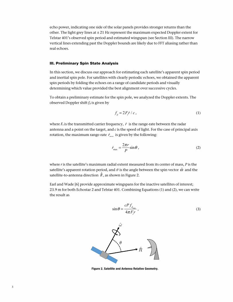
echo power, indicating one side of the solar panels provides stronger returns than the other. The light grey lines at ± 21 Hz represent the maximum expected Doppler extent for Telstar 401’s observed spin period and estimated wingspan (see Section III). The narrow vertical lines extending past the Doppler bounds are likely due to FFT aliasing rather than real echoes.

III. Preliminary Spin State Analysis

In this section, we discuss our approach for estimating each satellite’s apparent spin period and inertial spin pole. For satellites with clearly periodic echoes, we obtained the apparent spin periods by folding the echoes on a range of candidate periods and visually determining which value provided the best alignment over successive cycles.

To obtain a preliminary estimate for the spin pole, we analyzed the Doppler extents. The observed Doppler shift fd is given by

, (1)

where Ft is the transmitted carrier frequency, is the range-rate between the radar antenna and a point on the target, and c is the speed of light. For the case of principal axis rotation, the maximum range-rate is given by the following:

, (2)

where r is the satellite’s maximum radial extent measured from its center of mass, P is the satellite’s apparent rotation period, and q is the angle between the spin vector and the satellite-to-antenna direction , as shown in Figure 2.

Earl and Wade [6] provide approximate wingspans for the inactive satellites of interest; 23.9 m for both Echostar 2 and Telstar 401. Combining Equations (1) and (2), we can write the result as

, (3)

fd = 2Ft !r / c

!r

!rmax

!rmax =2πrPsinθ

ω̂R̂

sinθ =cP fdmax4πFtr

Figure 2. Satellite and Antenna Relative Geometry.

4

where is maximum observed Doppler extent (i.e., amplitude). This equation is

essentially the ratio of and the maximum expected Doppler when the spin pole and

line of sight are perpendicular to each other (q = 90°). The maximum magnitude of the expected Doppler for Telstar 401 is shown as the two horizontal grey lines in Figure 1.

A given value of sinq provides two possible cones on which lies (only one cone if

q = 90°). Echoes obtained from other viewing directions provide additional values for sin q. Viable solutions must lie on the intersection of cones from all observation epochs. Near

GEO, moves roughly 15° per hour in inertial space. With a bi-static radar configuration,

the well-spaced directions can be obtained by observing the target every several hours or at different local times on subsequent days, assuming spin pole motion is negligible.

A. Telstar 401

Analysis of the Telstar 401 Doppler echoes revealed a spin period of ~169 s. This is close to the ~158 s spin period reported by Earl and Wade [6]. Figure 3 shows the normalized echoes for February 23 and March 2, 2017, days of year (DOY) 54 and 61, respectively. The five frames in Figure 3 are provided in chronological order. We obtained these echoes by dividing the observed Doppler by Telstar 401’s maximum expected Doppler at the corresponding transmit frequency. For MRD, the three transmit frequencies were broadcast on sequential tracks, resulting in slightly different observation geometries on a given day. In the first three frames in Figure 3, we can see the observed Doppler extent increase during DOY054. The extent is then largest on DOY061 (Figure 3d and 3e) and very close to the maximum expected value. Calculating q from the maximum extent for each of the five epochs, we found approximate values of 65°/115°, 70°/110°, 80°/100°, 90°, and 90°, respectively.

Figure 4 shows the possible spin pole cones for all five epochs plotted in the International Celestial Reference Frame (ICRF)/Julian (J)2000 equatorial frame. Figure 4a also includes the corresponding vectors. Ideally, the correct spin pole will lie at the intersection of cones for all five epochs. The two most consistent spin pole solutions have longitude (right ascension) = 240° ± 10°, latitude (declination) = 40° ± 10°, and longitude = 60° ± 10°, latitude = –40° ± 10°. The two regions near the north and south poles are likely not viable solutions given their poor cone intersection.

fdmaxfdmax

ω̂

R̂R̂

R̂

(a) (b) (c) (d) (e)

Figure 3. Telstar 401 Normalized Doppler Echoes on February 23 (DOY054) and March 2 (DOY061) 2017.

5

B. Echostar 2

By phase-folding the Echostar 2 Doppler, we obtained well-fitted periods of 511 s–523 s at the different observation epochs. Earl and Wade [6] reported an average spin period of ~439 s for their observations in 2012–2013, indicating a notable change in spin rate over this time. Figure 5 shows the Doppler echoes for March 2, 2017, folded on the best-fitted 522.6 s period. The maximum expected Doppler extents of 6.9 Hz are also plotted. The real Doppler extents follow a sinusoidal pattern, while the narrow vertical lines extending beyond this sinusoid are likely due to aliasing. The two bright signatures at ~90 s and ~350 s correspond to the solar array axis when it is perpendicular to the radar line of sight. Additional symmetric features are also present on either side of these maximum Doppler extents. These potentially correspond to the pair of bus-mounted communication antennas.

Echoes obtained on DOY054, DOY061, and DOY062 all showed observed Doppler extents approximately equal to the maximum expected values, indicating q ≈ 90° on all three days. Plotting the possible spin pole directions, Figure 6 shows that the two consistent solutions are nearly along Earth’s north and south geographic pole, respectively. Independent optical glint analysis by Earl et al. [14] suggests Echostar 2’s spin pole is within 30° of either geographic pole, agreeing with the radar-derived solutions.

(a) (b)

Figure 4. Telstar 401 Spin Pole Estimate (ICRF/J2000).

Figure 5. Echostar 2 Period-Folded Doppler Echoes (March 2, 2017).

6

IV. Radar Observation Model

To further analyze the MRD observations, we developed a simple facet-based radar observation model. The Telstar 401 model is provided in Figure 7 and consists of ~1400 facets. The bus (gold), solar arrays (blue), and antennas (gray) are included in the radar shape model. Approximate model dimensions were taken from Earl et al. [14].

Simulated echoes are calculated with the following approach. The range to the ith satellite facet ri is computed with the following equations, where is the position vector from the satellite center of mass to the facet centroid, and is the vector from the satellite center of mass to the radar antenna (calculated using JPL Navigation and Ancillary Information Facility (NAIF) Spacecraft, Planet, Instrument, C-matrix, Events (SPICE)1 ephemerides). Note that is rotated from J2000 to the satellite-fixed frame.

(4)

(5)

The facet’s range-rate is then calculated with the following, assuming :

, (6)

where is the satellite’s inertial angular velocity and is the inertial

rate of change of . Both and the orbital range-rate can be calculated from the

1 JPL Navigation and Ancillary Information Facility SPICE Toolkit, https://naif.jpl.nasa.gov/naif/

!ci!R = RR̂

R̂

!ri =!R − !ci

ri =!ri

!ri!ci ≪

!R

!ri = −"ω −"ω R/N( )× "ci⎡⎣ ⎤⎦ ⋅ R̂ + !R

!ω!ω R/N = − 1

R!"R × "R

R̂ !ω R/N!R

(a) (b)

Figure 6. Echostar 2 Spin Pole Estimate (ICRF/J2000).

7

(a)

(b)

Figure 7. (a) Telstar 401 Illustration (Lockheed Martin); (b) Telstar 401 Radar Shape Model.

satellite’s known orbit. The spacecraft attitude and were obtained by numerically integrating Euler’s torque free rigid body equations of motion and the quaternion kinematic differential equations [15]. The echo power of each facet Pi is given by

where is the facet radar cross section and is a constant scaling factor

(for analyzing the observations given in dB above the noise). For this simple model, is

given by:

. (7)

Here, r i is the facet reflectivity, Ai is its area, and is its outward unit normal vector. The max() function ensures that facets only provide echoes when is above the facet plane. Finally, ki is a constant that controls the backscatter law (e.g., corresponds to Lambertian reflection and to a purely specular glint). For this model, no self-shadowing, multi-bounce, or induced current behavior is considered. To obtain Doppler-delay images, the facet power is then binned into delay and Doppler bins. Since the MRD data did not include ranging, only simulated Doppler observations were analyzed.

Figure 8 shows simulated Doppler echoes for Telstar 401. Note the similarity to the observed Telstar 401 echoes in Figure 1 (the start time in Figure 8 is arbitrary and unrelated to that in Figure 1). Here, we assumed the reflectivity of all facets to be equal. Nevertheless, the echo power from the front and back of the solar array differs because normally and the solar array are both inclined to the satellite’s equatorial plane, so one side of the array has a larger projected area than the other. In addition to differing reflectivity, this could explain the echo power differences in Figure 1. Also visible in Figure 8 is the smaller bandwidth oscillations due to the satellite bus and two antennas. These are similar to features in Figure 1. One notable difference between the simulated and observed echoes is the lack of returns between the bus and solar array in Figure 8. Obviously, this is due to omission of the solar array mounting arms from the simple shape model (Figure 7b). Nevertheless, given the space between the mounting arms, one would also expect lower echo power in this region in Figure 1, but there is no evidence of that. This suggests that either the frequency resolution is not fine enough to resolve these gaps in Figure 1, or that RF-induced currents in the solar array mounting arms supplement the echo power. There are two dots with a notable increase in echo power located at ~±5 Hz at times of maximum

!ω

Pi = Csfσ i σ i Csfσ i

σ i = ρi Aimax r̂i ⋅ n̂i ,0( )ki

n̂ir̂iki = 2

ki →∞

R̂

8

extent in Figure 1. These dots are near the mounting arm locations, supporting the latter explanation.

V. Batch Filter Spin State Estimation

An estimation filter was required to estimate a satellite’s complete spin state (attitude and angular velocity) at a given epoch (in addition to parameters such as the body-frame spin axis and solar array angle). The commonly used batch and Kalman filters require partial derivatives of the observations (i.e., the delay-Doppler images) with respect to the estimated state (i.e., spin state and other parameters). To analytically obtain the observation partials, one would need to approximate the unit impulse binning function with an analytical function. We decided not to use this approach, given the large derivatives and resulting numerical issues associated with impulse approximation functions. So, we investigated gradient-free approaches.. Initially, we explored using an Unscented Kalman Filter (UKF). The UKF is a sequential filter that updates the estimated state after each observation time. Unlike batch and conventional Kalman filters, the covariance and Kalman gain are calculated using specifically chosen sigma points. This makes state transition matrices and observation partials unnecessary.

Unfortunately, testing with simulated observations showed that the sequential nature of the UKF is incompatible with bi-static radar GEO spin state estimation. Since there is an infinite number of equally viable spin poles for the line of sight at a given time, there was a strong tendency for the UKF estimate to drift away from the truth. A filter was needed where the entire observation arc is processed before updating the state, making use of the time-varying line of sight. Ultimately, we chose the gradient-free unscented batch filter introduced by Park et al. [16]. This unscented batch filter uses sigma points similar to the UKF, but is non-sequential and only updates the state after all measurements in an arc have been processed.

For this work, the estimated state consisted of the satellite attitude and angular velocity in addition to the body-frame spin axis (maximum principal inertia axis) and body-frame solar array angle. The estimated attitude was described with Modified Rodrigues Parameters (MRPs); a minimal 3-coordinate set [15]. We used MRPs instead of quaternions to avoid the quaternion normality constraint. We took a multiplicative MRP approach in

Figure 8. Simulated Telstar 401 Doppler Echoes.

9

which the attitude was measured with respect to the current reference attitude rather than the inertial frame [15]. This helps keep the sigma points away from the ±360° MRP singularity and normalizes the attitude covariance for all reference attitudes. The MRP norm increases towards infinity as one approaches ±360°, so a prescribed MRP uncertainty would correspond to a different angular uncertainty depending on the reference attitude if the estimated MRP is with respect to the inertial frame. The sigma points were propagated using quaternions to avoid having to switch between the regular and shadow MRP sets during numerical integration.

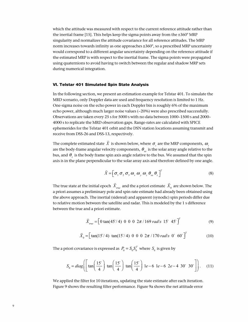
VI. Telstar 401 Simulated Spin State Analysis

In the following section, we present an estimation example for Telstar 401. To simulate the MRD scenario, only Doppler data are used and frequency resolution is limited to 1 Hz. One-sigma noise on the echo power in each Doppler bin is roughly 6% of the maximum echo power, although much larger noise values (~20%) were also prescribed successfully. Observations are taken every 25 s for 5000 s with no data between 1000–1500 s and 2000–4000 s to replicate the MRD observation gaps. Range-rates are calculated with SPICE ephemerides for the Telstar 401 orbit and the DSN station locations assuming transmit and receive from DSS-26 and DSS-13, respectively.

The complete estimated state is shown below, where are the MRP components, are the body-frame angular velocity components, is the solar array angle relative to the bus, and is the body frame spin axis angle relative to the bus. We assumed that the spin axis is in the plane perpendicular to the solar array axis and therefore defined by one angle.

(8)

The true state at the initial epoch and the a priori estimate are shown below. The a priori assumes a preliminary pole and spin rate estimate had already been obtained using the above approach. The inertial (sidereal) and apparent (synodic) spin periods differ due to relative motion between the satellite and radar. This is modeled by the 1 s difference between the true and a priori estimate.

(9)

(10)

The a priori covariance is expressed as where is given by

. (11)

We applied the filter for 10 iterations, updating the state estimate after each iteration. Figure 9 shows the resulting filter performance. Figure 9a shows the net attitude error

!X σ i ω i

θsaθ z

!X = σ 1 σ 2 σ 3ω x ω y ω z θsa θ z⎡⎣ ⎤⎦

T

!Xtrue

!X0

!Xtrue = 0 tan(45"/ 4) 0 0 0 2π / 169 rad/s 15" 45"⎡⎣ ⎤⎦

T

!X0 = tan(15"/ 4) tan(15"/ 4) 0 0 0 2π / 170 rad/s 0" 60"⎡⎣ ⎤⎦

T

P0 = S0S0T S0

S0 = diag tan 15!

4⎛⎝⎜

⎞⎠⎟ tan

15!

4⎛⎝⎜

⎞⎠⎟ tan

15!

4⎛⎝⎜

⎞⎠⎟ 1e− 6 1e− 6 2e− 4 30

! 30!⎡

⎣⎢

⎤

⎦⎥

⎛⎝⎜

⎞⎠⎟

10

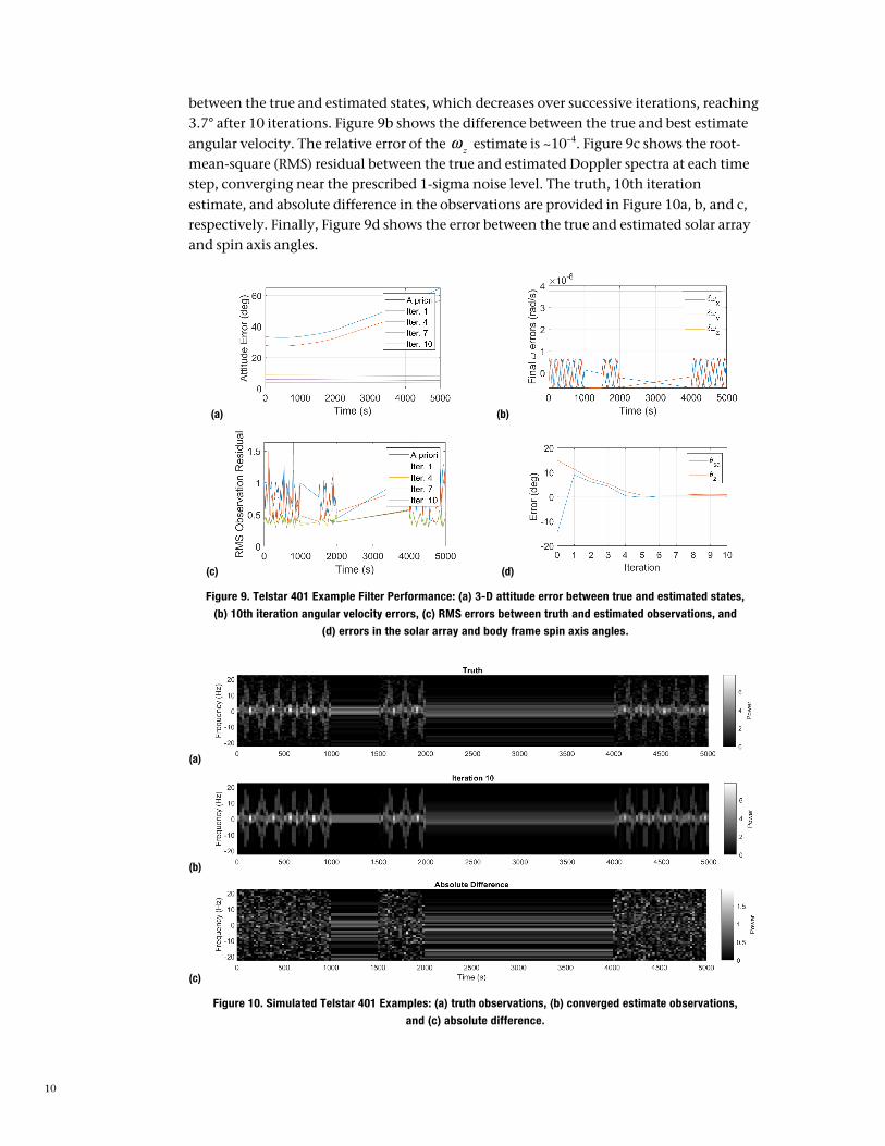
between the true and estimated states, which decreases over successive iterations, reaching 3.7° after 10 iterations. Figure 9b shows the difference between the true and best estimate angular velocity. The relative error of the estimate is ~10–4. Figure 9c shows the root-mean-square (RMS) residual between the true and estimated Doppler spectra at each time step, converging near the prescribed 1-sigma noise level. The truth, 10th iteration estimate, and absolute difference in the observations are provided in Figure 10a, b, and c, respectively. Finally, Figure 9d shows the error between the true and estimated solar array and spin axis angles.

(a) (b)

(c) (d)

Figure 9. Telstar 401 Example Filter Performance: (a) 3-D attitude error between true and estimated states,

(b) 10th iteration angular velocity errors, (c) RMS errors between truth and estimated observations, and

(d) errors in the solar array and body frame spin axis angles.

(a)

(b)

(c)

Figure 10. Simulated Telstar 401 Examples: (a) truth observations, (b) converged estimate observations,

and (c) absolute difference.

ω z

11

VII. Telstar 401 Real Spin State Analysis

After completing the Telstar 401 test case above, we analyzed the real Doppler echoes with the batch filter. To facilitate analysis, we removed the vertical sinc function aliases and residual Doppler from imprecise orbital ephemerides. The echo power, provided in dB above the noise, was converted to a linear scale and binned in 1 Hz bins for comparison with the simulated radar model. We considered the DOY054 data, with 50 observations taken over a ~3000 s arc.

We estimated the satellite’s complete spin state (attitude and angular velocity) along with

its body-frame spin axis and solar array angles, the bus reflectivity , the solar array front

and back reflectivities and , and . This is a total of 12 parameters. Since

q ≈ 90° towards the end of the DOY054 arc (i.e., the radar line of sight is in the satellite equatorial plane), both the front and back of the solar array will have nearly identical projected area regardless of solar array rotation angle. Therefore, different radar reflectivities were needed to account for the echo power discrepancy between the front and back of the array in the observations (Figure 1). In addition, the model solar arrays were extended to the bus to remove the gaps present in Figure 8.

Using the preliminary spin pole estimates from Figure 4 and folded spin period, the remaining parameters were manually adjusted for consistency with the observations. We chose scattering law power ki of 2 for the solar arrays (Lambertian scattering) and a value of 4 for the bus and antennas (which approximated the observed change in echo power over rotational phase). We set relatively small a priori uncertainties to prevent diverging from the well-fitted a priori estimate with ±3σ values of 15° for the attitude, spin axis, and solar array angles, 1.5 s for the spin period, and 0.03 for the reflectivities. The x and y axis uncertainties were made three orders of magnitude smaller given the clear principal axis spin.

After running the filter with this initial estimate, it became clear that we needed different measurement uncertainties, given the large discrepancy between the solar array and bus echo power (roughly one to two orders of magnitude weaker for the solar array). The filter would ignore observations associated with the solar arrays, and the simulated outer extents would drift away from the truth. So, we prescribed lower uncertainty for outer extents ~2% (vs. 10% for inner bus sections) to better constrain the pole and spin period. With these inputs, we obtained the solution provided in Figure 11. Given the well-fitted a priori estimates, the filter converges on a spin pole with J2000 right ascension (longitude) of 234° and equatorial declination (latitude) of 41° (see Figure 11b). The spin period (see Figure 11d) also converged to a slightly shorter value than the apparent spin period, consistent with prograde rotation of the associated spin pole. The RMS observation residual (see Figure 11a), given in dB, does not strictly decrease as this is not a least-squares filter.

Figure 12 shows the best-fit simulated observations along with the truth and difference in dB. The subtle increase in maximum extent is replicated along with the alternating echo power from the front and back of the solar array. Features and relative echo power of the bus are also comparable.

ρbρsa f ρsab Csf

12

(a) (b) (c)

(d) (e) (f)

Figure 11. Telstar 401 Spin State Estimates: (a) RMS observation residual, (b) ICRF/J2000 pole, (c) solar array

and body frame spin axis angles, (d) inertial (sidereal) spin period, (e) scale factor, and (f) reflectivity

parameters.

(a)

(b)

(c)

Figure 12. Telstar 401 Observations: (a) observed truth, (b) estimate, and (c) absolute difference (time relative to

February 23, 2017 12:20:31 UT) (Power in dB).

VIII. Discussion and Conclusions

This work demonstrates that the spin poles of GEO satellites in principal axis rotation can be greatly constrained with Doppler observations, providing reasonably accurate

13

knowledge of the satellite’s size (i.e., maximum radial extent), and two or more well-spaced inertial viewing directions of the spin axis. The latter can be achieved with multiple receiving antennas, or more efficiently by using just one antenna and taking observations spaced over the course of the day. Ideally, this approach will provide the spin pole with a 180° direction ambiguity. Complications arise in accurately measuring the maximum Doppler extent. Accurate orbital Doppler predicts are needed to separate the observed translational Doppler from the rotational Doppler. Receiver noise also makes the Doppler extent uncertain. A trade-off between Doppler and temporal resolution must also be made, as Doppler resolution is dictated by the signal integration time. Finer frequency resolution results in more rotational smear. Adding ranging might help resolve some of the peak ambiguities, but this could be the focus of future study.

With a reasonably accurate shape model, it is also possible to constrain the satellite’s body-frame spin axis (maximum inertia axis). Satellites like Telstar 401 with several bus protrusions and antennas are particularly amenable to spin axis estimation, given the Doppler shift of these features. Constraints on the body-frame solar array angle can also be made, but depend heavily on the radar backscatter law. Distinguishing the influences of the reflectivity parameters from the array’s projected area is likely to be difficult otherwise. It is possible that the array provides very similar returns over a wide range of viewing directions (i.e., face-on vs. edge on).

We achieved spin pole and rotation period estimates for the inactive GEO satellites Telstar 401 and Echostar 2 from DSN Doppler observations. Furthermore, we obtained estimates of the body-frame spin axis and additional parameters for Telstar 401. The Echostar 2 solution was consistent with independent analysis provided by Earl et al. [14]. In the future, an improved radar scattering law and further analysis of the multi-axis tumbling case are needed. Targets with less uncertainty in their dimensions and geometry would also facilitate analysis. Considering the multi-axis tumbling case, readily obtained optical light curve data could be supplemented with Doppler measurements to resolve tumbling period ambiguities and constrain the satellite’s angular momentum direction. Further radar and optical analysis would help provide insight about the ongoing spin state evolution of inactive Earth satellites.

Acknowledgments

The authors thank David Morabito for his detailed and valuable review of this paper, and Lawrence Snedeker and the entire DSS-13 technical staff for supporting this experiment.

References

[1] P. Papushev, Y. Karavaev, M. Mishina, Investigations of the evolution of optical characteristics and dynamics of proper rotation of uncontrolled geostationary artificial satellites, Advances in Space Research, vol. 43, pp. 1416–1422, 2009.

14

[2] C. J. Benson, D. J. Scheeres, W. H. Ryan, E. V. Ryan, Cyclic complex spin state evolution of defunct GEO satellites, Proceedings of the 19th Advanced Maui Optical and Space Surveillance Technologies Conference, Maui, HI, 2018.

[3] C. J. Benson, D.J. Scheeres, W. H. Ryan, E. V. Ryan, N. A. Moskovitz, GOES spin state diversity and the implications for GEO debris mitigation, Acta Astronautica, vol. 167, pp. 212–221, 2019.

[4] J. V. Fedor, The effect of solar radiation pressure on the spin of Explorer VII, NASA Goddard Space Flight Center, NASA-TN-D-1855, 1963.

[5] E. Harvie, A. Dress, M. Phenneger, GOES on-orbit storage mode attitude dynamics and control, Advances in the Astronautical Sciences, vol. 103(2), pp.1095–1114, 1999.

[6] M. A. Earl, G. A. Wade, Observations of the Spin-Period Variations of Inactive Box-Wing Geosynchronous Satellites, Journal of Spacecraft and Rockets, vol. 52 (3), pp. 968–977, 2015.

[7] D. Rubincam, Radiative spin-up and spin-down of small asteroids, Icarus, vol. 148, pp. 2–11, 2000.

[8] D. J. Scheeres, The dynamical evolution of uniformly rotating asteroids subject to YORP, Icarus, vol. 188, pp. 430–450, 2007.

[9] S. Lowry, et al., Direct detection of the asteroidal YORP effect, Science, vol. 316, pp. 272–274, 2007.

[10] D. Vokrouhlicky, S. Breiter, D. Nesvorny, W. F. Bottke, Generalized YORP evolution: Onset of tumbling and new asymptotic states, Icarus, vol. 191, pp. 636–650, 2007.

[11] S. Breiter, M. Murawiecka, Tumbling asteroid rotation with the YORP torque and inelastic energy dissipation, Monthly Notices of the Royal Astronomical Society, vol. 449, pp. 2489–2497, 2015.

[12] A. A. Albuja, D. J. Scheeres, R. L. Cognion, W. H. Ryan, E. V. Ryan, The YORP effect on the GOES 8 and GOES 10 satellites: A case study, Advances in Space Research, vol. 61, pp. 122–144, 2018.

[13] J. Breidenthal, et al., Multi-static radar demonstration FY17 final report, Jet Propulsion Laboratory Communications, Tracking and Radar Division, 2017.

[14] M. A. Earl, et al., Estimating the spin axis orientation of the Echostar-2 box-wing geosynchronous satellite, Advances in Space Research, vol. 61, pp. 2135–2146, 2018.

[15] H. Schaub, J. L. Junkins, Analytical Mechanics of Space Systems, 3rd Ed., American Institute of Aeronautics and Astronautics, Reston, VA, 2014.

[16] E. Park, S. Park, K. Roh, K. Choi, Satellite orbit determination using a batch filter based on the unscented transformation, Aerospace Science and Technology, vol. 14, pp. 387–396, 2010.

JPL CL # 29-1774