Iron and Biogeochemical Cycles

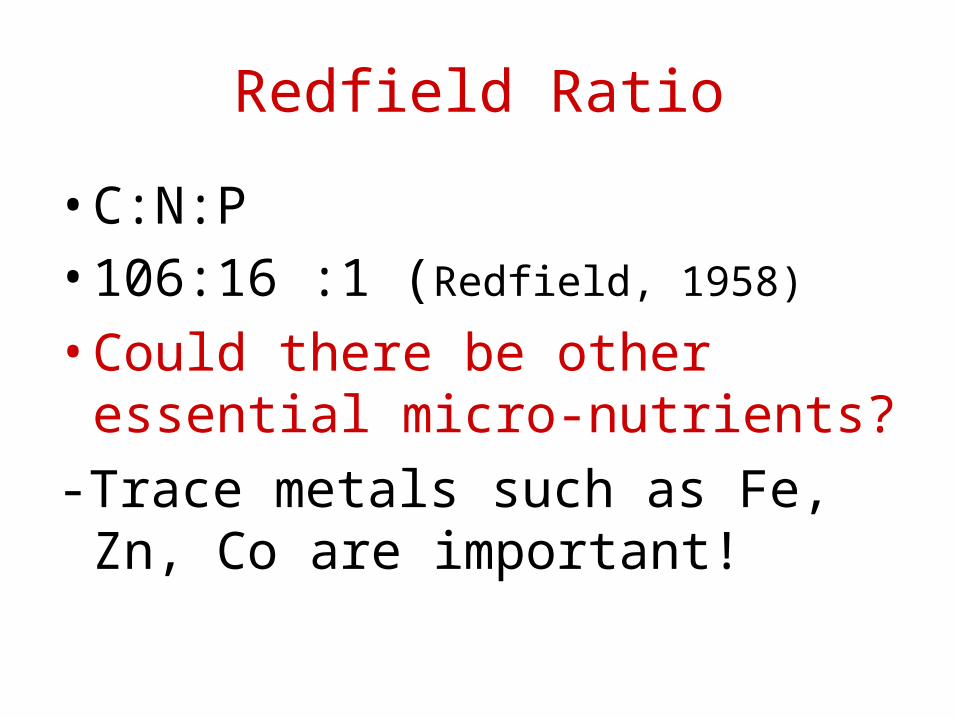
Redfield Ratio

• C:N:P• 106:16 :1 (Redfield, 1958)

• Could there be other essential micro-nutrients?

-Trace metals such as Fe, Zn, Co are important!

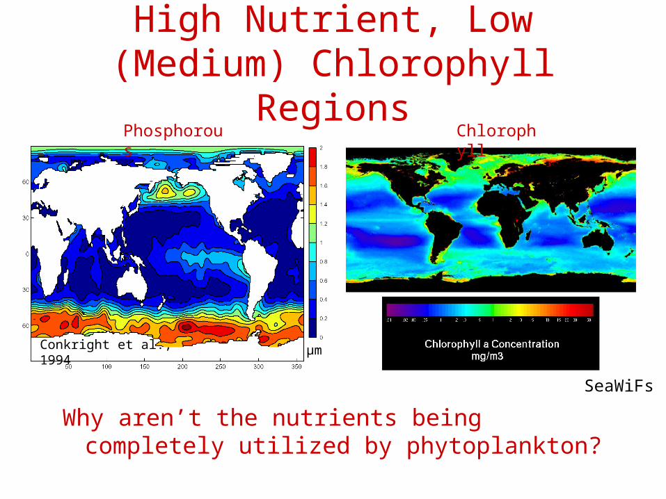
High Nutrient, Low (Medium) Chlorophyll Regions

Why aren’t the nutrients being completely utilized by phytoplankton?

Phosphorous Chlorophyll

Conkright et al., 1994 µm

SeaWiFs

Hypotheses

• Light

• Grazing

• Micronutrient limitation

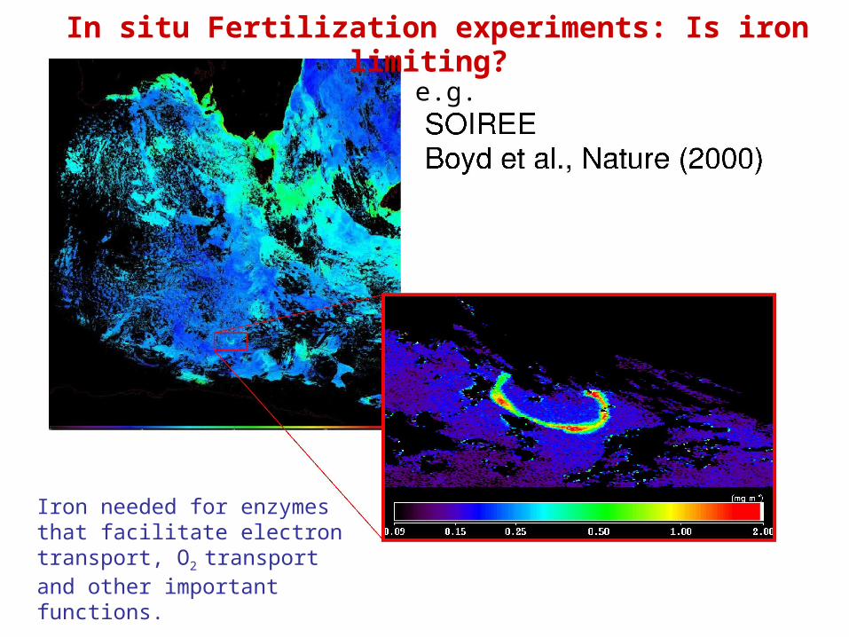
In situ Fertilization experiments: Is iron limiting?

e.g.

Iron needed for enzymes that facilitate electron transport, O2

transport and other important functions.

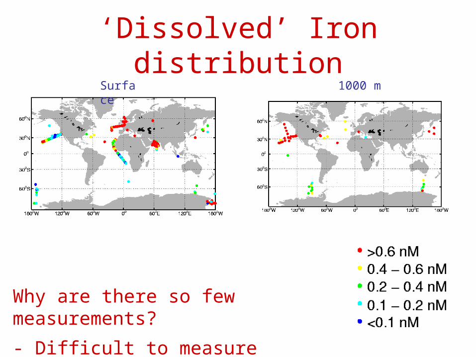
‘Dissolved’ Iron distribution

Why are there so few measurements?

- Difficult to measure

Surface 1000 m

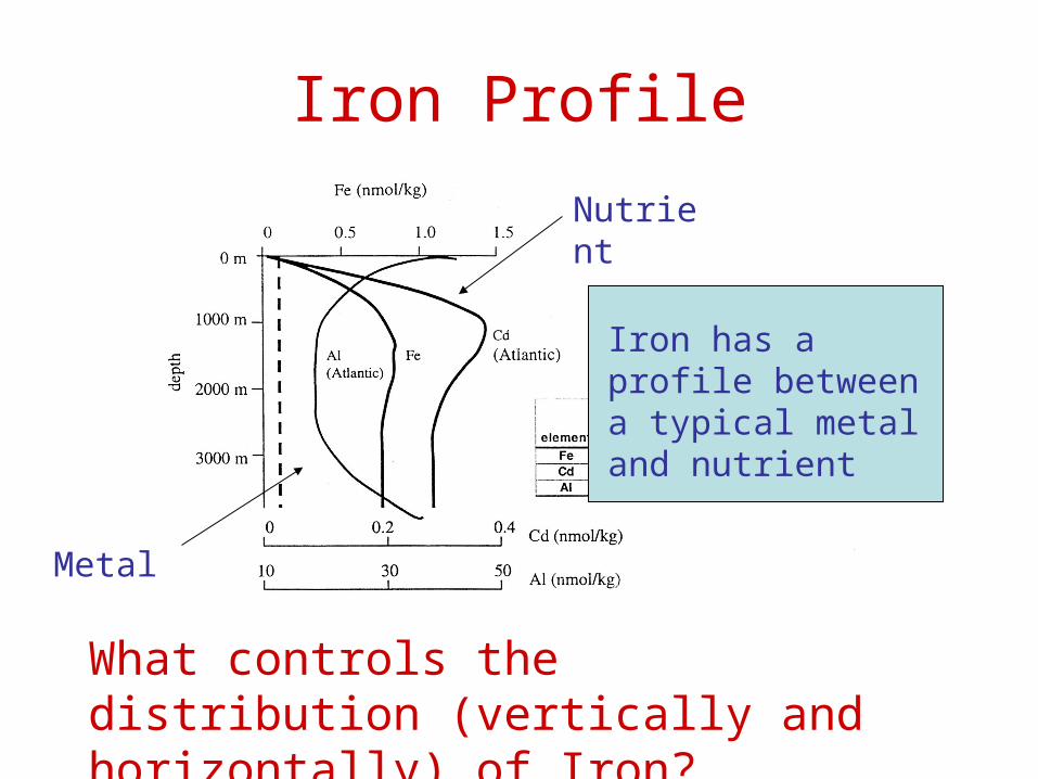
Iron Profile

What controls the distribution (vertically and horizontally) of Iron?

Iron has a profile between a typical metal and nutrient

Metal

Nutrient

Sources of Iron

• Riverine

• Continental Shelves

• Dust

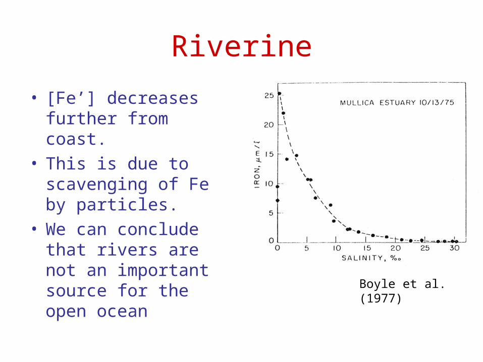
Riverine

• [Fe’] decreases further from coast.

• This is due to scavenging of Fe by particles.

• We can conclude that rivers are not an important source for the open ocean Boyle et al. (1977)

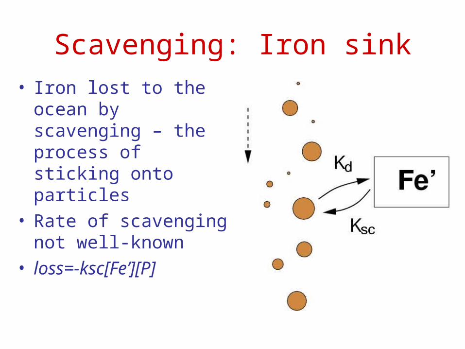
Scavenging: Iron sink• Iron lost to the ocean by

scavenging – the process of sticking onto particles

• Rate of scavenging not well-known

• loss=-ksc[Fe’][P]

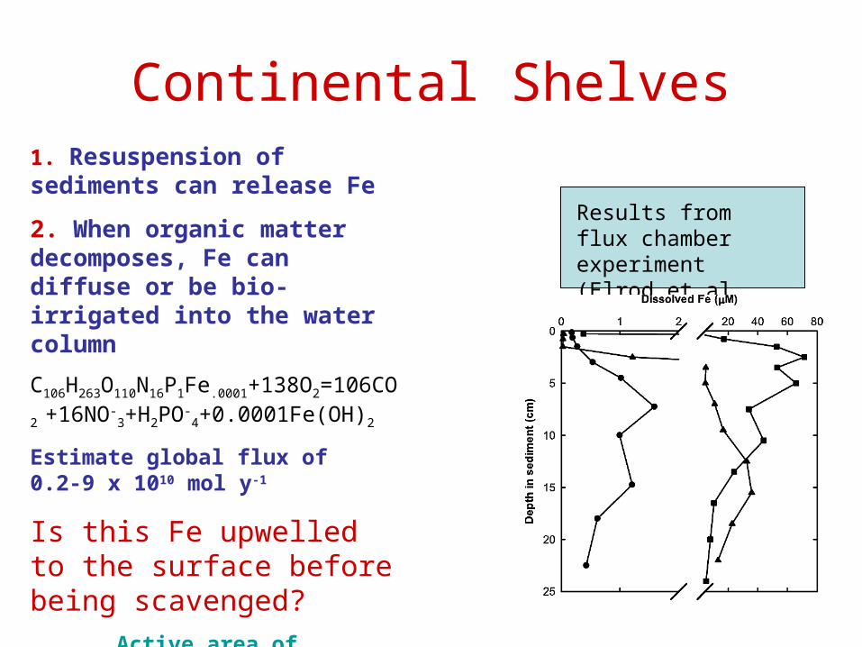
Continental Shelves1. Resuspension of sediments can release Fe

2. When organic matter decomposes, Fe can diffuse or be bio-irrigated into the water column

C106H263O110N16P1Fe.0001+138O2=106CO

2 +16NO-3+H2PO-

4+0.0001Fe(OH)2

Estimate global flux of 0.2-9 x 1010 mol y-1

Is this Fe upwelled to the surface before being scavenged?

Active area of research

Results from flux chamber experiment (Elrod et al., 2004)

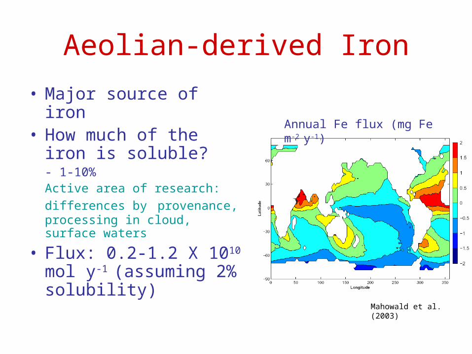
Aeolian-derived Iron

• Major source of iron• How much of the iron is

soluble?- 1-10%Active area of research:

differences by provenance, processing in cloud, surface waters

• Flux: 0.2-1.2 X 1010 mol y-1 (assuming 2% solubility)

Annual Fe flux (mg Fe m-2 y-1)

Mahowald et al. (2003)

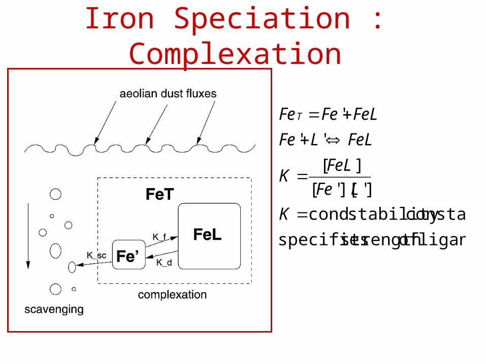
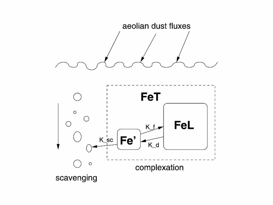
Iron Speciation : Complexation

ligand ofstrength specifies

constantstability cond.

]']['[

][

''

'

K

LFe

FeLK

FeLLFe

FeLFeFeT

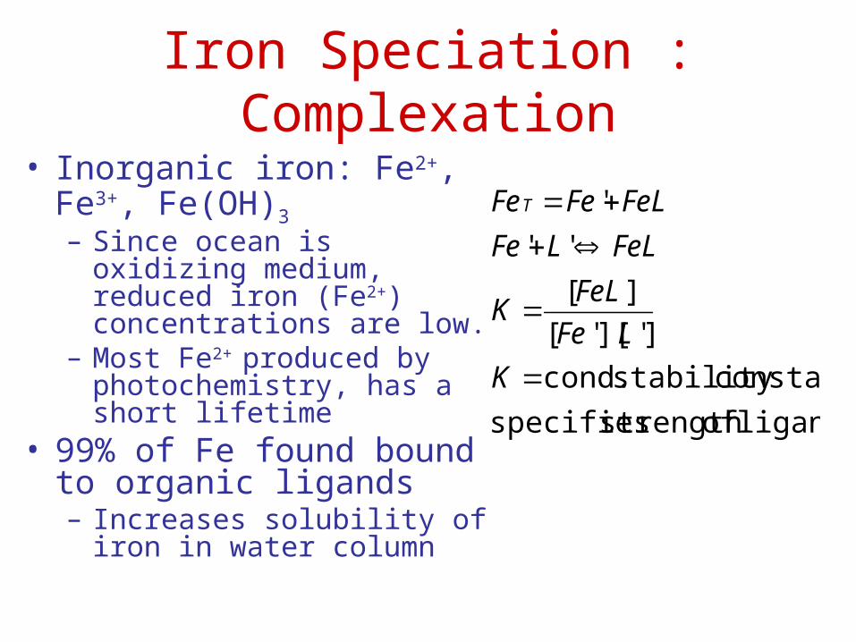
Iron Speciation : Complexation

• Inorganic iron: Fe2+, Fe3+, Fe(OH)3– Since ocean is oxidizing

medium, reduced iron (Fe2+) concentrations are low.

– Most Fe2+ produced by photochemistry, has a short lifetime

• 99% of Fe found bound to organic ligands– Increases solubility of iron in

water column

ligand ofstrength specifies

constantstability cond.

]']['[

][

''

'

K

LFe

FeLK

FeLLFe

FeLFeFeT

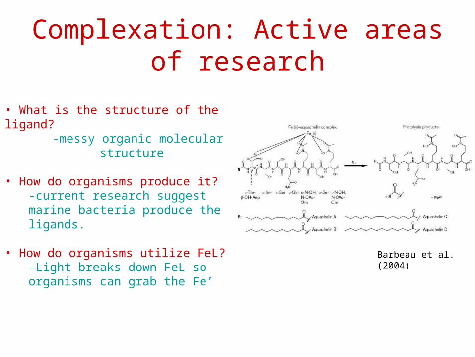
Complexation: Active areas of research

• What is the structure of the ligand?-messy organic molecular structure

• How do organisms produce it?-current research suggest marine bacteria produce the ligands.

• How do organisms utilize FeL?-Light breaks down FeL so organisms can grab the Fe’ Barbeau et al. (2004)

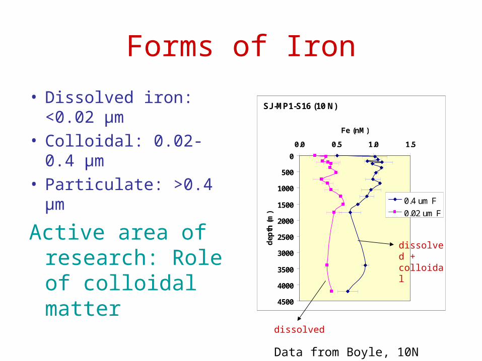
Forms of Iron

• Dissolved iron: <0.02 µm

• Colloidal: 0.02-0.4 µm• Particulate: >0.4 µm

Active area of research: Role of colloidal matter

SJ -MP1-S16 (10 N)

0

500

1000

1500

2000

2500

3000

3500

4000

4500

0.0 0.5 1.0 1.5

Fe (nM)

dep

th (m

)

0.4 um F

0.02 um F

Data from Boyle, 10N (Atlantic)

dissolved + colloidal

dissolved

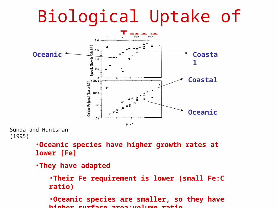
Biological Uptake of Iron

Oceanic

Coastal

•Oceanic species have higher growth rates at lower [Fe]

•They have adapted

•Their Fe requirement is lower (small Fe:C ratio)

•Oceanic species are smaller, so they have higher surface area:volume ratio

CoastalOceanic

Sunda and Huntsman (1995)Fe’

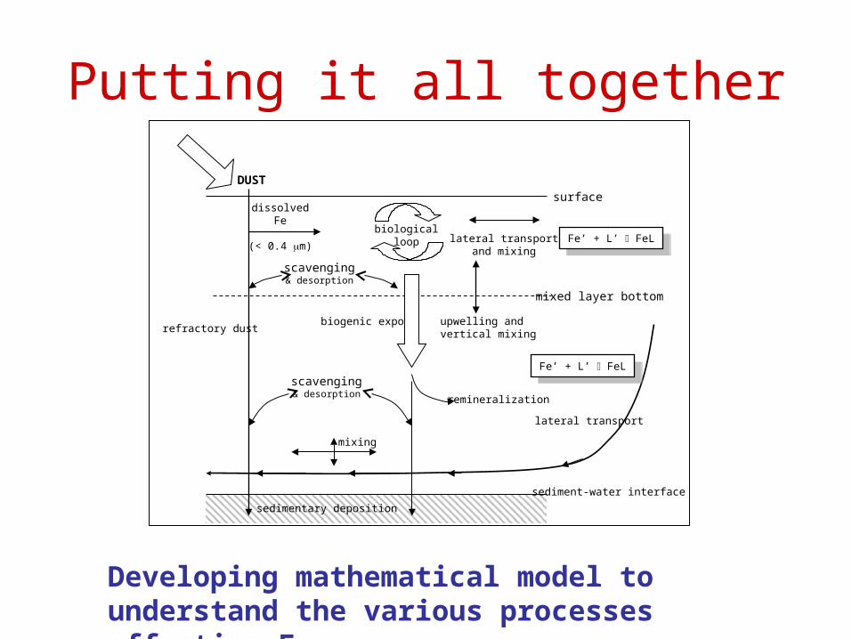
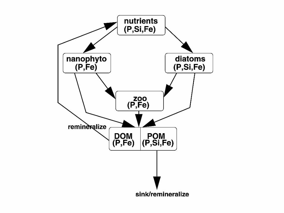
Putting it all together

biologicalloop

dissolvedFe

(< 0.4 m)

biogenic export

lateral transportand mixing

DUST

refractory dustupwelling andvertical mixing

mixed layer bottom

surface

remineralization

sediment-water interface

lateral transport

scavenging& desorption

mixing

sedimentary deposition

scavenging& desorption

Fe’ + L’ FeLFe’ + L’ FeL

Fe’ + L’ FeLFe’ + L’ FeL

Developing mathematical model to understand the various processes affecting Fe

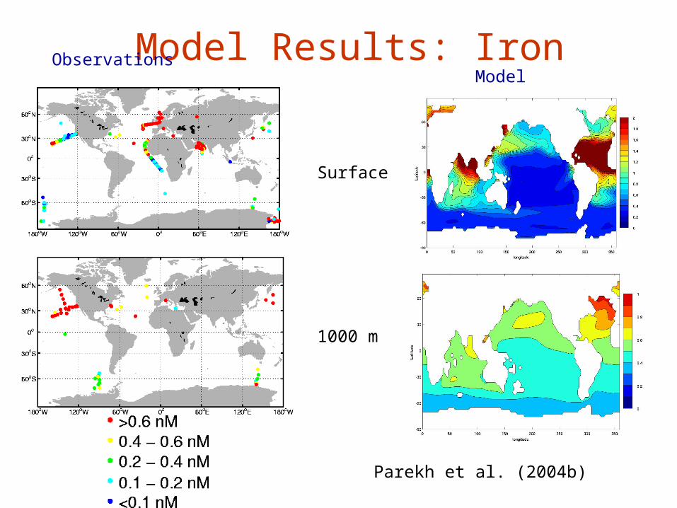
Model Results: Iron

Surface

1000 m

ObservationsModel

Parekh et al. (2004b)

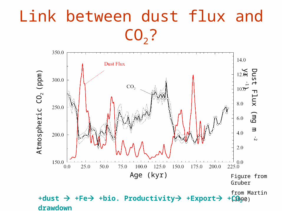
Link between dust flux and CO2?

Age (kyr)

Dust F

lux (mg m

-2 yr -1)

Atm

osph

eric

CO

2 (p

pm)

Figure from Gruber

from Martin (1990)

+dust +Fe +bio. Productivity +Export +CO2 drawdown

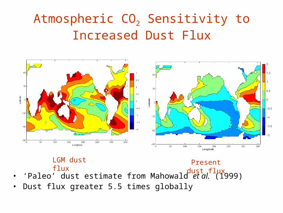
Atmospheric CO2 Sensitivity to Increased Dust Flux

• ‘Paleo’ dust estimate from Mahowald et al. (1999)• Dust flux greater 5.5 times globally

LGM dust flux Present dust flux

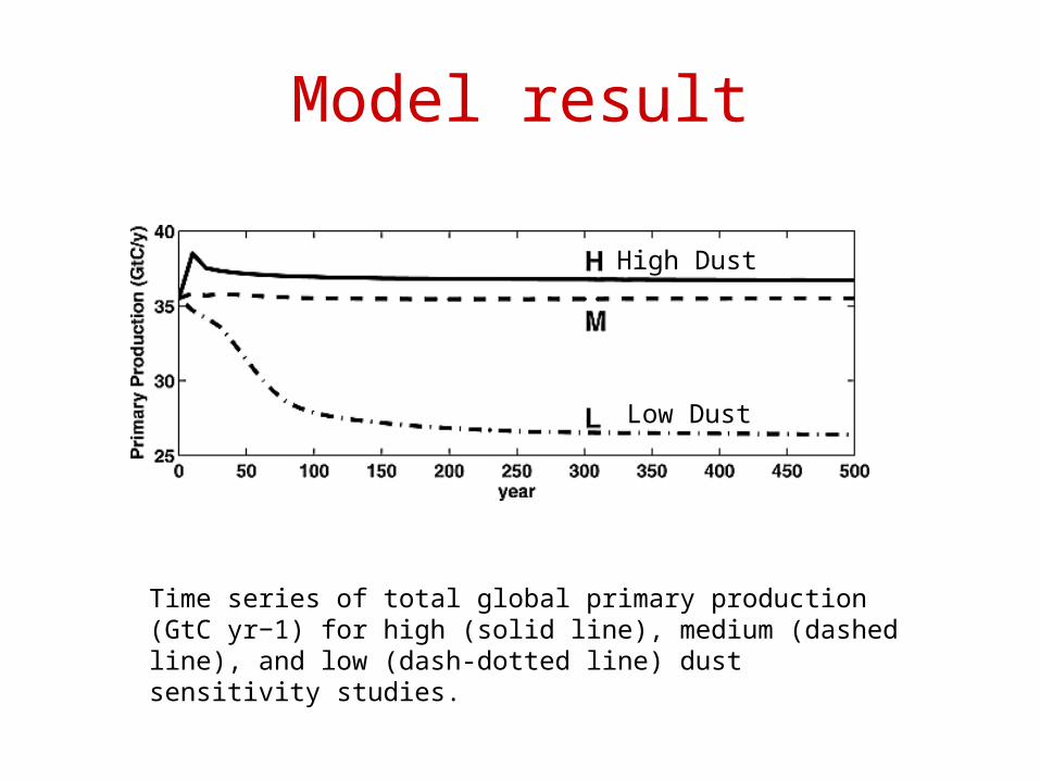
Time series of total global primary production (GtC yr−1) for high (solid line), medium (dashed line), and low (dash-dotted line) dust sensitivity studies.

Model result

High Dust

Low Dust

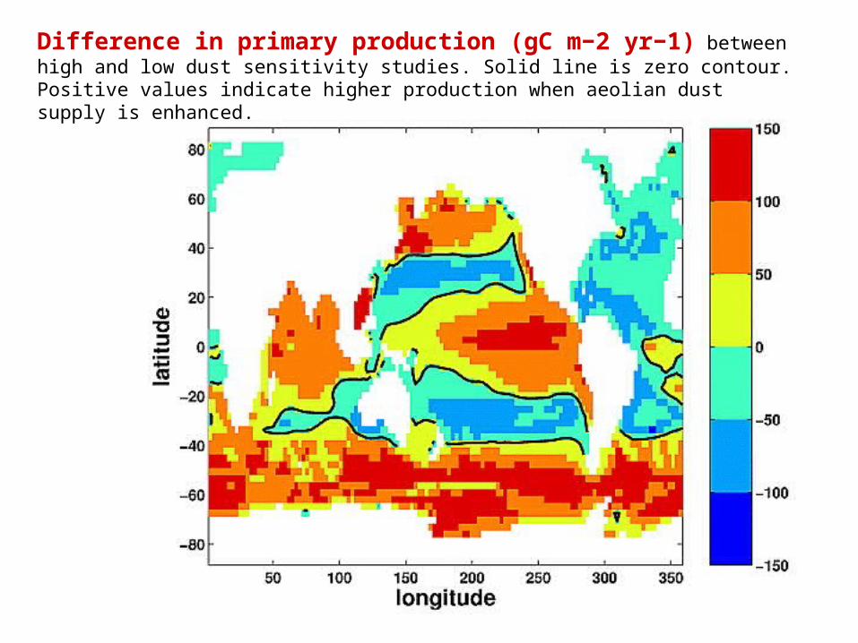
Difference in primary production (gC m−2 yr−1) between high and low dust sensitivity studies. Solid line is zero contour. Positive values indicate higher production when aeolian dust supply is enhanced.

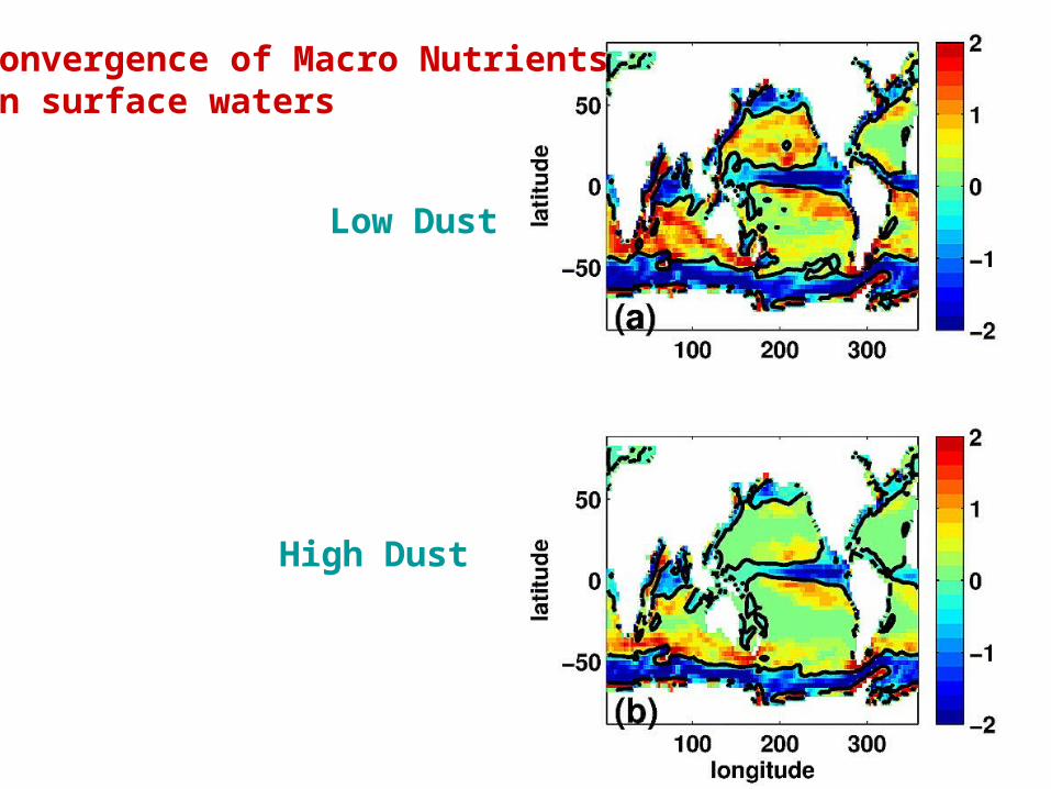
Low Dust

High Dust

Convergence of Macro Nutrients in surface waters

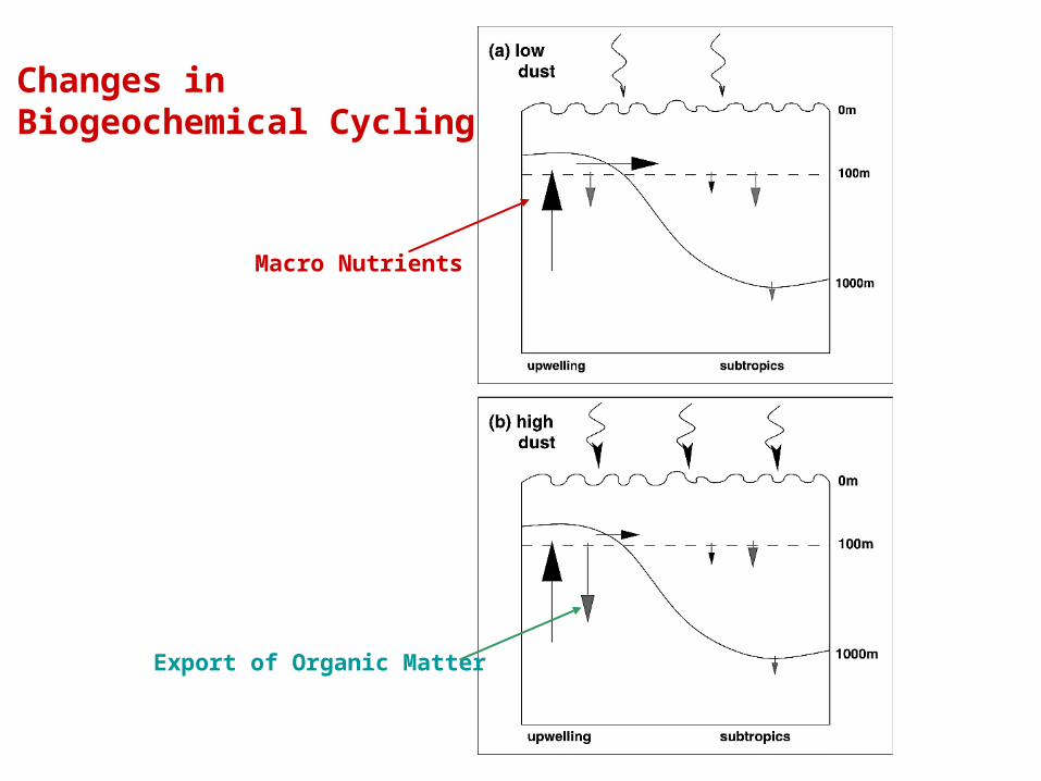
Macro Nutrients

Export of Organic Matter

Changes in Biogeochemical Cycling

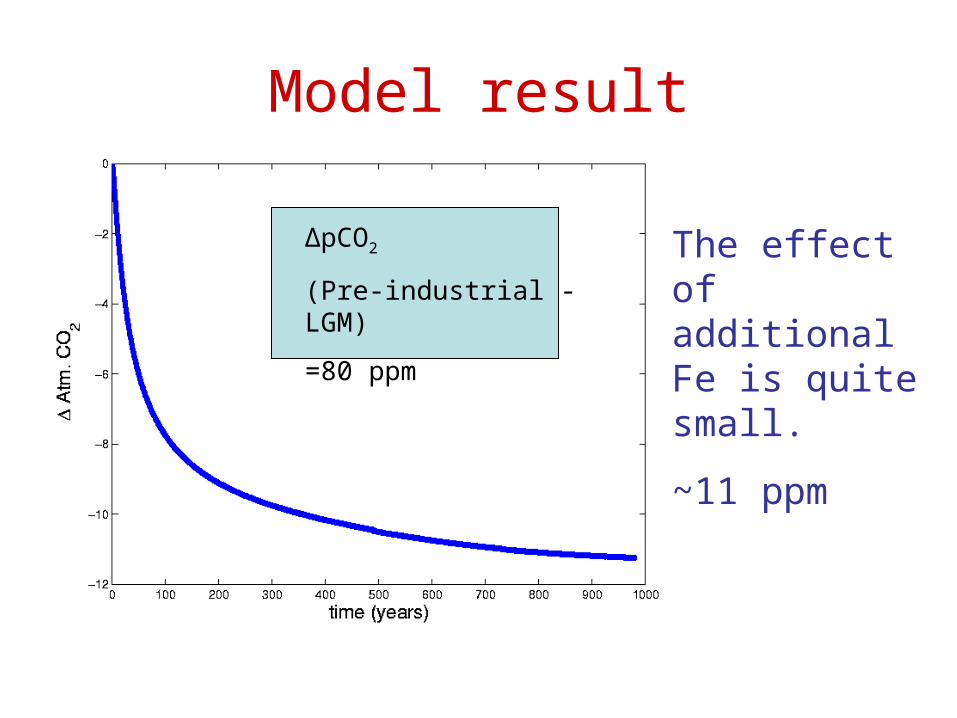
Model result

The effect of additional Fe is quite small.

~11 ppm

ΔpCO2

(Pre-industrial -LGM)

=80 ppm

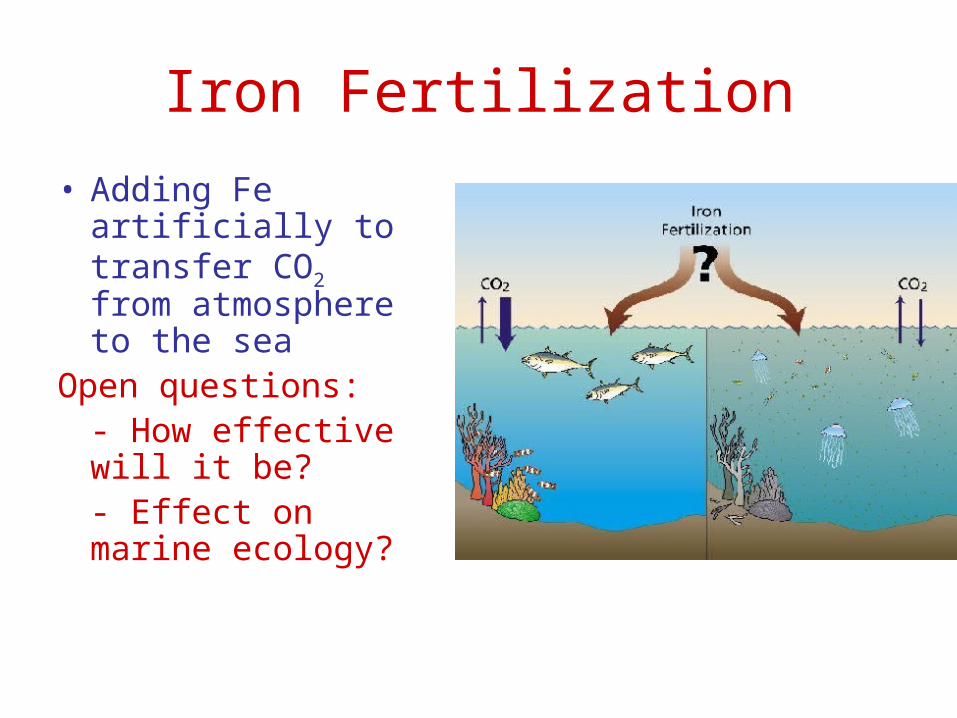
Iron Fertilization

• Adding Fe artificially to transfer CO2 from atmosphere to the sea

Open questions:- How effective will it be?- Effect on marine ecology?

End

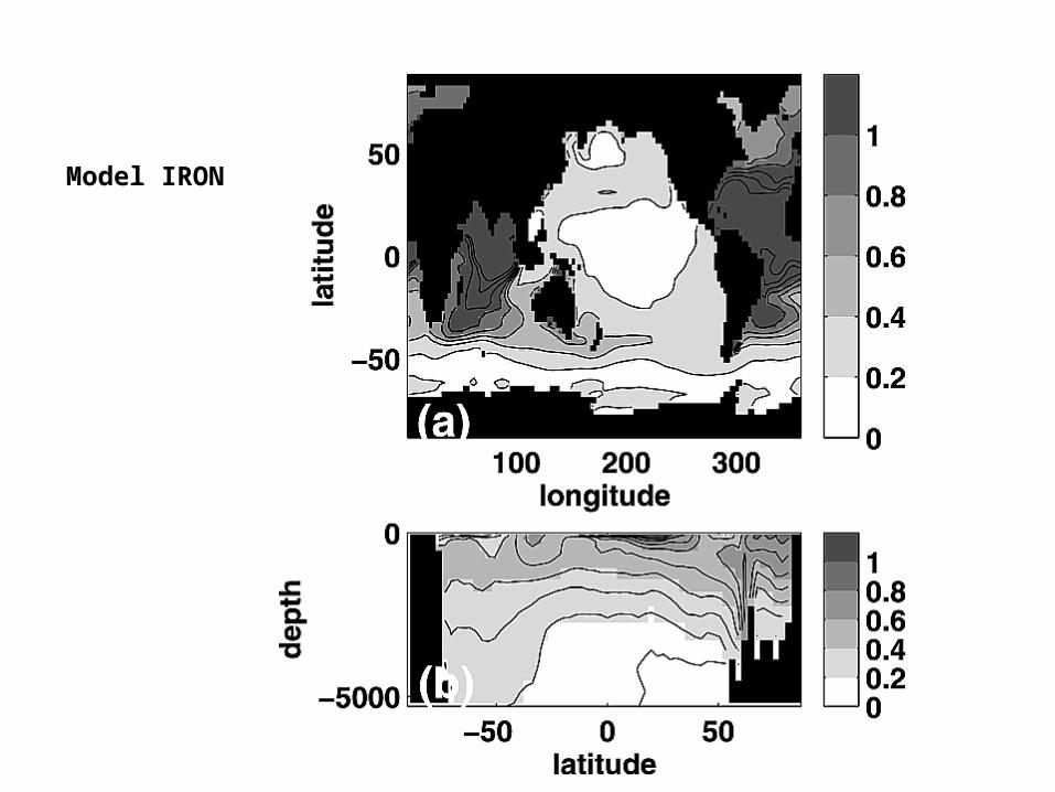
Model IRON