Louisiana State UniversityLSU Digital Commons

LSU Master's Theses Graduate School

2014

Iron Removal Using Electro- coagulation FollowedBy Floating Bead Bed FiltrationAsmita Anil PhadkeLouisiana State University and Agricultural and Mechanical College

Follow this and additional works at: https://digitalcommons.lsu.edu/gradschool_theses

Part of the Civil and Environmental Engineering Commons

This Thesis is brought to you for free and open access by the Graduate School at LSU Digital Commons. It has been accepted for inclusion in LSUMaster's Theses by an authorized graduate school editor of LSU Digital Commons. For more information, please contact gradetd@lsu.edu.

Recommended CitationPhadke, Asmita Anil, "Iron Removal Using Electro- coagulation Followed By Floating Bead Bed Filtration" (2014). LSU Master'sTheses. 1256.https://digitalcommons.lsu.edu/gradschool_theses/1256

IRON REMOVAL USING ELECTRO- COAGULATION FOLLOWED BY FLOATING BEAD BED FILTRATION

A Thesis

Submitted to the Graduate Faculty of the Louisiana State University and

Agricultural and Mechanical College in partial fulfillment of the

requirements for the degree of Master of Science

in

The Department of Civil and Environmental Engineering

by Asmita Phadke

B.E. Civil Engineering Government Engineering College, Aurangabad, Maharashtra, 2010

December 2014

ii

ACKNOWLEDGEMENTS

My sincere gratitude to my adviser, Dr. Malone, who gave me the opportunity of working

under his guidance. His support, motivation and channeling my thought process made me

accomplish all the positive results. I also thank him for having grandfatherly patience by listing

to all thousand pointless things I had to say. I thank Dr. Pardue and Dr. Theegala for being on my

committee and helping me through various problems I came across in working towards the

completion of this thesis. I thank God who makes all things possible and I thank him for giving

me the best adviser I could ever ask for. I thank my parents and my brother for their constant

support and care.

I thank Dr. Oetting for providing me financial support by letting me work as the

computer administrator for her lab. I also thank Dr. Wing who guided me at many stages in my

research work. I thank Dr. Blouin and Dr. Ying for helping me in statistics and SEM analysis

respectively. I am thankful to Mrs. Sandra Malone. I thank Ms. Cheryl, Mr. Robertson and my

friends Matthew, Daniel, Saoli, Jonathan, Marlon and Fatima for being of great help in

completing this project. Special thanks to Sima for having the setup ready for my experiments. I

also thank all my friends and family in the States.

iii

TABLE OF CONTENTS

ACKNOWLEDGEMENTS ............................................................................................................ ii

LIST OF TABLES ...........................................................................................................................v

LIST OF FIGURES ....................................................................................................................... vi

ABSTRACT ................................................................................................................................. viii

CHAPTER 1: INTRODUCTION ....................................................................................................1 1.1 Introduction ............................................................................................................................1 1.2 Research objectives ...............................................................................................................2 1.3 Organization of thesis .............................................................................................................3

CHAPTER 2: BACKGROUND .....................................................................................................4 2.1 Iron in Louisiana’s waters .....................................................................................................4 2.2 Iron standards and problems with presence of high iron concentrations ..............................5 2.3 Iron oxidation .........................................................................................................................6 2.4 Iron Removal Methodologies .................................................................................................7 2.5 Electrocoagulation and subsequent filtration of iron ..........................................................10 2.6 Adsorption- Oxidation iron removal method ......................................................................16

CHAPTER 3: PRELIMINARY STUIDIES .................................................................................20 3.1 Introduction .........................................................................................................................20 3.2 Materials and methods ........................................................................................................20 3.3 Results and discussion .........................................................................................................27 3.4 Conclusions .........................................................................................................................32

CHAPTER 4: IRON REMOVAL EFFECIENCY OF A FLOATING BEAD BED BY APPLICATION OF ELECTROCOAGULATION ......................................................................34

4.1 Introduction .........................................................................................................................34 4.2 Background .........................................................................................................................35 4.3 Materials and methods ........................................................................................................36

4.3.1 Iron removal at pH 8 .................................................................................................38 4.3.2 Iron removal at pH 6 .................................................................................................39

4.4 Results and discussion .........................................................................................................40 4.4.1 Iron removal at pH 8 .................................................................................................40 4.4.2 Iron removal at pH 6 .................................................................................................42 4.4.3 Comparison of removals obtained at pH 8 and 6 ......................................................45

4.5 Conclusions ..........................................................................................................................46

CHAPTER 5: IRON REMOVAL EFFICIENCY OF IRON PRECOATED FLOATING BEAD BED BY APPLICATION OF ELECTROCOAGULATION ........................................................48 5.1 Introduction .........................................................................................................................48 5.2 Background .........................................................................................................................49

iv

5.3 Materials and methods ........................................................................................................49 5.3.1 Experimental coating ................................................................................................49 5.3.2 Iron removal efficiency of iron precoated floating beads using electrocoagulation .51

5.4 Results and discussion .........................................................................................................54 5.4.1 Experimental coating ...............................................................................................54 5.4.2 Iron removal efficiency of iron precoated floating beads using electrocoagulation .57

5.5 Conclusions .........................................................................................................................60

CHAPTER 6: CONCLUSIONS AND RECOMMENDATIONS .................................................61

REFERENCES ..............................................................................................................................65

APPENDIX A: STATISTICAL ANALYSIS ................................................................................68

APPENDIX B: DATA COLLECTED...........................................................................................72

VITA ..............................................................................................................................................81

v

LIST OF TABLES

Table 2.1 USGS survey between 1992-2003 detected high iron concentrations in Louisiana’s aquifer system (Ayotte et al., 2011) .................................................................................................4

Table 2.2: Rate of conversion of ferrous to ferric slows down dramatically on decreasing the pH (Vance, 1994) ..................................................................................................................................7

Table 2.3: Summary of different methods used for iron removal....................................................8

Table 2.4: Electrocoagulation process depicted almost 100% contaminant removal with system specific conditions ........................................................................................................................13

Table 2.5: Optimum conditions required for effective electrocoagulation ...................................14

Table 2.6: Factors influencing iron adsorption- oxidation technique gives a small range of pH over which the process is effective (Sharma, 2001) .....................................................................18

Table 3.1: Time required to generate specified amount of aluminum coagulant is inversely proportional to the amperes applied ..............................................................................................25

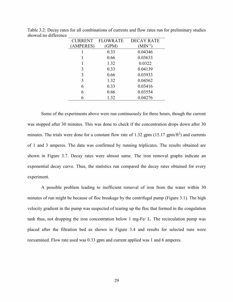
Table 3.2: Decay rates for all combinations of currents and flow rates run for preliminary studies showed no difference ....................................................................................................................29

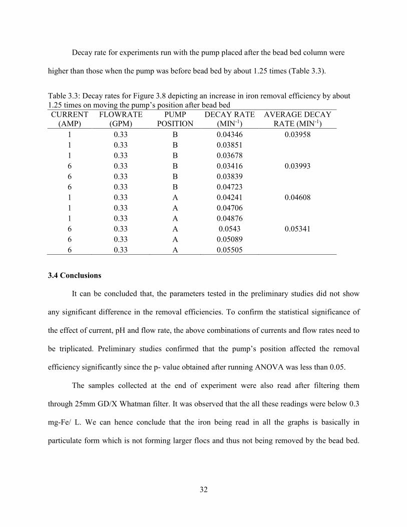
Table 3.3: Decay rates for Figure 3.8 depicting an increase in iron removal efficiency by about 1.25 times on moving the pump’s position after bead bed ...........................................................32 Table 4.1: Decay rates for data plotted in Figure 4.3 hardly differed from each other representing no distinguishing pattern ...............................................................................................................42

Table 4.2: Decay rates for iron removal at pH 6 (Figure 4.4) gave two to three times high removal at the lowest flowrate & lowest current compared to other combinations .....................44

Table 4.3: Distribution by weight of oxygen, aluminum and iron in water sample analyzed by SEM observed that enough aluminum was present for coagulation of iron. ................................45

Table 5.1: Decay rates for data plotted in Figure 5.6 show 3.5 times higher iron removal at 1 ampere current compared to 6 amperes when flow rate was 0.33 gpm ........................................58

Table 6.1: List of recommended optimum range of parameters for achieving high iron removal efficiency using electrocoagulation prior to bead filtration ..........................................................63

vi

LIST OF FIGURES

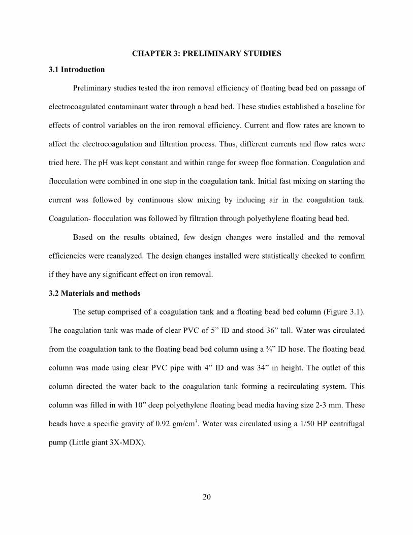
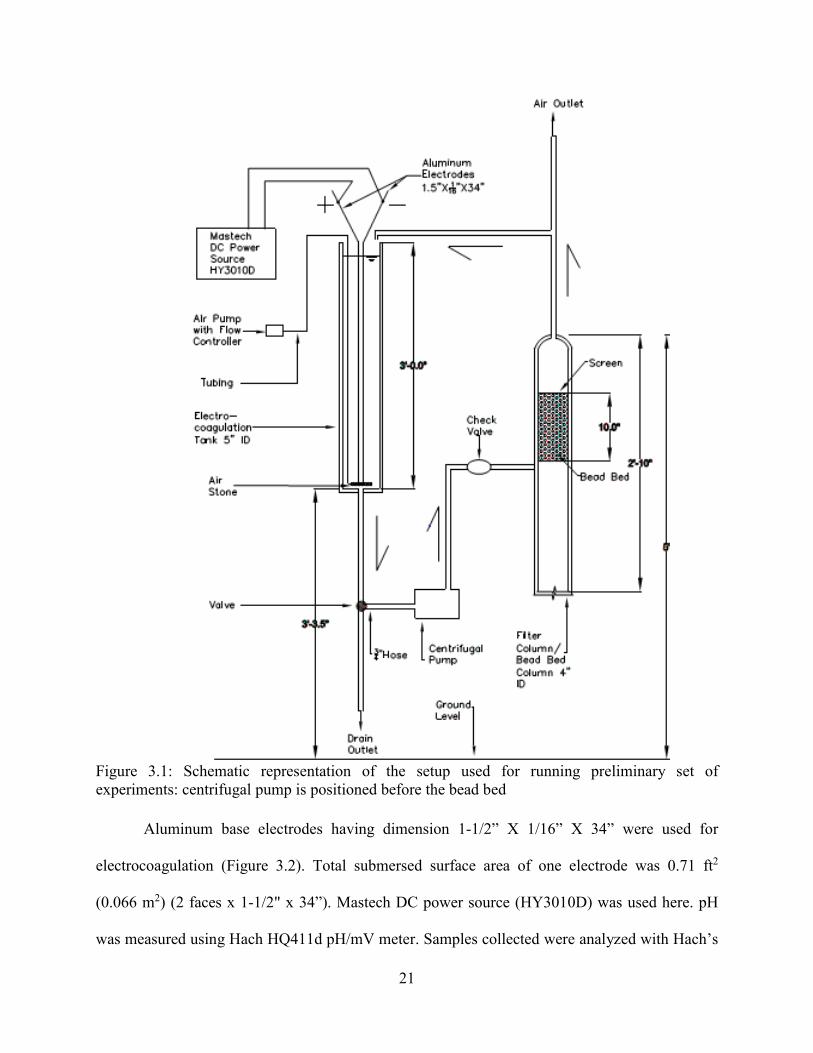
Figure 3.1: Schematic representation of the setup used for running preliminary set of experiments: centrifugal pump is positioned before the bead bed ................................................21

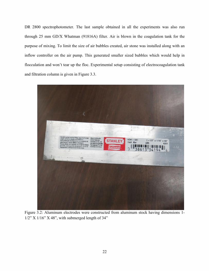
Figure 3.2: Aluminum electrodes were constructed from aluminum stock having dimensions 1-1/2” X 1/16” X 48”, with submerged length of 34” ......................................................................22

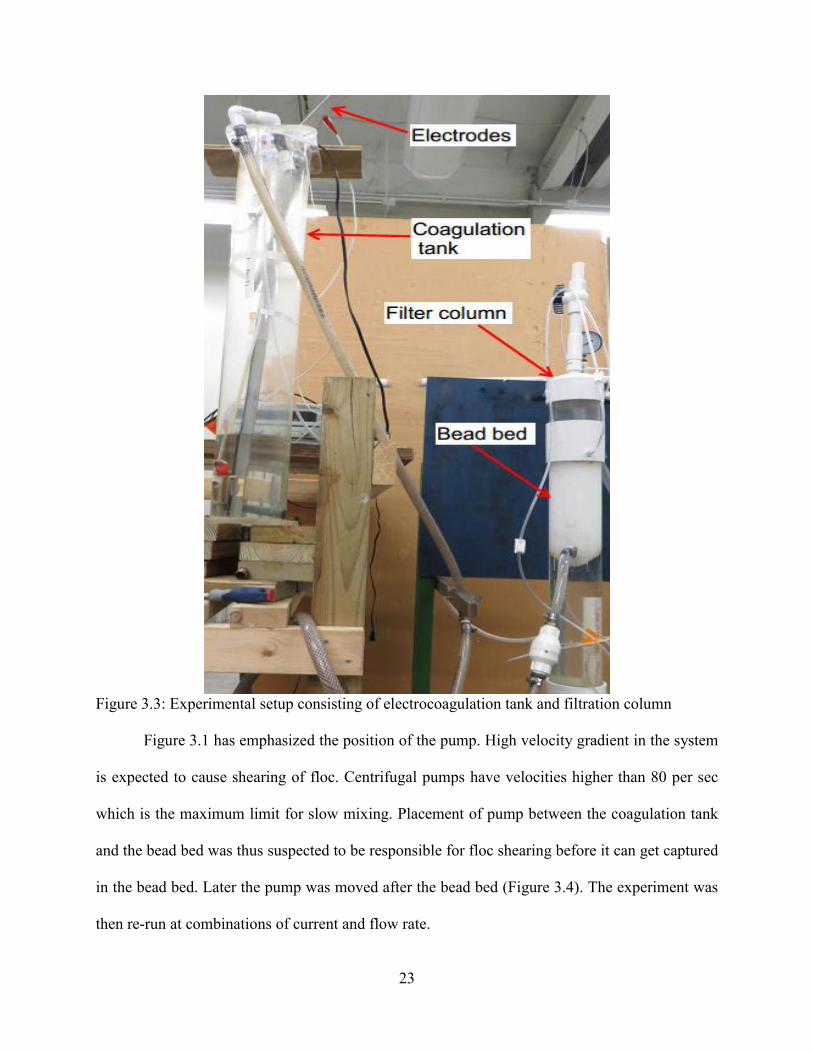
Figure 3.3: Experimental setup consisting of electrocoagulation tank and filtration column ......23

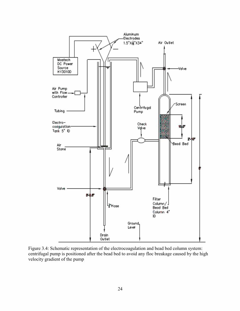
Figure 3.4: Schematic representation of the electrocoagulation and bead bed column system: centrifugal pump is positioned after the bead bed to avoid any floc breakage caused by the high velocity gradient of the pump ........................................................................................................24

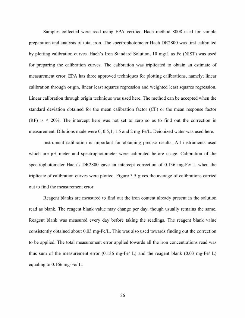
Figure 3.5: Average plot of three calibrations estimated the measurement error of 0.136 mg-Fe/ L for spectrophotometer Hach DR2800 ............................................................................................27

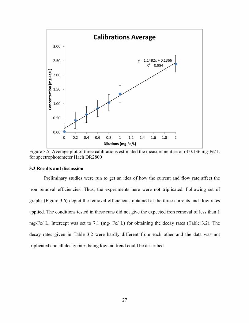
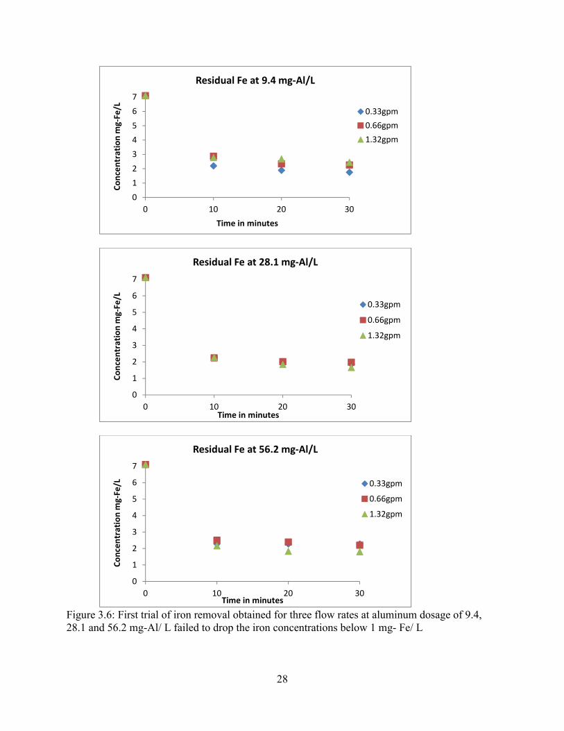
Figure 3.6: First trial of iron removal obtained for three flow rates at aluminum dosage of 9.4, 28.1 and 56.2 mg-Al/ L failed to drop the iron concentrations below 1 mg- Fe/ L ......................28

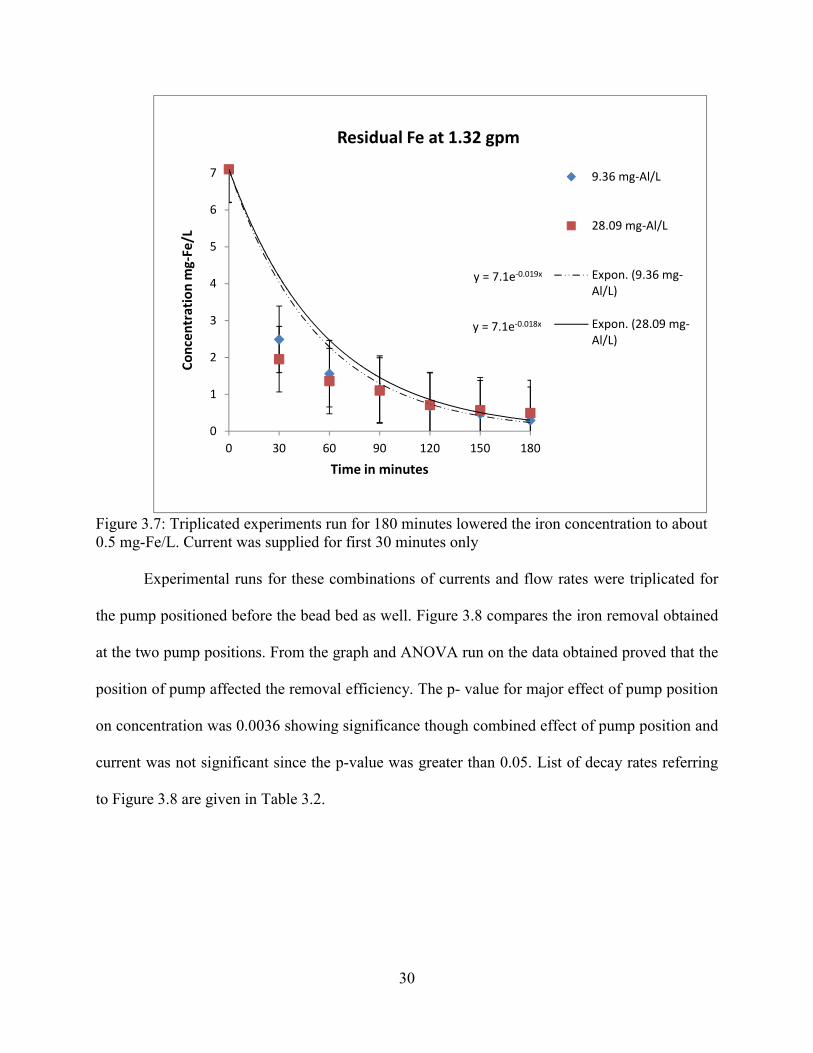
Figure 3.7: Triplicated experiments run for 180 minutes lowered the iron concentration to about 0.5 mg-Fe/L. Current was supplied for first 30 minutes only .......................................................30

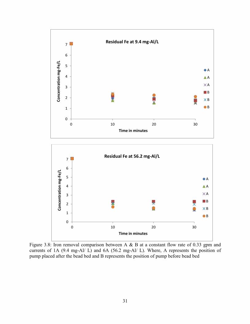
Figure 3.8: Iron removal comparison between A & B at a constant flow rate of 0.33 gpm and currents of 1A (9.4 mg-Al/ L) and 6A (56.2 mg-Al/ L). Where, A represents the position of pump placed after the bead bed and B represents the position of pump before bead bed ............31

Figure 4.1: Schematic representation of experimental setup consisting of coagulation tank and the filtration column .......................................................................................................................37

Figure 4.2: Fresh polyethylene floating beads sized 2-3 mm can capture solids as small as 50 microns ..........................................................................................................................................38

Figure 4.3: Iron concentrations did not drop below 1 mg-Fe/ L for any of the combinations of mg-Al/ L released in water and flow rates run at a pH of 8...........................................................41

Figure 4.4: Efficient iron removal obtained within first 10 minutes of run at pH 6 on applying 9.4 & 56.2 mg-Al/ L ...........................................................................................................................43

Figure 4.5: Scanned electron microscopic image of the effluent represented the caked particles formed after post- filtration process showed particulate residual .................................................44

Figure 4.6: The rate of iron removal was found to be significantly higher at a pH of 6 when compared to iron removals obtained at pH 8 .................................................................................46

Figure 5.1: Experimental setup for demonstrating adsorption- oxidation mechanism successfully coated the polyethylene plastic beads ...........................................................................................50

vii

Figure 5.2: Schematic representation of electrocoagulation and filtration unit used for obtaining iron removal efficiencies of fresh beads and iron precoated beads ..............................................52

Figure 5.3: Experimental unit consisting of coagulation tank followed by precoated floating bead bed column. ...................................................................................................................................53

Figure 5.4: Visible iron coating on sand media was observed within a day as compared to polyethylene beads which took three days (a) Iron coated sand media and (b) Iron coated polyethylene bead media................................................................................................................55

Figure 5.5: Scanned electron microscopic images of beads at 100 and 10 µm showing formation of dense iron coating with increased surface roughness (a) Bead #1 and (b) Bead #2 ..................56

Figure 5.6: Plot of iron removals obtained at 9.4 and 56.2 mg-Al/ L by using precoated beads showed good removal at the lowest flow rate of 0.33 gpm ..........................................................57

Figure 5.7: Best removal obtained by using iron precoated beads at the lowest flowrate as compared to fresh beads (Each data point represents average of triplicates) ...............................59

Figure 6.1: Flow diagram for continuous system .........................................................................63

viii

ABSTRACT

High iron concentrations in the water used for aquaculture results in stock losses. It is

necessary to drop down the iron concentrations to levels which can be handled by the fish.

Electrocoagulation followed by floating bead bed filtration was used to remove iron from water.

Electrocoagulation was carried out using aluminum electrodes. The flocs formed in the

coagulation tank were then filtered out using 2-3 mm polyethylene floating beads having specific

gravity of 0.92 gm/cm3. Proper retention time of ≥ 10 min, pH of 6±0.2, Al3+ coagulant dosage

of about 9 mg-Al3+/ L and flow rate ≤ 0.4 gpm resulted in dropping down the iron concentrations

to 0.3 mg- Fe/ L within 10 minutes of run time.

Adsorption- oxidation mechanism is applied for forming iron coated media. Iron

precoated media can accelerate iron removal by improving adsorption due to increase in surface

area of media. The adsorption- oxidation mechanism was used to form iron coatings on the

polyethylene bead media. Iron accumulation ranging from 5.93 * 10-5 mg/ cm2 to 7.71* 10-5 mg/

cm2 was observed at the end of three days. The iron precoated beads were later checked for their

iron removal efficiency by prior application of electrocoagulation. The iron removal efficiencies

of fresh beads vs iron precoated beads were then compared. Iron precoated beads proved better

than fresh beads with 3.5 times increase in its iron removal efficiency. Polyethylene beads used,

lacked a negative surface compared to sand media and required a longer time for coat formation.

Iron removal by application of adsorption- oxidation method may be used at places where time

of treatment is not the constraint.

1

CHAPTER 1: INTRODUCTION

1.1 Introduction

Iron is one of the most abundant resources comprising 0.5 to 5% of earth’s crust (Ityel,

2011; Vance, 1994). High iron concentrations in water give them a reddish color in the presence

of oxygen and are responsible for problems like staining, taste issues, stock losses in aquaculture

and pipe fouling. Environmental protection agency (EPA) identifies iron as a secondary

contaminant since it is not considered as a health hazard to humans. Secondary maximum

contaminant level set by EPA for amount of total iron in public water systems is 0.3 mg- Fe/L

(EPA, 2013).

The aquaculture industry requires high quality water to rear fish for food, display and

conservation purposes. The permissible water contaminant levels for aquaculture can be lower

than those set for drinking water. For iron, the contaminant of concern here, permissible limit of

total iron present in aquaculture waters range from 0.15 mg- Fe/L to 0.5 mg- Fe/L (warm water)

(Conte, 1993). Groundwater containing high quantity of total iron is harmful for the survival of

fish. Iron can be present in ferrous or ferric form depending on the pH of water. Low redox

reflecting the absence of oxygen favors the formation of ferrous iron from iron minerals

contained in soils. Ferrous or ferric ions are released from minerals based on their solubility

constants. Southern Louisiana groundwater has a lower pH due to CO2 (H2CO3) accumulation

from organic decay processes, favoring high Fe2+ concentrations. Iron present needs to be

removed prior to use in aquaculture systems.

Water purification systems employ various treatment methods for iron removal like water

softening, ion exchange, ozonation and media filtration. In recent years, electrocoagulation has

been depicted as an effective technique for the removal of chromium, iron, copper, zinc, lead and

2

manganese, with removal efficiencies ranging between 90- 100% (Ghosh et al., 2008; Kongjao et

al., 2008; Orescanin et al., 2011; Petsriprasit et al., 2010). The removal efficiencies depend on

system conditions like pH, current, electrolysis time, size of electrodes, type of electrode used,

coagulant dosage, velocity gradient and flux rate.

Another method of iron removal is adsorption- oxidation. This technique can be

employed to remove ferrous iron from water. Ferrous iron gets adsorbed to the media surface

followed by its oxidation to ferric iron. Adsorption may occur due to Van der Waals forces or by

chemical bonds. Low amount of oxygen and pH favors the presence of ferrous than ferric iron.

Thus, for adsorption to occur the system pH needs to be between 6 - 6.5 and environment must

be oxygen free. Once adsorption is complete, oxidation of ferrous to ferric is enforced. This

results in formation of an iron coat around the media. This process has been well demonstrated

for sand media by Sharma, 2001. Similar method and conditions were used to generate iron

coating on bead media.

1.2 Research objectives

The objectives of this research were as follows:

1) Determine if an aluminum based electrocoagulation process will enhance the iron

removal capabilities of a floating bead bed.

2) Verify the mechanism causing iron adhesion to floating beads

3) Determine if bead coating enhances iron removal efficiency.

4) Establish operational conditions for floating bead beds used for iron removal.

The hypotheses of this research were:

1) Higher current amounts will help in increasing the iron removal efficiency.

2) High iron removal efficiency would be obtained with iron precoated beads.

3

1.3 Organization of thesis

Chapter II of thesis describes the background information on factors controlling iron

removal. Chapter III includes the preliminary study carried out for testing the effect of different

currents in electrocoagulation and varying flow rates on the iron removal efficiency of floating

bead bed. Based on results obtained from the preliminary study, a few changes in the design of

apparatus were made and the experiments were re-run. These results are described in chapter III.

Chapter IV includes triplicates of experiments run in chapter III. Experiments run at 0.33, 0.66

and 1.32 gpm were triplicated. Currents applied here were 1, 3 and 6 amperes. Chapter V

includes the formation of iron precoated beads using adsorption- oxidation technique. Iron

removal efficiency of the precoated beads was also tested at similar conditions as carried out in

experimental runs in chapter IV. Graphs of iron concentration vs. time were plotted. Difference

in the iron removal efficiencies was then compared in chapter V.

4

CHAPTER 2: BACKGROUND

2.1 Iron in Louisiana’s waters

Iron is one the most common element found in the earth’s crust. This metal has an atomic

number 26. Iron usually can be found in ores along with other elements. Dissolved iron mostly

exists in ferrous (Fe2+) or ferric (Fe3+) oxidation states. The soluble ferrous iron form is dominant

in anaerobic environments. In the presence of oxygen, both ionic iron forms would convert to

iron hydroxide, eventually precipitating out from water. About 1.3 X 10-3 mg/ L of iron is

dissolved in ocean waters (Silver, 1993). USGS scanned the presence of trace elements in

groundwater across United States from 1992- 2003 (Ayotte et al., 2011). This report has

identified Louisiana’s climatic conditions and other parameters like pH, redox, aquifer type and

iron concentration from samples collected from various aquifers. The data reported is

summarized in Table 2.1.

Table 2.1 USGS survey between 1992-2003 detected high iron concentrations in Louisiana’s aquifer system (Ayotte et al., 2011)

PARAMETER RANGE/ CONDITION Climatic condition ≈ 85% Humid pH of precipitation 4.2 to 5.0

Redox Anoxic, oxic as well as mixed conditions Aquifer rock type Semiconsolidated sand aquifers Iron concentration > 0.3 mg- Fe/ L

Louisiana’s aquifer system have been described as coastal lowland aquifer system formed

of semiconsolidated sand, silt, clay and few percent of carbonate rocks. The water samples

scanned by USGS depicted a mixture of oxic and anoxic environment. Most groundwater in a

humid region has anoxic conditions. Iron concentrations detected in Louisiana’s aquifers were

mostly greater than 0.3 mg- Fe/ L. Some, aquifers however displayed a lower iron concentration

ranging between 0.001 to 0.3 mg- Fe/ L (Ayotte et al., 2011). The U.S. Geological Survey

5

(USGS) and the Louisiana Department of Environmental Quality (LDEQ) studied the 1700 mile

stretch of the Mississippi river and found that many alluvial aquifers in Louisiana have high iron

contents. While, the Cockfield and Sprata aquifers in Louisiana had iron contents just above 0.3

mg/L, some samples analyzed from alluvial aquifer group had iron amounts between 50 to 100

mg/L (National Water Summary, 1986).

Almost half of Louisiana’s population uses the groundwater as its drinking water source.

Louisiana’s humid climate, anoxic groundwater supported by lower pH supports the presence of

high ferrous iron concentrations in groundwater. The incentive of doing this project came from

the fact that the Mississippi river, its tributaries and ground water present in Louisiana contains

high amount of ferrous iron. This is limiting its use in aquaculture industry. These high iron

concentrations caused a bead filter tested in New Roads near the Mississippi River to fail. The

iron got coated around the beads which made them sink.

2.2 Iron standards and problems with presence of high iron concentrations

Permissible limit for iron in drinking water has been reported as low as 0.2 mg- Fe/ L

(Tekerlekopoulou 74, EC-Official Journal of the European Communities Council Directive).

World Health Organization (WHO) has set the secondary contaminant level for iron at 0.3 mg-

Fe/ L. Iron is considered as a secondary contaminant since it is not harmful for human beings but

causes other problems like staining, taste and color issues. Iron concentration as low as 0.3 mg/L

can give waters reddish brown color. Presence of higher contents of iron in the form of iron

hydroxide or ferrous bicarbonate in domestic water supply can cause blockages in pipes

(Chaturvedi, 2012). The reactive nature of iron can cause severe problems in groundwater

remediation systems. The anaerobic groundwater conditions reduce the ferric to ferrous iron

which is then hard to extract due to its high solubility.

6

Higher iron contents though not harmful to human beings but can result in loss of fish.

Aquaculture raises the fish in high quality water and under controlled environments. Poor water

quality can have drastic effects on the stock. Dissolved oxygen, alkalinity, salinity, pH, hardness,

contaminant levels all affect the health of stock. Recirculating aquaculture systems have water

recirculating through the system thus, reusing the water. Timely cleaning of water used for

aquaculture is often necessary, to maintain healthy and optimum environmental conditions for

the stock. Tolerance level for iron concentration in aquaculture for salmonid quality standard has

been given as 0.00 to 0.15 mg-Fe/ L and up to 0.5 mg-Fe/L for warm water situations (Conte,

1993). Most fish cultures cannot handle iron stress above 0.5 mg/L (Buttner et al., 1993). Kenny

et al., (2009) surveyed that aquaculture industry in Louisiana accounts for 3% of total

groundwater usage.

2.3 Iron oxidation

Oxidation states of iron can range from –II to +VI. Out of these, only +II ferrous and +III

ferric states are common. Lower oxides of iron, ranging from –II to I are seen as carbonyls,

nitrosyls, phosphines and its derivatives. Presence of excess carbonate (CO32-) in groundwater

and exposure to air will cause the conversion of ferrous to FeCO3, leading to formation of brown

deposits of ferric oxide (Silver, 1993). Ferrous in its pure form in water can result in a light

turquoise color reflecting the presence of hexaquo ferrous ion [Fe(H2O)6]2+. Oxidation of 1 mg

of ferrous iron to ferric requires about 0.14 mg of oxygen (Sharma, 2001).

The amount of iron present or removed depends on a variety of parameters including pH,

temperature, dissolved oxygen level, oxidation state and the presence of other soluble ions.

Temperature, pH and dissolved oxygen content have an inverse relation with the rate of

oxidation. An example given by Vance, 1994 gives the time and pH required for 90% oxidation

7

of ferrous iron at 21°C with critical dissolved oxygen concentration of 2 mg/L (Table 2.2).

Harmon, 2003 also supports that at pH greater than 6.5 promotes rapid conversion of ferrous iron

to ferric iron. Stumm and Lee, 1961 report that the rate of oxygenation of ferrous iron increases

100 folds per unit increase in pH. Fe(OH)3 is one of the predominate iron species that can be

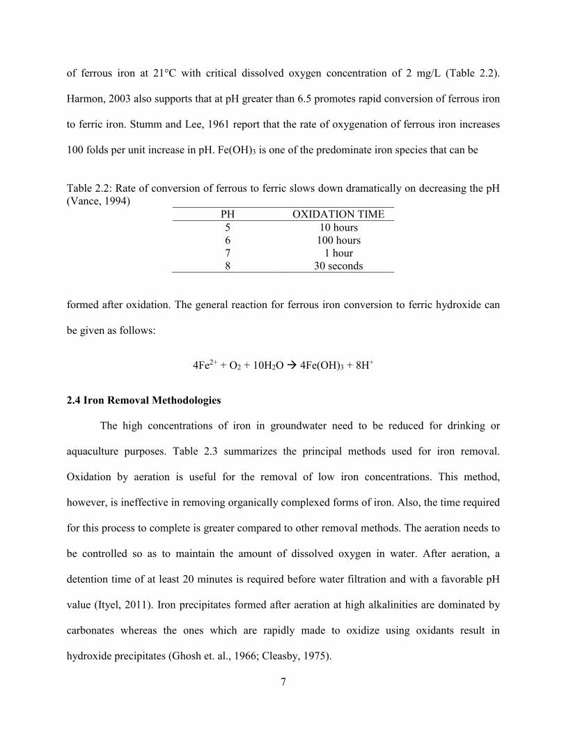
Table 2.2: Rate of conversion of ferrous to ferric slows down dramatically on decreasing the pH (Vance, 1994)

PH OXIDATION TIME 5 10 hours 6 100 hours 7 1 hour 8 30 seconds

formed after oxidation. The general reaction for ferrous iron conversion to ferric hydroxide can

be given as follows:

4Fe2+ + O2 + 10H2O 4Fe(OH)3 + 8H+

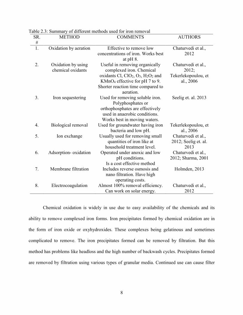
2.4 Iron Removal Methodologies

The high concentrations of iron in groundwater need to be reduced for drinking or

aquaculture purposes. Table 2.3 summarizes the principal methods used for iron removal.

Oxidation by aeration is useful for the removal of low iron concentrations. This method,

however, is ineffective in removing organically complexed forms of iron. Also, the time required

for this process to complete is greater compared to other removal methods. The aeration needs to

be controlled so as to maintain the amount of dissolved oxygen in water. After aeration, a

detention time of at least 20 minutes is required before water filtration and with a favorable pH

value (Ityel, 2011). Iron precipitates formed after aeration at high alkalinities are dominated by

carbonates whereas the ones which are rapidly made to oxidize using oxidants result in

hydroxide precipitates (Ghosh et. al., 1966; Cleasby, 1975).

8

Table 2.3: Summary of different methods used for iron removal SR. #

METHOD COMMENTS AUTHORS

1. Oxidation by aeration Effective to remove low concentrations of iron. Works best

at pH 8.

Chaturvedi et al., 2012

2. Oxidation by using chemical oxidants

Useful in removing organically complexed iron. Chemical

oxidants Cl, ClO2, O3, H2O2 and KMnO4 effective for pH 7 to 9.

Shorter reaction time compared to aeration.

Chaturvedi et al., 2012;

Tekerlekopoulou, et al., 2006

3. Iron sequestering Used for removing soluble iron. Polyphosphates or

orthophosphates are effectively used in anaerobic conditions. Works best in moving waters.

Seelig et. al. 2013

4. Biological removal Used for groundwater having iron bacteria and low pH.

Tekerlekopoulou, et al., 2006

5. Ion exchange Usually used for removing small quantities of iron like at

household treatment level.

Chaturvedi et al., 2012; Seelig et. al.

2013 6. Adsorption- oxidation Operated under anoxic and low

pH conditions. Is a cost effective method

Chaturvedi et al., 2012; Sharma, 2001

7. Membrane filtration Includes reverse osmosis and nano filtration. Have high

operating costs.

Holmden, 2013

8. Electrocoagulation Almost 100% removal efficiency. Can work on solar energy.

Chaturvedi et al., 2012

Chemical oxidation is widely in use due to easy availability of the chemicals and its

ability to remove complexed iron forms. Iron precipitates formed by chemical oxidation are in

the form of iron oxide or oxyhydroxides. These complexes being gelatinous and sometimes

complicated to remove. The iron precipitates formed can be removed by filtration. But this

method has problems like headloss and the high number of backwash cycles. Precipitates formed

are removed by filtration using various types of granular media. Continued use can cause filter

9

bed clogging which results in reduced filter efficiency and headloss problems. Frequent

backwash cycles are needed for efficient use of the filter.

Iron sequestering/ chelation is the combining of ferrous iron with other molecules so as to

avoid it from converting to ferric state. This, method can thus be used for treating groundwater

which has high concentrations of ferrous iron. It is cheap to install and easy to operate.

Sequestering agents used are phosphates, polyphosphates and sodium silicates. However, ferrous

iron is embedded by these agents into colloidal forms thus, complicating its removal (Robinson,

1990).

Biological removal has the advantage of having high filtration rates and no use of

chemical oxidants. Iron oxidizing bacteria like Gallionella, Crenothrix, Sphaerotilus and

Leptothrix perform the task of oxidation (Ankrah et al., 2009). A number of parameters affect the

biological removal process, like iron loading, type of oxidation occurring, pH, temperature and

co-precipitates formed. Typical conditions needed for successful biological iron removal include

a pH range of 6.5 to 7.2, low concentrations of dissolved oxygen, and temperatures ranging from

about 50°F to 75°F (Summerfelt, 1999).

Ion exchange resins can be used at any pH and their capacity can be recharged by using

proper regenerating solutions. These ions replace the contaminant ions with other acceptable

ions. It has the advantage of operating at varying flow rates but has no effect on water turbidity,

total solids and alkalinity, thus, limiting its use (General Electrical Company, 2012). Ion

exchange can be carried out for cations as well as anions using the opposite charged ions. An

ideal exchanger has characteristic hydrophilic structure, a rapid exchange rate and both chemical

and physical stability (Harland, 1994).

10

Adsorptive filtration is a cost effective process requiring no use of chemicals and also has

minimal sludge production in case of iron removal, since the iron adsorbed to the media particles

increases its surface area thus, providing more surface for adsorption. It applies the phenomenon

of adsorption which is the attachment of contaminant to the surface of media. Here the ferrous

iron is adsorbed to the media surface followed by its subsequent oxidation to ferric. Adsorption

can be used for purifying groundwater which usually has high levels of ferrous concentrations.

The treatment is very cheap and can be used in rural areas. This procedure is effective but is slow

(Vet et. al. 2011, Sharma 2001).

Membrane filtration applies to reverse osmosis, nano filtration, ultra-filtration and micro-

filtration. Membrane filters are used for delivering high quality effluent water (Holmden, 2013).

They provide a barrier for the many contaminant particles like solids, viruses, metal hydroxides,

oils, ions of specific size and emulsions. It is widely used in milk production industry, oil-water

separation, pharmaceutical and paint industry. These filters do not occupy much area and thus

have less installation costs.

2.5 Electrocoagulation and subsequent filtration of iron

An iron removal method that has proved to be effective in some applications is the

electrocoagulation (EC) process. The EC process has gained importance because of its high

removal efficiency, no use of chemicals, no secondary harmful disposal pollutant generation and

short treatment time. Common types of electrodes used for water treatment are aluminum and

iron. The electrocoagulation method using aluminum based electrodes is experimentally proving

to be a promising contaminant removal technique (Chen, 2004).

Coagulation has long been used in water purification/ treatment plants.

Electrocoagulation applies the same principles of coagulation except that the coagulant is added

11

by sacrificial electrodes instead of direct addition of chemical coagulants. Sacrificial anode

dissolves to generate coagulant which is made to mix rapidly in the water. The rapid mixing

caused charge neutralization of the contaminant species which help in their adsorption by

flocculation. Coagulants act as particle destabilizers by neutralizing the surface charge of

particles. Neutralization of charge is then followed by the activation of Van der Waals forces of

attraction which help in agglomeration of particles. In electrocoagulation, a sacrificial electrode

releases cations that act as a coagulant followed by floc formation which scavenges the iron

present in the solution. These flocs act as adsorption sites for iron removal. Here, the sacrificial

metal anode dissolves thus, generating the coagulant species. Immediate generation of hydrogen

can be seen on the cathode. The, ions released by the anode leads to metal hydroxides formation

which acts as adsorption sites for contaminants from water. Reactions occurring at anode and

cathode when using aluminum electrodes are as follows:

Anode: Al Al3+ + 3e-

2H2O 4H+ + O2 (g) + 4e-

Cathode: 3H2O + 2e- 2H2 (g) + 2OH-

(Comninellis et al., 2010; Sahu et al., 2014; Wang et al., 2010)

Oxygen evolution occurs at the anode due to simultaneous oxidation of water occurring in the

system. The hydrogen bubbles generated in the EC process can cause the floatation of flocs

formed. The dissolved anode and released hydroxyl ions react to form aluminum hydroxide

which precipitates out, the reaction can be given as:

Al3+ + 3H2O Al(OH)3 + 3H+

These aluminum hydroxide flocs act as adsorption site for iron.

12

Current application rates play a prominent role in the EC process (Mollah et al., 2004).

Depending of current passed, the contaminants are removed either by flotation or by

sedimentation. Low current promote sedimentation whereas, hydrogen gas production promotes

floc floatation at higher currents (Ghosh et al., 2008). The amount of Al3+ released in water on

passage of specific current is defined by Faraday’s law. Faraday’s law states that, “the mass of

substance produced or consumed is proportional to the quantity of charge passed”.

Thus,

1 F = 96484.56 C = 1 EW

Where;

F: Faraday’s constant

C: Coulombs (equivalent to 1 ampere-sec)

EW: Equivalent weight

EW = ��

�

Where,

n : valence of the ion

MW: Molecular weight

According to Faraday’s second law of electrolysis:

x (gm) = (�)(�)(��)

�����.����

Where;

x: mass of substance released or consumed in grams

A: Amount of current passed in Amperes

T: Time for which the current was passed in seconds

13

Thus, for aluminum electrodes, substituting the molecular weight of Aluminum as 26.981and

number of valence electrons as 3 in the above equation (1), we get the amount of Al released in

electrocoagulation as follows:

x mg-Al = (9.3216 X 10-2) (A) (T) ………………………………………………..……(1)

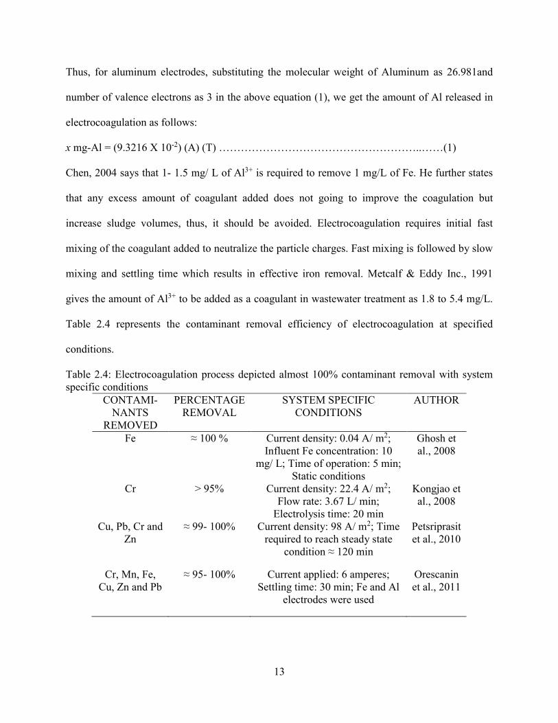
Chen, 2004 says that 1- 1.5 mg/ L of Al3+ is required to remove 1 mg/L of Fe. He further states

that any excess amount of coagulant added does not going to improve the coagulation but

increase sludge volumes, thus, it should be avoided. Electrocoagulation requires initial fast

mixing of the coagulant added to neutralize the particle charges. Fast mixing is followed by slow

mixing and settling time which results in effective iron removal. Metcalf & Eddy Inc., 1991

gives the amount of Al3+ to be added as a coagulant in wastewater treatment as 1.8 to 5.4 mg/L.

Table 2.4 represents the contaminant removal efficiency of electrocoagulation at specified

conditions.

Table 2.4: Electrocoagulation process depicted almost 100% contaminant removal with system specific conditions

CONTAMI-NANTS

REMOVED

PERCENTAGE REMOVAL

SYSTEM SPECIFIC CONDITIONS

AUTHOR

Fe ≈ 100 % Current density: 0.04 A/ m2; Influent Fe concentration: 10

mg/ L; Time of operation: 5 min; Static conditions

Ghosh et al., 2008

Cr > 95% Current density: 22.4 A/ m2; Flow rate: 3.67 L/ min;

Electrolysis time: 20 min

Kongjao et al., 2008

Cu, Pb, Cr and Zn

≈ 99- 100% Current density: 98 A/ m2; Time required to reach steady state

condition ≈ 120 min

Petsriprasit et al., 2010

Cr, Mn, Fe, Cu, Zn and Pb

≈ 95- 100% Current applied: 6 amperes; Settling time: 30 min; Fe and Al

electrodes were used

Orescanin et al., 2011

14

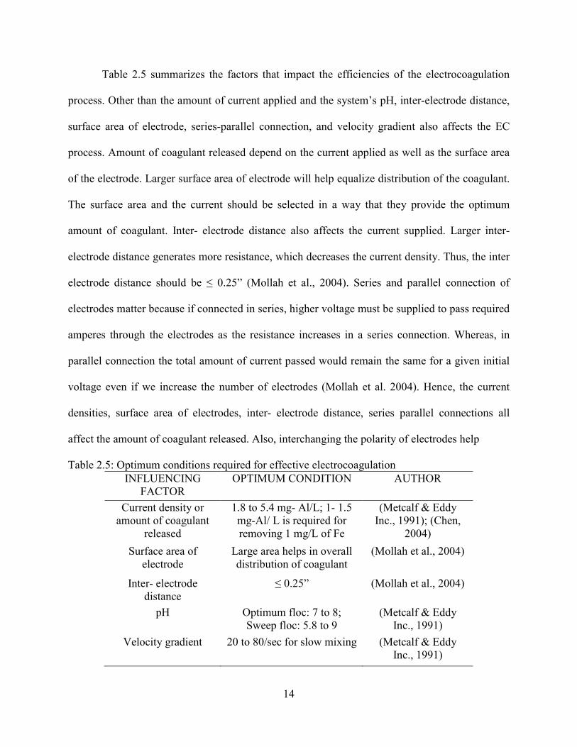
Table 2.5 summarizes the factors that impact the efficiencies of the electrocoagulation

process. Other than the amount of current applied and the system’s pH, inter-electrode distance,

surface area of electrode, series-parallel connection, and velocity gradient also affects the EC

process. Amount of coagulant released depend on the current applied as well as the surface area

of the electrode. Larger surface area of electrode will help equalize distribution of the coagulant.

The surface area and the current should be selected in a way that they provide the optimum

amount of coagulant. Inter- electrode distance also affects the current supplied. Larger inter-

electrode distance generates more resistance, which decreases the current density. Thus, the inter

electrode distance should be ≤ 0.25” (Mollah et al., 2004). Series and parallel connection of

electrodes matter because if connected in series, higher voltage must be supplied to pass required

amperes through the electrodes as the resistance increases in a series connection. Whereas, in

parallel connection the total amount of current passed would remain the same for a given initial

voltage even if we increase the number of electrodes (Mollah et al. 2004). Hence, the current

densities, surface area of electrodes, inter- electrode distance, series parallel connections all

affect the amount of coagulant released. Also, interchanging the polarity of electrodes help

Table 2.5: Optimum conditions required for effective electrocoagulation INFLUENCING

FACTOR OPTIMUM CONDITION AUTHOR

Current density or amount of coagulant

released

1.8 to 5.4 mg- Al/L; 1- 1.5 mg-Al/ L is required for removing 1 mg/L of Fe

(Metcalf & Eddy Inc., 1991); (Chen,

2004)

Surface area of electrode

Large area helps in overall distribution of coagulant

(Mollah et al., 2004)

Inter- electrode distance

≤ 0.25” (Mollah et al., 2004)

pH Optimum floc: 7 to 8; Sweep floc: 5.8 to 9

(Metcalf & Eddy Inc., 1991)

Velocity gradient 20 to 80/sec for slow mixing (Metcalf & Eddy Inc., 1991)

15

improve the process performance since, both the electrodes alternatingly act as the sacrificial

anodes.

The next factor affecting the process is pH. High pH favors efficient iron removal since it

accelerates oxidation of iron. Metcalf & Eddy Inc., 1991 gives the range for optimum and sweep

floc formation when using aluminum as the coagulant. A pH between 7 to 8 results in optimum

floc formation and is supposed to remove the contaminants most effectively. The overall pH

range for aluminum hydroxide floc formation has been given as 5.8 to 9. Electrocoagulation

generally operates best at a near neutral pH. At acidic pH i.e. ≤ 3, iron and aluminum are soluble,

hence do not allow coagulation. The hydrogen is released as H2 gas, helping in electro- flotation.

OH- results in metal hydroxide formations.

Rapid mixing and slow mixing in the coagulation step depends on the velocity gradient

(G) applied. The G values are usually given by the manufacturer and are instrument specific.

Initial fast mixing results in neutralization of contaminant particles which helps them to cluster

together. Fast mixing is then followed by continuous slow mixing which further help in

agglomeration and flocculation. Slow mixing in water treatment plants using aluminum requires

a G-value between 20-80 per sec (Metcalf and Eddy Inc., 1991).

The flocs formed by electrocoagulation can then be removed by filtration. Different

filtration media can be used for removing the iron flocks generated by EC. Oldest media in use is

sand. Sand filters are cheap and require low maintenance, hence can be installed in rural areas.

Bed depth for sand filters normally ranges between 24 to 36 inches. Sand media carries a

negative surface charge which can attract contaminant cations. Positive iron ions get adsorbed to

the negatively charged sand surface and are removed from the water. Continuous usage of sand

filter can also result in a biomat layer formation on the top surface of the media which causes the

16

clogging. Sand filter maintenance needs to be done by a trained person since; it requires raking

or sometimes removing the top layer of media as it gets clogged after continuous usage (Taylor

et. al, 1997).

Polyethylene plastic floating beads have recently gained importance for removing metals

from water. The diameter of these polyethylene beads are typically 2- 3mm. Floating bead media

are known to be effective in removing particles as small as 50 microns (Ahmed, 1996). These

beads have a specific gravity of 0.92 gm/ cm3, which is slightly less than that of water. The

floating bead media works effectively when installed as an up-flow filter. The polyethylene

floating bead has almost negligible surface charge thus, not helping directly for adsorption of

ions on its surface. Another important media property is its surface area. Larger the surface area,

larger is the surface availability for adsorption. The polyethylene beads provide high surface area

that is required for the filtration process. Traditionally used sand filters have to deal with

problems of fouling and high water loss during backwashing. To deal with this problem of

backwashing water loss, specialized bead filters were developed and are preferred over the other

media for filtration of recirculating aquaculture system waters (Malone et al., 1993, Sastry et. al.,

1999).

2.6 Adsorption- Oxidation iron removal method

In the adsorption oxidation technique, ferrous first gets adsorbed to the filter media

before it gets oxidized to ferric hydroxide. Surface charges and interaction between the adsorbate

and the adsorbing surface are the major factors affecting the adsorption. Examples of some solids

used as adsorbents are activated carbon, ion exchange resins and oxides of aluminum and iron.

Sharma, 2001 in his research tested iron removal using basalt, anthracite, olivine, magnetite,

virgin sand, iron oxide coated sand, pumice and limestone. He found that basalt displayed

17

highest adsorption amongst the virgin materials tested. He also concluded that, iron oxide coated

sands had higher adsorption capacity than the virgin sand. The coated sand had a large specific

area and higher porosity thus, making it more effective in adsorption compared to virgin sand.

He noted as the coating increased, the media’s grain size increased while its density decreased. A

floating bead filter installed in New Roads, Louisiana on a well in the Mississippi river alluvium

failed due to heavy iron coat formation around the beads. The coating formed increased the

specific gravity of the beads, thus, making them sink. This coating of beads can be recognized as

the fact that adsorption must have occurred which gave rise to the heavy coat formation.

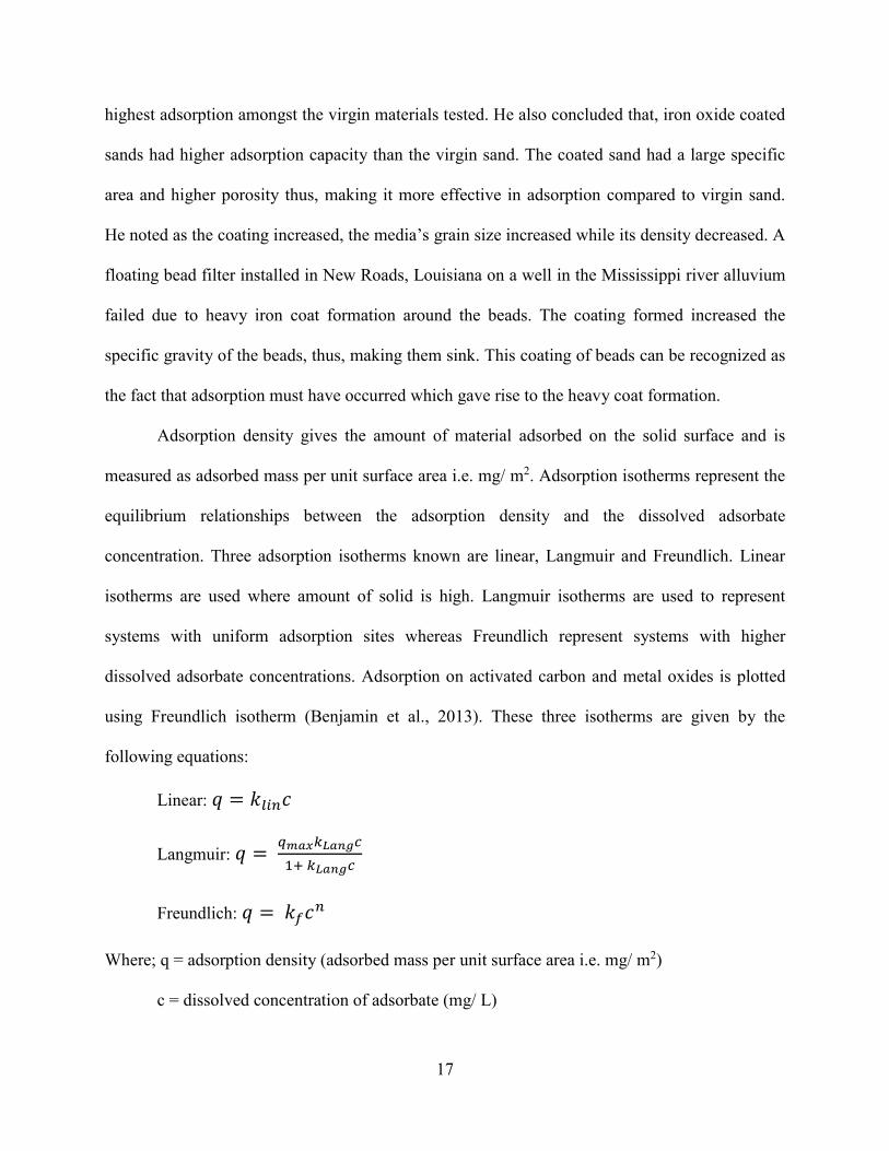
Adsorption density gives the amount of material adsorbed on the solid surface and is

measured as adsorbed mass per unit surface area i.e. mg/ m2. Adsorption isotherms represent the

equilibrium relationships between the adsorption density and the dissolved adsorbate

concentration. Three adsorption isotherms known are linear, Langmuir and Freundlich. Linear

isotherms are used where amount of solid is high. Langmuir isotherms are used to represent

systems with uniform adsorption sites whereas Freundlich represent systems with higher

dissolved adsorbate concentrations. Adsorption on activated carbon and metal oxides is plotted

using Freundlich isotherm (Benjamin et al., 2013). These three isotherms are given by the

following equations:

Linear: � = �����

Langmuir: � = ����������

��������

Freundlich: � = ����

Where; q = adsorption density (adsorbed mass per unit surface area i.e. mg/ m2)

c = dissolved concentration of adsorbate (mg/ L)

18

Klin, kLang, kf, qmax and n = empirical constants

The adsorption capacity depends on the dissolved oxygen content, pH, surface area of

filter media and its surface charge (Table 2.6). Dissolved oxygen content of water to be treated

should be close to zero so as to prevent oxidation of ferrous to ferric. To encourage the

adsorption-oxidation mechanism it is necessary to maintain the pH around 6.5 so as to inhibit

oxidation. This provides time for adsorption of ferrous to filter media before it gets oxidized to

ferric. Most groundwater are anoxic with low pH; conditions which favors the ferrous state. This

removal approach can hence be used for treating groundwater in rural areas where high operating

costs need to be avoided. Larger surface area provides more surface for adsorption. Increased

surface area of coated sand is the reason for its increased adsorption capacity. The ferric

hydroxide precipitate has a positive surface charge at neutral pH, to which the OH – gets attracted

which results in a localized pH increase near the particle surface. This rise in pH, accelerates the

conversion of adsorbed ferrous iron to the ferric hydroxide flocs; a possible explanation to the

increased adsorption capacity of iron coated sands (Sharma 2001). Sharma, 2001 also had

concluded that, increasing concentrations of Ca2+ decreases the iron adsorption capacity whereas

the iron adsorption was seen to be increased when SO42- concentration were increased. Presence

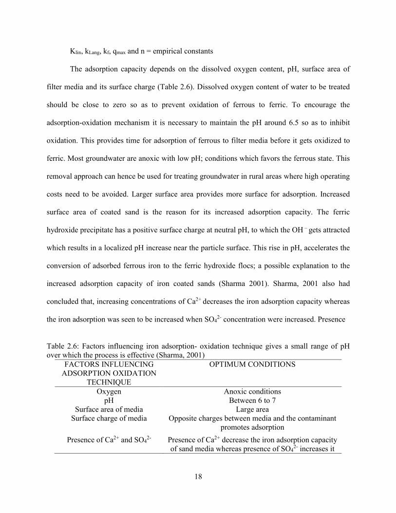
Table 2.6: Factors influencing iron adsorption- oxidation technique gives a small range of pH over which the process is effective (Sharma, 2001)

FACTORS INFLUENCING ADSORPTION OXIDATION

TECHNIQUE

OPTIMUM CONDITIONS

Oxygen Anoxic conditions pH Between 6 to 7

Surface area of media Large area Surface charge of media Opposite charges between media and the contaminant

promotes adsorption

Presence of Ca2+ and SO42- Presence of Ca2+ decrease the iron adsorption capacity

of sand media whereas presence of SO42- increases it

19

of SO42- also decreases the rate of conversion of ferrous to ferric and thus, boosts the adsorption

of ferrous on the media (Sung & Morgan, 1980).

20

CHAPTER 3: PRELIMINARY STUIDIES

3.1 Introduction

Preliminary studies tested the iron removal efficiency of floating bead bed on passage of

electrocoagulated contaminant water through a bead bed. These studies established a baseline for

effects of control variables on the iron removal efficiency. Current and flow rates are known to

affect the electrocoagulation and filtration process. Thus, different currents and flow rates were

tried here. The pH was kept constant and within range for sweep floc formation. Coagulation and

flocculation were combined in one step in the coagulation tank. Initial fast mixing on starting the

current was followed by continuous slow mixing by inducing air in the coagulation tank.

Coagulation- flocculation was followed by filtration through polyethylene floating bead bed.

Based on the results obtained, few design changes were installed and the removal

efficiencies were reanalyzed. The design changes installed were statistically checked to confirm

if they have any significant effect on iron removal.

3.2 Materials and methods

The setup comprised of a coagulation tank and a floating bead bed column (Figure 3.1).

The coagulation tank was made of clear PVC of 5” ID and stood 36” tall. Water was circulated

from the coagulation tank to the floating bead bed column using a ¾” ID hose. The floating bead

column was made using clear PVC pipe with 4” ID and was 34” in height. The outlet of this

column directed the water back to the coagulation tank forming a recirculating system. This

column was filled in with 10” deep polyethylene floating bead media having size 2-3 mm. These

beads have a specific gravity of 0.92 gm/cm3. Water was circulated using a 1/50 HP centrifugal

pump (Little giant 3X-MDX).

21

Figure 3.1: Schematic representation of the setup used for running preliminary set of experiments: centrifugal pump is positioned before the bead bed

Aluminum base electrodes having dimension 1-1/2” X 1/16” X 34” were used for

electrocoagulation (Figure 3.2). Total submersed surface area of one electrode was 0.71 ft2

(0.066 m2) (2 faces x 1-1/2" x 34”). Mastech DC power source (HY3010D) was used here. pH

was measured using Hach HQ411d pH/mV meter. Samples collected were analyzed with Hach’s

22

DR 2800 spectrophotometer. The last sample obtained in all the experiments was also run

through 25 mm GD/X Whatman (91816A) filter. Air is blown in the coagulation tank for the

purpose of mixing. To limit the size of air bubbles created, air stone was installed along with an

inflow controller on the air pump. This generated smaller sized bubbles which would help in

flocculation and won’t tear up the floc. Experimental setup consisting of electrocoagulation tank

and filtration column is given in Figure 3.3.

Figure 3.2: Aluminum electrodes were constructed from aluminum stock having dimensions 1-

1/2” X 1/16” X 48”, with submerged length of 34”

23

Figure 3.3: Experimental setup consisting of electrocoagulation tank and filtration column

Figure 3.1 has emphasized the position of the pump. High velocity gradient in the system

is expected to cause shearing of floc. Centrifugal pumps have velocities higher than 80 per sec

which is the maximum limit for slow mixing. Placement of pump between the coagulation tank

and the bead bed was thus suspected to be responsible for floc shearing before it can get captured

in the bead bed. Later the pump was moved after the bead bed (Figure 3.4). The experiment was

then re-run at combinations of current and flow rate.

24

Figure 3.4: Schematic representation of the electrocoagulation and bead bed column system: centrifugal pump is positioned after the bead bed to avoid any floc breakage caused by the high velocity gradient of the pump

25

Water set to pH 8±0.5 using NaHCO3 was allowed to set overnight in a 50 gallon vessel.

The coagulation tank was filled in with this water and was circulated through the system with

continuous aeration. The water temperature was set to 25°C using water heater (Aqueon

E308548). The flow rate was then set to desired recirculating flow. Three different flow rates

(flux rates) were tested in these experiments which were 0.33 gpm (3.79 gpm/ ft2), 0.66 gpm

(7.58 gpm/ ft2) & 1.32 gpm (15.17 gpm/ ft2). Iron was added in the coagulation tank as ferric

chloride (FeCl3), to a level of 7.1 mg-Fe/ L. One minute mixing of iron in the coagulation tank

was allowed before starting the current. The three currents tested were 1, 3 and 6 amperes which

releases 167.78, 503.36, 1006.732 mg-Al for total system volume of 17.92 liters (equivalent to

9.4, 28.1 and 56.2 mg-Al/ L respectively) according to Equation 1. Table 3.1 gives the time for

which the various currents should be passed so as to generate 5.4 mg/L of coagulant. The

experiments though, were run with the current supplied for full 30 minutes.

Table 3.1: Time required to generate specified amount of aluminum coagulant is inversely proportional to the amperes applied

AMPERES APPLIED TO RELEASE 5.4 MG/L OF ALUMINUM IN 17.92 L

OF WATER

TIME FOR WHICH THE CURRENT IS PASSED (IN

MINUTES) 1 17.3 3 5.77 6 2.88

Combinations of the three flow rates and currents were run for 30 minutes each. The

combinations were selected using random number generator in ExcelsTM and were run

accordingly. Samples were collected after every 10 minutes for the 30 minute runs. System was

cleaned after every run using manual backwashing. Electrodes were cleaned using sand paper,

followed by acetone wash after every six runs.

26

Samples collected were read using EPA verified Hach method 8008 used for sample

preparation and analysis of total iron. The spectrophotometer Hach DR2800 was first calibrated

by plotting calibration curves. Hach’s Iron Standard Solution, 10 mg/L as Fe (NIST) was used

for preparing the calibration curves. The calibration was triplicated to obtain an estimate of

measurement error. EPA has three approved techniques for plotting calibrations, namely; linear

calibration through origin, linear least squares regression and weighted least squares regression.

Linear calibration through origin technique was used here. The method can be accepted when the

standard deviation obtained for the mean calibration factor (CF) or the mean response factor

(RF) is ≤ 20%. The intercept here was not set to zero so as to find out the correction in

measurement. Dilutions made were 0, 0.5,1, 1.5 and 2 mg-Fe/L. Deionized water was used here.

Instrument calibration is important for obtaining precise results. All instruments used

which are pH meter and spectrophotometer were calibrated before usage. Calibration of the

spectrophotometer Hach’s DR2800 gave an intercept correction of 0.136 mg-Fe/ L when the

triplicate of calibration curves were plotted. Figure 3.5 gives the average of calibrations carried

out to find the measurement error.

Reagent blanks are measured to find out the iron content already present in the solution

read as blank. The reagent blank value may change per day, though usually remains the same.

Reagent blank was measured every day before taking the readings. The reagent blank value

consistently obtained about 0.03 mg-Fe/L. This was also used towards finding out the correction

to be applied. The total measurement error applied towards all the iron concentrations read was

thus sum of the measurement error (0.136 mg-Fe/ L) and the reagent blank (0.03 mg-Fe/ L)

equaling to 0.166 mg-Fe/ L.

27

Figure 3.5: Average plot of three calibrations estimated the measurement error of 0.136 mg-Fe/ L for spectrophotometer Hach DR2800 3.3 Results and discussion

Preliminary studies were run to get an idea of how the current and flow rate affect the

iron removal efficiencies. Thus, the experiments here were not triplicated. Following set of

graphs (Figure 3.6) depict the removal efficiencies obtained at the three currents and flow rates

applied. The conditions tested in these runs did not give the expected iron removal of less than 1

mg-Fe/ L. Intercept was set to 7.1 (mg- Fe/ L) for obtaining the decay rates (Table 3.2). The

decay rates given in Table 3.2 were hardly different from each other and the data was not

triplicated and all decay rates being low, no trend could be described.

y = 1.1482x + 0.1366R² = 0.994

0.00

0.50

1.00

1.50

2.00

2.50

3.00

0 0.2 0.4 0.6 0.8 1 1.2 1.4 1.6 1.8 2

Co

nce

ntr

atio

n (

mg-

Fe/L

)

Dilutions (mg-Fe/L)

Calibrations Average

28

Figure 3.6: First trial of iron removal obtained for three flow rates at aluminum dosage of 9.4, 28.1 and 56.2 mg-Al/ L failed to drop the iron concentrations below 1 mg- Fe/ L

0

1

2

3

4

5

6

7

0 10 20 30

Co

nce

ntr

atio

n m

g-Fe

/L

Time in minutes

Residual Fe at 9.4 mg-Al/L

0.33gpm

0.66gpm

1.32gpm

0

1

2

3

4

5

6

7

0 10 20 30

Co

nce

ntr

atio

n m

g-Fe

/L

Time in minutes

Residual Fe at 28.1 mg-Al/L

0.33gpm

0.66gpm

1.32gpm

0

1

2

3

4

5

6

7

0 10 20 30

Co

nce

ntr

atio

n m

g-Fe

/L

Time in minutes

Residual Fe at 56.2 mg-Al/L

0.33gpm

0.66gpm

1.32gpm

29

Table 3.2: Decay rates for all combinations of currents and flow rates run for preliminary studies showed no difference

CURRENT (AMPERES)

FLOWRATE (GPM)

DECAY RATE (MIN-1)

1 0.33 0.04346 1 0.66 0.03633 1 1.32 0.0322 3 0.33 0.04139 3 0.66 0.03933 3 1.32 0.04562 6 0.33 0.03416 6 0.66 0.03554 6 1.32 0.04276

Some of the experiments above were run continuously for three hours, though the current

was stopped after 30 minutes. This was done to check if the concentration drops down after 30

minutes. The trials were done for a constant flow rate of 1.32 gpm (15.17 gpm/ft2) and currents

of 1 and 3 amperes. The data was confirmed by running triplicates. The results obtained are

shown in Figure 3.7. Decay rates were almost same. The iron removal graphs indicate an

exponential decay curve. Thus, the statistics run compared the decay rates obtained for every

experiment.

A possible problem leading to inefficient removal of iron from the water within 30

minutes of run might be because of floc breakage by the centrifugal pump (Figure 3.1). The high

velocity gradient in the pump was suspected of tearing up the floc that formed in the coagulation

tank thus, not dropping the iron concentration below 1 mg-Fe/ L. The recirculation pump was

placed after the filtration bed as shown in Figure 3.4 and results for selected runs were

reexamined. Flow rate used was 0.33 gpm and current applied was 1 and 6 amperes.

30

Figure 3.7: Triplicated experiments run for 180 minutes lowered the iron concentration to about 0.5 mg-Fe/L. Current was supplied for first 30 minutes only

Experimental runs for these combinations of currents and flow rates were triplicated for

the pump positioned before the bead bed as well. Figure 3.8 compares the iron removal obtained

at the two pump positions. From the graph and ANOVA run on the data obtained proved that the

position of pump affected the removal efficiency. The p- value for major effect of pump position

on concentration was 0.0036 showing significance though combined effect of pump position and

current was not significant since the p-value was greater than 0.05. List of decay rates referring

to Figure 3.8 are given in Table 3.2.

y = 7.1e-0.019x

y = 7.1e-0.018x

0

1

2

3

4

5

6

7

0 30 60 90 120 150 180

Co

nce

ntr

atio

n m

g-Fe

/L

Time in minutes

Residual Fe at 1.32 gpm

9.36 mg-Al/L

28.09 mg-Al/L

Expon. (9.36 mg-Al/L)

Expon. (28.09 mg-Al/L)

31

Figure 3.8: Iron removal comparison between A & B at a constant flow rate of 0.33 gpm and currents of 1A (9.4 mg-Al/ L) and 6A (56.2 mg-Al/ L). Where, A represents the position of pump placed after the bead bed and B represents the position of pump before bead bed

0

1

2

3

4

5

6

7

0 10 20 30

Co

nce

ntr

atio

n m

g-Fe

/L

Time in minutes

Residual Fe at 9.4 mg-Al/L

A

A

A

B

B

B

0

1

2

3

4

5

6

7

0 10 20 30

Co

nce

ntr

atio

n m

g-Fe

/L

Time in minutes

Residual Fe at 56.2 mg-Al/L

A

A

A

B

B

B

32

Decay rate for experiments run with the pump placed after the bead bed column were

higher than those when the pump was before bead bed by about 1.25 times (Table 3.3).

Table 3.3: Decay rates for Figure 3.8 depicting an increase in iron removal efficiency by about 1.25 times on moving the pump’s position after bead bed CURRENT

(AMP) FLOWRATE

(GPM) PUMP

POSITION DECAY RATE

(MIN-1) AVERAGE DECAY

RATE (MIN-1)

1 0.33 B 0.04346 0.03958

1 0.33 B 0.03851

1 0.33 B 0.03678

6 0.33 B 0.03416 0.03993

6 0.33 B 0.03839

6 0.33 B 0.04723

1 0.33 A 0.04241 0.04608

1 0.33 A 0.04706

1 0.33 A 0.04876

6 0.33 A 0.0543 0.05341

6 0.33 A 0.05089

6 0.33 A 0.05505

3.4 Conclusions

It can be concluded that, the parameters tested in the preliminary studies did not show

any significant difference in the removal efficiencies. To confirm the statistical significance of

the effect of current, pH and flow rate, the above combinations of currents and flow rates need to

be triplicated. Preliminary studies confirmed that the pump’s position affected the removal

efficiency significantly since the p- value obtained after running ANOVA was less than 0.05.

The samples collected at the end of experiment were also read after filtering them

through 25mm GD/X Whatman filter. It was observed that the all these readings were below 0.3

mg-Fe/ L. We can hence conclude that the iron being read in all the graphs is basically in

particulate form which is not forming larger flocs and thus not being removed by the bead bed.

33

Running the experiment for continuous three hours allowed for multiple passes through the bead

bed achieving the objective of bringing the iron content down to 0.3 mg-Fe/ L.

34

CHAPTER 4: IRON REMOVAL EFFECIENCY OF A FLOATING BEAD BED BY APPLICATION OF ELECTROCOAGULATION

4.1. Introduction

Aquaculture requires high quality water for maintaining healthy stock. Most fish species

not being tolerant to high iron concentrations generates the need of supplying high quality water.

The aquaculture industry utilizes about 3% of Louisiana’s groundwater (USGS, 2005). To

increase the groundwater usage in aquaculture, efficient iron removal needs to be achieved. The

water must be treated in smallest treatment time possible; otherwise, large storage tanks need to

be installed.

Electrocoagulation is a developing technique being applied to water purification.

Effective contaminant removal, shorter reaction times, no oxidation chemicals are some of the

benefits associated with electrocoagulation. Coagulant is released from a sacrificial anode.

Common electrodes used are iron and aluminum. The process of electrocoagulation causes

particle destabilization that leads to floc formation. The flocs formed can then be filtered out

from the system.

Filtration media used, its surface area, size, surface charge all decide its contaminant

removal efficiency. Polyethylene floating beads sized 2-3 mm have the high surface area

required to facilitate iron removal. Specific gravity of these beads being lower than water makes

them float. Removal efficiency of this media thus works best when installed in an up flow

filtration system. Objective of this chapter was to drop down the iron concentrations to about 0.3

mg-Fe/ L by applying electrocoagulation.

35

4.2 Background

Aquaculture involves commercial fish raising under controlled environment.

Recirculating aquaculture systems require regular cleaning of water since it is being reused. If

factors like dissolved oxygen, salinity, pH and contaminant levels are not monitored and

controlled, it might result in harming the fish. Most species of fish cannot tolerate iron

concentrations above 0.5 mg-Fe/L (Buttner et al., 1993).

Various water purification methods like chemical oxidation, iron sequestering, biological

removal, ion exchange and membrane filtration are in use for removing iron. Some of these

methods are costly while some require high quantity of chemicals. A developing technique,

electrocoagulation, is showing high removal efficiencies for various contaminants like Cr, Mn,

Fe, Cu, Zn and Pb (Orescanin et al., 2011; Petsriprasit et al., 2010). Removal efficiencies being

in the range of 90- 100%. Electrocoagulation makes use of sacrificial metal electrode which

would release coagulant ions in the solution on passage of electric current. Iron and aluminum

are the most commonly used electrode materials.

Electrocoagulation follows the same theory of coagulation using chemical coagulants like

alum, ferric chloride and others except that electrocoagulation directly adds in the coagulating

ions. Coagulation is usually followed by a flocculation time which is important for forming

dense flocs. The denser the flocs, higher are its chances of being captured in the filtration bed.

Various filtration media are known to be in use, like, sand, granular activated carbon, manganese

greensand, ion exchange resins. Another high efficiency media consists of polyethylene floating

beads with a specific surface area of about 1050- 1300 m2/ m3 (Ahmed, 1996). Larger the surface

area of media, higher will be their ability of solid capturing. These beads have specific gravity of

about 0.92 gm/cm3.

36

Other factors affecting the electrocoagulation and filtration process are pH, mixing and

flow rates. Metcalf & Eddy Inc., 1991 has given the overall pH range for aluminum hydroxide

floc formation as 5.8 to 9. Lower pH < 3 will result in high solubility of iron and aluminum, thus

not supporting coagulation. Coagulation and flocculation require rapid and slow mixing

respectively for first, overall dispersing of coagulant and second, agglomeration of flocs. Flow

rates to the bead bed also affect its solids removal efficiency. Low flow rates help in higher solid

capture (Ahmed, 1996).

Continuous operation of the system increases the amount of solids accumulated in the

bead bed. Interstitial velocity in filter bed increases with increase in particle accumulation. The

solids accumulated keep on moving upwards through the filter bed along with the flow of water

due to shearing of adsorbed particles or lack of attachment. After a certain time, these particles

might cross the bead bed and recirculate in the system. This is termed as ‘breakthrough’. When

breakthrough occurs, the captured contaminant particles move into clean water. It thus, becomes

necessary to monitor this point of breakthrough. Backwashing the bead bed before it reaches this

breakthrough point will help in continuous supply of clean water (Benjamin et al., 2013; EPA,

1995).

4.3 Materials and methods

The experimental setup included a coagulation tank connected to the filter column, both

constructed using a clear acrylic PVC with internal diameters 5” and 4” respectively. The total

volume of water in the system was 17.92 liters. The schematic representation of the setup used in

this experiment is given in Figure 4.1. Water was circulated in this recirculating system using a

1/50 HP centrifugal pump (Little giant 3X-MDX). Fresh/new polyethylene floating beads were

added to the filter column. These beads have a specific gravity of 0.92 gm/cm3. Bead bed’s depth

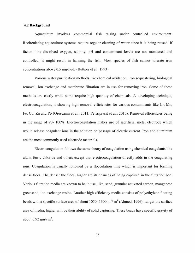
37

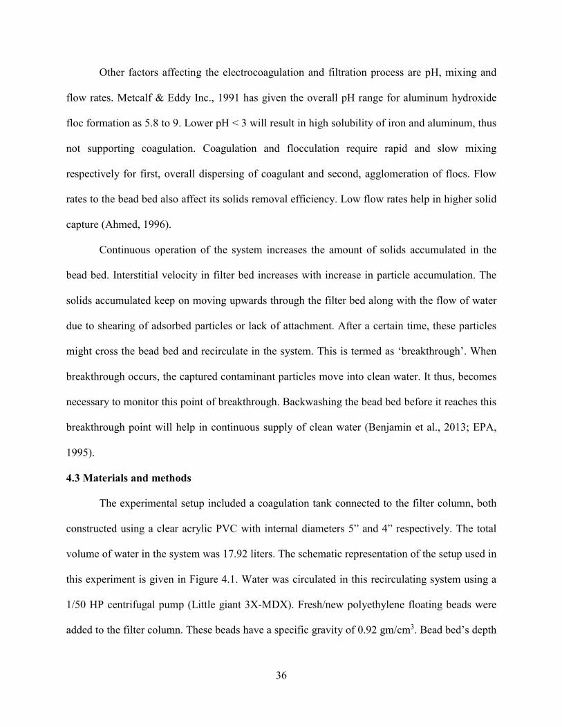
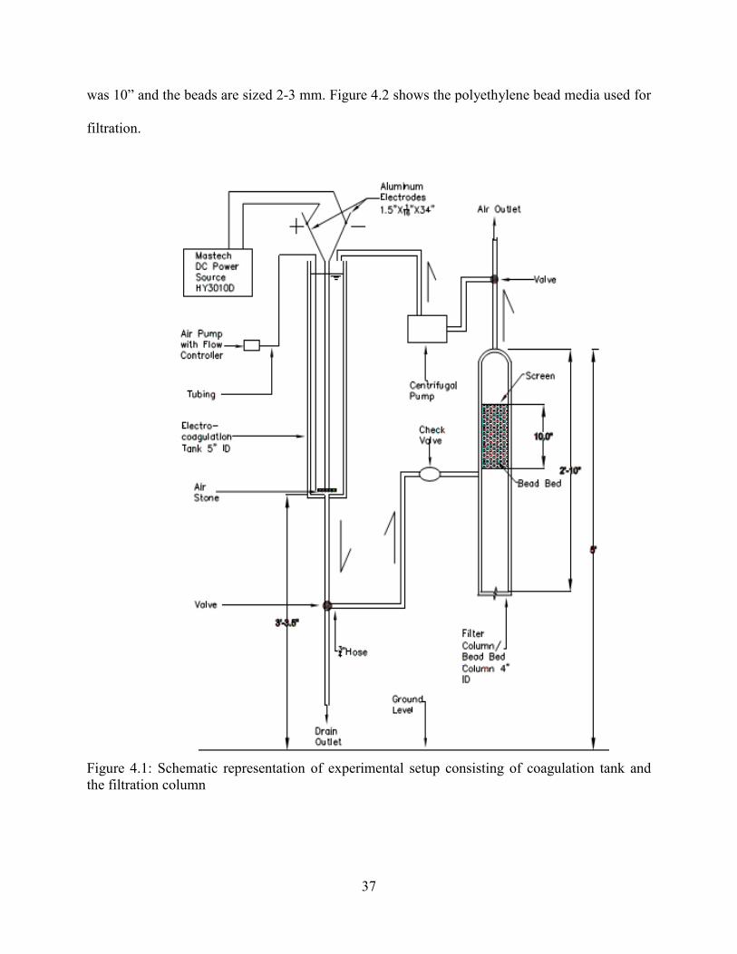
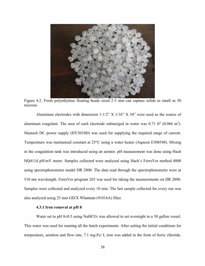
was 10” and the beads are sized 2-3 mm. Figure 4.2 shows the polyethylene bead media used for

filtration.

Figure 4.1: Schematic representation of experimental setup consisting of coagulation tank and the filtration column

38

Figure 4.2: Fresh polyethylene floating beads sized 2-3 mm can capture solids as small as 50 microns

Aluminum electrodes with dimension 1-1/2” X 1/16” X 34” were used as the source of

aluminum coagulant. The area of each electrode submerged in water was 0.71 ft2 (0.066 m2).

Mastech DC power supply (HY3010D) was used for supplying the required range of current.

Temperature was maintained constant at 25°C using a water heater (Aqueon E308548). Mixing

in the coagulation tank was introduced using an aerator. pH measurement was done using Hach

HQ411d pH/mV meter. Samples collected were analyzed using Hach’s FerroVer method 8008

using spectrophotometer model DR 2800. The data read through the spectrophotometer were at

510 nm wavelength. FerroVer program 265 was used for taking the measurements on DR 2800.

Samples were collected and analyzed every 10 min. The last sample collected for every run was

also analyzed using 25 mm GD/X Whatman (91816A) filter.

4.3.1 Iron removal at pH 8

Water set to pH 8±0.5 using NaHCO3 was allowed to set overnight in a 50 gallon vessel.

This water was used for running all the batch experiments. After setting the initial conditions for

temperature, aeration and flow rate, 7.1 mg-Fe/ L iron was added in the form of ferric chloride.

39

Three different flow rates tested in these experiments were 0.33 gpm (3.79 gpm/ ft2), 0.66 gpm

(7.58 gpm/ ft2) & 1.32 gpm (15.17 gpm/ ft2). One minute mixing of iron in the coagulation tank

was allowed before starting the current. Current of 1, 3 and 6 ampere were selected. The current

was applied throughout the run time of the experiment which was 30 minutes. These current of 1,

3 and 6 amperes applied for 30 minutes release 9.4, 28.1 and 56.2 mg-Al/ L respectively

according to Equation 1. The experiments were triplicated and the combination of current and

flow rate to be run was selected using ExcelsTM random number generator. Polarity of electrodes

was interchanged for every run. System was cleaned after every run using manual backwashing.

Electrodes were cleaned using sand paper, followed by acetone wash after every six runs to

remove the depositions from electrode plates. Data obtained and statistical analysis is given in

the results and discussion.

4.3.2 Iron removal at pH 6

A 50 gallon vessel was filled with water and 2 N hydrochloric acid was also added to this

water to drop its pH down to 6±0.5. This water was allowed to set overnight. The filter bed was

properly cleaned by manual back- flushing before starting every experimental run. Water from

the 50 gallon vessel was allowed to flow to the coagulation tank and the filter column. Air supply

and water heater placed in the coagulation tank were turned on. Heater’s temperature was set to

25°C. Iron removal at two flow rates, 0.33 gpm and 1.32 gpm was tested. The retention time in

coagulation tank provided by these flow rates were 14.34 and 3.58 min for 0.33 gpm and 1.32

gpm respectively. Aluminum electrodes were then immersed in the coagulation tank and were

connected to the DC power source. After having the initial conditions of pH and temperature set

to required values, 7.1 mg- Fe /L was added to the water tank in the form of ferric chloride. The

experiments were run in batch. The current was set to desired value. The currents applied in

40

these experiments were 1 and 6 amperes which released 9.4 mg-Al/ L and 56.2 mg-Al/ L

respectively over a 30 minute period. Flash mixing was allowed for proper mixing of

contaminant and coagulant in the coagulation tank. After one minute of flash mix, the system

was kept on slow aeration. Combinations of currents and flowrates were selected using ExcelsTM

random number generator.

4.4 Results and discussion

Iron concentrations were analyzed after every 10 minutes during the experiment. The

results and discussion section is divided into three parts, first representing the removal obtained

at pH 8; second, removals obtained at pH of 6 and third section gives the comparison of iron

removals for pH 8 and 6.

4.4.1 Iron removal at pH 8

Iron concentrations measured were plotted against time for all combinations of currents

and flow rates. Iron concentrations measured after every 10 minutes when the current applied

were 1, 3 and 6 amperes were plotted at varying flowrates (Figure 4.3). Analysis of variance

(ANOVA) was run on the data obtained. The p- values obtained for current, flowrate and

combined effect of current and flowrate were 0.09, 0.16, 0.51 respectively, which being > 0.05

are not significant. The range of coagulant dosed was already higher than the maximum amount

of coagulant required. This might be the reason towards the insignificance obtained for effect of

current on the concentration. Decay rates given in Table 4.1 showed no distinguishing pattern.

The flowrates were selected over a wide range, thus, providing varying retention times for

dispersion of coagulant and subsequent floc formation in the coagulation tank. It is important to

provide enough flocculation time, so as to form larger flocs which can be easily caught by the

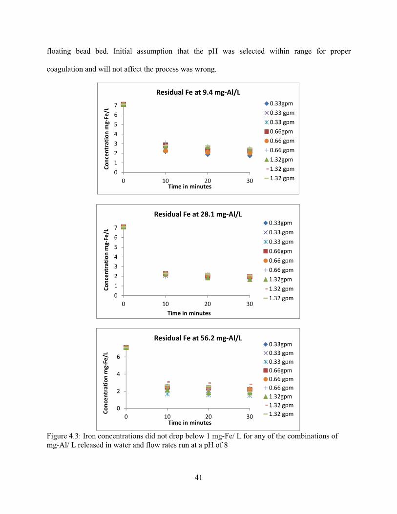
41

floating bead bed. Initial assumption that the pH was selected within range for proper

coagulation and will not affect the process was wrong.

Figure 4.3: Iron concentrations did not drop below 1 mg-Fe/ L for any of the combinations of mg-Al/ L released in water and flow rates run at a pH of 8

0

1

2

3

4

5

6

7

0 10 20 30

Co

nce

ntr

atio

n m

g-Fe

/L

Time in minutes

Residual Fe at 9.4 mg-Al/L

0.33gpm

0.33 gpm

0.33 gpm

0.66gpm

0.66 gpm

0.66 gpm

1.32gpm

1.32 gpm

1.32 gpm

0

1

2

3

4

5

6

7

0 10 20 30

Co

nce

ntr

atio

n m

g-Fe

/L

Time in minutes

Residual Fe at 28.1 mg-Al/L0.33gpm

0.33 gpm

0.33 gpm

0.66gpm

0.66 gpm

0.66 gpm

1.32gpm

1.32 gpm

1.32 gpm

0

2

4

6

0 10 20 30

Co

nce

ntr

atio

n m

g-Fe

/L

Time in minutes

Residual Fe at 56.2 mg-Al/L0.33gpm

0.33 gpm

0.33 gpm

0.66gpm

0.66 gpm

0.66 gpm

1.32gpm

1.32 gpm

1.32 gpm

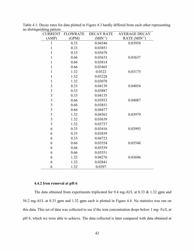
42

Table 4.1: Decay rates for data plotted in Figure 4.3 hardly differed from each other representing no distinguishing pattern

CURRENT (AMP)

FLOWRATE (GPM)

DECAY RATE (MIN-1)

AVERAGE DECAY RATE (MIN-1)

1 0.33 0.04346 0.03958 1 0.33 0.03851 1 0.33 0.03678 1 0.66 0.03633 0.03637 1 0.66 0.03814 1 0.66 0.03465 1 1.32 0.0322 0.03175 1 1.32 0.03228 1 1.32 0.03078 3 0.33 0.04139 0.04054 3 0.33 0.03887 3 0.33 0.04135 3 0.66 0.03933 0.04087 3 0.66 0.03851 3 0.66 0.04477 3 1.32 0.04562 0.03979 3 1.32 0.03639 3 1.32 0.03737 6 0.33 0.03416 0.03993 6 0.33 0.03839 6 0.33 0.04723 6 0.66 0.03554 0.03548 6 0.66 0.03539 6 0.66 0.03551 6 1.32 0.04276 0.03696

6 1.32 0.02841 6 1.32 0.0397

4.4.2 Iron removal at pH 6

The data obtained from experiments triplicated for 9.4 mg-Al/L at 0.33 & 1.32 gpm and

56.2 mg-Al/L at 0.33 gpm and 1.32 gpm each is plotted in Figure 4.4. No statistics was run on

this data. This set of data was collected to see if the iron concentration drops below 1 mg- Fe/L at

pH 6, which we were able to achieve. The data collected is later compared with data obtained at

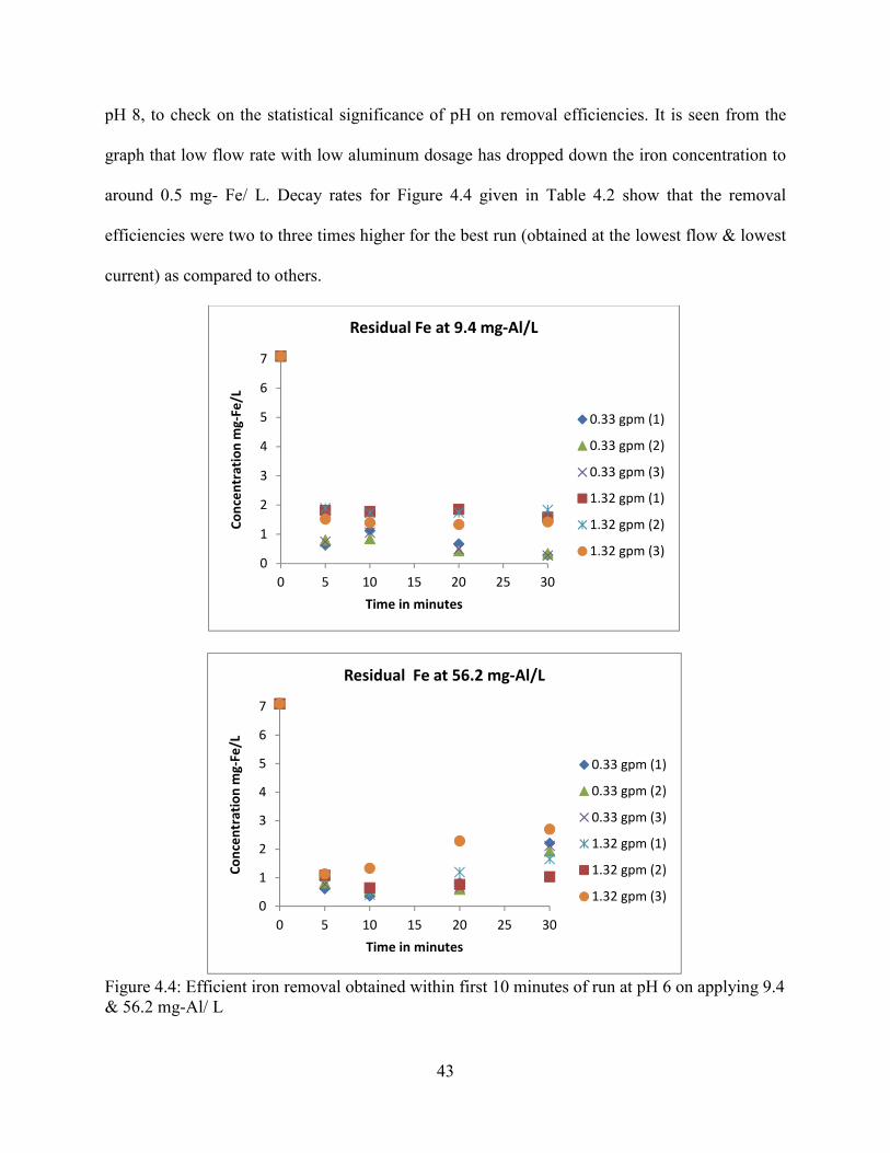
43

pH 8, to check on the statistical significance of pH on removal efficiencies. It is seen from the

graph that low flow rate with low aluminum dosage has dropped down the iron concentration to

around 0.5 mg- Fe/ L. Decay rates for Figure 4.4 given in Table 4.2 show that the removal

efficiencies were two to three times higher for the best run (obtained at the lowest flow & lowest

current) as compared to others.

Figure 4.4: Efficient iron removal obtained within first 10 minutes of run at pH 6 on applying 9.4 & 56.2 mg-Al/ L

0

1

2

3

4

5

6

7

0 5 10 15 20 25 30

Co

nce

ntr

atio

n m

g-Fe

/L

Time in minutes

Residual Fe at 9.4 mg-Al/L

0.33 gpm (1)

0.33 gpm (2)

0.33 gpm (3)

1.32 gpm (1)

1.32 gpm (2)

1.32 gpm (3)

0

1

2

3

4

5

6

7

0 5 10 15 20 25 30

Co

nce

ntr

atio

n m

g-Fe

/L

Time in minutes

Residual Fe at 56.2 mg-Al/L

0.33 gpm (1)

0.33 gpm (2)

0.33 gpm (3)

1.32 gpm (1)

1.32 gpm (2)

1.32 gpm (3)

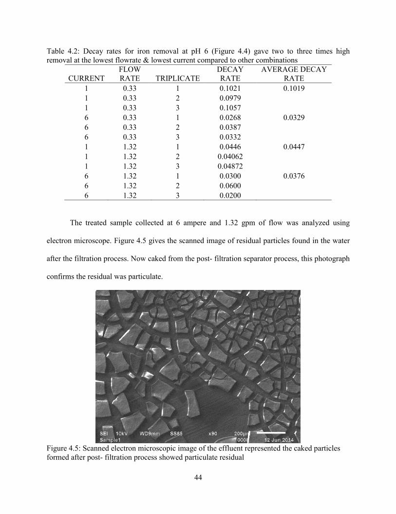
44

Table 4.2: Decay rates for iron removal at pH 6 (Figure 4.4) gave two to three times high removal at the lowest flowrate & lowest current compared to other combinations

CURRENT FLOW RATE TRIPLICATE

DECAY RATE

AVERAGE DECAY RATE

1 0.33 1 0.1021 0.1019 1 0.33 2 0.0979 1 0.33 3 0.1057 6 0.33 1 0.0268 0.0329 6 0.33 2 0.0387 6 0.33 3 0.0332 1 1.32 1 0.0446 0.0447 1 1.32 2 0.04062 1 1.32 3 0.04872 6 1.32 1 0.0300 0.0376 6 1.32 2 0.0600 6 1.32 3 0.0200

The treated sample collected at 6 ampere and 1.32 gpm of flow was analyzed using

electron microscope. Figure 4.5 gives the scanned image of residual particles found in the water

after the filtration process. Now caked from the post- filtration separator process, this photograph

confirms the residual was particulate.

Figure 4.5: Scanned electron microscopic image of the effluent represented the caked particles formed after post- filtration process showed particulate residual

45

Table 4.3 gives the distribution of three elements of concern in the sample scanned by

SEM. Initial amount of iron added was 7.1 mg-Fe/ L and aluminum added was 56.2 mg-Al/ L.

Table 4.3: Distribution by weight of oxygen, aluminum and iron in water sample analyzed by SEM observed that enough aluminum was present for coagulation of iron

ELEMENT PERCENT WEIGHT

O 52.06

Al 44.17

Fe 1.81

Values shown in Table 4.1, are consistent with the theory that the residual particles are iron and

aluminum hydroxides.

4.4.3 Comparison of removals obtained at pH 8 and 6

The iron removal efficiencies obtained at the two pHs are highly different. Figure 4.6

show the iron removal obtained at pH 8 and 6 when currents applied were 9.4 and 56.2 mg-Al/

L. It was also proved statistically that the pH has significant effect on the removal efficiencies.

Rather, all the parameters have p- values less than 0.05, thus, showing significant effect on the

iron removal. The graphs plotted show exponential decay curves. Hence, decay rates were first

obtained by taking log of concentrations against time. Analysis of variance was then run on these

decay rates. The best run obtained at lowest flow, lowest current and pH 6 showed 2.5 times

better iron removal than the lowest combinations of current & flow run at pH 8, as concluded

from Tables 4.1 & 4.2.

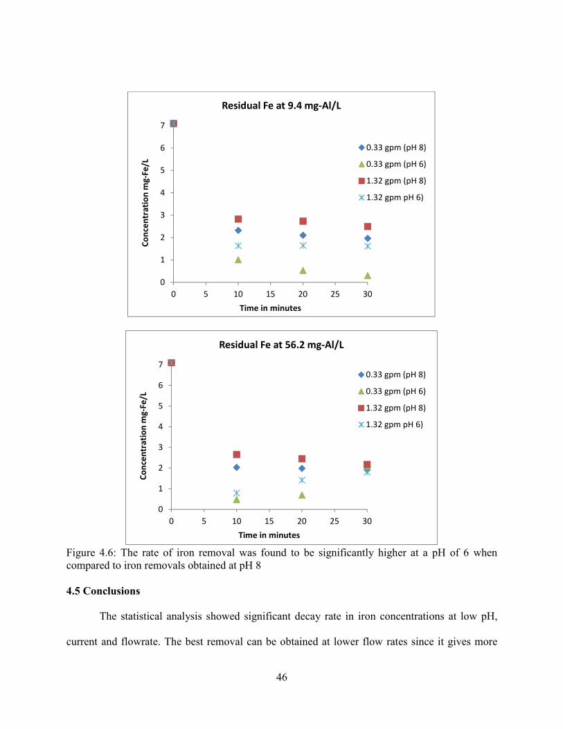
46

Figure 4.6: The rate of iron removal was found to be significantly higher at a pH of 6 when compared to iron removals obtained at pH 8

4.5 Conclusions

The statistical analysis showed significant decay rate in iron concentrations at low pH,

current and flowrate. The best removal can be obtained at lower flow rates since it gives more

0

1

2

3

4

5

6

7

0 5 10 15 20 25 30

Co

nce

ntr

atio

n m

g-Fe

/L

Time in minutes

Residual Fe at 9.4 mg-Al/L

0.33 gpm (pH 8)

0.33 gpm (pH 6)

1.32 gpm (pH 8)

1.32 gpm pH 6)

0

1

2

3

4

5

6

7

0 5 10 15 20 25 30

Co

nce

ntr

atio

n m

g-Fe

/L

Time in minutes

Residual Fe at 56.2 mg-Al/L

0.33 gpm (pH 8)

0.33 gpm (pH 6)

1.32 gpm (pH 8)

1.32 gpm pH 6)

47

retention in the coagulation basin. This helps in proper floc formation. High flow are causing

breakthrough in the bead bed resulting in increase of iron concentrations in the effluent.

Breakthrough phenomenon was not prominent in the preliminary high flow runs but the iron

concentrations never dropped as low as they did at pH 6. Lack of initial clustering of

contaminant particles restricted their removal by the bead bed. The preliminary runs carried out

at pH 8 could not lower the iron concentration lesser than 1.5- 2 mg-Fe/ L. It can also be seen

that the iron concentrations for few of the preliminary runs at 20 and 30 min are nearly same. If

sampling was done for next 5 to 10 minutes, they may have shown an increase because of

breakthrough. The agglomeration of flocs formed can be promoted by adding flocculating basins

between the coagulation tank and the filter column. This would also give enough retention time

for flocculation. pH made a big difference in the removal achieved. The initial assumption that

the pH will not affect the process to a great extent was wrong. The electrocoagulation process

using aluminum electrodes for iron removal works best at low pH. Proper range of pH (6±0.2),

aluminum coagulant (≈ 9 mg-Al/ L), flow rate (< 0.4 gpm) achieved the goal of this chapter of

dropping down the iron concentrations below 0.3 mg-Fe/L.

48

CHAPTER 5: IRON REMOVAL EFFICIENCY OF IRON PRECOATED FLOATING BEAD BED BY APPLICATION OF ELECTROCOAGULATION

5.1 Introduction

Iron, is an essential dietary supplement and should be included in certain amounts in diet.

Thus, EPA records iron as a secondary contaminant since its presence is not harmful but can

cause problems like staining, pipe fouling, taste issues, color problems and stock losses in

aquaculture. Permissible secondary contaminant level for iron is 0.3 mg-Fe/ L as set by EPA.

Many Louisiana aquifer systems have iron concentrations higher than this permitted amount.

Adsorption- oxidation mechanism involves the removal of ferrous iron from water by

adsorption to media followed by its oxidation to ferric. Iron coated media is known improve iron

removal by adsorbing more contaminant iron. The adsorbed iron causes an increase in the

surface area of the media particles. Larger surface area of media particles facilitates more

contaminant removal since adsorption is directly proportional to surface area of the media. This

method is cheap and hence can be employed to purify water in rural areas where there is a need

for using cost effective technologies and where time is not the constraint.

Electrocoagulation can be used in combination with filtration to remove iron. Application

of an electrical current to a sacrificial anode generates the coagulant ions required for particle

destabilization thus facilitating flocculation. The flocs formed can then be filtered by using

proper filtration media generally providing high surface area. Polyethylene floating beds with 2-

3 mm beads have surface area ranging from 1050- 1300 m2/ m3 (Ahmed, 1996). The objective of

this chapter was to develop iron coating around these polyethylene floating beads and to check if

the iron removal efficiency of these beads is higher than the fresh beads on applying

electrocoagulation prior to filtration through the bead bed.

49

5.2 Background

Sharma, 2001 has demonstrated the adsorption technique using various media like sand,

basalt, anthracite, limestone, iron coated sand and others. He tested the adsorption capacities of

various media over a pH range of 6 to 7.5 and found iron coated sand to work better than the

fresh sand. The iron coating formed on the sand grains due to adsorption increase its specific

surface area thus, attributing to higher adsorptive removal. Adsorption of iron occurs when the

iron in solution is in ferrous state which first, gets adsorbed to the media particles and is then

oxidized to ferric coating around the media. Amount of material adsorbed on the solid surface

can be given as the materials adsorption density in mg/ m2.

Adsorption can occur as a result of two forces of attraction, resulting in; physical

adsorption (Van der Waals’ forces) or chemical adsorption (chemical bonds). Media particles get

charged when they come in contact with a moving fluid. The charged surfaces attract the metal

ions to be removed. Also, surface charge of adsorbing surface plays a vital role. If the surface

carries a negative charge then they can easily attract positive ions. Examples of some solids used

as adsorbents are activated carbon, ion exchange resins and oxides of aluminum and iron.

Efficiency of adsorption process is dictated by factors including pH, dissolved oxygen, surface

area of the media and its surface charge. The process can be used for removing inorganically &

organically complexed metals over various pH settings if the chemistry of solution is properly set

for specific adsorbent surfaces (Benjamin et al., 1996).

5.3 Materials and methods

5.3.1 Experimental coating

First objective of this paper was to form iron coating around polyethylene plastic beads.

A plastic container used to coat the beads is shown in Figure 5.1. This container was placed on

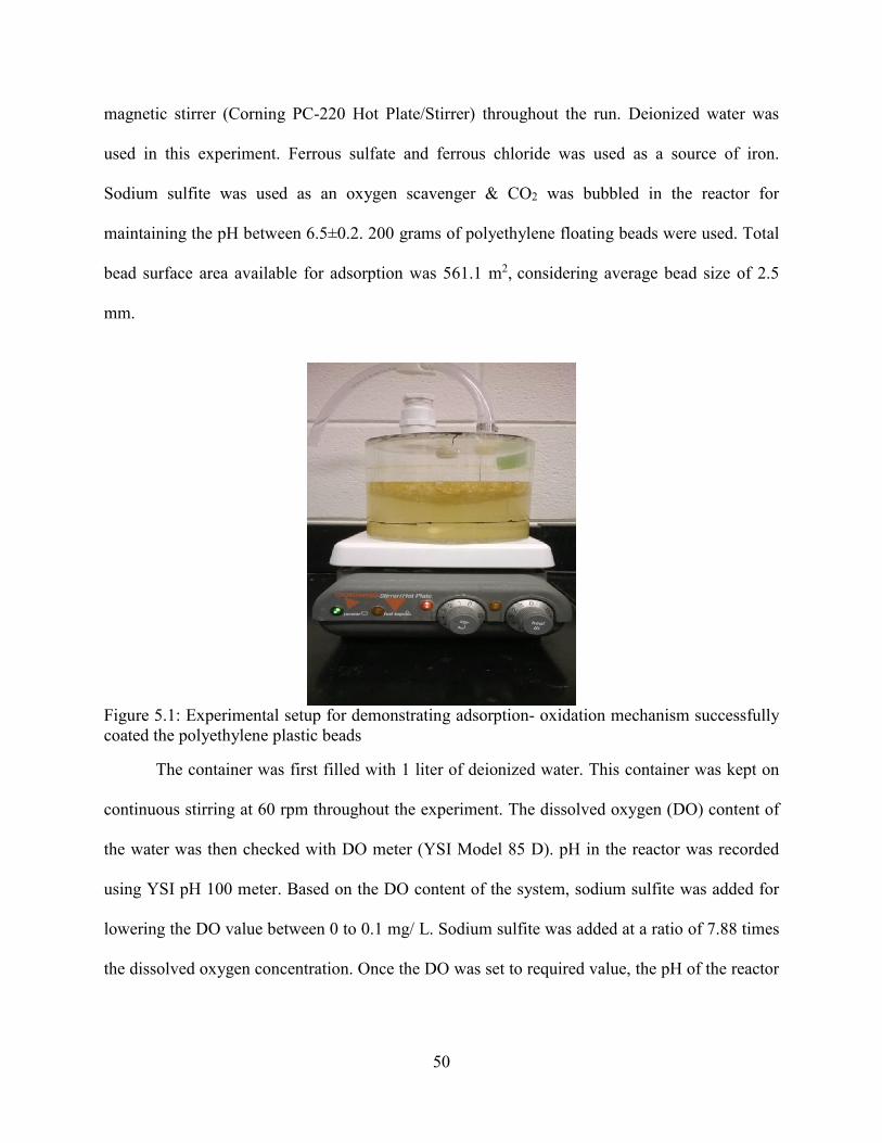
50

magnetic stirrer (Corning PC-220 Hot Plate/Stirrer) throughout the run. Deionized water was

used in this experiment. Ferrous sulfate and ferrous chloride was used as a source of iron.

Sodium sulfite was used as an oxygen scavenger & CO2 was bubbled in the reactor for

maintaining the pH between 6.5±0.2. 200 grams of polyethylene floating beads were used. Total

bead surface area available for adsorption was 561.1 m2, considering average bead size of 2.5

mm.

Figure 5.1: Experimental setup for demonstrating adsorption- oxidation mechanism successfully coated the polyethylene plastic beads

The container was first filled with 1 liter of deionized water. This container was kept on

continuous stirring at 60 rpm throughout the experiment. The dissolved oxygen (DO) content of

the water was then checked with DO meter (YSI Model 85 D). pH in the reactor was recorded

using YSI pH 100 meter. Based on the DO content of the system, sodium sulfite was added for

lowering the DO value between 0 to 0.1 mg/ L. Sodium sulfite was added at a ratio of 7.88 times

the dissolved oxygen concentration. Once the DO was set to required value, the pH of the reactor

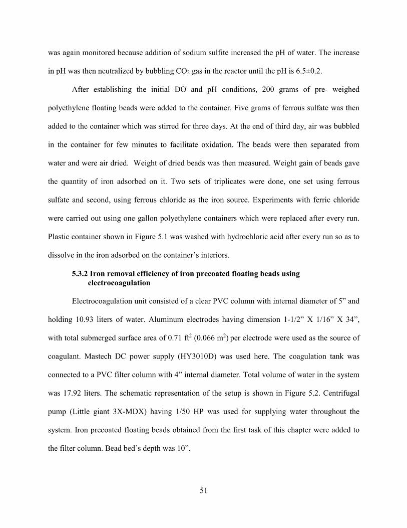
51

was again monitored because addition of sodium sulfite increased the pH of water. The increase

in pH was then neutralized by bubbling CO2 gas in the reactor until the pH is 6.5±0.2.

After establishing the initial DO and pH conditions, 200 grams of pre- weighed

polyethylene floating beads were added to the container. Five grams of ferrous sulfate was then

added to the container which was stirred for three days. At the end of third day, air was bubbled

in the container for few minutes to facilitate oxidation. The beads were then separated from

water and were air dried. Weight of dried beads was then measured. Weight gain of beads gave

the quantity of iron adsorbed on it. Two sets of triplicates were done, one set using ferrous

sulfate and second, using ferrous chloride as the iron source. Experiments with ferric chloride

were carried out using one gallon polyethylene containers which were replaced after every run.

Plastic container shown in Figure 5.1 was washed with hydrochloric acid after every run so as to

dissolve in the iron adsorbed on the container’s interiors.

5.3.2 Iron removal efficiency of iron precoated floating beads using electrocoagulation

Electrocoagulation unit consisted of a clear PVC column with internal diameter of 5” and

holding 10.93 liters of water. Aluminum electrodes having dimension 1-1/2” X 1/16” X 34”,

with total submerged surface area of 0.71 ft2 (0.066 m2) per electrode were used as the source of

coagulant. Mastech DC power supply (HY3010D) was used here. The coagulation tank was

connected to a PVC filter column with 4” internal diameter. Total volume of water in the system

was 17.92 liters. The schematic representation of the setup is shown in Figure 5.2. Centrifugal

pump (Little giant 3X-MDX) having 1/50 HP was used for supplying water throughout the

system. Iron precoated floating beads obtained from the first task of this chapter were added to

the filter column. Bead bed’s depth was 10”.

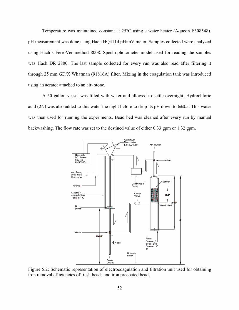
52

Temperature was maintained constant at 25°C using a water heater (Aqueon E308548).

pH measurement was done using Hach HQ411d pH/mV meter. Samples collected were analyzed

using Hach’s FerroVer method 8008. Spectrophotometer model used for reading the samples

was Hach DR 2800. The last sample collected for every run was also read after filtering it

through 25 mm GD/X Whatman (91816A) filter. Mixing in the coagulation tank was introduced

using an aerator attached to an air- stone.

A 50 gallon vessel was filled with water and allowed to settle overnight. Hydrochloric

acid (2N) was also added to this water the night before to drop its pH down to 6±0.5. This water

was then used for running the experiments. Bead bed was cleaned after every run by manual

backwashing. The flow rate was set to the destined value of either 0.33 gpm or 1.32 gpm.

Figure 5.2: Schematic representation of electrocoagulation and filtration unit used for obtaining iron removal efficiencies of fresh beads and iron precoated beads

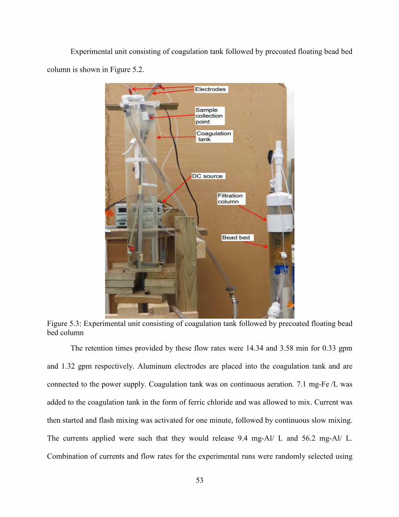
53

Experimental unit consisting of coagulation tank followed by precoated floating bead bed

column is shown in Figure 5.2.

Figure 5.3: Experimental unit consisting of coagulation tank followed by precoated floating bead bed column

The retention times provided by these flow rates were 14.34 and 3.58 min for 0.33 gpm

and 1.32 gpm respectively. Aluminum electrodes are placed into the coagulation tank and are

connected to the power supply. Coagulation tank was on continuous aeration. 7.1 mg-Fe /L was

added to the coagulation tank in the form of ferric chloride and was allowed to mix. Current was

then started and flash mixing was activated for one minute, followed by continuous slow mixing.

The currents applied were such that they would release 9.4 mg-Al/ L and 56.2 mg-Al/ L.

Combination of currents and flow rates for the experimental runs were randomly selected using

54

ExcelTM random number generator. The experiments were run for 30 minutes. Sampling done for

every 10 min was analyzed by following Hach’s FerroVer method 8008. Iron concentration vs

time was then plotted. The system was cleaned by draining and manual backflushing after every

run. Polarity of electrodes was changed for every run. The electrodes were scrubbed using sand

paper and later washed with acetone after every six runs to remove the depositions from

electrode plates.

5.4 Results and discussion

5.4.1 Experimental coating

These experiments were run only for a limited period of time, until a visible coating was

observed. Prolonged exposure of the beads to high iron contents will result in dense iron

coatings. Triplicated data represented weight gain of 5.93 * 10-5 mg/cm2 and 7.71 * 10-5 mg/cm2,

after three days dosed with ferrous sulfate and ferrous chloride, respectively. Higher pH with

presence of oxygen did not show any coating because of immediate conversion of ferrous to

ferric precipitate. Lack of negative surface charge on beads makes iron adsorption on beads a

slow process as compared to its adsorption on sand surface which has a negative surface charge.

Coated bead media may adsorb more iron as sand media but thicker coatings will eventually

result in the sinking of these beads due to increase in the specific gravity of beads making them

heavier than water.

Maintaining proper pH is very important in this experiment. Initial study was done by

circulating iron contaminated water through a floating bead bed. The dissolved oxygen content in

this system was lowered down to zero but the pH was not monitored. No coat formation on the

bead media was observed. The experiment was thus rerun by replacing bead media with sand.

Sand media formed coating for the same conditions of dissolved oxygen and pH. Deionized

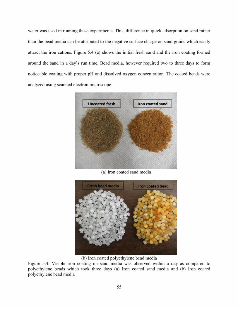
55

water was used in running these experiments. This, difference in quick adsorption on sand rather

than the bead media can be attributed to the negative surface charge on sand grains which easily

attract the iron cations. Figure 5.4 (a) shows the initial fresh sand and the iron coating formed

around the sand in a day’s run time. Bead media, however required two to three days to form

noticeable coating with proper pH and dissolved oxygen concentration. The coated beads were

analyzed using scanned electron microscope.

(a) Iron coated sand media

(b) Iron coated polyethylene bead media

Figure 5.4: Visible iron coating on sand media was observed within a day as compared to polyethylene beads which took three days (a) Iron coated sand media and (b) Iron coated polyethylene bead media

Uncoated fresh Iron coated sand

Fresh bead media Iron coated bead

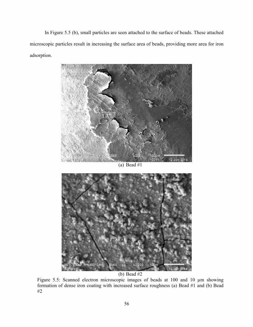
56

In Figure 5.5 (b), small particles are seen attached to the surface of beads. These attached

microscopic particles result in increasing the surface area of beads, providing more area for iron

adsorption.

(a) Bead #1

(b) Bead #2

Figure 5.5: Scanned electron microscopic images of beads at 100 and 10 µm showing formation of dense iron coating with increased surface roughness (a) Bead #1 and (b) Bead #2

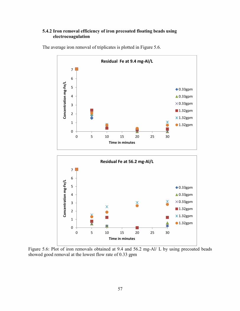
57

5.4.2 Iron removal efficiency of iron precoated floating beads using electrocoagulation The average iron removal of triplicates is plotted in Figure 5.6.

Figure 5.6: Plot of iron removals obtained at 9.4 and 56.2 mg-Al/ L by using precoated beads showed good removal at the lowest flow rate of 0.33 gpm

0

1

2

3

4

5

6

7

0 5 10 15 20 25 30

Co

nce

ntr

atio

n m

g-Fe

/L

Time in minutes

Residual Fe at 9.4 mg-Al/L

0.33gpm

0.33gpm

0.33gpm

1.32gpm

1.32gpm

1.32gpm

0

1

2

3

4

5

6

7

0 5 10 15 20 25 30

Co

nce

ntr

atio

n m

g-Fe

/L

Time in minutes

Residual Fe at 56.2 mg-Al/L

0.33gpm

0.33gpm

0.33gpm

1.32gpm

1.32gpm

1.32gpm

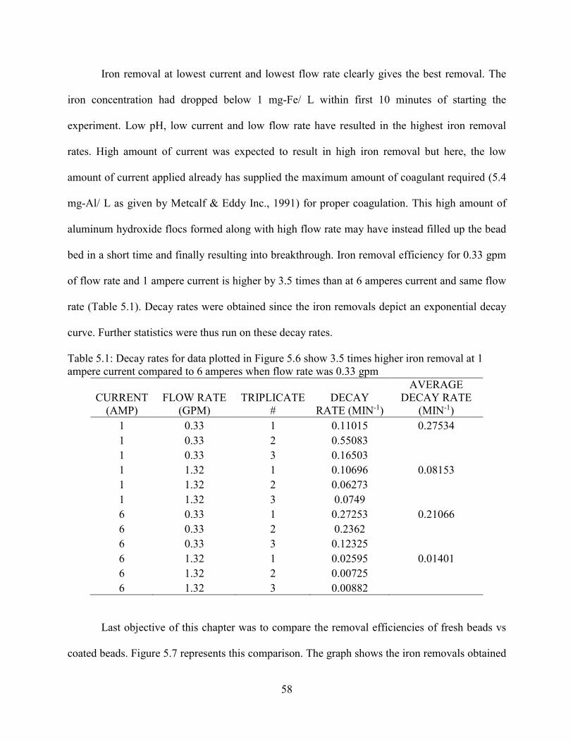
58

Iron removal at lowest current and lowest flow rate clearly gives the best removal. The

iron concentration had dropped below 1 mg-Fe/ L within first 10 minutes of starting the

experiment. Low pH, low current and low flow rate have resulted in the highest iron removal

rates. High amount of current was expected to result in high iron removal but here, the low

amount of current applied already has supplied the maximum amount of coagulant required (5.4

mg-Al/ L as given by Metcalf & Eddy Inc., 1991) for proper coagulation. This high amount of

aluminum hydroxide flocs formed along with high flow rate may have instead filled up the bead

bed in a short time and finally resulting into breakthrough. Iron removal efficiency for 0.33 gpm

of flow rate and 1 ampere current is higher by 3.5 times than at 6 amperes current and same flow

rate (Table 5.1). Decay rates were obtained since the iron removals depict an exponential decay

curve. Further statistics were thus run on these decay rates.

Table 5.1: Decay rates for data plotted in Figure 5.6 show 3.5 times higher iron removal at 1 ampere current compared to 6 amperes when flow rate was 0.33 gpm

CURRENT (AMP)

FLOW RATE (GPM)

TRIPLICATE #

DECAY RATE (MIN-1)

AVERAGE DECAY RATE

(MIN-1)

1 0.33 1 0.11015 0.27534

1 0.33 2 0.55083

1 0.33 3 0.16503

1 1.32 1 0.10696 0.08153

1 1.32 2 0.06273

1 1.32 3 0.0749

6 0.33 1 0.27253 0.21066

6 0.33 2 0.2362

6 0.33 3 0.12325

6 1.32 1 0.02595 0.01401

6 1.32 2 0.00725

6 1.32 3 0.00882

Last objective of this chapter was to compare the removal efficiencies of fresh beads vs

coated beads. Figure 5.7 represents this comparison. The graph shows the iron removals obtained

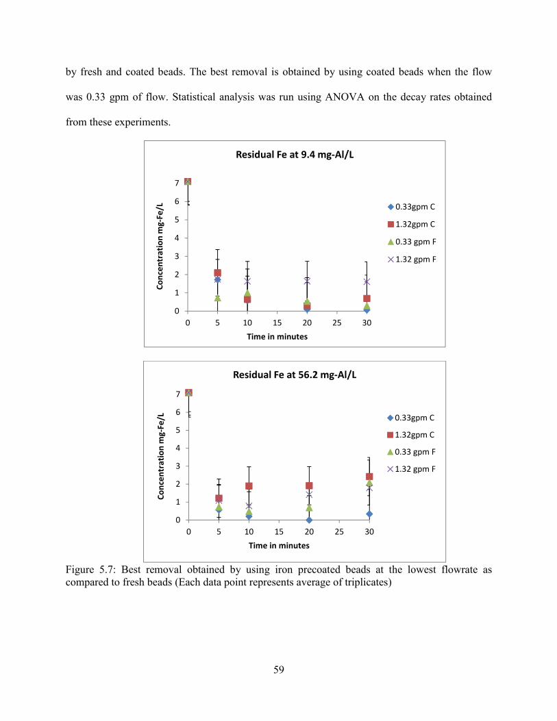
59

by fresh and coated beads. The best removal is obtained by using coated beads when the flow

was 0.33 gpm of flow. Statistical analysis was run using ANOVA on the decay rates obtained

from these experiments.

Figure 5.7: Best removal obtained by using iron precoated beads at the lowest flowrate as compared to fresh beads (Each data point represents average of triplicates)

0

1

2

3

4

5

6

7

0 5 10 15 20 25 30

Co

nce

ntr

atio

n m

g-Fe

/L

Time in minutes

Residual Fe at 9.4 mg-Al/L

0.33gpm C

1.32gpm C

0.33 gpm F

1.32 gpm F

0

1

2

3

4

5

6

7

0 5 10 15 20 25 30

Co

nce

ntr

atio

n m

g-Fe

/L

Time in minutes

Residual Fe at 56.2 mg-Al/L

0.33gpm C

1.32gpm C

0.33 gpm F

1.32 gpm F

60

The effect of bead type was highly significant. Further statistical tests showed that the

coated beads promoted more iron removal since the decay rate estimated for these was higher

than that of fresh beads by 3.5 times (see Appendix A).

5.5 Conclusions

Procedure of bead coating requires specific system conditions to work. Low pH

i.e. < 3 result in having all the ferrous iron dissolved in solution. It won’t adsorb on the bead

surface. Whereas, higher pH results in immediate precipitation of iron. It is important to maintain

the pH of water between 6.5±0.2 for observing any coating around beads. These beads do not

have any negative surface charge and hence do not promote fast adsorption of positive ferrous

ions unlike sand. Effect of sodium sulfite used for scavenging out the oxygen from the system on

the coat formation needs to be evaluated. This coating problem may be observed for floating

bead filters installed for filtering groundwater which many of the times have low pH and anoxic

conditions. Shallow groundwater conditions in Louisiana having pH < 7.0 and low dissolved

oxygen condition can cause such coating on the beads. To avoid the floating bead media from

getting coated with iron, complete oxidation of iron is suggested before the water is passed

through the filtration column.

Removal achieved by using coated beads graphically though looked same as that

achieved by fresh beads, depicted difference statistically. Though the coated sand media is

known to perform better than fresh sand (Sharma, 2001), case is not the same when using

floating beads. As the thickness of coating around the beads increase, so will its specific gravity.

Increase in the specific gravity will cause the beads to sink and will result in failure of the

filtration system.

61

CHAPTER 6: CONCLUSIONS AND RECOMMENDATIONS

Various factors known to affect the electrocoagulation process were current applied, pH

and flowrate. According to Metcalf & Eddy Inc., 1991, maximum amount of aluminum required

to be dosed for coagulation to work best is 5.4 mg-Al/ L, effective pH range for proper

coagulation using aluminum is 5.8 to 9. Current range selected here was already supplying

aluminum dosage higher than 5.4 mg-Al/ L. Thus, no improvement in iron removal could be

seen at higher currents. Applying high currents would result only in wastage of energy and

material. Amount of current to be supplied should hence first calculated using equation 1 from

chapter 2. The value should be selected such that it would release around 5.4 mg-Al/ L.

Experiments carried out in this research showed significant differences in the removal

efficiencies obtained at pH 8 and pH 6. Initial assumption that the pH being selected in proper

range and will not affect the removal process was wrong. Electrocoagulation process being very

complicated, it requires thorough study on how pH made so much of difference and what

compounds are being formed at different pH which helped in the iron removal. It can be

concluded here that iron removal efficiency using aluminum electrodes is higher at low pH.

Dropping the pH below 6 might again start to drop the removal efficiencies since aluminum and

iron are both soluble at lower pH i.e. < 3.

Recirculation flow rate has shown to have prominent effect on the removal efficiencies.

Flow rate set in the system regulated the retention time in the coagulation tank. Low flow rate

provided higher retention in the coagulation basin. This gave enough time required for complete

coagulation and flocculation. If enough time is not provided for flocculation after addition of

coagulant it will result into dispersed flocs which do not get enough time for clustering into

larger particles. Smaller sized flocs were not captured into the bead bed. The particulate iron

62

present must have easily passed through the bead bed. The polyethylene beads used can capture

almost 100% of particles sized > 50 microns (Ahmed, 1990). Low flow rate at higher pH did

result in high removal efficiencies as compared with those obtained at low pH. The combination

of low recirculating flow rate and low pH demonstrated highest iron removal again ascribing to

the complexity of the process. The iron concentration was brought down to about 0.3 mg-Fe/ L

in 30 minutes. High flow rates have resulted in breakthrough of contaminant particles at many

times in the experimentation. Problem of breakthrough can be overcome by timely backwashing

the bead bed.

Coming to bead coating, it is prominent at low pH and minimal dissolved oxygen

concentrations. A pH of 6.5±0.2 demonstrated coat formation on beads. Lower pH did not show

any visible coat formation since most of the ferrous iron stays soluble at low pH. Lack of

negative surface charge on beads was detriment for the bead coating process since it does not

easily attract the iron cations as is applicable for negatively charged sand particles. Particle

accumulation ranging 5.93 * 10-5 mg/ cm2 to 7.71 * 10-5 mg/ cm2 was obtained in three days.

Most groundwater support these low pH and low DO conditions. If this water is passed

through the bead bed for filtration it will result in adsorption of iron on the bead surface. Though

adsorption is one of the filtration techniques, in case of floating bead media it results in increase

in specific gravity of these beads eventually causing failure of filter due to sinking of beads.

Thus, to purify such waters, it is necessary to completely oxidize the ferrous iron before allowing

it pass through the filter bed. Aerating the waters prior to filtration will increase the dissolved

oxygen content, remove the carbon dioxide from water thus, raising its pH and expediting the

oxidation of ferrous iron. Suggested system conditions are summarized in Table 6.1.

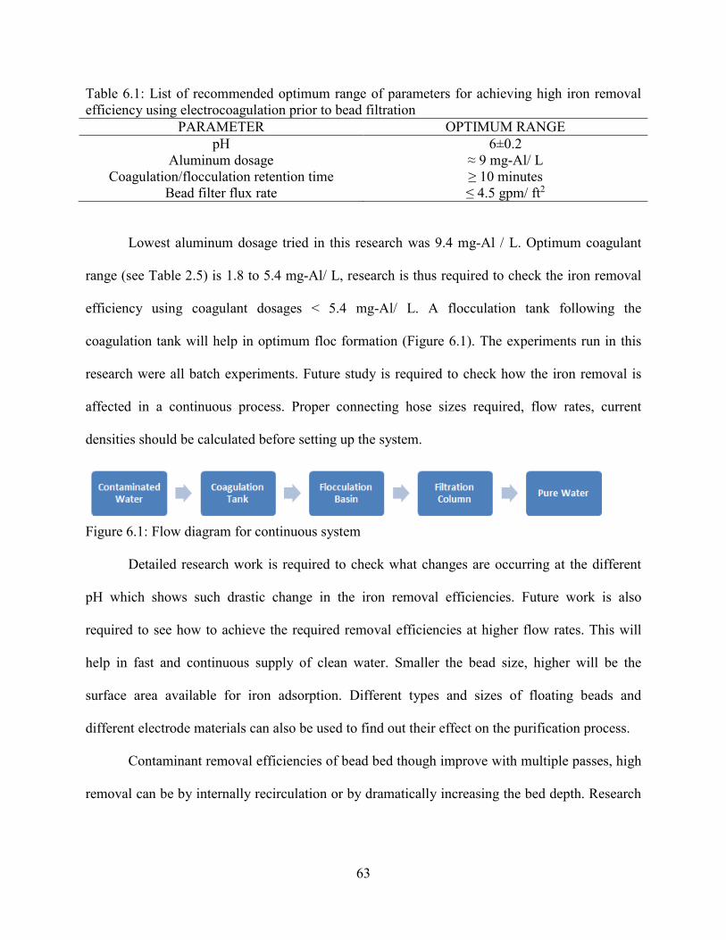
63

Table 6.1: List of recommended optimum range of parameters for achieving high iron removal efficiency using electrocoagulation prior to bead filtration

PARAMETER OPTIMUM RANGE pH 6±0.2

Aluminum dosage ≈ 9 mg-Al/ L Coagulation/flocculation retention time ≥ 10 minutes

Bead filter flux rate ≤ 4.5 gpm/ ft2

Lowest aluminum dosage tried in this research was 9.4 mg-Al / L. Optimum coagulant

range (see Table 2.5) is 1.8 to 5.4 mg-Al/ L, research is thus required to check the iron removal

efficiency using coagulant dosages < 5.4 mg-Al/ L. A flocculation tank following the

coagulation tank will help in optimum floc formation (Figure 6.1). The experiments run in this

research were all batch experiments. Future study is required to check how the iron removal is

affected in a continuous process. Proper connecting hose sizes required, flow rates, current

densities should be calculated before setting up the system.

Figure 6.1: Flow diagram for continuous system

Detailed research work is required to check what changes are occurring at the different

pH which shows such drastic change in the iron removal efficiencies. Future work is also

required to see how to achieve the required removal efficiencies at higher flow rates. This will

help in fast and continuous supply of clean water. Smaller the bead size, higher will be the

surface area available for iron adsorption. Different types and sizes of floating beads and

different electrode materials can also be used to find out their effect on the purification process.

Contaminant removal efficiencies of bead bed though improve with multiple passes, high

removal can be by internally recirculation or by dramatically increasing the bed depth. Research

64

is required here to determine the relationships between removal efficiency and the controlling

variables including bed depth, number of passes, fluxrates, and bead size.

65

REFERENCES

Ahmed, H. U. (1990). “The effects of fluxrate and solids accumulation on small size particle accumulation in expandable granular bead filters.” A thesis, Louisiana State University.

Ankrah, D. A., and Søgaard E. G. (2009). “A review of biological iron removal.”

Thirteenth International Water Technology Conference, IWTC 13, Hurghada, Egypt: 999-1005.

Ayotte, J. D., Gronberg, J. M., and Apodaca, L. E. (2011). “Trace elements and radon in

groundwater across the United States.” U.S. Geological Survey Scientific Investigations Report 5059, 115 p.

Benjamin, M. M., and Lawler, D. F. (2013). “Water quality engineering: physical/ chemical

treatment processes.” John Wiley & Sons, Inc. Benjamin, M. M., Sletten, R. S., Bailey, R. P., and Bennett, T. (1996). “Sorption and filtration of

metals using iron-oxide-coated sand.” War. Res. 30(11): 2609-2620.

Buttner, J. K., Soderberg, R. W., and Terlizzi, D. E. (1993). “An introduction to water chemistry in freshwater aquaculture.” Northeastern Regional Aquaculture Center, 170. Chaturvedi, S., and Dave, P. N. (2012). “Removal of iron for safe drinking water.” Desalination

303: 1–11. Chen, G. (2004). “Electrochemical technologies in wastewater treatment.” Separation and

Purification Technology 38: 11–41. Comninellis, C., and Chen, G. (eds.) (2010). “Electrochemistry for the Environment”,

DOI 10.1007/978-0-387-68318-810, Springer Science+Business Media, LLC: 245-262. Conte, F. S. (1993). “Evaluation of a freshwater site for aquaculture potential”, Western

Regional Aquaculture Center, WRAC Publication No. 92-101. EC-Official Journal of the European Communities Council Directive. (1998). 98/83/EC L

330/32. EPA. (1995). “Water treatment manuals- filtration”. Ardcavan, Wexford, Ireland. EPA. (2013). “Secondary drinking water regulations: guidance for nuisance chemicals”, United

States Environmental Protection Agency. Garbarino, J. R., Hayes, H. C., Roth, D. A., Antweiler, R. C., Brinton, T. I., and Taylor, H. E.

(1995). “Heavy metals in the Mississippi river (contaminants in the Mississippi river).” U.S. Geological Survey Circular 1133.

66

General Electrical Company. (2012). “Chapter 08- ion exchange, water and process

technologies.” c1997-2012. Ghosh, D., Solanki, H., and Purkait, M. K. (2008). “Removal of Fe(II) from tap water by

electrocoagulation technique.” Journal of Hazardous Materials 155: 135–143. Harland, C. E. (1994). “Ion exchange: theory and practice.” Royal Society of Chemistry. Harmon, S. (2003). “A complete guide to iron removal methods, iron conditioning equipment

and their limitations.” Water Technology magazine. Iron removal systems, copyright JP Anderson 2013.

Holmden, B. (2013). “Drinking water C & D certification review.” Florida Rural Water

Association. ITRC (Interstate Technology & Regulatory Council). (2010). “Electrocoagulation.” Washington,

D.C.: Interstate Technology & Regulatory Council, Mining Waste Team. (www.itrcweb.org)

Ityel, D. (2011). “Ground water: dealing with iron contamination.” Filtration and Separation

48(1): 26-28. Kenny, J. F., Barber, N. L., Hutson, S. S., Linsey, K. S., Lovelace, J. K., and Maupin, M. A.

(2009). Estimated use of water in the United States in 2005: U.S. Geological Survey Circular 1344, 52 p.

Mollah, M. Y. A., Morkovsky, P., Gomes, J. A. G., Kesmezc, M., Parga, J., and Cocke, D. L.

(2004). “Fundamentals, present and future perspectives of electrocoagulation.” Journal of Hazardous Materials B114: 199–210.

National ground water association. (2010). “Groundwater facts.”

(http://www.ngwa.org/fundamentals/use/pages/groundwater-facts.aspx). National Water Summary. (1986), “Groundwater Quality: Louisiana.” 273-278. Robinson, R. B., Reed, G. D., Christodos, D., Frazier, B., and Chidambariah, V. (1990).

“Sequestering methods of iron and manganese treatment.” AWWA Research Foundation and American Water Works Association.

Sahu, O., Mazumdar, B., and Chaudhari, P. K. (2014). “Treatment of wastewater by

electrocoagulation: a review” Environ Sci Pollut Res 21: 2397–2413 DOI 10.1007/s11356-013-2208-6

Seelig, B., Derickson, R., and Bergsrud, F. (2013). “Treatment systems for household water

supplies: iron and manganese removal.” Regents of the University of Minnesota.

67

Sharma, S. K. (2001). “Adsorptive iron removal from groundwater.” Dissertation, Academic

Board of Wageningen University and the Academic Board of the Intemational Institute for Infrastructural, Hydraulic and Environmental Engineering.

Silver, J. (1993). “Chemistry of Iron.” Blackie Academic and Professional/Chapman & Hall,

London. Taylor, C., Yahner, J., Jones, D., and Dunn, A. (1997). Indiana State Department of Health,

Pipeline 8(3). Tekerlekopoulou, A. G., Vasiliadou, I. A., and Vayenas, D. V. (2006). “Physico-chemical and

biological iron removal from potable water.” Biochemical Engineering Journal 31: 74–83.

Teunissen, K., Abrahamse, A., Leijssen, H., Rietveld, L., and van Dijk, H. (2008). “Removal of

both dissolved and particulate iron from groundwater.” Drinking Water Engineering and Science Discussions 1: 87–115.

Vance, D. B. (1994). “Iron- the environmental impact of a universal element.” National

Environmental Journal 4(3): 24-25. Wang, L. K., Shammas, N. K., Selke, W. A., and Aulenbach, D. B. (2010). “Flotation

technology.” Handbook of Environmental Engineering 12: 199-220. Springer Science+Business Media, LLC. DOI: 10.1007/978-1-60327-133-26

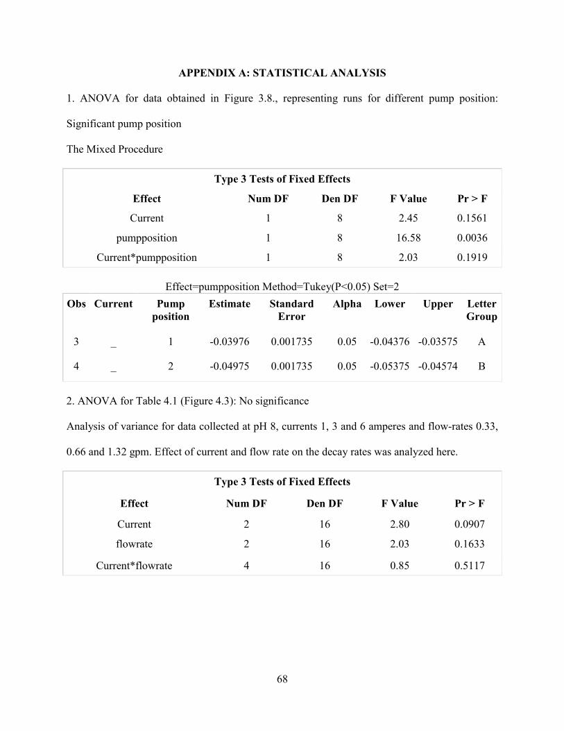
68

APPENDIX A: STATISTICAL ANALYSIS

1. ANOVA for data obtained in Figure 3.8., representing runs for different pump position:

Significant pump position

The Mixed Procedure

Type 3 Tests of Fixed Effects

Effect Num DF Den DF F Value Pr > F

Current 1 8 2.45 0.1561

pumpposition 1 8 16.58 0.0036

Current*pumpposition 1 8 2.03 0.1919

Effect=pumpposition Method=Tukey(P<0.05) Set=2

Obs Current Pump position

Estimate Standard Error

Alpha Lower Upper Letter Group

3 _ 1 -0.03976 0.001735 0.05 -0.04376 -0.03575 A

4 _ 2 -0.04975 0.001735 0.05 -0.05375 -0.04574 B

2. ANOVA for Table 4.1 (Figure 4.3): No significance

Analysis of variance for data collected at pH 8, currents 1, 3 and 6 amperes and flow-rates 0.33,

0.66 and 1.32 gpm. Effect of current and flow rate on the decay rates was analyzed here.

Type 3 Tests of Fixed Effects

Effect Num DF Den DF F Value Pr > F

Current 2 16 2.80 0.0907

flowrate 2 16 2.03 0.1633

Current*flowrate 4 16 0.85 0.5117

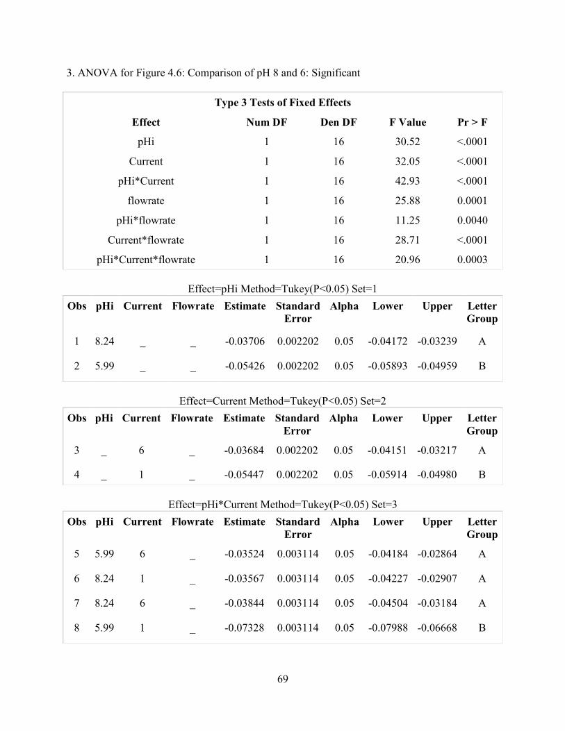
69

3. ANOVA for Figure 4.6: Comparison of pH 8 and 6: Significant

Type 3 Tests of Fixed Effects

Effect Num DF Den DF F Value Pr > F

pHi 1 16 30.52 <.0001

Current 1 16 32.05 <.0001

pHi*Current 1 16 42.93 <.0001

flowrate 1 16 25.88 0.0001

pHi*flowrate 1 16 11.25 0.0040

Current*flowrate 1 16 28.71 <.0001

pHi*Current*flowrate 1 16 20.96 0.0003

Effect=pHi Method=Tukey(P<0.05) Set=1

Obs pHi Current Flowrate Estimate Standard Error

Alpha Lower Upper Letter Group

1 8.24 _ _ -0.03706 0.002202 0.05 -0.04172 -0.03239 A

2 5.99 _ _ -0.05426 0.002202 0.05 -0.05893 -0.04959 B

Effect=Current Method=Tukey(P<0.05) Set=2

Obs pHi Current Flowrate Estimate Standard Error

Alpha Lower Upper Letter Group

3 _ 6 _ -0.03684 0.002202 0.05 -0.04151 -0.03217 A

4 _ 1 _ -0.05447 0.002202 0.05 -0.05914 -0.04980 B

Effect=pHi*Current Method=Tukey(P<0.05) Set=3

Obs pHi Current Flowrate Estimate Standard Error

Alpha Lower Upper Letter Group

5 5.99 6 _ -0.03524 0.003114 0.05 -0.04184 -0.02864 A

6 8.24 1 _ -0.03567 0.003114 0.05 -0.04227 -0.02907 A

7 8.24 6 _ -0.03844 0.003114 0.05 -0.04504 -0.03184 A

8 5.99 1 _ -0.07328 0.003114 0.05 -0.07988 -0.06668 B

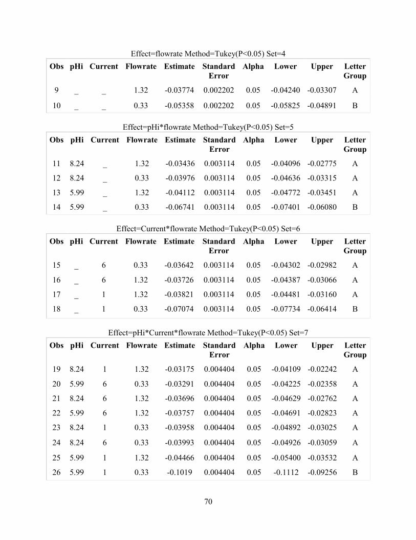
70

Effect=flowrate Method=Tukey(P<0.05) Set=4

Obs pHi Current Flowrate Estimate Standard Error

Alpha Lower Upper Letter Group

9 _ _ 1.32 -0.03774 0.002202 0.05 -0.04240 -0.03307 A

10 _ _ 0.33 -0.05358 0.002202 0.05 -0.05825 -0.04891 B

Effect=pHi*flowrate Method=Tukey(P<0.05) Set=5

Obs pHi Current Flowrate Estimate Standard Error

Alpha Lower Upper Letter Group

11 8.24 _ 1.32 -0.03436 0.003114 0.05 -0.04096 -0.02775 A

12 8.24 _ 0.33 -0.03976 0.003114 0.05 -0.04636 -0.03315 A

13 5.99 _ 1.32 -0.04112 0.003114 0.05 -0.04772 -0.03451 A

14 5.99 _ 0.33 -0.06741 0.003114 0.05 -0.07401 -0.06080 B

Effect=Current*flowrate Method=Tukey(P<0.05) Set=6

Obs pHi Current Flowrate Estimate Standard Error

Alpha Lower Upper Letter Group

15 _ 6 0.33 -0.03642 0.003114 0.05 -0.04302 -0.02982 A

16 _ 6 1.32 -0.03726 0.003114 0.05 -0.04387 -0.03066 A

17 _ 1 1.32 -0.03821 0.003114 0.05 -0.04481 -0.03160 A

18 _ 1 0.33 -0.07074 0.003114 0.05 -0.07734 -0.06414 B

Effect=pHi*Current*flowrate Method=Tukey(P<0.05) Set=7

Obs pHi Current Flowrate Estimate Standard Error

Alpha Lower Upper Letter Group

19 8.24 1 1.32 -0.03175 0.004404 0.05 -0.04109 -0.02242 A

20 5.99 6 0.33 -0.03291 0.004404 0.05 -0.04225 -0.02358 A

21 8.24 6 1.32 -0.03696 0.004404 0.05 -0.04629 -0.02762 A

22 5.99 6 1.32 -0.03757 0.004404 0.05 -0.04691 -0.02823 A

23 8.24 1 0.33 -0.03958 0.004404 0.05 -0.04892 -0.03025 A

24 8.24 6 0.33 -0.03993 0.004404 0.05 -0.04926 -0.03059 A

25 5.99 1 1.32 -0.04466 0.004404 0.05 -0.05400 -0.03532 A

26 5.99 1 0.33 -0.1019 0.004404 0.05 -0.1112 -0.09256 B

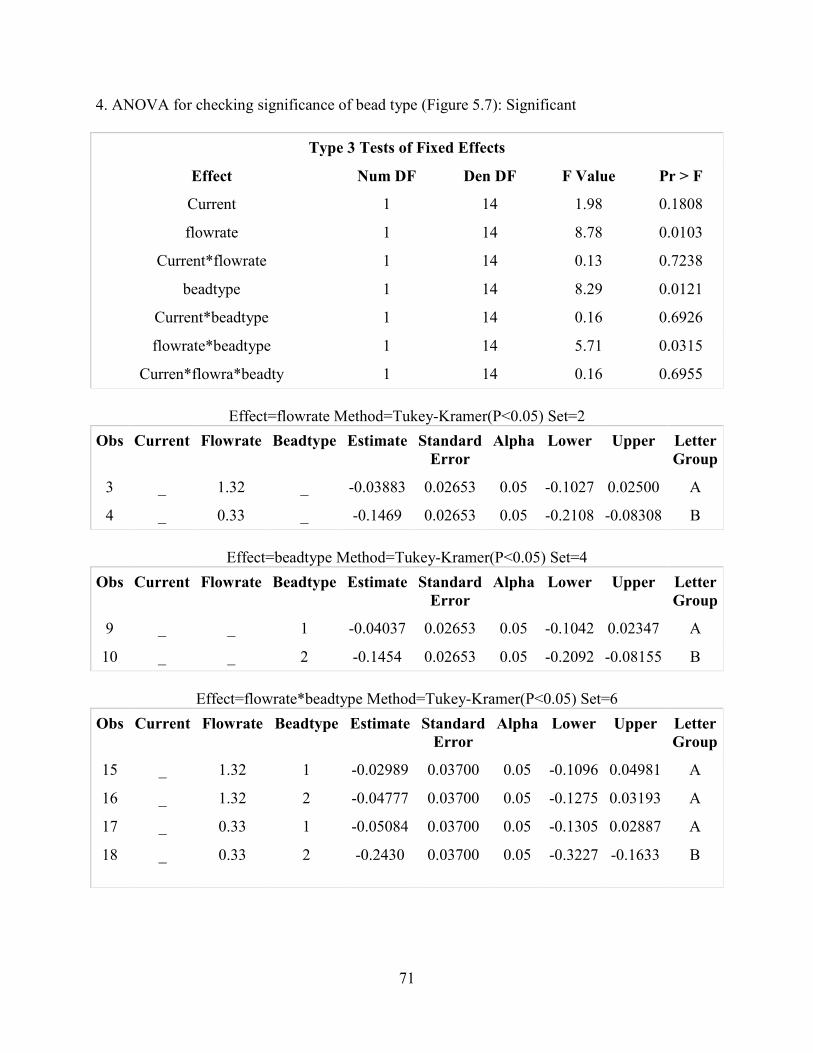
71

4. ANOVA for checking significance of bead type (Figure 5.7): Significant

Type 3 Tests of Fixed Effects

Effect Num DF Den DF F Value Pr > F

Current 1 14 1.98 0.1808

flowrate 1 14 8.78 0.0103

Current*flowrate 1 14 0.13 0.7238

beadtype 1 14 8.29 0.0121

Current*beadtype 1 14 0.16 0.6926

flowrate*beadtype 1 14 5.71 0.0315

Curren*flowra*beadty 1 14 0.16 0.6955

Effect=flowrate Method=Tukey-Kramer(P<0.05) Set=2

Obs Current Flowrate Beadtype Estimate Standard Error

Alpha Lower Upper Letter Group

3 _ 1.32 _ -0.03883 0.02653 0.05 -0.1027 0.02500 A

4 _ 0.33 _ -0.1469 0.02653 0.05 -0.2108 -0.08308 B

Effect=beadtype Method=Tukey-Kramer(P<0.05) Set=4

Obs Current Flowrate Beadtype Estimate Standard Error

Alpha Lower Upper Letter Group

9 _ _ 1 -0.04037 0.02653 0.05 -0.1042 0.02347 A

10 _ _ 2 -0.1454 0.02653 0.05 -0.2092 -0.08155 B

Effect=flowrate*beadtype Method=Tukey-Kramer(P<0.05) Set=6

Obs Current Flowrate Beadtype Estimate Standard Error

Alpha Lower Upper Letter Group

15 _ 1.32 1 -0.02989 0.03700 0.05 -0.1096 0.04981 A

16 _ 1.32 2 -0.04777 0.03700 0.05 -0.1275 0.03193 A

17 _ 0.33 1 -0.05084 0.03700 0.05 -0.1305 0.02887 A

18 _ 0.33 2 -0.2430 0.03700 0.05 -0.3227 -0.1633 B

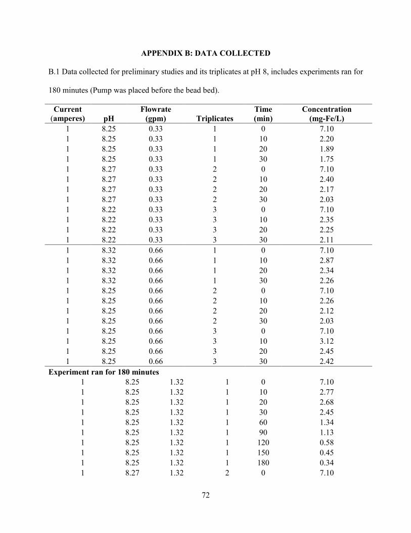
72

APPENDIX B: DATA COLLECTED

B.1 Data collected for preliminary studies and its triplicates at pH 8, includes experiments ran for

180 minutes (Pump was placed before the bead bed).

Current (amperes) pH

Flowrate (gpm) Triplicates

Time (min)

Concentration (mg-Fe/L)

1 8.25 0.33 1 0 7.10 1 8.25 0.33 1 10 2.20 1 8.25 0.33 1 20 1.89 1 8.25 0.33 1 30 1.75 1 8.27 0.33 2 0 7.10 1 8.27 0.33 2 10 2.40 1 8.27 0.33 2 20 2.17 1 8.27 0.33 2 30 2.03 1 8.22 0.33 3 0 7.10 1 8.22 0.33 3 10 2.35 1 8.22 0.33 3 20 2.25 1 8.22 0.33 3 30 2.11

1 8.32 0.66 1 0 7.10 1 8.32 0.66 1 10 2.87 1 8.32 0.66 1 20 2.34 1 8.32 0.66 1 30 2.26 1 8.25 0.66 2 0 7.10 1 8.25 0.66 2 10 2.26 1 8.25 0.66 2 20 2.12 1 8.25 0.66 2 30 2.03 1 8.25 0.66 3 0 7.10 1 8.25 0.66 3 10 3.12 1 8.25 0.66 3 20 2.45 1 8.25 0.66 3 30 2.42

Experiment ran for 180 minutes 1 8.25 1.32 1 0 7.10 1 8.25 1.32 1 10 2.77 1 8.25 1.32 1 20 2.68 1 8.25 1.32 1 30 2.45 1 8.25 1.32 1 60 1.34 1 8.25 1.32 1 90 1.13 1 8.25 1.32 1 120 0.58 1 8.25 1.32 1 150 0.45 1 8.25 1.32 1 180 0.34 1 8.27 1.32 2 0 7.10

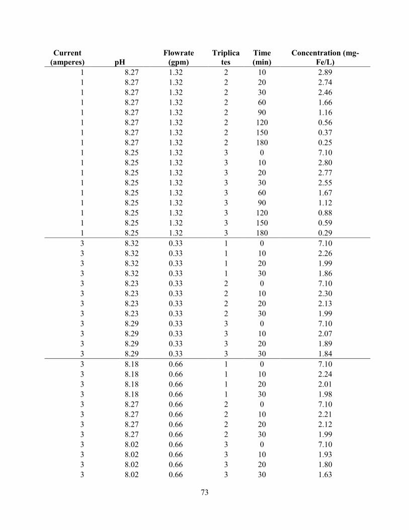
73

Current (amperes) pH

Flowrate (gpm)

Triplicates

Time (min)

Concentration (mg-Fe/L)

1 8.27 1.32 2 10 2.89 1 8.27 1.32 2 20 2.74 1 8.27 1.32 2 30 2.46 1 8.27 1.32 2 60 1.66 1 8.27 1.32 2 90 1.16 1 8.27 1.32 2 120 0.56 1 8.27 1.32 2 150 0.37 1 8.27 1.32 2 180 0.25 1 8.25 1.32 3 0 7.10 1 8.25 1.32 3 10 2.80 1 8.25 1.32 3 20 2.77 1 8.25 1.32 3 30 2.55 1 8.25 1.32 3 60 1.67 1 8.25 1.32 3 90 1.12 1 8.25 1.32 3 120 0.88 1 8.25 1.32 3 150 0.59 1 8.25 1.32 3 180 0.29

3 8.32 0.33 1 0 7.10 3 8.32 0.33 1 10 2.26 3 8.32 0.33 1 20 1.99 3 8.32 0.33 1 30 1.86 3 8.23 0.33 2 0 7.10 3 8.23 0.33 2 10 2.30 3 8.23 0.33 2 20 2.13 3 8.23 0.33 2 30 1.99 3 8.29 0.33 3 0 7.10 3 8.29 0.33 3 10 2.07 3 8.29 0.33 3 20 1.89 3 8.29 0.33 3 30 1.84

3 8.18 0.66 1 0 7.10 3 8.18 0.66 1 10 2.24 3 8.18 0.66 1 20 2.01 3 8.18 0.66 1 30 1.98 3 8.27 0.66 2 0 7.10 3 8.27 0.66 2 10 2.21 3 8.27 0.66 2 20 2.12 3 8.27 0.66 2 30 1.99 3 8.02 0.66 3 0 7.10 3 8.02 0.66 3 10 1.93 3 8.02 0.66 3 20 1.80 3 8.02 0.66 3 30 1.63

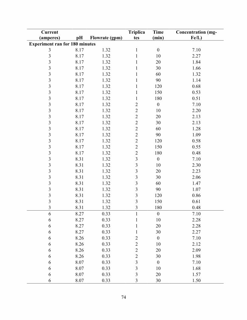
74

Current (amperes) pH Flowrate (gpm)

Triplicates

Time (min)

Concentration (mg-Fe/L)

Experiment ran for 180 minutes 3 8.17 1.32 1 0 7.10 3 8.17 1.32 1 10 2.27 3 8.17 1.32 1 20 1.84 3 8.17 1.32 1 30 1.66 3 8.17 1.32 1 60 1.32 3 8.17 1.32 1 90 1.14 3 8.17 1.32 1 120 0.68 3 8.17 1.32 1 150 0.53 3 8.17 1.32 1 180 0.51 3 8.17 1.32 2 0 7.10 3 8.17 1.32 2 10 2.20 3 8.17 1.32 2 20 2.13 3 8.17 1.32 2 30 2.13 3 8.17 1.32 2 60 1.28 3 8.17 1.32 2 90 1.09 3 8.17 1.32 2 120 0.58 3 8.17 1.32 2 150 0.55 3 8.17 1.32 2 180 0.48 3 8.31 1.32 3 0 7.10 3 8.31 1.32 3 10 2.30 3 8.31 1.32 3 20 2.23 3 8.31 1.32 3 30 2.06 3 8.31 1.32 3 60 1.47 3 8.31 1.32 3 90 1.07 3 8.31 1.32 3 120 0.86 3 8.31 1.32 3 150 0.61 3 8.31 1.32 3 180 0.48

6 8.27 0.33 1 0 7.10 6 8.27 0.33 1 10 2.28 6 8.27 0.33 1 20 2.28 6 8.27 0.33 1 30 2.27 6 8.26 0.33 2 0 7.10 6 8.26 0.33 2 10 2.12 6 8.26 0.33 2 20 2.09 6 8.26 0.33 2 30 1.98 6 8.07 0.33 3 0 7.10 6 8.07 0.33 3 10 1.68 6 8.07 0.33 3 20 1.57 6 8.07 0.33 3 30 1.50

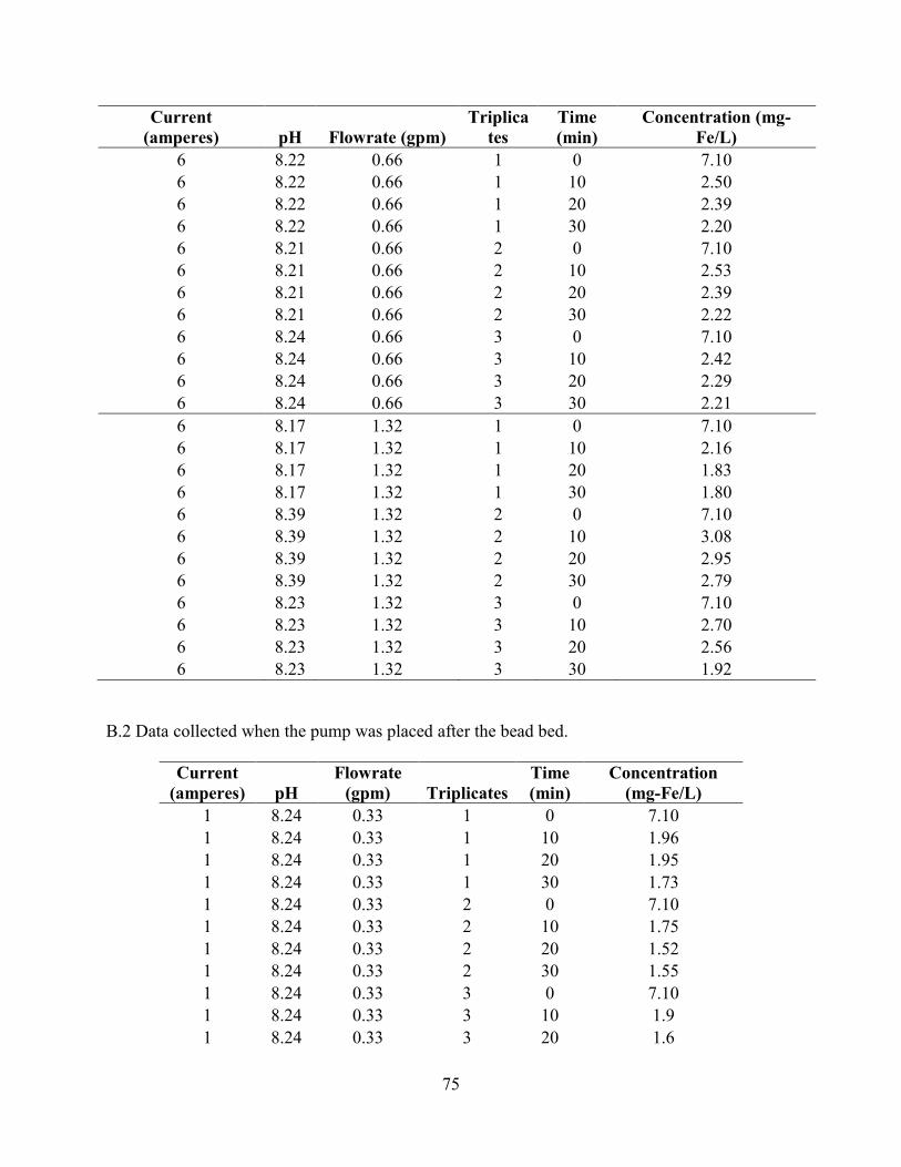
75

Current (amperes) pH Flowrate (gpm)

Triplicates

Time (min)

Concentration (mg-Fe/L)

6 8.22 0.66 1 0 7.10 6 8.22 0.66 1 10 2.50 6 8.22 0.66 1 20 2.39 6 8.22 0.66 1 30 2.20 6 8.21 0.66 2 0 7.10 6 8.21 0.66 2 10 2.53 6 8.21 0.66 2 20 2.39 6 8.21 0.66 2 30 2.22 6 8.24 0.66 3 0 7.10 6 8.24 0.66 3 10 2.42 6 8.24 0.66 3 20 2.29 6 8.24 0.66 3 30 2.21

6 8.17 1.32 1 0 7.10 6 8.17 1.32 1 10 2.16 6 8.17 1.32 1 20 1.83 6 8.17 1.32 1 30 1.80 6 8.39 1.32 2 0 7.10 6 8.39 1.32 2 10 3.08 6 8.39 1.32 2 20 2.95 6 8.39 1.32 2 30 2.79

6 8.23 1.32 3 0 7.10 6 8.23 1.32 3 10 2.70 6 8.23 1.32 3 20 2.56 6 8.23 1.32 3 30 1.92

B.2 Data collected when the pump was placed after the bead bed.

Current (amperes) pH

Flowrate (gpm) Triplicates

Time (min)

Concentration (mg-Fe/L)

1 8.24 0.33 1 0 7.10

1 8.24 0.33 1 10 1.96 1 8.24 0.33 1 20 1.95

1 8.24 0.33 1 30 1.73 1 8.24 0.33 2 0 7.10 1 8.24 0.33 2 10 1.75

1 8.24 0.33 2 20 1.52 1 8.24 0.33 2 30 1.55

1 8.24 0.33 3 0 7.10 1 8.24 0.33 3 10 1.9

1 8.24 0.33 3 20 1.6

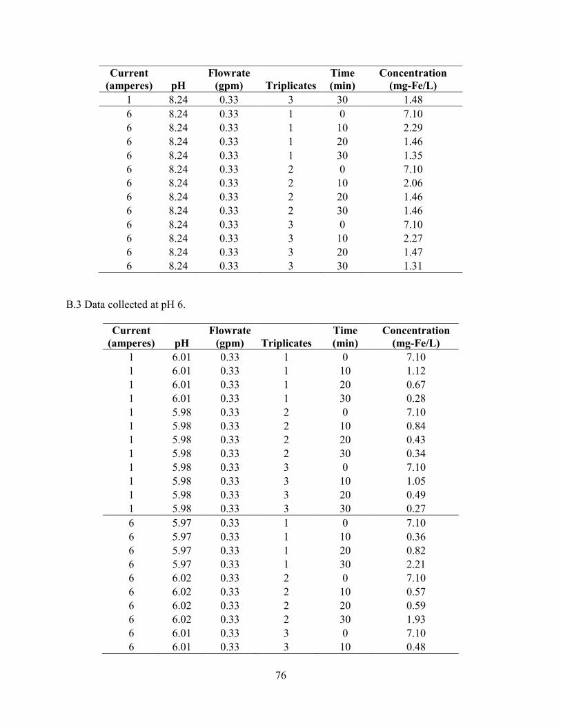
76

Current (amperes) pH

Flowrate (gpm) Triplicates

Time (min)

Concentration (mg-Fe/L)

1 8.24 0.33 3 30 1.48

6 8.24 0.33 1 0 7.10

6 8.24 0.33 1 10 2.29 6 8.24 0.33 1 20 1.46

6 8.24 0.33 1 30 1.35 6 8.24 0.33 2 0 7.10 6 8.24 0.33 2 10 2.06

6 8.24 0.33 2 20 1.46 6 8.24 0.33 2 30 1.46

6 8.24 0.33 3 0 7.10 6 8.24 0.33 3 10 2.27 6 8.24 0.33 3 20 1.47

6 8.24 0.33 3 30 1.31

B.3 Data collected at pH 6.

Current (amperes) pH

Flowrate (gpm) Triplicates

Time (min)

Concentration (mg-Fe/L)

1 6.01 0.33 1 0 7.10 1 6.01 0.33 1 10 1.12 1 6.01 0.33 1 20 0.67 1 6.01 0.33 1 30 0.28 1 5.98 0.33 2 0 7.10 1 5.98 0.33 2 10 0.84 1 5.98 0.33 2 20 0.43 1 5.98 0.33 2 30 0.34 1 5.98 0.33 3 0 7.10 1 5.98 0.33 3 10 1.05 1 5.98 0.33 3 20 0.49 1 5.98 0.33 3 30 0.27

6 5.97 0.33 1 0 7.10 6 5.97 0.33 1 10 0.36 6 5.97 0.33 1 20 0.82 6 5.97 0.33 1 30 2.21 6 6.02 0.33 2 0 7.10 6 6.02 0.33 2 10 0.57 6 6.02 0.33 2 20 0.59 6 6.02 0.33 2 30 1.93 6 6.01 0.33 3 0 7.10 6 6.01 0.33 3 10 0.48

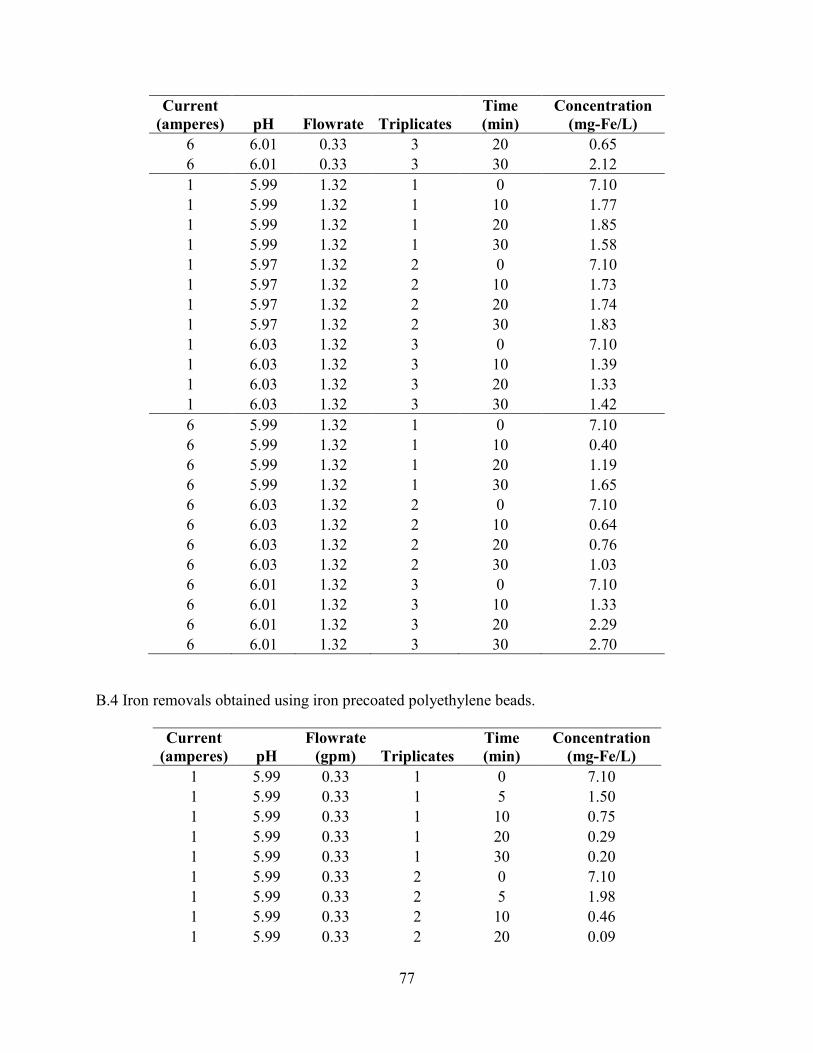
77

Current (amperes) pH Flowrate Triplicates

Time (min)

Concentration (mg-Fe/L)

6 6.01 0.33 3 20 0.65 6 6.01 0.33 3 30 2.12

1 5.99 1.32 1 0 7.10 1 5.99 1.32 1 10 1.77 1 5.99 1.32 1 20 1.85 1 5.99 1.32 1 30 1.58 1 5.97 1.32 2 0 7.10 1 5.97 1.32 2 10 1.73 1 5.97 1.32 2 20 1.74 1 5.97 1.32 2 30 1.83 1 6.03 1.32 3 0 7.10 1 6.03 1.32 3 10 1.39 1 6.03 1.32 3 20 1.33 1 6.03 1.32 3 30 1.42

6 5.99 1.32 1 0 7.10 6 5.99 1.32 1 10 0.40 6 5.99 1.32 1 20 1.19 6 5.99 1.32 1 30 1.65 6 6.03 1.32 2 0 7.10 6 6.03 1.32 2 10 0.64 6 6.03 1.32 2 20 0.76 6 6.03 1.32 2 30 1.03 6 6.01 1.32 3 0 7.10 6 6.01 1.32 3 10 1.33 6 6.01 1.32 3 20 2.29 6 6.01 1.32 3 30 2.70

B.4 Iron removals obtained using iron precoated polyethylene beads.

Current (amperes) pH

Flowrate (gpm) Triplicates

Time (min)

Concentration (mg-Fe/L)

1 5.99 0.33 1 0 7.10 1 5.99 0.33 1 5 1.50 1 5.99 0.33 1 10 0.75

1 5.99 0.33 1 20 0.29 1 5.99 0.33 1 30 0.20

1 5.99 0.33 2 0 7.10 1 5.99 0.33 2 5 1.98 1 5.99 0.33 2 10 0.46

1 5.99 0.33 2 20 0.09

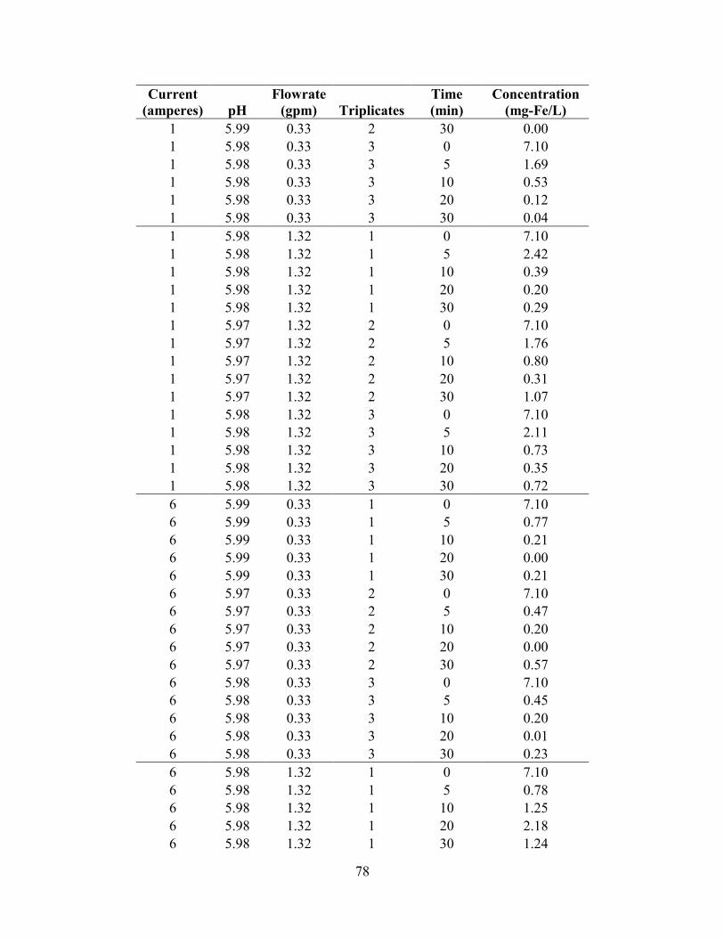
78

Current (amperes) pH

Flowrate (gpm) Triplicates

Time (min)

Concentration (mg-Fe/L)

1 5.99 0.33 2 30 0.00 1 5.98 0.33 3 0 7.10

1 5.98 0.33 3 5 1.69 1 5.98 0.33 3 10 0.53 1 5.98 0.33 3 20 0.12

1 5.98 0.33 3 30 0.04

1 5.98 1.32 1 0 7.10

1 5.98 1.32 1 5 2.42 1 5.98 1.32 1 10 0.39

1 5.98 1.32 1 20 0.20 1 5.98 1.32 1 30 0.29 1 5.97 1.32 2 0 7.10

1 5.97 1.32 2 5 1.76 1 5.97 1.32 2 10 0.80

1 5.97 1.32 2 20 0.31 1 5.97 1.32 2 30 1.07

1 5.98 1.32 3 0 7.10 1 5.98 1.32 3 5 2.11 1 5.98 1.32 3 10 0.73

1 5.98 1.32 3 20 0.35 1 5.98 1.32 3 30 0.72

6 5.99 0.33 1 0 7.10 6 5.99 0.33 1 5 0.77

6 5.99 0.33 1 10 0.21 6 5.99 0.33 1 20 0.00

6 5.99 0.33 1 30 0.21 6 5.97 0.33 2 0 7.10 6 5.97 0.33 2 5 0.47

6 5.97 0.33 2 10 0.20 6 5.97 0.33 2 20 0.00

6 5.97 0.33 2 30 0.57 6 5.98 0.33 3 0 7.10 6 5.98 0.33 3 5 0.45

6 5.98 0.33 3 10 0.20 6 5.98 0.33 3 20 0.01

6 5.98 0.33 3 30 0.23

6 5.98 1.32 1 0 7.10

6 5.98 1.32 1 5 0.78 6 5.98 1.32 1 10 1.25

6 5.98 1.32 1 20 2.18 6 5.98 1.32 1 30 1.24

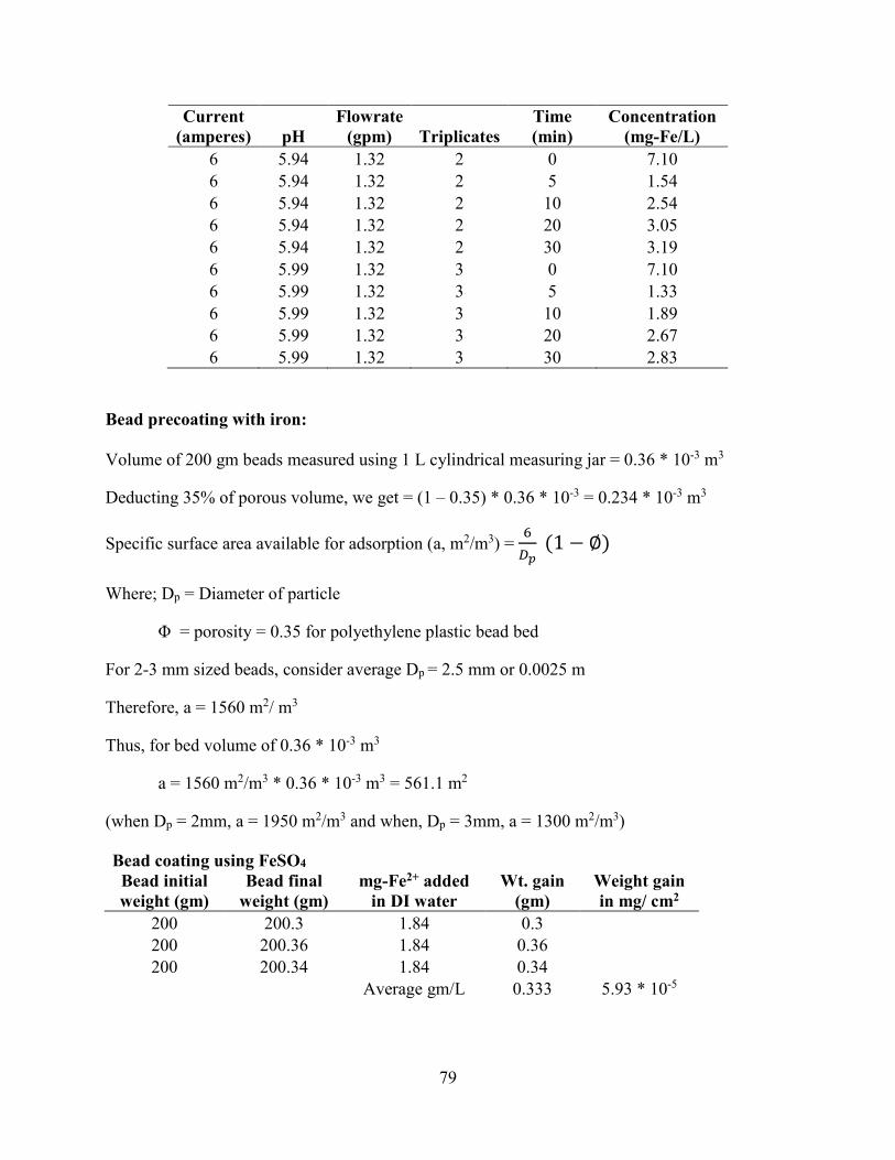
79

Current (amperes) pH

Flowrate (gpm) Triplicates

Time (min)

Concentration (mg-Fe/L)

6 5.94 1.32 2 0 7.10 6 5.94 1.32 2 5 1.54

6 5.94 1.32 2 10 2.54 6 5.94 1.32 2 20 3.05 6 5.94 1.32 2 30 3.19

6 5.99 1.32 3 0 7.10 6 5.99 1.32 3 5 1.33

6 5.99 1.32 3 10 1.89 6 5.99 1.32 3 20 2.67 6 5.99 1.32 3 30 2.83

Bead precoating with iron:

Volume of 200 gm beads measured using 1 L cylindrical measuring jar = 0.36 * 10-3 m3

Deducting 35% of porous volume, we get = (1 – 0.35) * 0.36 * 10-3 = 0.234 * 10-3 m3

Specific surface area available for adsorption (a, m2/m3) = �

��(1 − ∅)

Where; Dp = Diameter of particle

Φ = porosity = 0.35 for polyethylene plastic bead bed

For 2-3 mm sized beads, consider average Dp = 2.5 mm or 0.0025 m

Therefore, a = 1560 m2/ m3

Thus, for bed volume of 0.36 * 10-3 m3

a = 1560 m2/m3 * 0.36 * 10-3 m3 = 561.1 m2

(when Dp = 2mm, a = 1950 m2/m3 and when, Dp = 3mm, a = 1300 m2/m3)

Bead coating using FeSO4 Bead initial weight (gm)

Bead final weight (gm)

mg-Fe2+ added in DI water

Wt. gain (gm)

Weight gain in mg/ cm2

200 200.3 1.84 0.3 200 200.36 1.84 0.36 200 200.34 1.84 0.34

Average gm/L 0.333 5.93 * 10-5

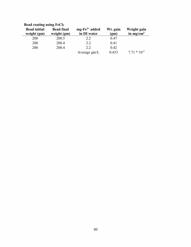
80

Bead coating using FeCl2

Bead initial weight (gm)

Bead final weight (gm)

mg-Fe2+ added in DI water

Wt. gain (gm)

Weight gain in mg/cm2

200 200.5 2.2 0.47 200 200.4 2.2 0.41 200 200.4 2.2 0.42

Average gm/L 0.433 7.71 * 10-5

81

VITA

Asmita, was born in Pune, India in 1988. She received her Bachelor’s in Civil

Engineering from Government Engineering College, Aurangabad, Maharashtra, India in 2010.

After gaining a year's experience as an engineer in a construction firm in India, she joined LSU

in Fall 2011 to pursue her Master’s degree. Currently, she is a candidate for the degree of Master

of Science in Civil Engineering.