Embed Size (px)
Citation preview

75Is ACFTA Proper Strategy of Sustainable Poverty Alleviation?: Proof From The Depletion of Saving Rate
The outcome of Regional Free Trade Area (R-FTA) still remains a conundrum. Regional free trade
area (R-FTA) is one of the manifestations of the economy integration phenomenon. R-FTA brings many
pros and cons to the economists. It allows better allocation of resources especially by eliminating tariffs,
thus making people have higher purchasing power for goods. While the increase of purchasing power is
good for growth engine and poverty alleviation progress, this paper proves that there is potency for the
agreement to be detrimental in the long run.
The main focus in this paper is the potential impact of ACFTA to the saving rate as the shock buffer
for the poor in time of recessions and crises, where purchasing power decreases significantly. We view
the ACFTA impact through the series of net import, defined as the difference between imports from
export. We use Dynamic Panel Data (DPD) to estimate the impact of net import to the saving rate, assuming
that there is a dynamic relationship between saving rate and its lagged value. The estimation result proves
that there is a negative relationship between import and the saving per capita, which indicates the
consumptive behavior of ASEAN people under high import. Moreover, the dynamic relationship shows
that saving per capita is not persistent, meaning that the saving rate will be decreased gradually.
Therefore, we can expect that in the long rung, the savings will be depleted into nothing if we
keep letting the import flooded domestic market without imposing any pre-emptive and reactive policies.
This paper provides a set of historical estimation of the potential impact of ACFTA on saving rate and its
policy implication to endure the impact.
Keywords: : : : : Free Trade, Poverty Alleviation, Saving BehaviorFree Trade, Poverty Alleviation, Saving BehaviorFree Trade, Poverty Alleviation, Saving BehaviorFree Trade, Poverty Alleviation, Saving BehaviorFree Trade, Poverty Alleviation, Saving Behavior
JEL Classification Code: : : : : E38, F15E38, F15E38, F15E38, F15E38, F15
1 Bagus Arya Wirapati is bachelor graduate from Faculty of Economics University of Indonesia and currently serving as Pengajar Mudain Gerakan Indonesia Mengajar. [email protected]
2 Niken A.S. Kusumawardhani is bachelor graduate from Faculty of Economics University of Indonesia and currently a Master Studentat Institut D»Etudes Politiques (Sciences Po) Paris. [email protected]
IS ACFTA A PROPER STRATEGYOF SUSTAINABLE POVERTY ALLEVIATION?:
PROOF FROM THE DEPLETION OF SAVING RATE
Bagus Arya Wirapati 1 danNiken Astria Sakina Kusumawardhani 2 *****
Abstract

76 Bulletin of Monetary, Economics and Banking, July 2010
I. INTRODUCTION
According to Mid-Term National Development Plan (Rencana Pembangunan Jangka
Menengah/RPJM) 2010-2014, the government of Indonesia has targeted economic growth
rates of 5.5% in 2010, 7% in 2012, and above 7% in 2014. Meanwhile, in the National Long-
Term Development Plan (Rencana Pembangunan Jangka Panjang/RPJP) 2005-2025, the
government has targeted to achieve the prosperity of the nation at an equal level with other
middle-income countries and to maintain open unemployment rate and poverty rate of less
than 5%.
Government»s targets and efforts above are determined in order to face the free trade
agreement between Indonesia and other countries. Indonesia has many multilateral or bilateral
free trade agreements with other countries, including South Korea (2007), Japan (2007), Australia
and New Zealand (2009), India (2009), and China (2010). Those free trade agreements may
bring opportunities and threats to Indonesia economy.
The agreement of ASEAN-China Free Trade Area (ACFTA) reduced tariffs of 90 percent of
imported goods to zero. ASEAN countries, especially the developing ones (note that Singapore
is considered as developed country), will be flooded by flow of goods under ACFTA. Increase of
access to great quantity of low-price goods, in term of expenditure, would be very beneficial
for the poor. Todaro and Smith (2008, [59]) argued that an increase of the poor»s access to the
goods and services is one proof of the poverty alleviation progresses. It would increase the
fulfillment of the poor»s primary and secondary needs. Therefore, based on expenditure point
of view, the number of poverty will decrease due to the increase of the poor»s ability to access
goods under this free trade agreement.
It is indeed would reduce poverty level but the sustainability of this poverty alleviation still
remains as a conundrum. Since the poor has greater marginal propensity to consume than the
have, the poor will likely choose to consume more; consequently, reducing the proportion of
savings from their income. They tend to increase the consumption rather than savings for
future buffer against economic shocks and instability. This behavior will lead them to lower
level of resilience against the economic downturn. Therefore, imposing Regional Free Trade
Area, in this case ACFTA, to increase the availability low-price goods is hypothesized to be an
improper strategy for sustainable poverty alleviation, especially in the long run.
This paper aims to answer the main question of whether ACFTA is a proper strategy of
sustainable poverty alleviation. To answer such question, main goal of this paper is to get an
empirical result of relationship between net import and savings rate as a proxy of the country»s
poverty rate. The paper will be organized in following manner: chapter 2 describes about

77Is ACFTA Proper Strategy of Sustainable Poverty Alleviation?: Proof From The Depletion of Saving Rate
ACFTA. Chapter 3 presents literature review and conceptual framework of the model used in
this research. Chapter 4 explains about research methodology, while chapter 5 includes analysis
and discussion of empirical result. Finally, the summary and policy recommendation will be
presented in chapter 6.
II. ASEAN-CHINA FREE TRADE AGREEMENT (ACFTA)
Regional Free Trade Area (R-FTA) is one of the manifestations of the economy integration
phenomenon. R-FTA brings many pros and cons to the economists. It allows better allocation of
resources especially by eliminating tariffs, thus making people have higher purchasing power for
goods. ASEAN-China Free Trade Area (ACFTA) is implemented by eliminating or reducing barriers
to trade in goods (both tariff and non tariff), improving access to service market and also investment
rules and regulations, as well as improvement of economic cooperation in order to improve the
welfare of ASEAN and China community. ACFTA brings various fortunes for ASEAN countries, as
well as its misfortunes. Government of Indonesia hopes that ACFTA will bring future favorable
implications, such as wider opportunity for Indonesia to enter China markets by means of relatively
low tariff and large population, increased cooperation between businessmen in both countries
through the establishment of strategic alliances, increased purchasing power of China goods
due to reduced tariffs or costs, and improved possibility of transfer of technology between
business people in both countries. Whether the expectations will turn into reality or not, it still
takes many years to come to finally see the actual impact of ACFTA.
Chinese Premier Zhu Rongji originated the idea of a free trade area between China and
ASEAN at the China-ASEAN Summit, November 2000. In October 2001, a group of economic
experts from China and ASEAN issued a recommendation for establishment of ASEAN-China
within ten years in the future. A month later, in November 2001, during another China-ASEAN
Summit, the leaders from respected countries started to negotiate the possibility for such an
idea. A year later, the ASEAN leaders and Chinese Premier Zhu Rongji signed the ACFTA
Framework Agreement. This agreement served as a roadmap for the establishment of the free
trade area between China and ASEAN. The agreement stated that the free trade area should be
completed by 2010, considering that four ASEAN members are expected to join the network by
2015. The ACFTA Framework Agreement is a groundbreaking document, for while individual
ASEAN members had previously created free trade agreements, ASEAN as an organization had
never before made such a bond with an outside nation. Moreover, the ACFTA Framework
Agreement was China»s first free trade agreement with a foreign nation. Since the ACFTA
Framework Agreement, both China and ASEAN have entered into negotiations with other
countries regarding free trade agreements.

78 Bulletin of Monetary, Economics and Banking, July 2010
According to ACFTA agreement, tariff elimination should be done gradually. The steps
are Early Harvest Program (EHP), Normal Track I and II, and Sensitive/Highly Sensitive List. Each
step is scheduled between each ASEAN countries and China bilaterally, which means that each
country decides its own schedule for tariff reduction or elimination for each category of product.
Since November 2002, ASEAN 6 (Indonesia, Singapore, Thailand, Malaysia, Philippine, Brunei)
and China have agreed to sign ACFTA, for 0% entry tariff per January 2004 exclusively for
products categorized as EHP. Beginning from 2004, each year Indonesia reduced tariff for
imported products from China. During 2004-2009, around 65% Chinese products have been
identified as free-entry products from Dirjen Bea Cukai, Indonesia Ministry of Finance. In January
2010, around 1598 or 18% products form China received reduction of 5% tariff while 82% of
total 8.738 import products from China have been completely excluded from tariff charge. On
the contrary, during 2004-2009, balance of trade between Indonesia and China showed that
Indonesia imports more products from China rather than exports. Therefore, during 2003-
2009, Indonesia has accumulatively a trade deficit (on non-oil trading) with China as of USD
12.6 million (around 120 trillion Rupiah). Compared to other ASEAN countries, Singapore is
the biggest exporter to China, while Indonesia is at the 5th ranking right after Thailand. The
biggest deficit of trade between Indonesia and China is around USD 7.2 million in 2008.
Indonesia»s participation in various agreements of free trade agreements can not be
prevented or reversed, although the manufacturing sector expressed its reluctance due to fear
of competition. However, typically in the agreement of free trade, there are clauses that provide
opportunity for involved parties to modify and ability to temporary suspense the concessions in
order to improve its competitiveness or strength. To protect the manufacturing sector from the
invasion of import products, government should enacted cross-ministries coordination that
involves representatives from real sector and related associations.
Since the establishment of ACFTA this January 2010, negative reactions from the
associations of real sector players have been heard. Most of them stated that they are not ready
yet to compete with China, and they asked for the government to postpone the implementation
of ACFTA agreement. Especially for the case of ACFTA and Common Effective Preferential
Tariff-ASEAN Free Trade Agreement (CEPT-AFTA), Indonesia still agree to reduce the tariff
according to schedule, where products categorized as Normal Track (NT1) ACFTA and Inclusion
List (IL) CEPT-AFTA for ASEAN planned to have 0% of entry tariff beginning January 1, 2010.
The Minister of Trade has postponed the elimination of entry tariff for some products due to
unpreparedness of some domestic sectors. At the moment being, Indonesia is in the process of
postponing tariff cut in 227 categories of product.

79Is ACFTA Proper Strategy of Sustainable Poverty Alleviation?: Proof From The Depletion of Saving Rate
III. REVIEW LITERATURE
III.1. The Role of Saving For an Economy
Savings plays an important role for an economy and each type of savings plays different
important roles. Savings are done by three entities in an economy: households, companies, and
government. Households save to cover expenses of their children and for future buffer during
retirement period. Companies retain a part of their profit as retained earning for future investment
to expand their businesses. On the other hand, government saves if the tax revenue exceeds
the government expenditure. Government saves to build public facilities or infrastructures such
as hospitals, bridges, or harbors. Lack of savings by each entity leads to different impact.
Households may have to struggle to fund their big expenses, so they have to make big loans to
banks for school expenses. If companies save too little, for example they disburse all their
income for shareholders in form of dividends; they may find it hard to fund the expansion of
their branches. Therefore, the companies lose their potential to grow. Government who saves
too little also will not be able to build physical infrastructure, and it is going to affect the
economy of the country as a whole. Foreign investors would not prefer to invest in the country
due to lack of infrastructure, and domestically, less development by government means higher
rate of unemployment and sub-optimal economic growth.
In order to possess high level of national income or prosperity, firstly a country must
possess high level of productivity. Determinants of productivity are working capitals such as
physical capital, human capital, natural resources, and technological knowledge. The more
working capitals a country has, the faster it grows compared to the others. Possession of
working capitals determines the level of productivity that a country may achieve. It»s clear to
see that one way to improve one country»s productivity is to invest its resources in form of
working capitals. The endogenous growth theories since the mid 1980s by Romer (1986,
1990), Lucas (1988), and Barro (1990) in Mikesell and Zinser (1973, [41]) confirmed the view
that the accumulation of physical capital is the critical driver of long-run economic growth.
Investment in working capital should be translated as increased saving rate of the country
itself. It»s because more usage of resources today to produce working capitals means reducing
resources available to for consumption at the time being. Reduced consumption means
increased saving. Therefore, we can conclude that more saving allows better investment in
working capitals and productivity, which in the future will lead to higher level of national
income. Development economists regard saving rate as a key performance indicator, and it is
labeled as a primary condition for achieving a satisfactory rate of economic growth (Mikesell
and Zinser, 1973, [41]).

80 Bulletin of Monetary, Economics and Banking, July 2010
A classic view of the macro-economic dynamics of the growth process was that increasing
savings when transformed into productive investment would help achieve an economic growth
(Harrod, 1939; Domar, 1946; Lewis, 1954; Solow, 1956 in AlFoul (2010, [1])). These studies
provide empirical support for hypotheses that savings growth promotes economic growth. The
conventional perception is that savings contribute to higher investment and hence higher GDP
growth in the short run (Japelli and Pagano, 1994, [32]). Finally, a study by AlFoul (2010, [1])
confirmed that during period of 1965-2007 in Morocco, a long-run two-way relationship
between real GDP and real gross domestic saving (GDS) is proved to be exist; while in the same
period in Tunisia, the results reveal that saving stimulates growth, not the other way around.
Supported by previous studies, we believe that higher savings would lead to higher growth
rate. Saving itself is defined as the result of income deducted by consumption, or can be
expressed by S = Y √ T √ C, where S = saving, Y = income, T = tax, and C = consumption.
Figure IV.1.Consumption Function
Source: Azzopardi (2004, [4])
Consumption Consumption = Disposable Income
Negative Saving
Positive Saving
Consumption FunctionC = a + c (Y-T)
a 45 degree
Disposable Income
The consumption function in the Figure IV.1 above states that consumption equals a
fixed amount of «a» plus a fraction «c» of disposable income (Y-T). A household has positive
saving when its disposable income exceeds its consumption, and it has negative saving when
its consumption exceeds its disposable income. Priorities of consumption of each household
may differ one another, but generally the basic necessities will be on the top of consumption
list. For example, during economic crisis and income falls very low, households take out their
money from savings to buy basic necessities of their life. Keynes concluded in his book, ≈The
General Theory of Employment, Interest, and Money∆, that savings depends on disposable
income. The conventional wisdom is that rich people save larger fraction of their disposable
income compared to poor people. Poor people have less disposable income, and generally they
spend all of their income for their needs, making them have no chance to save. Therefore, we

81Is ACFTA Proper Strategy of Sustainable Poverty Alleviation?: Proof From The Depletion of Saving Rate
assume that the poor has lower marginal propensity to save compared to the rich. When poor
people begin to save or to save more than they used to, it»s a signal that their wealth is improving.
II.2 Determinants of Saving Rate
Savings has been considered a critical macro-economic variable with micro-economic
foundation for achieving price stability and promoting employment opportunities thereby
contributing to sustainable economic growth (Mishra et al., 2010, [42]). As Keynes said that
saving depends on disposable income, we should criticize whether there is a dynamic relationship
between saving rate and its lagged value. People do not get higher disposable income all of a
sudden, there»s a process that people usually go through to earn high level of income. Since
previous period»s disposable income usually relates to disposable income of the next period, the
same should apply for saving rate. Higgins and Williamson (1996, [23]) estimated the relationship
for 16 Asian countries from 1950 to 1992, using IMF data on savings rates, and Penn World
Table (PWT) data on income and prices, and demographic data from United Nations database.
Higgins and Williamson (1996, [23]) used lagged value of savings, dependency ratio, annual
growth in real GDP, and relative price of investment good which encouraged saving as explanatory
variables for savings (Schultz, 2004, [54]). This equation becomes unique because it assumes
there is a dynamic relationship between saving rate (Sti) and its lagged value (St-1). Schultz
(2004, [54]) contended that saving rate is expected to change gradually over time to new
condition, and a year is not an adequate time for saving rate to achieve its new condition.
Saving rate should adapt in more than a year period, adjusting to individual»s level of disposable
income. Since we assume that saving rate of period t has a relationship with saving rate at
period t-1, it implies that whatever errors are present in the savings equation in one year will
not be independent of the error in savings in the prior or following years (Schultz, 2004, [54]).
This dynamic relationship of saving and its lagged value shows that lagged value of saving
should be included as one of the determinants of saving rate as a dependent variable.
Government saves if its revenue from taxes exceeds its spending. The summary of
government activities of spending and receiving tax revenue can be seen in its budget balance.
According to Keynesian open-economy model, there is a positive association between budget
balance and trade balance. In Keynesian open-economy model, budget deficit may lead to
trade deficit. The higher budget deficits put upward pressures on interest rates, where higher
interest rates would raise the foreign exchange value of the currency, and the stronger currency
would in turn reduce net exports, in other words, trade deficit. However, this conventional
view of the twin deficits has not gained much empirical support. Evans (1985, 1986) in Darrat
(1988, [12]) has found no reliable relationship for the US between budget deficits on the one

82 Bulletin of Monetary, Economics and Banking, July 2010
hand and either interest rates or exchange rates on the other. The empirical evidence is somewhat
less ambiguous and suggests that trade deficits in the US are inversely related to the exchange
value of the dollar, though the response is both small and sluggish. Proponents of this
conventional view found partial relationship between higher budget deficits and higher interest
rates (Plosser (1982, [46]), Hoelscher (1983, [25]), Cebula (1987, [10]), and Wachtel and Young
(1987, [60]). The other proponents such as Feldstein (1982) in Islam (1998, [30]) concluded
that larger budget deficits result in higher interest rates, which causes the appreciation of
exchange rate, thereby worsening the trade imbalance.
Different empirical results of the relationship between the twin deficits attracted more
research in respected topic. Another hypotheses being developed were (1) trade deficits because
budget deficits, (2) the two deficits are causally independent, and (3) the two deficits have
bidirectional causality. Over the 3 hypotheses, the hypothesis of bidirectional relationship between
budget deficit and trade deficit gained much empirical support. Islam (1998, [30]) examined
the direction of causality between budget deficits and trade deficits based on Granger test for
Brazil during 1973:1Q through 1991:4Q. Based on Granger»s causality test, Islam (1998, [30])
concluded that there is a bilateral causality between trade and budget imbalances. Another
empirical result presented by Darrat (1988, [12]) also concluded that there is a mutual causality
relationship between budget and trade deficit. Darrat (1988, [12]) hypothesized that not only
budget deficit causes trade deficit, but trade deficit may also cause budget deficit. According
to Darrat (1988, [12]), when a country»s level of net export fell off (caused by other factors than
the budget deficit), the pressure on the government would be increased. Decrease in the level
of net export would harm domestic industries, leading to higher unemployment rate and loss
of foreign market shares. This situation would in turn decrease the revenue of the government
from tax, since business activities in the export sector were depressed. The government also
would spend more to stimulate the depressed sector or to give aid to harmed domestic industries.
The empirical results of Darrat (1988, [12]) only partially support the conventional view that
budget deficits caused trade deficit, but strongly support the causality between trade deficits
to budget deficits. The empirical result of Darrat (1988, [12]) and Islam (1998, [30]) supported
the view that trade deficit has bidirectional causality with budget deficit.
The Keynesian revolution based on under-employment equilibrium made saving a function
of income and income a function of investment, as opposed to the Neoclassical view of saving
as a determinant of investment (Mikesell and Zinser, 1973, [41]). Empirical tests of saving-
income relationship have been conducted in two big groups: Keynesian or non-Keynesian
hypotheses. Kuznets (1960, [25]) in Mikesell and Zinser (1973, [41]) was among the first to do
a cross-sectional study between per capita income and saving. Kuznets (1960, [25]) achieved a

83Is ACFTA Proper Strategy of Sustainable Poverty Alleviation?: Proof From The Depletion of Saving Rate
conclusion that there was a tendency for countries with high capita income to have higher
saving ratios, but the tendency was not very consistent. Singh (1971) in Mikesell and Zinser
(1973, [41]) as a proponent of the Keynesian also concluded that when per capita GNP rose
from $100 to $1000 the gross saving ratio increased by 8 percentage points. Singh (1971) also
found that at a per capita GNP growth rate of 2 percent, it would take 50 years to increase the
saving rate by 3 percentage points. On the other hand, the proponent of non-Keynesian
hypotheses came up with a very theory of saving behavior. Dusenberry (1949, [15]), Friedman
(1957, [17]), Modigliani et al. (1954, [43]) concluded a rise in per capita in- come would not
merely lead to a higher savings ratio. One of the studies, conducted by Friedman (1957, [17]),
resulted in a new hypothesis called ≈Permanent Income Hypothesis (PIH)∆. Friedman»s hypothesis
is that people consume permanent income, and all of the transitory income (difference between
actual income and permanent income) will be allocated to saving. This implies a heavy reliance
on past behavior as a determinant of consumption spending; but changes in transitory income
will immediately lead to changes in the level of saving.
Classic analyses on savings and growth have focused on two main issues: (1) the effect of
higher savings on long run growth, and (2) the impact of higher savings on investment.
Neoclassical models inspired by Solow (1956, [57]) suggested that an increase in saving ratios
generates higher growth only in the short run, during the transition between steady states
(Edwards, 1995, [16]). More recent studies by Romer (1986, [50]) predicted that higher savings
(and the related increase in capital accumulation) might lead to permanent increase in growth
rates. Proponents of this conventional perception conclude that savings contribute to higher
investment and also higher GDP growth in the short run (noted that the catching up effect and
the law of diminishing return are exist). That»s why according to Quah (1993) in Edwards (1995,
[16]) middle-income countries are slowly vanishing. As the countries are in transition to achieve
similar steady state as high-income countries, this assumption provides a basis for researchers
to study the direction of causality between growth rate and saving rate. Mohan (2006, [45])
studied about the direction of causality between growth rate and saving rate using the concept
of Granger causality. His study is supported by previous studies that revealed that higher level
of growth rate led to higher level of saving (Caroll and Weil (1994, [9]), Sinha (1996, [55]), Saltz
(1999, [52], and Anoruo and Ahmad (2001, [2]). Caroll and Weil (1994, [9]) examined the
relationship between income growth and saving using both cross-country and household data.
At the aggregate level, they found that growth causes saving, and households with higher
income growth save more than households with low growth at household level. Caroll and
Weil (1994, [9]) explained this phenomenon by using theory of habit stock effect. They contended
that initially, a country has its own saving habit. When the rate of growth is increased in the first
period of life, the country»s income is going to be increased more than its consumption, and
84 Bulletin of Monetary, Economics and Banking, July 2010
therefore increased first period saving rate. The average saving rate of a fast-growing economy
will be higher than that of a slow-growing economy (Modigliani, 1970, [44]). What makes
Mohan»s (2006, [45]) work interesting was that he divided countries that become his samples
into different income levels (LIC/LMC/UMC/HIC). The primary hypothesis of Mohan (2006, [45])
is whether the income level of the economy influences the direction of causality between
growth rate and savings. Using time series annual data, Granger causality tests were conducted.
Mohan (2006, [45]) concluded that his study favored the hypothesis that the causality is from
economic growth rate to growth rate of savings. Mohan (2006, [45]) contended that income
levels play an important role in determining the direction of causality, he argued that the
explanation of positive causality between economic growth rate and saving rate could be best
explained by the human wealth effect theory.
The relationship between interest rates and aggregate saving involves a number of complex
theoretical and econometric problems; the most important are separating out income and
substitution effects of interest changes, quantifying the role of expectations and planning
horizons in saving decisions, and solving a difficult econometric identification problem. Williamson
(1968 in Balassa (1989, [5]) in an empirical study of six Asian countries found that with the
exception of Burma, real rates of interest were negatively correlated with national savings. In
turn, Gupta (1970, [19]) found the interest elasticity of savings to be positive and statistically
significant at the 1 percent level for India, when per capita disposable income was used as
explanatory variable. A study by Yusuf and Peter (1984, [61]) concluded that a one percent rise
in the interest rate was accompanied by an approximately one percent increase in gross national
saving; i.e. an interest elasticity of savings of 1 (Balassa, 1989, [5]). Several other studies have
concentrated principally on the effects of interest rate reforms in Korea, Taiwan and Indonesia,
where increases in bank deposit rates (along with increased load rates) have been accompanied
by sharp rises in savings deposits without dampening the business demand for loans. But this
may simply entail a redirection of savings and a change in the pattern of investment toward
more productive forms rather than an increase in the saving propensity.
Inflation is a good macroeconomic proxy for stability. Several studies proved different
results concerning the relationship between inflation and saving rates. Some studies analyzed
effect of inflation and savings showed a negative effect (Heer and Suessmuth (2006, [22])).
Haan (1990) in Heer and Suessmuth (2006, [22]) found that a rise of the inflation rate from
0%-5% decreased savings by almost 10%. However, proponents of positive relationship between
saving rate and inflation are more common. Based on precautionary saving theory, households
increase their savings whenever they feel threatened by the instability of the country»s economy.
As previously said, inflation is often used as a proxy for economic stability. Consequently, savings

85Is ACFTA Proper Strategy of Sustainable Poverty Alleviation?: Proof From The Depletion of Saving Rate
will increase whenever inflation is set at a higher rate. Deaton (1977, [14]) argued that unexpected
inflation caused involuntary saving because individual consumers were not sophisticated enough
to differentiate between relative price changes and absolute price changes. This lack of possible
means for individual customers to compare relative and absolute price changes would eventually
lead them to think that all goods are relatively more expensive; so that they choose to consume
less and save more (assume real income is maintained at same level). According to Deaton
(1977, [14]), as unexpected inflation rises, saving ratio also rises. Meanwhile, Howard (1978,
[27]) argued that inflation influences saving in two different assumptions. As long as the inflation
is unexpected, it will increase saving rate, since it creates pessimism about economic stability,
so that people are encouraged to save more. But if the inflation is expected (provided in advance),
it encourages people to increase their purchase of durable goods, therefore decreasing their
savings during inflationary period.
Modern consumption theory starts with the presumption that consumers like to smooth
out consumption over time, whether over the life cycle (Modigliani and Brumberg, 1954, [43])
or in the face of temporary fluctuations to income (the permanent income hypothesis of Friedman
(1957, [17])). Life cycle saving theory from Modigliani and Brumberg (1954, [43]) suggested
that consumers tend to smooth consumption over a lifetime. Modigliani and Brumberg (1954,
[43]) assumed in their model that savings would be high when incomes are high (during
productive working age), and people will dis-save during retirement. Life-cycle theory of saving
predicts a rise in saving as the youth-dependency ratio declines in the later stages of demographic
transition. Young-dependency ratio is regarded as a constraint for saving because children
charge a heavy expenditure for the working age population. Children contribute to consumption,
but not to production. That»s why high young dependency ratio is expected to impose a constraint
for saving (Leff, 1969, [37]). Leff (1969, [37]) found that dependency ratio significantly influence
aggregate savings. High dependency ratio is also used to evaluate the disparity between
developing and developed countries. Old-dependency ratio is also regarded as another constraint
for saving in the countries with no retirement plan. The elderly will be a burden for their working
children since they have no more income, or if the retired adult still should spend some expenses
for their young children. Both cases will be constraints for saving. Formally, if adults with fewer
children have more resources available over a lifetime, and these additional resources are
consumed by the adults themselves (rather than on children»s education for example),
consumption smoothing implies that consumption will also be higher after retirement, and
hence saving for retirement will have to be higher (Attanasio et al., (1999, [3]); Scholz et al.
(2006, [53]); Skinner (2004, [56])). Many studies find evidence of an impact of the youth and
old-age dependency ratios. For the youth-dependency ratio, Rijckeghem and Üçer (2009, [48])
estimated that a 1% point reduction in this ratio is associated with a 0.3 percentage point

86 Bulletin of Monetary, Economics and Banking, July 2010
increase in the saving rate in the short-run (0.5 percentage points in the long-run). The
corresponding are 1.4 and 2.8 for the old-age dependency ratio.
IV. METHODOLOGY
IV.1. Estimation Method and Model
We use Dynamic Panel Data (DPD) model to estimate the characteristic and the
determinants of saving. We assume that there are dynamic relationship between savings and
its lagged value. We define the lagged value relationship on current savings as the persistence
of savings over time. Savings are considered as persistent if the coefficient of the lagged value
approach 1, since it means that under the rest remains constant, savings tends to be constant
over time. However, if the coefficient is significantly different from 1, savings are considered as
not persistent, since the value will change over time, either increasing or decreasing, with the
rest remain constant. Savings is increasing if the coefficient is higher than 1, and reversely
decreasing when the coefficient is lower than 1. For this estimation, we use gross domestic
savings per capita to show individual savings, replacing household savings which cannot be
used due to unavailability of data for all ASEAN countries.
The main focus on this model is the import from ASEAN countries and China as the main
variable. We use ratio of net import from ASEAN countries and China from the total GDP for
estimation. Why net import while others use net export? The reason is to simplify the
interpretation so that we put import on our main focus in trade, nor the reverse. This variable
can be explained as the contribution of the ACFTA on the total GDP of ASEAN countries. The
main hypothesis is that import from ASEAN countries and China has negative impact on the
savings, which proves that an increase in the respective import will decrease the savings, due to
an increase in consumption. We are also going to compare the elasticity of import to the
persistency of savings to see whether under the ACFTA savings will be depleted over time,
indicating an increase of the poor»s vulnerability.
In order to acquire a more accurate, precise coefficient to compare, we insert more regressor
as control variables. Their role is simply as the explanatory terms which specify the model to get
more accurate coefficients, and also for a direction in applying it to the policy implications. The
control variables in the model are as follows:
1. The income of people, represented by the GDP per capita. An increase in people»s income
provides people with more funds to save. Therefore, the relationship is expected to be positive.
2. The economic growth, defined as the percent change of current GDP from the previous
year. An increase in economic growth, which expands the economy, increase the potency of
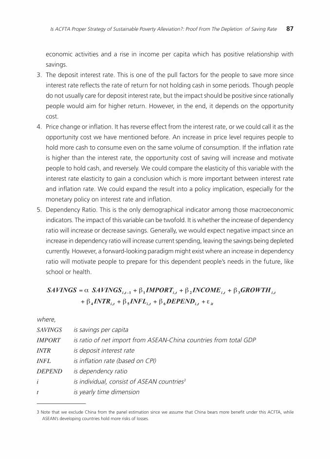
87Is ACFTA Proper Strategy of Sustainable Poverty Alleviation?: Proof From The Depletion of Saving Rate
economic activities and a rise in income per capita which has positive relationship with
savings.
3. The deposit interest rate. This is one of the pull factors for the people to save more since
interest rate reflects the rate of return for not holding cash in some periods. Though people
do not usually care for deposit interest rate, but the impact should be positive since rationally
people would aim for higher return. However, in the end, it depends on the opportunity
cost.
4. Price change or inflation. It has reverse effect from the interest rate, or we could call it as the
opportunity cost we have mentioned before. An increase in price level requires people to
hold more cash to consume even on the same volume of consumption. If the inflation rate
is higher than the interest rate, the opportunity cost of saving will increase and motivate
people to hold cash, and reversely. We could compare the elasticity of this variable with the
interest rate elasticity to gain a conclusion which is more important between interest rate
and inflation rate. We could expand the result into a policy implication, especially for the
monetary policy on interest rate and inflation.
5. Dependency Ratio. This is the only demographical indicator among those macroeconomic
indicators. The impact of this variable can be twofold. It is whether the increase of dependency
ratio will increase or decrease savings. Generally, we would expect negative impact since an
increase in dependency ratio will increase current spending, leaving the savings being depleted
currently. However, a forward-looking paradigm might exist where an increase in dependency
ratio will motivate people to prepare for this dependent people»s needs in the future, like
school or health.
ittititi
titititi
DEPENDINFLINTR
GROWTHINCOMEIMPORTSAVINGSSAVINGS
εβββ
βββα
++++
+++= −
,6,5,4
,3,2,11,
where,
SAVINGS is savings per capita
IMPORT is ratio of net import from ASEAN-China countries from total GDP
INTR is deposit interest rate
INFL is inflation rate (based on CPI)
DEPEND is dependency ratio
i is individual, consist of ASEAN countries3
t is yearly time dimension
3 Note that we exclude China from the panel estimation since we assume that China bears more benefit under this ACFTA, whileASEAN»s developing countries hold more risks of losses.

88 Bulletin of Monetary, Economics and Banking, July 2010
IV.2. Data
We estimate it using panel data of all ASEAN countries from 2000 to 2008. Since ACFTA
has not been imposed for long, we use historical data to predict the impact of ACFTA in the
present and the future. We receive data for savings per capita and import from United Nations»
UNSTATS and UNCOMTRADE. For interest rate and inflation, we use data from IMF»s International
Financial Statistics (IFS) and for dependency ratio we use data from CEIC.
The DPD methodology that we use for this model is Arellano-Bond 1st Difference GMM
due to the following reasons:
1. Relationship is existed within savings and its lagged value.
2. We assume that there are dynamic relationship within savings and economic growth, as
explained in Mohan (2006, [45]), also with the interest rate and inflation.
3. The unobserved country-specific error term (wi) in terms of demographical indicators are
correlated with the dependency ratio.
4. The country numbers as cross section data (N = 10) is relatively higher than the number of
time series. (T = 7).4
Now that we have several problems arises above, we are obliged to eliminate the problems,
which are solvable using the Arellano-Bond GMM. The Arellano-Bond GMM itself is an estimation
methodology to observe the effect of dynamic relationship between the dependent variables
and its lagged value. As for the endogeneity problem, we impose instrumental variables on the
GMM. For instrumental variables imposed in this model, we put the lagged value of the
endogenous regressor (growth, interest rate and inflation)
The third problem, correlation of unobserved country-specific error term is eliminated
using the first difference in Arellano-Bond GMM following this formula:
4 Since Arellano Bond GMM use first difference and we put first lag of savings on the model, the estimator is automatically drop twofirst observation, therefore the remaining time observation is 7.
where,
then,
wi is the unobserved country-specific error term. As we can see from the equation above, we
have eliminated the unobserved country-specific error term using the first difference term.
∆yi,t
= α1∆y
i,t-1 + α
2∆X
i,t + ∆
i,t
yi,t − y
i,t-1 = α
1 (y
i,t-1 − y
i,t-2)
+ α
2 (X
i,t − X
i,t-1) + (
i,t −
i,t-1)
i,t = w
i + u
i,t
i,t −
i,t-1 = (w
i − w
i,t)
+ (u
i,t − u
i,t-1) = u
i,t − u
i,t-1 = ∆u
i,t

89Is ACFTA Proper Strategy of Sustainable Poverty Alleviation?: Proof From The Depletion of Saving Rate
Therefore, the error term remains is vi,t which is panel data error term from the estimation.
Hence, we should worry anymore about this correlation between errors and the independent
variables since the problematic unobserved country-specific error term has been eliminated
from the estimation.
V. RESULT AND ANALYSIS
Using Arellano-Bond GMM in two-step estimation from Stata 11, we acquire the following
result:
Coef. (Std. Error) [Prob.]
Saving (-1)Saving (-1)Saving (-1)Saving (-1)Saving (-1) 0.1439227* 0.149482** 0.5340291***(0.0605343) (0.0697293) (0.0995964)
[0.022] [0.032] [0.000]ImportImportImportImportImport -5.13867 -6.781835*** -3.844283
(5.173365) (1.697932) (5.063839)[0.326] [0.000] [0.448]
IncomeIncomeIncomeIncomeIncome 0.6441702*** 0.6125879*** 0.2395092***(0.0509349) (.0662613) (0.0486907)
[0.000] [0.000] [0.000]GrowthGrowthGrowthGrowthGrowth 1.540742 10.84045 12.7541**
(3.339246) (19.5483) (6.328766)[0.647] [0.579] [0.044]
IntrIntrIntrIntrIntr 2.08293 40.2688 14.3462(10.82252) (41.9624) (12.91631)
[0.848] [0.337] [0.267]InflInflInflInflInfl -1.352008 -6.455056 3.970357
(2.637306) (8.411291) (4.28696)[0.611] [0.443] [0.354]
DependDependDependDependDepend 4.962723 12.66345* 4.704166(5.290578) (7.258577) (3.515673)
[0.354] [0.081] [0.181]
FE GMM OLSVARIABLES
*** (**) [*] significant under 1% (5%) [10%] critical value
ContinuumContinuumContinuumContinuumContinuumFE 0.1439227 UNBIASEDUNBIASEDUNBIASEDUNBIASEDUNBIASED
GMM 0.149482OLS 0.5340291
ValidityValidityValidityValidityValiditySargan 1.000000 VALIDVALIDVALIDVALIDVALID
ConsistencyConsistencyConsistencyConsistencyConsistencyM1 0.4301 INCONSISTENTINCONSISTENTINCONSISTENTINCONSISTENTINCONSISTENTM2 0.4489
GMM POST-ESTIMATION ΩΩΩΩΩ
90 Bulletin of Monetary, Economics and Banking, July 2010
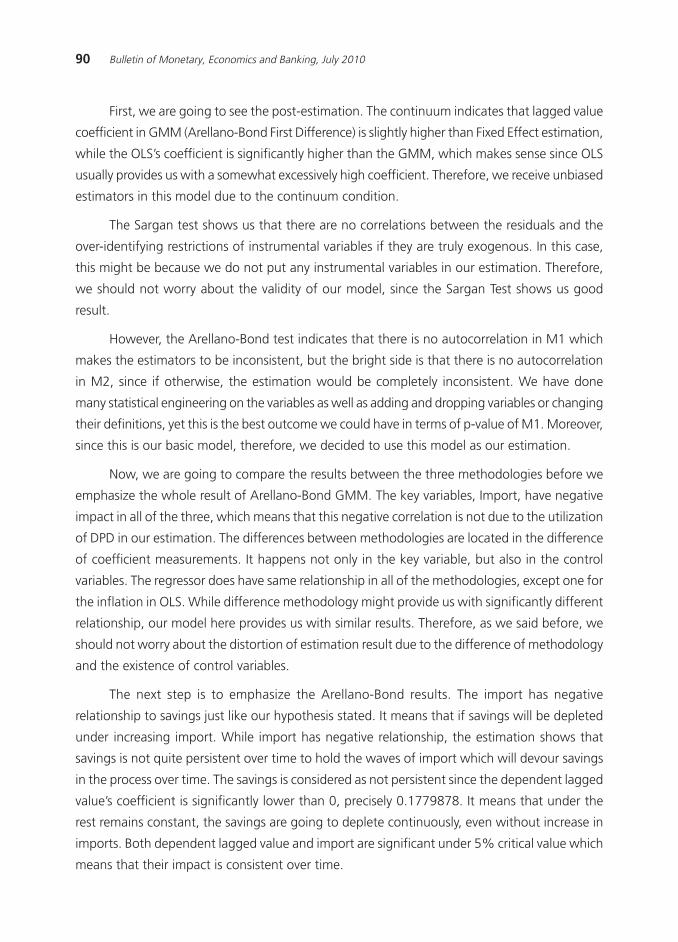
First, we are going to see the post-estimation. The continuum indicates that lagged value
coefficient in GMM (Arellano-Bond First Difference) is slightly higher than Fixed Effect estimation,
while the OLS»s coefficient is significantly higher than the GMM, which makes sense since OLS
usually provides us with a somewhat excessively high coefficient. Therefore, we receive unbiased
estimators in this model due to the continuum condition.
The Sargan test shows us that there are no correlations between the residuals and the
over-identifying restrictions of instrumental variables if they are truly exogenous. In this case,
this might be because we do not put any instrumental variables in our estimation. Therefore,
we should not worry about the validity of our model, since the Sargan Test shows us good
result.
However, the Arellano-Bond test indicates that there is no autocorrelation in M1 which
makes the estimators to be inconsistent, but the bright side is that there is no autocorrelation
in M2, since if otherwise, the estimation would be completely inconsistent. We have done
many statistical engineering on the variables as well as adding and dropping variables or changing
their definitions, yet this is the best outcome we could have in terms of p-value of M1. Moreover,
since this is our basic model, therefore, we decided to use this model as our estimation.
Now, we are going to compare the results between the three methodologies before we
emphasize the whole result of Arellano-Bond GMM. The key variables, Import, have negative
impact in all of the three, which means that this negative correlation is not due to the utilization
of DPD in our estimation. The differences between methodologies are located in the difference
of coefficient measurements. It happens not only in the key variable, but also in the control
variables. The regressor does have same relationship in all of the methodologies, except one for
the inflation in OLS. While difference methodology might provide us with significantly different
relationship, our model here provides us with similar results. Therefore, as we said before, we
should not worry about the distortion of estimation result due to the difference of methodology
and the existence of control variables.
The next step is to emphasize the Arellano-Bond results. The import has negative
relationship to savings just like our hypothesis stated. It means that if savings will be depleted
under increasing import. While import has negative relationship, the estimation shows that
savings is not quite persistent over time to hold the waves of import which will devour savings
in the process over time. The savings is considered as not persistent since the dependent lagged
value»s coefficient is significantly lower than 0, precisely 0.1779878. It means that under the
rest remains constant, the savings are going to deplete continuously, even without increase in
imports. Both dependent lagged value and import are significant under 5% critical value which
means that their impact is consistent over time.

91Is ACFTA Proper Strategy of Sustainable Poverty Alleviation?: Proof From The Depletion of Saving Rate
Now for the control variables, only income per capita and dependency ratio which is
significant under 5% critical value, while the remaining is not significant. Income per capita has
positive relationship with savings which means that an increase in income per capita will increase
the savings. Economic growth also encourages people to save since it has positive relationship
with savings. So does the interest rate. An increase in deposit interest rate brings positive
impact on the motivation of people to save. While lastly, as expected, inflation holds negative
impact on the savings since people have to hold more money.
The estimation has provided us with the required information on how import affects the
saving rate along with other macroeconomic and demographic explanatory terms. We are
going to focus more on how the regressors affect the dependent variable. Significance does
matter but even for the insignificant variables, we are still analyzing the impact of the regressor
since we can still consider the coefficient as the tendency of how the variables affect the
dependent variable.
V.1. The Savings Behavior in ASEAN
We consider the estimation result as a behavior model of savings in our specific region,
ASEAN, under flowing trade of goods within ASEAN and China. Let us recall the estimation
result of Arellano-Bond GMM for analyzing purpose.
The lagged dependent variable»s coefficient shows us the persistency of savings per capita
over time, ceteris paribus. It indicates the behavior of people to keep their savings over time in
condition where the rest remain constant. The coefficient value of lagged dependent variable is
significantly below 1.00, precisely 0.15, which means the saving per capita would decrease by
85% over time. It indicates that people will draw their savings in high proportion in order to
fulfill both their needs and wants. If we take wants into account, since needs are basic goods
that cannot be eliminated from routine consumption buckets, we could expect people tend to
become consumptive since they consume goods outside basic needs which along with the
basic needs consumption, it depletes the saving per capita by 85%. Recall that we assume the
rest remain constant, so that it means there is no adjustments of consumption under price
changes; therefore the coefficient shows only the depletion series of saving rate. Based on this
estimation, we take a simple and quick conclusion that ASEAN people weigh more on
consumptive behavior, which is a behavior that can be found in developing countries, recall
that most of ASEAN countries are developing countries.
The net import has negative impact on saving rate. It means that an increase in the
import over the export level will deplete the consumption. This is just like our hypothesis

92 Bulletin of Monetary, Economics and Banking, July 2010
stated earlier in this paper. An increase in import level, while export remains constant, will
reduce people»s savings. This is due to the increase of consumption under the increase of
goods availability in economy. As estimated before in the coefficient of saving»s lagged value,
ASEAN people tend to consume more over time in such a high proportion of 85%. This data
is estimated before the ACFTA being implemented in ASEAN (ACFTA was started in January,
2010). Therefore, we can expect that under ACFTA, the flow of goods will surely become
high as the import on ASEAN countries increases; the consumption pattern of ASEAN people
would increase. If the other variables assumed to be constant, the savings would be decreased
to nothing in a short time. But, this is not without solution. The answer for it lies on the half-
side of net import, which is the export side. The export here acts as the counter-effect of the
import that reversely will increase saving rate. This logic comes from the formula of Net
Import, which is the subtraction of import with the export. An increase in export would
decrease the net import. Therefore, the export has reverse effect from the import. An increase
in export would let people to produce more products, allowing them to gain more income
from the economic activity. For another simple explanation, the export is an additional
component of GDP, so an increase in export would increase GDP and bear the potential of
increasing income per capita.
Speaking of income per capita, the estimation shows us that the income per capita has
positive effect on the savings, and moreover has positive impact. The coefficient of this variable
is 0.61. The implication of this coefficient is that ASEAN people would provide 61% of their
income change for saving and use up to 39% of it to consume. It could also work on the
reverse, when the income per capita reduced, people will draw their savings by 69% of their
income change, since they need more liquidity to consume needs under decreasing income,
probably under recession or crisis. This is also one of the answers to endure the impact of
ACFTA that is in line with export solution. Income is surely an important component to improve
if we are aim to increase or keep savings from the community. As discussed before, export is
one of the components of GDP and income, which means that export, needs to be one our
vital solution to increase people»s income.
We might think that there is some inconsistency inside this estimation analysis. At first,
we thought that people tend to become consumptive since the persistency of savings is very
low. But, reversely, the income per capita»s coefficient shows that people distribute more of
their income change to the savings, rather than to consumption. One point that we need to
see is that the consumptive behavior we analyze first is under the assumption where the income
is constant. With constant income over time, people tends to deplete their savings to consume
more and this might be because of the insufficiency of income for ASEAN people, especially

93Is ACFTA Proper Strategy of Sustainable Poverty Alleviation?: Proof From The Depletion of Saving Rate
those who live in developing countries, to fulfill their needs and wants. Therefore, people keep
on drawing their savings to fulfill their needs and wants.
For the income change that is allocated more to the savings, the explanation might lie
within the estimation of dependency ratio parameter. The dependency ratio has significant
positive impact on saving rate. It can be explained through precautionary saving behavior theory,
but this time we relate the instability discussed in the theory to high expense that the productive
groups bear. More people depend on the productive age; more funds will be needed to prepare
for future consumption. One simplest example is for children who are still enrolling on school
or university. The parents who are in productive population must allocate more of their income
for their children educational plan. This is also shows that most of ASEAN people are a risk-
averse kind of people when they have more people under their care. However, this is not to be
proud of, since this variable only explains why people allocate more of their income change for
saving. We cannot use this variable as our hope to increase savings. Increasing dependency
ratio is surely not an answer to keep the savings rate; it is just an explanatory term.
The remaining variables are not significant; however we are still going to analyze the
insignificant impact to see the potential impact these variables can do for the saving rate.
Growth has positive impact which means that the expansion of the economy could provide
people with opportunity to increase income and furthermore the saving. This is due to rapid
growth of population that usually happens in ASEAN as a region of developing countries. An
increase in growth itself might not affect the saving rate since it might not increase the individual
income of the people. If the economic growth is not as fast as the population growth, then
basically the income per capita, our significant variable, will be decreased. That is why growth
is not significant in affecting the saving rate.
Deposit interest rate will increase saving rate since it is a proxy of return if depositors save
their funding on banks. An increase in return would encourage people to save more, in hope to
gain more return from the interest. Interest rate is not significant because return on saving is
not quite encouraging for most people. This is because most people which have only regular
income would not save huge amount of money, like about billions Rupiah. This interest rate
would not provide them with significant return if not invested in more than hundred billions
Rupiah. Since most people only save up to millions Rupiah, the potential return would not be
that encouraging for them to save more.
Reversely, inflation has negative impact on the saving since under high price, people have
to consume more in terms of value, not the quantity. Therefore, they have to reduce saving in
order to adjust their money allocation on the increasing price to consume needs in the same
quantity. The reason why this variable is not significant is because people might have more

94 Bulletin of Monetary, Economics and Banking, July 2010
proportion on wants in their consumption rather than basic needs. If people consume more
basic needs they will adjust their savings to keep them being able to consume this basic needs.
But, if people consume wants in high proportion, when price increases, they can just decrease
their consumption on these wants to keep them being able to access basic needs. This is
because wants is a normal goods which the quantity demanded will decrease if the price
increase, while basic needs is an inferior goods which the quantity demanded will only be
adjusted under the change of income (price does not matter). Therefore, under high proportion
of wants consumption, high inflation can still allow people to reduce their normal goods
consumption so that they can keep more of their savings.
Usually we will compare the coefficient of these two variables to see which one has more
impact on the saving rate, but unfortunately these two variables are not significant. We cannot
compare the parameter estimated in this model since the coefficient might not work like stated
in the estimation. Therefore, we are not going to put them on our focus of our policy
recommendation. But, we must keep in mind that these variables might have these impacts in
the future which can be potential tools in the future.
V.2. ACFTA and The Poverty Allevation Strategy
Our estimation on import concludes that import is not an appropriate answer for
sustainable poverty alleviation. While we might think that this trade openness could increase
people»s access to more goods and services which in terms of Expenditure Poverty, the poverty
rate would be decreased even though the income of people does not change, we missed one
point where these expenditures could be quite bothersome in the future. This is due to the
depletion behavior the savings bear under the increasing of imports. Therefore, this depletion
of poverty rate might be a temporary one since it depends on the availability of goods from
abroad. We can expect that if one day a shock would occur, and the flow of trade needs to be
halted, the availability of goods would be depleting and therefore the poverty rate would be
re-bounced. Moreover, under the depletion of savings, people (especially the poor) would not
be prepared to adjust their income to overcome the increasing price due to the decreasing
quantity supplied. This is where our key variable, savings, enters to become the buffer for these
people for future risk preparation. The potency of savings depletion is the reason why we
conclude that the ACFTA is not an answer, or a proper strategy for poverty alleviation, even if
in the other hand it could boost economic growth.
The estimation shows us that this ACFTA is probably a big disadvantage for sustainable
poverty alleviation strategy. However, the ACFTA has been implemented and is progressing for

95Is ACFTA Proper Strategy of Sustainable Poverty Alleviation?: Proof From The Depletion of Saving Rate
months up until now. It is impossible to suddenly alienate the agreement in this moment, and
probably for long time to the future. In addition, it is not like that the ACFTA is completely
malice for ASEAN countries since, in fact; it provides us with various opportunities, even for
poverty alleviation. The most important thing is how to make use of these opportunities to
provide us with enough savings so that sustainable poverty alleviation could be achieved.
Based on our estimation, the most important variable to increase saving rate is the income
per capita. It means that the key on expanding people»s savings lies on how we harness the
potentials of trade openness in ACFTA to increase income per capita. The lifting of tariff barriers
across ASEAN and China for trades must not be used to increase our domestic availability of
goods so that people could easily access goods since that would be our disadvantage in terms
of savings. We must take advantage of this agreement to improve our export side so that we
could increase income per capita. The estimation shows that in reverse of the negative impact
of import on saving rate, the export does have positive impact since net import is the subtraction
of import by export. Increase in export means that the productive side of the economy is
progressing since the increase of GDP is the result from the productions rather than solely
consumptions. Moreover, the increase in export employs more people to increase the output,
so the income of the people could be improved due to the increase of employment or the
potential of increasing wage due to the increase in output growth.
Therefore, the government should support the export side to overcome the ACFTA
challenges. This can be done by providing facilities for producers, especially the export-oriented
ones, to produce more goods which can be potentially circulated in ASEAN and China. Export
subsidy would be one of the solutions to promote export however it could be distortive on
international price that is avoided in the free trade agreement.
Commodity-imported control might be better than the export commodity. However, the
commodity-imported control we talk about here is not how we limit the goods imported to our
country. It is about how we counterbalance the flow of consumption goods with the imports of
raw materials required for export-oriented industries. As we stated before, under free trade
agreement, we can expect cheaper goods even for the raw materials. We must view this as an
opportunity to access cheaper raw materials in order to increase productivity and impose a
more competitive price for our export commodities. This way, we can improve our export side
without sacrificing the import side which is required for maintaining availability of goods. The
solution provides us with income side and expenditure side of poverty alleviation.
Price stabilization is also required expand people»s saving. The price needs to be stabilized
in low condition. This is a concern for central banks to achieve this condition. How can this
price stabilization be important for this? The reason is twofold. First is that high domestic price
96 Bulletin of Monetary, Economics and Banking, July 2010
is one of the factors which determines the motivation to trade. Any basic trade theorems as
explained in textbooks like Markusen, et al (1994, [40]) and Krugman and Obstfeld (2006, [35])
emphasized the role of price relativity in the trade creation. Exporters would like to export their
goods if the goods» price at the partner country is higher than the price in their country, assume
that there is no dumping policy. This is due to the potential of capturing more profit from the
trade since they can sell at a higher price. Increase in domestic price will flood the domestic
market with imported goods which aim to be sold at higher price. It would result on the
increase of consumption which is what we avoid in ACFTA. Moreover, the price itself is also the
determinant of exchange rate since they are both related to the currency»s purchasing power.
High price means weaker exchange rate and the reverse. By maintaining price at low level,
exchange rate can stay at strong level which is encouraging for exporters to export more.
Second, the price level is also a motivation for people to hold liquid money than to save.
This is because the increase in price means that the people are required to expend more even
for the same level of consumption. High price would put savings at disadvantage. In addition,
price fluctuations would be even worse. This is due to the uncertainty that the people face so
that they begin to be more preserve on the economic condition. In that case, no matter high or
low price the economy has, people would not be motivated to save.
Therefore, simply a low level of price is not sufficient to draw people to save, not only
because that fluctuations will increase uncertainty, but also the low price and strong currency
might decrease our export commodities» quantity demanded from partner countries which is
detrimental if we are aiming to improve saving potential through export promotion. A stable
price in relatively low level is more appropriate than only a low price condition. This might also be
the reason why on the estimation before, the inflation rate was proved to be insignificant. It
might be due to the additional uncertainty component that determines savings along with inflation.
Lastly, the other opportunity that the government needs to utilize is the possibility of more
direct investment that the ACFTA could provide. We must not forget that ACFTA is not solely an
agreement for trades for goods and services, but also for an increasing opportunity for more
foreign direct investment (FDI). The question mark that might arise from this recommendation is
probably how can this FDI increase saving rate since the transmission mechanism might be quite
long, but it is possible to utilize the mechanism. The FDI can open more job opportunity to
employ more domestic workers. This will increase the employment side so that people»s income
can be raised. Moreover, if we impose this FDI more at the export-oriented industries, we could
improve the productivity of the industries, allowing them to export more to expand our income
per capita. In the end, again, the FDI is a mechanism to expand our exports and income per
capita since it is considered as our key variable here to increase saving rate.

97Is ACFTA Proper Strategy of Sustainable Poverty Alleviation?: Proof From The Depletion of Saving Rate
We might be considering that increasing productivity of export-oriented products
excessively might be detrimental for us if crisis and recession occur in the region. Under crisis
and recession, the purchasing power of our partner countries might be reduced and the trade
activity would be frozen temporarily. This will create a big shock to our economy since our
export side will be devoured by the decreasing import demand to partner countries. It is indeed
something that we must be cautious for, but at the same time, this is something that our
demographical advantage takes into account.
Most of ASEAN countries have great population, especially Indonesia that has population
of approximately two hundred million people. This is a demographical advantage for ASEAN,
since they have an abundant domestic market for times when the foreign demand is depleting.
Moreover, by increasing saving rate, we have provided our people with enough purchasing
power in times like this which, in fact, is what the saving rate»s role from the beginning. So,
countries like Singapore which rely so much on trade, while at the same time does not bear the
great population advantage, can still survive the recession due to the mountains of saving they
have provided in the first place to overcome ACFTA. It is not only working for small population
countries, but also on the other ASEAN countries as well. Therefore, we are not going to suffer
great increase in the number of poverty, as we are afraid of in the beginning.
The policies stated above need a good coordination and cooperation between the
government and the central bank. The central bank is in charge of the price stability task, while
the government is in charge of the real sector policies that improve the export directly. This
cannot be completed well without a good cooperation from both parties. This way, the saving
rate can be maintained for people»s buffer against future shocks that could throw more people
into poverty, resulting in an overshoot of poverty rate. Keep this in mind, that we are not
rejecting ACFTA with this research. Reversely, we view this as an opportunity to support the
poverty alleviation strategy. However, the ACFTA itself is not a proper strategy for sustainable
poverty alleviation since the impact on the poverty alleviation is only on the short run. Despite
of it being an inappropriate strategy, the ACFTA provides us with opportunity to expand the
sustainable poverty alleviation strategy. The authentic proof of this is how the ACFTA can be
taking into advantage as the policy recommendation we emphasized above. ACFTA is not
something we must afraid of. It is an opportunity that we must look at the bright side.
VI. CONCLUSION
This paper has proved that, despite of being an effective growth engine as practitioners
emphasized, there is potency that regional free trade like ACFTA might be detrimental, in

98 Bulletin of Monetary, Economics and Banking, July 2010
some ways, for developing countries in ASEAN, especially for sustainable poverty alleviation
strategy.
Depletion of the saving rate is something that we propose in this paper. Saving rate, as a
shock buffer for the poor under recession, is an important part of sustainable poverty alleviation.
The estimation has proven that import from ASEAN and China impacts on the depletion of
savings for ASEAN countries. This is due to the increasing circulation of goods in the region that
allows people to access goods easily, accommodating the consumptive behavior that a developing
countries» population bear. In addition, the saving rate itself in ASEAN is not a persistent being
since when the rest remain constant; it will deplete itself gradually due to the continuous
consumption.
Developing people»s income per capita is the key solution if we want to successively
overcome this challenge. Estimation proved that people still tend to save when they get extra
income. This is the important point that we must take into advantage. Under this circumstance,
unable to severe the ties of ACFTA no matter how detrimental it is, governments of ASEAN
countries must increase its people»s income per capita using the opportunity that ACFTA provides.
There are four policies recommendation that we emphasized in this paper. Those are: (1)
Counterbalance the import wave that ACFTA brings by promoting exports, since the barriers
have been gradually lifted, across the ASEAN and China, in order to boost income per capita;
(2) Controlling the commodities exported to our market, focusing more on raw materials import,
to avoid over-consumptive behavior on consumption goods and increasing the productivity of
domestic industry, especially the export oriented industry; (3) Stabilize the price fluctuations to
encourage people to save more and strengthen the currency»s purchasing power so that exporters
are encouraged to export more and the import waved can be endured; and (4) Promoting
foreign direct investment to boost employment and increase the productivity of export oriented
industry. These policies must be done under good cooperation and coordination by government
and central bank.
We do not reject ACFTA in this paper; we view ACFTA as an opportunity to develop
ASEAN even more. It is reflected by our recommendations. Despite that we stated ACFTA as
detrimental in some ways, used ACFTA as the vessel to increase saving rate to counterbalance
the depletion impact of it to saving rate. In conclusion, ACFTA itself is not a proper strategy for
poverty alleviation if we leave it as it be, but can still be utilized to support sustainable poverty
alleviation strategy with the authentic opportunity it can provide. ACFTA is not something we
must afraid of. It is an opportunity that we must look at the bright side.
99Is ACFTA Proper Strategy of Sustainable Poverty Alleviation?: Proof From The Depletion of Saving Rate
AlFoul, Bassam Abu, 2010, ≈The Causal Relation between Savings dan Economic Growth:
Some Evidence from MENA Countries∆.<http://econpapers.repec.org>, diakses pada 13 Juli
2010.
Anoruo, E. dan Ahmad, Y., 2001, ≈Causal Relationship Between Domestic Savings and Economic
Growth: Evidence from Seven African Countries∆. African Development Bank, Vol. 13, Issue
2, pp. 238-249.
Attanasio, Orazio, James Banks, Costas Meghir, Guglielmo Weber, 1999, ≈Humps and Bumps
in Lifetime Consumption∆. Journal of Business & Economic Statistics, Vol. 17, hal. 22-35.
Azzopardi, Franco, 2004, ≈The Propensity to Save and Interest Rates∆,∆,∆,∆,∆, <http://www.ssrn.com>,
diakses pada 16 Juni 2010.
Balassa, Bela. ≈The Effects of Interest Rates on Savings in Developing Countries∆. World Bank
Working Paper Series, Vol. 55. 1989.
Berube, Gilles dan Denise Cote. ≈Long-Term Determinants of the Personal Savings Rate: Literature
Review and Some Empirical Results for Canada∆. Working Paper √ Bank of Canada. 2000.
Birdsall, Nancy. ≈Why Low Inequality Spurs Growth: Savings And Investment By The Poor∆.
Inter-American Development Bank Working Paper, No. 327, 1996.
Brumberg, Richard E. ≈An Approximation to the Aggregate Saving Function∆. Economic Journal,
Vol. 66, hal. 66-72. 1956.
Carroll, Christopher D. and David N. Weil. ≈Saving and Growth: A Reinterpretation∆. Working
Paper Series, No. 4470. 1993.
Cebula, R. J. ≈Federal Government Budget Deficit and Interest Rates: A Note∆. Public Choice.
1987.
Darrat, Ali F., 1988, ≈Have Large Budget Deficits Caused Rising Trade Deficits?∆. Southern
Economic Journal, Vol. 54, No. 4, hal. 879-887.
Davidson, Russell and James G. MacKinnon, 1982, ≈Inflation and the Savings Rate∆. Queen»s
Economics Department Working Paper, No. 493.
Deaton, Angus, 1977, ≈Involuntary Saving Through Unanticipated Inflation∆. The American
Economic Review, Vol. 67, No. 5, hal. 899-910.
Dusenberry, J.S., 1949, ≈Income, Saving, and the Theory of Consumer Behavior∆. Cambridge,
Mass.: Harvard University Press.
Edwards, Sebastian, 1995, ≈Why Are Savings Rate So Different Across Countries?: An
International Comparative Analysis∆. NBER Working Paper Series, No. 5097.
REFERENCES

100 Bulletin of Monetary, Economics and Banking, July 2010
Friedman, Milton. 1957. ≈405.html∆The Permanent Income Hypothesis∆. NBER Chapters.
Gourinchas, Pierre-Olivier and Jonathan A. Parker, 2001, ≈The Empirical Importance on
Precautionary Savings∆. NBER Working Paper Series, No. 8017.
Gupta, Kanhaya L., 1971, ≈Dependency Rates and Savings Rates: Comment∆. American Eco-
nomic Review, Vol. 61, hal. 469-71.
Gylfason, Thorvaldur., 1993, ≈Optimal Saving, Interest Rates, and Endogenous Growth∆. Journal
of Economics, Vol. 95, hal. 517-533.
Harvey, Ross, 2004, ≈Comparison of Household Saving Ratios: Euro Area/United States/ Japan∆.
Paper of Organisation for Economic Co-operation and Development (OECD), No. 8, 2004.
Heer, B. and Suessmuth, B., 2006, ≈The Savings-Inflation Puzzle∆. Cesifo Working Paper, No.
1645.
Higgins, Mathew and Jeffrey G. Williamson, 1996, ≈Asian Demography and Foreign Capital
Dependence,∆ NBER Working Paper Series, No. 5097.
Higgins, Matthew, 1999, ≈Demography, National Saving, and International Capital Flows∆,
International Economic Review, Vol. V/39, hal. 343-69.
Hoelscher, G. P., 1983, ≈Federal Borrowing and Short-Term Interest Rates∆. Southern Economic
Journal, Vol. 50, hal. 319-33.
Horioka, Charles Yuji dan Junmin Wan., 2006, ≈The Determinants of Household Saving In
China: A Dynamic Panel Analysis of Provincial Data∆. NBER Working Paper Series, No. 12723.
Howard, David H., 1978, ≈Personal Saving Behavior and the Rate of Inflation∆. The Review of
Economics and Statistics, Vol. 60, No. 4, hal. 547-554.
Hufbauer, Gary Clade dan Yee Wong., 2005, ≈Prospects for Regional Free Trade in Asia∆.
Working Paper Series of Institute for International Economics, No. 05-12.
Huggett, Mark and Gustavo Ventura, 1995, ≈Understanding Why High Income Households
Save More Than Low Income Households∆. Discussion Paper Federal Reserve Bank of
Minneapolis, No. 106.
Islam, M. Faizul, 1998, ≈Brazil»s Twin Deficits: An Empirical Examination∆. Atlantic Economic
Journal.
Japelli, T., dan Pagano, 1994, M. ≈Savings, Growth and Liquidity Constraints∆. Quarterly Journal
of Economics, Vol. 109, hal. 83-109.
Kendall, Patrick, 2000, ≈Interest Rates, Savings, and Growth in Guyana∆. Paper of Caribbean
Development Bank.
Kuznets, S., 1960, ≈Quantitative Aspects of the Economic Growth of Nations: Capital Formation
Proportions∆. Economic Development Cultural Change, Vol. 8, No. 4, Part II.
Krugman, Paul and Maurice Obstfeld, 2006, ≈International Economics: Theory and Policy∆. 7th
ed. Addison Wesley - Prentice Hall.
101Is ACFTA Proper Strategy of Sustainable Poverty Alleviation?: Proof From The Depletion of Saving Rate
Labonte, Marc, 2003, ≈The Budget Deficit and the Trade Deficit: What Is Their Relationship?∆.
Congressional Report Service Report For Congress.
Leff, Nathaniel H., 1969, ≈Dependency Rates and Savings Rates∆. The American Economic
Review, Vol. 59, No. 5, hal. 886-896.
Lindh, Thomas., 1999, ≈Age Structure and Economic Policy: The Case of Saving and Growth∆.
Population Research and Policy Review, Vol. 18, , , , , hal. 261√277.
Mankiw, N. Gregory, 2001, ≈Pengantar Ekonomi∆. 2nd ed. Jakarta: Penerbit Erlangga.
Markusen, James R., James R. Melvin, William M. Kaempfer, and Keith Maskus, 1994,
≈International Trade: Theory and Evidence∆. McGraw Hill.
Mikesell, Raymond F. and James E. Zinser, 1973, ≈The Nature of The Savings Function in
Developing Countries: A Survey of the Theoretical and Empirical Literature∆. Journal of
Economic Literature, Vol. 11, No. 1, hal. 1-26.
Mishra, P.K, S. K. Mishra, and J. R. Das., 2010, ≈The Dynamics of Savings and Investment
Relationship in India∆. European Journal of Economics, Finance and Administrative Sciences,
ISSN 1450-2887 Issue 18.
Modigliani, F. and Brumberg, R., 1954, ≈Utility Analysis and the Consumption Function: An
Interpretation of Cross Section Data∆ in Kurihara K., ed. Post-Keynesian Economics. New
Brunswick: Rutgers University Press.
Modigliani, Franco, 1970, ≈The Life Cycle Hypothesis of Saving and Intercountry Differences in
the Saving Ratio,∆ in W. A. Eltis et al., eds., Induction, Growth and Trade, Oxford, hal. 197-
225.
Mohan, Ramesh, 2006,≈Causal Relationship Between Savings and Economic Growth in Countries
With Different Income Levels∆. Economics Bulletin, Vol. 5, No. 3 hal. 1_12.
Plosser, C. I., 1982, ≈Government Financing Decisions and Asset Returns∆. Journal of Monetary
Economics, Vol. 9, hal. 325-52.
Ram, Rati, 1983, ≈Dependency Rates and Aggregate Savings: A New International Cross-
Section Study∆. The American Economic Review, Vol. 72, No. 3, hal. 537-544.
Rijckeghem, Caroline Van and Murat Ücer, 2009, ≈The Evolution and Determinants of The
Turkish Private Saving Rate: What Lessons for Policy?∆. ERF Research Report Series, No. 09-
01. 2009.
Romer, David, 2001, ≈Advanced Macroeconomics∆. 2nd ed. McGraw Hill, New York.
Romer, Paul M., 1986, ≈Increasing Returns and Long Run Growth∆. Journal of Political Economy,
Vol. 94, hal.1002-1037.
Rossi, Nicola, 1988, ≈Government Spending, the Real Interest Rate, and the Behavior of Liquidity-
Constrained Consumers in Developing Countries∆. Staff Papers - International Monetary
Fund, Vol. 35, No. 1, hal. 104-140.
102 Bulletin of Monetary, Economics and Banking, July 2010
Saltz, I.S., 1999, ≈An Examination of the Causal Relationship between Savings and Growth in
the Third World,∆ Journal of Economics and Finance, Vol. 23, hal. 90-98.
Scholz, John Karl, Ananth Seshadri, and Surachai Khitatrakun, 2006, ≈Are Americans Saving
«Optimally» for Retirement∆. Journal of Political Economy, Vol. 114(4), hal. 607-643.
Schultz, T. Paul., 2004, ∆Demographic Determinants of Savings: Estimating and Interpreting
the Aggregate Association in Asia∆. Paper Series of Economic Growth Centre √ Yale University,
No. 901.
Sinha, Dipendra, 1996, ≈Saving and Economic Growth In India∆. MPRA Paper, No.18283,
University Library of Munich, Germany.
Skinner, Jonathan, 2004, ≈Comment on «Aging and Housing Equity: Another Look in Perspectives
on the Economics of Aging∆. Chicago: The University of Chicago Press.
Solow,Robert M., 1956, ≈/viewitem.fcg/00335533/di951743/95p0039f/0?config = jstor&frame
= frame&userID = [email protected]/018dd5254c00502d8f04&dpi = 5∆A Contribution
to the Theory of Economic Growth.∆ Quarterly Journal of Economics, Vol. 70, hal. 65-94.Ω
Song, Byung-Nak, 1981, ≈Empirical Research on Consumption Behavior: Evidence from Rich
and Poor LDCs∆. Economic Development and Cultural Change, Vol. 29, No. 3, hal. 597-
611.
Todaro, Michael P. and Stephen C. Smith., 2008, ≈Economic Development∆. Pearson Education
Limited.
Wachtel, P. and J. Young., 1987, ≈Deficit Announcements and Interest Rates∆. American
Economic Review, Vol. 77, hal. 1007-12.
Yusuf, S. and R. Kyle Peters., 1984, ≈Savings Behavior and its Implications for Domestic Resource
Mobilization: The Case of the Republic of Korea∆. World Bank Staff Working Paper, No.
628.