Is China Going to be the World’s Largest Economy

St. Cloud State UniversitytheRepository at St. Cloud State

Culminating Projects in Economics Department of Economics

5-2019

Is China Going to be the World’s LargestEconomy? - Comparing Standard of Living inChina and U.S in the Next Twenty YearsEsther Y. [email protected]

Follow this and additional works at: https://repository.stcloudstate.edu/econ_etds

This Thesis is brought to you for free and open access by the Department of Economics at theRepository at St. Cloud State. It has been accepted forinclusion in Culminating Projects in Economics by an authorized administrator of theRepository at St. Cloud State. For more information, pleasecontact [email protected].

Recommended CitationPeng, Esther Y., "Is China Going to be the World’s Largest Economy? - Comparing Standard of Living in China and U.S in the NextTwenty Years" (2019). Culminating Projects in Economics. 12.https://repository.stcloudstate.edu/econ_etds/12

https://repository.stcloudstate.edu?utm_source=repository.stcloudstate.edu%2Fecon_etds%2F12&utm_medium=PDF&utm_campaign=PDFCoverPages

https://repository.stcloudstate.edu/econ_etds?utm_source=repository.stcloudstate.edu%2Fecon_etds%2F12&utm_medium=PDF&utm_campaign=PDFCoverPages

https://repository.stcloudstate.edu/econ?utm_source=repository.stcloudstate.edu%2Fecon_etds%2F12&utm_medium=PDF&utm_campaign=PDFCoverPages

https://repository.stcloudstate.edu/econ_etds?utm_source=repository.stcloudstate.edu%2Fecon_etds%2F12&utm_medium=PDF&utm_campaign=PDFCoverPages

https://repository.stcloudstate.edu/econ_etds/12?utm_source=repository.stcloudstate.edu%2Fecon_etds%2F12&utm_medium=PDF&utm_campaign=PDFCoverPages

mailto:[email protected]

Is China Going to be the World’s Largest Economy? - Comparing Standard of

Living in China and U.S in the Next Twenty Years

by

Esther Y. Peng

A Thesis

Submitted to the Graduate Faculty of

St. Cloud State University

in Partial Fulfillment of the Requirements

for the Degree of

Master of Science in

Applied Economics

May, 2019

Thesis Committee:

Nimantha Manamperi, Chairperson

Mana Komai

Berry Paratt

2

Abstract

Rapid economic growth in China has made China the world’s 2nd largest economy in

term of its gross domestic product (GDP) right after the U.S. (World Bank, 2019). Will Chinese

economy surpass U.S. economy is a question many wonder. Some think that there is no debate

whether Chinese economy will surpass U.S.’s, the only question is when will it happen

(Bloomberg 2018). This paper compares the economic growth in China and U.S. from 1982-

2016 in terms of their GDP per capita (standard of living) and examines whether Chinese

economy will surpass U. S’s in the next 20 years. The results indicate that independent variables

such as capital, labor, saving and lagged GDP per capita have an effect on economic growth in

China and variables like capital, FDI and lagged GDP per capita have an influence on economic

growth in U.S. The result of this study suggests that in the next 20 years, China will not surplus

U.S. in term of GDP per capita.

3

Table of Contents

Page

List of Tables ............................................................................................................................... 4

List of Figures .............................................................................................................................. 5

Chapter

1. Introduction .......................................................................................................................... 7

2. Literature Review ................................................................................................................. 10

Saving............................................................................................................................... 10

Trade................................................................................................................................. 12

FDI....................................................................................................................................14

3. Data and Methodology…..................................................................................................... 19

Data Description………………………………………………………………………... 19

Variable Description………………………………………………………………….….20

Methodology…………………………….……………………………………………….20

4. Test Result……………………………................................................................................ 25

Unit Root Test……………………………………………………………………….…. 25

Ordinary Least Square (OLS) Regression Results..……………………………………..38

Vector Autoregression (VAR)……………………………………………………..….....42

Granger Causality Test ……………………………………………………………….…62

5. Conclusion ............................................................................................................................70

References ....................................................................................................................................72

Appendix……………………………………………………………………………………..….78

4

List of Tables

Table Page

1. List of Variables………………………………………………………………….…..…..19

2. Automatic ARIMA Forecasting for each Variable – China...……...………………........44

3. VAR Forecasting - LChina_Y …………………………………………………………..49

4. VAR Forecasting-China…………………………………………………………..……. .50

5. Automatic ARIMA Forecasting for each Variable – U.S.………………………….……54

6. VAR Forecasting -LUS_Y …………………………………………………………...….59

7. VAR Forecasting- U.S…………………………………………………………...……....60

8. Forecasted China_Y and US_Y………………………………………………………….66

5

List of Figures

Figure Page

1. Phillips-Perron Unit Root Test on LChina_Y …………………..……………………….….25

2. Phillips-Perron Unit Root Test on China_K…………………………………………………25

3. Phillips-Perron Unit Root Test on China_L……………………………………………........26

4. Phillips-Perron Unit Root Test on China_S……………………………………………........27

5. Phillips-Perron Unit Root Test on China_Trade………………………………………….....27

6. Phillips-Perron Unit Root Test on China_FDI………………………………………………28

7. Phillips-Perron Unit Root Test on D(China_S) ……………………………………………..29

8. Phillips-Perron Unit Root Test on D(China_Trade)…………………………………………29

9. Phillips-Perron Unit Root Test on D(China_FDI)……………………………………….... .30

10. Phillips-Perron Unit Root Test on LUS_Y…………………………………………….........31

11. Phillips-Perron Unit Root Test on US_K……………………………………………............31

12. Phillips-Perron Unit Root Test on US_L……………………………………………............32

13. Phillips-Perron Unit Root Test on US_S……………………………………………............33

14. Phillips-Perron Unit Root Test on US_Trade………………………………………….….....33

15. Phillips-Perron Unit Root Test on US_FDI……………………………………………........34

16. Phillips-Perron Unit Root Test on D(US_K) …………………………………………….....35

17. Phillips-Perron Unit Root Test on D(US_L) ………………………………………….…....35

18. Phillips-Perron Unit Root Test on D(US_S) …………………………………………….....36

19. Phillips-Perron Unit Root Test on D(US_Trade) …………………………………………..37

20. Phillips-Perron Unit Root Test on D(US_FDI) …………………………………………….37

6

21. OLS Regression for China……………………………………………...................................38

22. Actual, Fitted, Residual graph-China…………………………………………..……............40

23. OLS Regression for U.S. ……………………………………………....…………………....41

24. Actual, Fitted, Residual graph-U.S. ………………………………….……………..............42

25. Automatic ARIMA forecasting for each variable……………………………………….......43

26. VAR estimation - China………………………………………………………………….....46

27. Impulse Response Function- Response to Cholesky– China…………………………….....48

28. VAR forecasting graph - China………………………………………………………..........51

29. VAR forecasting evaluation – China…………………………………………………..........52

30. Automatic ARIMA forecasting for each variable – U.S. …………….……………………..53

31. VAR estimation – U.S. …………………………………………….......................................56

32. Impulse Response Function- Response to Cholesky– U.S…………………………………..58

33. VAR forecasting – U.S. ……………………………………………......................................61

34. VAR forecasting evaluation – U.S. ……………………………………………....................62

35. Granger Causality test – China……………………………………………............................63

36. Granger Causality test – U.S. ……………………………………………..............................65

37. China_Y and Forecasted_China_Y…………………………………………………………..67

38. US_Y and Forecasted_US_Y……………………………………………………………..…67

39. Impulse Response Function – China……………………………………………………..….68

40. Impulse Response Function – U.S…………………………………………………………..69

7

Chapter 1. Introduction

Measuring economic activity in a country provides insight on the overall economic health

and economic well-being of the people. Economic indicators allow people to analyze growth and

contraction within a country. According to World Bank, “many WDI indicators use GDP or GDP

per capita as a denominator to enable cross-country comparisons of socioeconomic and other

data.” GDP measures the monetary value of final goods and services produced in a country in a

given period (IMF). GDP per capita is a measure of a country’s economic output per person and

it is calculated by dividing a country’s GDP by its total population. It shows the average of the

living standard of residents in a country and it allows one to compare the prosperity of countries

with different population size. For instance, U.S. spreads its wealth among approximately 328

million people, compare to China, whose population is about 4 times the number of people in

U.S., it spreads its wealth among approximately 1.4 billion people (U.S. Census Bureau, 2019).

Many researchers wrote about the factors that can affect economic growth. Bhagwati and

Shrinivasan (1978), Krueger (1980) and Feder (1983) found positive effect of export on

economy. Lewis (1954), Rostow (1960), Fry (1980) and Giovannini (1983) found that higher

saving rate would lead to higher growth in the economy. Dees (1988), Whalley and Xing (2010)

and Chen (2011, 2018) emphasized on the positive relationship between FDI and economy

growth.

Being the driver of the global economic engine and the world’s largest economy in term

of its GDP (World Bank, 2019), the U.S. economy has important effects around the world. Long

term stability of purchasing power and stable political environment has made the U.S. dollar the

world’s foremost reserve currency (or world currency) and is used in most international

transactions. To maintain their currency value and avoid volatile swings in foreign exchange

8

rate, many countries have pegged their currencies to dollar. This means they use a fixed

exchange rate to dollar; thus, their central bank controls their currencies and those currencies rise

and fall along with the dollar. To maintain the peg, countries need to have lots of dollars

available that’s why many of these countries have lots of export to U.S.

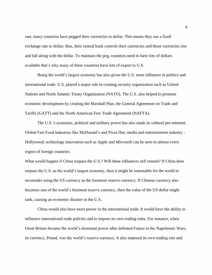
Being the world’s largest economy has also given the U.S. more influence in politics and

international trade. U.S. played a major role in creating security organization such as United

Nations and North Atlantic Treaty Organization (NATO). The U.S. also helped to promote

economic development by creating the Marshall Plan, the General Agreement on Trade and

Tariffs (GATT) and the North American Free Trade Agreement (NAFTA).

The U.S.’s economic, political and military power has also made its cultural pre-eminent.

Global Fast Food industries like McDonald’s and Pizza Hut; media and entertainment industry -

Hollywood; technology innovation such as Apple and Microsoft can be seen in almost every

region of foreign countries.

What would happen if China surpass the U.S.? Will these influences still remain? If China does

surpass the U.S. as the world’s largest economy, then it might be reasonable for the world to

reconsider using the US currency as the foremost reserve currency. If Chinese currency also

becomes one of the world’s foremost reserve currency, then the value of the US dollar might

tank, causing an economic disaster in the U.S.

China would also have more power in the international trade. It would have the ability to

influence international trade policies and to impose its own trading rules. For instance, when

Great Britain became the world’s dominant power after defeated France in the Napoleonic Wars,

its currency, Pound, was the world’s reserve currency. It also imposed its own trading rule and

https://www.thebalance.com/facts-about-nafta-statistics-and-accomplishments-3306280

9

forced Chinese market open to opium and when China refused, Great Britain launched into wars

and Great Britain also discriminated against Indian textile production.

Chinese culture is one of world’s oldest culture and has been considered the dominance

culture in East Asia, originated more than 5000 years ago. Its language, ceramics, calligraphy,

cuisine, martial arts, dance have a profound impact on the world. When China has more global

economic and political influence, it’s very likely that the world would become more influence by

its cultural; especially with the help of its huge population, approximately 1.4 billion of people

and the many more Chinese immigrates spread around the world.

Despite China being an emerging country, it has risen to the world’s second largest

economy, right after the U.S (Focus Economic, 2018). This paper will be comparing the

economic growth in U.S. and China, the world’s 1st and 2nd largest economies in term of GDP in

the period of 1982-2016. It will examine the following question:

Will Chinese economy surpass the U.S. economy in the next 20 years in terms of its GDP

per capita?

Unit Root Test-Phillips Perron (PP) will be used to check the stationarity of each

variable. Granger Causality Test will be used to analyze the relationship between variables. VAR

models will be used for forecasting the economic growth in China and U.S. in the next 20 years.

The structure of the paper is as follows: Part II is the literature review, Part III is the

model, description of variables, and data description, Part IV shows the results from regression

analysis, Part V is the forecasting and Part VI is the conclusion.

10

Chapter 2. Literature Review

Saving

Theoretical literature is unclear about the direction of causality between saving rate and

growth and the relationship between saving and growth. The early growth model of Harrod and

Domar (1939; 1946), Y=AK stated that output (Y) is proportional to capital (K) where A is a

constant. With capital as the only factor in the model and constant marginal returns to capital,

this model shows that output growth rate would be proportional to saving rate or investment. In

other models, labors are also included but since in developing counties like Bangladesh and

China where there are surplus of labors, growth would be proportional to saving rate that’s why

Lewis (1954) believed that higher saving can lead to faster economic growth. Solow’s model

(1956) assumed decreasing marginal return to capital lead to growth eventually stop but

economies with higher saving rate can have higher steady state income (Agrawal, 2001).

Assuming diminishing return to capital makes sense since adding more capital makes output

increasing in a decreasing rate. For example, if a firm gets a unit of capital, a computer, the

output can increase, but if this firm keeps adding more computers without adding more labors,

the growth in output will gradually stops. Recent growth model by Romer (1986) agreed with

Harrod and Domar’s assumption of constant return to capital and believed that higher saving rate

and capital formation lead to higher output growth rate (Agrawal, 2011).

Consumption theories like permanent income and life cycle hypotheses implied opposite

direction of causality between saving and growth. People choose their consumption and saving

based on their current and future level of income. According to Modigliani (1970), life cycle

hypothesis showed a positive relationship between saving and growth in income. He argued that

with no growth in income and population, saving of the young would cancel out the dissaving of

11

the old, therefore aggregate saving would be zero. But increase in income for young people make

them richer than the old people, so young people would save more than the amount not saved by

the old people, it showed a positive relationship between saving and growth. However, Carroll

and Weil (1994) argued that, ceteris paribus, an exogenous increase in aggregate growth will

make forward looking consumers feel wealthier and which lead to an increase in consumption,

therefore less saving, which means the relationship between growth and saving can also be

negative if consumption habit change with an increase in income (Agrawal, 2001).

The empirical work on the causality between saving rate and growth is also ambiguous.

Agrawal used Granger causality analysis testing seven Asian countries using modern time series

analysis. He chose East Asian countries because these countries are among the highest saving

and growth rate in the world. After analyzing the behaviors of saving rate and growth in seven

Asian countries, he found that high rate of growth in income per capital do lead to high saving

rate in six out of seven East Asian countries. But in three countries, higher saving rate led to

higher growth rate. However, the result is much stronger from growth to saving than the other

way around. Saltz (1999) used vector error correction (VEC) and vector auto regression (VAR)

to look at the relationship between saving and economic growth in 17 countries. The finding was

ambiguous. In 2 countries, domestic saving was the cause of economic growth, but in 9

countries, economic growth was the cause of an increase in domestic saving, and in 3 countries,

they found no causal relationship between the 2 variables. In the last 2 countries, they found a 2-

way causal relationship between domestic saving and economic growth, meaning domestic

saving was the cause of economic growth and economic growth was the cause of domestic

saving. Caroll and Weil (1994) used five-year average rate of economic growth in OECD

countries and found economic growth was a cause of saving by using Granger Causality test but

12

was questioned by others and these people believed that if they used annual data instead then the

causal relationship would be reversed. Misztal (2011) used co-integration and Granger causality

test to analyze the relationship between domestic saving and economic growth in developing,

emerging and developed countries. He used both Keynes model, saving is a function of

economic growth and Solow hypothesis, saving is a determinant of economic growth. After

looking at the correlation coefficient, Granger test and co-integration in both advanced countries

and emerging and developing countries, Misztal found one-way, positive relationship between

domestic saving in both advanced countries and emerging and developing countries, meaning

gross domestic saving was the cause of GDP but not the other way around. This result is

consistent with Solow hypothesis. And he concluded that the level of economic development in

the countries is not important when looking at the relationship between saving and development.

Krieckhaus (2002) used 32 countries in his research and found that higher domestic saving can

cause an increase in investment and therefore cause an increase in economic growth. Katircioglu

and Naraliyeva (2006) used Granger causality test and cointegration method to find the

relationship between FDI, domestic saving and economic growth in Kazakhstan in the period of

1993-2002 and found a one-way, positive relationship between domestic saving and economic

growth.

Trade

Many researchers believed that international trade was the main reason why East Asian

countries were growing rapidly in the past years (Balassa,1971; Krueger, 1993; and Hughes,

1992). According to Zestos and Tao, countries participate in international trade for several

reasons. First, by increasing export sectors, countries can achieve economies of scale. Exporting

goods allows countries to increase production. Trade also allows countries to specialize in certain

13

production which they have the lowest opportunity cost, in other words, comparative advantage.

It is especially true for small countries where markets are too small for specialization. Second,

trade promotes higher efficiency. It gives workers higher wage and firms, higher profit because

only the most efficient companies can survive in the competitive international market. Trade also

allows different products to come to the host country which means variety of selection are

available to consumers, thus consumers can get higher quality products. Third, trade allows host

countries to have access to higher level of technology. This is especially true to developing

countries. Also importing similar products from foreign countries can encourage innovation.

Competitive pressure from foreign opponent is important for growth (Jomo et al, 2001). On the

other hand, countries that are against international trade argued that trade cannot increase

productivity growth in countries due to lack of skills to make it work. For many developing

countries, using a more advanced technology requires some training, a certain level of human

capital and without having the skills to run these technologies, developing countries cannot gain

much through trade. Other opponents of international trade pointed out that if developing

countries have industries that are pretty new, then these infant industries would not be able to

compete and survive in the international competition, thus these infant industries need to be

protected. Furthermore, industries should be protected from dumping. Dumping occurs when

manufacturers export products at a price that is lower in the foreign importing market than the

price in the exporter’s domestic market, often times because they have excess supply of certain

product. Dumping can cause a big decline in the market price and thus drive other industries out

of business. Friedrich List and Joseph Stiglitz are the few economists that are against free trade.

Zestos and Tao used 49 observations and looked at the causal relationship between trade

and GDP growth in 2 countries: Canada and United States. They found that from period of 1948-

14

1996, Canada’s economy has always been more open than the United States’. In 1996, total trade

as a percentage of GDP for Canada was approximately 80% compared to approximately 25% for

the U.S. (Zestos and Tao, 2002). After using Granger Causality test, Cointegration and Vector

Error Correction model, they concluded that Canadian GDP is closely related with both the

export and import. They believed that the reason why import was related to GDP growth was

because Canadian mainly imported new technology and some other manufacturing products such

as tools or machinery and these goods tend to help industrialize and contribute to the growth of

the domestic economy. Canadian’s export were mainly natural resources and by engaging in

exporting, they got the foreign exchange they needed to pay for its imports. In contrast, for the

U.S, even though the export and GDP were positive correlated, imports and GDP were not.

Some of the explanations were the U.S. has been a major industrial country for a long time and

they don’t rely on imported technology and physical capitals to grow. Its large national market

made it possible to be economically separated from the rest of the world. The U.S. was able to

import goods and invest in foreign market regardless of its export level, so it made its import and

export not so closely related, unlike other countries who have to export because it provides the

required foreign currency to pay for their imports. Another explanation for the weaker Granger

causality in the U.S. is that the U.S. government deficit since the early 1980s caused higher

interest rate, which attracted foreign financial capital to the U.S. (Zestos and Tao).

FDI

FDI can facilitate host country’s economic development by increase in capital formation,

employment creation, knowledge spillovers and transfer technology. This view was supported by

several others. Chen (2011) found that FDI has helped China’s economic growth directly through

increasing in capital inputs and indirectly through positive knowledge spillovers. Dees (1998)

15

also supported this idea that FDI affected China’s economic growth from spread of knowledge

and ideas. Whalley and Xin found that China’s foreign-invested corporations contributed more

than 40% of its economic growth in the period of 2003-2004 and without FDI, its GDP growth

rate might be about 3.4% points less (Whalley and Xing, 2010). According to the United Nations

Conference on Trade and Development (UNCTAD), by the end of 2016, China attracted $1.35

trillion in FDI, making it the largest FDI recipient in the developing world. Policy change

regarding FDI in China made attracting FDI possible.

According to the author of China’s 40 Years of Reform and Development, Chunlai Chen

in 1975, Deng Xiaoping, the Chinese former Chairman, commissioned the drafting of a

document about “Four Modernizations”, which is the modernization of agriculture, industry,

science & technology and national defense, he strongly believed that by achieving these

modernization would be crucial to China’s economic development, and wanted to acquire

advanced technology and management skills from foreign countries. However, these ideas were

being fiercely attacked and he was being labeled as “capitalist” and removed from government

party. But when he returned to office again in 1978, he reintroduced these ideas again and by

seeing how other developing countries use FDI to facilitate their economic development and

what FDI did to these countries, Chinese leaders started to realize the importance of FDI and

believed it is an effective way to obtain advanced technology from foreign countries at the

minimum cost. With the abundant of supplies of labors, FDI helped to better allocate Chinese

resources. Eagerness of wanting to recover from economic disruption caused by Cultural

Revolution and desperate demand for economic growth promoted initial changes to China’s

policies regarding FDI.

16

Growth of FDI in China can be divided into three phases: the first phase, 1979-1991; the

second phase, 1992-2001 and the third phase, 2002-2017 (Chen, 2018).

The First Phase:

After the open-door policy in 1978, China opened four special economic zones, aka

SEZs- Shenzhen, Zhuhai, Xiamen and Shantou in 1980. During this period, the Chinese

government putted in a lot of effort to liberalize FDI policies and encourage FDI inflows, they

did so by opening more areas to FDI and offering special tax incentives to foreign investors and

introducing series of laws and regulation to attract FDI. However, the uneven implementing of

FDI policies made coastal cities gained more benefit compared to inland, therefore, the gap in

economic development and income level encouraged those skilled workers, capital and technical

personnel to move to coastal region from inland (Chen, 2017). During this first phase, China was

cautious about bring FDI into its country, so did the investors, so FDI inflow was about $1.8

billion annually.

The Second Phase:

After Deng Xiaoping visited DEZs and some other costal economical opened areas, he

wanted to implement FDI policies nationwide. Chinese government implemented new regulation

and policies that would further encourage FDI by opening 52 cities to foreign investors, granted

14 more coastal cities the preferential policies and declared 15 border cities and counties as

open-border cities (Chen, 2018). Besides, China also established more duty-free zones and

allowed foreign investors purchase land use rights for the building of infrastructure facilities

(Wei, 1994). Wanting to expedite economic growth and close economic growth gap between

coastal and inland region, in 1998, Chinese government also launched the West Development

Strategy which covered 12 provinces, municipalities and autonomous regions (Garnaut et al,

17

2018). According to Chen, during this phase, due to the more systematic and consistent FDI

regulatory framework, inflow of FDI in 1992 doubled from the previous year and reached

$11billion, and it doubled again in 1993 reached $27.5 billion. However, due to the Est Asian

Financial Crisis, it slowed after 1997 and declined in 1999.

The Third Phase:

This phase began a year after China joined World Trade Organization (WTO) in 2001.

After joining WTO, China amended more laws and issued more regulation to fulfill its

commitments to WTO and for foreign investors to acquire China’s domestic business. In 2002,

China issued the Provisions on Guiding the Orientation of Foreign Investment and divided FDI

into four categories: “encouraged”, “permitted”, “restricted” and “prohibited” to guide FDI

inflows to targeted economic industries. Industries under “restricted” category were subjected to

controls and limitation and these under “prohibited” categories were completely closed to FDI.

In 2007, Chinese lawmakers unified tax rates for domestic and foreign companies and this new

tax rate was 25%. In this phase, FDI increased to $108.3 billion in 2008 from $46.9 billion in

2001 (Chen, 2018).

According to Chen, at the end of 2014, the top 15 investors in China accounted for 87.5%

of total FDI inflows in China, they were Hong Kong (China), 46.5%; British Virgin Islands, 8.8);

Japan, 6.1%; the United States, 4.7%; Singapore, 45%; Taiwan (China), 3.8%; South Korea,

3.7%; Cayman Islands, 1.8%; Germany, 1.5%; Samoa, 1.5%; the United Kingdom, 1.2%;

Netherlands, 0.9%; France, 0.9%; Mauritius 0.8%; and Macau (China); 0.7%. Also, developing

economies accounted for 68.7% of FDI inflows in China, followed by 18.09% from developed

economies. Tax haven or countries that have low tax rate accounted for 13.1% of total FDI.

18

Chen (2018) also talked about how FDI contributed to China’s economic growth through four

channels. First, FDI caused a higher demand for labor thus, created employment and increase in

total output, therefore boosted its economic growth. FDI also increased China’s fixed capital

formation through its FDI attraction. Moreover, FDI is the leading source for technology transfer

for developing countries so it is expected to increase China’s economic growth. Lastly, FDI can

cause knowledge spillovers, so it is expected to accelerate Chinese firm’s efficiency and

productivity.

19

Chapter 3. Data and Methodology

Data Description

All data were obtained from the World Bank’s World Development Indicator (WDI).

Data for FDI was available in the period of 1982-2017 for China and 1970-2017 for U.S. Data on

gross saving rate was available in the period of 1982-2017 for China and 1970-2016 for U.S.

Data on gross capital formation and how much products were imported and the total amount of

goods that were exported were available for both countries since 1960, but up to 2016 for U.S.

and 2017 for China. Data on GDP per capita growth in both counties were available from 1961

to 2017 and data on population growth rate in both countries were available in the period of

1960-2017. R&D would be an important variable that can influence economic growth since

technology affects economic growth in the long run, but unfortunately almost all R&D related

data for China were unavailable and the earliest available R&D data for China, Researchers in

R&D (per million people) didn’t start until 1996. Since at least 30 number of observations would

be needed to run regression analysis and get accurate results, despite the importance of R&D, it

has to be excluded in this paper. The fact that all the data were available in both countries since

1982 and the data for saving, trade and capital formation were available up to 2016 for the U.S.,

resulted this paper will consist 35 number of observations (1982-2016). Table 1 provides a

description of the variables used in the model.

20

Variable Description

Table 1

List of Variables

Variables Description

Capital (K) Gross fixed capital formation (% of GDP)

Labor (L) Population growth (annual %) as a proxy for

labor participation rate

Savings (S) Gross savings (% of GDP)

Openness to trade (Trade) Summation of Exports of goods and services

(% of GDP) and Imports of goods and

services (% of GDP)

Foreign direct investment (FDI) Foreign direct investment, net inflows (% of

GDP)

GDP per capita (Y) Constant (or real) GDP per capita, 2010 U.S.

dollars

LY log (Y)

LY (-1) log (Y) lagged in 1 period, or last year GDP

per capita

Methodology

Cobb-Douglas production function is widely used to represent the relationship between

the two inputs, capital and labor and the amount of output that can be produced using these

inputs. It states that dependent variable Y is the function of independent variables K and L.

Cobb-Douglas production function:

General form: Y=F (K, L)

Specific form: Y= A Kα L β where 0 < α and β < 1

21

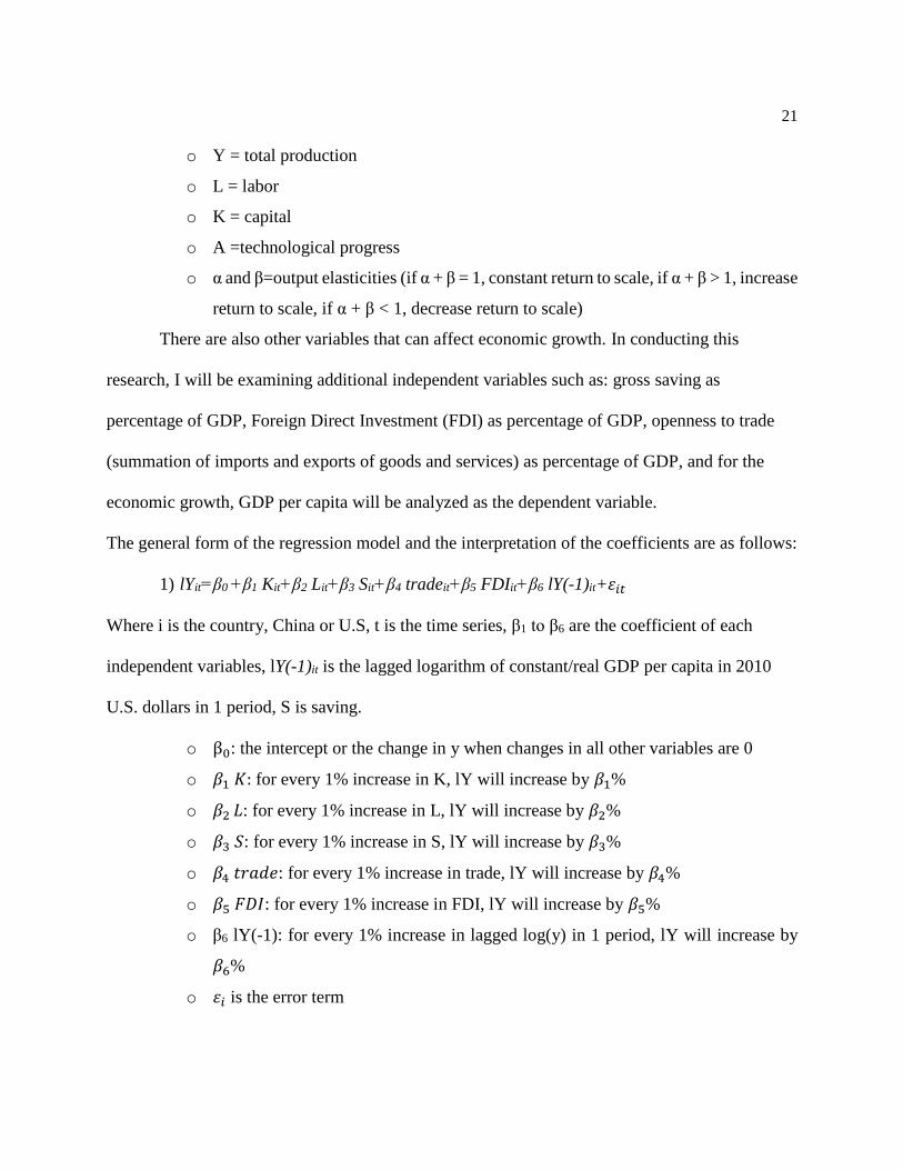
o Y = total production

o L = labor

o K = capital

o A =technological progress

o α and β=output elasticities (if α + β = 1, constant return to scale, if α + β > 1, increase

return to scale, if α + β < 1, decrease return to scale)

There are also other variables that can affect economic growth. In conducting this

research, I will be examining additional independent variables such as: gross saving as

percentage of GDP, Foreign Direct Investment (FDI) as percentage of GDP, openness to trade

(summation of imports and exports of goods and services) as percentage of GDP, and for the

economic growth, GDP per capita will be analyzed as the dependent variable.

The general form of the regression model and the interpretation of the coefficients are as follows:

1) lYit=β0 +β1 Kit+β2 Lit+β3 Sit+β4 tradeit+β5 FDIit+β6 lY(-1)it+𝜀𝑖𝑡

Where i is the country, China or U.S, t is the time series, β1 to β6 are the coefficient of each

independent variables, lY(-1)it is the lagged logarithm of constant/real GDP per capita in 2010

U.S. dollars in 1 period, S is saving.

o β0: the intercept or the change in y when changes in all other variables are 0

o 𝛽1 𝐾: for every 1% increase in K, lY will increase by 𝛽1%

o 𝛽2 𝐿: for every 1% increase in L, lY will increase by 𝛽2%

o 𝛽3 𝑆: for every 1% increase in S, lY will increase by 𝛽3%

o 𝛽4 𝑡𝑟𝑎𝑑𝑒: for every 1% increase in trade, lY will increase by 𝛽4%

o 𝛽5 𝐹𝐷𝐼: for every 1% increase in FDI, lY will increase by 𝛽5%

o β6 lY(-1): for every 1% increase in lagged log(y) in 1 period, lY will increase by

𝛽6%

o 𝜀𝑖 is the error term

https://en.wikipedia.org/wiki/Labour_(economics)

https://en.wikipedia.org/wiki/Capital_(economics)

https://en.wikipedia.org/wiki/Output_elasticity

22

Unit Rroot-Phillips Perron. It is well known that if a chosen variable shows unit roots,

it would violate classical econometrics, the presence of a unit root implies that a shock today has

a long-lasting impact (Wooldridge, 2016), thus using procedures of classical econometrics would

not be appropriate. Therefore, in order to estimate the model, we need to first check the

stationarity of the chosen variables. Unit Root Test Phillips-Perron (1988) will be used to check

the stationarity of each variable. A series is said to be stationary if the mean and autocovariances

of the series do not depend on time. Any series that is not stationary is said to be nonstationary

(Eviews user’s guide).

One hypothesis is being tested:

The null hypothesis (H0): variable is non-stationary, or it has unit root, (p = 1)

The alternative hypothesis (H1): variable is stationary, or it has no unit root), (p < 1)

H0 will be rejected if |tc|>|critical value|, meaning variable has no unit root, therefore it is

stationary.

H0 will be failed to reject if |tc|<|critical value|, meaning variable has unit root, therefore it

is non-stationary.

Granger causality test. Granger causality is a way to investigate causal relation between

two variables in a time series (Granger, 1969). A time series X is said to granger cause Y if the

past value of X or lagged value of X provide statistically significant information and help to

predict future values of Y and this prediction is based on the knowledge of past values of Y alone

(Zestos and Tao, 2011). Pairwise causality test is the standard causality test that is a bidirectional

test for Granger Causality between 2 variables. It shows the directional relationship between 2

variables, for instance, whether X causes Y or Y causes X.

One hypothesis is being tested:

23

The null hypothesis (H0): X does not granger cause/effect Y (or Y does not granger cause

X)

The alternative hypothesis (H1): X does granger cause Y (or Y does granger cause X)

F statistics or p-value is being used to test Null hypothesis. AIC will be used to determine the

number of lags included in the model.

H0 will be rejected if p-value < 5%, meaning X does granger cause or effect Y

H0 will be failed to reject if p-value > 5%, meaning X does not granger cause or effect Y.

Vector Autoregression (VAR). The vector autoregression (VAR), a multivariate

regression is commonly used for forecasting systems of interrelated time series and for analyzing

the dynamic impact of random disturbances on the system of variables (Eviews). It treats every

endogenous variable in the system as a function of p-lagged values of all of the endogenous

variables in the system. In other words, in each equation, we regress the left-hand-side variable

on p lags of itself, and p lags of every other variable, so the right-hand-side variables are the

same in every equation, p lags of every variable. In VAR, each variable is not just related to its

own past, but also to the past of all the other variables in the system (Diebold, 2017).

In the five-variable VAR (3), we have:

2) lY it=Φ11 lY it-1+Φ12 K it-1+ Φ13 Lit-1+ Φ14 Sit-1+ Φ15 tradeit-1+ Φ16 FDIit-1+Φ17 lY it-

2+Φ18 K it-2+ Φ19 Lit-2+ Φ20 Sit-2+ Φ21 tradeit-2+ Φ22 FDIit-2 + Φ23 lY it-3+Φ24 K it-3+

Φ25 Lit-3+ Φ26 Sit-3+ Φ27 Tradeit-3+ Φ28 FDIit-3 𝜀1,𝑖𝑡

3) K it=Φ11 lY it-1+Φ12 K it-1+ Φ13 Lit-1+ Φ14 Sit-1+ Φ15 tradeit-1+ Φ16 FDIit-1+Φ17 lY it-



24

4) L it=Φ11 lY it-1+Φ12 K it-1+ Φ13 Lit-1+ Φ14 Sit-1+ Φ15 tradeit-1+ Φ16 FDIit-1+Φ17 lY it-



5) S it=Φ11 lY it-1+Φ12 K it-1+ Φ13 Lit-1+ Φ14 Sit-1+ Φ15 tradeit-1+ Φ16 FDIit-1+Φ17 lY it-



6) Trade it=Φ11 lY it-1+Φ12 K it-1+ Φ13 Lit-1+ Φ14 Sit-1+ Φ15 tradeit-1+ Φ16 FDIit-1+Φ17 lY it-



7) FDI it=Φ11 lY it-1+Φ12 K it-1+ Φ13 Lit-1+ Φ14 Sit-1+ Φ15 tradeit-1+ Φ16 FDIit-1+Φ17 lY it-



Where i is the country: China or U.S., t is the time series, Φ# is the coefficient of each

endogenous variables and 𝜀 is the error term in each equation

In the above models, each variable depends on 3 lags of the other variable other than 3

lags of itself; which can be useful in forecasting. Order (3) is being selected because AIC is

minimized.

25

Chapter 4 Test results

Unit Root Test

China.

Null Hypothesis: LCHINA_Y has a unit root

Exogenous: None

Bandwidth: 2 (Newey-West automatic) using Bartlett kernel

Adj. t-Stat Prob.*

Phillips-Perron test statistic 12.69164 1.0000

Test critical values: 1% level -2.634731

5% level -1.951000

10% level -1.610907

*MacKinnon (1996) one-sided p-values.

Residual variance (no correction) 0.000742

HAC corrected variance (Bartlett kernel) 0.001433

Figure 1: Phillips-Perron Unit Root Test on LChina_Y

Phillips-Perron statistic value is 12.69164 and one sided p-value is 1.0000. Based on the

critical values provided at 1%, 5% and 10% levels, the calculated t value is greater than the

critical value, thus we reject the null hypothesis LChina_Y has a unit root or LChina_Y is non-

stationary, meaning LChina_Y has no unit root and it is stationary.

Null Hypothesis: CHINA_K has a unit root

Exogenous: None


Adj. t-Stat Prob.*



5% level -1.951000

10% level -1.610907




Figure 2: Phillips-Perron Unit Root Test on China_K

26



absolute critical value at 10%, thus we reject the null hypothesis China_K has a unit root or

China_K is non-stationary, meaning China_K has no unit root therefore it is stationary.

Null Hypothesis: CHINA_L has a unit root

Exogenous: None


Adj. t-Stat Prob.*

Phillips-Perron test statistic -2.255924 0.0252


5% level -1.951000

10% level -1.610907




Figure 3: Phillips-Perron Unit Root Test on China_L

Phillips-Perron statistic value is -2.255924 and one sided p-value is 0.0252. Based on the

critical values provided at 1%, 5% and 10% levels, the calculated t value in absolute term is

greater than the absolute critical value at both 5% and 10%, thus we reject the null hypothesis

China_L has a unit root or China_L is non-stationary, meaning China_L has no unit root

therefore it is stationary.

Null Hypothesis: CHINA_S has a unit root

27

Exogenous: None


Adj. t-Stat Prob.*



5% level -1.951000

10% level -1.610907




Figure 4: Phillips-Perron Unit Root Test on China_S


critical values provided at 1%, 5% and 10% levels, the calculated t value is not greater than any

absolute critical value, thus we failed to reject the null hypothesis China_S has a unit root or

China_S is non-stationary, meaning China_S has a unit root therefore it is non-stationary.

Null Hypothesis: CHINA_TRADE has a unit root

Exogenous: None


Adj. t-Stat Prob.*



5% level -1.951000

10% level -1.610907




Figure 5: Phillips-Perron Unit Root Test on China_Trade



28

absolute critical value, thus we failed to reject the null hypothesis China_Trade has a unit root or

China_Trade is non-stationary, meaning China_Trade has a unit root therefore it is non-

stationary.

Null Hypothesis: CHINA_FDI has a unit root

Exogenous: None


Adj. t-Stat Prob.*



5% level -1.951000

10% level -1.610907




Figure 6: Phillips-Perron Unit Root Test on China_FDI


critical values provided at 1%, 5% and 10% levels, the calculated t value in absolute term is not

greater than any absolute critical value, thus we failed to reject the null hypothesis China_FDI

has a unit root or China_FDI is non-stationary, meaning China_FDI has a unit root therefore it is

non-stationary.

Because variables China_S, China_Trade and China_FDI are non-stationary, 1st

differencing will be used to check for stationarity.

Null Hypothesis: D(CHINA_S) has a unit root

Exogenous: None


Adj. t-Stat Prob.*

29



5% level -1.951332

10% level -1.610747




Figure 7: Phillips-Perron Unit Root Test on D(China_S)



greater than absolute critical value, thus we reject the null hypothesis D(China_S) has a unit root

or D(China_S) is non-stationary, meaning D(China_S) has no unit root therefore it is stationary.

Null Hypothesis: D(CHINA_TRADE) has a unit root

Exogenous: None


Adj. t-Stat Prob.*



5% level -1.951332

10% level -1.610747




Figure 8: Phillips-Perron Unit Root Test on D(China_Trade)



greater than absolute critical value, thus we reject the null hypothesis D(China_Trade) has a unit

30

root or D(China_Trade) is non-stationary, meaning D(China_Trade) has no unit root therefore it

is stationary.

Null Hypothesis: D(DCHINA_FDI) has a unit root

Exogenous: None


Adj. t-Stat Prob.*



5% level -1.951687

10% level -1.610579




Figure 9: Phillips-Perron Unit Root Test on D(China_FDI)



greater than absolute critical value, thus we reject the null hypothesis D(China_FDI) has a unit

root or D(China_FDI) is non-stationary, meaning D(China_FDI) has no unit root therefore it is

stationary.

Since the 1st difference of variables China_S, China_Trade and China_FDI are stationary,

D(China_S), D(China_Trade) and D(China_FDI) will be used in the OLS regression for China

model.

31

U.S.

Null Hypothesis: LUS_Y has a unit root

Exogenous: None


Adj. t-Stat Prob.*



5% level -1.951000

10% level -1.610907




Figure 10: Phillips-Perron Unit Root Test on LUS_Y



critical value, thus we reject the null hypothesis LUS_Y has a unit root or LUS_Y is non-

stationary, meaning LUS_Y has no unit root therefore it is stationary.

Null Hypothesis: US_K has a unit root

Exogenous: None


Adj. t-Stat Prob.*



5% level -1.951000

10% level -1.610907




Figure 11: Phillips-Perron Unit Root Test on US_K

32



greater than any absolute critical value, thus we failed to reject the null hypothesis US_K has a

unit root or US_K is non-stationary, meaning US_K has a unit root therefore it is non-stationary.

Null Hypothesis: US_L has a unit root

Exogenous: None


Adj. t-Stat Prob.*



5% level -1.951000

10% level -1.610907




Figure 12: Phillips-Perron Unit Root Test on US_L



greater than any absolute critical value, thus we failed to reject the null hypothesis US_L has a

unit root or US_L is non-stationary, meaning US_L has a unit root therefore it is non-stationary.

33

Null Hypothesis: US_S has a unit root

Exogenous: None


Adj. t-Stat Prob.*



5% level -1.951000

10% level -1.610907




Figure 13: Phillips-Perron Unit Root Test on US_S



greater than any absolute critical value, thus we failed to reject the null hypothesis US_S has a

unit root or US_S is non-stationary, meaning US_S has a unit root therefore it is non-stationary.

Null Hypothesis: US_TRADE has a unit root

Exogenous: None


Adj. t-Stat Prob.*



5% level -1.951000

10% level -1.610907




Figure 14: Phillips-Perron Unit Root Test on US_Trade



34

greater than any absolute critical value, thus we failed to reject the null hypothesis US_Trade has

a unit root or US_Trade is non-stationary, meaning US_Trade has a unit root therefore it is non-

stationary.

Null Hypothesis: US_FDI has a unit root

Exogenous: None


Adj. t-Stat Prob.*



5% level -1.951000

10% level -1.610907




Figure 15: Phillips-Perron Unit Root Test on US_FDI



absolute critical value, thus we failed to reject the null hypothesis US_FDI has a unit root or

US_FDI is non-stationary, meaning US_FDI has a unit root therefore it is non-stationary.

Since all the variables are non-stationary except for LUS_Y, 1st differencing of these non-

stationary variables will be used to check for stationarity.

35

Null Hypothesis: D(US_K) has a unit root

Exogenous: None


Adj. t-Stat Prob.*



5% level -1.951332

10% level -1.610747




Figure 16: Phillips-Perron Unit Root Test on D(US_K)



greater than absolute critical value at both 5% and 10%, thus we reject the null hypothesis D

(US_K) has a unit root or D(US_K) is non-stationary, meaning D(US_K) has no unit root

therefore it is stationary.

Null Hypothesis: D(US_L) has a unit root

Exogenous: None


Adj. t-Stat Prob.*



5% level -1.951332

10% level -1.610747




Figure 17: Phillips-Perron Unit Root Test on D(US_L)

36



greater than absolute critical value, thus we reject the null hypothesis D(US_L) has a unit root or

D(US_L) is non-stationary, meaning D(US_L) has no unit root therefore it is stationary.

Null Hypothesis: D(US_S) has a unit root

Exogenous: None


Adj. t-Stat Prob.*



5% level -1.951332

10% level -1.610747




Figure 18: Phillips-Perron Unit Root Test on D(US_S)



greater than absolute critical value, thus we reject the null hypothesis D(US_S) has a unit root or

D(US_S) is non-stationary, meaning D(US_S) has no unit root therefore it is stationary.

37

Null Hypothesis: D(US_TRADE) has a unit root

Exogenous: None


Adj. t-Stat Prob.*



5% level -1.951332

10% level -1.610747




Figure 19: Phillips-Perron Unit Root Test on D(US_Trade)



greater than absolute critical value, thus we reject the null hypothesis D(US_Trade) has a unit

root or D(US_Trade) is non-stationary, meaning D(US_Trade) has no unit root therefore it is

stationary.

Null Hypothesis: D(US_FDI) has a unit root

Exogenous: None


Adj. t-Stat Prob.*



5% level -1.951332

10% level -1.610747




Figure 20: Phillips-Perron Unit Root Test on D(US_FDI)

38



greater than absolute critical value, thus we reject the null hypothesis D(US_FDI) has a unit root

or D(US_FDI) is non-stationary, meaning D(US_FDI) has no unit root therefore it is stationary.

Since the 1st difference of variables US_K, US_L, US_S, US_Trade and US_FDI are stationary,

D(US_K), D(US_L), D(US_S), D(US_Trade) and D(US_FDI) will be used in the OLS

regression for U.S. model.

Ordinary Least Square (OLS) Regression Results

China.

LChina_Y = 0.404933369153 + 0.00432475183731*China_K - 0.0597125396966*China_L +

0.00397961292061*DChina_S - 0.000368030530241*DChina_Trade +

0.00267408727574*DChina_FDI + 0.942709693083*LChina_Y(-1)

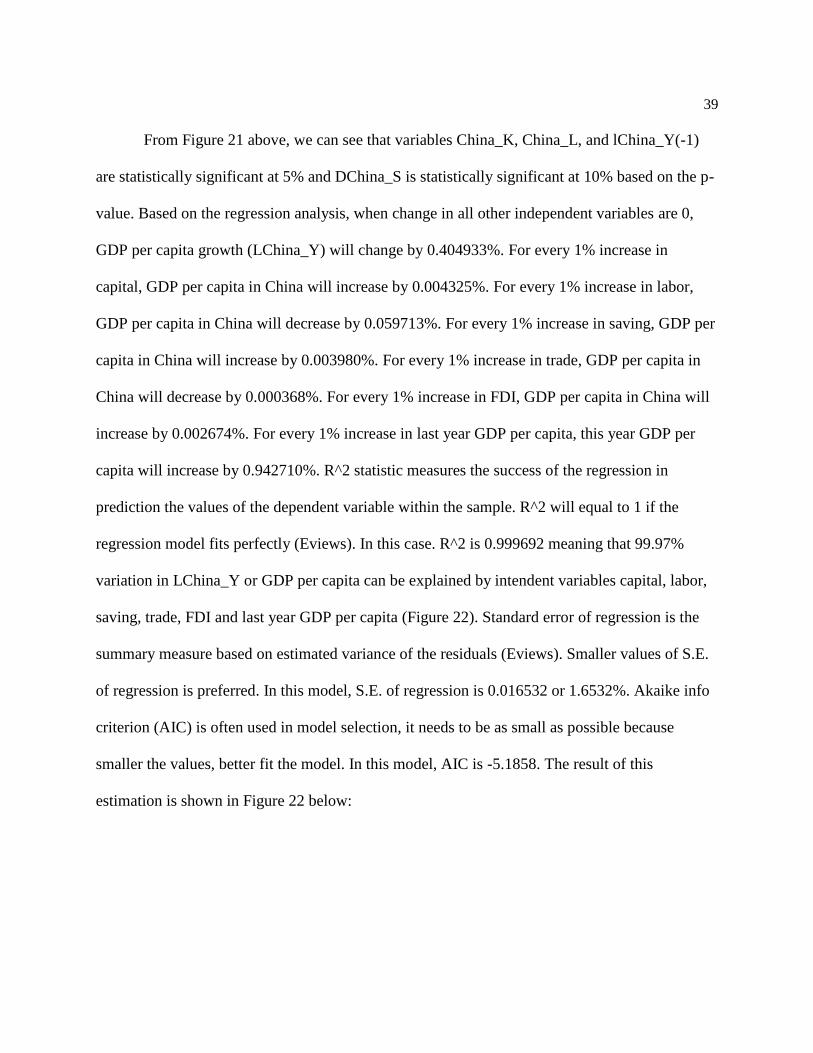
Dependent Variable: LCHINA_Y

Method: Least Squares

Sample (adjusted): 1983 2016

Included observations: 34 after adjustments

Variable Coefficient Std. Error t-Statistic Prob.

C 0.404933 0.101485 3.990084 0.0005

CHINA_K 0.004325 0.001178 3.671334 0.0010

CHINA_L -0.059713 0.023498 -2.541170 0.0171

DCHINA_S 0.003980 0.002310 1.722962 0.0963

DCHINA_TRADE -0.000368 0.000916 -0.401868 0.6909

DCHINA_FDI 0.002674 0.004298 0.622197 0.5390

LCHINA_Y(-1) 0.942710 0.012337 76.41059 0.0000

R-squared 0.999692 Mean dependent var 7.474667

Adjusted R-squared 0.999624 S.D. dependent var 0.852334

S.E. of regression 0.016532 Akaike info criterion -5.185838

Sum squared resid 0.007379 Schwarz criterion -4.871587

Log likelihood 95.15924 Hannan-Quinn criter. -5.078669

F-statistic 14615.58 Durbin-Watson stat 1.398982

Prob(F-statistic) 0.000000

Figure 21: OLS Regression for China

39

From Figure 21 above, we can see that variables China_K, China_L, and lChina_Y(-1)

are statistically significant at 5% and DChina_S is statistically significant at 10% based on the p-

value. Based on the regression analysis, when change in all other independent variables are 0,

GDP per capita growth (LChina_Y) will change by 0.404933%. For every 1% increase in

capital, GDP per capita in China will increase by 0.004325%. For every 1% increase in labor,

GDP per capita in China will decrease by 0.059713%. For every 1% increase in saving, GDP per

capita in China will increase by 0.003980%. For every 1% increase in trade, GDP per capita in

China will decrease by 0.000368%. For every 1% increase in FDI, GDP per capita in China will

increase by 0.002674%. For every 1% increase in last year GDP per capita, this year GDP per

capita will increase by 0.942710%. R^2 statistic measures the success of the regression in

prediction the values of the dependent variable within the sample. R^2 will equal to 1 if the

regression model fits perfectly (Eviews). In this case. R^2 is 0.999692 meaning that 99.97%

variation in LChina_Y or GDP per capita can be explained by intendent variables capital, labor,

saving, trade, FDI and last year GDP per capita (Figure 22). Standard error of regression is the

summary measure based on estimated variance of the residuals (Eviews). Smaller values of S.E.

of regression is preferred. In this model, S.E. of regression is 0.016532 or 1.6532%. Akaike info

criterion (AIC) is often used in model selection, it needs to be as small as possible because

smaller the values, better fit the model. In this model, AIC is -5.1858. The result of this

estimation is shown in Figure 22 below:

40

-.04

-.02

.00

.02

.04

6.0

6.5

7.0

7.5

8.0

8.5

9.0

1985 1990 1995 2000 2005 2010 2015

Residual Actual Fitted

Figure 22: Actual, Fitted, Residual graph-China

U.S.

LUS_Y = 0.507575727447 + 0.0142110607548*D(US_K) - 0.0285837840245*D(US_L) -

0.000299043169509*D(US_S) + 0.000583814796331*D(US_Trade) +

0.00614646491008*D(US_FDI) + 0.953976981603*LUS_Y(-1)

41

Dependent Variable: LUS_Y

Method: Least Squares



Variable Coefficient Std. Error t-Statistic Prob.

C 0.507576 0.087040 5.831505 0.0000

D(US_K) 0.014211 0.002674 5.313766 0.0000

D(US_L) -0.028584 0.021561 -1.325696 0.1960

D(US_S) -0.000299 0.001494 -0.200192 0.8428

D(US_TRADE) 0.000584 0.001032 0.565492 0.5764

D(US_FDI) 0.006146 0.002725 2.255279 0.0324

LUS_Y(-1) 0.953977 0.008195 116.4088 0.0000

R-squared 0.998151 Mean dependent var 10.64519

Adjusted R-squared 0.997740 S.D. dependent var 0.168396

S.E. of regression 0.008005 Akaike info criterion -6.636155

Sum squared resid 0.001730 Schwarz criterion -6.321904

Log likelihood 119.8146 Hannan-Quinn criter. -6.528986

F-statistic 2429.140 Durbin-Watson stat 1.712421

Prob(F-statistic) 0.000000

Figure 23: OLS Regression for U.S.

From Figure 23 above, we can see that variables D(US_K), D(US_FDI), and LUS_Y(-1)

are statistically significant at 5% based on the p-value. Based on the regression analysis, when

change in all other independent variables are 0, GDP per capita growth (LUS_Y) will change by

0.507576%. For every 1% increase in capital, GDP per capita in China will increase by

0.014211%. For every 1% increase in labor, GDP per capita in China will decrease by 0.028584.

For every 1% increase in saving, GDP per capita in China will decrease by 0.000299. For every

1% increase in trade, GDP per capita in China will increase by 0.000584%. For every 1%

increase in FDI, GDP per capita in China will increase by 0.006146%. For every 1% increase in

last year GDP per capita, this year GDP per capita will increase by 0.953977%. R^2 is 0.998151

meaning that 99.82% variation in LUS_Y or GDP per capita can be explained by intendent

variables capital, labor, saving, trade, FDI and last year GDP per capita (Figure 24). In this U.S.

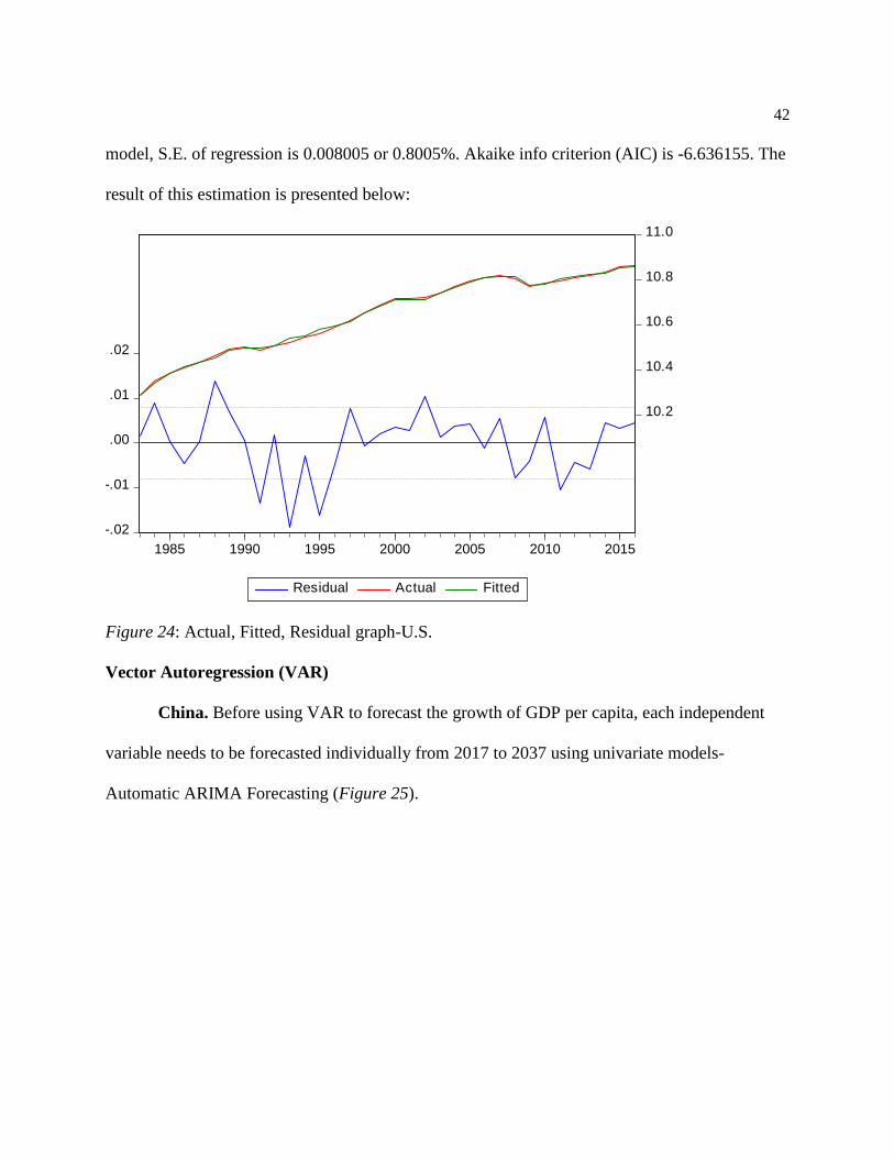
42

model, S.E. of regression is 0.008005 or 0.8005%. Akaike info criterion (AIC) is -6.636155. The

result of this estimation is presented below:

-.02

-.01

.00

.01

.02

10.2

10.4

10.6

10.8

11.0

1985 1990 1995 2000 2005 2010 2015

Residual Actual Fitted

Figure 24: Actual, Fitted, Residual graph-U.S.

Vector Autoregression (VAR)

China. Before using VAR to forecast the growth of GDP per capita, each independent

variable needs to be forecasted individually from 2017 to 2037 using univariate models-

Automatic ARIMA Forecasting (Figure 25).

43

Figure a: Automatic ARIMA Forecasting-capital

Figure b: Automatic ARIMA Forecasting-labor

-15

-10

-5

0

5

10

2005 2010 2015 2020 2025 2030 2035

Forecast Actual

Actual and Forecast

Figure c: Automatic ARIMA Forecasting-Trade

-1.2

-0.8

-0.4

0.0

0.4

0.8

1.2

1.6

2005 2010 2015 2020 2025 2030 2035

Forecast Actual

Actual and Forecast

Figure d: Automatic ARIMA Forecasting-FDIq

Figure e: Automatic ARIMA Forecasting-S

Figure 25: Automatic ARIMA forecasting for each variable

44

Table 2 provides the Automatic ARIMA forecasting for each variable in China during the

period of 2017 to 2037.

Table 2

Automatic ARIMA Forecasting for each Variable - China

Year K L S Trade FDI

2017 53.25342 0.560261 0.646162 -10.8916 -0.62937

2018 54.71409 0.565967 0.646162 -5.35498 0.808162

2019 56.21858 0.574072 0.646162 -7.65659 -0.53051

2020 57.76689 0.583197 0.646162 -8.9229 -1.52466

2021 59.35902 0.593827 0.646162 -6.59502 -0.83672

2022 60.99496 0.602325 0.646162 -6.33634 -0.6159

2023 62.67472 0.595805 0.646162 -7.92129 -0.84485

2024 64.3983 0.571657 0.646162 -5.14439 -0.58515

2025 66.1657 0.540857 0.646162 -4.12075 -0.36751

2026 67.97692 0.515303 0.646162 -5.02299 -0.45338

2027 69.83195 0.493204 0.646162 -5.97799 -0.755

2028 71.7308 0.468313 0.646162 -5.80141 -0.8053

2029 73.67347 0.443909 0.646162 -5.39416 -0.62411

2030 75.65995 0.424921 0.646162 -4.9529 -0.57898

2031 77.69026 0.408554 0.646162 -4.65915 -0.71562

2032 79.76438 0.391238 0.646162 -4.63989 -0.75598

2033 81.88232 0.37466 0.646162 -5.03695 -0.70936

2034 84.04407 0.359758 0.646162 -5.29722 -0.72444

2035 86.24965 0.343969 0.646162 -5.15048 -0.74742

2036 88.49904 0.3273 0.646162 -5.03312 -0.68997

2037 90.79225 0.313455 0.646162 -5.25968 -0.65716

VAR result – China. After forecasting each independent variable individually from

period 2017-2037 using the univariate models-Automatic ARIMA, VAR can be used to forecast

the growth of GDP per capita. VAR gets the best result using 3 lags in this model.

45

Vector Autoregression Estimates



Standard errors in ( ) & t-statistics in [ ]

LCHINA_Y CHINA_K CHINA_L DCHINA_S

DCHINA_TRA

DE DCHINA_FDI

LCHINA_Y(-1) 1.562787 30.58983 -0.070558 -13.06959 -51.31473 21.74305

(0.24073) (34.3725) (0.47275) (25.7032) (51.0797) (11.4095)

[ 6.49199] [ 0.88995] [-0.14925] [-0.50848] [-1.00460] [ 1.90570]

LCHINA_Y(-2) -1.313247 -25.43024 0.515548 -45.10676 -164.7801 -48.78044

(0.35433) (50.5933) (0.69584) (37.8329) (75.1848) (16.7938)

[-3.70632] [-0.50264] [ 0.74090] [-1.19226] [-2.19167] [-2.90467]

LCHINA_Y(-3) 0.728091 5.975677 -0.428718 49.14440 186.4742 26.92600

(0.20691) (29.5435) (0.40633) (22.0922) (43.9035) (9.80658)

[ 3.51894] [ 0.20227] [-1.05509] [ 2.22451] [ 4.24736] [ 2.74571]

CHINA_K(-1) -0.001250 0.358465 0.000487 0.024470 0.794226 0.173555

(0.00256) (0.36573) (0.00503) (0.27349) (0.54350) (0.12140)

[-0.48796] [ 0.98014] [ 0.09691] [ 0.08947] [ 1.46133] [ 1.42963]

CHINA_K(-2) -0.003505 -0.378160 0.003976 -0.163183 0.638363 0.026249

(0.00254) (0.36250) (0.00499) (0.27107) (0.53870) (0.12033)

[-1.38061] [-1.04320] [ 0.79753] [-0.60199] [ 1.18501] [ 0.21815]

CHINA_K(-3) 0.000577 -0.353660 -0.001290 0.370891 -0.347409 -0.058893

(0.00237) (0.33861) (0.00466) (0.25321) (0.50320) (0.11240)

[ 0.24344] [-1.04444] [-0.27702] [ 1.46475] [-0.69040] [-0.52397]

CHINA_L(-1) 0.130648 34.86050 2.005399 -11.70603 -50.67458 -2.199638

(0.15439) (22.0453) (0.30320) (16.4851) (32.7606) (7.31763)

[ 0.84621] [ 1.58132] [ 6.61403] [-0.71010] [-1.54681] [-0.30059]

CHINA_L(-2) -0.246706 -49.53028 -1.536091 5.970469 50.95461 0.169632

(0.19078) (27.2406) (0.37466) (20.3701) (40.4813) (9.04216)

[-1.29316] [-1.81825] [-4.09997] [ 0.29310] [ 1.25872] [ 0.01876]

CHINA_L(-3) 0.002939 17.69254 0.589470 -9.158171 -40.86787 5.081405

(0.10236) (14.6158) (0.20102) (10.9295) (21.7200) (4.85153)

[ 0.02871] [ 1.21051] [ 2.93238] [-0.83793] [-1.88158] [ 1.04738]

DCHINA_S(-1) 9.24E-05 0.164590 -4.78E-05 0.225385 -0.031406 0.134467

(0.00302) (0.43082) (0.00593) (0.32216) (0.64022) (0.14300)

[ 0.03062] [ 0.38204] [-0.00807] [ 0.69961] [-0.04905] [ 0.94030]

DCHINA_S(-2) -0.001418 0.240955 0.002046 0.027571 -0.209037 -0.040700

(0.00256) (0.36520) (0.00502) (0.27309) (0.54271) (0.12122)

[-0.55457] [ 0.65979] [ 0.40730] [ 0.10096] [-0.38517] [-0.33574]

DCHINA_S(-3) 0.007090 0.288826 0.001189 0.143171 -0.123494 0.199995

(0.00275) (0.39300) (0.00541) (0.29388) (0.58402) (0.13045)

[ 2.57608] [ 0.73493] [ 0.21989] [ 0.48718] [-0.21146] [ 1.53312]

46

DCHINA_TRADE(-1) -0.001351 0.059568 -0.000334 -0.176913 -0.364817 -0.072378

(0.00126) (0.17935) (0.00247) (0.13412) (0.26653) (0.05953)

[-1.07560] [ 0.33213] [-0.13525] [-1.31910] [-1.36877] [-1.21576]

DCHINA_TRADE(-2) 0.000196 -0.045616 0.001589 0.080285 0.006012 0.090593

(0.00103) (0.14679) (0.00202) (0.10976) (0.21813) (0.04872)

[ 0.19020] [-0.31077] [ 0.78720] [ 0.73143] [ 0.02756] [ 1.85932]

DCHINA_TRADE(-3) -0.000992 -0.115103 -0.001814 -0.051513 -0.149898 -0.028237

(0.00115) (0.16360) (0.00225) (0.12234) (0.24313) (0.05431)

[-0.86593] [-0.70355] [-0.80627] [-0.42106] [-0.61655] [-0.51997]

DCHINA_FDI(-1) 0.011459 -0.275612 0.002780 1.077751 1.318046 -0.324209

(0.00634) (0.90597) (0.01246) (0.67747) (1.34632) (0.30072)

[ 1.80606] [-0.30422] [ 0.22310] [ 1.59085] [ 0.97900] [-1.07810]

DCHINA_FDI(-2) 0.007050 -0.208719 -0.021089 0.021522 -0.217726 -0.659938

(0.00479) (0.68435) (0.00941) (0.51175) (1.01699) (0.22716)

[ 1.47101] [-0.30499] [-2.24056] [ 0.04206] [-0.21409] [-2.90514]

DCHINA_FDI(-3) 0.007521 0.578654 0.005376 0.209563 1.212778 -0.078012

(0.00538) (0.76812) (0.01056) (0.57439) (1.14147) (0.25497)

[ 1.39800] [ 0.75334] [ 0.50890] [ 0.36485] [ 1.06247] [-0.30597]

C 0.520518 -37.60620 -0.340146 78.26918 239.4548 -6.927899

(0.31130) (44.4497) (0.61135) (33.2388) (66.0551) (14.7545)

[ 1.67207] [-0.84604] [-0.55639] [ 2.35475] [ 3.62508] [-0.46954]

R-squared 0.999868 0.956306 0.997970 0.665266 0.817701 0.769261

Adj. R-squared 0.999669 0.890764 0.994925 0.163165 0.544252 0.423151

Sum sq. resids 0.002432 49.58356 0.009379 27.72625 109.4995 5.463221

S.E. equation 0.014236 2.032723 0.027957 1.520040 3.020754 0.674736

F-statistic 5031.469 14.59082 327.7421 1.324966 2.990328 2.222595

Log likelihood 102.5350 -51.26701 81.61289 -42.25717 -63.54705 -17.07989

Akaike AIC -5.389354 4.533356 -4.039541 3.952076 5.325616 2.327735

Schwarz SC -4.510459 5.412251 -3.160646 4.830971 6.204511 3.206630

Mean dependent 7.600778 36.81606 0.875276 0.338538 0.526483 0.033080

S.D. dependent 0.782242 6.150286 0.392446 1.661633 4.474589 0.888388

Determinant resid covariance (dof adj.) 3.50E-07

Determinant resid covariance 1.18E-09

Log likelihood 54.76386

Akaike information criterion 3.821686

Schwarz criterion 9.095059

Number of coefficients 114

Figure 26: VAR estimation - China

Error terms can also be called innovations, impulses and shocks and impulse response

function is a shock to a VAR system. It identifies the responsiveness of the endogenous variable

47

in VAR when 1 standard deviation or 1 unit of shock is applied to an error term. In impulse

response function, all variables are assumed to be endogenous and it allows us to see the effect

on VAR when a unit of shock is applied to each variable (Hossain Academy).

As shown in Figure 27 and Figure 39, when one unit of shock is applied to capital (K) or

when K increases by one basis point, the growth of GDP per capita in China doesn’t change

much in both short-run and long-run. When one shock is applied to labor (L) or when L increases

by one basis point, the growth of GDP per capita increases marginally in the short-run, the first 4

years; but then it decreases in the long-run. It is consistent with the negative coefficient of labor

in the OLS regression for China (Figure 21). When 1 standard deviation is given to saving, the

growth of GDP per capita decreases marginal in the short-run, the first 2 or 3 years, then

increases at a decreasing rate in the long-run. For every unit of shock applied to trade, the growth

of GDP per capita decreases in a decreasing rate in both short-run and long-run then eventually

grow marginally above 0%. When 1 shock is applied to FDI, the growth of GDP per capita

increases in a decreasing rate in both short-run and long-run and eventually growth close to 0%.

48

Impulse Response Function

-.08

-.04

.00

1 2 3 4 5 6 7 8 9 10

R espons e of LCH IN A_Y to LCH INA_Y

-.08

-.04

.00

1 2 3 4 5 6 7 8 9 10

R espons e of LCH IN A_Y to C H IN A_K

-.08

-.04

.00

1 2 3 4 5 6 7 8 9 10

R espons e of LCH IN A_Y to C H IN A_L

-.08

-.04

.00

1 2 3 4 5 6 7 8 9 10

R espons e of LCH IN A_Y to D CH INA_S

-.08

-.04

.00

1 2 3 4 5 6 7 8 9 10

R es pons e of LCH IN A_Y to D CHINA_TRADE

-.08

-.04

.00

1 2 3 4 5 6 7 8 9 10

R esponse of LCH IN A_Y to D CH INA_FDI

-2

-1

0

1

2

1 2 3 4 5 6 7 8 9 10

R espons e of C HINA_K to LCH IN A_Y

-2

-1

0

1

2

1 2 3 4 5 6 7 8 9 10

R es ponse of C H IN A_K to C H IN A_K

-2

-1

0

1

2

1 2 3 4 5 6 7 8 9 10

R es ponse of C H IN A_K to C H IN A_L

-2

-1

0

1

2

1 2 3 4 5 6 7 8 9 10

R es ponse of C H IN A_K to D CH IN A_S

-2

-1

0

1

2

1 2 3 4 5 6 7 8 9 10

R es pons e of C HINA_K to D CHINA_TRADE

-2

-1

0

1

2

1 2 3 4 5 6 7 8 9 10

R esponse of C HINA_K to D CH IN A_FDI

-.1

.0

.1

.2

1 2 3 4 5 6 7 8 9 10

R espons e of C HINA_L to LCH IN A_Y

-.1

.0

.1

.2

1 2 3 4 5 6 7 8 9 10

R es ponse of C H IN A_L to C H IN A_K

-.1

.0

.1

.2

1 2 3 4 5 6 7 8 9 10

R es ponse of C H IN A_L to C H IN A_L

-.1

.0

.1

.2

1 2 3 4 5 6 7 8 9 10

R es ponse of C H IN A_L to D CH IN A_S

-.1

.0

.1

.2

1 2 3 4 5 6 7 8 9 10

R es pons e of C HINA_L to D CHINA_TRADE

-.1

.0

.1

.2

1 2 3 4 5 6 7 8 9 10

R esponse of C HINA_L to D CH IN A_FDI

-2

-1

0

1

1 2 3 4 5 6 7 8 9 10

R espons e of D CH IN A_S to LCH INA_Y

-2

-1

0

1

1 2 3 4 5 6 7 8 9 10

R es ponse of D C HIN A_S to C H IN A_K

-2

-1

0

1

1 2 3 4 5 6 7 8 9 10

R es ponse of D C HIN A_S to C H IN A_L

-2

-1

0

1

1 2 3 4 5 6 7 8 9 10

R espons e of D CH IN A_S to D CH INA_S

-2

-1

0

1

1 2 3 4 5 6 7 8 9 10

R es pons e of D CH IN A_S to D CHINA_TRADE

-2

-1

0

1

1 2 3 4 5 6 7 8 9 10

R esponse of D CH IN A_S to D CH INA_FDI

-4

-2

0

2

1 2 3 4 5 6 7 8 9 10

R es pons e of D CH IN A_TRADE to LCHINA_Y

-4

-2

0

2

1 2 3 4 5 6 7 8 9 10

R es pons e of D CH IN A_TR AD E to C HINA_K

-4

-2

0

2

1 2 3 4 5 6 7 8 9 10

R es pons e of D CH IN A_TR AD E to C HINA_L

-4

-2

0

2

1 2 3 4 5 6 7 8 9 10

R es pons e of D CH IN A_TRADE to D CHINA_S

-4

-2

0

2

1 2 3 4 5 6 7 8 9 10

R es ponse of D CHINA_TR ADE to D CHINA_TR AD E

-4

-2

0

2

1 2 3 4 5 6 7 8 9 10

R es ponse of D CHIN A_TRADE to D CHINA_FDI

-.5

.0

.5

1 2 3 4 5 6 7 8 9 10

R esponse of D CH IN A_FD I to LC HINA_Y

-.5

.0

.5

1 2 3 4 5 6 7 8 9 10

R esponse of D CH IN A_FDI to C H INA_K

-.5

.0

.5

1 2 3 4 5 6 7 8 9 10

R esponse of D CH IN A_FDI to C HINA_L

-.5

.0

.5

1 2 3 4 5 6 7 8 9 10

R esponse of D CH IN A_FD I to D C HINA_S

-.5

.0

.5

1 2 3 4 5 6 7 8 9 10

R es ponse of D CHIN A_FDI to D CHIN A_TRADE

-.5

.0

.5

1 2 3 4 5 6 7 8 9 10

R es pons e of D CH IN A_FDI to D CHINA_FDI

Response to Cholesky One S.D. (d.f. adjusted) Innovations ± 2 S.E.

Figure 27: Impulse Response Function- Response to Cholesky One S.D. Innovations +/- 2 S.E -

China

Table 3 provides the forecasting for the growth of GDP per capita in China during the

period 2017-2037 using VAR model.

49

Table 3

VAR Forecasting - LChina_Y

Year LChina_y

2017 8.89707

2018 8.949625

2019 8.997909

2020 9.03837

2021 9.073511

2022 9.107739

2023 9.141434

2024 9.172424

2025 9.20167

2026 9.231328

2027 9.261102

2028 9.289626

2029 9.317516

2030 9.345693

2031 9.373399

2032 9.400007

2033 9.426513

2034 9.453649

2035 9.480768

2036 9.507409

2037 9.533988

Table 4 provides the forecasting for variables capital, labor, saving, trade and FDI in

2017-2037 using multivariate model-VAR.

50

Table 4

VAR Forecasting-China

Year K L S Trade FDI lChina_Y

2017 45.95783 0.507654 -3.15049 -4.45677 -0.22614 8.89707

2018 45.76182 0.510132 -3.31313 -5.26402 -0.54502 8.949625

2019 45.7374 0.511696 -3.67928 -5.77726 -0.69084 8.997909

2020 45.87083 0.511018 -4.01998 -6.15163 -0.63848 9.03837

2021 45.99804 0.509797 -4.27191 -6.13687 -0.60648 9.073511

2022 46.09868 0.505029 -4.3349 -5.3978 -0.62575 9.107739

2023 46.26279 0.494772 -4.48229 -5.16345 -0.61336 9.141434

2024 46.3513 0.482589 -4.63634 -5.47776 -0.5769 9.172424

2025 46.36265 0.47068 -4.71726 -5.73706 -0.6332 9.20167

2026 46.48395 0.456898 -4.72649 -5.6075 -0.69231 9.231328

2027 46.7737 0.441046 -4.78574 -5.49422 -0.65641 9.261102

2028 47.04352 0.426236 -4.86735 -5.56006 -0.62459 9.289626

2029 47.2006 0.413364 -4.90102 -5.55265 -0.6795 9.317516

2030 47.33979 0.400526 -4.89595 -5.42054 -0.72905 9.345693

2031 47.51379 0.387441 -4.91228 -5.46214 -0.71711 9.373399

2032 47.6723 0.375348 -4.93103 -5.64038 -0.71371 9.400007

2033 47.82965 0.363763 -4.92464 -5.6673 -0.74551 9.426513

2034 48.04602 0.351493 -4.92442 -5.58154 -0.75049 9.453649

2035 48.28813 0.339341 -4.95936 -5.63631 -0.72632 9.480768

2036 48.48252 0.328692 -5.00085 -5.7978 -0.73547 9.507409

2037 48.6476 0.319198 -5.02965 -5.88679 -0.77447 9.533988

51

Figure 28 presents the forecasting graph for all the variables in China using VAR.

43

44

45

46

47

48

49

12 14 16 18 20 22 24 26 28 30 32 34 36

CHINA_K_F

.30

.35

.40

.45

.50

.55

12 14 16 18 20 22 24 26 28 30 32 34 36

CHINA_L_F

-1.4

-1.2

-1.0

-0.8

-0.6

-0.4

-0.2

0.0

12 14 16 18 20 22 24 26 28 30 32 34 36

DCHINA_FDI_F

-6

-5

-4

-3

-2

-1

0

12 14 16 18 20 22 24 26 28 30 32 34 36

DCHINA_S_F

-8

-6

-4

-2

0

2

4

12 14 16 18 20 22 24 26 28 30 32 34 36

DCHINA_TRADE_F

8.4

8.6

8.8

9.0

9.2

9.4

9.6

12 14 16 18 20 22 24 26 28 30 32 34 36

LCHINA_Y_F

Figure 28: VAR forecasting graph – China

52

Figure 29 provides the summary table for VAR forecasting evaluation in China. This

summary table includes Root Mean Square Error (RMSE), Mean Absolute Error (MAE), Mean

Absolute Percentage Error (MAPE) and Theil inequality coefficient (Theil).

Forecast Evaluation

Sample: 2011 2037

Included observations: 27

Variable Inc. obs. RMSE MAE MAPE Theil

CHINA_K 6 1.688344 1.444355 3.242232 0.018961

CHINA_L 6 0.022707 0.021589 4.174450 0.022312

DCHINA_FDI 6 0.313410 0.254487 152.3514 0.273818

DCHINA_S 6 0.990150 0.802811 64.68835 0.333869

DCHINA_TRADE 6 1.949306 1.785903 43.14058 0.264595

LCHINA_Y 6 0.001438 0.000905 0.010491 8.28E-05

RMSE: Root Mean Square Error

MAE: Mean Absolute Error

MAPE: Mean Absolute Percentage Error

Theil: Theil inequality coefficient

Figure 29: VAR forecasting evaluation – China

U.S. The graph for each independent variable forecasting using univariate models-

Automatic ARIMA from 2017 to 2037 can be seen below (Figure 30).

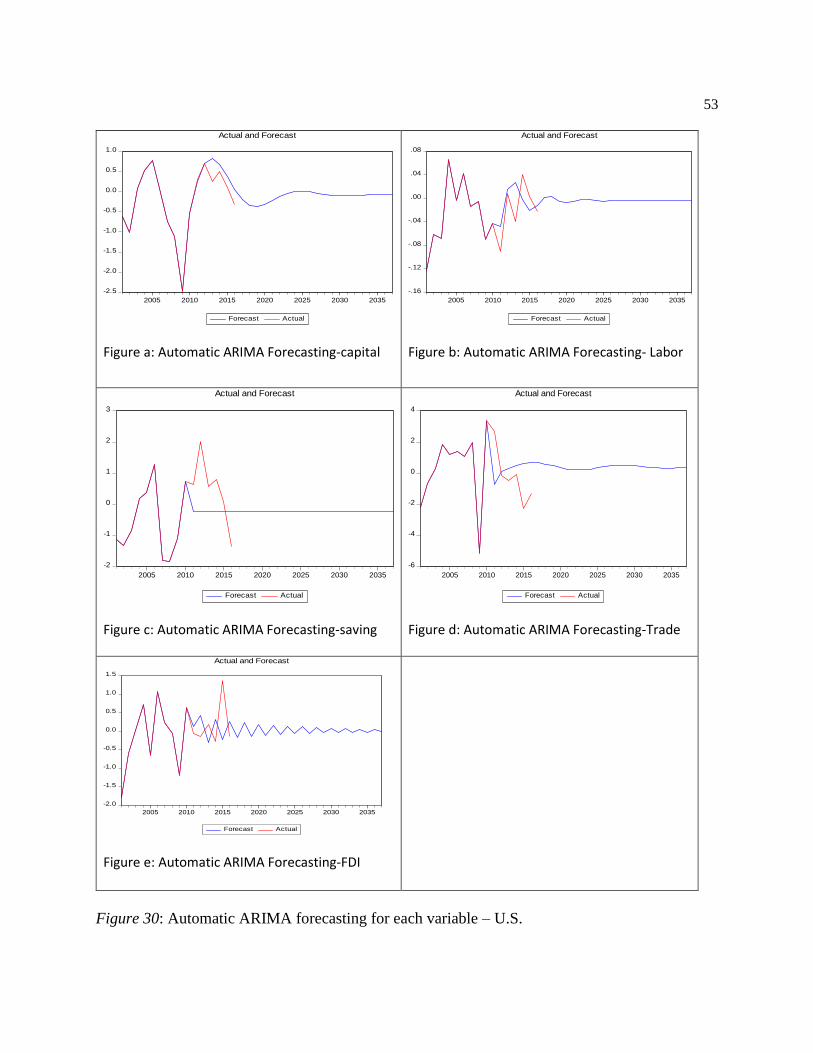
53

-2.5

-2.0

-1.5

-1.0

-0.5

0.0

0.5

1.0

2005 2010 2015 2020 2025 2030 2035

Forecast Actual

Actual and Forecast

Figure a: Automatic ARIMA Forecasting-capital

-.16

-.12

-.08

-.04

.00

.04

.08

2005 2010 2015 2020 2025 2030 2035

Forecast Actual

Actual and Forecast

Figure b: Automatic ARIMA Forecasting- Labor

-2

-1

0

1

2

3

2005 2010 2015 2020 2025 2030 2035

Forecast Actual

Actual and Forecast

Figure c: Automatic ARIMA Forecasting-saving

-6

-4

-2

0

2

4

2005 2010 2015 2020 2025 2030 2035

Forecast Actual

Actual and Forecast

Figure d: Automatic ARIMA Forecasting-Trade

-2.0

-1.5

-1.0

-0.5

0.0

0.5

1.0

1.5

2005 2010 2015 2020 2025 2030 2035

Forecast Actual

Actual and Forecast

Figure e: Automatic ARIMA Forecasting-FDI

Figure 30: Automatic ARIMA forecasting for each variable – U.S.

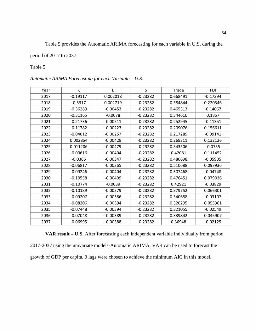
54

Table 5 provides the Automatic ARIMA forecasting for each variable in U.S. during the

period of 2017 to 2037.

Table 5

Automatic ARIMA Forecasting for each Variable – U.S.

Year K L S Trade FDI

2017 -0.19117 0.002018 -0.23282 0.668491 -0.17394

2018 -0.3317 0.002719 -0.23282 0.584844 0.220346

2019 -0.36289 -0.00453 -0.23282 0.465313 -0.14067

2020 -0.31165 -0.0078 -0.23282 0.344616 0.1857

2021 -0.21736 -0.00511 -0.23282 0.252945 -0.11351

2022 -0.11782 -0.00223 -0.23282 0.209076 0.156611

2023 -0.04012 -0.00257 -0.23282 0.217289 -0.09141

2024 0.002854 -0.00429 -0.23282 0.268311 0.132126

2025 0.011206 -0.00479 -0.23282 0.343506 -0.0735

2026 -0.00616 -0.00404 -0.23282 0.42081 0.111452

2027 -0.0366 -0.00347 -0.23282 0.480698 -0.05905

2028 -0.06817 -0.00365 -0.23282 0.510688 0.093936

2029 -0.09246 -0.00404 -0.23282 0.507468 -0.04748

2030 -0.10558 -0.00409 -0.23282 0.476451 0.079036

2031 -0.10774 -0.0039 -0.23282 0.42921 -0.03829

2032 -0.10189 -0.00379 -0.23282 0.379752 0.066301

2033 -0.09207 -0.00386 -0.23282 0.340688 -0.03107

2034 -0.08206 -0.00394 -0.23282 0.320295 0.055361

2035 -0.07448 -0.00394 -0.23282 0.321055 -0.02549

2036 -0.07048 -0.00389 -0.23282 0.339842 0.045907

2037 -0.06995 -0.00388 -0.23282 0.36948 -0.02125

VAR result – U.S. After forecasting each independent variable individually from period

2017-2037 using the univariate models-Automatic ARIMA, VAR can be used to forecast the

growth of GDP per capita. 3 lags were chosen to achieve the minimum AIC in this model.

55

Vector Autoregression Estimates



Standard errors in ( ) & t-statistics in [ ]

LUS_Y DUS_K DUS_L DUS_S DUS_TRADE DUS_FDI

LUS_Y(-1) 0.965770 -1.601031 1.441563 -20.88491 8.984832 -8.025883

(0.38327) (14.3231) (1.87951) (23.2899) (51.8962) (21.4148)

[ 2.51982] [-0.11178] [ 0.76699] [-0.89674] [ 0.17313] [-0.37478]

LUS_Y(-2) 0.169117 -15.50974 2.263729 -9.004342 24.32398 17.60754

(0.60441) (22.5874) (2.96396) (36.7279) (81.8397) (33.7709)

[ 0.27980] [-0.68665] [ 0.76375] [-0.24516] [ 0.29721] [ 0.52138]

LUS_Y(-3) -0.178459 15.83263 -3.662017 25.70339 -34.21965 -9.677405

(0.39520) (14.7689) (1.93800) (24.0147) (53.5113) (22.0813)

[-0.45157] [ 1.07202] [-1.88958] [ 1.07032] [-0.63948] [-0.43826]

DUS_K(-1) 0.006068 0.558715 -0.061791 0.245529 -0.468460 0.675688

(0.00986) (0.36847) (0.04835) (0.59914) (1.33504) (0.55090)

[ 0.61542] [ 1.51632] [-1.27796] [ 0.40980] [-0.35090] [ 1.22652]

DUS_K(-2) -0.002523 0.293083 -0.032886 0.805707 -0.207927 -0.874128

(0.01075) (0.40158) (0.05270) (0.65298) (1.45503) (0.60041)

[-0.23482] [ 0.72982] [-0.62406] [ 1.23389] [-0.14290] [-1.45588]

DUS_K(-3) 0.004861 -0.264208 -0.029116 -0.919442 -0.123953 0.776856

(0.00696) (0.26003) (0.03412) (0.42282) (0.94215) (0.38878)

[ 0.69856] [-1.01607] [-0.85331] [-2.17456] [-0.13156] [ 1.99821]

DUS_L(-1) -0.043141 -0.879810 0.261954 -6.403708 -6.184850 1.605528

(0.04669) (1.74497) (0.22898) (2.83738) (6.32246) (2.60894)

[-0.92391] [-0.50420] [ 1.14401] [-2.25691] [-0.97824] [ 0.61539]

DUS_L(-2) 0.010704 -0.086827 0.180754 2.178735 2.696011 -1.735658

(0.05255) (1.96377) (0.25769) (3.19315) (7.11522) (2.93607)

[ 0.20370] [-0.04421] [ 0.70144] [ 0.68231] [ 0.37891] [-0.59115]

DUS_L(-3) -0.006085 -0.989386 -0.303986 -6.536003 -2.533948 2.821545

(0.04348) (1.62490) (0.21322) (2.64213) (5.88739) (2.42941)

[-0.13995] [-0.60889] [-1.42568] [-2.47376] [-0.43040] [ 1.16141]

DUS_S(-1) 0.008462 0.176811 0.020717 0.440858 0.356823 0.237694

(0.00346) (0.12935) (0.01697) (0.21032) (0.46866) (0.19339)

[ 2.44469] [ 1.36694] [ 1.22060] [ 2.09610] [ 0.76137] [ 1.22909]

DUS_S(-2) -0.000677 0.074089 0.008779 -0.353660 -0.287210 0.106016

(0.00274) (0.10231) (0.01343) (0.16636) (0.37070) (0.15297)

[-0.24718] [ 0.72415] [ 0.65388] [-2.12585] [-0.77478] [ 0.69306]

DUS_S(-3) -0.001518 -0.047416 0.018214 0.324270 -0.580803 -0.065097

(0.00297) (0.11106) (0.01457) (0.18059) (0.40240) (0.16605)

[-0.51064] [-0.42694] [ 1.24981] [ 1.79564] [-1.44336] [-0.39203]

56

DUS_TRADE(-1) -0.004682 -0.131127 0.001087 0.042061 -0.244310 -0.236993

(0.00210) (0.07847) (0.01030) (0.12759) (0.28430) (0.11732)

[-2.22983] [-1.67113] [ 0.10555] [ 0.32967] [-0.85934] [-2.02013]

DUS_TRADE(-2) -0.001710 -0.139187 0.004387 -0.170601 -0.086267 0.089623

(0.00278) (0.10406) (0.01365) (0.16920) (0.37702) (0.15557)

[-0.61410] [-1.33763] [ 0.32130] [-1.00830] [-0.22881] [ 0.57607]

DUS_TRADE(-3) -0.000982 -0.020803 0.016030 0.136192 0.739727 0.005461

(0.00241) (0.09009) (0.01182) (0.14648) (0.32641) (0.13469)

[-0.40747] [-0.23093] [ 1.35606] [ 0.92975] [ 2.26628] [ 0.04055]

DUS_FDI(-1) -0.000332 -0.095616 -0.026996 -0.232281 0.458354 -0.160968

(0.00519) (0.19395) (0.02545) (0.31537) (0.70273) (0.28998)

[-0.06399] [-0.49299] [-1.06071] [-0.73653] [ 0.65225] [-0.55510]

DUS_FDI(-2) -0.004548 -0.082232 -0.021589 0.476614 0.219862 -0.147570

(0.00573) (0.21412) (0.02810) (0.34817) (0.77581) (0.32013)

[-0.79375] [-0.38405] [-0.76837] [ 1.36893] [ 0.28340] [-0.46096]

DUS_FDI(-3) -0.009355 -0.319557 -0.065310 -0.523293 -1.914931 -0.670190

(0.00596) (0.22290) (0.02925) (0.36244) (0.80761) (0.33326)

[-1.56845] [-1.43365] [-2.23290] [-1.44381] [-2.37110] [-2.01102]

C 0.481373 13.97454 -0.567042 45.30031 8.972457 1.253447

(0.27750) (10.3706) (1.36085) (16.8629) (37.5752) (15.5053)

[ 1.73465] [ 1.34751] [-0.41668] [ 2.68639] [ 0.23879] [ 0.08084]

R-squared 0.997467 0.853410 0.747784 0.816663 0.621155 0.595147

Adj. R-squared 0.993667 0.633525 0.369460 0.541658 0.052887 -0.012132

Sum sq. resids 0.001587 2.216069 0.038159 5.859228 29.09222 4.953739

S.E. equation 0.011499 0.429735 0.056391 0.698762 1.557033 0.642504

F-statistic 262.4891 3.881162 1.976569 2.969631 1.093068 0.980023

Log likelihood 109.1535 -3.094184 59.86269 -18.16457 -43.00259 -15.56251

Akaike AIC -5.816357 1.425431 -2.636303 2.397714 4.000167 2.229839

Schwarz SC -4.937462 2.304327 -1.757407 3.276610 4.879062 3.108734

Mean dependent 10.67465 -0.133631 -0.004897 -0.074206 0.322765 0.070791

S.D. dependent 0.144494 0.709870 0.071015 1.032131 1.599915 0.638642

Determinant resid covariance (dof adj.) 2.63E-09

Determinant resid covariance 8.84E-12

Log likelihood 130.5870

Akaike information criterion -1.070127

Schwarz criterion 4.203245

Number of coefficients 114

Figure 31: VAR estimation – U.S.

As shown in Figure 32 and Figure 40, when one unit of shock is applied to capital (K),

the growth of GDP per capita in the U.S. doesn’t increase much in the first 2 years but then it

increases in a decreasing rate in the long run, compared to the response of growth of GDP per

57

capita in China for one shock in capital, which doesn’t change much in both short-run and long-

run. When one shock is applied to labor (L) or when L increases by one basis point, the growth

of GDP per capita decreases in the short-run and reach its minimum between year 4 and 5, then it

increases after year 5 and eventually approaches to 0 in the long-run. When one standard

deviation is given to saving, the growth of GDP per capita increases in a decreasing rate in the

first 3 years, and it decreases at a decreasing rate between year 4 and 5, then it increases again in

the long-run after year 5. For every unit of shock applied to trade, the growth of GDP per capita

decreases in a decreasing rate in both short-run and long-run. When one shock is applied to FDI,

the growth of GDP per capita stays the same for the first 2 years but decreases and then reaches

its minimum in year 3 and half. The growth of GDP per capita was zero in year 5 for one shock

in FDI, but then increases in a decreasing rate in the long-run.

58

Impulse Response Function

-.02

.00

.02

1 2 3 4 5 6 7 8 9 10

Response of LUS_Y to LUS_Y

-.02

.00

.02

1 2 3 4 5 6 7 8 9 10

Response of LUS_Y to DUS_K

-.02

.00

.02

1 2 3 4 5 6 7 8 9 10

Response of LUS_Y to DUS_L

-.02

.00

.02

1 2 3 4 5 6 7 8 9 10

Response of LUS_Y to DUS_S

-.02

.00

.02

1 2 3 4 5 6 7 8 9 10

Response of LUS_Y to DUS_TRADE

-.02

.00

.02

1 2 3 4 5 6 7 8 9 10

Response of LUS_Y to DUS_FDI

-.4

.0

.4

1 2 3 4 5 6 7 8 9 10

Response of DUS_K to LUS_Y

-.4

.0

.4

1 2 3 4 5 6 7 8 9 10

Response of DUS_K to DUS_K

-.4

.0

.4

1 2 3 4 5 6 7 8 9 10

Response of DUS_K to DUS_L

-.4

.0

.4

1 2 3 4 5 6 7 8 9 10

Response of DUS_K to DUS_S

-.4

.0

.4

1 2 3 4 5 6 7 8 9 10

Response of DUS_K to DUS_TRADE

-.4

.0

.4

1 2 3 4 5 6 7 8 9 10

Response of DUS_K to DUS_FDI

-.04

.00

.04

1 2 3 4 5 6 7 8 9 10

Response of DUS_L to LUS_Y

-.04

.00

.04

1 2 3 4 5 6 7 8 9 10

Response of DUS_L to DUS_K

-.04

.00

.04

1 2 3 4 5 6 7 8 9 10

Response of DUS_L to DUS_L

-.04

.00

.04

1 2 3 4 5 6 7 8 9 10

Response of DUS_L to DUS_S

-.04

.00

.04

1 2 3 4 5 6 7 8 9 10

Response of DUS_L to DUS_TRADE

-.04

.00

.04

1 2 3 4 5 6 7 8 9 10

Response of DUS_L to DUS_FDI

-.4

.0

.4

1 2 3 4 5 6 7 8 9 10

Response of DUS_S to LUS_Y

-.4

.0

.4

1 2 3 4 5 6 7 8 9 10

Response of DUS_S to DUS_K

-.4

.0

.4

1 2 3 4 5 6 7 8 9 10

Response of DUS_S to DUS_L

-.4

.0

.4

1 2 3 4 5 6 7 8 9 10

Response of DUS_S to DUS_S

-.4

.0

.4

1 2 3 4 5 6 7 8 9 10

Response of DUS_S to DUS_TRADE

-.4

.0

.4

1 2 3 4 5 6 7 8 9 10

Response of DUS_S to DUS_FDI

-1

0

1

1 2 3 4 5 6 7 8 9 10

Response of DUS_TRADE to LUS_Y

-1

0

1

1 2 3 4 5 6 7 8 9 10

Response of DUS_TRADE to DUS_K

-1

0

1

1 2 3 4 5 6 7 8 9 10

Response of DUS_TRADE to DUS_L

-1

0

1

1 2 3 4 5 6 7 8 9 10

Response of DUS_TRADE to DUS_S

-1

0

1

1 2 3 4 5 6 7 8 9 10

Response of DUS_TRADE to DUS_TRADE

-1

0

1

1 2 3 4 5 6 7 8 9 10

Response of DUS_TRADE to DUS_FDI

-.4

.0

.4

1 2 3 4 5 6 7 8 9 10

Response of DUS_FDI to LUS_Y

-.4

.0

.4

1 2 3 4 5 6 7 8 9 10

Response of DUS_FDI to DUS_K

-.4

.0

.4

1 2 3 4 5 6 7 8 9 10

Response of DUS_FDI to DUS_L

-.4

.0

.4

1 2 3 4 5 6 7 8 9 10

Response of DUS_FDI to DUS_S

-.4

.0

.4

1 2 3 4 5 6 7 8 9 10

Response of DUS_FDI to DUS_TRADE

-.4

.0

.4

1 2 3 4 5 6 7 8 9 10

Response of DUS_FDI to DUS_FDI

Response to Cholesky One S.D. (d.f. adjusted) Innovations ± 2 S.E.

Figure 32: Impulse Response Function- Response to Cholesky One S.D. Innovations +/- 2 S.E –

U.S.

Table 6 presents the forecasting for the growth of GDP per capita in U.S. during 2017-

2037 using VAR model.

59

Table 6

VAR Forecasting -LUS_Y

Year Lus_Y

2017 10.8853

2018 10.88994

2019 10.90686

2020 10.92344

2021 10.93922

2022 10.95165

2023 10.95726

2024 10.95418

2025 10.95293

2026 10.95444

2027 10.96125

2028 10.97456

2029 10.98803

2030 10.99724

2031 11.00041

2032 10.99904

2033 10.99637

2034 10.99877

2035 11.00652

2036 11.01824

2037 11.0306

Table 7 provides the forecasting for variables capital, labor, saving, trade and FDI in

2017-2037 using multivariate model-VAR

60

Table 7

VAR Forecasting- U.S.

Year K L S Trade FDI Lus_Y

2017 -0.64237 -0.14026 -0.73191 -0.03667 -0.37554 10.8853

2018 -0.68511 -0.15543 -0.64959 -2.08785 -0.66729 10.88994

2019 0.042295 -0.08003 -0.08329 0.643346 0.140341 10.90686

2020 0.510667 -0.01684 0.563189 1.212595 -0.05937 10.92344

2021 0.520467 0.018119 0.757122 -0.12742 0.051163 10.93922

2022 0.188326 -0.00966 -0.43954 -0.27678 0.305941 10.95165

2023 -0.16463 -0.03479 -1.06694 0.091289 0.216469 10.95726

2024 -0.67979 -0.09816 -1.22938 -1.12863 -0.09034 10.95418

2025 -0.73457 -0.1342 -0.94588 -0.36982 -0.33523 10.95293

2026 -0.41444 -0.13271 -0.36824 0.340211 -0.36504 10.95444

2027 -0.00443 -0.08973 0.253225 0.006171 -0.30144 10.96125

2028 0.419789 -0.03078 0.666883 0.688647 0.097435 10.97456

2029 0.53228 -0.00293 0.49842 0.621192 0.182553 10.98803

2030 0.24997 -0.01235 -0.11266 -0.30586 0.253528 10.99724

2031 -0.21708 -0.05801 -0.91231 -0.69568 0.167495 11.00041

2032 -0.53357 -0.10454 -1.11998 -0.52772 -0.0746 10.99904

2033 -0.62753 -0.1426 -0.89906 -0.75773 -0.31389 10.99637

2034 -0.34419 -0.13611 -0.35212 -0.17198 -0.32435 10.99877

2035 0.102211 -0.09682 0.248485 0.392375 -0.19654 11.00652

2036 0.420949 -0.04844 0.558238 0.310853 -0.02033 11.01824

2037 0.470714 -0.02099 0.322969 0.189588 0.206713 11.0306

Figure 33 presents the forecasting graph for all the variables in U.S. using VAR.

61

-.8

-.4

.0

.4

.8

12 14 16 18 20 22 24 26 28 30 32 34 36

DUS_FDI_F

-0.8

-0.4

0.0

0.4

0.8

1.2

12 14 16 18 20 22 24 26 28 30 32 34 36

DUS_K_F

-.16

-.12

-.08

-.04

.00

.04

12 14 16 18 20 22 24 26 28 30 32 34 36

DUS_L_F

-2

-1

0

1

2

12 14 16 18 20 22 24 26 28 30 32 34 36

DUS_S_F

-3

-2

-1

0

1

2

12 14 16 18 20 22 24 26 28 30 32 34 36

DUS_TRADE_F

10.75

10.80

10.85

10.90

10.95

11.00

11.05

12 14 16 18 20 22 24 26 28 30 32 34 36

LUS_Y_F

Figure 33: VAR forecasting – U.S.

62

Figure 34 provides the summary table for VAR forecasting evaluation in U.S. This

summary table includes Root Mean Square Error (RMSE), Mean Absolute Error (MAE), Mean

Absolute Percentage Error (MAPE) and Theil inequality coefficient (Theil).

Forecast Evaluation

Sample: 2011 2037

Included observations: 27

Variable Inc. obs. RMSE MAE MAPE Theil

DUS_FDI 6 0.456092 0.372562 108.0397 0.451448

DUS_K 6 0.266101 0.210741 35.11842 0.260781

DUS_L 6 0.048200 0.039924 271.7330 0.450421

DUS_S 6 0.398111 0.298892 35.21668 0.181517

DUS_TRADE 6 0.800981 0.721133 118.1592 0.268134

LUS_Y 6 0.013342 0.011297 0.104026 0.000616

RMSE: Root Mean Square Error

MAE: Mean Absolute Error

MAPE: Mean Absolute Percentage Error

Theil: Theil inequality coefficient

Figure 34: VAR forecasting evaluation – U.S.

Granger Causality Test

Figure 35 shows that at 5% statistics level, growth of GDP per capita (LChina_Y) in

China does not granger cause capital (K), trade and FDI (0.0079 and 0.0550, 0.0157

respectively), it just means that the directional relationship or directional effect for variables K,

trade and FDI is unidirectional from Y to capital, Y to trade and Y to FDI. Saving does not

granger cause growth of GDP per capita at 5% (0.0315) means that the directional relationship

for saving is unidirectional from saving to Y, which is consistent with the finding of Misztal

(2011) and Krieckhaus (2002), a one-way, positive relationship between domestic saving and

economic growth. Labor does not granger cause growth of GDP per capita at 10% (0.0757)

meaning that the directional relationship for labor is also unidirectional from labor to Y.

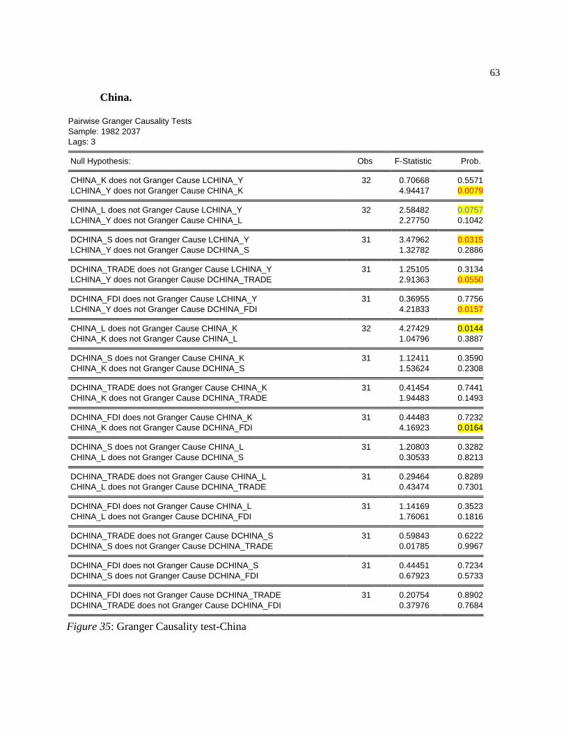
63

China.

Pairwise Granger Causality Tests

Sample: 1982 2037

Lags: 3

Null Hypothesis: Obs F-Statistic Prob.

CHINA_K does not Granger Cause LCHINA_Y 32 0.70668 0.5571

LCHINA_Y does not Granger Cause CHINA_K 4.94417 0.0079

CHINA_L does not Granger Cause LCHINA_Y 32 2.58482 0.0757

LCHINA_Y does not Granger Cause CHINA_L 2.27750 0.1042

DCHINA_S does not Granger Cause LCHINA_Y 31 3.47962 0.0315

LCHINA_Y does not Granger Cause DCHINA_S 1.32782 0.2886

DCHINA_TRADE does not Granger Cause LCHINA_Y 31 1.25105 0.3134

LCHINA_Y does not Granger Cause DCHINA_TRADE 2.91363 0.0550

DCHINA_FDI does not Granger Cause LCHINA_Y 31 0.36955 0.7756

LCHINA_Y does not Granger Cause DCHINA_FDI 4.21833 0.0157

CHINA_L does not Granger Cause CHINA_K 32 4.27429 0.0144

CHINA_K does not Granger Cause CHINA_L 1.04796 0.3887

DCHINA_S does not Granger Cause CHINA_K 31 1.12411 0.3590

CHINA_K does not Granger Cause DCHINA_S 1.53624 0.2308

DCHINA_TRADE does not Granger Cause CHINA_K 31 0.41454 0.7441

CHINA_K does not Granger Cause DCHINA_TRADE 1.94483 0.1493

DCHINA_FDI does not Granger Cause CHINA_K 31 0.44483 0.7232

CHINA_K does not Granger Cause DCHINA_FDI 4.16923 0.0164

DCHINA_S does not Granger Cause CHINA_L 31 1.20803 0.3282

CHINA_L does not Granger Cause DCHINA_S 0.30533 0.8213

DCHINA_TRADE does not Granger Cause CHINA_L 31 0.29464 0.8289

CHINA_L does not Granger Cause DCHINA_TRADE 0.43474 0.7301

DCHINA_FDI does not Granger Cause CHINA_L 31 1.14169 0.3523

CHINA_L does not Granger Cause DCHINA_FDI 1.76061 0.1816

DCHINA_TRADE does not Granger Cause DCHINA_S 31 0.59843 0.6222

DCHINA_S does not Granger Cause DCHINA_TRADE 0.01785 0.9967

DCHINA_FDI does not Granger Cause DCHINA_S 31 0.44451 0.7234

DCHINA_S does not Granger Cause DCHINA_FDI 0.67923 0.5733

DCHINA_FDI does not Granger Cause DCHINA_TRADE 31 0.20754 0.8902

DCHINA_TRADE does not Granger Cause DCHINA_FDI 0.37976 0.7684

Figure 35: Granger Causality test-China

64

Figure 36 shows that at 5% statistics level, growth of GDP per capita (LUS_Y) in the

U.S. does not granger cause capital (K), (0.0544), meaning that the directional relationship for

variables K, is unidirectional from Y to capital instead of capital to Y. Saving does not granger

cause growth of GDP per capita at 5% (0.0394) meaning that the directional relationship for

saving is also unidirectional from saving to Y.

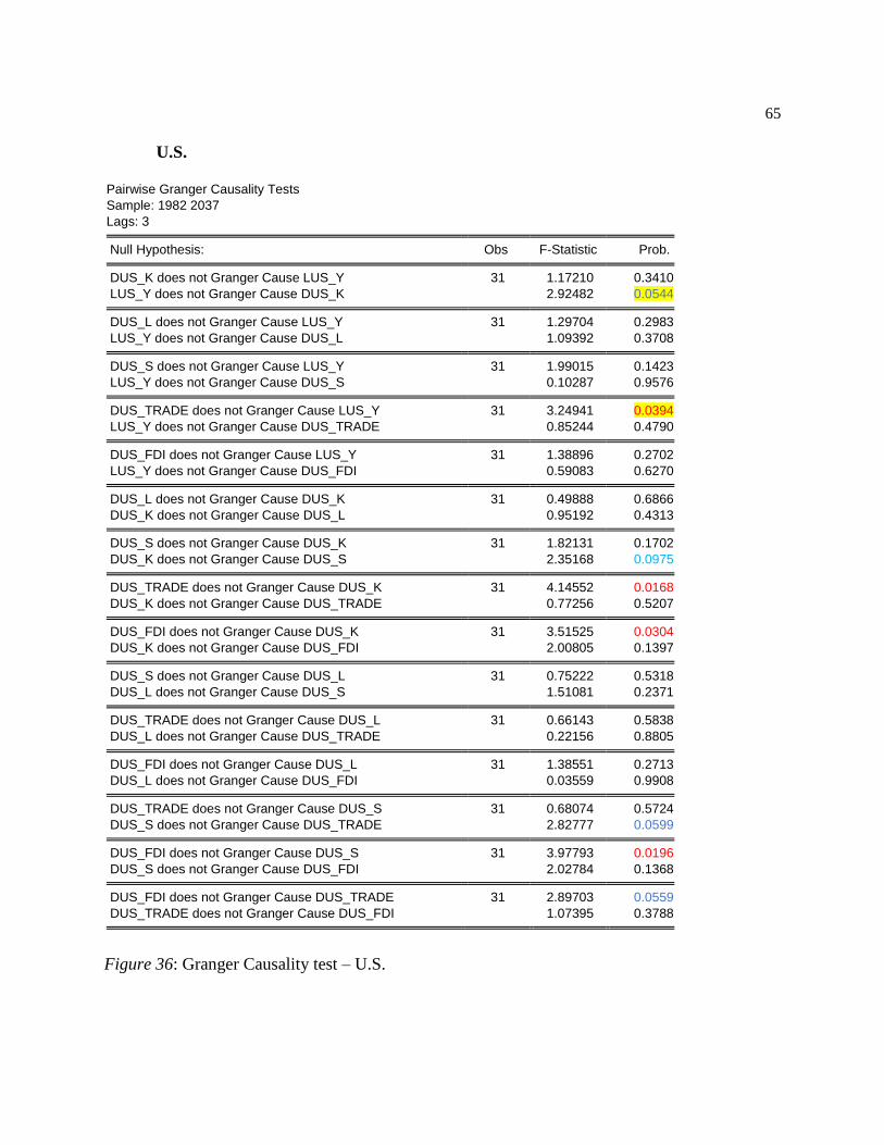
65

U.S.

Pairwise Granger Causality Tests

Sample: 1982 2037

Lags: 3

Null Hypothesis: Obs F-Statistic Prob.

DUS_K does not Granger Cause LUS_Y 31 1.17210 0.3410

LUS_Y does not Granger Cause DUS_K 2.92482 0.0544

DUS_L does not Granger Cause LUS_Y 31 1.29704 0.2983

LUS_Y does not Granger Cause DUS_L 1.09392 0.3708

DUS_S does not Granger Cause LUS_Y 31 1.99015 0.1423

LUS_Y does not Granger Cause DUS_S 0.10287 0.9576

DUS_TRADE does not Granger Cause LUS_Y 31 3.24941 0.0394

LUS_Y does not Granger Cause DUS_TRADE 0.85244 0.4790

DUS_FDI does not Granger Cause LUS_Y 31 1.38896 0.2702

LUS_Y does not Granger Cause DUS_FDI 0.59083 0.6270

DUS_L does not Granger Cause DUS_K 31 0.49888 0.6866

DUS_K does not Granger Cause DUS_L 0.95192 0.4313

DUS_S does not Granger Cause DUS_K 31 1.82131 0.1702

DUS_K does not Granger Cause DUS_S 2.35168 0.0975

DUS_TRADE does not Granger Cause DUS_K 31 4.14552 0.0168

DUS_K does not Granger Cause DUS_TRADE 0.77256 0.5207

DUS_FDI does not Granger Cause DUS_K 31 3.51525 0.0304

DUS_K does not Granger Cause DUS_FDI 2.00805 0.1397

DUS_S does not Granger Cause DUS_L 31 0.75222 0.5318

DUS_L does not Granger Cause DUS_S 1.51081 0.2371

DUS_TRADE does not Granger Cause DUS_L 31 0.66143 0.5838

DUS_L does not Granger Cause DUS_TRADE 0.22156 0.8805

DUS_FDI does not Granger Cause DUS_L 31 1.38551 0.2713

DUS_L does not Granger Cause DUS_FDI 0.03559 0.9908

DUS_TRADE does not Granger Cause DUS_S 31 0.68074 0.5724

DUS_S does not Granger Cause DUS_TRADE 2.82777 0.0599

DUS_FDI does not Granger Cause DUS_S 31 3.97793 0.0196

DUS_S does not Granger Cause DUS_FDI 2.02784 0.1368

DUS_FDI does not Granger Cause DUS_TRADE 31 2.89703 0.0559

DUS_TRADE does not Granger Cause DUS_FDI 1.07395 0.3788

Figure 36: Granger Causality test – U.S.

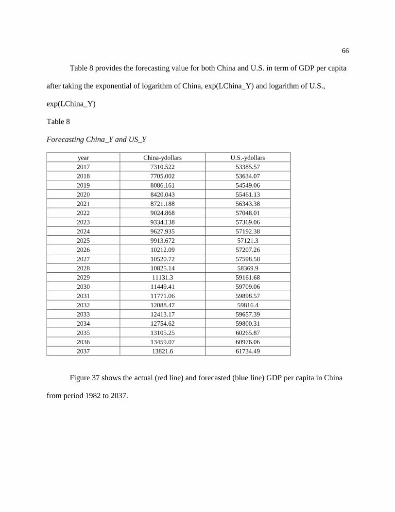
66

Table 8 provides the forecasting value for both China and U.S. in term of GDP per capita

after taking the exponential of logarithm of China, exp(LChina_Y) and logarithm of U.S.,

exp(LChina_Y)

Table 8

Forecasting China_Y and US_Y

year China-ydollars U.S.-ydollars

2017 7310.522 53385.57

2018 7705.002 53634.07

2019 8086.161 54549.06

2020 8420.043 55461.13

2021 8721.188 56343.38

2022 9024.868 57048.01

2023 9334.138 57369.06

2024 9627.935 57192.38

2025 9913.672 57121.3

2026 10212.09 57207.26

2027 10520.72 57598.58

2028 10825.14 58369.9

2029 11131.3 59161.68

2030 11449.41 59709.06

2031 11771.06 59898.57

2032 12088.47 59816.4

2033 12413.17 59657.39

2034 12754.62 59800.31

2035 13105.25 60265.87

2036 13459.07 60976.06

2037 13821.6 61734.49

Figure 37 shows the actual (red line) and forecasted (blue line) GDP per capita in China

from period 1982 to 2037.

67

0

2,000

4,000

6,000

8,000

10,000

12,000

14,000

85 90 95 00 05 10 15 20 25 30 35

NEW_CHINA_Y CHINA_Y

Figure 37: China_Y and Forecasted_China_Y

Figure 38 shows the actual (red line) and forecasted (blue line) GDP per capita in U.S

during the period 1982-2037.

28,000

32,000

36,000

40,000

44,000

48,000

52,000

56,000

60,000

64,000

85 90 95 00 05 10 15 20 25 30 35

NEW_US_Y US_Y

Figure 38: US_Y and Forecasted_US_Y

68

Figure 39: Impulse Response Function – China

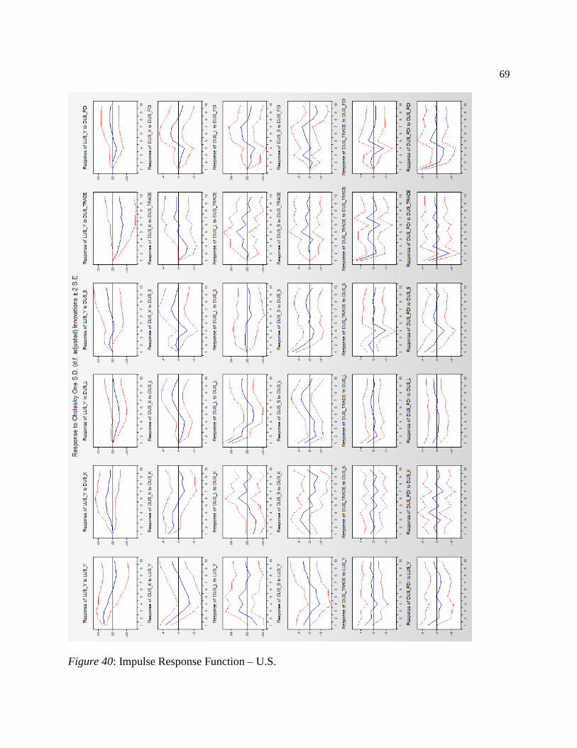
69

Figure 40: Impulse Response Function – U.S.

70

Chapter 5. Conclusion

This paper compares the economic growth in China and U.S. over the period of 1982-

2016 in terms of their GDP per capita and examines whether Chinese economy will surpass the

U.S.’s in the next 20 years, in the period 2017-2037. The OLS regression for China indicates that

at the 5% significant level, capital, and lagged GDP per capita growth are positive and have a

significant effect on GDP per capita growth; saving is also positive and have a significant effect

on GDP per capita growth but at the 10% significant level, which is consistent with the finding

of Misztal (2011) and Krieckhaus (2002) that saving is the determinant of economic growth and

higher saving can cause an increase in economic growth. It is also consistent with the economic

growth theories from Harrod and Domar (1939; 1946), Lewis (1954) and Romer (1986), which

stated the positive relationship between saving and output growth rate. Labor, on the other hand,

is negative and has a significant effect on GDP per capita growth at 5% significant level. The

OLS regression for U.S. indicates that capital, FDI and GDP per capita in last year are positive

and have a significant effect on GDP per capita growth in the U.S.

Even though Table 3 and Table 6 shows the growth of GDP per capita in China as close

to that of the U.S. (8.9-9.5% and 10.9-11.0%, respectively), Figure 37 and Figure 38 tell a

completely different story. They show that by year 2037, GDP per capita in China is slightly less

than $14,000 but GDP per capita in the U.S. is slightly above $61,000, a humongous gap

between the two countries. Table 8 provides the exact value amounts for both China and U.S. in

the period 2017-2037 using VAR forecasting. This finding is not surprising at all. With

approximately 1.4 billion of people, it is extremely hard for China to achieve a high GDP per

capita. If China wants to have the similar amount of GDP per capita as in the U.S. by 2037, then

its GDP need to be approximately 85.4 trillion!

71

This thesis excludes important variables like R&D and government spending on

education due to unavailable data; if possible, for the future research, theses variables can be

included to see whether adding them, more independent variables would become statistically

significant and the effect of the added variables in explaining the impact on economic growth. If

possible, future research should also use labor force participation rate for labor instead of using

population growth rate as a proxy to see if this plays a role in the significance of the variable.

Furthermore, future research can increase sample size to minimize the variance.

72

References

Agrawal, P. (2001). The relation between savings and growth: Cointegration and causality

evidence from asia. Applied Economics, 33(4), 499-513. Retrieved from https://search-

proquest-com.libproxy.stcloudstate.edu/docview/56971300?accountid=14048

Balassa, Bela. 1971. The Structure of Protection in Developing Countries. Baltimore, Md.: Johns

Hopkins University Press.

Bhagwati, Jagdish N., and T N. Shrinivasan. 1978. Trade policy and development. In

International economic policy: Theory and evidence, edited by Rudiger Dornbusch and

Jacob A. Frenkel. Baltimore: The Johns Hopkins Uni- versity Press, pp. 1-38.

Birdsall, Nancy M.; Campos, Jose Edgardo L.; Kim, Chang-Shik; Corden, W. Max; MacDonald,

Lawrence [editor]; Pack, Howard; Page, John; Sabor, Richard; Stiglitz, Joseph E.. 1993.

The East Asian miracle : economic growth and public policy : Main report (English). A

World Bank policy research report. New York, New York : Oxford University Press.

Carroll, C. D. and D. N. Weil, "Saving and Growth: A Reinterpretation", Carnegie- Rochester

Series on Public Policy, 1994, Vol. 40, pp. 133-92

Chen, C. (2011), Foreign Direct Investment in China: Location determinants, investor

differences and economic impacts, Cheltenham, UK: Edward Elgar. doi.org/ 10.4337/

9781781001141.

Chen, C. (2017), Foreign Direct Investment and the Chinese Economy: A critical assessment,

Cheltenham, UK: Edward Elgar. doi.org/10.4337/9781785369735.

Chen, C. (2018). The liberalisation of FDI policies and the impacts of FDI on China’s economic

development. In Garnaut R., Song L., & Fang C. (Eds.), China’s 40 Years of Reform and

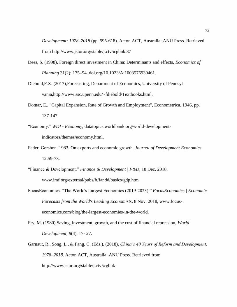
https://search-proquest-com.libproxy.stcloudstate.edu/docview/56971300?accountid=14048

https://search-proquest-com.libproxy.stcloudstate.edu/docview/56971300?accountid=14048

73

Development: 1978–2018 (pp. 595-618). Acton ACT, Australia: ANU Press. Retrieved

from http://www.jstor.org/stable/j.ctv5cgbnk.37

Dees, S. (1998), Foreign direct investment in China: Determinants and effects, Economics of

Planning 31(2): 175–94. doi.org/10.1023/A:1003576930461.

Diebold,F.X. (2017),Forecasting, Department of Economics, University of Pennsyl-

vania,http://www.ssc.upenn.edu/~fdiebold/Textbooks.html.

Domar, E., "Capital Expansion, Rate of Growth and Employment", Econometrica, 1946, pp.

137-147.

“Economy.” WDI - Economy, datatopics.worldbank.org/world-development-

indicators/themes/economy.html.

Feder, Gershon. 1983. On exports and economic growth. Journal of Development Economics

12:59-73.

“Finance & Development.” Finance & Development | F&D, 18 Dec. 2018,

www.imf.org/external/pubs/ft/fandd/basics/gdp.htm.

FocusEconomics. “The World's Largest Economies (2019-2023).” FocusEconomics | Economic

Forecasts from the World's Leading Economists, 8 Nov. 2018, www.focus-

economics.com/blog/the-largest-economies-in-the-world.

Fry, M. (1980) Saving, investment, growth, and the cost of financial repression, World

Development, 8(4), 17- 27.

Garnaut, R., Song, L., & Fang, C. (Eds.). (2018). China’s 40 Years of Reform and Development:

1978–2018. Acton ACT, Australia: ANU Press. Retrieved from

http://www.jstor.org/stable/j.ctv5cgbnk

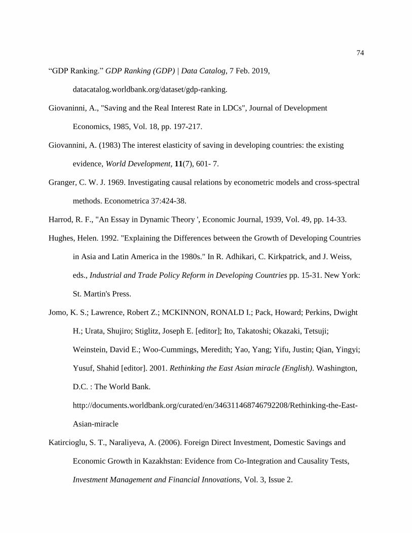
74

“GDP Ranking.” GDP Ranking (GDP) | Data Catalog, 7 Feb. 2019,

datacatalog.worldbank.org/dataset/gdp-ranking.

Giovaninni, A., "Saving and the Real Interest Rate in LDCs", Journal of Development

Economics, 1985, Vol. 18, pp. 197-217.

Giovannini, A. (1983) The interest elasticity of saving in developing countries: the existing

evidence, World Development, 11(7), 601- 7.

Granger, C. W. J. 1969. Investigating causal relations by econometric models and cross-spectral

methods. Econometrica 37:424-38.

Harrod, R. F., "An Essay in Dynamic Theory ', Economic Journal, 1939, Vol. 49, pp. 14-33.

Hughes, Helen. 1992. "Explaining the Differences between the Growth of Developing Countries

in Asia and Latin America in the 1980s." In R. Adhikari, C. Kirkpatrick, and J. Weiss,

eds., Industrial and Trade Policy Reform in Developing Countries pp. 15-31. New York:

St. Martin's Press.

Jomo, K. S.; Lawrence, Robert Z.; MCKINNON, RONALD I.; Pack, Howard; Perkins, Dwight

H.; Urata, Shujiro; Stiglitz, Joseph E. [editor]; Ito, Takatoshi; Okazaki, Tetsuji;

Weinstein, David E.; Woo-Cummings, Meredith; Yao, Yang; Yifu, Justin; Qian, Yingyi;

Yusuf, Shahid [editor]. 2001. Rethinking the East Asian miracle (English). Washington,

D.C. : The World Bank.

http://documents.worldbank.org/curated/en/346311468746792208/Rethinking-the-East-

Asian-miracle

Katircioglu, S. T., Naraliyeva, A. (2006). Foreign Direct Investment, Domestic Savings and

Economic Growth in Kazakhstan: Evidence from Co-Integration and Causality Tests,

Investment Management and Financial Innovations, Vol. 3, Issue 2.

75

Kennedy, Simon. “China Will Overtake the U.S. in Less Than 15 Years, HSBC Says.”

Bloomberg.com, Bloomberg, 25 Sept. 2018, www.bloomberg.com/news/articles/2018-

09-25/hsbc-sees-china-economy-set-to-pass-u-s-as-number-one-by-2030.

Krieckhaus, J. (2002). Reconceptualizing the Developmental State: Public Savings and

Economic Growth, World Development, Vol. 30 Nr 10.

Krueger, Anne O. 1980. Trade policy as an input to development. American Economic Review

70:288-92.

Krueger, Anne. 1993. "American Bilateral Trading Arrangements and East Asian Interests." In

Takatoshi Ito and Anne 0. Krueger, eds., Trade and Protectionism, pp. 25-40. Chicago:

University of Chicago Press.

Lewis, W. A., "Economic Development with Unlimited Supplies of Labour", The Manchester

School of Economic and Social Studies, 1954, Vol. 22, pp. 139-91.

Lopez-Claros, Augusto. “The GlobalCompetitivenessReport 2006–2007.” Weforum.org, 2007,

www3.weforum.org/docs/WEF_GlobalCompetitivenessReport_2006-07.pdf.

Martha Stinson & Christopher Wignall, 2014. "Fathers, Children, and the Intergenerational

Transmission of Employers," Working Papers 18-12, Center for Economic Studies, U.S.

Census Bureau.

Misztal, Piotr (2011): The relationship between savings and economicgrowth in countries with

different level of economic development, e-Finanse: Financial Internet Quarterly, ISSN

1734-039X, University of Information Technology and Management, Rzeszów,Vol. 7,

Iss. 2, pp. 17-29

https://ideas.repec.org/p/cen/wpaper/18-12.html

https://ideas.repec.org/p/cen/wpaper/18-12.html

https://ideas.repec.org/s/cen/wpaper.html

76

Modigliani, F., The Life Cycle Hypothesis of Saving and Inter country Differences in the Saving

Ratio, in W. A. Eltis, M. F. Scott, and J. N. Wolfe, (Eds.) Induction, Growth and Trade:

Essays in honour of Sir Roy Harrod, 1970, Oxford, Clarendon, pp. 197-225

Phillips, P. C. B., and P Perron. 1988. Testing for a unit root in time series regression.

Biometrika 75:335-46

Romer, P M. 1986. Increasing returns and long run growth. Journal of Political Economy

94:1002-37

Rostow, W. W., The Process of Economic Growth, 1960, Oxford University press, Oxford.

Saltz, I. S. (1999). An Examination of the Causal Relationship between Savings and Growth in

the Third World, Journal of Economics and Finance, Nr 23

Shapiro, Gary. “China Will Surpass US to Be World's Largest Economy - It's Time for Us to

Shift Gears.” Fox News, FOX News Network, 23 Aug. 2018,

www.foxnews.com/opinion/china-will-surpass-us-to-be-worlds-largest-economy-its-

time-for-us-to-shift-gears.

Solow, R., "A Contribution to the Theory of Economic Growth", Quarterly Journal of

Economics, 1956, Vol.70, pp. 65-94.

“U.S. and World Population Clock.” Population Clock, 8 Apr. 2019,

www.census.gov/popclock/.

Wei, J. (1994), Chinese Foreign Investment Laws and Policies: Evolution and transformation,

Westport, CT: Quorum Books.

Whalley, J. and Xin, X. (2010), China’s FDI and non-FDI economies and the sustainability of

future high Chinese growth. China Economic Review., 21(1), 123–135.

https://doi.org/10.1016/j.chieco.2009.11.004

77

Wooldridge, J. (2016). Introductory Econometrics: A Modern Approach. 6th ed. Cengaga

Learning.

Zestos, George K., and Xiangnan Tao. “Trade and GDP Growth: Causal Relations in the United

States and Canada.” Southern Economic Journal, vol. 68, no. 4, 2002, pp. 859–874.

JSTOR, www.jstor.org/stable/1061496.

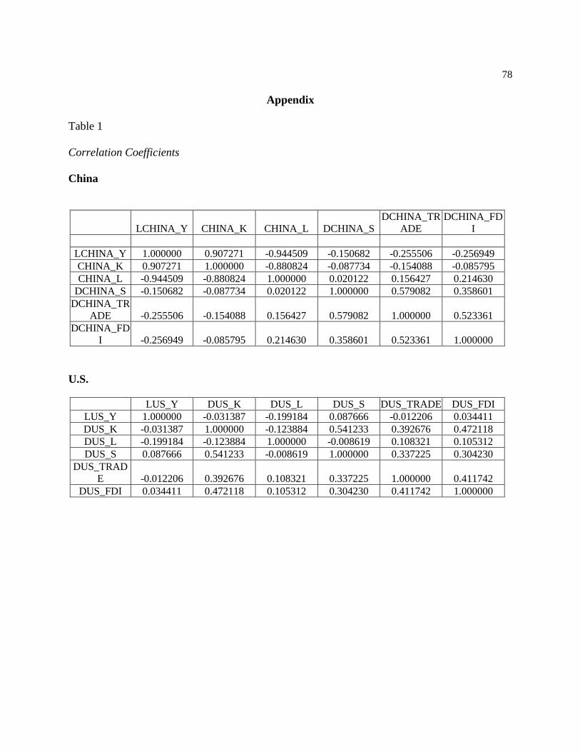
78

Appendix

Table 1

Correlation Coefficients

China


DCHINA_TR

ADE

DCHINA_FD

I

LCHINA_Y 1.000000 0.907271 -0.944509 -0.150682 -0.255506 -0.256949

CHINA_K 0.907271 1.000000 -0.880824 -0.087734 -0.154088 -0.085795

CHINA_L -0.944509 -0.880824 1.000000 0.020122 0.156427 0.214630

DCHINA_S -0.150682 -0.087734 0.020122 1.000000 0.579082 0.358601

DCHINA_TR

ADE -0.255506 -0.154088 0.156427 0.579082 1.000000 0.523361

DCHINA_FD

I -0.256949 -0.085795 0.214630 0.358601 0.523361 1.000000

U.S.


LUS_Y 1.000000 -0.031387 -0.199184 0.087666 -0.012206 0.034411

DUS_K -0.031387 1.000000 -0.123884 0.541233 0.392676 0.472118

DUS_L -0.199184 -0.123884 1.000000 -0.008619 0.108321 0.105312

DUS_S 0.087666 0.541233 -0.008619 1.000000 0.337225 0.304230

DUS_TRAD

E -0.012206 0.392676 0.108321 0.337225 1.000000 0.411742

DUS_FDI 0.034411 0.472118 0.105312 0.304230 0.411742 1.000000

79

Table 2

Descriptive Statistics

China


DCHINA_TR

ADE

DCHINA_FD

I

Mean 7.474667 36.22400 0.919184 0.352306 0.510025 0.039760

Median 7.442907 34.83651 0.826904 0.449499 0.216005 -0.046292

Maximum 8.838474 45.51477 1.610071 3.560879 9.056584 3.573720

Minimum 6.048774 24.56467 0.479150 -2.225028 -12.84744 -1.165728

Std. Dev. 0.852334 6.180659 0.401014 1.612395 4.290952 0.847592

Skewness 0.036053 0.040777 0.370187 0.047490 -0.528534 2.295139

Kurtosis 1.762400 1.904552 1.609415 2.034522 4.258627 10.31646

Jarque-Bera 2.177207 1.709432 3.515998 1.333323 3.827171 105.6850

Probability 0.336686 0.425404 0.172389 0.513420 0.147550 0.000000

Sum 254.1387 1231.616 31.25227 11.97841 17.34085 1.351856

Sum Sq. Dev. 23.97364 1260.618 5.306797 85.79394 607.6050 23.70763

Observations 34 34 34 34 34 34

U.S.


Mean 10.64519 -0.088463 -0.006441 -0.110147 0.266161 0.067117

Median 10.70108 0.098676 -0.019440 0.078608 0.324748 0.063662

Maximum 10.86512 1.071907 0.206610 2.115672 3.416625 1.364265

Minimum 10.28896 -2.467234 -0.123028 -1.991451 -5.175583 -1.789402

Std. Dev. 0.168396 0.709313 0.068515 1.136452 1.557107 0.612352

Skewness -0.435251 -1.143654 1.319254 0.045101 -1.117025 -0.590092

Kurtosis 1.894859 4.859136 5.421198 1.949489 5.978260 4.514412

Jarque-Bera 2.803736 12.30823 18.16722 1.574923 19.63643 5.222226

Probability 0.246137 0.002125 0.000114 0.454998 0.000054 0.073453

Sum 361.9364 -3.007729 -0.219010 -3.745004 9.049472 2.281962

Sum Sq. Dev. 0.935785 16.60311 0.154914 42.62026 80.01118 12.37419

Observations 34 34 34 34 34 34

80

0

10

20

30

40

50

1985 1990 1995 2000 2005 2010 2015

LCHINA_Y CHINA_K

Figure 1: LChina_Y and China_K

-4

-2

0

2

4

6

8

10

12

1985 1990 1995 2000 2005 2010 2015

LUS_Y DUS_K

Figure 2: LUS_Y and DUS_K

81

0

1

2

3

4

5

6

7

8

9

1985 1990 1995 2000 2005 2010 2015

LCHINA_Y CHINA_L

Figure 3: LChina_Y and China_L

-2

0

2

4

6

8

10

12

1985 1990 1995 2000 2005 2010 2015

LUS_Y DUS_L

Figure 4: LUS_Y and DUS_L

82

-4

-2

0

2

4

6

8

10

1985 1990 1995 2000 2005 2010 2015

LCHINA_Y DCHINA_S

Figure 5: LChina_Y and DChina_S

-4

-2

0

2

4

6

8

10

12

1985 1990 1995 2000 2005 2010 2015

LUS_Y DUS_S

Figure 6: LUS_Y and DUS_S

83

-15

-10

-5

0

5

10

1985 1990 1995 2000 2005 2010 2015

LCHINA_Y DCHINA_TRADE

Figure 7: LChina_Y and DChina_Trade

-8

-4

0

4

8

12

1985 1990 1995 2000 2005 2010 2015

LUS_Y DUS_TRADE

Figure 8: LUS_Y and DUS_Trade

84

-2

0

2

4

6

8

10

1985 1990 1995 2000 2005 2010 2015

LCHINA_Y DCHINA_FDI

Figure 9: LChina_Y and DChina_FDI

-2

0

2

4

6

8

10

12

1985 1990 1995 2000 2005 2010 2015

LUS_Y DUS_FDI

Figure 10: LUS_Y and DUS_FDI

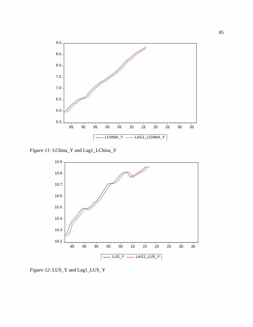
85

5.5

6.0

6.5

7.0

7.5

8.0

8.5

9.0

85 90 95 00 05 10 15 20 25 30 35

LCHINA_Y LAG1_LCHINA_Y

Figure 11: LChina_Y and Lag1_LChina_Y

10.2

10.3

10.4

10.5

10.6

10.7

10.8

10.9

85 90 95 00 05 10 15 20 25 30 35

LUS_Y LAG1_LUS_Y

Figure 12: LUS_Y and Lag1_LUS_Y

Documents

Is China Going to be the World’s Largest Economy