Is Graduate School Worth It? Evaluating the Return on

Union CollegeUnion | Digital Works

Honors Theses Student Work

6-2017

Is Graduate School Worth It? Evaluating theReturn on Investment in a Master's Degree.Kevin Paltat TranUnion College - Schenectady, NY

Follow this and additional works at: https://digitalworks.union.edu/theses

Part of the Econometrics Commons

This Open Access is brought to you for free and open access by the Student Work at Union | Digital Works. It has been accepted for inclusion in HonorsTheses by an authorized administrator of Union | Digital Works. For more information, please contact [email protected].

Recommended CitationTran, Kevin Paltat, "Is Graduate School Worth It? Evaluating the Return on Investment in a Master's Degree." (2017). Honors Theses.95.https://digitalworks.union.edu/theses/95

https://digitalworks.union.edu?utm_source=digitalworks.union.edu%2Ftheses%2F95&utm_medium=PDF&utm_campaign=PDFCoverPages

https://digitalworks.union.edu/theses?utm_source=digitalworks.union.edu%2Ftheses%2F95&utm_medium=PDF&utm_campaign=PDFCoverPages

https://digitalworks.union.edu/studentwork?utm_source=digitalworks.union.edu%2Ftheses%2F95&utm_medium=PDF&utm_campaign=PDFCoverPages

https://digitalworks.union.edu/theses?utm_source=digitalworks.union.edu%2Ftheses%2F95&utm_medium=PDF&utm_campaign=PDFCoverPages

http://network.bepress.com/hgg/discipline/342?utm_source=digitalworks.union.edu%2Ftheses%2F95&utm_medium=PDF&utm_campaign=PDFCoverPages

https://digitalworks.union.edu/theses/95?utm_source=digitalworks.union.edu%2Ftheses%2F95&utm_medium=PDF&utm_campaign=PDFCoverPages

mailto:[email protected]

i

Is Graduate School Worth It? Evaluating the Return on Investment in a Master’s Degree

by

Kevin Paltat Tran

* * * * * * * * *

Submitted in partial fulfillment of the requirements for

Honors in the Department of Economics

UNION COLLEGE June, 2017

ii

Abstract

TRAN, KEVIN PALTAT. Is Graduate School Worth It? Evaluating the Return on Investment in a Master’s Degree. Department of Economics, June 2017

ADVISOR: Eshragh Motahar

Pursuing a college degree is one of the most expensive financial investments that an

individual makes during their lifetime. While several elements contribute to the increasing cost

of obtaining a bachelor’s degree, research indicates that the wage premium of a college degree

remains highly beneficial. Over a lifetime, a bachelor’s degree has an estimated worth of $2.8

million with a wage premium that is 84% greater than individuals holding just a high school

diploma. The tremendous monetary returns and economic opportunities that are associated with a

bachelor’s degree lead to the question as to whether an advanced degree is necessary or worth

the additional financial burden. Master’s degree tuition, opportunity costs of a foregone salary,

and the current $1.4 trillion in outstanding student loan debt, are all factors that must be

considered when evaluating the value of graduate school. While a great deal of research has been

conducted to accurately measure the positive net gains to a bachelor’s degree, less investigation

has been performed for master’s degrees. This study utilizes data from the 2016-2017 PayScale

College Salary Report, the Federal Student Aid Data Center, and U.S. News Higher Education,

to analyze the return on investment of pursuing a master’s degree. The study assesses median

costs and earnings at the school level for master’s degrees in three different academic focuses:

Business, Law, and STEM. Results from the study reveal substantial positive net returns for a

master’s degree at a remarkably high percentage of business and law schools. However, the

financial gains to a master’s degree in STEM concentrations exhibited negative returns compared

to a bachelor’s degree for the majority of the institutions observed.

iii

Acknowledgements

This thesis was supported by the efforts, guidance, and encouragement of Professor Motahar.

Professor Motahar provided extremely useful suggestions and gave critical feedback during the

production of this thesis. His commitment and dedication over the past year have greatly

contributed to the quality of this study. Thank you to Professor Motahar for his continuous

support and making the process of this thesis such a rewarding and valuable experience.

iv

Table of Contents

Chapter One

Introduction………………………………………………………………………………1 A. Current Context………………………………………………………………………...1

Chapter Two

Review of Literature……………………………………………………………………..3 A. Historical Context of College Costs…………………………………………………..3

Section I…………………………………………………………………………...3 Section II…………………………………………………………………………..7

B. Value of Graduate School……………………………………………………………13 C. Review of Findings…………………………………………………………………..18

Chapter Three

Data and Methodology………………………………………………………………....19 A. Evaluating the Data………………………………………………………………….19 B. Methodology……………………………………………………………………….. .25

Section I………………………………………………………………………….25 Section II………………………………………………………………………....26 Section III………………………………………………………………………...28

Chapter Four

Results and Analysis……………………………………………………………………31 A. Calculation Results……...…………………………………………………………...31

Section I………………………………………………………………………….31 Section II………………………………………………………………………....37 Section III………………………………………………………………………...43

Chapter Five

Conclusion………………………………………………………………………………49 A. Summary of Results………………………………………………………………….49 B. Limitations…………………………………………………………………………...50 C. Concluding Remarks………………………………………………………………....52

v

Lists of Tables and Graphs

Tables________________________________________________________________________

Table 3.1: Data Description……………………………………………………………………...23

Table 4.1: Business Net Returns…………………………………………………………………32

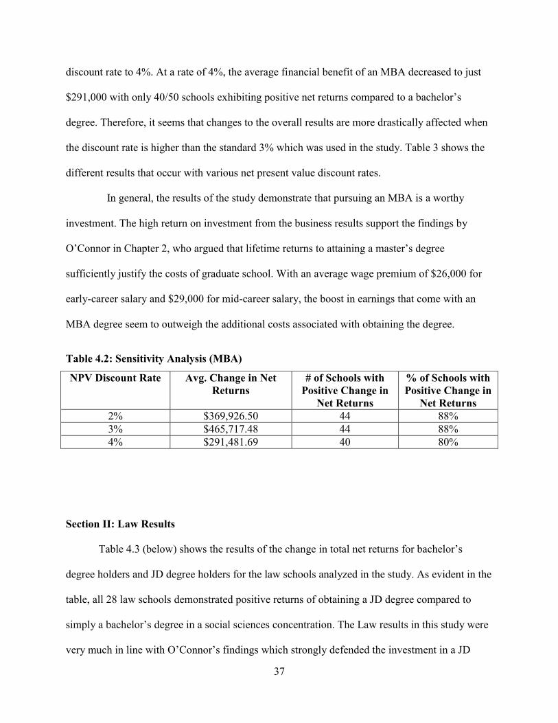
Table 4.2: Sensitivity Analysis (MBA)………………………………………………………….37

Table 4.3: Law Net Returns……………………………………………………………………...38

Table 4.4: Sensitivity Analysis (JD)……………………………………………………………..42

Table 4.5: STEM Net Returns…………………………………………………………………...44

Table 4.6: Sensitivity Analysis (STEM)…………………………………………………………48

Graphs_______________________________________________________________________

Graph 1: Median Mid-Career Salary (MBA)…………………………………………………….34

Graph 2: Difference in Mid-Career Salary (MBA)………………………………………………35

Graph 3: Business School Rank………………………………………………………………….36

Graph 4: Median Mid-Career Salary (JD)……………………………………………………….40

Graph 5: Difference in Mid-Career Salary (JD)…………………………………………………41

Graph 6: Difference in Mid-Career Salary (STEM Master’s)…………………………………...45

Graph 7: Undergraduate School Rank…………………………………………………………...47

Graph 8: STEM Master’s Program Tuition Cost………………………………………………...48

1

Chapter One

Introduction

A. Current Context

This section introduces the research question and outlines the recent trends in college tuition costs and the outstanding student loan debt. This section also discusses the economic relevance of the study for students and the overall economy

The cost of higher education has increased at a staggering rate over the past few decades.

Tuition and fee costs at both private and public universities have surged at a rate significantly

outpacing that of inflation, causing great financial burden on college students and their families.

Measured in 2016 dollars, from the 2006-2007 academic year to the 2016-2017 academic year,

tuition and fees have increased by 68% at private 4-year institutions and an astounding 112% at

public 4-year colleges (CollegeBoard). Rising costs have made college degrees an extremely

expensive investment and have consequently forced a growing number of students to rely on

student loans in order to pursue a college education. Currently, student loan debt in the United

States has exceeded $1.4 trillion and has encumbered recent graduates as evident in high

delinquency and default rates among young Americans. Although trends of mounting tuition

costs and indebtedness continue to persist in the United States, strong evidence still indicates that

the monetary returns to a bachelor’s degree outweigh the increasing costs for the majority of

individuals. If obtaining a bachelor’s degree is such an optimal investment, the question is then

raised as to whether pursuing a master’s degree is worth the additional financial costs.

Obtaining a master’s degree requires several other costs including the tuition and fees for

master’s programs, the opportunity cost of a salary while in school, as well as additional student

loan debt. This thesis will attempt to measure the financial returns to graduate school and

2

determine whether the increased earnings to a master’s degree over an entire work career lead to

a total future net return that is greater than a bachelor’s degree. The study will be broken down

into three academic concentrations: Business, Law, and Science, Technology, and Medicine

(STEM). The study will analyze early career and mid-career earnings data along with various

cost factors for each academic concentration in an effort to identify which variables have the

strongest effects on the net returns to a master’s degree.

The financial well-being of college graduates has implications that affect our economy

and society as a whole. Higher levels of educational attainment often create highly skilled and

efficient workers who are capable of making significant contributions in the workforce. In an

economic perspective, productive workers will thus likely generate the highest salaries and have

the ability to fuel economic growth through consumption. Conversely, if the earnings received

by college graduates do not sufficiently compensate the financial costs and escalating student

loan debt levels required to obtain the degree, economic growth will be stunted due to limited

financial flexibility and disposable income. Even more detrimental, if college graduates fall

behind on their student loan payments, damaged credit scores will further inhibit their ability to

consume major goods and result in a snowball effect of increasing debt and falling consumption

within the country. Therefore, finding from this study have the potential to not only inform

students about the factors that most significantly affect the returns to graduate school, but also

help steer the economy towards a path of economic prosperity with improved financial security

and flexibility for college graduates.

3

Chapter Two

Review of Literature

A. Historical Context of College Costs

Section I will focus on the history of the student loan system and differentiate the four major sources of federal student loans, as well as the contrasting aspects of borrowing as an undergraduate student versus a graduate student. Section II will discuss the main factors which have contributed to the growing outstanding student loan debt and the rise in cost to higher education

Section I: Implementation of Student Loan System

The decision to attend a college or university involves a major financial investment that is

one of the most expensive expenditures that an individual makes during their lifetime. In order to

pursue a degree in higher education, prospective students must be willing to sacrifice a large sum

of money in the present, in terms of both tuition and fee costs along with the opportunity cost of

a salary, in hope that the college degree they earn will lead to significantly higher future

earnings. Realizing that not all high school graduates are financially capable of paying for the

immediate costs to attend college, the U.S. federal government passed the Higher Education Act

in 1965 which introduced the first student loan program that guaranteed repayment to banks and

non-profit lenders (Avery and Turner, 2012). Today, there are currently four major sources of

federal student loans: Stafford Loans (Subsidized), Stafford Loans (Unsubsidized), Parent Loans

for Undergraduate Programs (PLUS), and the Perkins Loans Program. Before I discuss the main

causes that have led to the massive outstanding student loan debt and analyze the benefits of an

advanced degree, I will provide an overview of the different sources of federal aid for higher

education and how each is different from others.

4

The Stafford Loans Program has by far been the largest federal student loan program

dating back to 1965 (Avery and Turner, 2012). At its inception, the program was solely made up

of subsidized loans which were intended to provide aid to eligible undergraduate students who

came from less fortunate backgrounds and who demonstrated a need for financial assistance

(Federal Student Aid). Subsidized Stafford Loans offer advantages over ordinary private market

loans such as a lower rate of interest (currently 3.76%) as well as a temporary deferral of

repayment, meaning that the U.S. Department of Education pays the interest on a student’s loan

while he/she is enrolled up until he/she is 6 months out of college (Avery and Turner, 2012).

According to the Federal Student Loan Data Center, subsidized Stafford loans has risen from

$5.5 billion during the 2005-2006 academic year up to $23 billion for the 2015-2016 academic

year.

Unsubsidized Stafford Loans, on the other hand, were not introduced until 1992 but

provided another source of loans for underprivileged students as well as students who were

ineligible for the Stafford unsubsidized loans (Federal Student Aid). Although Unsubsidized

Stafford Loans may be beneficial for receiving immediate funds, they are less advantageous than

subsidized loans. Students who accept Stafford Unsubsidized Loans are responsible for paying

interest during all periods (including while in school). Therefore if you are unable to pay the

interest while you are in school, the interest will be accumulated and capitalized on the principal

amount of the loan (Federal Student Aid). For that reason, unsubsidized Stafford Loans are much

riskier and can lead to extremely high debt levels if student borrowers are not vigilant about

making regular payments on the loan. Even so, unsubsidized Stafford Loans have still grown

immensely in the United States. From 2006 to 2016, unsubsidized Stafford Loans skyrocketed

from just under $5 billion to over $49 billion (Federal Student Loan).

5

The Direct PLUS loans were established in 1980 for parents of dependent undergraduate

students and graduate/professional level students (Federal Student Aid). Eligibility and loan

amount were determined by one’s historic credit score and the cost of attendance at a given

institution minus all other financial assistance (Federal Student Aid). Direct PLUS loans have

higher interest rates than Stafford Loans at a current rate of about 6.3% (Federal Student Aid).

The exact time in which interest begins to accumulate for Direct PLUS loans varies depending

on whether the borrower is a student or a parent. Students are not charged interest while they are

enrolled in school at-least halftime up to 6 months after leaving, while parents are expected to

begin making payments right when the full amount of their loan is received (Federal Student

Aid). Direct PLUS loans have also seen an uptick in the past decade, growing from $2.2 billion

in the 2005-2006 academic year up to $20 billion in the 2015-2016 academic year (Federal

Student Aid).

Lastly, the Federal Perkins Loan Program (previously called the National Defense

Student Loan Program) provides aid for undergraduate and graduate students with exceptional

financial need (Federal Student Aid). Perkins Loan funds are distributed to colleges and

universities by the federal government with the prior responsible for allocating these loans to

students (Avery and Turner, 2012). Recipients of Perkins Loans are simply charged interest at

5% and are not due to make payments on the loan until 9 months after graduating or leaving

school (Federal Student Aid). Since not all academic institutions participate in the Perkins Loan

Program and aid is only provided to students in extreme situations, the total loan amount is

relatively low compared to other student loan types. During the 2014-2015 academic school

year, the program distributed just over $1 billion to 528,000 students across the country (Federal

Student Aid).

6

Now that the major federal loan programs have been introduced, it is important to

compare the differences between loans at the undergraduate level versus loans at the graduate

school level. Although the 1.4 trillion dollar student loan debt accounts for both groups of

students, it would be a mistake to assume that graduate student loans are the same as

undergraduate loans as they differ in quite significant ways. Generally speaking, undergraduate

borrowers receive more favorable terms on their student loans than graduate borrowers. In terms

of time of repayment, subsidized loans are not even offered to graduate students meaning that the

interest on their loans accrue while they are full time students (Macklin, 2016). Additionally,

interest rates tend to be higher for students at the graduate level. For a graduate student, current

interest rates for a subsidized loan is at 5.31% while PLUS loans demand an interest of 6.3%

(Federal Student Aid). Undergraduates on the other hand, are only charged 3.76% interest for

both direct subsidized and unsubsidized loans. Despite higher interest rates offered to graduate

students, the rates offered by federal government are almost always lower than private lenders.

The industry average interest rate for private lenders ranges from about 9% to 12%, but can soar

up to 18% if the loan offered is variable and based on market conditions (Federal Student Aid).

One arguable advantage that graduate borrowers have over undergraduate borrowers is the limit

to which they are allowed to borrow. Graduate students are permitted to borrow up to $20,500 a

year for direct subsidized loans and are able to aggregate up to $138,500 of loans including the

amount borrowed while completing a bachelor’s degree (Federal Student Aid). Alternatively,

undergraduates are only allowed to borrow up to $31,000 in direct loans during their total 4 years

in school (Federal Student Aid). Higher borrowing limits for postgraduates make pursuing a

graduate degree attainable for a greater number of students, although it does come at a greater

risk for these borrowers. With large outstanding balances and higher interest rates that accrue

7

immediately, graduate students must be cautious of due payments and be very confident that

their increased future earnings with an advanced degree will compensate the total student loan

amount borrowed.

Section II: Factors Contributing to Massive Student Loan Debt Level

The student loan debt total in the United States has skyrocketed in the past decade and

has caused much speculation about whether the debt level is a bubble just waiting to burst.

Americans owe over $1.4 trillion in student loan debt to date, which surpasses outstanding debt

for credit cards and auto loans, and is now the second largest source of household debt only

behind housing mortgages (Dynarski, 2016). Dynarski (2016) explains that of the 40 million

Americans who have accumulated this tremendous debt, 7 million borrowers are in default while

millions more are behind on their payments. The increasing level of student debt has become an

extremely controversial topic both economically and politically. Berman (2016) explains that the

burden of student loan debt has inhibited young Americans in making big purchases such as

houses, cars, and reaching other milestones which enhance their personal lifestyles and

ultimately fuel economic growth. The restraint in financial flexibility that has become the norm

for college graduates brings into questions whether students today are overvaluing a degree at

both the undergraduate and graduate level. A variety of factors can help explain why student debt

has been amassing at its current rate and how it has become an almost universal American

experience. The mountain of debt did not grow overnight. Paul and Wilson (2016) point to the

fact that the total outstanding debt that was just $250 billion a decade ago, has increased more

than fivefold to date. Government policy, profiting off student debt, increase in college

8

enrollment and tuition, and stagnant wage growth, all have contributed to the student loan debt

crisis that exists today.

Although federal aid has remained consistent over the past few decades, the decline of

state aid in the higher education sector has been a prominent cause of rising student loans. With

much opposition for tax increases (especially for the wealthiest Americans) from many powerful

right-wing politicians and supporters, state governments have been unable to generate sufficient

revenue in order to offset the costs for state colleges and universities (Foroohar, 2016). Foroohar

(2016) points out that in many conservative dominant states like Texas, Virginia, and North

Carolina, tax cuts came at a time when state budgets were already being tightened due to events

such as the savings and loan crisis, the dot-com bubble, and the financial crisis of 2007. Before

2008, states provided about $9,000 per student in higher education (Foroohar, 2016). Foroohar

(2016) tells us that today the average state aid per student for higher education has fallen to

$7,000, the lowest it has been in 30 years.

A lack of funds from state governments has resulted in considerably higher sticker prices

at academic institutions. Mitchell (2015) observed that college tuition and fees at both public and

private colleges have risen sharply. From 1995-2015 tuition and fees at private National

Universities has jumped 179%, while in-state tuition and fees at public national universities has

increased by a staggering 296% according to Mitchell (2015). Both increases are significantly

outpacing the rate of inflation, which is evident in the fact that the consumer price index has only

grown by about 55% in the same period (Mitchell, 2015). This means that much of the extra

costs of college are coming straight out of the pockets of students and their families. Foroohar

(2016) explains that the cut in state aid and rising tuition has had the most detrimental effects on

the least financially fortunate Americans due to the wealth divide that has occurred over the

9

same period of time. The average net price of college education as a percentage of family income

has risen moderately for the top 75% of the socioeconomic spectrum, while the price has

skyrocketed for those in the bottom quartile, who paid 44% of their income for a degree in 1990,

versus 84% today. Berman (2016) also demonstrates the diminished impact of the Federal Pell

Grant in 1980 to today in order to exhibit the true effect of tuition growth. She highlights the fact

that this grant which used to cover more than half the costs of a 4-year college now covers less

than a third of the total cost (Berman, 2016). With diminishing financial assistance from state

governments and the cost of colleges rapidly increasing, student loan debt has become inevitable

for the majority of students pursuing a college degree.

Even though college prices have been growing at extraordinary rates, enrollment into

higher education has increased immensely. More and more students are starting to believe that

investing in a college degree today will lead to better financial security in the future, and

statistics seem to support their belief. Avery and Turner (2012) explain that the earnings

premium for a college degree relative to a high school degree has nearly doubled in the past three

decades. Furthermore, the unemployment rate for individuals with a bachelor’s degree is more

than 4% lower than that of individuals with only a high school diploma (Avery and Turner,

2012). Seeing the benefits in a college degree, Dynarski (2014) illustrates that college enrollment

rose about 32% in the decade between 2001 and 2011, which partially helps to explain the

increase in borrowing for student loans. It is worth noting though that not only did the number of

students enrolled in colleges increase, but so did the annual borrowing per student (Dynarski,

2014). Dynarski (2014) shows that from 2001-2011, annual borrowing per student increased

54% from $3,500 to $5,400. Although there clearly are advantages to a college degree, it may be

time to assess where the line must be drawn.

10

Stagnant growth in wages occurring simultaneously with rising college costs is another

important factor in explaining high student loan debt levels. Foroohar (2016) explains that taking

out a small amount of debt to pay for a college education a few decades ago meant simply

getting a summer job, but today’s bachelor degree holders have debt balances averaging $35,000.

This signifies that the proportion of an individual’s and family’s wealth that is put toward higher

education has increased tremendously. Dynarski (2016) though, argues that it is not the amount

of student loans taken out that is the issue, but rather the low earnings that cause young

Americans to default or become delinquent on their loans. Foroohar (2016) sheds light on an

interesting phenomenon, clarifying that although the media often highlights individual cases of

students having $100,000 plus in student loans, it is actually the students with lower loan

balances that have the hardest time repaying their loans. Therefore, the findings from both

Foroohar and Dynarski reveal that default rates are highest among those with the smallest student

debts. Of those borrowing less than $5,000 for college, the default rate is 34%. On the other

hand, the rate of default is just 18% for those borrowing more than $100,000 explains Dynarski

(2016). The explanation for this odd statistic is rooted in the notion that those who take out large

student loan debts often are attending elite institutions or pursuing a graduate degree, two

scenarios that have heavy price tags. Although these students tend to rack up large student loan

debts, they are also building up great human capital which leads to higher salaries, allowing them

to stay on track to pay off their loans (Dynarski, 2016). This is apparent in the fact that only 2%

of graduate students default on their student loans compared to 21% of for-profit

college/community college borrower, says Dynarski (2016). Looney and Yannelis (2015) help to

elucidate that those who borrow lower amounts often are only receiving associate’s degrees at

for-profit or community colleges, where they are not acquiring the necessary credentials or

11

growing their human capital substantially enough to compete for high paying jobs with students

attending more selective 4-year colleges. Looney and Yannelis (2015) found that borrowers at

for-profit and community colleges exiting school in 2010 earned a modest median salary of

about $22,000. In an economy where salaries for middle and low wage workers have been

stagnant for the past three decades, the potential for significant wage growth for individuals with

these degrees are very low. Berman (2016) shows that from 1979-2013, real hourly wages has

increased just 5% for middle wage Americans while real rates for low wage Americans has

actually decreased by 6%. With tuition increases continuing to outpace the growth of wages, it is

no mystery why default and delinquency rates have become a serious issue among student

borrowers.

The alleged profits that are being made by the government and for-profit colleges have

also become a growing concern, especially since it comes at the expense of students’ financial

well-being. The controversy regarding stable returns and profitability in exchange for higher

tuition costs and fees has gained significant uproar. Foroohar (2016) highlights the recent scandal

surrounding Trump University as well as the publicized news that Bill Clinton has received over

$17 million while serving as an honorary chancellor of the for profit college, Laureate

International Universities. Especially during an election year where the student loan debt issue

has been a hot topic, for-profit colleges and increased college costs in general have been under

immense scrutiny. Foroohar (2016) explains that investors view students as “federally subsidized

annuities” through their grants and student loans, which give them great confidence that they will

receive large returns on their investments. The statistics that Foroohar shed light on surely seems

to support these investors’ belief as well. The For-Profit college industry is a $35 billion industry

which saw enrollment grow by nearly 60% in the 1990’s (compared to 7% in the non-profit

12

sector) with a stock price (FPCU) that rose more than 460% from 2000 to 2003

(Foroohar, 2016). However, the success and the growth of for-profit colleges and universities is

not the concern, states Foroohar; rather, the higher price tag and how the profits of these schools

are being allocated. In 2009 thirty leading for-profit colleges and universities spent a modest 17

percent of their budget on instruction, while allocating a whopping 42 percent on marketing to

new students and paying out existing investors. Foroohar (2016) states that Apollo Group, the

parent group of the University of Phoenix (one of the largest for-profit colleges), recently spent

more money on advertising than Apple, one of the world’s richest companies. The miniscule

share of profit that is actually utilized in academic resources for student development has become

very controversial and brings to questions the value of a college degree from a FPCU. An

investigation from 2010 to 2012 found that while students at FPCU represented only 12 percent

of the post-secondary student population, it received a quarter of all federal aid disbursements

and was responsible for 44 percent of all loan defaults (Foroohar, 2016). A large portion of

defaulters were working-class students who either couldn’t afford to graduate or, once they did,

found their degrees were largely useless in the marketplace. Looney and Yannelis (2015) come

to a similar conclusion, condemning the value of for-profit and community colleges. Looney and

Yannelis (2015) show that the bulk of the increase borrowing in the United States is from

students attending for-profit and community colleges, not those attending standard 4-year

colleges. In 2000, with the exception of the University of Phoenix, the top 25 institutions with

the highest collective federal student loan debt consisted of strictly 4-year public or private

colleges; By 2014, 8 of the top 10 and 13 of the top 25 were for-profit institutions

(Looney and Yannelis, 2015). Though they are borrowing more, students attending these

institutions are faring much poorer in the job market as seen by their higher unemployment rate

13

and default rate (Looney and Yannelis, 2015). The inadequate value of for-profit and community

college degrees contribute heavily to the growing debt crisis and are responsible for the majority

of student loan defaults in the United States.

B. Value of Graduate School

This section will provide statistics and analysis on the wage premium with a master’s degree over a bachelor’s degree. Additionally, this section will identify the specific traits that are enhanced with an advanced degree that make students with graduate degrees more appealing in the workforce

Historic research and analysis from numerous sources have come to the same conclusion

that attaining a bachelor’s degree is pivotal to economic opportunity, and thus earning higher

future earnings. Carnevale (2009) found that the college premium since 1999 has grown

tremendously. Over a lifetime, individuals with a bachelor’s degree earn 84% more than those

with only a high school diploma (Carnevale, 2009). This equates to a bachelor’s degree holding a

worth of about $2.8 million on average. With a 4-year degree already generating significant

advantages over a high school diploma, debate occurs as to whether pursing an advanced degree

is necessary or even worth it. In order to assess the value of obtaining a post-baccalaureate

degree, potential future earnings and additional student loan debt must both be taken into

consideration.

Torpey and Terrell (2015) explain that the payoff to graduate school varies significantly

by industry and occupation, but on average there does exist a substantial wage premium for

individuals with a post-baccalaureate degree. In 2013, the median annual wage for full-time

workers over the age of 25 with a master’s degree was $68,000, a $12,000 a year wage premium

compared to those with only a bachelor’s degree (Torpey and Terrell, 2015). Carnevale (2015)

14

also analyzed the median salaries of individuals with an advanced degree, finding that those with

a master’s degree will make $400,000 more over their lifetime compared to bachelor’s degree

holders and about $1.4 million more than those with just a high school diploma. Despite an

ample median salary increase for those opting to attend graduate school, Torpey and Terell

(2015) reiterate the fact that not all workers earn premiums. A master’s degree varies in value

depending on the desired field that an individual enters; in some cases workers with a master’s

degree earn about the same or even less than those holding a bachelor’s degree (Torpey and

Terrell, 2015). Carnevale’s (2015) research also suggests that an advanced degree does not

always result in higher future earnings, demonstrating that there exists considerable overlap at all

education levels. For example, 17% of people with a bachelor’s degree earn more than the

median salary of those with a professional degree (Carnevale, 2015). Torpey and Terrell (2015)

explain that some occupations such as nurses, economists, and physician assistants, require

advanced degrees just for entry-level positions, although the need for a higher degree within

other occupations is more dubious. Using information from the Bureau of Labor Statistics,

Torpey and Terrell (2015) found that occupations within the field of Business exhibited the

highest returns when comparing the median salaries between individuals with master’s degrees

and bachelor’s degrees. Wage premiums were found to be particularly high for those working in

commodities, sales, and other financial services occupations. The wage premium for workers in

these occupations with a master’s degree was 89% higher than workers with just a 4-year degree

(Torpey and Terrell, 2015). It is no surprise that from 2012-2013, no other field awarded more

master’s degrees than that of business (Torpey and Terrell, 2015). Data from the Bureau of

Labor Statistics also found significant wage premiums due to a master’s degree in the fields of

15

Education, Healthcare Services, and STEM, with wage premiums averaging between 25% and

40%.

Lindley and Machin’s (2013) work help to identify the central skills that are enhanced

with an advanced degree, that make master’s degree holders more appealing to employers

compared to those who opted not to attend graduate school. Lindley and Machin (2013) found

that cognitive, computer, and people skills, were the qualities which were most improved when

attending graduate school. More specifically, individuals with a master’s degree were stronger in

presentations/speeches, mathematics/statistics, and more efficient in using computers (Lindley

and Machin, 2013).

Lindley and Machin (2013) point to technological advancements and a growing reliance

on computers in several industries as a major factor which has boosted the value of attaining an

advanced degree. They explain that the relative demand shifts in favor of workers with

postgraduate qualifications are strongly correlated with technical changes as measured by

computer usage and investment. Valleta (2015) adds that evolving workplace technologies have

undermined the demand for routine jobs, as computer-intensive capital equipment and processes

have readily substituted operational tasks that were previously done by workers. Using Valleta’s

(2015) theory on evolving technologies effect on workers demand in combination with Lindley

and Machin’s (2013) finding that computational skills are strengthened with a master’s degree,

the desire to hire individuals who have attended graduate school becomes more apparent.

Research shows that students who attended graduate school are simply more efficient

complements to computers than those with only a bachelor’s degree. Lindley and Machin (2013)

explain that this has been an important driver of the rising wage premiums, as the presence and

skills held by postgraduates in the workplace has grown in importance. They go on to clarify that

16

postgraduate workers and college only workers are different in the sense that they are not perfect

substitutes for one another; they tend to work in different occupations, with postgraduates filling

the jobs positions that require more advanced skills and a better grasp of computational methods.

It is evident that there exists significant wage premiums (for several occupations at least)

for students who pursue a master’s degree, but in order to assess the true value of the degree,

costs and indebtedness associated with extra schooling must be taken into consideration.

According to Delisle (2014) the median cumulative debt for graduate students in 2012 was

$57,600 (which includes any debt from an undergraduate degree). Depending on the program

that an individual enters though, has a significant impact on the level of indebtedness they will

enter upon graduation. For example, in 2012 the median cumulative debt for a student pursing an

MBA was $42,000, while the median cumulative debt for students graduating with a JD degree

in law was $140,116 (Delisle, 2014). Although a law degree typically require 3-years of

schooling compared to 2-year programs for MBA’s, the debt levels still differ by a considerable

amount. Other aspects that must be considered when evaluating the costs to graduate school

include the actual institution which an individual attends, as well as the opportunity cost of a

foregone salary while remaining in school. According to data from Bloomberg BusinessWeek,

the average total tuition in 2011-2012 for the top 20 business schools in the country was

$102,355, while the average starting salary for the Class of 2012 graduates (from undergraduate

institutions) was $44,442 (O’Connor, 2012). This means that the total cost of attending an elite

business school is close to $200,000, and will likely be higher due to interest rates on any

borrowed funds. The cost of law school typically is even higher. Average tuition costs at the top

law schools in 2011-2012 were about $50,000 per year, meaning that the total tuition cost was

around $150,000 due to the 3-year structure of law programs (O’Connor, 2012). When taking

17

opportunity costs into consideration, law students are investing close to $300,000 for a J.D.

degree with the possibility that the cost is even higher if loan interest is taken into account.

Despite the expensive financial investment required to attend a top graduate program, O’Connor

(2012) argues that lifetime returns to attaining an advanced degree in law or business sufficiently

justify the high price tag of each. Individuals who hold an MBA will earn between $5 million

and $8 million during a 40 year career (O’Connor, 2012). Therefore, those with an MBA only

spend about 3% to 5% of their lifetime earnings on the total cost of attending business school,

including the opportunity cost of a foregone salary. According to a study by the Georgetown

University Center on Education and Workforce, business school graduates earn the same amount

or more working 20 years, than those with just a bachelor’s degree working for 40 years

(O’Connor, 2012). For lawyers, the benefits of the advanced degree appear to outweigh the costs

as well. The Georgetown Study found that lawyers on average will make a little over $4 million

during their career, double the average earnings of an individual with only a bachelor’s degree

(O’Connor, 2012). The data clearly indicates that the full costs of business and law school are

less significant when comparing it to the increased lifetime earnings that result from attending

these institutions. In general, when analyzing the lifetime wage premium against the tuition costs

and debt levels for business and law school, the decision to pursue these degrees are worthwhile

investments.

18

C. Review of Findings

This section will summarize the main ideas and conclusion drawn from current literature and preview the methodology which will be utilized to answer the research question for this study

The outstanding student debt amount along with default rates have increased

exponentially over the past few decades due to several factors such as rising tuition and

enrollment, declining state aid in higher education, stagnant wage growth, and the insufficient

return on investment at for-profit and community colleges. After reviewing characteristics of the

student loan system, it is also important to note that there exist key differences when borrowing

at the undergraduate and graduate level. Graduate borrowers do not receive subsidized loans,

tend to have higher interest rates, and are given higher limits on their borrowing amounts.

Despite the fact that graduate students often have exceptionally high debt levels, they are among

the groups of student who are least likely to default due to a high degree of advanced human

capital which they build in the process. Rather, students attending for-profit and community

colleges as well as other non-selective school are the most likely to struggle paying back their

student loans. When examining the wage premium for individuals with a master’s degree, it

appears that the return on investment is worth the high costs that come with additional schooling

for the majority of students, but not for all fields.

In the next chapter, I will introduce the methodology which will be used to evaluate the

true return on investment of obtaining a master’s degree. The method will essentially involve

several case studies in which I compare median earnings at a school level for bachelor’s degrees

and master’s degree students for different academic concentrations. I will then incorporate

average tuition, opportunity cost, and indebtedness for specific graduate programs in order to

analyze the value of a master’s degree at various institutions.

19

Chapter 3

Data and Methodology

A. Evaluating the Data

This section will provide relevant information on the data sources which will be used for this study; highlighting strengths and potential concerns of each source

This study will use data from four main sources: 2016-2017 PayScale College Salary

Report, Federal Student Aid Data Center, U.S. News Higher Education, and Forbes: America’s

Top Colleges. Initially, the study was intended to analyze earnings and student loan information

at an individual level in order to run and interpret regressions. However, due to a lack of readily

available data and confidentiality concerns, the study will instead examine return on investment

at the school level using a case study methodology. Certain limitations and assumptions occur

when data is evaluated using median and average measures rather than specific individual cases;

however these concerns and the strategic presumptions made will be thoroughly explained

throughout this section.

The 2016-2017 PayScale College Salary Report provides college rankings for over 1,000

schools by salary potential. All data in the report was collected by employees who successfully

completed PayScale’s employee survey, and later was rigorously tested and verified for

accuracy. A useful feature of the PayScale report is the ability to display rankings for different

degree types as well as academic majors. Therefore, users are able to compare median earnings,

both early career pay and mid-career pay, between bachelor’s degree holders and master’s degree

holders from the same institution within the same academic concentration. For example,

PayScale allows users to view the median earnings for individuals who graduate from Boston

20

University with a B.A. in business as well as the median earnings for individuals who received

an MBA from Boston University. Bachelor’s degree is defined as only employees who possess a

bachelor’s degree and no higher degree. Similarly, master’s degree is defined as only employees

who possess a master’s degree and no higher degree. This assures that there is no overlap in the

samples and also helps to avoid an overestimation for bachelor’s degree earnings.

Acknowledging the fact that data is being interpreted at a school level rather than an

individual level, there are certain assumptions and concerns that must be addressed. Only schools

which PayScale had statistically significant samples were considered in the report. Consequently,

there are likely universities that are not present in the report but actually have higher returns on

investment than some schools which were included. Exclusion from the report therefore is not

always a reflection of the quality and value of an institution; rather it is an indication that there

was an insufficient amount of verified data from the school to publish a salary ranking for it. For

example, PayScale was only able to provide median earnings data for 37 law schools, of which

only 28 had corresponding undergraduate programs for comparison. Of the schools included in

the overall report, the average sample size was 325, with much variation due to differences in

school size. Analyzing earnings at the university level between different degree types also makes

the assumption that all individuals who pursue a master’s degree attend the same university

which they received their bachelor’s degree from. There is no feasible way to account for

students who attend a different institution in pursuit of a master’s degree, which is not a rare

path. For instance, it would not be uncommon for an individual to receive a bachelor’s degree

from Boston University, but then pursue an advanced degree at a different institution, such as

UMass Amherst. However, because the study focuses on median earnings, this phenomenon

should not pose as a serious concern.

21

The Federal Student Aid Data Center offers a centralized source for information relating

to the federal financial assistance programs. Since this study will examine earnings and costs

(such as student loans) at the school level, the Federal Student Aida Data Center was extremely

convenient because it provides loan information by academic institution. The Data Center

contains recipient and volume data by loan type for each of the approximately 6,000 schools

participating in the Title IV programs. Student loan data is broken down into 5 direct loan

programs for each school: Subsidized, Unsubsidized – Undergraduate, Unsubsidized – Graduate,

Parent PLUS, and Graduate PLUS. Due to the fact that this study evaluates the return on

investment for the average student at any given university, Parent PLUS and Graduate PLUS

loans will be omitted from the study when calculating the average federal student loan that a

borrower receives. Mentioned previously in Chapter 2, Parent PLUS and Graduate PLUS loans

are only awarded to students and families who demonstrate exceptional financial need. Thus,

these two loan programs do not precisely represent the financial need of the average student

borrower. The exclusion was justified when further examination of the student loan data verified

that only a very small portion of students from each school actually receive these loan types. As

a result, only subsidized direct loans and unsubsidized direct loans (for both undergraduate and

graduate students) were used to estimate average loan amounts in the study. Average loan

amounts were calculated for each school simply by dividing the total dollar amount of loan

disbursed by the number of recipients for each loan program.

Data from U.S. News Higher Education was used to find tuition and fee costs for

undergraduate attendance, as well as specific graduate programs. U.S. News proved to be more

advantageous than other college information sources because the site distinguished the costs for

different degree programs such as MBA and JD degrees. A flaw in the data from U.S. News is

22

that there are no statistics provided on average scholarship and grant awards. Thus, there is no

way to estimate the average net price of attendance at any given institution. Other data sources

such as the National Center for Educational Statistics offered figures for average net costs, but

only at the undergraduate level. Using these other sources consequently would cause

inconsistencies in the analysis since scholarships would only be recognized for undergraduate

schools and not graduate school. Since data for scholarships and grants were unavailable for all

degree types, they will not be considered in the study. Overlooking grants and scholarships could

potentially cause the estimated costs of both undergraduate and graduate school tuition to be

slightly overestimated. Another conjecture that was made using tuition data from U.S. News was

that in-state tuition and fee prices would be used for public universities. In-State tuition and fees

can range to be $10,000-$30,000 cheaper than out-of-state tuition, though the majority of

students at public universities tend to be residents of the state which the school resides in.

Nonetheless, average tuition costs at public universities will be somewhat underestimated due to

the use of in-state tuition. Although some students may be paying the higher out-of-state price

tag, the majority are paying for the cheaper in-state tuition cost making the assumption more

representative of the average student.

U.S. News Higher Education also provided data on graduate rankings program for each

of the three academic concentrations. U.S. News takes several factors into consideration for the

methodology of their rankings including quality assessment by college deans and recruiters,

post-graduation success (employment rate and earnings), as well as mean grade point averages

and test scores. The undergraduate rankings from this source were unusable because rankings for

liberal arts colleges, regional universities, and national universities, are separated into different

groups. Thus, there was no way to feasibly compare schools from the different classification

23

groups. Therefore, data from Forbes: America’s Top Colleges was used because of the

consolidation of all school types into a single rankings list. The methodology for ranking from

Forbes was solely based on the return on investment of a bachelor’s degree from a given

institution.

Data from these sources will be utilized and manipulated to generate the components

which make up total future earnings over a work career as well as the total cost of pursuing a

bachelor’s degree and a master’s degree. Table 3.1 below, displays a detailed description of the

factors that will be considered in the study and exactly how each will be calculated.

Table 3.1: Data Description Field Name Definition School The school name of an academic institution which consists of

both an undergraduate and graduate program Undergrad Rank Forbes rankings of the undergraduate institution based on the

return on investment (Rankings closer to 1 indicate better investment)

Business Rank U.S. News ranking of MBA programs Law Rank U.S News ranking of JD programs STEM Rank U.S. News rankings of master’s degree in engineering Early Career Pay (B.A.) Median salary for alumni with a bachelor’s degree from a specific

school with 0-5 years of work experience Mid-Career Pay (B.A) Median salary for alumni with a bachelor’s degree from a specific

school with 10+ years of work experience Early Career Pay (Master’s) Median salary for alumni with a master’s degree from a specific

school with 0-5 years of work experience Mid-Career Pay (Master’s) Median salary for alumni with a master’s degree from a specific

school with 10+ years of work experience Recipients The number of loan recipients for the loan type during the 2015-

2016 award year. For Subsidized, Unsubsidized, and Graduate PLUS loans, this is a count of student borrowers. For Parent PLUS loans, this is a count of the students on whose behalf the loan was taken.

$ of Loan Disbursed The dollar amount of the loans initiated for the loan type during the 2015-2016 award year. This is the expected total loan amount if the loan is fully disbursed.

24

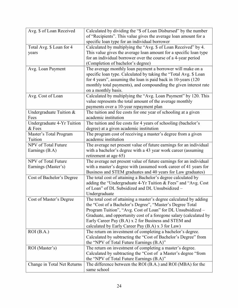
Avg. $ of Loan Received Calculated by dividing the “$ of Loan Disbursed” by the number of “Recipients”. This value gives the average loan amount for a specific loan type for an individual borrower

Total Avg. $ Loan for 4 years

Calculated by multiplying the “Avg. $ of Loan Received” by 4. This value gives the average loan amount for a specific loan type for an individual borrower over the course of a 4-year period (Completion of bachelor’s degree)

Avg. Loan Payment The average monthly loan payment a borrower will make on a specific loan type. Calculated by taking the “Total Avg. $ Loan for 4 years”, assuming the loan is paid back in 10-years (120 monthly total payments), and compounding the given interest rate on a monthly basis.

Avg. Cost of Loan Calculated by multiplying the “Avg. Loan Payment” by 120. This value represents the total amount of the average monthly payments over a 10-year repayment plan

Undergraduate Tuition & Fees

The tuition and fee costs for one year of schooling at a given academic institution

Undergraduate 4-Yr Tuition & Fees

The tuition and fee costs for 4 years of schooling (bachelor’s degree) at a given academic institution

Master’s Total Program Tuition

The program cost of receiving a master’s degree from a given academic institution

NPV of Total Future Earnings (B.A)

The average net present value of future earnings for an individual with a bachelor’s degree with a 43 year work career (assuming retirement at age 65)

NPV of Total Future Earnings (Master’s)

The average net present value of future earnings for an individual with a master’s degree with (assumed work career of 41 years for Business and STEM graduates and 40 years for Law graduates)

Cost of Bachelor’s Degree The total cost of attaining a Bachelor’s degree calculated by adding the “Undergraduate 4-Yr Tuition & Fees” and “Avg. Cost of Loan” of DL Subsidized and DL Unsubsidized – Undergraduate

Cost of Master’s Degree The total cost of attaining a master’s degree calculated by adding the “Cost of a Bachelor’s Degree”, “Master’s Degree Total Program Tuition”, “Avg. Cost of Loan” for DL Unsubsidized – Graduate, and opportunity cost of a foregone salary (calculated by Early Career Pay (B.A) x 2 for Business and STEM and calculated by Early Career Pay (B.A) x 3 for Law)

ROI (B.A.) The return on investment of completing a bachelor’s degree. Calculated by subtracting the “Cost of Bachelor’s Degree” from the “NPV of Total Future Earnings (B.A)”

ROI (Master’s) The return on investment of completing a master’s degree. Calculated by subtracting the “Cost of a Master’s degree “from the “NPV of Total Future Earnings (B.A)”

Change in Total Net Returns The difference between the ROI (B.A.) and ROI (MBA) for the same school

25

B. Methodology

This section will explain how the return on investment will be calculated when receiving a bachelor’s degree and master’s degree. Furthermore, it will provide in depth detail about the costs and benefits considered and how the value of each degree type will be compared.

This case-study is broken into three sections for different academic concentrations:

Business, Law, and Science, Technology, Engineering, and Mathematics (STEM). The sample

size for each academic concentration varies due to the available earnings data for the different

degree types. In order to identify which graduate schools are worth the investment, the study will

compare the return on investment of attaining a bachelor’s degree in one of the three academic

concentrations at a specific university with the return on investment of a master’s degree in the

same academic focus.

Section I: School Sample Selection

For business school observations, the study uses the PayScale 2016-2017 College Salary

Report filtered by “Best Schools for Business Majors by Salary Potential.” This filter sorts all 4-

year schools, for which sufficient earnings data is available, by mid-career pay. Mid-career pay

is defined as median salary for alumni with 10+ years of work experience. The top 50 schools for

mid-career pay of business majors are used in this study and compared to the earnings of Masters

of Business Administration degrees at each respective school.

A different approach was taken while selecting institutions to analyze for law degrees

because of the limited data available on the PayScale report. Earnings are only reported for 37

graduate law schools, while just 28 of those schools actually are affiliated with an undergraduate

26

university which analysis can be performed. Thus, observations for law schools are limited to the

28 universities which earnings data is readily accessible.

Collecting a sample size for STEM schools proved to be slightly more difficult because

there is not a specific degree type, such as an MBA or JD, which all STEM students pursue while

in graduate school. For example, a bachelor’s degree holder in mechanical engineering and a

bachelor’s degree holder in computer science are likely going to pursue different master’s

degrees. Since data is not explicit for STEM degrees, schools were selected simply based on the

percentage of degrees awarded in science, technology, engineering, and mathematics. Only

school which awarded 50% or more of their degrees in STEM, and had a graduate school were

included in the study. This categorization allowed analysis to be performed for 18 schools.

Section II: Calculating Benefits

In order to properly compare the returns to a bachelor’s degree and a master’s degree, it

is pivotal to identify each component that makes up the monetary benefits of each degree. The

only factors that contribute to financial benefits in this study are early career pay and mid-career

pay. The study calculates the net present value of total future earning at each institution using a

discount rate of 3% per year. The rate of 3% was chosen because that is about the average rate of

return than an individual would be able to make through an investment on a financial asset today.

Sensitivity analysis will also be used though, in order to examine whether any major changes to

return on investment occur when the discount rate is slightly modified. The net present value of

nominal future earnings for a bachelor’s degree holder is calculated for 43 years, assuming that

the average worker enters the labor force at age 22 (immediately after graduation) and retires at

27

age 65. Early career pay is the salary amount estimated for the first five years of work, while

mid-career pay is used for the remaining 38 years of a work career.

When computing the net present value of future earnings for a master’s degree holder,

earnings and career length both must be adjusted. The career length for master’s degree holders

is estimated at 41 years for Business and STEM students, and 40 years for law students. The

disparity is due to the fact that Master’s degrees in Business and STEM typically take 2-years to

complete, while a JD degree regularly takes 3 years. For all academic focuses, it is also assumed

that students are pursuing graduate degrees immediately after completion of a bachelor’s degree

and that they are full-time students. It is worth noting that this assumption can have drastic

influence on whether the wage premium of a master’s degree is worth the cost. Entering graduate

school immediately after completing a bachelor’s degree versus after working for several years

can cause considerable differences in the costs and benefits of obtaining a master’s degree.

Individuals who have work experience under their belt often have an advantage over recent

graduates for a few reasons. For one, more experience tends to help applicants get into more

prestigious institutions which are often linked to higher future earnings. Since individuals with

work experience have also likely built up a savings, lower student loan amounts will be needed

for attendance which will decrease the costs to receiving a master’s degree. Lastly, many

employers will actually encourage their associates to pursue an advanced degree by partially

subsidizing the cost of graduate school or in some cases, covering the entire expense. Obviously

these three factors would augment the return on investment for individuals with work experience

by decreasing the total costs of attendance. In this study, the presumption is that graduates with a

Business or STEM degree will enter the workforce at age 24 and retire at 65 while students with

a Law degree will begin working at age 25 and retire at 65. For all academic concentrations,

28

early career pay of specific master’s degrees held will be used for the first 5 years of earnings.

Mid-career earnings for a master’s degree will be used as the salary for the remaining years an

individual has in the work force. The discount rate for future earnings for a master’s degree

holder will also be set at 3%.

Section III: Calculating Costs

Calculating the costs of attaining a bachelor’s degree and master’s degree involves

several factors that must be taken into consideration to determine the total cost. The

“Undergraduate 4-Yr Tuition & Fees” cost which is calculated by multiplying the annual tuition

from U.S. News Higher Education by four, gives the direct cost of attending an undergraduate

institution. Although borrowed student loans and the accumulation of interest on these loans

must also be included in the costs. Average annual subsidized and unsubsidized direct loans were

also multiplied by four to find the average amount borrowed per loan type over the duration of

completing a bachelor’s degree. Then using the PMT function in Excel, average monthly

payments on these two loans can be calculated using a constant interest rate. The study uses an

interest rate of 3.76%, the federal rate as of July 1st 2016, for both unsubsidized and subsidized

undergraduate loans. It is also presumed that the loan term follows the typical 10-year repayment

plan with regular monthly payments. To be able to compute the total average cost of the loan

amount with accrued interest, average monthly payments on both loan types will be multiplied

by 120, the total monthly payments made during the 10 year period. The total average cost of a

subsidized loan in combination with the total average cost of an unsubsidized loan will then be

added to the to the undergraduate 4-yr tuition and fees cost to generate the total cost of a

bachelor’s degree.

29

When estimating the cost of obtaining a master’s degree, the total cost of a bachelor’s

degree will be the first variable incorporated. This being because a bachelor’s degree is a

prerequisite in order to pursue any advanced degree. In addition to the cost of a bachelor’s

degree, master’s degree tuition, graduate student loans, and opportunity cost, will all factor in to

calculate the overall cost of a master’s degree. In terms of finding the total cost of tuition for a

master’s degree program, annual tuition costs will be utilized from the U.S. News Higher

Education website. Annual tuition costs will then be multiplied by two for Business and STEM

degrees and by three for Law degrees, to cover the entire duration of each graduate program.

Direct unsubsidized loans will be the only graduate loan type included and is calculated similarly

to the undergraduate loans. The only difference will be the interest rate which will be adjusted to

5.31%, the current federal rate for unsubsidized graduate loans. Lastly, the opportunity cost of a

salary foregone must be incorporated. Early career earnings from the PaysScale Report will be

multiplied by two for Business and STEM programs and three for Law programs to approximate

the opportunity cost of obtaining these graduate degrees. Adding the total cost of a bachelor’s

degree, tuition for graduate school, the cost of a graduate loan, and the opportunity cost of a

salary, will yield the total cost of a master’s degree for each program at any given school.

Now that the methodology that will be used in determining the financial benefits of a

bachelor’s degree and master’s degree (both through Net Present Value) as well as the total costs

of both degrees have been addressed, the approach the study will use to assess the value of a

master’s degree can now be introduced. Before comparing the benefits of a master’s degree to a

bachelor’s degree, the true value of each degree must be found. The true value for both degrees

will be examined by subtracting the total costs of attaining each degree from the total net present

value of future earnings for an individual holding that same degree. The monetary return on

30

investment will then be known for a bachelor’s degree and master’s degree in the same academic

concentration for each university in the study. Subtracting the monetary return on investment

from a bachelor’s degree holder from a master’s degree holder will thus demonstrate whether

pursuing a master’s degree is financially worth it. If the result is positive, this would indicate a

positive net return to achieving a master’s degree, while a negative result would indicate a

negative net return and that investing in a master’s degree would not be financially

advantageous. After calculating the return on investment for each school included in the study,

deeper analysis will be performed to identify trends and variable correlations to determine

exactly why obtaining a master’s degree at a certain institution may be more advantageous than

others.

31

Chapter Four

Results and Analysis

A. Calculation Results

This section will discuss the general results of the calculated return on investment for all three academic concentrations: Bustiness, Law, and STEM. It will also compare the total net return for each academic focus for bachelor’s degree and master’s degree holder

Section I: Business Results

Table 4.1 (below) displays the Total Net Returns for a B.A., Total Net Returns for an

MBA, and the change between the two degrees, for the academic institutions used in this study.

The results indicate that of the 50 school included, 44 of them or 88% demonstrated that the

financial investment of attaining a master’s degree is worth the cost. The average benefit over a

work career of pursuing an MBA as opposed to holding a bachelor’s degree in business is just

under $370,000. The greatest return for an MBA came from Northwestern University with a Net

Return of $1,218,817 greater than a bachelor’s degree. The school which displayed the poorest

value to obtaining an MBA was Loyola University in Maryland, whose average MBA holder

makes a net return that is $114,682 less than a bachelor’s degree holder.

32

Table 4.1: Business Net Returns

School Name Total Future Net Return (B.A)

Total Future Net Return (MBA)

Change in Total Future Net Return

American University $1,975,490.82 $2,239,763.72 $264,272.90 Babson College $2,403,959.46 $2,781,139.19 $377,179.73 Baylor University $1,878,773.96 $2,249,046.36 $370,272.40 Boston College $2,364,061.51 $2,448,613.61 $84,552.09 Boston University $2,001,945.40 $2,469,633.18 $467,687.77 Brigham Young University $2,087,430.00 $2,349,711.12 $262,281.13 California State University -East Bay $2,017,360.79 $2,402,689.49 $385,328.69 Cornell University $2,127,141.61 $2,894,818.88 $767,677.27 Creighton University $1,919,516.25 $1,873,278.79 ($46,237.47) George Mason University $2,021,356.94 $2,494,710.83 $473,353.89 George Washington University $2,258,766.96 $2,270,454.02 $11,687.06 Georgetown University $2,689,004.93 $2,630,334.71 ($58,670.22) Georgia Institute of Technology $2,552,708.19 $2,532,868.75 ($19,839.44) Indiana University $2,010,282.63 $2,743,538.23 $733,255.60 Lehigh University $2,199,675.34 $2,219,875.62 $20,200.28 Loyola Marymount University $1,981,947.85 $1,980,872.07 ($1,075.78) Loyola University (MD) $2,383,368.00 $2,268,686.02 ($114,681.98) New York University $2,369,471.36 $2,858,371.39 $488,900.03 Northwestern University $1,957,064.56 $3,175,881.26 $1,218,816.70 Ohio University $1,961,664.12 $2,073,589.58 $111,925.46 Oklahoma State University $1,985,887.49 $2,040,506.72 $54,619.23 Pace University (NY) $1,983,091.77 $2,579,113.91 $596,022.14 Pennsylvania State University $1,965,073.97 $2,202,892.18 $237,818.21 Santa Clara University $2,502,590.69 $2,987,602.81 $485,012.11 Seattle University $1,867,130.12 $2,253,792.42 $386,662.30 Southern Methodist University $2,355,216.15 $2,606,036.19 $250,820.03 Texas A&M University $2,086,504.13 $2,683,944.08 $597,439.96 The College of William and Mary $2,266,602.12 $2,533,554.54 $266,952.42 Tulane University $2,112,248.24 $2,099,514.24 ($12,734.01) University of Arizona $2,128,487.58 $2,138,368.46 $9,880.88 University of California - Berkeley $2,891,041.68 $3,473,748.50 $582,706.82 University of California - Davis $2,206,117.28 $2,767,635.32 $561,518.05 University of California - Los Angeles $2,198,783.47 $2,998,815.20 $800,031.73 University of Colorado - Boulder $2,134,115.43 $2,504,872.49 $370,757.06

33

University of Connecticut $2,113,926.65 $2,685,637.32 $571,710.67 University of Georgia $2,002,628.14 $2,405,101.67 $402,473.53 University of Hartford $2,065,964.67 $2,066,026.43 $61.76 University of Maryland - College Park $2,077,946.90 $2,744,017.39 $666,070.49 University of Massachusetts- Amherst $1,973,856.01 $2,344,976.40 $371,120.39 University of North Carolina at Chapel Hill $2,067,303.95 $2,755,398.79 $688,094.84 University of Notre Dame $2,420,459.90 $2,716,493.42 $296,033.52 University of Pennsylvania $2,431,093.26 $3,394,690.26 $963,597.00 University of Southern California $2,110,207.93 $2,617,595.73 $507,387.80 University of St. Thomas $1,885,029.46 $2,088,463.76 $203,434.30 University of Texas – Austin $2,166,683.67 $2,936,616.74 $769,933.07 University of Utah $2,007,088.45 $2,256,066.01 $248,977.56 University of Virginia $2,331,712.75 $2,969,269.40 $637,556.65 University of Washington $2,195,077.89 $2,914,243.31 $719,165.43 Villanova University $2,140,771.82 $2,390,827.81 $250,055.99 Washington University in St. Louis $2,304,276.84 $2,520,535.94 $216,259.10

After assessing the data and calculated results, there does not appear to be a single

variable which determines how great the change in total net returns will be for pursuing an MBA

at a given institution. However, mid-career pay seemed to be the greatest determinant in the

value for change in total net returns between the two degrees. The higher the mid-career earnings

with an MBA is, the greater the change (positive) in net returns. More specifically, there was

also strong correlation when examining the change in mid-career earnings between a B.A and

MBA holder. The bigger the gap between mid-career earnings for the two degrees, the higher the

net returns appeared to be. Therefore, students who attend undergraduate schools which already

have high mid-career pay for business graduates should be more reluctant to continue to pursue a

master’s degree. The change in median mid-career salary between B.A. and MBA students at the

six schools that exhibited a negative change in net returns to an MBA was $12,000 or less. In

comparison, the average change in median mid-career salary for all 50 schools in the study was

34

just under $29,000, which is significantly higher than the average $12,000 wage premium that

comes with a master’s degree in any field. Take Georgetown University for example, the median

mid-career pay for MBA holders is a whopping $144,000 which appears to be a worthy

investment. However, the median mid-career pay for business graduates with just a bachelor’s

degree is $136,000, only an $8,000 drop off. Consequently, the study found that the total net

returns for an MBA from Georgetown was actually less than the net returns for a bachelor’s

degree holder studying business. Graph 1 and Graph 2 (below) show Median Mid-Career Salary

with an MBA and difference between B.A. and MBA mid-career salary plotted against change in

total net returns.

Graph 1: Median Mid-Career Salary (MBA)

-$200,000.00

$0.00

$200,000.00

$400,000.00

$600,000.00

$800,000.00

$1,000,000.00

$1,200,000.00

$1,400,000.00

$0 $50,000 $100,000 $150,000 $200,000

Cha

nge

in T

otal

Net

Ret

urns

Median Mid Career Salary with MBA

Series1

35

Graph 2: Difference in Mid-Career Salary (MBA)

Another variable that exhibited a relationship with change in net returns was the ranking

of the graduate business school. In general, it appeared that the higher the ranking of the MBA

program, the greater the positive change was for total net returns between the two degree types.

As evident in the figure below, University of Pennsylvania (4) and Northwestern University (5)

which were the two highest ranked business schools in this study, demonstrated the greatest

change in total net returns. Conversely, the University of Utah (79) and the College of William &

Mary (71) which were two of the lowest ranked business schools in the study, exhibited some of

the lowest change in total net returns among the observed schools. This correlation is sensible as

the ranking/prestige of an institution is often related to the success of its graduates. Schools that

consistently produce graduates who go on to take on lucrative positions in the work force will

surely be more appealing and have a high-status reputation. Additionally, individuals who attend

these elite institutions are introduced to a new web of alumni networks which is pivotal to job

$(200,000.00)

$-

$200,000.00

$400,000.00

$600,000.00

$800,000.00

$1,000,000.00

$1,200,000.00

$1,400,000.00

$- $10,000 $20,000 $30,000 $40,000 $50,000 $60,000 $70,000

Cha

nge

in T

otal

Net

Ret

urns

Difference Between B.A. and MBA Mid Career Salary

Series1

36

attainment. Graph 3 (below) shows the relationship between business school rank and the change

in total net returns between a bachelor’s and master’s degree.

Graph 3: Business School Rank

Sensitivity analysis was also used to assess how strong the impact of the discount rate on

Net Present Value of future earnings was on the change of total net returns. Results were

determined using a discount rate of 3% (the rate used in the study), but rates of 2% and 4% were

also tested to measure how drastic the change on net returns would be. When using a discount

rate of 2%, the average financial benefit of an MBA versus a B.A. over an entire career increased

to $466,000. However, the number of schools which had positive returns to investing in an MBA

remained the same at 44/50. Changes to net returns were more significant when increasing the

-$200,000.00

$0.00

$200,000.00

$400,000.00

$600,000.00

$800,000.00

$1,000,000.00

$1,200,000.00

$1,400,000.00

0 10 20 30 40 50 60 70 80 90

Cha

nge

in T

otal

Net

Ret

urns

Business School Ranking

Series1

37

discount rate to 4%. At a rate of 4%, the average financial benefit of an MBA decreased to just

$291,000 with only 40/50 schools exhibiting positive net returns compared to a bachelor’s

degree. Therefore, it seems that changes to the overall results are more drastically affected when

the discount rate is higher than the standard 3% which was used in the study. Table 3 shows the

different results that occur with various net present value discount rates.

In general, the results of the study demonstrate that pursuing an MBA is a worthy

investment. The high return on investment from the business results support the findings by

O’Connor in Chapter 2, who argued that lifetime returns to attaining a master’s degree

sufficiently justify the costs of graduate school. With an average wage premium of $26,000 for

early-career salary and $29,000 for mid-career salary, the boost in earnings that come with an

MBA degree seem to outweigh the additional costs associated with obtaining the degree.

Table 4.2: Sensitivity Analysis (MBA)

NPV Discount Rate Avg. Change in Net Returns

# of Schools with Positive Change in

Net Returns

% of Schools with Positive Change in

Net Returns 2% $369,926.50 44 88% 3% $465,717.48 44 88% 4% $291,481.69 40 80%

Section II: Law Results

Table 4.3 (below) shows the results of the change in total net returns for bachelor’s

degree holders and JD degree holders for the law schools analyzed in the study. As evident in the

table, all 28 law schools demonstrated positive returns of obtaining a JD degree compared to

simply a bachelor’s degree in a social sciences concentration. The Law results in this study were

very much in line with O’Connor’s findings which strongly defended the investment in a JD

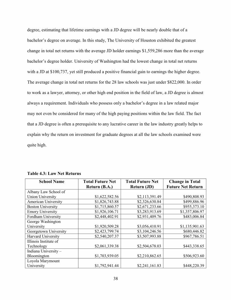
38

degree, estimating that lifetime earnings with a JD degree will be nearly double that of a

bachelor’s degree on average. In this study, The University of Houston exhibited the greatest

change in total net returns with the average JD holder earnings $1,559,286 more than the average

bachelor’s degree holder. University of Washington had the lowest change in total net returns

with a JD at $100,737, yet still produced a positive financial gain to earnings the higher degree.

The average change in total net returns for the 28 law schools was just under $822,000. In order

to work as a lawyer, attorney, or other high end position in the field of law, a JD degree is almost

always a requirement. Individuals who possess only a bachelor’s degree in a law related major

may not even be considered for many of the high paying positions within the law field. The fact

that a JD degree is often a prerequisite to any lucrative career in the law industry greatly helps to

explain why the return on investment for graduate degrees at all the law schools examined were

quite high.

Table 4.3: Law Net Returns

School Name Total Future Net Return (B.A.)

Total Future Net Return (JD)


Albany Law School of Union University $1,622,582.56 $2,113,391.49 $490,808.93 American University $1,826,743.88 $2,326,630.84 $499,886.96 Boston University $1,715,860.57 $2,671,233.66 $955,373.10 Emory University $1,926,106.71 $3,283,913.69 $1,357,806.97 Fordham University $2,448,402.91 $2,931,409.76 $483,006.84 George Washington University $1,920,509.28 $3,056,410.91 $1,135,901.63 Georgetown University $2,423,799.74 $3,104,246.56 $680,446.82 Harvard University $2,540,207.37 $3,507,993.88 $967,786.51 Illinois Institute of Technology $2,061,339.38 $2,504,678.03 $443,338.65 Indiana University – Bloomington $1,703,939.05 $2,210,862.65 $506,923.60 Loyola Marymount University $1,792,941.44 $2,241,161.83 $448,220.39

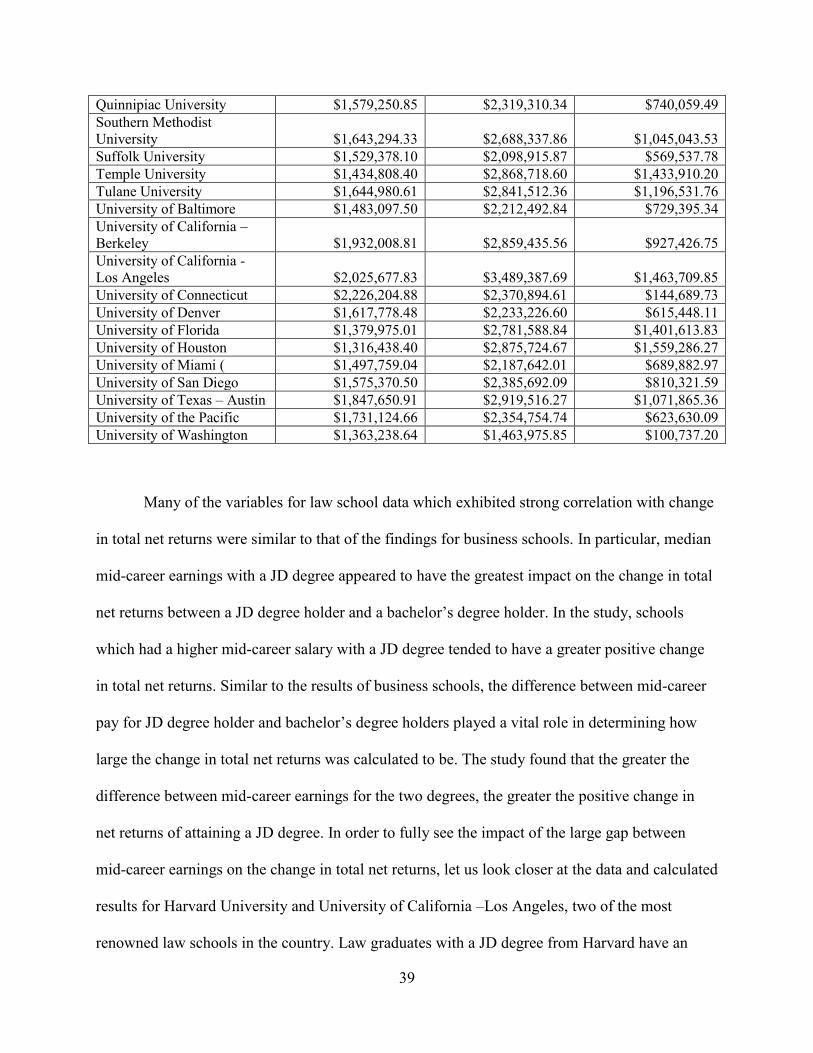
39

Quinnipiac University $1,579,250.85 $2,319,310.34 $740,059.49 Southern Methodist University $1,643,294.33 $2,688,337.86 $1,045,043.53 Suffolk University $1,529,378.10 $2,098,915.87 $569,537.78 Temple University $1,434,808.40 $2,868,718.60 $1,433,910.20 Tulane University $1,644,980.61 $2,841,512.36 $1,196,531.76 University of Baltimore $1,483,097.50 $2,212,492.84 $729,395.34 University of California – Berkeley $1,932,008.81 $2,859,435.56 $927,426.75 University of California - Los Angeles $2,025,677.83 $3,489,387.69 $1,463,709.85 University of Connecticut $2,226,204.88 $2,370,894.61 $144,689.73 University of Denver $1,617,778.48 $2,233,226.60 $615,448.11 University of Florida $1,379,975.01 $2,781,588.84 $1,401,613.83 University of Houston $1,316,438.40 $2,875,724.67 $1,559,286.27 University of Miami ( $1,497,759.04 $2,187,642.01 $689,882.97 University of San Diego $1,575,370.50 $2,385,692.09 $810,321.59 University of Texas – Austin $1,847,650.91 $2,919,516.27 $1,071,865.36 University of the Pacific $1,731,124.66 $2,354,754.74 $623,630.09 University of Washington $1,363,238.64 $1,463,975.85 $100,737.20

Many of the variables for law school data which exhibited strong correlation with change

in total net returns were similar to that of the findings for business schools. In particular, median

mid-career earnings with a JD degree appeared to have the greatest impact on the change in total

net returns between a JD degree holder and a bachelor’s degree holder. In the study, schools

which had a higher mid-career salary with a JD degree tended to have a greater positive change

in total net returns. Similar to the results of business schools, the difference between mid-career

pay for JD degree holder and bachelor’s degree holders played a vital role in determining how

large the change in total net returns was calculated to be. The study found that the greater the

difference between mid-career earnings for the two degrees, the greater the positive change in

net returns of attaining a JD degree. In order to fully see the impact of the large gap between

mid-career earnings on the change in total net returns, let us look closer at the data and calculated

results for Harvard University and University of California –Los Angeles, two of the most

renowned law schools in the country. Law graduates with a JD degree from Harvard have an

40

astounding $197,000 median mid-career salary, while UCLA is not far behind at $193,000. With

just the knowledge of this information it is reasonable to expect that Harvard would have the

higher change in net returns with a JD degree. However, bachelor’s degree holders with a social

science concentration at Harvard already have a very high median mid-career pay of $130,000

compared to $98,500 for UCLA bachelor’s degree holders. The $95,000 difference in mid-career

earnings for JD degree holder versus bachelor’s degree holders at UCLA compared to the

$67,000 difference at Harvard is a main factor in explaining why the change in net returns of a

JD degree at UCLA is actually greater, despite having a lower JD median mid-career salary. The

average wage premium for mid-career earnings with a JD degree for all schools in the study was

$60,442. Graph 4 and Graph 5 plot median mid-career earnings (JD) and difference in median

mid-career earnings against the change in total net return between a bachelor’s degree and JD

degree for the 28 schools analyzed.

Graph 4: Median Mid-Career Salary (JD)

$-

$200,000

$400,000

$600,000

$800,000

$1,000,000

$1,200,000

$1,400,000

$1,600,000

$1,800,000

$- $50,000 $100,000 $150,000 $200,000 $250,000

Cha

nge

in T

otal

Net

Ret

urns

Median Mid-Career Salary (J.D)

Series1

41

Graph 5: Difference in Mid-Career Salary (JD)

Graduate law school rankings did not appear to have any correlation with the change in total

net returns between the two degree types. Part of the reason that very little correlation was found

is likely due to the small sample of law schools in the study as well as the actual schools which

sufficient data was available for. With approximately 200 graduate law schools in the country

and only being able to gather data for 28 schools, about 85% of law schools were not considered

in the study. Additionally, only 7 of the top 25 law schools were included in the study. Further

investigation revealed that law schools rankings actually tend to be among the most important

and influential on future earnings compared to other graduate schools such as business schools.

This has much to do with the consistency of law school ranks in the past. For starters, the top 14

law schools in the nation have remained unchanged for the past 25 years from the inception of

law school rankings by U.S. News. Although the ranks among the top 14 schools have changed

slightly from year to year, they have all maintained their prestigious, unassailable reputation.

According to Forbes, the top 14 law schools (or T14) have asserted dominance such that students

$0

$200,000

$400,000

$600,000

$800,000

$1,000,000

$1,200,000

$1,400,000

$1,600,000

$1,800,000

$0 $20,000 $40,000 $60,000 $80,000 $100,000

Cha

nge

in T

otal

Net

Ret

urns

Difference Between B.A. and JD Mid Career Salary

Series1

42

covet these institutions, the best professors desire to teach at these institutions, and law firms

prioritize hiring from these institutions. If data were more complete and decisive allowing for the

inclusion of a larger number of law schools, especially those in the T14 group, law rankings

would have likely shown to be more significant in determining changes in total net returns

between bachelor’s and JD degrees.

Sensitivity analysis on the discount rate of net present value for future returns

demonstrated that results were mostly unchanged. The only changes that occurred when

adjusting the discount rate involved the degree of financial benefit that came with a JD degree, as

all the schools still demonstrated positive changes in net returns with a JD Degree. When the

discount rate was raised to 4%, the average positive change in net returns with a JD degree fell to

$643,170. Conversely, when the discount rate was dropped to 2%, the average positive change in

net returns jumped to $1,047,111. In conclusion, the sensitivity test proved that the change in net

returns with a JD degree is financially beneficial for all school included in the study with any

realistic discount rate.

Table 4.4: Sensitivity Analysis (JD)

NPV Discount Rate Avg. Change in Net Returns

# of Schools with Positive Change in

Net Returns


Net Returns 2% $1,047,111.21 28 100% 3% $821,935.98 28 100% 4% $643,170.26 28 100%

43

Section III: STEM Results

Table 4.5 illustrates the results of the change in total net returns between bachelor’s

degree and master’s degree holders from schools with a strong focus in science, technology,

engineering, and mathematics (STEM). The results for the STEM schools in this study differed

greatly from the general results for the business and law schools analyzed. As apparent in the last

column of Table 4.5, only 6 out of the 17 schools demonstrated a positive change in total net

return when pursuing a master’s degree. The 35% of STEM school that showed positive

financial gains to a master’s degree is significantly less than the 88% for Business schools and

100% for law schools observed. These findings were a bit surprising as they differed from the

results from the Bureau of Labor Statistics mentioned in Chapter 2, which found that those

working in the STEM field with a master’s degree had among the highest wage premiums at

around 25-40%. In this study, Milwaukee School of Engineering exhibited the greatest positive

change in total net returns at $167,321. At the other end of the spectrum, Case Western Reserve

University had the poorest change in total net returns with a master’s degree at -$412,386. The

average change in total net returns of obtaining a bachelor’s degree for the 17 schools was a loss

of $83,867 over a work career.

44

Table 4.5: STEM Net Returns

School Name Total Future Net Return (B.A.)

Total Future Net Return (Master’s)


Carnegie Mellon University $2,383,288.58 $2,302,504.35 ($80,784.23) Case Western Reserve University $1,845,880.57 $1,433,494.23 ($412,386.35) Clarkson University $2,332,617.88 $1,969,994.47 ($362,623.41) Colorado School of Mines $2,400,030.22 $2,423,835.90 $23,805.68 Florida Institute of Technology $1,913,291.63 $1,953,931.10 $40,639.47 Georgia Institute of Technology $2,382,042.75 $2,227,670.93 ($154,371.82) Illinois Institute of Technology $2,090,796.39 $2,029,823.10 ($60,973.29) Kettering University $2,145,649.62 $2,130,962.14 ($14,687.48) Lehigh University $2,232,526.11 $2,040,121.80 ($192,404.32) Massachusetts Institute of Technology $2,724,358.04 $2,438,421.25 ($285,936.79) Michigan Technological University $2,172,874.80 $2,214,203.68 $41,328.87 Milwaukee School of Engineering $1,885,769.12 $2,053,089.75 $167,320.63 Missouri University of Science and Technology $2,173,759.07 $2,251,751.16 $77,992.09 New Jersey Institute of Technology $2,097,474.40 $2,228,197.44 $130,723.03 Rensselaer Polytechnic Institute $2,190,457.84 $1,985,724.92 ($204,732.92) Stevens Institute of Technology $2,340,898.53 $2,218,097.31 ($122,801.22)

Worcester Polytechnic Institute $2,246,802.47 $2,230,957.68 ($15,844.79)

Although the results for STEM schools were very different than business and law

schools, some of the variables that affected the degree of change in total net returns were the

same. Again, it appeared that the difference between mid-careers salary between a bachelor’s

degree and master’s degree at a specific school played a substantial role in determining the

change in total net returns. The greater the gap between these two salaries was correlated with a

greater positive change in net returns, or in several cases, a smaller negative change in net

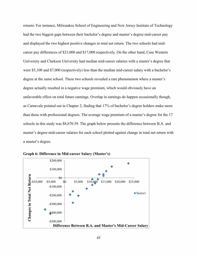
45

returns. For instance, Milwaukee School of Engineering and New Jersey Institute of Technology

had the two biggest gaps between their bachelor’s degree and master’s degree mid-career pay

and displayed the two highest positive changes in total net return. The two schools had mid-

career pay differences of $23,000 and $17,000 respectively. On the other hand, Case Western

University and Clarkson University had median mid-career salaries with a master’s degree that

were $5,100 and $7,000 (respectively) less than the median mid-career salary with a bachelor’s

degree at the same school. These two schools revealed a rare phenomenon where a master’s

degree actually resulted in a negative wage premium, which would obviously have an

unfavorable effect on total future earnings. Overlap in earnings do happen occasionally though,

as Carnevale pointed out in Chapter 2, finding that 17% of bachelor’s degree holders make more

than those with professional degrees. The average wage premium of a master’s degree for the 17

schools in this study was $8,670.59. The graph below presents the difference between B.A. and

master’s degree mid-career salaries for each school plotted against change in total net return with

a master’s degree.

Graph 6: Difference in Mid-career Salary (Master’s)

-$500,000

-$400,000

-$300,000

-$200,000

-$100,000

$0

$100,000

$200,000

-$10,000 -$5,000 $0 $5,000 $10,000 $15,000 $20,000 $25,000

Cha

nges

in T

otal

Net

Ret

urn

Difference Between B.A. and Master's Mid-Career Salary

Series1

46

Undergraduate rank of the STEM schools also showed some negative correlation with

change in total net returns. Schools which were ranked higher (closer to 1) tended to have a

lower or more negative change in total net returns with a master’s degree. For example,

Massachusetts Institute of Technology is the highest ranked undergraduate STEM school in the

study at #5 and has one of the poorest changes in total net returns at -$285,937. Alternatively,

Milwaukee School of Engineering which had the highest positive change in net returns has an

undergraduate rank of 481. The negative relationship between undergraduate institution rank and

change in total net returns is likely somewhat attributable to the previous correlation found

between differences in mid-career earnings. Schools which have prestigious undergraduate

programs likely already have high median mid-career earnings for bachelor’s degree graduates,

meaning that the wage premium of a master’s degree may not be that substantial. In the case of

MIT, the median-mid career wage premium with a master’s degree was only $3,000 a year,

mainly because the bachelor’s degree median salary was already a sizeable amount at $134,000.

Therefore, undergraduate rank and the median mid-career salaries for the different degree types

should be evaluated carefully when deciding on whether to pursue a master’s degree at a STEM

school. Graph 7 shows the relationship between undergraduate school rank and change in total

net return with a master’s degree for the observed STEM schools.

47

Graph 7: Undergraduate School Rank

The last variable which displayed correlation with change in total net return was the

master’s program tuition. Negative correlation was observed, as the financial gain to a master’s

degree became less advantageous when the tuition was higher. As observed in Chapter 2, tuition

and fees have increased tremendously in the past decade and it appears to have actually had some

effect on the returns to a master’s degree in STEM over a work career. This correlation is quite

fascinating, seeing that none of the costs (such as tuition) for business and law schools seemed to

have any significant correlation with change in total net returns. The small gap between earnings

for bachelor’s degree and master’s degree holders in STEM most likely made the costs play a

more crucial role in determining change in total net returns. Graph 8 below demonstrates the

relationship between the two variables.

-$500,000.00

-$400,000.00

-$300,000.00

-$200,000.00

-$100,000.00

$0.00

$100,000.00

$200,000.00

0 100 200 300 400 500 600

Cha

nge

in T

otal

Net

Ret

urn

Undergraduate School Rank

Series1

48

Graph 8: Master’s Program Tuition Cost

Sensitivity analysis for the STEM schools revealed that the majority of the schools still

remained having a negative change in total net returns with a master’s degree. Discounts rates of

2%, 3%, and 4% all exhibited a negative return of a master’s degree compared to a bachelor’s

degree. The only major changes with sensitivity analysis showed that with a rate of 4% the

number of schools with a positive change in net return dropped to 5, just 29% of the observed

schools. On the other hand, with a rate of 2% the number of schools exhibiting a positive change

increased to 7, still representing less than half of the schools at 41%. Table 4.6 displays the

degree of change that occurred in terms of change in total net returns using the different discount

rates tested.

Table 4.6: Sensitivity Analysis (STEM) NPV Discount Rate Avg. Change in Net

Returns # of Schools with

Positive Change in Net Returns


Net Returns 2% (77,596.35) 7 41% 3% ($83,866.87) 6 35% 4% (92,662.87) 5 29%

-$500,000.00

-$400,000.00

-$300,000.00

-$200,000.00

-$100,000.00

$0.00

$100,000.00

$200,000.00

0 20000 40000 60000 80000 100000 120000

Cha

nge

in T

otal

Net

Ret

urn

Master's Program Tuition Cost

Series1

49

Chapter Five

Conclusion

A. Summary of Results

This section highlights the key findings from the calculated results, explaining which variables had the most significant impact on the value of a master’s degree

This study found that investing in a master’s degree in business and law concentrations

provided positive total net returns compared to a bachelor’s degree. Alternatively, a master’s

degree in STEM subjects exhibited negative net returns in comparison to a bachelor’s degree in

the same academic field. Changes in median mid-career earnings between a bachelor’s degree

and master’s degree appeared to be the most influential factor in determining whether pursuing a

master’s degree was worth the cost. More specifically, the mid-career wage premium with a

master’s degree had strong correlation with the positive change in total net returns between a

bachelor’s degree and master’s degree for all three academic focuses. School rankings also

displayed some correlation with the change in total net returns of a master’s degree for business

and STEM schools. Higher ranked (closer to 1) graduate business schools were associated with

greater changes in total future earnings with a master’s degree. The quality of education, strong

alumni network, and high status reputation, of top ranked business schools are likely key

contributors to explaining why graduates from these institutions tend to earn the highest earnings

over a work career. Undergraduate ranks for STEM schools exhibited negative correlation with

positive change in total net returns of a master’s degree over a bachelor’s degree. The main

reason for this negative relationship is due to the high earnings that are already associated with a

bachelor’s degree at top ranked, prestigious undergraduate STEM schools. Therefore, students

50

who attend elite undergraduate STEM schools should be more cautious about pursuing an

advanced degree if the end goal is higher monetary gains. Additional student loan debt required

to achieve a master’s degree did not appear to significantly impact the monetary gains to a

master’s degree. Interestingly, all of the costs which were incorporated in the calculations proved

to have very little significance. Master’s degree tuition and fees for STEM schools was the only

cost variable which exhibited any correlation with the change in total net returns to a master’s

degree. Although overall when analyzing the results of all three subjects, tuition costs, student

loan amounts, and opportunity costs of a foregone salary, all had little effect on determining how

valuable a master’s degree was at the observed schools.

B. Limitations This section addresses limitations in this study, emphasizing that results are calculated for the average student, while introducing further research that could be conducted with access to certain data

The primary limitation of this study is the examination of change in total net returns at an

institutional level rather than at the individual level. Using data for median earnings and costs for

schools observed are advantageous because of their accessibility; however it inhibits the ability

to test the effects of other variables which may influence the real returns to a master’s degree.

Financial factors such as household income, student loan debt, and scholarship amount vary for

each student and could potentially play a critical role in determining whether opting to attend

graduate school is a smart investment. Full tuition and fee costs do not always accurately

represent the true price to attending a university, as the actual price may be significantly lower

due to scholarships, grants and other forms of financial aid for certain students. Other factors

51

such as race and gender may also affect the value of a master’s degree for several reasons such as

discrimination in the workforce. Using data at the school level prevents the study to measure the

correlation between these variables, which differ by individual, with the total net returns of a

master’s degree compared to a bachelor’s degree. Obtaining data for individual cases of students

holding only a bachelor’s degree and those with a master’s degree could contribute to identifying

other variables and characteristics that relate to the return on investment of a master’s degree.

Further research with the availability of data at the individual level could then potentially explain

which personal characteristics have a direct effect on the change in total net returns of attaining a

master’s degree.

Another limitation to the study was the sample size of schools, particularly for law and

STEM schools. Insufficient data prevented the PayScale 2016-2017 College Salary Report from

including median earnings for numerous schools in the report. Several prestigious graduate law

and STEM schools were excluded from this study due to the lack of verifiable earnings data.

Furthermore, many of the graduate law schools presented in the PayScale report were

independent institutions that were not associated with an undergraduate university, which

impeded on the ability to compare the net returns between a bachelor’s and master’s degree.

More accessible school data would have allowed a greater sample size and would help confirm

that these results were consistent throughout a larger number of institutions.

52

C. Concluding Remarks

This section reiterates which academic concentrations demonstrated positive changes in total net returns with a master’s degree, while also stressing the importance of personal characteristics and circumstances which may play a role in determining the returns to graduate school

It is imperative to realize that this study reveals which schools are worthy investments for

individuals who are solely interested in the monetary returns to an advanced degree. Individuals

who pursue a master’s degree with the main intent to build their human capital, expand their

knowledge, and simply further their education may be perfectly satisfied with obtaining a

master’s degree regardless of the change in total net returns associated with the advanced degree.

The financial costs and benefits to obtaining a master’s degree will differ for each individual, but

using median earnings and average costs, this study demonstrates that attending graduate school

to pursue an MBA or JD degree are typically smart financial choices. Conversely, the results of

this study would suggest avoiding graduate school for STEM subjects if monetary gains are the

primary objective of obtaining an advanced degree. For all three academic concentrations, the

difference in median mid-career earnings between bachelor’s degree and master’s degree holders

proved to be the most influential factor in determining whether a master’s degree was worth it.

Students contemplating whether to attend graduate school should carefully assess their own

financial circumstances. However, using the results of this study, individuals deciding on

whether to attend graduate school can be confident that the wage premium for master’s degree in

business and law over an entire work career will adequately compensate for the costs of

obtaining the degree, resulting in a financially advantageous investment for the average student.

53

Reference List

Avery, Christopher, and Sarah Turner (2012). “Student Loans: Do College Students Borrow Too Much—Or Not Enough?” Journal of Economic Perspectives (26) 165-192.

Berman, Jillian (2016). “America’s Growing Student-Loan-Debt Crisis.” MarketWatch.

Carnevale, Anthony (2009). “The College Payoff: Education, Occupations, Lifetime Earnings.” The Georgetown University Center on Education and the Workforce.

Delisle, Jason (2014). “The Graduate Student Debt Review: The State of Graduate Student Borrowing.” New America Education Policy.

Dynarski, Susan (2014). “An Economist’s Perspective on Student Loans in the United States”. Brookings Institute.

Dynarksi, Susan (2016). “The Trouble with Student Loans? Low Earnings, Not High Debt.” Brookings Institute.

Federal Student Aid, an Office of the Department of Education,

Foroohar, Rana (2016). “How the Financing of Colleges May Lead to Disaster!” The New York Review.

Lindley, Joanne, and Stephen Machin (2013). “The Rising Postgraduate Wage Premium.” Department of Management, King’s College London. Department of Economics, University College London and Centre for Economic Performance, London School of Economics.

Looney, Adam, and Yannelis Constantine (2015). “A Crisis in Student Loans? How Changes in the Characteristics of Borrowers and in the Institutions They Attend Contributed to Rising Loan Defaults.” Brookings Institute.

Macklin, Dan (2016). “Undergraduate VS. Graduate Student Loans: 6 Ways They Differ.” SoFi

Mitchell, Travis (2015). “Chart: See 20 Years of Tuition Growth at National Universities.” U.S News.

O’Connor, Shawn (2012). “Grad School: Still worth the Money.” Forbes

Paul, Mark, and Anastasia Wilson (2016). “Profiting off Debt.” Jacobin

Torpey, Elka, and Dalton Terell (2015). “Should I get a Master’s Degree?” Bureau of Labor Statistics.

54

"Tuition and Fees and Room and Board over Time, 1976-77 to 2016-17, Selected Years." CollegeBoard (2016).

United States Department of Education. “Federal Student Aid Data Center” (2005-2016)

Valleta, Robert (2015). “Recent Flattening in the Higher Education Wage Premium: Polarization, Deskilling, or Both?” The National Bureau of Economic Research.

Documents

Is Graduate School Worth It? Evaluating the Return on