Is Inflation Persistence Intrinsicin Industrial Economies?

Andrew T. Levin *and

Jeremy Piger **

First Draft: October 2002This Draft: February 2003

Abstract: We apply both classical and Bayesian econometric methods to characterize the dynamicbehavior of inflation for twelve industrial countries over the period 1984-2002, using four different priceindices for each country. In particular, we estimate a univariate autoregressive (AR) model for eachseries, and consider the possibility of a structural break at an unknown date. In most cases, we find strongevidence for a break in the intercept of the AR equation in the late 1980s or early 1990s, while there is noevidence of a break in any of the AR coefficients. Conditional on the break in the intercept, inflationexhibits very little persistence: for roughly 70% of the inflation series the point estimate of the sum of theAR coefficients is less than 0.7. Further, the unit root null hypothesis is rejected in nearly all of thesecases. These results indicate that high inflation persistence is not an inherent characteristic of industrialeconomies.

Keywords: Inflation dynamics, Bayesian econometrics, largest autoregressive root.JEL Codes: C11, C22, E31

We appreciate helpful comments from Nicoletta Batini, Luca Benati, Todd Clark, Günter Coenen, ChrisErceg, Luca Guerrieri, Lutz Killian, Jesper Lindé, Ming Lo, Mike McCracken, Ed Nelson, Mark Watson,Volker Wieland, Tony Yates, and seminar participants at the Bank of England, Bank of France, EuropeanCentral Bank, Federal Reserve Banks of Kansas City and St. Louis, and the University of Missouri. Weare also grateful to Chang-Jin Kim for providing Gauss code to perform the marginal likelihoodcalculations. Maura McCarthy provided excellent research assistance. The views expressed in this paperare solely the responsibility of the authors, and should not be interpreted as reflecting the views of theBoard of Governors of the Federal Reserve System, the Federal Reserve Bank of St. Louis, or of anyother person associated with the Federal Reserve System.

** Federal Reserve Board, Stop 70, Washington, DC 20551 USA phone 202-452-3541; fax 202-452-2301; email andrew.levin@frb.gov

*** Federal Reserve Bank of St. Louis, P.O. Box 442, St. Louis, MO 63166 USA phone 314-444-8718; fax 314- 444-8731; email piger@stls.frb.org

-2-

1. Introduction

A large econometric literature has found that postwar U.S. inflation exhibits very high

persistence, approaching that of a random-walk process.1 Given similar evidence for other

OECD countries, many macroeconomists have concluded that high inflation persistence is a

“stylized fact” and have proposed a number of different microeconomic interpretations.2

However, an alternative viewpoint is that the degree of inflation persistence is not an inherent

structural characteristic of industrial economies, but rather varies with the stability and

transparency of the monetary policy regime.3

In this paper, we utilize both classical and Bayesian econometric methods to characterize

the behavior of inflation dynamics for twelve industrial countries: Australia, Canada, France,

Germany, Italy, Japan, Netherlands, New Zealand, Sweden, Switzerland, the United Kingdom,

and the United States. To ensure that our results are not specific to a particular measure of

inflation, we analyze the properties of four different price indices: the GDP price deflator, the

personal consumption expenditure (PCE) price deflator, the consumer price index (CPI), and the

core CPI. We focus our analysis on the sample 1984-2002, the time period for which the degree

of inflation persistence is most disputed. Specifically, there is widespread agreement that

inflation persistence was very high over the period extending from 1965 to the disinflation of the

1 See Nelson and Plosser (1982), Fuhrer and Moore (1995), Pivetta and Reis (2001), Stock (2001).2 For further discussion, see Nelson (1998) and Clarida et al. (1999). In developing microeconomic foundations forhigh inflation persistence, some authors assume that private agents face information-processing constraints; cf.Roberts (1998), Ball (2000), Ireland (2000), Mankiw and Reis (2001), Sims (2001), Woodford (2001). Analternative approach assumes that high inflation persistence results from the structure of nominal contracts; cf.Buiter and Jewitt (1989), Fuhrer and Moore (1995), Fuhrer (2000), Calvo et al. (2001), Christiano et al. (2001).Other authors generate inflation persistence through the data generating process for the structural shocks hitting theeconomy; cf. Rotemberg and Woodford (1997), Dittmar, Gavin and Kydland (2001), Ireland (2003).3 See Bordo and Schwartz (1999), Sargent (1999), Erceg and Levin (2002), Goodfriend and King (2001).

-3-

early 1980s. However, there is substantial debate regarding whether inflation persistence

continued to be high since the early 1980s, or has declined.4

For many of the countries we consider there have been substantial shifts in monetary

policy that have occurred over the past decade, particularly the widespread adoption of explicit

inflation targets.5 Thus, a key aspect of our methodology is to allow for the possibility of a

structural break in the inflation process for each country, since a failure to account for such

breaks could yield spuriously high estimates of the degree of persistence (cf. Perron 1990). For

most countries, we find that inflation is best characterized as a low-order autoregressive (AR)

process with a single break in intercept at some point in the late 1980s or early 1990s, while

there is no evidence of a break in any of the AR coefficients.6

Conditional on a single structural break in the intercept, most of the inflation series

exhibit relatively low persistence. As in Andrews and Chen (1994), we measure the degree of

persistence of the process in terms of the sum of the AR coefficients, ρ (henceforth denoted as

the “persistence parameter”).7 We find point estimates of ρ that are less than 0.7 for 32 of the

48 inflation series considered. Further, ninety percent bootstrap confidence intervals do not

include the null hypothesis that 1=ρ for 35 of the inflation series. Evidence from Bayesian

posterior distributions for ρ yields similar conclusions.

These results indicate that high inflation persistence is not an inherent characteristic of

industrial economies. This conclusion is consistent with a growing literature documenting time-

4 Focusing on post-1984 data also allows us to avoid the effects of wage and price controls, which were common inmany industrial countries during the 1970s.5 See Bernanke et al. (1999), Johnson (2002), Mishkin and Schmidt-Hebbel (2002). 6 Our finding of a structural break in the mean inflation rate is consistent with Rapach and Wohar (2002) who findevidence of multiple structural breaks in the mean of the real interest rate and inflation rate of 13 industrializedcountries over the past 40 years.

-4-

variation in the level of U.S. inflation persistence. Barsky (1987) finds that U.S. inflation

persistence was very high from 1960-1979, but was much lower from 1947-1959. Evans and

Wachtel (1993) estimate a Markov-switching model for U.S. inflation and find that the series

was generated by a low-persistence regime (ρ = 0.58) during 1953-67 and 1983-93, but was

generated by a random-walk process (ρ = 1) during the period 1968-82.8 Similarly, Brainard and

Perry (2000), Taylor (2000), and Kim et al. (2001) find evidence that U.S. inflation persistence

during the Volcker-Greenspan era has been substantially lower than during the previous two

decades, while Cogley and Sargent (2001) conclude that U.S. inflation persistence reached a

postwar peak around 1979-80. International evidence includes Ravenna (2000), who documents

a large post-1990 drop in Canadian inflation persistence and Benati (2002), who finds that U.K.

and U.S. inflation had no persistence during the metallic-standard era (prior to 1914), maximum

persistence during the 1970s, and markedly lower persistence during the past decade. 9

The remainder of this paper is organized as follows. Section 2 considers naive estimates

of inflation persistence obtained without any consideration of structural breaks. Section 3 lays

out the techniques used to evaluate the evidence for structural breaks in the inflation data, while

Section 4 presents the results obtained from these techniques. Section 5 evaluates the degree of

inflation persistence conditional on structural breaks. Section 6 summarizes our conclusions and

outlines several issues for further research.

7 As noted by Andrews and Chen (1994), ρ is monotonically related to the cumulative impulse response of the seriesand to its spectral density at frequency zero, and is more informative than the largest AR root as a measure of overallpersistence. 8 These shifts in the persistence of U.S. inflation correspond reasonably well to shifts in the monetary policy regime:Romer and Romer (2002) emphasize the extent to which U.S. monetary policy was successful in stabilizing inflationduring the 1950s, while Clarida et al. (2000) consider the period after 1965 and find evidence for a shift in monetarypolicy at the beginning of the Volcker-Greenspan era.9 In contrast, Pivetta and Reis (2001) and Stock (2001) find no evidence of shifts in inflation persistence in postwarU.S. data, while Batini (2002) finds relatively little evidence of shifts in inflation persistence in Euro area countries.

-5-

2. Naive Estimates of Persistence

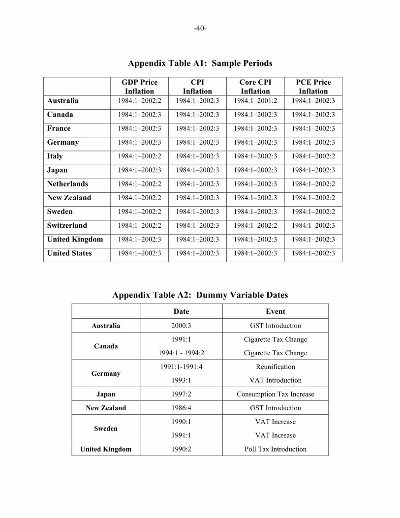
Figure 1 depicts the four inflation series for each country over the sample period 1984

through 2002; the precise sample period for each series is indicated in Appendix Table A1.10

The core CPI inflation measures exclude both food and energy prices for all countries except

Australia, for which only food prices are excluded.

Broadly speaking, Figure 1 indicates that all four inflation series tend to move roughly in

parallel. Of course, there are some exceptions; for example, the sudden drop in global oil prices

in 1986 typically has a much larger impact on consumer inflation than on GDP price inflation.

We have also identified a few specific cases in which exogenous events, such as shifts in VAT or

other sales tax rates, resulted in large transitory fluctuations in the inflation series. The dates of

these events are listed in Appendix Table A2. As shown by Franses and Haldrup (1994), such

outliers can induce substantial downward bias in the estimated degree of persistence. Thus, we

replace these outliers with interpolated values (the median of the six adjacent observations that

were not themselves outlier observations).

If one ignores the possibility of structural breaks, then Figure 1 suggests that most of

these countries have a fairly high degree of inflation persistence. For example, Australian GDP

price inflation has a mean value of about 3.6 percent over the period 1984-2002, but the series is

consistently higher than this value prior to 1991 and then consistently falls below the mean

during the later years of the sample. Similar patterns are apparent for Canada, New Zealand,

Sweden, the United Kingdom, and the United States: in each case, inflation largely remains

above its sample mean during the 1980s and thereafter tends to remain below the mean.

10 All data was collected from the OECD Statistical Compendium. Data availability determined the terminal date ofthe sample for each inflation series, which differs across countries and inflation measures. It should be noted thatthe German series do not include any data for 1991, since these series have been constructed by splicing togetherpost-1992 data for unified Germany with pre-1991 data for West Germany.

-6-

To formalize these impressions, we now consider a univariate AR process for each

inflation series:

∑ ++==

−K

jtjtjt

1επαµπ (1)

where tε is a serially uncorrelated but possibly heteroscedastic random error term. To measure

the degree of persistence in terms of the sum of AR coefficients, it is useful to reexpress the

equation as follows:

∑ +++=−

=−−

1

11

K

jtjtjtt επ∆φρπµπ (2)

where the persistence parameter ∑≡ jαρ , and the higher-order dynamic parameters φj are

simple transformations of the AR coefficients in equation (1); e.g., KK αφ −=−1 . Note that if

1=ρ , the process has a unit root. Alternatively, if the data-generating process is stationary, then

the parameter ρ is less than unity and serves as a useful indicator of the degree of persistence of

the process (cf. Andrews and Chen 1994).

To obtain a particular estimate of ρ , an AR lag order K must be chosen for each inflation

series. For this purpose, we utilize AIC, the information criterion proposed by Akaike (1973),

with a maximum lag order of K = 5 considered. The lag order chosen for each series is reported

in Appendix Table A3. While not reported here, we have found that using SIC (the criterion

proposed by Schwarz 1978) does not alter any of the conclusions reached in this paper.

It is well known that the least-squares estimator of the persistence parameter ρ , denoted

ρ̂ , is biased downward, particularly as ρ approaches unity. Further, confidence intervals

constructed based on an asymptotic normal distribution for ρ̂ do not have correct coverage. To

-7-

remedy these deficiencies with the standard estimation techniques, we construct confidence

intervals using the “grid bootstrap” procedure of Hansen (1999), which simulates the sampling

distribution of the t-statistic )ˆ(

ˆρρρ

set −= over a grid of possible true values for ρ in order to

construct confidence intervals with correct coverage. In the bootstrap procedure we allow for

heteroscedasticity by constructing )ˆ(ρse using the White (1980) heteroscedasticity-consistent

standard error estimator and scaling each of the parametrically generated bootstrap residuals by

the actual residual obtained from least-squares estimation of equation (2) conditional on each

value of ρ in the grid. This is important as many of the inflation series considered here are

much less volatile over the second half of the sample period.

The results broadly support the view that high inflation persistence is a “stylized fact” of

industrialized economies. Table 1 reports the 5th , 50th and 95th percentiles of the bootstrap

confidence intervals for ρ . Figure 2 displays this same information graphically. The 95th

percentile estimate exceeds unity for 40 of the 48 inflation series, that is, the unit root null

hypothesis cannot be rejected for these series at the 5% level. The median estimate typically

exceeds 0.7, and is 0.85 or greater for well over half of the cases considered. Thus, based on

these estimates, a reasonable conclusion is that high inflation persistence is pervasive across

countries and measures of inflation.11

11 Table 1 highlights the importance of considering several alternative measures of inflation when evaluatinginflation persistence for any particular country. For example, the U.S. inflation data, as measured by the GDP pricedeflator, PCE price deflator, and core CPI, is consistent with high persistence – the median estimates of ρ are

-8-

3. Methodology for Identifying Structural Breaks

As demonstrated by Perron (1990), the degree of persistence of a given time series will

be exaggerated if the econometrician fails to recognize the presence of a break in the mean of the

process. Thus, before drawing any firm conclusions about inflation persistence from the results

in the previous section, it is important to obtain formal econometric evidence about the presence

or absence of structural breaks in these series. In this section, we present the classical and

Bayesian methodology used to evaluate the evidence for structural breaks.

3.1 General Specification

We begin by reformulating equation (2) to allow for a single shift in the intercept:

∑ ++++=−

=−−

1

1110

K

jtjtjttt D επ∆φρπµµπ (3)

where the dummy variable Dt equals zero in periods t < s and equals unity in all subsequent

periods t ≥ s. As discussed below, we have also considered the possibility of structural breaks in

the AR coefficients, but find no evidence of such breaks. As before, tε is a serially uncorrelated

but possibly heteroscedastic random error term.

For each inflation series, we consider a structural break without making any assumptions

about the specific break date, s. If one possessed a priori knowledge of the break date, then one

could simply estimate equation (2) over the two subsamples and then apply the breakpoint test of

Chow (1960). For the data considered here, however, the appropriate break date is not

necessarily obvious. During the first half of the 1990s, inflation-targeting regimes were

implemented by five countries (Australia, Canada, New Zealand, Sweden, and the United

above 0.7 and the 95th percentile estimates are near or exceeds unity. However, total CPI inflation appears much

-9-

Kingdom), but the timing of any break in the inflation process need not have coincided precisely

with the formal adoption date. Furthermore, four other countries (France, Germany, Italy, and

the Netherlands) were oriented towards meeting the Maastricht criteria and hence experienced

converging inflation rates during the period leading up to European Monetary Union.

3.2 Classical Analysis

We test for a break in the intercept at an unknown break date using the Quandt (1960)

test statistic, the maximum value of the Chow test statistic obtained from searching over all

candidate break dates. The lag order K is set equal to the lag length chosen by the AIC for the

model with no structural break (reported in Appendix Table A3). To obtain an asymptotic p-

value for this statistic we use the “fixed-regressor” bootstrap procedure of Hansen (2000),

allowing for heteroscedasticity under the null hypothesis by scaling each of the parametrically

generated bootstrap residuals by the actual residual obtained from least-squares estimation of

equation (3). Alternatively, we could use the asymptotic critical values derived in

Andrews (1993). We prefer the Hansen procedure because the Andrews critical values are not

robust to structural change in the marginal distribution of the regressors, a case that is of interest

in the AR models we consider here. In implementing this procedure, we assume that the break

did not occur during the initial 15 percent nor the final 15 percent of the sample period (that is,

about ten quarters at either end of the sample). For those series for which the Hansen procedure

yields a p-value less than 0.10, we also compute the least-squares estimate of the break date, that

is the break date than minimized the sum of the squared estimated residuals.12

less persistent, with a median estimate equal to 0.51 and a 95th percentile estimate far below unity.12 See Bai (1994, 1997) for the theory of least-squares break date estimation.

-10-

3.3 Bayesian Model Comparison

As an alternative perspective to the hypothesis tests, we also investigate the evidence of a

structural break in the intercept at an unknown date using a formal Bayesian model comparison.

This can be performed using the log Bayes Factor, ln(BF), that is, the difference between the log

marginal likelihood associated with equation (3) and the log marginal likelihood of equation

(2).13 If the model with a break in the intercept is preferred to that with no structural change

ln(BF) is positive.

To calculate the likelihood function necessary for the marginal likelihood calculations the

models in equations (2) and (3) need to be more fully specified. First, we must place restrictions

on the distribution and variance-covariance matrix of the residuals. We assume that the residual

in equation (2) and (3), tε is serially independent and has a Gaussian distribution with mean zero

and variance 2iσ . We model potential heteroscedasticity in tε by allowing for a one time

structural break in the variance of the residuals, that is )()1( 21

20

2tti DD σσσ +−= . For the

model in equation (3), tD controls the shift in the intercept and in the innovation variance, thus

the breaks are constrained to occur at the same time. We must also place some structure on the

unobserved dummy variable tD for construction of the likelihood function. To this end we

follow Chib (1998) in assuming that Dt is a discrete latent variable with Markov transition

probabilities Pr(Dt+1 = 0 |Dt = 0 ) = q and Pr(Dt+1 = 1 |Dt = 1 ) = 1, where 0 < q < 1. In any

period in which the break has not yet occurred (that is, Dt = 0), there exists a constant non-zero

probability q−1 that the break will occur in the subsequent period (Dt+1 = 1). Thus, the

13 The marginal likelihood of each model is obtained by computing the integral (over the entire parameter space) ofthe product of the likelihood function and the prior density function. We follow Chib (1995) in computing themarginal likelihood based on output from the Gibbs-sampling procedure.

-11-

expected duration of the number of periods prior to the break is given by E(s) = 1/(1-q). Finally,

once the break occurs at a specific date s, we have Dt = 1 for all t ≥ s.

We specify fairly diffuse prior distributions for the model parameters. In particular, we

assume that the parameter vector {µ0, µ1, ρ, φ1, …, φK-1} has a Gaussian prior distribution with

mean ......,0} 0, 0,1, ,0{ and variance-covariance matrix I*3 , while the parameters σ20 and σ2

1

each have an inverted Gamma(1,2) prior distribution and the transition probability parameter q

has a Beta(8, 0.05) prior distribution. The lag order K was chosen as the value of K that

maximized the marginal likelihood for the model under consideration, with the largest value of K

considered equal to 5.

As in Kim and Nelson (1999), we estimate this model using the Gibbs sampler, a

Markov-Chain Monte Carlo simulation technique that simulates draws from the joint parameter

posterior distribution for the model in question. Through repeated draws from this distribution,

the features of the posterior distribution (such as the mean and variance) can be approximated to

an arbitrary degree of accuracy.14 Consistent with the classical tests, we constrain the break date

to occur in the middle 70% of the sample. This is achieved by rejecting all draws from the

posterior distribution that include break dates in the first or last 15% of the sample.

3.4 Structural Breaks in the Autoregressive Parameters

Using the Bayesian procedures outlined in Section 3.3, we also consider the possibility

that a structural break occurs in the AR parameters in addition to the intercept and residual

variance. To do this, we first augment equation (3) to allow for structural change in all of the

autoregressive parameters:

14 For further details on implementing the Gibbs sampler, see Kim and Nelson (1998, 1999).

-12-

( ) ( )∑ ++++++=−

=−−

1

1111010

K

jtjtjtj0tttt DDD επ∆φφπρρµµπ (4)

Of course, for those inflation series for which K is large, a significant loss of power in detecting

structural change in the AR parameters could result due to the large number of extra parameters

that are added to equation (4) over equation (3). Thus, we also estimate a model in which a

structural break is observed only in the persistence parameter, ρ :

( ) ∑−

=−− +∆++++=

1

111010

K

jtjtjtttt DD επφπρρµµπ (5)

In both equations (4) and (5) the break in the autoregressive parameters is controlled by the

variable tD , and is thus constrained to occur at the same time as that in the intercept and residual

variance.

To compare the models with a break in the autoregressive parameters, intercept and

residual variance to the model with a break in intercept and residual variance only, we form the

log Bayes Factor, ln(BF), comparing equations (4) and (5) to equation (3). Positive values of

ln(BF) suggest the models with a break in the AR parameters are preferred. The parameter

vector {µi, ρi, φi1, …, φi,K-1 ; i = 0, 1} is assumed to have a Gaussian prior distribution with mean

0......,0} 1, 1, 0, ,0{ and variance-covariance matrix I*3 . The other prior distributions remain the

same as in Section 3.3. The lag order selection was also performed as described in Section 3.3.

4. Evidence of Structural Breaks

The results from the classical tests and Bayesian model comparison described in the

previous section are remarkably uniform in revealing structural shifts in inflation around the

early 1990s. For each country and inflation series, Table 2 records the p-value of the null

-13-

hypothesis of no structural break in the intercept of equation (3) while Table 3 records the log

Bayes Factor, ln(BF), for the comparison of equation (3) to equation (2). Again, positive values

of ln(BF) suggest the model with a break in intercept is preferred to the model with no break in

intercept.15. Beginning with the classical tests, the null hypothesis of no structural break is

rejected at the 10% level for 35 of the 48 inflation series considered. The evidence is strongest

for Australia, Canada, Italy, the Netherlands, New Zealand, Sweden, the United Kingdom, and

the United States – for each of these the null hypothesis of no structural change is rejected at the

10% level for at least three of the four inflation measures. It is interesting to note that the

evidence of a shift in intercept is very strong even for the United States, which did not adopt

explicit inflation targeting or join a currency union during the 1990s. The evidence is weakest

for Germany and Japan, where the null hypothesis is rejected for only a single inflation series,

the German GDP deflator. For the remaining two countries, France and Switzerland, the null

hypothesis is rejected for two of each country’s four measures of inflation.

The evidence from the Bayesian model comparison is very consistent with that from the

classical tests. The model with a structural break is preferred to the model with no structural

break for all four measures of inflation for Australia, Canada, Italy, the Netherlands, New

Zealand, Sweden, the United Kingdom, and the United States, while the evidence is weaker for

France, Switzerland and Germany. The primary difference is Japan, for which the classical tests

fail to reject the null hypothesis of no structural change for three measures of inflation, but the

Bayesian model comparison prefers the model with a structural break for three measures of

inflation.

15 To interpret the magnitude of ln(BF) note that, assuming a prior odds ratio of one, )(BFlne measures theposterior odds ratio. Thus, a value of ln(BF) greater than 0.7 indicates that the model with a break in intercept isdeemed to be twice as likely as the model with no break in intercept.

-14-

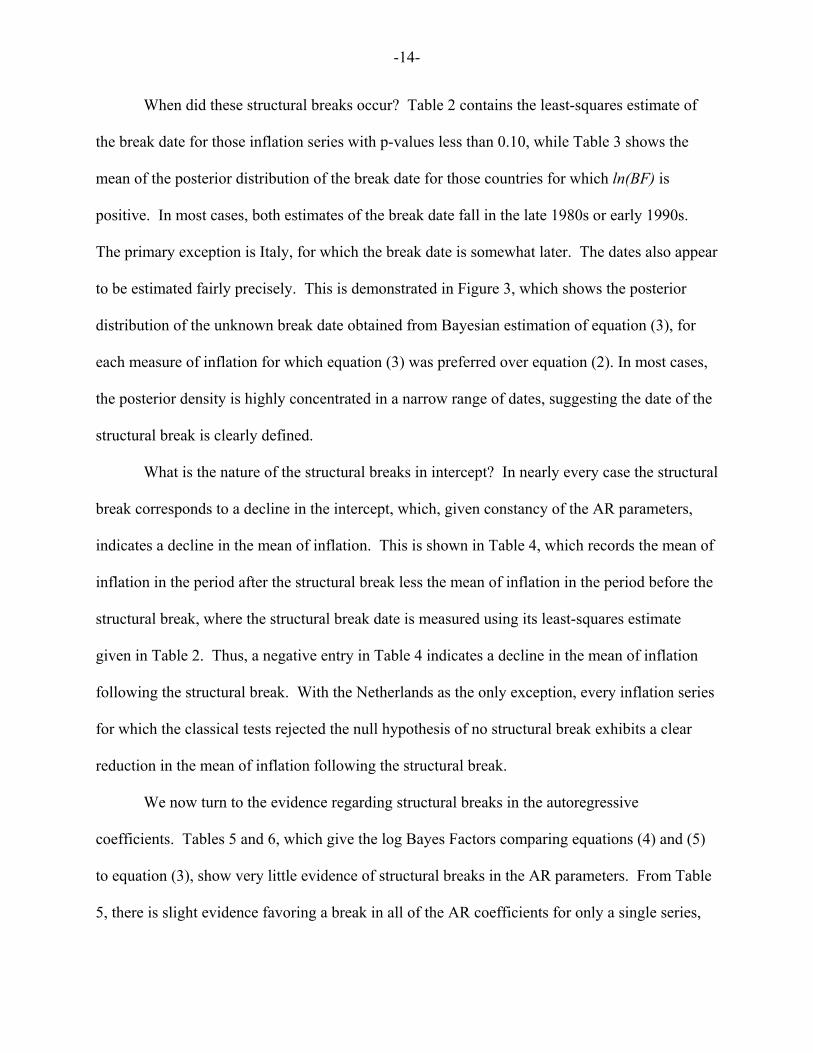
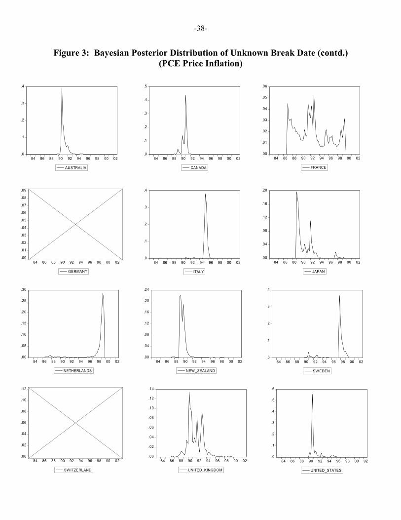
When did these structural breaks occur? Table 2 contains the least-squares estimate of

the break date for those inflation series with p-values less than 0.10, while Table 3 shows the

mean of the posterior distribution of the break date for those countries for which ln(BF) is

positive. In most cases, both estimates of the break date fall in the late 1980s or early 1990s.

The primary exception is Italy, for which the break date is somewhat later. The dates also appear

to be estimated fairly precisely. This is demonstrated in Figure 3, which shows the posterior

distribution of the unknown break date obtained from Bayesian estimation of equation (3), for

each measure of inflation for which equation (3) was preferred over equation (2). In most cases,

the posterior density is highly concentrated in a narrow range of dates, suggesting the date of the

structural break is clearly defined.

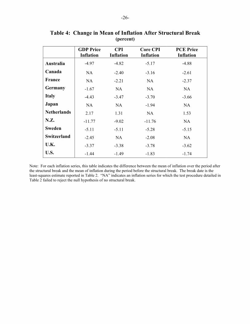
What is the nature of the structural breaks in intercept? In nearly every case the structural

break corresponds to a decline in the intercept, which, given constancy of the AR parameters,

indicates a decline in the mean of inflation. This is shown in Table 4, which records the mean of

inflation in the period after the structural break less the mean of inflation in the period before the

structural break, where the structural break date is measured using its least-squares estimate

given in Table 2. Thus, a negative entry in Table 4 indicates a decline in the mean of inflation

following the structural break. With the Netherlands as the only exception, every inflation series

for which the classical tests rejected the null hypothesis of no structural break exhibits a clear

reduction in the mean of inflation following the structural break.

We now turn to the evidence regarding structural breaks in the autoregressive

coefficients. Tables 5 and 6, which give the log Bayes Factors comparing equations (4) and (5)

to equation (3), show very little evidence of structural breaks in the AR parameters. From Table

5, there is slight evidence favoring a break in all of the AR coefficients for only a single series,

-15-

namely German PCE inflation. From Table 6, the model with a break in the persistence

parameter, ρ , but not the other AR coefficients, is the preferred model for only five measures of

inflation: Canadian CPI inflation, German PCE inflation, Italian GDP inflation, New Zealand

PCE inflation and Swiss CPI inflation. Thus, for most of the inflation series considered, the

preferred model does not include breaks in the AR parameters.

5. Reconsidering the Degree of Persistence

Having found evidence of a structural break in the mean of inflation for many of the

countries considered we now proceed to reconsider the degree of inflation persistence in these

countries.

5.1 Bootstrap OLS Estimates

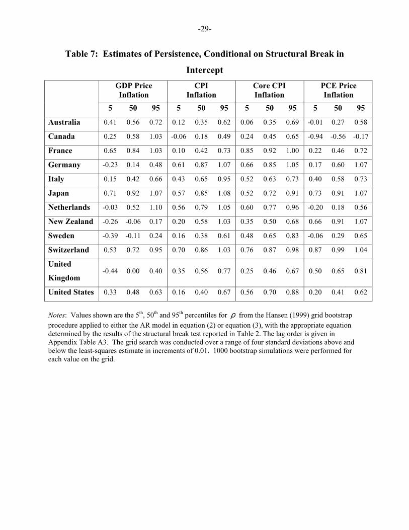
We start by taking a classical perspective, treating the break date s as known and fixed at

the date associated with its least-squares estimate (as indicated in Table 2), and using the Hansen

(1999) procedure described in Section 2 to calculate confidence intervals for ρ in equation (3).

The lag order K is chosen using the AIC (reported in Appendix Table A3). For each inflation

series for which the structural break test reported in Table 2 rejected the null hypothesis of no

structural change at the 10% level, Table 7 reports the 5th, 50th and 95th percentiles of the

confidence interval for ρ , conditional on the structural break in intercept.16 For those series

where the structural break test in Table 2 did not reject at the 10% level, Table 7 repeats the

percentiles for the model with no break in intercept reported in Table 1. Figure 4 presents this

same information graphically.

16 The lag order, K was selected using the AIC and is reported in Appendix Table A3.

-16-

In general, the estimates of inflation persistence in Table 7 are markedly lower than the

naive estimates reported in Table 1. The 95th percentile estimate is below unity for 33 of the 48

inflation series considered. By contrast, only 8 of the confidence intervals in Table 1 exclude

unity. Further, the median estimate is less than 0.7 for 32 of the 48 inflation series, as opposed to

only 5 using the naive estimate. In fact, rather than exhibiting high inflation persistence, Table 7

reveals that a number of inflation series display virtually no inflation persistence. Nearly half of

the inflation series considered having a median estimate of ρ less than 0.5, indicating that the

typical inflation fluctuation only lasts for one or two quarters.

Turning to individual countries, the results strongly suggest that inflation persistence is

quite low in Australia, Canada, Italy, Sweden, the United Kingdom and the United States. For

these countries, the median estimate of ρ is at or below 0.7 in all cases and the unit root null is

rejected for all inflation series with the exception of Canadian GDP inflation. U.S. inflation

persistence, which has received substantial attention in the existing literature, is estimated to be

very low – the upper bound of the confidence interval, that is the 95th percentile estimate, is

below 0.7 for three of the four inflation measures, and below 0.9 for all four inflation measures.

Also, the median estimate is below 0.5 for all inflation measures except the core CPI, for which

the median estimate is 0.7. The evidence is more mixed for French and New Zealand inflation.

For each of these countries, two of the inflation series appear relatively persistent – the unit root

null hypothesis cannot be rejected, while the other two series display relatively little persistence

– the unit root null hypothesis can be rejected and the median estimates of ρ are at or below 0.5.

The remaining countries, Germany, Japan, the Netherlands and Switzerland, display more

evidence of high inflation persistence.

-17-

5.2 Bayesian Estimates

The estimates in Section 5.1 were conditional on a fixed break date set equal to the least-

squares estimate of the break date. When we take a Bayesian perspective, we can evaluate the

posterior distribution of the model parameters conditional on the existence of a structural break,

without making any assumption about the specific break date; that is, the posterior distribution of

the parameter estimates is consistent with the posterior distribution of the break date.

For each inflation series for which the Bayesian model comparison in Table 3 preferred

the model with a structural break, Table 8 reports the 5th, 50th and 95th percentile of the posterior

distribution of the persistence parameter ρ obtained from estimation of equation (3). For those

inflation series for which the Bayesian model comparison preferred the model with no structural

break, Table 8 reports estimates of ρ from Bayesian estimation of equation (2). The lag order K

was chosen as the value of K that maximized the marginal likelihood, with the largest value of K

considered equal to 5. The estimates in Table 8 are consistent with those reported in Table 7,

and support the conclusion that high inflation persistence is not a stylized fact of industrialized

economies. Indeed, the Bayesian posterior distributions for ρ are suggestive of even less

inflation persistence than the classical estimates – only 12 of the 48 inflation series have a

posterior median for ρ exceeding 0.7, and only 2 series have more than 5% of the posterior

distribution for ρ above unity. This suggests that the broad finding of low inflation persistence

is reasonably robust to the estimation method; i.e., the key results are not dependent on whether

we specify a prior distribution for the break date or simply assume that the date is known and

fixed.

-18-

6. Summary and Conclusions

In this paper, we have applied classical and Bayesian econometric methods to estimate

univariate AR models of inflation for twelve industrial countries over the period 1984-2002,

using four different price indices for each country. In most cases, we find strong evidence for a

single break in the intercept, while finding no evidence of a break in any of the AR coefficients.

Conditional on the break in mean, inflation exhibits very little persistence: for roughly 70% of

the inflation series considered the point estimate of the sum of the AR coefficients is less than

0.7. Further, the unit root null hypothesis is rejected in nearly all of these cases. These results

indicate that high inflation persistence is not an inherent characteristic of industrial economies.

In future work, we intend to use these techniques in a multivariate setting, enabling us to

analyze the extent to which shifts in monetary policy regime (e.g., the adoption of inflation

targeting) has influenced the dynamic behavior of output as well as inflation. It will also be

interesting to apply these techniques to structural models of wage and price setting, thereby

helping to disentangle the extent to which estimates of high inflation persistence has been

confounded by occasional shifts in the monetary policy regime.

-19-

References

Akaike, H., 1973. Information Theory and an Extension of the Maximum Likelihood Principle.In Petrov, B., Csaki, F., eds., Second International Symposium on Information Theory.Budapest: Akademia Kiado, 267-281.

Andrews, D., 1993. Tests for Parameter Instability and Structural Change with UnknownChange Point. Econometrica 61, 821-856.

Andrews, D., and W.K. Chen, 1994, Approximately Median-Unbiased Estimation ofAutoregressive Models. Journal of Business and Economic Statistics 12, 187-204.

Bai, J., 1994. Least Squares Estimation of a Shift in Linear Processes. Journal of Time SeriesAnalysis 15, 453-72.

Bai, J., 1997. Estimation of a Change Point in Multiple Regression Models. The Review ofEconomics and Statistics 79, 551-563.

Ball, L., 2000. Near-Rationality and Inflation in Two Monetary Regimes. National Bureau ofEconomic Research Working Paper 7988.

Barsky, R.B., 1987. The Fisher Hypothesis and the Forecastibility and Persistence of Inflation.Journal of Monetary Economics 19, 3-24.

Batini, N., 2002. Euro Area Inflation Persistence. Manuscript. Bank of England.

Benati, L., 2002. Investigating Inflation Persistence Across Monetary Regimes. Manuscript,Bank of England.

Bernanke, B., Laubach, T., Mishkin, F., Posen, A., 1999. Inflation Targeting: Lessons from theInternational Experience. Princeton, NJ: Princeton University Press.

Bordo, M., Schwartz, A., 1999. Under What Circumstances, Past and Present, HaveInternational Rescues of Countries in Financial Distress Been Successful? Journalof International Money and Finance 18, 683-708.

Brainard, W., Perry, G., 2000. Making Policy in a Changing World. In Perry, G.,Tobin, J., eds., Economic Events, Ideas, and Policies: The 1960s and After.Washington, DC: Brookings Institution.

Buiter, W., Jewett, I., 1989. Staggered Wage Setting and Relative Wage Rigidities: Variations ona Theme of Taylor. Reprinted in: Willem Buiter (ed.), Macroeconomic Theory and StabilizationPolicy. University of Michigan Press, Ann Arbor, 183-199.

-20-

Calvo, G., Celasun, O., Kumhof, M., 2001. A Theory of Rational Inflationary Inertia.Manuscript, University of Maryland.

Chib, S., 1995. Marginal Likelihood from the Gibbs Output. Journal of the American StatisticalAssociation 90, 1313-1321.

Chib, S., 1998. Estimation and Comparison of Multiple Change-Point Models. Journal ofEconometrics 86, 221-241.

Chow, G., 1960. Tests of Equality Between Sets of Coefficients in Two Linear Regressions.Econometrica 28, 591-605.

Christiano, L., Eichenbaum, M., Evans, C., 2001. Nominal Rigidities and the Dynamic Effectsof a Shock to Monetary Policy. National Bureau of Economic Research Working Paper 8403.

Clarida, R., Gali, J., Gertler, M., 1999. The Science of Monetary Policy: A New KeynesianPerspective. Journal of Economic Literature 37, 1661-1707.

Clarida, R., Gali, J., Gertler, M., 2000. Monetary Policy Rules and Macroeconomic Stability:Evidence and Some Theory. Quarterly Journal of Economics 115, 147-180.

Cogley, T., Sargent, T., 2001. Evolving Post-World War II U.S. Inflation Dynamics. NBERMacroeconomics Annual 2001, 331-372.

Dittmar, R., Gavin, W., Kydland, F., 2001, Inflation Persistence and Flexible Prices. FederalReserve Bank of St. Louis Working Paper.

Erceg, C., Levin, A., 2002. Imperfect Credibility and Inflation Persistence. Forthcoming,Journal of Monetary Economics.

Evans, M., Wachtel, P., 1993. Inflation Regimes and the Sources of Inflation Uncertainty.Journal of Money, Credit, and Banking 25, 475-511.

Franses, P.H. and N. Haldrup, 1994. The Effects of Additive Outliers on Tests for Unit Rootsand Cointegration. Journal of Business and Economic Statistics, 12, 471-478.

Fuhrer, J., 2000. Habit Formation in Consumption and its Implications for Monetary PolicyModels. American Economic Review 90, 367-390.

Fuhrer, J., Moore, G., 1995. Inflation Persistence. Quarterly Journal of Economics110, 127-159.

Goodfriend, M., King, R., 2001. The Case for Price Stability. National Bureau of EconomicResearch Working Paper 8423.

-21-

Hansen, B.E., 1999. Testing for Structural Change in Conditional Models. Journal ofEconometrics 97, 93-115.

Hansen, B.E., 2000. The Grid Bootstrap and the Autoregressive Model. The Review ofEconomics and Statistics 81, 594-607.

Ireland, P., 2000. Expectations, Credibility, and Time-Consistent Monetary Policy.Macroeconomic Dynamics 4, 448-466.

Ireland, P., 2003. A Method for Taking Models to the Data. Manuscript, Boston College.

Johnson, D.R., 2002. The Effect of Inflation Targeting on the Behavior of Expected Inflation:Evidence from an 11 Country Panel. Journal of Monetary Economics 49, 1493-1519.

Kim, C., Nelson, C., 1998. State-Space Models with Regime Switching: Classical and Gibbs-Sampling Approaches with Applications. Cambridge: MIT Press.

Kim, C., Nelson, C., 1999. Has the U.S. Economy Become More Stable? A Bayesian ApproachBased on a Markov-Switching Model of the Business Cycle. Review of Economics and Statistics81, 608-616.

Kim, C., Nelson, C., Piger, J., 2001. The Less-Volatile U.S. Economy: A BayesianInvestigation of Timing, Breadth, and Potential Explanations. Manuscript, Federal ReserveBank of St. Louis.

Mankiw, N.G., Reis, R., 2001. Sticky Information Versus Sticky Prices: A Proposal to Replacethe New Keynesian Phillips Curve. NBER Working Paper 8290.

Mishkin, F., Schmidt-Hebbel, K., 2002. One Decade of Inflation Targeting in the World: WhatDo We Know and What Do We Need to Know? In Loayza, N., Soto, R., eds., A Decade ofInflation Targeting in the World. Central Bank of Chile, 117-219.

Nelson, C., Plosser, C., 1982. Trends and Random Walks in Macroeconomic Time Series:Some Evidence and Implications. Journal of Monetary Economics 10, 129-162.

Nelson, E., 1998. Sluggish Inflation and Optimising Models of the Business Cycle. Journal ofMonetary Economics 42, 303-322.

Perron, P., 1990. Testing for a Unit Root in a Time Series with a Changing Mean. Journal ofBusiness and Economic Statistics 8, 153-162.

Pivetta, F., Reis, R., 2001. The Persistence of Inflation in the United States. Manuscript,Harvard University.

Quandt, R., 1960. Tests of the Hypothesis that a Linear Regression Obeys Two SeparateRegimes. Journal of the American Statistical Association 55, 324-330.

-22-

Rapach, D.E. and M.E. Wohar, 2002. Regime Changes in International Real Interest Rates: AreThey a Monetary Phenomenon? Manuscript, University of Nebraska at Omaha.

Ravenna, F., 2000. The Impact of Inflation Targeting in Canada: A Structural Analysis.Manuscript, New York University.

Roberts, J., 1998. Inflation Expectations and the Transmission of Monetary Policy. Finance andEconomics Discussion Paper no. 98-43. Washington, D.C.: Board of Governors of the FederalReserve System.

Romer, C., Romer, D., 2002. A Rehabilitation of Monetary Policy in the 1950s. NationalBureau of Economic Research Working Paper 8800.

Rotemberg, J.J., Woodford, M., 1997. An Optimization-Based Econometric Model for theEvaluation of Monetary Policy. NBER Macroeconomics Annual 1997, 297-346.

Sargent, T., 1999. The Conquest of American Inflation. Princeton University Press.

Schwarz, G., 1978. Estimating the Dimension of a Model. Annals of Statistics 6, 461-464.

Sims, C., 2001. Implications of Rational Inattention. Manuscript, Princeton University.

Stock, J., 2001. Comment on Evolving Post-World War II U.S. Inflation Dynamics. NBERMacroeconomics Annual 2001, 379-387.

Taylor, J., 2000. Low Inflation, Pass-Through, and the Pricing Power of Firms. EuropeanEconomic Review 44, 1389-1408.

White, H., 1980. A Heteroscedasticity-Consistent Covariance Matrix Estimator and a DirectTest for Heteroscedasticity. Econometrica 48, 817-838.

Woodford, M., 2001. Imperfect Common Knowledge and the Effects of Monetary Policy.National Bureau of Economic Research Working Paper 8673.

-23-

Table 1: Estimates of Persistence, Excluding Structural Breaks

GDP PriceInflation

CPIInflation

Core CPIInflation

PCE PriceInflation

5 50 95 5 50 95 5 50 95 5 50 95Australia 0.77 1.00 1.12 0.71 0.87 1.04 0.69 0.85 1.04 0.81 1.01 1.08

Canada 0.25 0.58 1.03 0.63 0.85 1.06 0.80 0.99 1.08 0.52 0.76 1.03

France 0.65 0.84 1.03 0.51 0.71 0.9 0.85 0.92 1.00 0.57 0.75 0.94

Germany 0.49 0.73 1.01 0.61 0.87 1.07 0.66 0.85 1.05 0.17 0.60 1.07

Italy 0.70 0.88 1.04 0.75 0.89 1.02 0.80 0.87 0.95 0.80 0.9 1.00

Japan 0.71 0.92 1.07 0.57 0.85 1.08 0.83 0.93 1.01 0.73 0.91 1.07

Netherlands -0.03 1.05 1.21 0.61 0.96 1.11 0.60 0.77 0.96 0.14 0.61 1.11

New Zealand 0.35 0.61 0.9 0.70 0.89 1.05 0.72 0.9 1.05 0.66 0.91 1.07Sweden 0.49 0.82 1.11 0.69 0.87 1.02 0.76 0.93 1.05 0.68 0.87 1.07

Switzerland 0.74 0.88 1.03 0.70 0.86 1.03 0.84 0.99 1.06 0.87 0.99 1.04

United

Kingdom 0.48 0.84 1.10 0.54 0.77 1.03 0.52 0.72 0.93 0.79 1.03 1.13

United States 0.61 0.78 0.98 0.27 0.51 0.75 0.90 1.03 1.10 0.62 0.85 1.07

Notes: Values shown are the 5th, 50th and 95th percentiles for ρ from the Hansen (1999) grid bootstrapprocedure applied to the AR model in equation (2) using the lag order given in Appendix Table A3. Thegrid search was conducted over a range of four standard deviations above and below the least-squaresestimate in increments of 0.01. 1000 bootstrap simulations were performed for each value on the grid.

-24-

Table 2: Hypothesis Tests for Shifts in Intercept at an Unknown Break Date

GDP PriceInflation

CPIInflation

Core CPIInflation

PCE PriceInflation

p-value Date p-value Date p-value Date p-value Date

Australia 0.01 1989.2 0.00 1991.1 0.00 1991.1 0.00 1991.1

Canada 0.16 --- 0.02 1991.1 0.00 1991.3 0.00 1991.4

France 0.36 --- 0.04 1992.1 0.40 --- 0.00 1992.1

Germany 0.06 1995.4 0.20 --- 0.15 --- 0.30 ---

Italy 0.02 1992.1 0.01 1995.3 0.00 1995.4 0.01 1995.3

Japan 0.13 --- 0.20 --- 0.09 1992.3 0.29 ---

Netherlands 0.08 1987.2 0.06 1987.2 0.25 --- 0.00 1989.2

N.Z. 0.00 1987.2 0.09 1989.4 0.10 1987.3 0.24 ---

Sweden 0.00 1990.4 0.02 1993.2 0.01 1991.3 0.02 1991.4

Switzerland 0.04 1993.4 0.15 --- 0.06 1991.3 0.14 ---

U.K. 0.01 1992.3 0.01 1991.1 0.00 1991.2 0.01 1991.3

U.S. 0.01 1991.2 0.08 1991.1 0.00 1991.2 0.05 1991.1

Notes: For each inflation series, this table reports the p-value of the Quandt (1960) test statistic for astructural break in the intercept of equation (3) at an unknown break date. Heteroscedasticity is allowedunder the null hypothesis. The p-value is obtained using the fixed regressor bootstrap of Hansen (2000).When the p-value is less than or equal to 0.10, the table also indicates the least-squares estimate of thebreak date.

-25-

Table 3: Bayesian Evidence for Shift in Intercept at an Unknown Break Date

GDP PriceInflation

CPIInflation

Core CPI Inflation PCE PriceInflation

ln(BF)Median

Date ln(BF)Median

Date ln(BF)Median

Date ln(BF)Median

Date

Australia 1.49 1989:1 2.49 1990:4 1.47 1991:2 1.76 1990:4

Canada 0.10 1998:2 0.83 1990:4 3.61 1991:2 4.71 1991:2

France 0.86 1991:3 -0.71 --- -1.06 --- 1.04 1993:2

Germany 0.46 1995:2 -0.64 --- -0.92 --- -0.14 ---

Italy 1.02 1995:3 1.86 1995:2 1.92 1995:3 1.09 1995:3

Japan 0.72 1991:4 1.05 1993:4 -0.77 --- 0.15 1990:4

Netherlands 0.42 1988:3 0.85 1987:4 -0.50 --- 2.42 1988:1

N.Z. 0.33 1989:1 0.97 1990:1 0.83 1990:1 0.63 1989:3

Sweden 0.48 1992:3 1.81 1993:2 0.17 1998:2 2.47 1993:1

Switzerland 0.85 1993:1 -0.30 --- -0.63 --- -0.27 ---

U.K. 0.69 1991:4 2.25 1990:4 1.87 1991:3 1.13 1995:4

U.S. 1.11 1991:2 0.70 1990:4 1.68 1991:1 3.02 1991:1

Notes: For each inflation series, this table indicates the value of ln(BF), the log Bayes factor comparing the modelwith a single structural break in both intercept and innovation variance to the model with a single structural break ininnovation variance only. Thus, positive values of ln(BF) suggest that the model with a structural break in interceptis preferred over the model with no break in intercept. If the model with a break in intercept is preferred the tablealso indicates the median of the posterior distribution of the unknown break date.

-26-

Table 4: Change in Mean of Inflation After Structural Break(percent)

GDP PriceInflation

CPIInflation

Core CPIInflation

PCE PriceInflation

Australia -4.97 -4.82 -5.17 -4.88

Canada NA -2.40 -3.16 -2.61France NA -2.21 NA -2.37Germany -1.67 NA NA NAItaly -4.43 -3.47 -3.70 -3.66Japan NA NA -1.94 NANetherlands 2.17 1.31 NA 1.53N.Z. -11.77 -9.02 -11.76 NASweden -5.11 -5.11 -5.28 -5.15Switzerland -2.45 NA -2.08 NAU.K. -3.37 -3.38 -3.78 -3.62U.S. -1.44 -1.49 -1.83 -1.74

Note: For each inflation series, this table indicates the difference between the mean of inflation over the period afterthe structural break and the mean of inflation during the period before the structural break. The break date is theleast-squares estimate reported in Table 2. “NA” indicates an inflation series for which the test procedure detailed inTable 2 failed to reject the null hypothesis of no structural break.

-27-

Table 5: Bayesian Evidence for Shifts in all AR Coefficients

GDP PriceInflation

CPIInflation

CoreCPI Inflation

PCE PriceInflation

Australia -6.08 -2.48 -2.8 -4.56

Canada -1.43 -1.95 -1.73 -2.04France -3.64 -2.31 -2.78 -5.71Germany -5.27 -0.12 -2.12 0.33Italy -3.76 -1.43 -6.03 -1.36Japan -6.44 -3.36 -4.25 -5.1Netherlands -3.36 -3.14 -3.21 -8.1N.Z. -5.6 -5.05 -4.96 -3.92Sweden -3.55 -2.35 -3.7 -4.95Switzerland -2.59 -0.11 -0.67 -1.16U.K. -1.68 -1.36 -1.78 -4.1U.S. -2.52 -2.07 -3.48 -2.00

Note: For each inflation series, this table indicates the value of ln(BF), the log Bayes factor comparing the model

with a single structural break intercept, innovation variance and all AR coefficients to the model with a break in

intercept and innovation variance only. Thus, positive values of ln(BF) suggest that the model with a structural

break in AR parameters is preferred over the model with no break in AR parameters.

-28-

Table 6: Bayesian Evidence for Shifts in ρ

GDP PriceInflation

CPIInflation

CoreCPI Inflation

PCE PriceInflation

Australia -1.46 -2.00 -1.92 -0.59

Canada -1.58 1.92 -1.72 -2.03France -0.94 -1.06 -2.22 -2.03Germany -2.06 -0.14 -0.75 0.30Italy 0.77 -1.48 -1.80 -1.28Japan -1.66 -1.06 -0.96 -1.01Netherlands -0.83 -1.72 -1.60 -0.68N.Z. -1.21 -1.35 -1.18 1.92Sweden -0.94 -1.79 -2.08 -0.22Switzerland -1.81 1.54 -0.72 -1.19U.K. -1.14 -1.39 -1.77 -1.31U.S. -1.99 -2.07 -1.89 -2.03

Note: For each inflation series, this table indicates the value of ln(BF), the log Bayes factor comparing the model

with a single structural break intercept, innovation variance and the sum of the autoregressive coefficients to the

model with a break in intercept and innovation variance only. Thus, positive values of ln(BF) suggest that the model

with a structural break in the sum of the autoregressive coefficients is preferred over the model with no such break.

-29-

Table 7: Estimates of Persistence, Conditional on Structural Break in

InterceptGDP PriceInflation

CPIInflation

Core CPIInflation

PCE PriceInflation

5 50 95 5 50 95 5 50 95 5 50 95

Australia 0.41 0.56 0.72 0.12 0.35 0.62 0.06 0.35 0.69 -0.01 0.27 0.58

Canada 0.25 0.58 1.03 -0.06 0.18 0.49 0.24 0.45 0.65 -0.94 -0.56 -0.17

France 0.65 0.84 1.03 0.10 0.42 0.73 0.85 0.92 1.00 0.22 0.46 0.72

Germany -0.23 0.14 0.48 0.61 0.87 1.07 0.66 0.85 1.05 0.17 0.60 1.07

Italy 0.15 0.42 0.66 0.43 0.65 0.95 0.52 0.63 0.73 0.40 0.58 0.73

Japan 0.71 0.92 1.07 0.57 0.85 1.08 0.52 0.72 0.91 0.73 0.91 1.07

Netherlands -0.03 0.52 1.10 0.56 0.79 1.05 0.60 0.77 0.96 -0.20 0.18 0.56

New Zealand -0.26 -0.06 0.17 0.20 0.58 1.03 0.35 0.50 0.68 0.66 0.91 1.07

Sweden -0.39 -0.11 0.24 0.16 0.38 0.61 0.48 0.65 0.83 -0.06 0.29 0.65

Switzerland 0.53 0.72 0.95 0.70 0.86 1.03 0.76 0.87 0.98 0.87 0.99 1.04

United

Kingdom-0.44 0.00 0.40 0.35 0.56 0.77 0.25 0.46 0.67 0.50 0.65 0.81

United States 0.33 0.48 0.63 0.16 0.40 0.67 0.56 0.70 0.88 0.20 0.41 0.62

Notes: Values shown are the 5th, 50th and 95th percentiles for ρ from the Hansen (1999) grid bootstrapprocedure applied to either the AR model in equation (2) or equation (3), with the appropriate equationdetermined by the results of the structural break test reported in Table 2. The lag order is given inAppendix Table A3. The grid search was conducted over a range of four standard deviations above andbelow the least-squares estimate in increments of 0.01. 1000 bootstrap simulations were performed foreach value on the grid.

-30-

Table 8: Bayesian Estimates of Persistence, Conditional on Structural Break

in InterceptGDP PriceInflation

CPIInflation

Core CPIInflation

PCE PriceInflation

5 50 95 5 50 95 5 50 95 5 50 95

Australia 0.47 0.66 0.88 0.33 0.53 0.77 0.44 0.66 0.84 0.22 0.44 0.86

Canada 0.52 0.81 1.06 0.04 0.23 0.44 0.32 0.49 0.69 -0.31 -0.10 0.12

France 0.35 0.56 0.75 0.46 0.71 0.90 0.72 0.86 0.98 0.29 0.51 0.73

Germany -0.05 0.30 0.67 0.56 0.77 0.96 0.59 0.76 0.93 0.26 0.51 0.76

Italy 0.39 0.60 0.85 0.59 0.69 0.82 0.48 0.62 0.77 0.53 0.68 0.85

Japan 0.37 0.64 0.91 0.16 0.49 0.80 0.57 0.84 0.98 0.57 0.77 0.95

Netherlands 0.27 0.53 0.85 0.44 0.65 0.85 0.61 0.76 0.92 -0.15 0.22 0.57

New Zealand 0.19 0.50 0.81 0.46 0.64 0.82 0.51 0.69 0.86 0.43 0.61 0.81

Sweden 0.27 0.61 0.93 0.32 0.56 0.81 0.64 0.86 1.03 0.23 0.49 0.75

Switzerland 0.56 0.69 0.83 0.44 0.67 0.88 0.78 0.90 0.99 0.75 0.86 0.97

United

Kingdom 0.22 0.57 0.88 0.39 0.54 0.71 0.38 0.54 0.72 0.48 0.71 0.92

United States 0.27 0.48 0.70 0.28 0.43 0.59 0.52 0.67 0.84 0.24 0.43 0.60

Notes: Values shown are the 5th, 50th and 95th percentile of the posterior distribution of the persistenceparameter ρ for the model in either equation (2) or equation (3), with the appropriate equation determinedby the results of the Bayesian model comparison reported in Table 3. The lag order was chosen tomaximize the log marginal likelihood.

-31-

Figure 1: Inflation Rates

-4

0

4

8

12

16

20

84 86 88 90 92 94 96 98 00 02

GDP DeflatorPCE Deflator

CPICore CPI

Australia

-8

-4

0

4

8

12

16

84 86 88 90 92 94 96 98 00 02

GDP DeflatorPCE Deflator

CPICore CPI

Canada

-2

0

2

4

6

8

10

84 86 88 90 92 94 96 98 00 02

GDP DeflatorPCE Deflator

CPICore CPI

France

-4

-2

0

2

4

6

8

10

12

84 86 88 90 92 94 96 98 00 02

GDP DeflatorPCE Deflator

CPICore CPI

Germany

-32-

Figure 1: Inflation Rates (contd.)

-2

0

2

4

6

8

10

12

14

84 86 88 90 92 94 96 98 00 02

GDP DeflatorPCE Deflator

CPICore CPI

Italy

-4

-2

0

2

4

6

8

84 86 88 90 92 94 96 98 00 02

GDP DeflatorPCE Deflator

CPICore CPI

Japan

-8

-4

0

4

8

12

16

84 86 88 90 92 94 96 98 00 02

GDP DeflatorPCE Deflator

CPICore CPI

Netherlands

-20

-10

0

10

20

30

40

50

84 86 88 90 92 94 96 98 00 02

GDP DeflatorPCE Deflator

CPICore CPI

New Zealand

-33-

Figure 1: Inflation Rates (contd.)

-5

0

5

10

15

20

25

84 86 88 90 92 94 96 98 00 02

GDP DeflatorPCE Deflator

CPICore CPI

Sweden

-2

0

2

4

6

8

10

84 86 88 90 92 94 96 98 00 02

GDP DeflatorPCE Deflator

CPICore CPI

Switzerland

-4

0

4

8

12

16

20

84 86 88 90 92 94 96 98 00 02

GDP DeflatorPCE Deflator

CPICore CPI

United Kingdom

-2

0

2

4

6

8

84 86 88 90 92 94 96 98 00 02

GDP DeflatorPCE Deflator

CPICore CPI

United States

-34-

Figure 2: Estimates of Persistence, Excluding Structural Breaks

Notes: The high and low values on the bars and the circle on each bar are the 5th, 95th and 50th percentilesfor ρ from the Hansen (1999) grid bootstrap procedure applied to the AR model in equation (2) using thelag order given in Appendix Table A3. The grid search was conducted over a range of four standarddeviations above and below the least-squares estimate in increments of 0.01. 1000 bootstrap simulationswere performed for each value on the grid. For each country, the bars represent the results for theinflation series in the following order: GDP price inflation, CPI inflation, core CPI inflation, and PCEprice inflation.

-0.4

0.0

0.4

0.8

1.2

AU CA FR GE IT JP NE NZ SW SZ UK US

-35-

Figure 3: Bayesian Posterior Distribution of Unknown Break Date(GDP Price Inflation)

.00

.05

.10

.15

.20

.25

.30

84 86 88 90 92 94 96 98 00 02

AUSTRALIA

.00

.05

.10

.15

.20

.25

.30

.35

84 86 88 90 92 94 96 98 00 02

CANADA

.00

.05

.10

.15

.20

.25

.30

84 86 88 90 92 94 96 98 00 02

FRANCE

.00

.04

.08

.12

.16

.20

84 86 88 90 92 94 96 98 00 02

GERMANY

.00

.05

.10

.15

.20

.25

.30

84 86 88 90 92 94 96 98 00 02

ITALY

.00

.05

.10

.15

.20

.25

.30

84 86 88 90 92 94 96 98 00 02

JAPAN

.00

.05

.10

.15

.20

.25

.30

.35

84 86 88 90 92 94 96 98 00 02

NETHERLANDS

.00

.05

.10

.15

.20

.25

.30

84 86 88 90 92 94 96 98 00 02

NEW_ZEALAND

.00

.04

.08

.12

.16

.20

84 86 88 90 92 94 96 98 00 02

SWEDEN

.00

.04

.08

.12

.16

.20

84 86 88 90 92 94 96 98 00 02

SWITZERLAND

.00

.02

.04

.06

.08

.10

.12

84 86 88 90 92 94 96 98 00 02

UNITED_KINGDOM

.00

.05

.10

.15

.20

.25

.30

.35

84 86 88 90 92 94 96 98 00 02

UNITED_STATES

-36-

Figure 3: Bayesian Posterior Distribution of Unknown Break Date (contd.)(CPI)

.0

.1

.2

.3

.4

.5

84 86 88 90 92 94 96 98 00 02

AUSTRALIA

.00

.04

.08

.12

.16

.20

.24

84 86 88 90 92 94 96 98 00 02

FRANCE

.00

.01

.02

.03

.04

.05

.06

.07

.08

84 86 88 90 92 94 96 98 00 02

GERMANY

.0

.1

.2

.3

.4

.5

.6

84 86 88 90 92 94 96 98 00 02

ITALY

.00

.04

.08

.12

.16

.20

84 86 88 90 92 94 96 98 00 02

JAPAN

.00

.05

.10

.15

.20

.25

.30

.35

84 86 88 90 92 94 96 98 00 02

NETHERLANDS

.00

.05

.10

.15

.20

.25

.30

84 86 88 90 92 94 96 98 00 02

NEW_ZEALAND

.00

.05

.10

.15

.20

.25

.30

.35

84 86 88 90 92 94 96 98 00 02

SWEDEN

.00

.02

.04

.06

.08

.10

.12

84 86 88 90 92 94 96 98 00 02

SWITZERLAND

.00

.05

.10

.15

.20

.25

.30

.35

84 86 88 90 92 94 96 98 00 02

UNITED_KINGDOM

.0

.1

.2

.3

.4

.5

84 86 88 90 92 94 96 98 00 02

UNITED_STATES

.0

.1

.2

.3

.4

.5

84 86 88 90 92 94 96 98 00 02

CANADA

-37-

Figure 3: Bayesian Posterior Distribution of Unknown Break Date (contd.)(Core CPI)

.0

.1

.2

.3

.4

84 86 88 90 92 94 96 98 00 02

AUSTRALIA

.0

.1

.2

.3

.4

.5

84 86 88 90 92 94 96 98 00 02

CANADA

.00

.01

.02

.03

.04

.05

.06

84 86 88 90 92 94 96 98 00 02

FRANCE

.00

.01

.02

.03

.04

.05

.06

.07

.08

.09

84 86 88 90 92 94 96 98 00 02

GERMANY

.0

.1

.2

.3

.4

84 86 88 90 92 94 96 98 00 02

ITALY

.00

.04

.08

.12

.16

.20

84 86 88 90 92 94 96 98 00 02

JAPAN

.00

.05

.10

.15

.20

.25

.30

84 86 88 90 92 94 96 98 00 02

NETHERLANDS

.00

.04

.08

.12

.16

.20

.24

84 86 88 90 92 94 96 98 00 02

NEW_ZEALAND

.0

.1

.2

.3

.4

84 86 88 90 92 94 96 98 00 02

SWEDEN

.00

.02

.04

.06

.08

.10

.12

84 86 88 90 92 94 96 98 00 02

SWITZERLAND

.00

.02

.04

.06

.08

.10

.12

.14

84 86 88 90 92 94 96 98 00 02

UNITED_KINGDOM

.0

.1

.2

.3

.4

.5

.6

84 86 88 90 92 94 96 98 00 02

UNITED_STATES

-38-

Figure 3: Bayesian Posterior Distribution of Unknown Break Date (contd.)(PCE Price Inflation)

.0

.1

.2

.3

.4

84 86 88 90 92 94 96 98 00 02

AUSTRALIA

.0

.1

.2

.3

.4

.5

84 86 88 90 92 94 96 98 00 02

CANADA

.00

.01

.02

.03

.04

.05

.06

84 86 88 90 92 94 96 98 00 02

FRANCE

.00

.01

.02

.03

.04

.05

.06

.07

.08

.09

84 86 88 90 92 94 96 98 00 02

GERMANY

.0

.1

.2

.3

.4

84 86 88 90 92 94 96 98 00 02

ITALY

.00

.04

.08

.12

.16

.20

84 86 88 90 92 94 96 98 00 02

JAPAN

.00

.05

.10

.15

.20

.25

.30

84 86 88 90 92 94 96 98 00 02

NETHERLANDS

.00

.04

.08

.12

.16

.20

.24

84 86 88 90 92 94 96 98 00 02

NEW_ZEALAND

.0

.1

.2

.3

.4

84 86 88 90 92 94 96 98 00 02

SWEDEN

.00

.02

.04

.06

.08

.10

.12

.14

84 86 88 90 92 94 96 98 00 02

UNITED_KINGDOM

.0

.1

.2

.3

.4

.5

.6

84 86 88 90 92 94 96 98 00 02

UNITED_STATES

.00

.02

.04

.06

.08

.10

.12

84 86 88 90 92 94 96 98 00 02

SWITZERLAND

-39-

Figure 4: Estimates of Persistence, Conditional on Structural Break inIntercept

Notes: The high and low values on the bars and the circle on each bar are the 5th, 95th and 50th percentilesfor ρ from the Hansen (1999) grid bootstrap procedure applied to either the AR model in equation (2) orequation (3), with the appropriate equation determined by the results of the structural break test reportedin Table 2. The lag order is given in Appendix Table A3. The grid search was conducted over a range ofsix standard deviations above and below the least-squares estimate in increments of 0.01. 1000 bootstrapsimulations were performed for each value on the grid. For each country, the bars represent the results forthe inflation series in the following order: GDP price inflation, CPI inflation, core CPI inflation, and PCEprice inflation.

-0.4

0.0

0.4

0.8

1.2

AU CA FR GE IT JP NE NZ SW SZ UK US

-40-

Appendix Table A1: Sample Periods

GDP PriceInflation

CPIInflation

Core CPIInflation

PCE PriceInflation

Australia 1984:1–2002:2 1984:1–2002:3 1984:1–2001:2 1984:1–2002:3

Canada 1984:1–2002:3 1984:1–2002:3 1984:1–2002:3 1984:1–2002:3

France 1984:1–2002:3 1984:1–2002:3 1984:1–2002:3 1984:1–2002:3

Germany 1984:1–2002:3 1984:1–2002:3 1984:1–2002:3 1984:1–2002:3

Italy 1984:1–2002:2 1984:1–2002:3 1984:1–2002:3 1984:1–2002:2

Japan 1984:1–2002:3 1984:1–2002:3 1984:1–2002:3 1984:1–2002:3

Netherlands 1984:1–2002:2 1984:1–2002:3 1984:1–2002:3 1984:1–2002:2

New Zealand 1984:1–2002:2 1984:1–2002:3 1984:1–2002:3 1984:1–2002:2

Sweden 1984:1–2002:2 1984:1–2002:3 1984:1–2002:3 1984:1–2002:2

Switzerland 1984:1–2002:2 1984:1–2002:3 1984:1–2002:2 1984:1–2002:3

United Kingdom 1984:1–2002:3 1984:1–2002:3 1984:1–2002:3 1984:1–2002:3

United States 1984:1–2002:3 1984:1–2002:3 1984:1–2002:3 1984:1–2002:3

Appendix Table A2: Dummy Variable Dates

Date Event

Australia 2000:3 GST Introduction

1991:1 Cigarette Tax ChangeCanada

1994:1 - 1994:2 Cigarette Tax Change

1991:1-1991:4 ReunificationGermany

1993:1 VAT Introduction

Japan 1997:2 Consumption Tax Increase

New Zealand 1986:4 GST Introduction

1990:1 VAT IncreaseSweden

1991:1 VAT Increase

United Kingdom 1990:2 Poll Tax Introduction

-41-

Appendix Table A3: AIC Lag Order Selection

GDP PriceInflation

CPIInflation

Core CPIInflation

PCE PriceInflation

No S.B. S.B. No S.B. S.B. No S.B. S.B. No S.B. S.B.Australia 5 5 2 2 2 2 3 5Canada 3 2 5 1 3 1 3 2France 4 3 5 5 5 5 5 5Germany 4 5 3 5 2 2 2 2Italy 5 5 5 5 5 5 2 5Japan 4 4 4 3 4 4 3 3Netherlands 4 5 3 3 2 2 5 5New Zealand 2 1 5 5 5 1 5 5Sweden 3 2 3 1 2 2 5 5Switzerland 2 2 2 5 2 2 1 2U.K. 4 2 1 1 1 1 4 4U.S. 2 2 1 1 5 5 3 1

Notes: The heading “No S.B.” indicates that no structural breaks were included in the modelspecification; that is, AR lag order selection was performed using the entire sample. These are the lagorders used for construction of Tables 1 and 2. The heading “S.B.” refers to the lag order chosen using amodel that allowed for structural change at the least squares estimate of the break date listed in Table 2.This is the lag order used for the entries in Table 7 that were conditioned on a structural break.