Is LM Summary

8/6/2019 Is LM Summary

http://slidepdf.com/reader/full/is-lm-summary 1/16

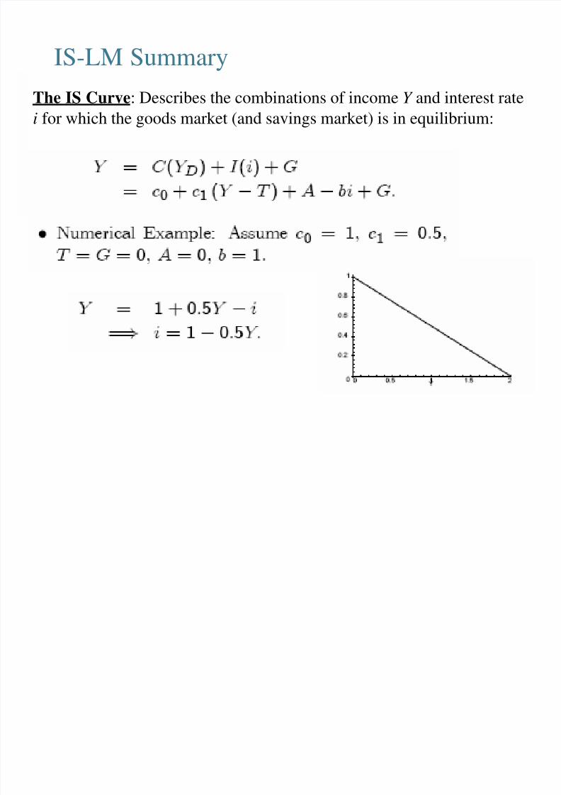
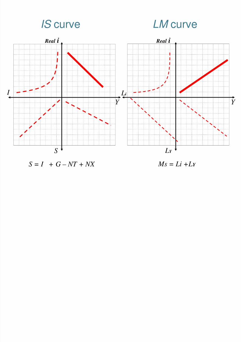
The IS Curve : Describes the combinations of income Y and interest ratei for which the goods market (and savings market) is in equilibrium:

IS-LM Summary



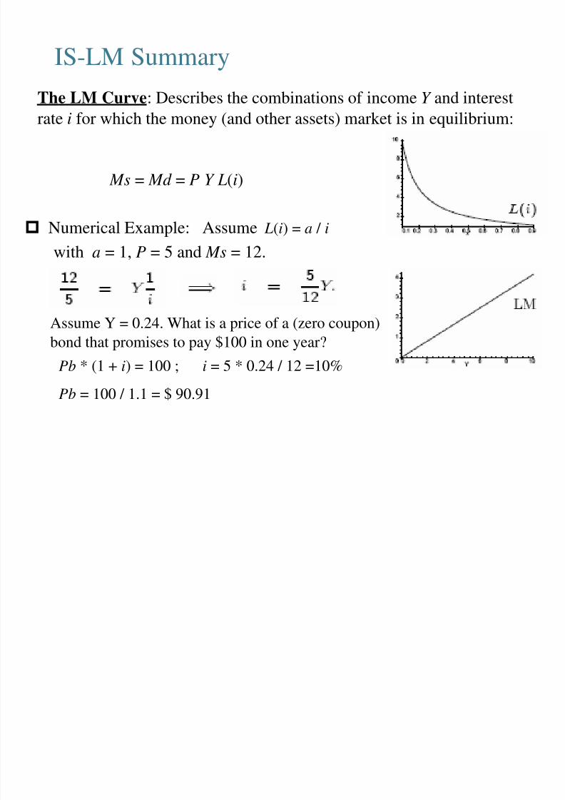
Assume Y = 0.24. What is a price of a (zero coupon)bond that promises to pay $100 in one year?

Numerical Example: Assume L(i) = a / iwith a = 1, P = 5 and Ms = 12.

The LM Curve : Describes the combinations of income Y and interestrate i for which the money (and other assets) market is in equilibrium:

Ms = Md = P Y L(i)

IS-LM Summary

Pb * (1 + i) = 100 ; i = 5 * 0.24 / 12 =10%

Pb = 100 / 1.1 = $ 90.91



IS curve

S

I

Real i

Y

LY

Li

Real i

Y

LM curve

S = I + G – NT + NX Ms = Li +L Y



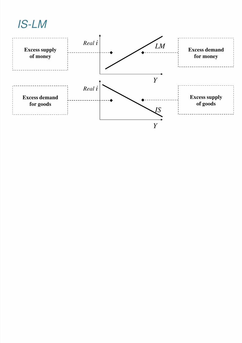
IS-LM

Y

Real i LM

Y

Real i

ISExcess demand

for goods

Excess supplyof money

Excess supplyof goods

Excess demandfor money



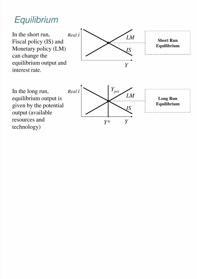
Equilibrium

Y

Real i LM

IS

Y

Real i Y pot

Y*

Long RunEquilibrium

Short RunEquilibrium

LM

IS

In the short run,Fiscal policy (IS) andMonetary policy (LM)can change theequilibrium output andinterest rate.

In the long run,equilibrium output is

given by the potentialoutput (availableresources andtechnology)



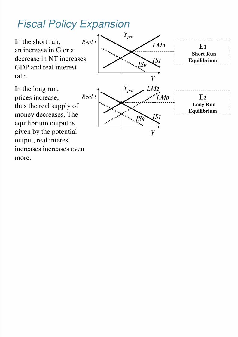
Fiscal Policy Expansion

Y

Real i LM 0

IS1

Y

Real i

E 1Short Run

Equilibrium

LM 0

IS1

In the short run,an increase in G or adecrease in NT increasesGDP and real interestrate.

In the long run,prices increase,thus the real supply of money decreases. Theequilibrium output isgiven by the potentialoutput, real interestincreases increases even

more.

IS0

IS0

LM 2

E 2Long Run

Equilibrium

Y pot

Y pot



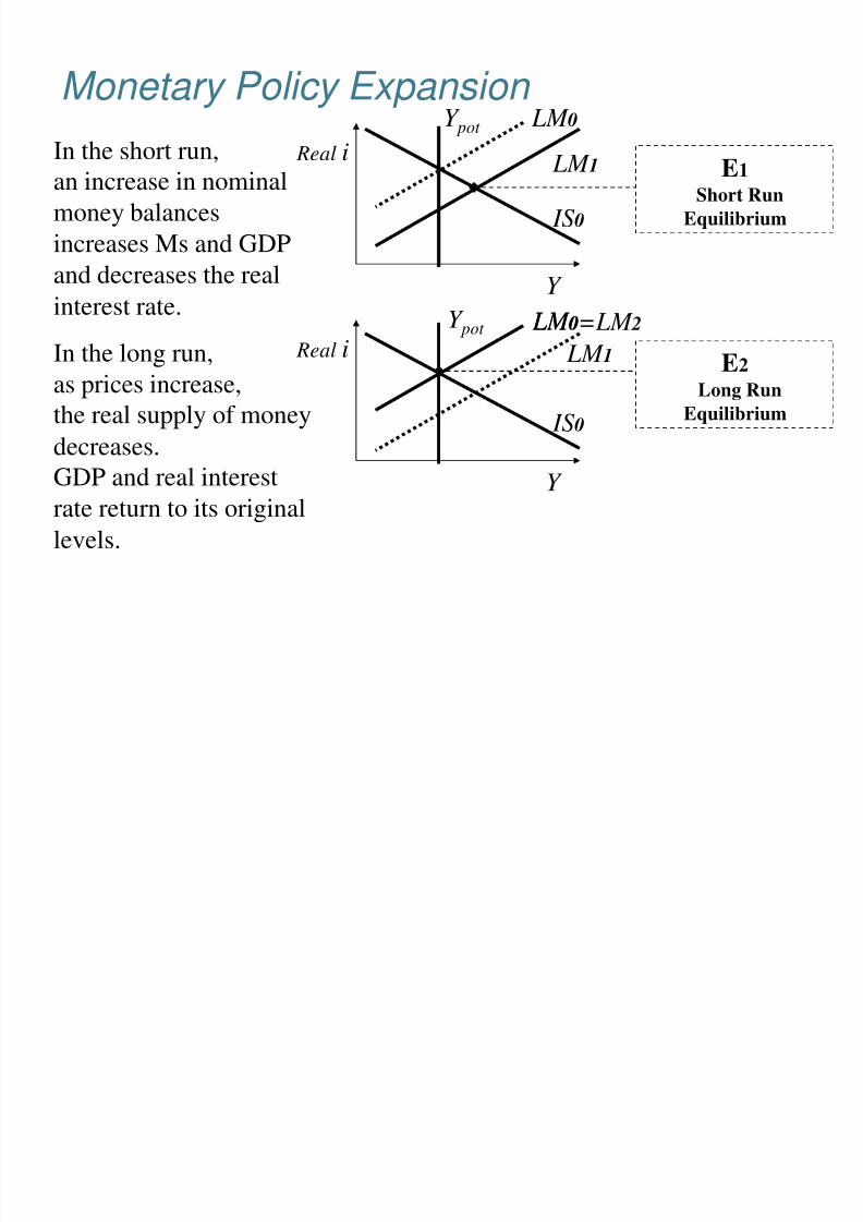
Monetary Policy Expansion

Y

Real i LM 1

IS0

Y

Real i

E 1Short Run

Equilibrium

LM 1

IS0

In the short run,an increase in nominalmoney balancesincreases Ms and GDPand decreases the realinterest rate.

In the long run,as prices increase,the real supply of moneydecreases.GDP and real interestrate return to its originallevels.

LM 0

E 2Long Run

Equilibrium

LM 0Y pot

Y pot LM 0 =LM 2



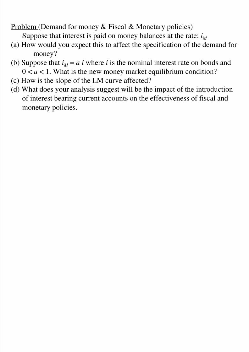
Problem (Demand for money & Fiscal & Monetary policies)Suppose that interest is paid on money balances at the rate: i M

(a) How would you expect this to affect the specification of the demand formoney?

(b) Suppose that i M

= a i where i is the nominal interest rate on bonds and0 < a < 1. What is the new money market equilibrium condition?

(c) How is the slope of the LM curve affected?(d) What does your analysis suggest will be the impact of the introduction

of interest bearing current accounts on the effectiveness of fiscal andmonetary policies.



Problem (Demand for money & Fiscal & Monetary policies)Suppose that interest is paid on money balances at the rate: i M

(a) How would you expect this to affect the specification of the demand formoney?

(b) Suppose that i M

= ai where i is the nominal interest rate on bonds and0 < a < 1. What is the new money market equilibrium condition?

(c) How is the slope of the LM curve affected?(d) What does your analysis suggest will be the impact of the introduction

of interest bearing current accounts on the effectiveness of fiscal andmonetary policies.

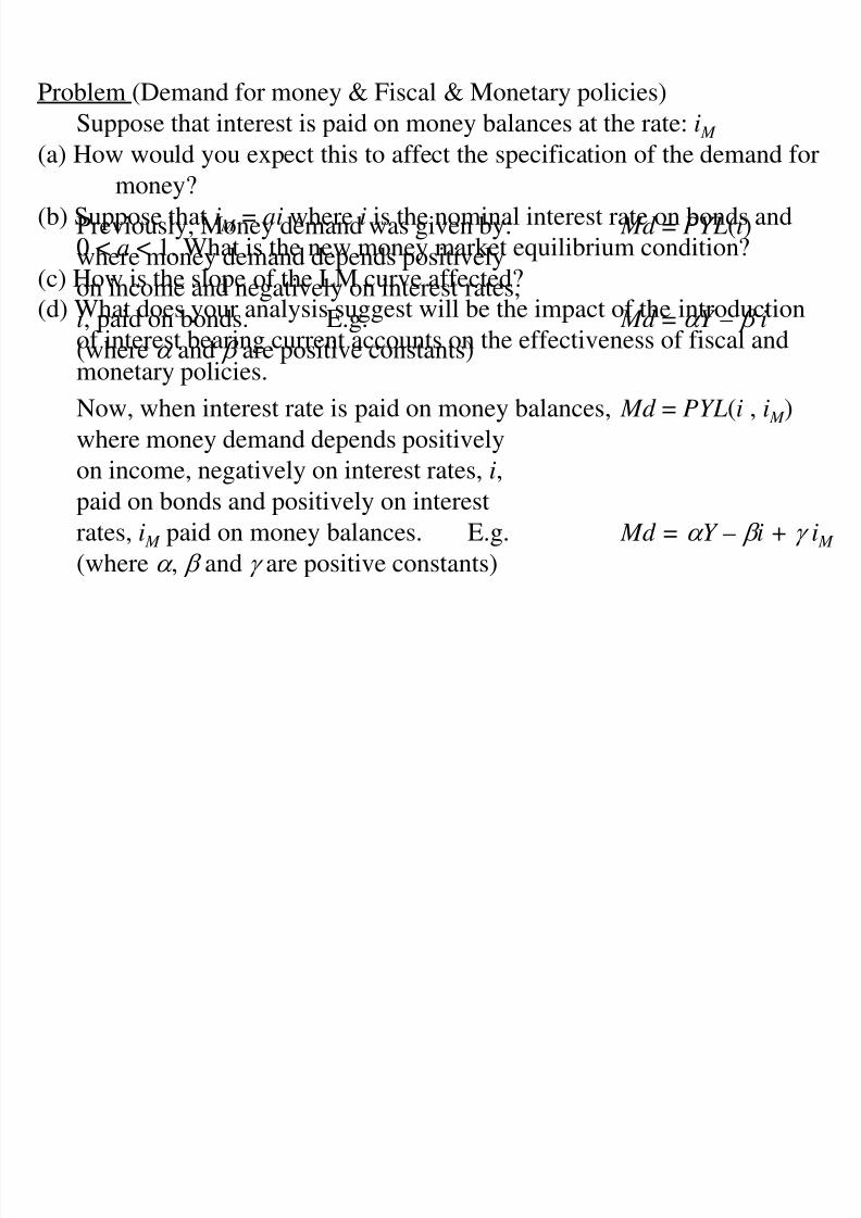
Previously, Money demand was given by: Md = PYL(i)where money demand depends positivelyon income and negatively on interest rates,i, paid on bonds. E.g. Md = α Y – β i

(where α and β are positive constants)

Now, when interest rate is paid on money balances, Md = PYL(i , i M )where money demand depends positivelyon income, negatively on interest rates, i,paid on bonds and positively on interestrates, i M paid on money balances. E.g. Md = α Y – β i + γ i M

(where α , β and γ are positive constants)



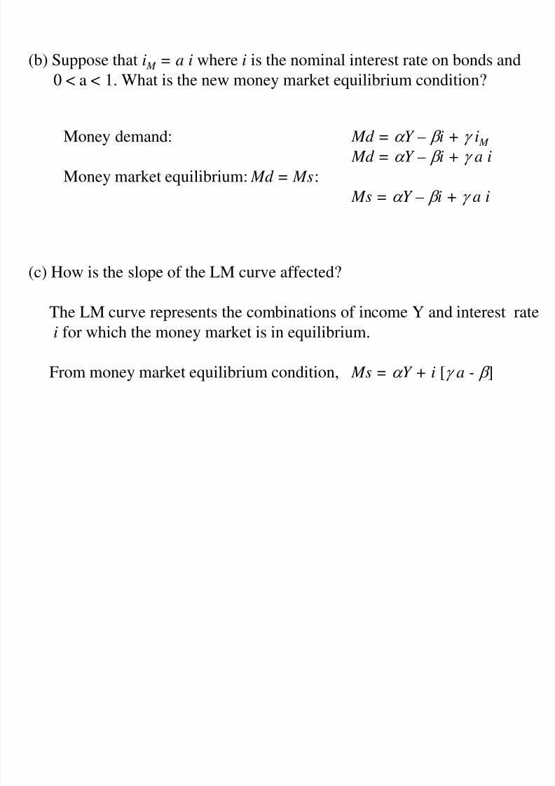
(b) Suppose that i M = a i where i is the nominal interest rate on bonds and0 < a < 1. What is the new money market equilibrium condition?

Money demand: Md = α Y – β i + γ i M

Md = α Y – β i + γ a iMoney market equilibrium: Md = Ms :

Ms = α Y – β i + γ a i

(c) How is the slope of the LM curve affected?

The LM curve represents the combinations of income Y and interest ratei for which the money market is in equilibrium.

From money market equilibrium condition, Ms = α Y + i [γ a - β ]



β α

aγ β α −

aγ β >

aγ <

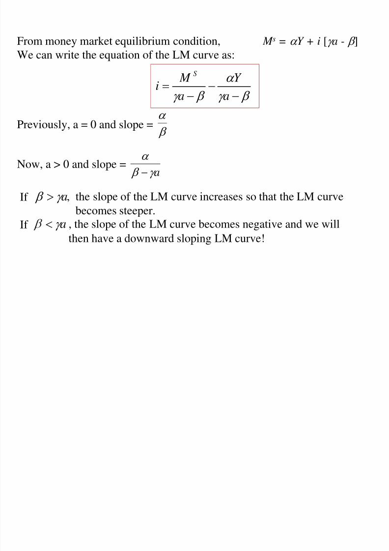
From money market equilibrium condition, M s = α Y + i [γ a - β ]We can write the equation of the LM curve as:

Previously, a = 0 and slope =

Now, a > 0 and slope =

If , the slope of the LM curve increases so that the LM curve

becomes steeper.If , the slope of the LM curve becomes negative and we will

then have a downward sloping LM curve!

β γ α

β γ −−

−=

aY

a M

iS



aγ >

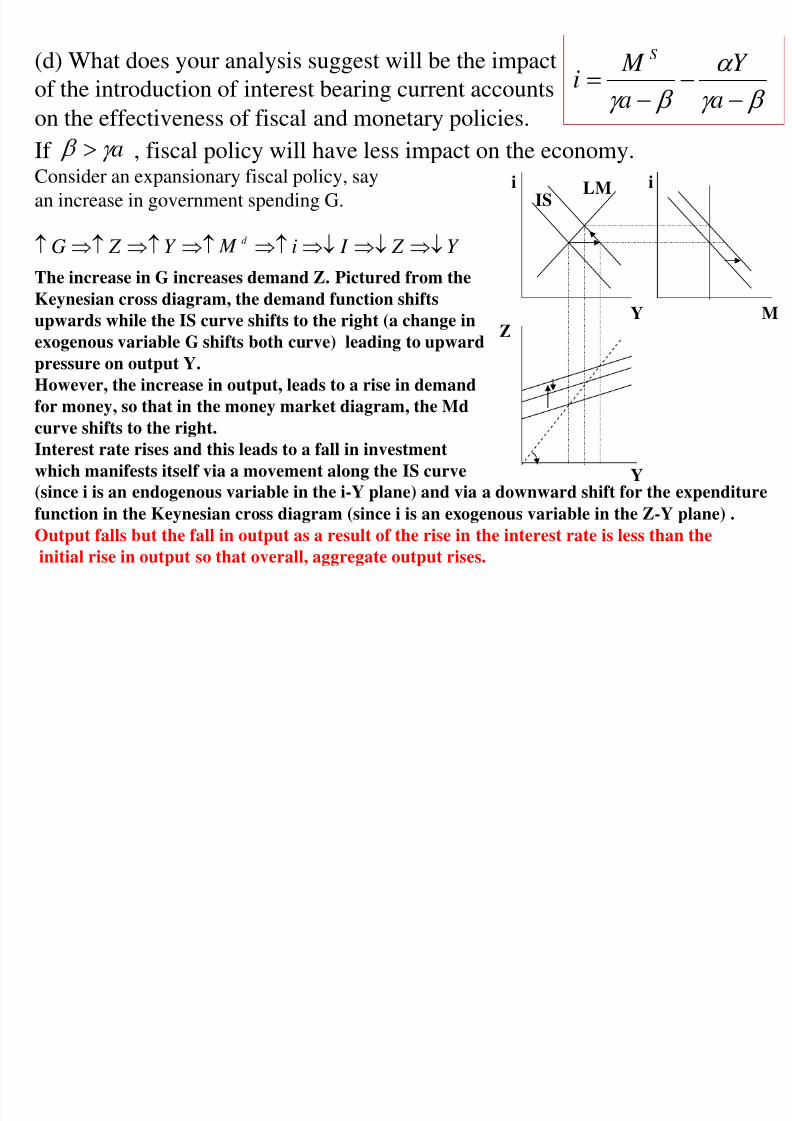
Y Z I iY Z G d ⇒↓⇒↓⇒↓⇒↑⇒↑⇒↑⇒↑↑

(d) What does your analysis suggest will be the impactof the introduction of interest bearing current accountson the effectiveness of fiscal and monetary policies.If , fiscal policy will have less impact on the economy.Consider an expansionary fiscal policy, sayan increase in government spending G.

The increase in G increases demand Z. Pictured from theKeynesian cross diagram, the demand function shifts

upwards while the IS curve shifts to the right (a change inexogenous variable G shifts both curve) leading to upwardpressure on output Y.However, the increase in output, leads to a rise in demandfor money, so that in the money market diagram, the Md

curve shifts to the right.Interest rate rises and this leads to a fall in investmentwhich manifests itself via a movement along the IS curve(since i is an endogenous variable in the i-Y plane) and via a downward shift for the expenditurefunction in the Keynesian cross diagram (since i is an exogenous variable in the Z-Y plane) .

Output falls but the fall in output as a result of the rise in the interest rate is less than theinitial rise in output so that overall, aggregate output rises.

ISLM ii

Y

Y

MZ

β γ

α

β γ −

−

−

=

a

Y

a

M i

S



aγ >

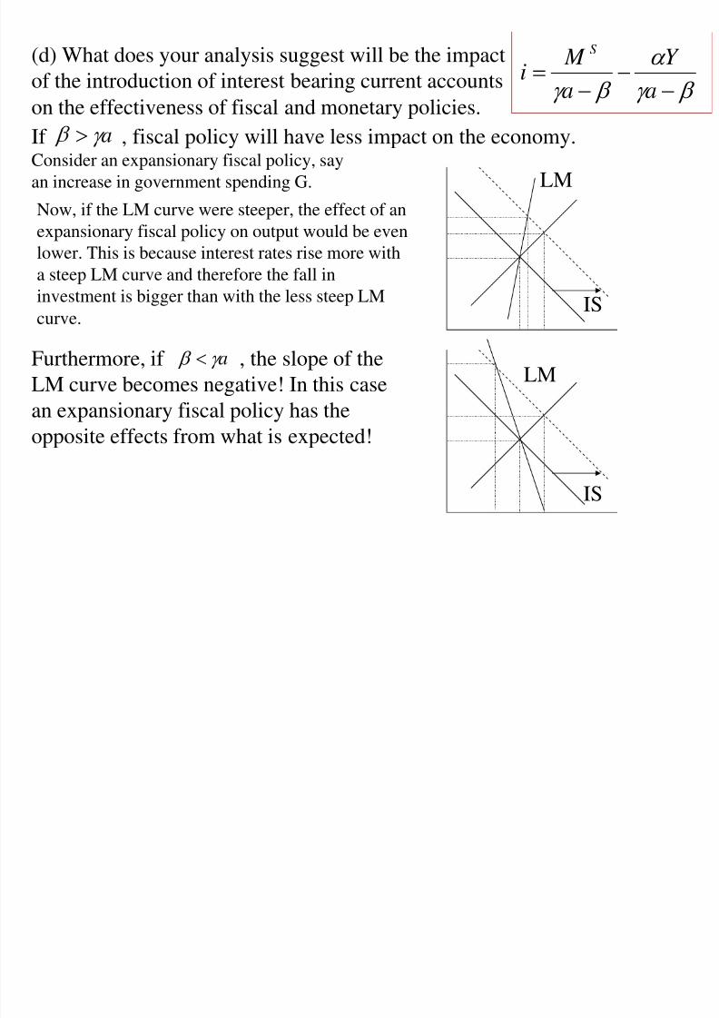
(d) What does your analysis suggest will be the impactof the introduction of interest bearing current accountson the effectiveness of fiscal and monetary policies.If , fiscal policy will have less impact on the economy.Consider an expansionary fiscal policy, sayan increase in government spending G.

Now, if the LM curve were steeper, the effect of anexpansionary fiscal policy on output would be evenlower. This is because interest rates rise more witha steep LM curve and therefore the fall ininvestment is bigger than with the less steep LMcurve.

aγ β <Furthermore, if , the slope of the

LM curve becomes negative! In this casean expansionary fiscal policy has theopposite effects from what is expected!

IS

LM

IS

LM

β γ

α

β γ −

−

−

=

a

Y

a

M i

S



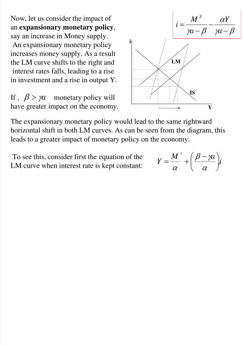
Now, let us consider the impact of an expansionary monetary policy ,say an increase in Money supply.An expansionary monetary policy

increases money supply. As a resultthe LM curve shifts to the right andinterest rates falls, leading to a rise

in investment and a rise in output Y.

If , monetary policy willhave greater impact on the economy.aγ β >

LM

IS

Y

i

The expansionary monetary policy would lead to the same rightward

horizontal shift in both LM curves. As can be seen from the diagram, thisleads to a greater impact of monetary policy on the economy.

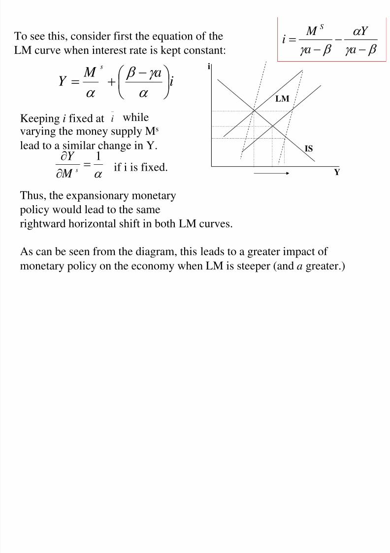
To see this, consider first the equation of the

LM curve when interest rate is kept constant:

β γ

α

β γ −

−

−

=

a

Y

a

M i

S

i

a M

Y

s

⎟

⎞⎜⎝ ⎛ −+=

α

γ β

α



ia M

Y s

⎟ ⎠ ⎞

⎜⎝ ⎛ −+=

α γ β

α

β γ

α

β γ −

−−

=

a

Y

a

M i

S

To see this, consider first the equation of the

LM curve when interest rate is kept constant:

−

i

α 1=∂∂ sY

Keeping i fixed at whilevarying the money supply M s

lead to a similar change in Y.

if i is fixed.

Thus, the expansionary monetary

policy would lead to the samerightward horizontal shift in both LM curves.

As can be seen from the diagram, this leads to a greater impact of

monetary policy on the economy when LM is steeper (and a greater.)

LM

IS

Y

i



β γ

α

β γ −

−−

=

a

Y

a

M i

S

LM

IS

Y

i

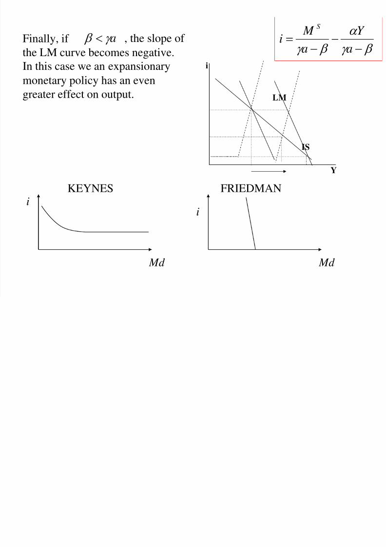
Finally, if aγ β < , the slope of

the LM curve becomes negative.In this case we an expansionarymonetary policy has an evengreater effect on output.

KEYNES FRIEDMAN

Md

i

Md

i

Documents

Is LM Summary