Is minimum-variance investing really worth the while?

An analysis with robust performance inference

Patrick Behr∗ Andre Guttler† Felix Miebs‡.

October 31, 2008

∗Department of Finance, Goethe-University Frankfurt, Mertonstr. 17, 60054 Frankfurt, Germany,E-mail: behr@finance.uni-frankfurt.de.†HCI Endowed Chair of Financial Services, Department of Finance, Accounting and Real Estate,

European Business School, International University, Rheingaustr. 1, 65375 Oestrich-Winkel, Germany,E-mail: andre.guettler@ebs.edu(Corresponding author).‡HCI Endowed Chair of Financial Services, Department of Finance, Accounting and Real Estate,

European Business School, International University, Rheingaustr. 1, 65375 Oestrich-Winkel, Germany,E-mail: felix.miebs@ebs.edu

Is minimum-variance investing really worth the while?

An analysis with robust performance inference

Abstract

This paper examines the risk-adjusted performance of the minimum-variance

equity investment strategy in the U.S. While earlier studies only relied on empirical

Sharpe ratio comparisons between the (constrained) minimum-variance strategy

and different benchmark portfolios, we employ bootstrap methods for statistical

inference concerning the Sharpe ratio, the Sortino ratio, certainty equivalents and

alpha measures based on several factor models. We confirm and provide robust

inference concerning earlier findings that constrained minimum-variance portfolios

do outperform a value weighted benchmark. Moreover, our findings are in line

with prior research, stating that minimum-variance portfolios do not outperform a

naively diversified benchmark in terms of the Sharpe ratio. Both our results are

invariant to the portfolio revision frequency and may be observed in all subperiods.

Nevertheless, we show the high sensitivity of the constrained minimum-variance

portfolios to the revision frequency and the imposed maximum portfolio weight

constraints.

1 Introduction

The foundations of modern portfolio theory go back to the seminal work of Markowitz

(1952; 1959). In his framework, portfolio selection is postulated as a trade-off between

risk and return, where efficient portfolios deliver a maximum return for a given level

of risk or, vice versa, deliver a minimum of risk for a given level of return. Ever since

then a vast amount of literature has been devoted to research about modern portfolio

selection. A considerable amount of this research has focused on the evaluation of the

out-of-sample performance of two portfolios on the efficient frontier, which comprises all

efficient portfolios, namely the tangency and the minimum-variance portfolio.

The tangency portfolio, as the portfolio with the largest excess return per unit of risk,

attracted researchers’ attention due to its theoretical foundation as the optimal portfolio

for an investor. Following Tobin’s mutual fund separation (1958), every investor should

hold (dependent on her risk aversion) a certain fraction of wealth in the tangency portfolio,

but should not alter the weight of any asset in the tangency portfolio.

Stein (1956), Frost and Savarino (1986), Jorion (1986) and Black and Litterman (1992),

amongst others, point out that the estimation of expected returns (from sample data),

which is necessary for the calculation of the tangency portfolio, is error prone and may

yield misleading results. Additionally, Goyal and Welch (2003a; 2007) and Butler et

al. (2001) show that even more advanced techniques for the return prediction, based on

predictive regressions, have a similarly poor out-of-sample performance. In line with this,

Bloomfield et al. (1977), Jobson and Korkie (1981a) and Jagannathan and Ma (2003)

find that the tangency portfolio does not outperform an equally weighted portfolio.

These sobering results concerning the performance of the tangency portfolio drew atten-

tion to the minimum-variance portfolio, the only portfolio on the efficient frontier that

requires the variance-covariance matrix as input parameter for the optimization. Merton

(1980), Jorion (1985), and Nelson (1992) point out that variance-covariance estimates

are relatively stable over time and can, hence, be predicted more reliably than returns.

Underpinning these results of lower estimation errors for the minimum-variance portfolio,

Baker and Haugen (1991) and Clarke et al. (2006) find an out-of-sample outperformance

of the minimum-variance portfolio relatively to a value weighted portfolio. Additionally,

Chan et al. (1999), Jagannathan and Ma (2003) and DeMiguel et al. (2007) point out that

the short-sale constrained minimum-variance portfolio outperforms the tangency portfolio

1

approach.

Evidence regarding a possible outperformance of the minimum-variance portfolio relative

to an equally weighted portfolio is less clear. Based on purely descriptive results, Chan et

al. (1999) and Jagannathan and Ma (2003) report higher out-of-sample Sharpe ratios for

the constrained minimum-variance portfolio (CMVP). Given their lack of statistical in-

ference, a robust conclusion whether the (constrained) minimum-variance strategy offers

superior risk-adjusted returns cannot be made. Employing a parametric test, DeMiguel

et al. (2007) find statistically indistinguishable differences in Sharpe ratios between the

minimum-variance portfolio and a value weighted and equally weighted portfolio. Given

this mixed evidence, the question whether minimum-variance investing is worthwhile ap-

pears to be rather unacknowledged so far.

The aim of this paper is to assess the risk-adjusted performance of the minimum-variance

strategy for equity investors using robust performance inference. Though the research

question, whether minimum-variance investing can deliver a risk adjusted outperformance

relatively to a value or equally weighted benchmark strategy, has already bween investi-

gated, we offer several new results and perspectives.

First, all aforementioned papers failed to provide robust evidence whether the minimum-

variance strategy is worthwhile to conduct. This paper is, to the best of our knowledge, the

first to use nonparametric performance tests between the minimum-variance investment

strategy employed and a naively diversified as well as a value weighted benchmark portfo-

lio. The employed nonparametric bootstrap approach should be better suited for this kind

of performance comparison since neither the strong assumption of normally distributed

nor independent and identically distributed (i.i.d.) returns are required.1 Furthermore,

we provide beside the Sharpe ratio performance comparisons for the Sortino ratio, alpha

measures based on diverse factor models and certainty equivalents in order to provide

robust evidence of possible performance differences.

Second, we are the first to base the derived results on the whole U.S. equity universe as

captured by the Center for Research in Security Prices (CRSP) stock database2, which

allows a comprehensive assessment of the considered research question. Contrary, all

1Evidence for non-normality of stock returns goes back to Fama (1965). Additionally, DeMiguel et al.(2007) note that ”this assumption is typically violated in the data”. Ledoit and Wolf (2008) shows thatthe commonly used parametric Sharpe ratio test by Jobson and Korkie (1981a) requires, likewise thecorrected version of the test by Memmel (2003), identical and independently distributed returns.

2For a closer description of the dataset see section 3.

2

aforementioned papers base their findings on either randomly drawn samples from the

CRSP database (e.g. Chan 1999 and Jagannathan and Ma 2003), stock index constituents

(e.g. Baker and Haugen 1991 and Clarke et al. 2006) or sector portfolios (DeMiguel et

al. 2007).

During the course of our paper, we reproduce with our dataset a part of the work by

DeMiguel et al. (2007) - in particular by using a maximum portfolio weight3 of 2% in the

portfolio optimization process. Despite striking differences in the inference methodology4

and different datasets, we find evidence in line with DeMiguel et al. (2007) that the 2%

CMVP offers no outperformance compared to naively diversified portfolios. Thus, in this

setup, we do not corroborate (descriptive) findings by Chan et al. (1999) and Jagannathan

and Ma (2003). Nevertheless, we do find evidence, by relaxing the maximum portfolio

weight constraint, that CMVPs deliver a favorable performance in terms of alpha based on

every considered factor model in comparison to the equally weighted benchmark portfolio.

Performance comparisons relative to the value weighted benchmark portfolio broadly show

that the CMVPs outperform the value weighted benchmark portfolio.

The remainder of the paper is organized as follows: section two reviews the methodology

and gives a thorough outline of the employed nonparametric performance tests. Section

three describes the data used. Section four reports and discusses the empirical results

whereas section five presents robustness checks. Finally, the last section concludes the

findings of this paper.

2 Methodology

This section is divided into three parts. First, we describe the portfolio optimization

methodology used for the derivation of the CMVPs. This is followed by a short review of

the various performance measures, while the third part of this section provides a thorough

outline of the employed nonparametric bootstraps for the statistical inference concerning

the comparison of the considered portfolio performance metrics.

3In the following we use the terms ”maximum portfolio weight”, ”upper bound” and ”upper constraint”synonymously.

4DeMiguel et al. (2007) use the Jobson and Korkie (1981a) parametric Sharpe ratio test in its correctedversion by Memmel (2003), while we employ a nonparametric bootstrap for inference concerning theequality of Sharpe ratios of the minimum-variance portfolio and the respective benchmarks.

3

2.1 Portfolio optimization

Despite the fact that estimates of the variance-covariance matrix are less error prone than

those of expected returns, the estimation error problem is far from alleviation. Actually,

Chan et al. (1999) point out that the estimation error in variance-covariance estimates

from sample data is still substantial. For example, they find a correlation of only 34%

(18%) between the in-sample variance-covariance matrix and the out-of-sample covariance

matrix, based on a 36 (12) months realization period.

There are various ways to deal with estimation errors in order to improve the out-of-

sample reliability of parameter estimates. In general, three major approaches can be

distinguished: factor model approaches, Bayes-Stein shrinkage estimators and the imple-

mentation of portfolio weight constraints.5

Starting with the postulation of Sharpe’s (1963; 1964) one factor model, the use of fac-

tor models, not only to explain and predict returns, but also to estimate the variance-

covariance matrix by imposing the factor model structure on the estimator of the variance-

covariance matrix, became popular. The basic assumption underlying the one factor

model in the context of covariance prediction is that the mutual return correlations be-

tween all assets is attributable to a common factor - the market index. Chan et al. (1999)

provide a comprehensive examination of various factor models and their capability of

out-of-sample variance-covariance prediction. They show, however, that the forecasted

variance-covariance matrix based on historical returns performs for the purpose of port-

folio optimization about as well as factor model estimates.

The most prominent approach in dealing with the estimation error problem is probably

the Bayes-Stein shrinkage estimator. Initially proposed by Stein (1956) and James and

Stein (1961), Bayes-Stein shrinkage estimators have widely been applied to the estimation

of both input parameters of portfolio optimization, expected returns6 and the variance-

covariance matrix7. However, Jobson and Korkie (1980) show that shrinkage estimators

do not perform well in small samples. Additionally, Jagannathan and Ma (2003) reveal

that the Bayes-Stein improvements in the variance-covariance matrix are minor relative

5Other solutions include equilibrium constraints (Black and Litterman 1992), optimal combinations ofportfolios (Garlappi et al. 2007) and the formulation of robust portfolio optimization problems, whichdirectly incorporate a measure of the parameter uncertainty into the optimization procedure. Fabozziet al. (2007) provide a sound survey of the latter approach.

6See for instance Jobson et al. (1979), Jobson and Korkie (1981a) and Jorion (1985; 1986)7We refer to Ledoit and Wolf (2003) for an application of shrinkage techniques to the variance-covariancematrix.

4

to estimates based on historical data. While DeMiguel et al. (2007) confirm this finding

for both, the variance-covariance matrix and expected returns.

The implementation of portfolio weight constraints in order to avoid highly concentrated

portfolios and extreme portfolio positions, that are frequently derived in the mean-variance

optimization procedure8, has, to the best of our knowledge, first been applied by Frost and

Savarino (1988). Nevertheless, Jagannathan and Ma (2003) were the first who studied the

shrinkage like effect of upper and lower (short-sale constraint) bounds on portfolio weights,

preventing large exposure to single assets. Despite their promising findings only little

attention has been payed to the proposed adjustments since then. However, DeMiguel

et al. (2007) recently showed that the minimum-variance portfolio with the proposed

portfolio weight restrictions delivers the most favorable out-of-sample performance in

terms of the Sharpe ratio.

In line with DeMiguel et al. (2007) and Chan et al. (1999) we adopt the constrained

myopic minimum-variance portfolio setup proposed by Jagannathan and Ma (2003) that

builds on the Markowitz (1952) portfolio selection framework. Since the crucial assump-

tion of normally distributed returns is typically violated in the data.9 we meet the as-

sumption that the investor’s utility function is quadratic in order to keep the portfolio

optimization approach valid.10 Thus, we employ the CMVP optimization setup on a

”rolling-sample” basis. Since the choice of sample size for the parameter estimation rep-

resents a delicate trade-off between an increase of statistical confidence and the incorpo-

ration of possibly irrelevant data11, we stick to the sample size choice of Chan (1999) and

Jagannathan and Ma (2003). Accordingly, the portfolio is rebalanced every three months

in the base case, taking the return observations of the last 60 months as input parameter

for the variance-covariance matrix estimation.12

Hence, we solve the standard myopic portfolio optimization problem, imposing the rec-

ommended constraints by Jagannathan and Ma (2003) in order to reduce the estimation

error and to achieve a shrinkage-like effect.13 Accordingly, we set on the portfolio weights

8See Green and Hollifield (1992), Chopra (1993) and Chopra and Ziemba (1993) for evidence concerningthis point.

9For evidence concerning this point see Fama (1965) and DeMiguel et al. (2007)10All portfolio optimization approaches that base on Markowitz (1952) require either normally distributed

returns or quadratic utility functions of investors.11See for this Jobson (1981b) and Levine (1972).12Additionally, we vary the portfolio revision frequency for robustness check purposes from three months

to six and twelve months. Results for this are reported in section 5.13Even though the setup is multi-period in nature, Mossin (1969), Fama (1970), Hakansson (1970; 1974)

and Merton (1990) show that ”under several sets of reasonable assumptions, the multi-period problem

5

a no-short sales constraint, wi,t ≥ 0 and an upper bound wmax, which is varied in one

percent steps in the range {wmax = 2%, 3%, ..., 20%}, on the weight a single stock may

have in the portfolio. After the optimization process the portfolio weights remain three

months14 unchanged up to the next optimization. Formally, this results in an optimization

problem for each period t of the following form15:

minwt w

′

tSwt s.t. (1)N∑i=1

wi,t = 1 (2)

wi,t ≥ 0, for i = 1, 2, ..., N (3)

wi,t ≤ wmax, for i = 1, 2, ..., N (4)

The Kuhn-Tucker conditions (necessary and sufficient) are accordingly:

∑j

Si,jwj − λi + δi = λ0 ≥ 0, for i = 1, 2, ..., N (5)

λi ≥ 0 and λi = 0 if wi > 0, for i = 1, 2, ..., N (6)

δi ≥ 0 and δi = 0 if wi < wmax, for i = 1, 2, ..., N (7)

The notation hereby is as follows: w denotes the vector of portfolio weights, S the empir-

ically estimated variance-covariance matrix, λ the vector of Lagrange multipliers in the

non negativity constraint of portfolio weights, δ the multipliers of upper bound portfolio

weight constraints and λ0 the multiplier for the portfolio weights to sum up to one.

2.2 Performance metrics

In a second step we evaluate the out-of-sample performance of the CMVP and compare

it to both, a value weighted benchmark portfolio, which serves as a market proxy, and

an equally weighted portfolio, which is considered as a simple benchmark asset allocation

can be solved as a sequence of single-period problems” (Elton and Gruber 1997).14The portfolio revision frequency is varied for robustness check pruposes to six and twelve months.

Results for these revision frequencies are reported in section 5.2.15The notation and variable explanation follows closely Jagannathan (2003). Bold factors indicate vectors

and matrices, whereas e.g. wi denotes the i-th element of vector w.

6

strategy following for instance Bloomfield et al. (1977) and DeMiguel et al. (2007).16

In order to provide a broad picture of risk adjusted portfolio performance, we report

various performance measures which incorporate different conceptual measures of risk.

Accordingly, we provide evidence based on the certainty equivalent (CEQ)17, the Sharpe

(SH) and Sortino (SR) ratio as well as on alpha measures based on a one factor model (as

initially proposed by Jensen 1969), the Fama and French (1992) three factor and Carhart

(1997) four factor model, which are given by

SH =rp − rfσp

(8)

SR =rp − rfσdp

(9)

CEQ = rp −γ

2σ2p (10)

αp = rp,t −K∑k=1

βp,krk,t − εp,t, with ε ˜ Fp(0, σ2) (11)

Thereby denotes rp the return, σp the standard deviation and σdp the downside deviation18

of portfolio p, while αp stands for the portfolio specific constant, factor independent,

return,∑K

k=1 βp,k the sensitivities of the portfolio return relative to the return of the K

explanatory factors rk,t and εp,t the portfolio specific white noise error term.

2.3 Statistical performance metric inference

In order to check upon the statistical significance between the derived performance mea-

sures of the CMVPs and the considered benchmarks, we employ nonparametric bootstraps

for a robust performance measure inference. This is noteworthy since none of the earlier

mentioned papers employed a robust inference methodology for the comparison between

the (constrained) minimum-variance strategy and alternative investment strategies. An

exception is the work by DeMiguel et al. (2007), who employed a parametric Sharpe

16For convenience and following the common acceptance of the CRSP value and CRSP equally weightedmarket indices as market proxies (see Lehmann and Modest 1987) we opted to choose both as benchmarkportfolios.

17We assume that investors have quadratic utility functions which commonly accepted (see e.g. DeMiguelet al. 2007). We choose to set the risk aversion parameter to γ = 4 in order to assess the profitabilityof the CMVPs from the point of view of a highly risk averse investor

18For the purpose of our paper, we set the shortfall threshold to zero, in order to have a common, nonportfolio specific shortfall threshold for all portfolios in the analysis.

7

ratio test by Jobson and Korkie (1981b)19. Nevertheless, it is important to point out

that the parametric Sharpe ratio test by Jobson and Korkie (1981b) (as well as in its

corrected version by Memmel 2003) requires the strong assumption of normally and i.i.d.

distributed portfolio returns.20 The effect of non-normality of returns on this test and the

resulting inappropriateness is discussed by Ledoit and Wolf (2008).

We have therefore opted to use a nonparametric bootstrap approach, which was initially

proposed by Efron (1979). The superiority of the bootstrap approach vis-a-vis parametric

tests is twofold. First, it does not require any assumption about the distribution of the

considered performance measures nor their differences. Instead, our approach allows ous

to draw inference from our sample distribution. Second, Navidi (1989) showed that the

bootstrap is under all circumstances at least as good as the normal approximation which

is required for the widely used test by Jobson and Korkie (1981b). The use of bootstrap

methodology for robust performance metric inference has been highlighted by Morey and

Vinod (1999) and Kosowski et al. (2004; 2007) with regard to the Sharpe ratio, using a

simple observation bootstrap, and the factor model based alpha measures, using a residual

bootstrap respectively.

2.3.1 Observation bootstrap

Our approach towards testing for the equality of performance measures incorporating a

total measure of risk, namely the CEQ, the Sharpe and Sortino ratios follows the work by

Morey and Vinod (1999) and can be summarized as follows: From the empirical sample

comprising N monthly returns we draw a random return rp,t from the time series of

portfolio p with replacement. It is important to note that this is done pair wise in a

timely fashion, meaning that the return of the same randomly selected month is chosen

from the respective time series of the benchmark portfolio returns rbm,t. This is repeated n

times, leaving a bootstrap sample of n returns for each CMVP p {rp,t with t = 1, 2, ..., n}

and benchmark portfolio bm {rbm,t with t = 1, 2, ..., n}. Repeating the prior step B times

yields B bootstrap samples for every CMVP p {Sbp with b = 1, 2, ..., B} and benchmark

portfolio bm {Sbbm with b = 1, 2, ..., B}, each containing n returns. For each of the B

bootstrap samples we compute the Sharpe and Sortino ratio differences between each

19Memmel (2003) proposed a minor correction for this test statistic.20Evidence concerning the non-normal distribution of the CMVP returns (at least for our results) is

provided in the tables 3 and 8.

8

particular CMVP and the (naively or the value weighted) benchmark portfolios. Sorting

each of the resulting B CEQ, Sharpe and Sortino ratios differences in a vector enables us

to construct confidence intervals and to conduct hypothesis testing.

Point of interest is the confidence level at which the CMVP offers a statistically significant

outperformance relative to the considered benchmark portfolios. Accordingly, we compute

the p-values for the one sided hypotheses that the difference between a particular portfolio

performance measure of the CMVP and the benchmark portfolio (either equally or value

weighted) is smaller or equal to zero:

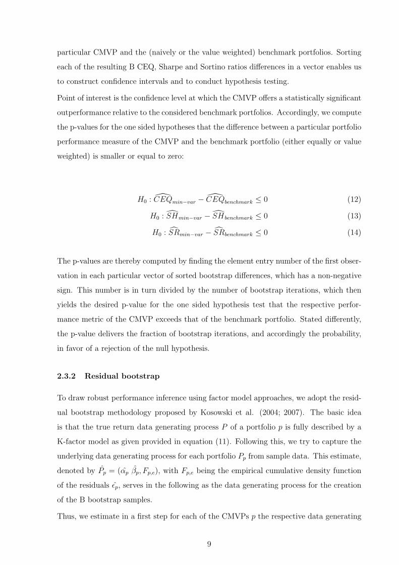
H0 : CEQmin−var − CEQbenchmark ≤ 0 (12)

H0 : SHmin−var − SHbenchmark ≤ 0 (13)

H0 : SRmin−var − SRbenchmark ≤ 0 (14)

The p-values are thereby computed by finding the element entry number of the first obser-

vation in each particular vector of sorted bootstrap differences, which has a non-negative

sign. This number is in turn divided by the number of bootstrap iterations, which then

yields the desired p-value for the one sided hypothesis test that the respective perfor-

mance metric of the CMVP exceeds that of the benchmark portfolio. Stated differently,

the p-value delivers the fraction of bootstrap iterations, and accordingly the probability,

in favor of a rejection of the null hypothesis.

2.3.2 Residual bootstrap

To draw robust performance inference using factor model approaches, we adopt the resid-

ual bootstrap methodology proposed by Kosowski et al. (2004; 2007). The basic idea

is that the true return data generating process P of a portfolio p is fully described by a

K-factor model as given provided in equation (11). Following this, we try to capture the

underlying data generating process for each portfolio Pp from sample data. This estimate,

denoted by Pp = (αp βp, Fp,e), with Fp,e being the empirical cumulative density function

of the residuals εp, serves in the following as the data generating process for the creation

of the B bootstrap samples.

Thus, we estimate in a first step for each of the CMVPs p the respective data generating

9

process, Pp, from the sample data. Following this, we store the estimated parameter

values of αp, βp, the t-value of αp, as well as the time series of the estimated residuals

εp,t with t=1,2,...,T.

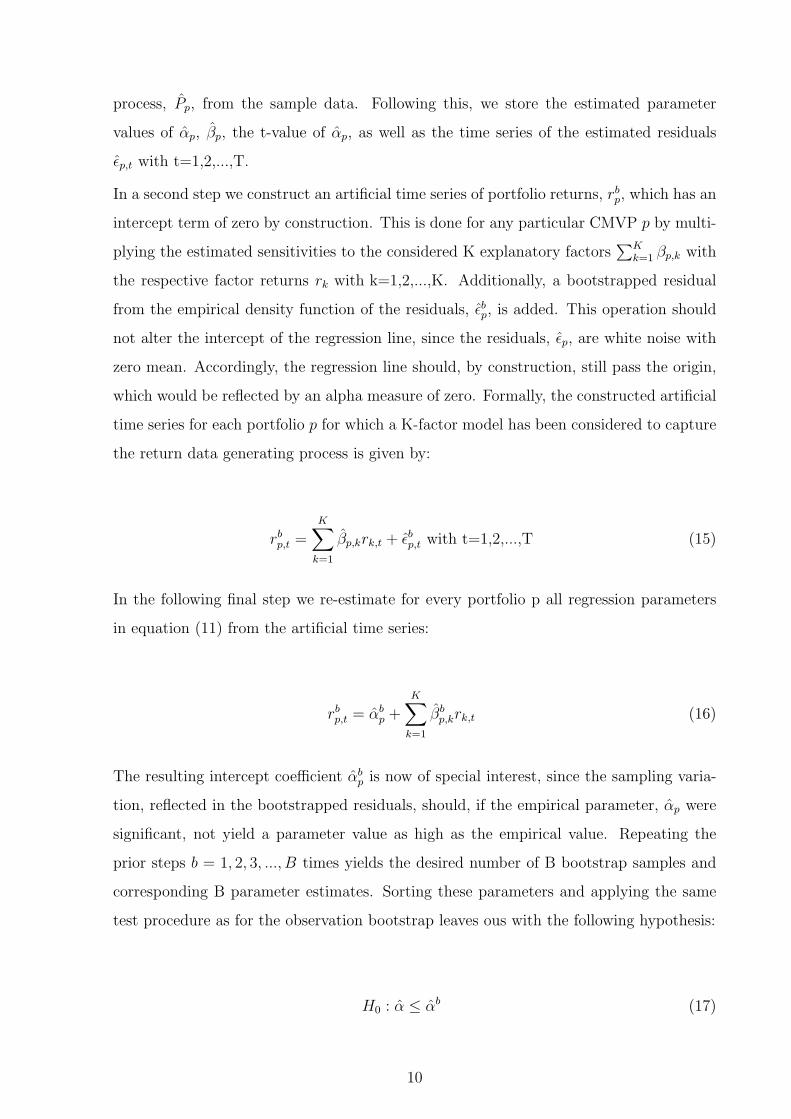
In a second step we construct an artificial time series of portfolio returns, rbp, which has an

intercept term of zero by construction. This is done for any particular CMVP p by multi-

plying the estimated sensitivities to the considered K explanatory factors∑K

k=1 βp,k with

the respective factor returns rk with k=1,2,...,K. Additionally, a bootstrapped residual

from the empirical density function of the residuals, εbp, is added. This operation should

not alter the intercept of the regression line, since the residuals, εp, are white noise with

zero mean. Accordingly, the regression line should, by construction, still pass the origin,

which would be reflected by an alpha measure of zero. Formally, the constructed artificial

time series for each portfolio p for which a K-factor model has been considered to capture

the return data generating process is given by:

rbp,t =K∑k=1

βp,krk,t + εbp,t with t=1,2,...,T (15)

In the following final step we re-estimate for every portfolio p all regression parameters

in equation (11) from the artificial time series:

rbp,t = αbp +K∑k=1

βbp,krk,t (16)

The resulting intercept coefficient αbp is now of special interest, since the sampling varia-

tion, reflected in the bootstrapped residuals, should, if the empirical parameter, αp were

significant, not yield a parameter value as high as the empirical value. Repeating the

prior steps b = 1, 2, 3, ..., B times yields the desired number of B bootstrap samples and

corresponding B parameter estimates. Sorting these parameters and applying the same

test procedure as for the observation bootstrap leaves ous with the following hypothesis:

H0 : α ≤ αb (17)

10

Since the t-value has more favorable statistical properties, due to the additional coverage

of the estimation precision of α, Kosowski et al. (2004; 2007) propose to bootstrap the

t-value.21 Following this argument, the resulting one sided hypothesis to test for is given

by:

H0 : tα ≤ tαb (18)

3 Data

Our dataset comprises the entire CRSP monthly stock database from April 1964 to De-

cember 2007. From this database, we only consider stocks in the optimization that have

non-zero returns and no missing values in the variance-covariance estimation period of 60

months prior to the optimization’s point in time. It is important to stress the necessity

of this filter since thin trading, reflected in limited or even no trading of stocks, drives

the covariance of these illiquid stocks with other stocks towards zero. In consequence of

the resulting downward biased covariance, foremost illiquid stocks will be selected so that

the performance will likely be driven by soaking up the stock market inherent liquidity

premium22. In order to avoid these thin trading effects, the aforementioned filter is em-

ployed.23 In case of missing values in the out-of-sample period we opted to set the stock

return to zero.

Finally, we follow the argument by Chan et al. (1999), who claim that the variance-

covariance matrix becomes too noisy if very small and micro capitalized firms are included

in the sample. Hence, we include in our final sample only those stocks that are in the

upper 80% size percentile (according to their market capitalization) and have a stock price

of more than $5.

Time series data for interest rates and factor return data for the factor models described

21We control for autocorrelation and heteroscedasticity using the autocorrelation and heteroscedasticityconsistent covariance matrix from Newey and West (1987).

22For evidence concerning the liquidity premium inherent in stock markets see Pastor and Stambaugh(2003).

23Despite the availability of adjustment procedures for the thin trading effect concerning the covarianceestimation (see e.g. Scholes and Williams 1977 and Dimson 1979), none of these adjustments has provento account properly for the thin trading effect. Evidence for this is provided by a comprehensive studyby McInish and Wood (1986).

11

in section 2.2 are obtained from Kenneth French’s website24, while the National Bureau

of Economic Research (NBER) recession period data, which we use for the determination

of U.S. recession periods25 is taken from the corresponding NBER website26.

4 Empirical results

The first part of this section describes the empirical performance measures of the CMVPs

with a portfolio revision frequency of three months over the complete sample period from

April 1968 to December 2007, while the second part provides statistical inference for the

empirical results and checks upon the significance of the empirical findings.

4.1 Descriptive performance metric analysis

Since the minimum-variance approach aims at the reduction of risk it is suggestive to

assess the empirical standard deviation of the CMVPs first. Quite obvious is the almost

nondecreasing pattern of standard deviations for the less CMVPs, which is accompanied

by a decreasing average number of stocks in the respective minimum-variance portfo-

lios. Accordingly, the observable increase in standard deviations can be attributed to

an increase in idiosyncratic risk, due to the reduced deterministic diversification of less

restrictively CMVPs. This effect is reflected in the declining values of the adjusted R2

as depicted in tables 1 and 2, which is observable for every considered benchmark port-

folio and factor model. Noteworthy is however the reduced standard deviation of the

CMVPs. As depicted in table 3 the CMVPs deliver, up to a portfolio weight constraint

of 8% (19%), standard deviations below those of the value (equally) weighted benchmark

portfolio. Nevertheless, this risk reduction bares the ”cost” of lower returns.27

A quantification of the observable trade-off between risk reduction and return is given

by the described performance metrics in section 2.2. The broad picture in table 3 shows

that all CMVPs clearly outperform the value weighted benchmark based on all perfor-

mance metrics that incorporate a total measure of risk. This is especially interesting for

24http://mba.tuck.dartmouth.edu/pages/faculty/ken.french/data_library.html25We are in line with other studies (e.g. Campbell et al. 2001 and Goyal and Santa-Clara 2003b) by

defining U.S. recession periods based on the NBER recession data.26http://www.nber.org/cycles/recessions.html27We would like to pronounce at this point that this trade-off is ex post in nature since the ”cost” of

lower returns has not been considered in the optimization objective, which only aims at the reductionof risk, irrespective of the associated return.

12

less CMVPs with a higher standard deviation than the value weighted benchmark port-

folio. It suggests that the higher return of the CMVPs overcompensates the increased

standard deviation. In line with this, all CMVPs performed worse in terms of the afore-

mentioned performance metrics compared to the equally weighted benchmark portfolio,

which achieved a higher return at a higher standard deviation than (almost) every CMVP.

A completely different impression arises if one considers the factor model based alpha

measures. Irrespective of the employed factor model and benchmark portfolio, all factor

models achieve a (in some cases substantially) positive alpha. Though this may be en-

couraging at first sight, it is important to highlight the associated regression statistics as

well as the behavior of the alpha measures with respect to the maximum portfolio weight

constraint.

Irrespective of the considered factor model, the alpha measure follows a hump shaped

pattern with respect to the maximum portfolio weight constraint, which is attributable

to the annualized mean return behaivor.28 Though this comovement may seem surprising

at first sight, the effect becomes clearer by taking the fairly constant absolute values of

systematic risk, as measured by the beta factors, into account. The increasing share of

non-systematic risk for less CMVPs, which is at least partially accompanied by increas-

ing returns (up to a maximum portfolio weight of 11%) casts nevertheless doubts upon

the postulation that systematic risk is the only source of risk which is rewarded at the

market.29

Concluding the empirical results, the CMVPs seem to outperform the value weighted

benchmark portfolio based on all considered performance metrics that incorporate a total

measure of risk. The opposite of this finding holds for the equally weighted benchmark

portfolio. If one assesses the performance based on the alpha measure, all CMVPs seem

to outperform both benchmark portfolios. Within the group of CMVPs, the empirical

trade-off between risk and return seems to be optimal for portfolios with a maximum

portfolio weight in the range between 8% - 11%.

28This is mirrored in a cross correlation of 0.934 (0.935) between the four factor alpha and the equally(value) weighted benchmark portfolio. The cross correlations between the other factor model basedalphas and the annualized mean returns are likewise well above 0.9.

29In the ongoing discussion whether idiosyncratic risk has explanatory power concerning the cross sectionof returns (and may thus be rewarded), Malkiel and Xu (1997; 2004) and Goyal and Santa-Clara (2003b)provide evidence in favor of the paper, while Bali et al. (2005) contradict those results.

13

4.2 Robust performance metric inference

Inference concerning the thus far derived empirical findings of the CMVP performance is

drawn by the bootstrap approaches described in section 2.3. Given the empirical evidence

of the non-normality of the CMVP returns, provided by the Jarque-Berra test p-values

in table 3, we stress once more the necessity of bootstrap inference. Accordingly any

inference for the Sharpe ratio based on the parametric Sharpe ratio test by Jobson and

Korkie (1981a) in its corrected version by Memmel (2003) would be incorrect - at least

for our data. We turn in the following to the CMVP performance inference relative to

the value weighted benchmark portfolio, which is followed by the assessment relative to

the equally weighted benchmark portfolio. Beside the bootstrap inference concerning

the performance metrics described in section 2.2, we provide inference for the annualized

mean return and standard deviation of the CMVPs. This is especially important for

the assessment whether the empirically observable overcompensation of risk by return,

reflected in the empirical performance metric pattern, is statistically significant.30

The bootstrapped p-values in table 4 show that a significantly higher return compared

to the value weighted benchmark portfolio, at the 5% (10%) significance level, has only

been delivered by the CMVPs with a maximum portfolio weight restriction of 9% - 11%

(6% - 14% and 20%). This proves that the empirical observation of higher returns for

every CMVP in comparison to the value weighted benchmark portfolio is statistically not

signficant for most portfolios. Broadly in line with the empirical evidence is the reduction

of the standard deviation. The standard deviations of the CMVP with a maximum port-

folio weigh constraint of 6% and less are accordingly significantly reduced in comparison

to the value weighted benchmark portfolio.

Most interestingly is the assessment whether the empirically observable domination of the

return over the risk effect is of statistical significance. Starting with the alpha measures31,

the empirically observable dominance of the return effect seems to be underpinned by the

bootstrap inference. All minimum-variance portfolios in the maximum portfolio weight

30The p-values for the differences in annualized mean returns and standard deviations are derived bythe in section 2.3.1 described observation bootstrap for the one sided hypotheses that the differencebetween the annualized mean return (standard deviation) of the CMVP and the benchmark portfolio(either equally or value weighted) is equal or less than zero:H0 = µmin−var − µbenchmark ≤ 0H0 = σmin−var − σbenchmark ≤ 0

31We base in the following all alpha measure descriptions and interpretations on the four factor modelbased alpha measure, since the four factor model yields the highest adjusted R2 for all CMVP.

14

constraint range between 7%-17% (9%-10%) as well as the 20% maximum portfolio weight

constraint minimum-variance portfolio yield significant alphas on the 5% (10%) confidence

level. Nevertheless, it is important to be aware of the particularities associated with the

alpha measure in the context of the minimum-variance portfolio performance mentioned

in section 4.1. Taking a closer look, it shows that almost only those portfolios with

a statistically significant increase in the annualized mean return achieved a significant

alpha. Following this, the significance of the alpha measure for portfolios that have a

significant increase in annualized mean return does not come at a surprise, since the

systematic risk measure does not mirror the steady increase in total risk.

Based on the empirical results, the empirical Sharpe ratio and CEQ point estimates of

every CMVP have been higher for every CMVP. Nevertheless, the bootstrap inference

shows that only those portfolios with a maximum portfolio weight constraint of less than

13% (8%) for the Sharpe ratio and 12% (8%) for the CEQ delivered significantly bet-

ter performance metrics on the 10% (5%) confidence level. Accordingly, the bootstrap

reveals that CMVPs with a significantly reduced standard deviation (in comparison to

the value weighted benchmark portfolio) deliver significantly higher risk adjusted perfor-

mance metrics than the benchmark portfolio. Following this, the empirically observable

domination of the return over the risk effect may not be considered to be statistically

significant. Additional evidence for this is provided by the Sortino ratio. All considered

minimum-variance portfolios with a maximum portfolio weight of less than 12% (14%) de-

liver significantly higher Sortino ratios relative to the value weighted benchmark portfolio

on a 5% (10%) confidence level.

The statistical inference of the CMVP performance in comparison to the equally weighted

benchmark portfolio reveals almost no surprising insights. The empirically lower perfor-

mance metrics of the CMVP in comparison to the equally weighted benchmark portfolio

are underpinned by the bootstrap results in table 4. Accordingly, the one sided hypothe-

sis that the CEQ, Sharpe and Sortino ratios of the equally weighted benchmark portfolio

exceed those of the CMVPs may not be rejected.

A somewhat different impression arises again from the alpha measures, which clearly

points at an outperformance of the CMVPs. The problem with the alpha measure based

on the equally weighted benchmark portfolio is however the same as already described.

Concluding these first results, the broad picture shows that deterministic diversification,

15

which is achieved by restrictive maximum portfolio weight constraints, does significantly

reduce the realized out-of-sample portfolio risk, as measured by the standard deviation.

Nevertheless, it is empirically observable that the imposed maximum portfolio weight

constraints lead for the least and most restrictively CMVPs to a decline in the annualized

mean return. This is in turn reflected in the empirically declining values of risk adjusted

portfolio performance metrics that incorporate a total measure of risk.

The bootstrap inference proves however, that this empirical finding is not significant

for the most restrictively CMVPs. Contrary, it turns out that those portfolios with

the highest deterministic diversification have the statistically most significant outperfor-

mance based on total risk incorporating performance metrics in comparison to the value

weighted benchmark portfolio. A somewhat contrarian picture is presented by the sys-

tematic risk adjusted alpha measure. Due to the fairly stable share of systematic risk

across all CMVPs, those portfolios with a high annualized mean return achieve a statisti-

cally significant alpha, irrespective of the considered market proxy (benchmark portfolio).

Accordingly one may constitute that certain CMVPs (roughly all minimum-variance port-

folios with a portfolio weight constraint of 7% or less) significantly outperform the value

weighted benchmark portfolio based on risk adjusted performance.

This observation may not be confirmed in comparison to the the equally weighted bench-

mark portfolio. Though the most restrictively CMVPs significantly reduce the standard

deviation in comparison to the equally weighted benchmark portfolio, none of the CMVPs

achieves higher empirical performance metrics. This empirical finding is clearly under-

pinned by the bootstrap results.

5 Robustness checks

In this section we provide evidence of the constrained minimum-variance investment strat-

egy performance in different market phases. Additionally, we check upon the sensitivity

of our results with respect to the portfolio revision frequency. The section is accordingly

divided into two parts, whereby we assess the performance of the constrained minimum-

variance strategy over three subperiods first. The subperiods comprise in particular U.S.

recession periods as well as high volatility and low volatility periods. This is followed

by an assessment of the variability of our results with respect to the portfolio revision

frequency, which is in the second part of this section varied from three to six and twelve

16

months respectively.

5.1 Subsamples

The assessment of subperiods shall foremost yield insights concerning the robustness of

the derived results for the complete sample period and reveal whether the constrained

minimum-variance performance over the complete sample period is driven by any specific

subperiod. Attention is specifically paid to the best performing CMVP in each subperiod

in order to draw conclusions concerning the constancy of the optimal32 portfolio weight

constraint. Our choice of subsample periods, namely U.S. recession periods as well as

high and low idiosyncratic volatility periods, bases on the work by Kosowski (2004) and

Campbell et al. (2001) respectively.

Empirically recession periods are characterized by increased volatility and low (negative)

annualized mean returns for the equally (value weighted) benchmark portfolio. Moreover,

Kosowski (2004) argues that investors care especially about portfolio performance in re-

cession periods due to the high marginal utility of wealth of investors over these periods.

Accordingly improvements in the (risk adjusted) performance relative to the equally and

value weighted benchmark portfolios seem to be particularly valuable for investors.

The segregation into high and low idiosyncratic volatility periods follows Campbell et

al. (2001) who find a deterministic trend in idiosyncratic firm level volatility we choose

to assess the CMVP performance in both volatility market states, with the low idiosyn-

cratic volatility subsample from April 1968 to December 1985 and the high idiosyncratic

volatility subsample from January 1986 to December 1997.33 Campbell et al. (2001)

note that the ”correlation among individual stock returns declined”, while idiosyncratic

risk increased over their sample period. Accordingly, possible sensitivities of the CMVP

performance to the development of idiosyncratic risk and return correlations are assessed

over these two subperiods.

Starting with the U.S. recession periods, the big picture shows clearly the profitability

of the constrained minimum-variance approach, resulting in overall higher performance

metrics in comparison to both benchmark portfolios. Empirical evidence concerning the

32Optimal has in this context to be understood in the sense of empirically best performing.33Campbell et al. (2001) define the complete low idiosyncratic volatility period from July 1962 to Decem-

ber 1985. Since our sample starts in April 1968, statements concerning the low idiosyncratic volatilityperiod are accordingly based on the period from April 1968 to December 1985.

17

negative CEQ reveals that more risk averse investors still shy, despite the empirically

favorable risk return profile of the CMVPs, investments in any of the portfolios during

recession periods. Despite the overall encouraging empirical results, only few CMVPs

deliver a statistically significant better portfolio performance relative to the benchmark

portfolios. In comparison to the value weighted benchmark portfolio only those CMVPs

with a significantly higher return than the benchmark portfolio achieved significantly

higher Sharpe and Sortino ratios.34 Accordingly all CMVPs with a maximum portfolio

weight constraint of 5% (9%) and less achieved a higher Sharpe and Sortino ratios than

the value weighted benchmark portfolio on a 5% (10%) significance level. The favorable

results for the more restrictively CMVP are underpined by the alpha measure. Significant

alphas are only generated by the CMVPs with a maximum portfolio weight constraint of

4% and less on a 10% confidence level. Similar results for the alpha measure are obtained

if one considers the equally weighted benchmark portfolio as market proxy. Contrary,

inference concerning the Sharpe and Sortino ratios reveals that the empirically observable

outperformance of the equally weighted benchmark portfolio by the CMVPs is in no case

statistically significant.

To sum up the findings of this first subperiod assessment, the more restrictively CMVPs

achieve significantly higher returns at a lower risk, which is finally reflected in signifi-

cantly higher performance metrics in comparison to the value weighted benchmark. In

comparison to the equally weighted benchmark portfolio, almost every CMVP achieved a

substantial risk reduction and an empirically higher annualized mean return. Neverthe-

less, this does not result in statistically higher performance metrics that base on a total

measure of risk. Opposed to that, the most restrictively CMVPs deliver a substantial and

significant alpha. All in all, the more restrictively CMVPs seem to perform reasonably

well during recession periods.

Turning to the high and low volatility periods35, as defined by Campbell et al. (2001),

the empirical characteristics may be confusing at first sight. Both benchmark portfolios

exhibit higher standard deviations in the low than in the high volatility period. This

effect is attributable to the development of the correlations among stocks. As pointed out

by Campbell et al. (2001), the average correlation among stocks declined over time. The

34We do not focus on the CEQ since risk averse investors would, according to the empirically negativeCEQ measure, not have valued any of the CMVPs.

35We stress once more that the segregation bases upon the firm level specific and not on the market levelvolatility.

18

diversification effect of both benchmark portfolios in the low volatility period, from April

1968 to December 1985, has correspondingly been low, resulting in the comparably high

standard deviation of both benchmark portfolios. Turning to the CMVP performance,

the value weighted benchmark portfolio delivered in the low volatility period higher per-

formance metrics that incorporate a total measure of risk as well as positive alphas in

comparison to the value weighted benchmark portfolio. This observation may only par-

tially be confirmed for the high volatility period, namely for the most restrictively CMVPs.

Compared with the equally weighted benchmark portfolio, none of the CMVPs deliver

higher performance metrics based on a total measure of risk in the low volatility period.

Nevertheless, all CMVPs achieve positive alphas, which holds as well for the high volatil-

ity period. Beside the positive alphas, the most restrictively CMVPs achieve additionally

Sharpe ratios in excess of the equally weighted benchmark portfolio, while almost every

CMVP exhibits higher Sortino ratios than the equally weighted benchmark portfolio.

The bootstrap results in tables 6 and 7 underpin the empirical findings for the high and

low volatility periods. The significantly higher returns of the CMVP in comparison to

the value weighted benchmark portfolio lead in turn to significantly higher CEQ, Sharpe

and Sortino ratios. Even more striking is the high statistical significance of the alpha

measures for every CMVP, irrespective of the considered market proxy. Despite the

significantly reduced standard deviations of the CMVPs in comparison to the equally

weighted benchmark portfolio during the low volatility period, the bootstrap results point

at statistically indistinguishable CEQ, Sharpe and Sortino ratios. This shows that the

empirically higher performance metrics of the equally weighted benchmark portfolio are

not significantly higher than those of the CMVPs.

During the high volatility period, the comparison to both benchmarks shows the benefit

of deterministic diversification. The empirical observation of higher performance met-

rics for the most restrictively CMVPs during this period is clearly underpinned by the

bootstrap results. Significantly higher alpha measures on the 5% (10%) confidence level

are achieved for the minimum-variance portfolios with a maximum portfolio weight con-

straint of 2% - 3% (4%), irrespective of the market proxy. Significantly higher Sharpe

and Sortino ratios in comparison to both benchmarks may as well be reported for the

most restrictively CMVPs. The CMVPs with a maximum portfolio weight constraint of

2% - 3% (2%) achieved significantly higher Sharpe and Sortino ratios in comparison to

the equally (value) weighted benchmark portfolio on a significance niveau well below the

19

10% level.

Concluding the findings from the considered subsamples the results show that there is not

the optimal maximum portfolio weight constraint for all subsamples. The results from the

subperiods rather convey the impression that the degree of deterministic diversification

depends on the level of idiosyncratic risk. Both, the U.S. recession periods as well as the

high volatility period are characterized by increased idiosyncratic volatility. Though the

average correlation among stocks in these periods is likely to be contrary36, the results

show clearly that statistically significant results in both periods may only be derived for

more restrictively CMVPs. This is in line with the finding by Campbell et al. (2001),

who note that an increased number of stocks is necessary to diversify the high level of

idiosyncratic risk.

Though the most restrictively CMVPs were not always the best performing ones, one may

nevertheless conclude that the most restrictively CMVPs achieved in every subsample a

statistically significant risk reduction in comparison to the equally weighted benchmark

portfolio. This shows clearly that the deterministic diversification through maximum

portfolio weight constraints additionally reduces the portfolio risk as measured by the

standard deviation. Additionally, the result point out that there is not the ”optimal”

maximum portfolio weight constraint. Moreover, the degree of deterministic diversifica-

tion seems to depend on the respective market phase.

Most results for the considered subperiods are broadly in line with the overall picture.

The outperformance of the value weighted benchmark portfolio by the more restrictively

CMVPs is especially in U.S. recession and high volatility period observable, while al-

most every CMVP outperformed the value weighted benchmark portfolio during the low

volatility period. The worse performance of the CMVPs in terms of total risk incor-

porating performance metrics compared to the equally weighted benchmark portfolio is

confirmed for almost every subperiod. An exception build the most restrictively CMVPs

in the high volatility period, which offer significantly higher performance metrics. Ac-

cordingly, we do not find evidence, that the overall findings over the complete sample

period depend on a specific subperiod.

36The average correlation among individual stocks in recession periods is usually tight, while the averagecorrelation among individual stocks during the high volatility period is low.

20

5.2 Portfolio revision frequency

In order to check upon the sensitivity of our results to the portfolio revision frequency

for both, the overall sample period as well as the considered subperiods, we vary in the

following the revision frequency from three to six and twelve months. Assessing the results

for the complete sample period first we find that the standard deviations, as depicted

in table 8 show a parallel behavior of the CMVP with different revision frequencies.

Remarkable is the relation between the standard deviation and the revision frequency for

CMVPs with a maximum portfolio weight constraint of 6% and more. The differences in

standard deviations become for those CMVP increasingly large, whereby the CMVP with

the highest (lowest) revision frequency exhibit the highest (lowest) standard deviation.

This observation is reflected in the empirical performance metrics which nevertheless

follow closely the behavior of the annualized mean returns. Correspondingly, the CMVP

with a three (twelve) months portfolio revision frequency exhibit the empirically highest

(lowest) performance metric values up to the maximum portfolio weight constraint level

of 10%. As already observed for the annualized returns, this observation is inverted for

CMVP with a maximum portfolio weight constraint of 14% and more, leaving the CMVP

with a revision frequency of 12 (3) months with the highest (lowest) performance metric

values.

The inference results for the CMVP with six and twelve months revision frequency over

the complete sample period yield noteworthy insights. As observed for the CMVP with a

three months portfolio revision frequency, a significant reduction in the portfolio standard

deviation in comparison to the value weighted benchmark portfolio is only for the most

restrictively CMVPs observable. This finding holds for all CMVPs, irrespective of their

revision frequency.

While the significance of the performance metrics was in case of the three months revision

frequency mainly driven by the significantly lower standard deviation, one may now ob-

serve two sources that drive the significance of the performance metrics: the significantly

reduced standard deviation and the significantly higher return. Following this, the most

restrictively CMVPs (2%-4% maximum portfolio weight constraint) achieve for the six and

twelve months revision frequency significantly higher CEQ, Sharpe and Sortino ratios in

comparison to the value weighted benchmark portfolio on a siginificance level well below

the 10% level. This is mainly attributable to the significantly reduced standard (and

21

downside-) deviation. The effect of the significantly increased return is in turn reflected

in the significant performance metrics for the less constrained portfolios. Accordingly,

all CMVP with a six months portfolio revision frequency and maximum portfolio weight

constraints between 7% - 13% deliver significantly37 higher CEQ, Sharpe and Sortino ra-

tios in comparison to the value weighted benchmark portfolio. The results for the CMVP

with a twelve months portfolio revision frequency point in the same direction and deliver

even more pronounced findings concerning the driving forces of the performance metric

significance.

The factor model based alpha measures are over the complete sample period invariant to

both, the market proxy and the portfolio revision frequency. Accordingly, the in section 4.1

reported alpha pattern38 emerges for all settings, which results in the reduced importance

of the alpha measure for the CMVP assessment in the complete sample period due to the

in section 4.1 elaborated shortcomings associated with this pattern. Further invariance to

the portfolio revision frequency is observable for the performance metrics in comparison to

the equally weighted benchmark portfolio. Though all CMVP deliver significantly lower

standard deviations than the equally weighted benchmark portfolio, the hypothesis of

higher performance metrics for the equally weighted benchmark portfolio may in no case

be rejected.

Concluding the results for the complete sample period, the qualitative findings from sec-

tion 4.2 are confirmed. The constrained minimum-variance approach delivers, irrespec-

tive of the portfolio revision frequency, higher risk adjusted performance than the value

weighted benchmark portfolio. Broad evidence for this finding is provided by the re-

ported CEQ, Sharpe and Sortino ratios. The driving source for the significantly higher

CEQ, Sharpe and Sortino ratios varies however with the portfolio revision frequency. The

significance of the higher performance metrics of the CMVPs with a three months port-

folio revision frequency in comparison to the value weighted benchmark portfolio is solely

driven by the significantly reduced standard deviation. This changes for the CMVP with

portfolio revision frequencies of six and twelve months. Though the standard deviation

of the CMVPs is in both cases significantly reduced in comparison to the value weighted

benchmark portfolio, the significance of the performance metrics is mainly driven by the

significantly higher annualized return in comparison to the value weighted benchmark

37Mostly below the 5% but always well below 10% confidence level.38Significant alphas are only achieved by less CMVPs which bare a large share of idiosyncratic risk

22

portfolio.39 The reason for the significantly higher risk reduction observed for the twelve

months portfolio revision frequency remains open. The explanation for the lower stan-

dard deviation of the twelve months revision frequency based CMVPs in comparison to

the higher revision frequencies based CMVPs must be founded in better out-of-sample

properties of variance-covariance estimate, which is estimated accoring to the portfolio

revision frequency. Following this, it is suggestive that the cummulative estimation error

of four quarterly variance-covariance estimates exceeds that of a single estimate for an

annual period.

The results for the U.S. recession periods40 underpin the high influence of the revision

frequency on the portfolio performance. The variation of the initial portfolio revision

frequency from three to six months leads to significantly higher returns for the less re-

strictively CMVPs. In turn, the initial outperformance of the value weighted benchmark

portfolio by the CMVPs with a revision frequency of three months and maximum port-

folio weight constraints of less than 10% is extended by the CMVPs with a six months

portfolio revision frequency. Accordingly, the CMVPs with maximum portfolio weight

constraints between 12% - 19% achieve significantly higher CEQ, Sharpe and Sortino ra-

tios than the value weighted benchmark portfolio, which are also according to amount

higher than those of the CMVPs with a three months portfolio revision frequency. The

further variation of the portfolio revision frequency to twelve months changes the results

dramatically. Though the most restrictively CMVPs still reduce the standard deviation

substantially, none of the considered performance metrics exceeds the corresponding value

weighted benchmark portfolio significantly. Compared to the equally weighted benchmark

portfolio, almost41 none of the CMVPs delivers significantly higher performance metrics.

Broadly invariant results with respect to the portfolio revision frequency are obtained

for the low volatility periods, as defined by Campbell et al. (2001). Irrespective of

the portfolio revision frequency and maximum portfolio weight constraint, almost every

CMVP outperforms the value weighted benchmark portfolio based on every considered

performance metric in the low volatility period. Additionally, all CMVP deliver significant

39This may be deducted from the bootstrap inference in tables 9 and 10, which show that almost allsignificantly higher performance metrics on the 5% level are associated with significantly higher returns,whereas the reduction of the standard deviation is not significant.

40The tables for the considered subperiods with different portfolio revision frequencies are not providedbut are available from the authors upon request.

41Only limited and very weak statistical evidence of an outperformance of the equally weighted benchmarkportfolio by the less CMVPs with a revision freqency of 6 months is provided by the Sortino ratio.

23

alphas, irrespective of the portfolio revision frequency and market proxy, while none of

the CMVP outperforms the equally weighted benchmark portfolio.

Somewhat mixed results are obtained for the high volatility period. The empirical per-

formance metric values show that the most favorable portfolio weight constraints for the

CMVPs with three and six months revision frequencies, are the most restrictive ones.

Contrary, the CMVPs with a twelve months revision frequency achieve the largest per-

formance metric values for the less restrictively portfolio weight constraints. Given these

empirical differences, the bootstrap reveals that the most restrictively CMVP with the

three months portfolio revision frequency achieves the most significant and according to

amount highest risk adjusted performance based on any of the considered performance

metrics.

Evidence from the three subsamples shows that not only the choice of the maximum

portfolio weight constraint but also the portfolio revision frequency has substantial influ-

ence on the portfolio performance. Moreover, it shows that the best performing revision

frequency for the complete sample period is not optimal for every considered subperiod.

According to our afore defined criterion for assessing the ”optimal” portfolio revision fre-

quency, we find that the six months portfolio revision frequency is the best performing.

During the high (low) volatility period a portfolio revision frequency of three and six (six

and twelve) months would have been optimal.

6 Conclusion

This paper analyzed the risk-adjusted performance of constrained minimum-variance port-

folios in the U.S. during the period from April 1968 to December 2007. We employed the

constrained minimum-variance approach by Jagannathan and Ma (2003) on a rolling

sample basis and vary the maximum portfolio weight constraint in one percentage steps

between 2% - 20%. The implementation of maximum portfolio weight constraints assures

thereby a certain degree of diversification and achieves a shrinkage like effect. We assess

the CMVP performance by several performance metrics in order to provide a compre-

hensive picture. In particular, we provide evidence of the constrained minimum-variance

portfolio performance on the certainty equivalent, the Sharpe and Sortino ratio as well

as on factor model based alpha measures. We test upon the significance of these perfor-

mance metrics by employing a nonparametric bootstrap. Bootstrap methods are required

24

for robust inference concerning the performance metrics since the CMVP returns are not

normally distributed.

Since earlier papers either focused on the descriptive performance metric comparison (e.g.

Bloomfield et al. 1977 and Chan et al. 1999) or employed invalid inference methodologies

(DeMiguel et al. (2007), a statistically robust assessment concerning the profitability of

the (constrained) minimum-variance approach has not been done. Additionally, none of

the prior studies based the portfolio optimization on a complete U.S. equity universe.

Our paper closes thereby the lack of robust inference concerning the profitability of the

(constrained) minimum-variance approach.

Our empirical results over the complete sample period show that the imposed maximum

portfolio weight constraints reduce the out-of-sample standard deviation. The resulting

performance metric values of the the more restrictively CMVP exceed those of the value

weighted benchmark portfolio significantly, while they are well below those of the equally

weighted benchmark. The assessment of various subperiods, namely the U.S. recession

periods, as well as low and high volatility periods broadly confirmed the significant out-

performance of the value weighted benchmark portfolio by the more restrictively CMVPs.

The broad result of the significant outperformance of the value weighted benchmark port-

folio by the CMVPs holds even for different portfolio revision frequencies, whereas the

lowest revision frequency yields surprisingly the most favorable results. Sobering results

are obtained in comparison to the equally weighted benchmark. The CMVP achieved

in no setting noteworthy statistically higher performance metrics in comparison to the

equally weighted portfolio.

Nevertheless, the high sensitivity of the CMVPs to the portfolio revision frequency remains

thus far unexplored. Highlighted should in this context the obvious link between the

portfolio revision frequency and the behavior of the standard deviations. Last but not

least remains the question for the optimal maximum portfolio weight constraint. Although

the results of Bloomfield et al. (1977) and Campbell et al. (2001) suggest that a reasonably

diversified portfolio should consist of at least 25 or - nowadays that stock markets became

more volatile - 50 stocks, it seems that these guidelines are not a panacea for the choice

of the ”optimal” constraint for minimum-variance investing.

25

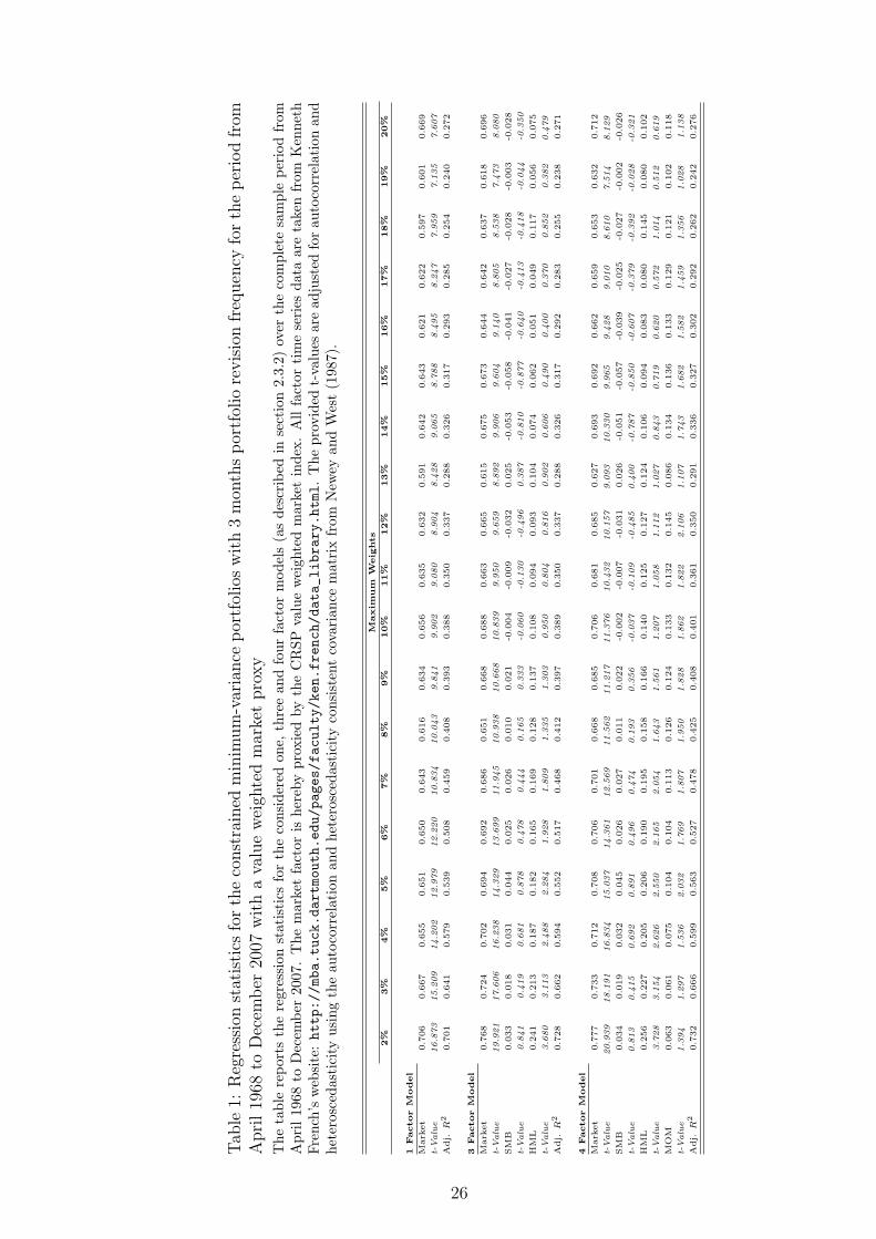
Tab

le1:

Reg

ress

ion

stat

isti

csfo

rth

eco

nst

rain

edm

inim

um

-var

iance

por

tfol

ios

wit

h3

mon

ths

por

tfol

iore

vis

ion

freq

uen

cyfo

rth

ep

erio

dfr

omA

pri

l19

68to

Dec

emb

er20

07w

ith

ava

lue

wei

ghte

dm

arke

tpro

xy

The

tabl

ere

port

sth

ere

gres

sion

stat

isti

csfo

rth

eco

nsid

ered

one,

thre

ean

dfo

urfa

ctor

mod

els

(as

desc

ribe

din

sect

ion

2.3.

2)ov

erth

eco

mpl

ete

sam

ple

peri

odfr

omA

pril

1968

toD

ecem

ber

2007

.T

hem

arke

tfa

ctor

ishe

reby

prox

ied

byth

eC

RSP

valu

ew

eigh

ted

mar

ket

inde

x.A

llfa

ctor

tim

ese

ries

data

are

take

nfr

omK

enne

thFr

ench

’sw

ebsi

te:http://mba.tuck.dartmouth.edu/pages/faculty/ken.french/data_library.html.

The

prov

ided

t-va

lues

are

adju

sted

for

auto

corr

elat

ion

and

hete

rosc

edas

tici

tyus

ing

the

auto

corr

elat

ion

and

hete

rosc

edas

tici

tyco

nsis

tent

cova

rian

cem

atri

xfr

omN

ewey

and

Wes

t(1

987)

.

Maxim

um

Weig

hts

2%

3%

4%

5%

6%

7%

8%

9%

10%

11%

12%

13%

14%

15%

16%

17%

18%

19%

20%

1Factor

Model

Mark

et

0.7

06

0.6

67

0.6

55

0.6

51

0.6

50

0.6

43

0.6

16

0.6

34

0.6

56

0.6

35

0.6

32

0.5

91

0.6

42

0.6

43

0.6

21

0.6

22

0.5

97

0.6

01

0.6

69

t-Valu

e16.8

73

15.2

09

14.2

02

12.9

79

12.2

20

10.8

34

10.0

43

9.8

41

9.9

02

9.0

80

8.9

04

8.4

28

9.0

65

8.7

88

8.4

95

8.2

47

7.9

59

7.1

35

7.6

07

Adj.

R2

0.7

01

0.6

41

0.5

79

0.5

39

0.5

08

0.4

59

0.4

08

0.3

93

0.3

88

0.3

50

0.3

37

0.2

88

0.3

26

0.3

17

0.2

93

0.2

85

0.2

54

0.2

40

0.2

72

3Factor

Model

Mark

et

0.7

68

0.7

24

0.7

02

0.6

94

0.6

92

0.6

86

0.6

51

0.6

68

0.6

88

0.6

63

0.6

65

0.6

15

0.6

75

0.6

73

0.6

44

0.6

42

0.6

37

0.6

18

0.6

96

t-Valu

e19.9

21

17.6

06

16.2

38

14.3

29

13.6

99

11.9

45

10.9

38

10.6

68

10.8

39

9.9

50

9.6

59

8.8

92

9.9

06

9.6

04

9.1

40

8.8

05

8.5

38

7.4

73

8.0

80

SM

B0.0

33

0.0

18

0.0

31

0.0

44

0.0

25

0.0

26

0.0

10

0.0

21

-0.0

04

-0.0

09

-0.0

32

0.0

25

-0.0

53

-0.0

58

-0.0

41

-0.0

27

-0.0

28

-0.0

03

-0.0

28

t-Valu

e0.8

41

0.4

19

0.6

81

0.8

78

0.4

78

0.4

44

0.1

65

0.3

33

-0.0

60

-0.1

30

-0.4

96

0.3

87

-0.8

10

-0.8

77

-0.6

40

-0.4

13

-0.4

18

-0.0

44

-0.3

50

HM

L0.2

41

0.2

13

0.1

87

0.1

82

0.1

65

0.1

69

0.1

28

0.1

37

0.1

08

0.0

94

0.0

93

0.1

04

0.0

74

0.0

62

0.0

51

0.0

49

0.1

17

0.0

56

0.0

75

t-Valu

e3.6

80

3.1

13

2.4

88

2.2

84

1.9

28

1.8

09

1.3

35

1.3

03

0.9

50

0.8

04

0.8

16

0.9

02

0.6

06

0.4

90

0.4

00

0.3

70

0.8

52

0.3

82

0.4

79

Adj.

R2

0.7

28

0.6

62

0.5

94

0.5

52

0.5

17

0.4

68

0.4

12

0.3

97

0.3

89

0.3

50

0.3

37

0.2

88

0.3

26

0.3

17

0.2

92

0.2

83

0.2

55

0.2

38

0.2

71

4Factor

Model

Mark

et

0.7

77

0.7

33

0.7

12

0.7

08

0.7

06

0.7

01

0.6

68

0.6

85

0.7

06

0.6

81

0.6

85

0.6

27

0.6

93

0.6

92

0.6

62

0.6

59

0.6

53

0.6

32

0.7

12

t-Valu

e20.9

39

18.1

91

16.8

34

15.0

37

14.3

61

12.5

69

11.5

62

11.2

17

11.3

76

10.4

32

10.1

57

9.0

93

10.3

30

9.9

65

9.4

28

9.0

10

8.6

10

7.5

14

8.1

29

SM

B0.0

34

0.0

19

0.0

32

0.0

45

0.0

26

0.0

27

0.0

11

0.0

22

-0.0

02

-0.0

07

-0.0

31

0.0

26

-0.0

51

-0.0

57

-0.0

39

-0.0

25

-0.0

27

-0.0

02

-0.0

26

t-Valu

e0.8

13

0.4

15

0.6

92

0.8

91

0.4

96

0.4

74

0.1

93

0.3

56

-0.0

37

-0.1

09

-0.4

85

0.4

00

-0.7

87

-0.8

50

-0.6

07

-0.3

79

-0.3

92

-0.0

28

-0.3

21

HM

L0.2

56

0.2

27

0.2

05

0.2

06

0.1

90

0.1

95

0.1

58

0.1

66

0.1

40

0.1

25

0.1

27

0.1

24

0.1

06

0.0

94

0.0

83

0.0

80

0.1

45

0.0

80

0.1

02

t-Valu

e3.7

28

3.1

54

2.6

26

2.5

50

2.1

65

2.0

54

1.6

43

1.5

61

1.2

07

1.0

58

1.1

12

1.0

27

0.8

43

0.7

19

0.6

20

0.5

72

1.0

14

0.5

12

0.6

19

MO

M0.0

63

0.0

61

0.0

75

0.1

04

0.1

04

0.1

13

0.1

26

0.1

24

0.1

33

0.1

32

0.1

45

0.0

86

0.1

34

0.1

36

0.1

33

0.1

29

0.1

21

0.1

02

0.1

18

t-Valu

e1.3

94

1.2

97

1.5

36

2.0

32

1.7

69

1.8

07

1.9

50

1.8

28

1.8

62

1.8

22

2.1

06

1.1

07

1.7

43

1.6

82

1.5

82

1.4

59

1.3

56

1.0

28

1.1

38

Adj.

R2

0.7

32

0.6

66

0.5

99

0.5

63

0.5

27

0.4

78

0.4

25

0.4

08

0.4

01

0.3

61

0.3

50

0.2

91

0.3

36

0.3

27

0.3

02

0.2

92

0.2

62

0.2

42

0.2

76

26

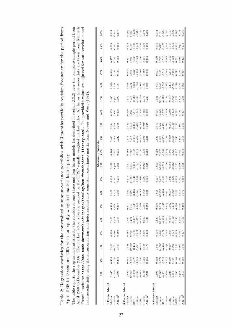
Tab

le2:

Reg

ress

ion

stat

isti

csfo

rth

eco

nst

rain

edm

inim

um

-var

iance

por

tfol

ios

wit

h3

mon

ths

por

tfol

iore

vis

ion

freq

uen

cyfo

rth

ep

erio

dfr

omA

pri

l19

68to

Dec

emb

er20

07w

ith

aneq

ual

lyw

eigh

ted

mar

ket

fact

orpro

xy

The

tabl

ere

port

sth

ere

gres

sion

stat

isti

csfo

rth

eco

nsid

ered

one,

thre

ean

dfo

urfa

ctor

mod

els

(as

desc

ribe

din

sect

ion

2.3.

2)ov

erth

eco

mpl

ete

sam

ple

peri

odfr

omA

pril

1968

toD

ecem

ber

2007

.T

hem

arke

tfa

ctor

ishe

reby

prox

ied

byth

eC

RSP

equa

llyw

eigh

ted

mar

ket

inde

x.A

llfa

ctor

tim

ese

ries

data

are

take

nfr

omK

enne

thFr

ench

’sw

ebsi

te:http://mba.tuck.dartmouth.edu/pages/faculty/ken.french/data_library.html.

The

prov

ided

t-va

lues

are

adju

sted

for

auto

corr

elat

ion

and

hete

rosc

edas

tici

tyus

ing

the

auto

corr

elat

ion

and

hete

rosc

edas

tici

tyco

nsis

tent

cova

rian

cem

atri

xfr

omN

ewey

and

Wes

t(1

987)

.

Maxim

um

Weig

hts

2%

3%

4%

5%

6%

7%

8%

9%

10%

11%

12%

13%

14%

15%

16%

17%

18%

19%

20%

1Factor

Model

Mark

et

0.4

65

0.4

35

0.4

29

0.4

28

0.4

26

0.4

19

0.4

01

0.4

16

0.4

26

0.4

08

0.4

03

0.3

94

0.4

03

0.4

00

0.3

90

0.3

94

0.3

77

0.3

89

0.4

24

t-Valu

e11.2

69

10.7

56

10.4

74

9.8

80

9.3

58

8.6

56

8.1

19

8.3

21

8.4

08

7.8

75

7.6

69

7.5

88

7.6

75

7.4

81

7.2

21

7.1

72

6.7

90

6.5

31

6.5

63

Adj.

R2

0.4

95

0.4

44

0.4

04

0.3

80

0.3

54

0.3

17

0.2

80

0.2

76

0.2

66

0.2

35

0.2

22

0.2

08

0.2

08

0.1

99

0.1

87

0.1

85

0.1

63

0.1

63

0.1

77

3Factor

Model

Mark

et

0.6

52

0.6

13

0.5

91

0.5

83

0.5

87

0.5

77

0.5

53

0.5

71

0.5

91

0.5

65

0.5

71

0.5

35

0.5

76

0.5

72

0.5

46

0.5

45

0.5

37

0.5

28

0.5

90

t-Valu

e12.3

63

11.5

68

10.6

92

9.7

38

9.4

74

8.5

01

8.1

09

8.1

86

8.3

59

7.8

12

7.7

51

7.5

46

7.9

24

7.7

49

7.4

34

7.2

55

7.0

82

6.4

37

6.6

55

SM

B-0

.492

-0.4

76

-0.4

44

-0.4

24

-0.4

47

-0.4

38

-0.4

36

-0.4

40

-0.4

82

-0.4

65

-0.4

94

-0.4

10

-0.5

18

-0.5

19

-0.4

81

-0.4

66

-0.4

60

-0.4

30

-0.5

03

t-Valu

e-6

.288

-5.9

98

-5.0

13

-4.4

35

-4.5

53

-3.9

82

-3.9

12

-3.8

98

-4.1

43

-3.8

14

-4.0

66

-3.6

39

-4.2

87

-4.2

60

-4.1

28

-3.9

96

-4.0

05

-3.4

27

-3.8

72

HM

L-0

.012

-0.0

26

-0.0

45

-0.0

48

-0.0

63

-0.0

58

-0.0

85

-0.0

81

-0.1

16

-0.1

24

-0.1

23

-0.0

94

-0.1

47

-0.1

59

-0.1

60

-0.1

62

-0.0

94

-0.1

46

-0.1

54

t-Valu

e-0

.152

-0.3

22

-0.5

15

-0.5

30

-0.6

61

-0.5

69

-0.8

09

-0.7

20

-0.9

48

-0.9

85

-1.0

12

-0.7

89

-1.1

24

-1.1

71

-1.1

95

-1.1

80

-0.6

80

-0.9

81

-0.9

71

Adj.

R2

0.5

91

0.5

35

0.4

79

0.4

43

0.4

21

0.3

76

0.3

37

0.3

28

0.3

25

0.2

89

0.2

81

0.2

45

0.2

69

0.2

60

0.2

39

0.2

33

0.2

04

0.1

98

0.2

21

4Factor

Model

Mark

et

0.6

94

0.6

52

0.6

34

0.6

33

0.6

37

0.6

30

0.6

08

0.6

27

0.6

50

0.6

23

0.6

33

0.5

79

0.6

35

0.6

31

0.6

04

0.6

01

0.5

90

0.5

76

0.6

44

t-Valu

e17.3

79

15.6

77

14.4

70

13.2

50

12.9

07

11.3

11

10.9

03

10.6

78

10.9

99

10.0

15

9.9

68

9.3

63

10.4

08

10.1

04

9.5

62

9.1

90

8.7

67

7.8

47

8.1

21

SM

B-0

.531

-0.5

12

-0.4

84

-0.4

71

-0.4

95

-0.4

87

-0.4

88

-0.4

93

-0.5

38

-0.5

19

-0.5

52

-0.4

51

-0.5

73

-0.5

75

-0.5

35

-0.5

18

-0.5

10

-0.4

75

-0.5

54

t-Valu

e-7

.690

-7.2

15

-6.2

49

-5.6

82

-5.8

61

-5.1

34

-5.0

71

-5.0

87

-5.4

56

-4.9

34

-5.4

19

-4.5

85

-5.5

59

-5.4

72

-5.2

97

-5.0

88

-5.2

03

-4.1

83

-4.7

66

HM

L0.0

25

0.0

09

-0.0

07

-0.0

04

-0.0

18

-0.0

12

-0.0

37

-0.0

33

-0.0

64

-0.0

73

-0.0

69

-0.0

56

-0.0

95

-0.1

07

-0.1

10

-0.1

13

-0.0

47

-0.1

04

-0.1

07

t-Valu

e0.2

99

0.1

03

-0.0

82

-0.0

41

-0.1

90

-0.1

17

-0.3

48

-0.2

86

-0.5

18

-0.5

80

-0.5

69

-0.4

48

-0.7

13

-0.7

69

-0.7

94

-0.7

86

-0.3

25

-0.6

56

-0.6

34

MO

M0.1

56

0.1

48

0.1

60

0.1

89

0.1

90

0.1

98

0.2

09

0.2

10

0.2

23

0.2

17

0.2

33

0.1

66

0.2

22

0.2

22

0.2

16

0.2

12

0.2

01

0.1

81

0.2

05

t-Valu

e2.4

88

2.3

58

2.5

01

2.8

78

2.6

26

2.5

90

2.6

89

2.5

94

2.6

08

2.5

35

2.8

56

1.8

60

2.4

61

2.3

72

2.2

33

2.1

02

1.9

88

1.6

44

1.7

71

Adj.

R2

0.6

17

0.5

58

0.5

04

0.4

77

0.4

53

0.4

08

0.3

72

0.3

60

0.3

58

0.3

19

0.3

14

0.2

61

0.2

97

0.2

88

0.2

65

0.2

57

0.2

25

0.2

13

0.2

39

27

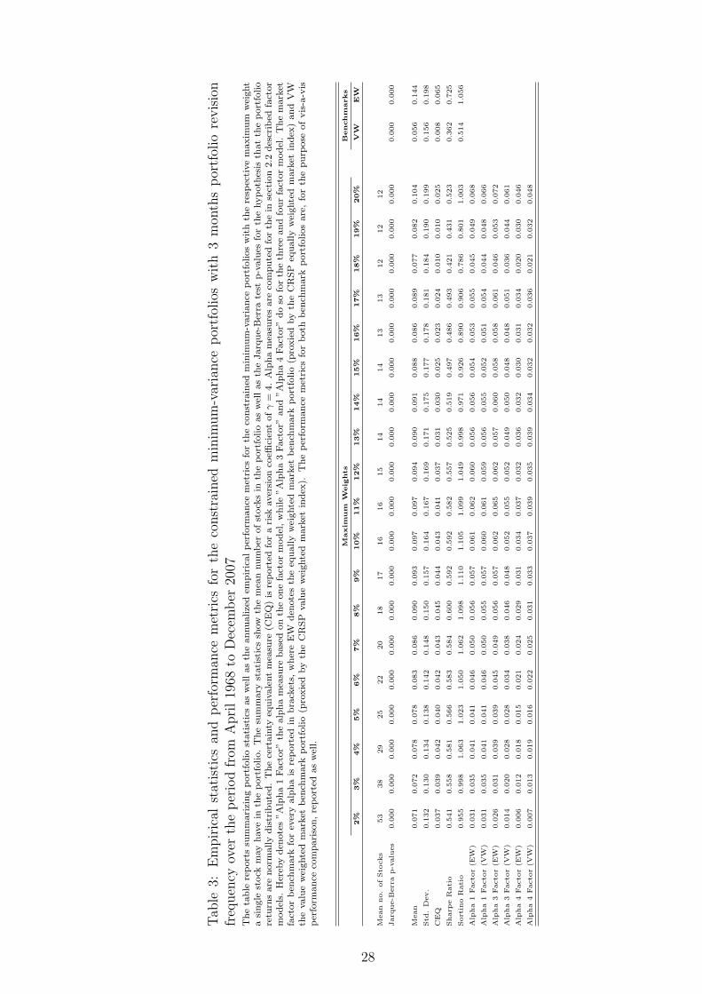
Tab

le3:

Em

pir

ical

stat

isti

csan

dp

erfo

rman

cem

etri

csfo

rth

eco

nst

rain

edm

inim

um

-var

iance

por

tfol

ios

wit

h3

mon

ths

por

tfol

iore

vis

ion

freq

uen

cyov

erth

ep

erio

dfr

omA

pri

l19

68to

Dec

emb

er20

07T

he

tab

lere

port

ssu

mm

ari

zin

gp

ort

folio

stati

stic

sas

wel

las

the

an

nu

alize

dem

pir

ical

per

form

an

cem

etri

csfo

rth

eco

nst

rain

edm

inim

um

-vari

an

cep

ort

folios

wit

hth

ere

spec

tive

maxim

um

wei

ght

asi

ngle

stock

may

have

inth

ep

ort

folio.

Th

esu

mm

ary

stati

stic

ssh

ow

the

mea

nnum

ber

of

stock

sin

the

port

foli

oas

wel

las

the

Jarq

ue-

Ber

rate

stp

-valu

esfo

rth

ehyp

oth

esis

that

the

port

folio

retu

rns

are

norm

ally

dis

trib

ute

d.

Th

ece

rtain

tyeq

uiv

ale

nt

mea

sure

(CE

Q)

isre

port

edfo

ra

risk

aver

sion

coeffi

cien

tofγ

=4.

Alp

ha

mea

sure

sare

com

pu

ted

for

the

inse

ctio

n2.2

des

crib

edfa

ctor

mod

els.

Her

eby

den

ote

s”A

lph

a1

Fact

or”

the

alp

ha

mea

sure

base

don

the

on

efa

ctor

mod

el,

wh

ile

”A

lph

a3

Fact

or”

an

d”A

lph

a4

Fact

or”

do

sofo

rth

eth

ree

an

dfo

ur

fact

or

mod

el.

Th

em

ark

etfa

ctor

ben

chm

ark

for

ever

yalp

ha

isre

port

edin

bra

cket

s,w

her

eE

Wd

enote

sth

eeq

ually

wei

ghte

dm

ark

etb

ench

mark

port

folio

(pro

xie

dby

the

CR

SP

equ

ally

wei

ghte

dm

ark

etin

dex

)an

dV

Wth

evalu

ew

eighte

dm

ark

etb

ench

mark

port

folio

(pro

xie

dby

the

CR

SP

valu

ew

eighte

dm

ark

etin

dex

).T

he

per

form

an

cem

etri

csfo

rb

oth

ben

chm

ark

port

foli

os

are

,fo

rth

ep

urp

ose

of

vis

-a-v

isp

erfo

rman

ceco

mp

ari

son

,re

port

edas

wel

l.

Maxim

um

Weig

hts

Benchm

arks

2%

3%

4%

5%

6%

7%

8%

9%

10%

11%

12%

13%

14%

15%

16%

17%

18%

19%

20%

VW

EW

Mean

no.

of

Sto

cks

53

38

29

25

22

20

18

17

16

16

15

14

14

14

13

13

12

12

12

Jarq

ue-B

err

ap-v

alu

es

0.0

00

0.0

00

0.0

00

0.0

00

0.0

00

0.0

00

0.0

00

0.0

00

0.0

00

0.0

00

0.0

00

0.0

00

0.0

00

0.0

00

0.0

00

0.0

00

0.0

00

0.0

00

0.0

00

0.0

00

0.0

00

Mean

0.0

71

0.0

72

0.0

78

0.0

78

0.0

83

0.0

86

0.0

90

0.0

93

0.0

97

0.0

97

0.0

94

0.0

90

0.0

91

0.0

88

0.0

86

0.0

89

0.0

77

0.0

82

0.1

04

0.0

56

0.1

44

Std

.D

ev.

0.1

32

0.1

30

0.1

34

0.1

38

0.1

42

0.1

48

0.1

50

0.1

57

0.1

64

0.1

67

0.1

69

0.1

71

0.1

75

0.1

77

0.1

78

0.1

81

0.1

84

0.1

90

0.1

99

0.1

56

0.1

98

CE

Q0.0

37

0.0

39

0.0

42

0.0

40

0.0

42

0.0

43

0.0

45

0.0

44

0.0

43

0.0

41

0.0

37

0.0

31

0.0

30

0.0

25

0.0

23

0.0

24

0.0

10

0.0

10

0.0

25

0.0

08

0.0

65

Sharp

eR

ati

o0.5

41

0.5

58

0.5

81

0.5

66

0.5

83

0.5

84

0.6

00

0.5

92

0.5

92

0.5

82

0.5

57

0.5

25

0.5

19

0.4

97

0.4

86

0.4

93

0.4

21

0.4

31

0.5

23

0.3

62

0.7

25

Sort

ino

Rati

o0.9

55

0.9

98

1.0

63

1.0

23

1.0

50

1.0

62

1.0

98

1.1

10

1.1

05

1.0

99

1.0

49

0.9

98

0.9

71

0.9

26

0.8

90

0.9

06

0.7

86

0.8

01

1.0

03

0.5

14

1.0

56

Alp

ha

1Facto

r(E

W)

0.0

31

0.0

35

0.0

41

0.0

41

0.0

46

0.0

50

0.0

56

0.0

57

0.0

61

0.0

62

0.0

60

0.0

56

0.0

56

0.0

54

0.0

53

0.0

55

0.0

45

0.0

49

0.0

68

Alp

ha

1Facto

r(V

W)

0.0

31

0.0

35

0.0

41

0.0

41

0.0

46

0.0

50

0.0

55

0.0

57

0.0

60

0.0

61

0.0

59

0.0

56

0.0

55

0.0

52

0.0

51

0.0

54

0.0

44

0.0

48

0.0

66

Alp

ha

3Facto

r(E

W)

0.0

26

0.0

31

0.0

39

0.0

39

0.0

45

0.0

49

0.0

56

0.0

57

0.0

62

0.0

65

0.0

62

0.0

57

0.0

60

0.0

58

0.0

58

0.0

61

0.0

46

0.0

53

0.0

72

Alp

ha

3Facto

r(V

W)

0.0

14

0.0

20

0.0

28

0.0

28

0.0

34

0.0

38

0.0

46

0.0

48

0.0

52

0.0

55

0.0

52

0.0

49

0.0

50

0.0

48

0.0

48

0.0

51

0.0

36

0.0

44

0.0

61

Alp

ha

4Facto

r(E

W)

0.0

06

0.0

12

0.0

18

0.0

15

0.0

21

0.0

24

0.0

29

0.0

31

0.0

34

0.0

37

0.0

32

0.0

36

0.0

32

0.0

30

0.0

31

0.0

34

0.0

20

0.0

30

0.0

46

Alp

ha

4Facto

r(V

W)

0.0

07

0.0

13

0.0

19

0.0

16

0.0

22

0.0

25

0.0

31

0.0

33

0.0

37

0.0

39

0.0

35

0.0

39

0.0

34

0.0

32

0.0

32

0.0

36

0.0

21

0.0

32

0.0

48

28

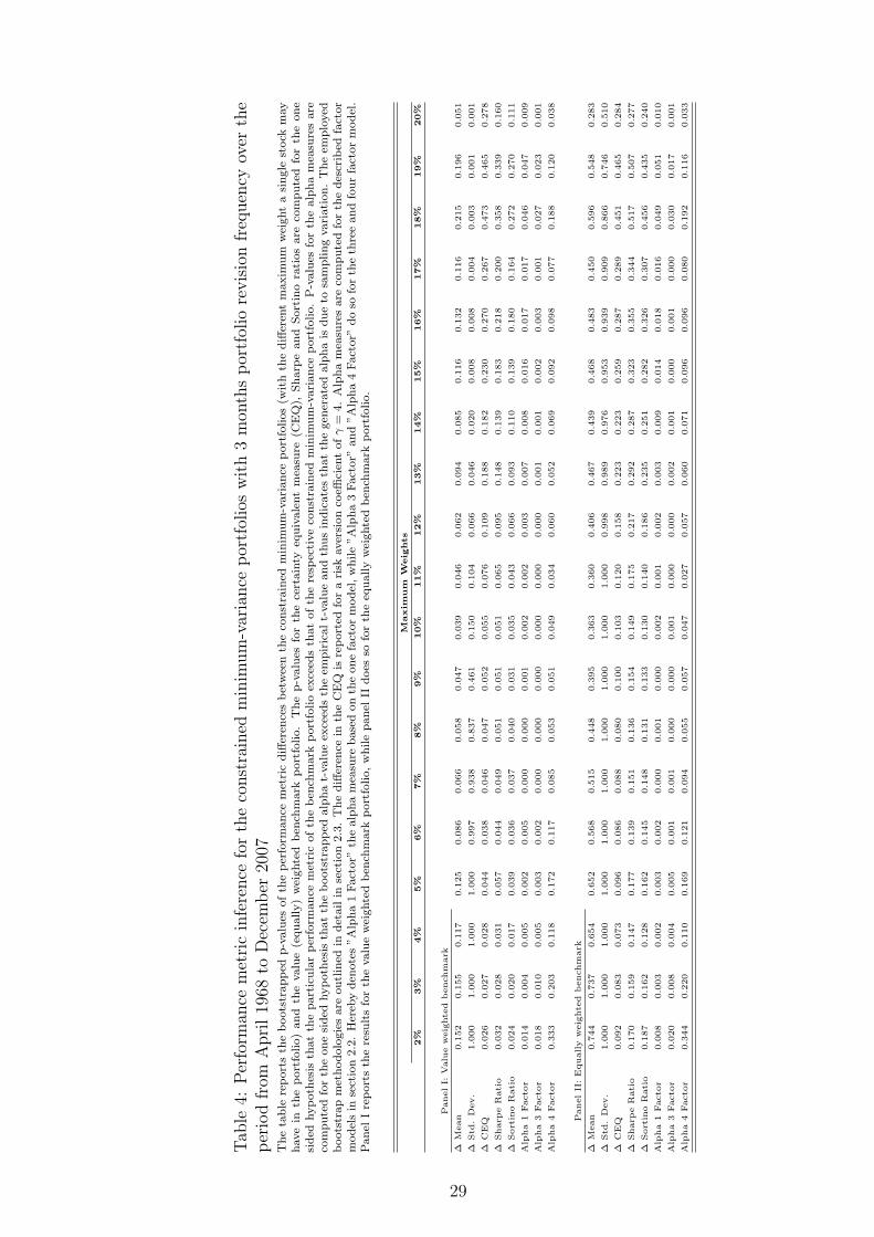
Tab

le4:

Per

form

ance

met

ric

infe

rence

for

the

const

rain

edm

inim

um

-var

iance

por

tfol

ios

wit

h3

mon

ths

por

tfol

iore

vis

ion

freq

uen

cyov

erth

ep

erio

dfr

omA

pri

l19

68to

Dec

emb

er20

07T

he

tab

lere

port

sth

eb

oots

trap

ped

p-v

alu

esof

the

per

form

an

cem

etri

cd

iffer

ence

sb

etw

een

the

con

stra

ined

min

imu

m-v

ari

an

cep

ort

folios

(wit

hth

ed

iffer

ent

maxim

um

wei

ght

asi

ngle

stock

may

have

inth

ep

ort

folio)

an

dth

evalu

e(e

qu

ally)

wei

ghte

db

ench

mark

port

folio.

Th

ep

-valu

esfo

rth

ece

rtain

tyeq

uiv

ale

nt

mea

sure

(CE

Q),

Sh

arp

ean

dS

ort

ino

rati

os

are

com

pu

ted

for

the

on

esi

ded

hyp

oth

esis

that

the

part

icu

lar

per

form

an

cem

etri

cof

the

ben

chm

ark

port

folio

exce

eds

that

of

the

resp

ecti

ve

con

stra

ined

min

imu

m-v

ari

an

cep

ort

folio.

P-v

alu

esfo

rth

ealp

ha

mea

sure

sare

com

pu

ted

for

the

on

esi

ded

hyp

oth

esis

that

the

boots

trap

ped

alp

ha

t-valu

eex

ceed

sth

eem

pir

ical

t-valu

ean

dth

us

ind

icate

sth

at

the

gen

erate

dalp

ha

isd

ue

tosa

mp

lin

gvari

ati

on

.T

he

emp

loyed

boots

trap

met

hod

olo

gie

sare

ou

tlin

edin

det

ail

inse

ctio

n2.3

.T

he

diff

eren

cein

the

CE

Qis

rep

ort

edfo

ra

risk

aver

sion

coeffi

cien

tofγ

=4.

Alp

ha

mea

sure

sare

com

pu

ted

for

the

des

crib

edfa

ctor

mod

els

inse

ctio

n2.2

.H

ereb

yd

enote

s”A

lph

a1

Fact

or”

the

alp

ha

mea

sure

base

don

the

on

efa

ctor

mod

el,

wh

ile

”A

lph

a3

Fact

or”

an

d”A

lph

a4

Fact

or”

do

sofo

rth

eth

ree

an

dfo

ur

fact

or

mod

el.

Pan

elI

rep

ort

sth

ere

sult

sfo

rth

evalu

ew

eighte

db

ench

mark

port

folio,

wh

ile

pan

elII

does

sofo

rth

eeq

ually

wei

ghte

db

ench

mark

port

folio.

Maxim

um

Weig

hts

2%

3%

4%

5%

6%

7%

8%

9%

10%

11%

12%

13%

14%

15%

16%

17%

18%

19%

20%

Panel

I:V

alu

ew

eig

hte

db

enchm

ark

∆M

ean

0.1

52

0.1

55

0.1

17

0.1

25

0.0

86

0.0

66

0.0

58

0.0

47

0.0

39

0.0

46

0.0

62

0.0

94

0.0

85

0.1

16

0.1

32

0.1

16

0.2

15

0.1

96

0.0

51

∆Std

.D

ev.

1.0

00

1.0

00

1.0

00

1.0

00

0.9

97

0.9

38

0.8

37

0.4

61

0.1

50

0.1

04

0.0

66

0.0

46

0.0

20

0.0

08

0.0

08

0.0

04

0.0

03

0.0

01

0.0

01

∆C

EQ

0.0

26

0.0

27

0.0

28

0.0

44

0.0

38

0.0

46

0.0

47

0.0

52

0.0

55

0.0

76

0.1

09

0.1

88

0.1

82

0.2

30

0.2

70

0.2

67

0.4

73

0.4

65

0.2

78

∆Sharp

eR

ati

o0.0

32

0.0

28

0.0

31

0.0

57

0.0

44

0.0

49

0.0

51

0.0

51

0.0

51

0.0

65

0.0

95

0.1

48

0.1

39

0.1

83

0.2

18

0.2

00

0.3

58

0.3

39

0.1

60

∆Sort

ino

Rati

o0.0

24

0.0

20

0.0

17

0.0

39

0.0

36

0.0

37

0.0

40

0.0

31

0.0

35

0.0

43

0.0

66

0.0

93

0.1

10

0.1

39

0.1

80

0.1

64

0.2

72

0.2

70

0.1

11

Alp

ha

1Facto

r0.0

14

0.0

04

0.0

05

0.0

02

0.0

05

0.0

00

0.0

00

0.0

01

0.0

02

0.0

02

0.0

03

0.0

07

0.0

08

0.0

16

0.0

17

0.0

17

0.0

46

0.0

47

0.0

09

Alp

ha

3Facto

r0.0

18

0.0

10

0.0

05

0.0

03

0.0

02

0.0

00

0.0

00

0.0

00

0.0

00

0.0

00

0.0

00

0.0

01

0.0

01

0.0

02

0.0

03

0.0

01

0.0

27

0.0

23

0.0

01

Alp

ha

4Facto

r0.3

33

0.2

03

0.1

18

0.1

72

0.1

17

0.0

85

0.0

53

0.0

51

0.0

49

0.0

34

0.0

60

0.0

52

0.0

69

0.0

92

0.0

98

0.0

77

0.1

88

0.1

20

0.0

38

Panel

II:

Equall

yw

eig

hte

db

enchm

ark

∆M

ean

0.7

44

0.7

37

0.6

54

0.6

52

0.5

68

0.5

15

0.4

48

0.3

95

0.3

63

0.3

60

0.4

06

0.4

67

0.4

39

0.4

68

0.4

83

0.4

50

0.5

96

0.5

48

0.2

83

∆Std

.D

ev.

1.0

00

1.0

00

1.0

00

1.0

00

1.0

00

1.0

00

1.0

00

1.0

00

1.0

00

1.0

00

0.9

98

0.9

89

0.9

76

0.9

53

0.9

39

0.9

09

0.8

66

0.7

46

0.5

10

∆C

EQ

0.0

92

0.0

83

0.0

73

0.0

96

0.0

86

0.0

88

0.0

80

0.1

00

0.1

03

0.1

20

0.1

58

0.2

23

0.2

23

0.2

59

0.2

87

0.2

89

0.4

51

0.4

65

0.2

84

∆Sharp

eR

ati

o0.1

70

0.1

59

0.1

47

0.1

77

0.1

39

0.1

51

0.1

36

0.1

54

0.1

49

0.1

75

0.2

17

0.2

92

0.2

87

0.3

23

0.3

55

0.3

44

0.5

17

0.5

07

0.2

77

∆Sort

ino

Rati

o0.1

87

0.1

62

0.1

28

0.1

62

0.1

45

0.1

48

0.1

31

0.1

33

0.1

30

0.1

40

0.1

86

0.2

35

0.2

51

0.2

82

0.3

26

0.3

07

0.4

56

0.4

35

0.2

40

Alp

ha

1Facto

r0.0

08

0.0

03

0.0

02

0.0

03

0.0

02

0.0

00

0.0

01

0.0

00

0.0

02

0.0

01

0.0

02

0.0

03

0.0

09

0.0

14

0.0

18

0.0

16

0.0

49

0.0

51

0.0

10

Alp

ha

3Facto

r0.0

20

0.0

08

0.0

04

0.0

05

0.0

01

0.0

01

0.0

00

0.0

00

0.0

01

0.0

00

0.0

00

0.0

02

0.0

01

0.0

00

0.0

01

0.0

00

0.0

30

0.0

17

0.0

01

Alp

ha

4Facto

r0.3

44

0.2

20

0.1

10

0.1

69

0.1

21

0.0

94

0.0

55

0.0

57

0.0

47

0.0

27

0.0

57

0.0

60

0.0

71

0.0

96

0.0

96

0.0

80

0.1

92

0.1

16

0.0

33

29

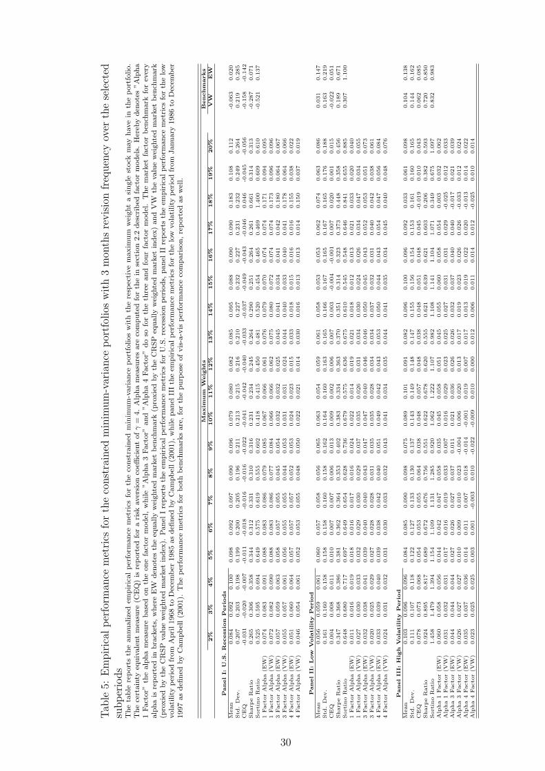
Tab

le5:

Em

pir

ical

per

form

ance

met

rics

for

the

const

rain

edm

inim

um

-var

iance

por

tfol

ios

wit

h3

mon

ths

revis

ion

freq

uen

cyov

erth

ese

lect

edsu

bp

erio

ds

Th

eta

ble

rep

ort

sth

ean

nu

alize

dem

pir

ical

per

form

an

cem

etri

csfo

rth

eco

nst

rain

edm

inim

um

-vari

an

cep

ort

foli

os

wit

hth

ere

spec

tive

maxim

um

wei

ght

asi

ngle

stock

may

have

inth

ep

ort

folio.

Th

ece

rtain

tyeq

uiv

ale

nt

mea

sure

(CE

Q)

isre

port

edfo

ra

risk

aver

sion

coeffi

cien

tofγ

=4.

Alp

ha

mea

sure

sare

com

pu

ted

for

the

inse

ctio

n2.2

des

crib

edfa

ctor

mod

els.

Her

eby

den

ote

s”A

lph

a1

Fact

or”

the

alp

ha

mea

sure

base

don

the

on

efa

ctor

mod

el,

wh

ile

”A

lph

a3

Fact

or”

an

d”A

lph

a4

Fact

or”

do

sofo

rth

eth

ree

an

dfo

ur

fact

or

mod

el.

Th

em

ark

etfa

ctor

ben

chm

ark

for

ever

yalp

ha

isre

port

edin

bra

cket

s,w

her

eE

Wd

enote

sth

eeq

ually

wei

ghte

dm

ark

etb

ench

mark

(pro

xie

dby

the

CR

SP

equ

ally

wei

ghte

dm

ark

etin

dex

)an

dV

Wth

evalu

ew

eighte

dm

ark

etb

ench

mark

(pro

xie

dby

the

CR

SP

valu

ew

eighte

dm

ark

etin

dex

).P

an

elI

rep

ort

sth

eem

pir

ical

per

form

an

cem

etri

csfo

rU

.S.

rece

ssio

np

erio

ds,

pan

elII

rep

ort

sth

eem

pir

ical

per

form

an

cem

etri

csfo

rth

elo

wvola

tili

typ

erio

dfr

om

Ap

ril

1968

toD

ecem

ber

1985

as

defi

ned

by

Cam

pb

ell

(2001),

wh

ile

pan

elII

Ith

eem

pir

ical

per

form

an

cem

etri

csfo

rth

elo

wvola

tility

per

iod

from

Janu

ary

1986

toD

ecem

ber

1997

as

defi

ned

by

Cam

pb

ell

(2001).

Th

ep

erfo

rman

cem

etri

csfo

rb

oth

ben

chm

ark

sare

,fo

rth

ep

urp

ose

of

vis

-a-v

isp

erfo

rman

ceco

mp

ari

son

,re

port

edas

wel

l.

Maxim

um

Weig

hts

Benchm

arks

2%

3%

4%

5%

6%

7%

8%

9%

10%

11%

12%

13%

14%

15%

16%

17%

18%

19%

20%

VW

EW

PanelI:U

.S.R

ecessio

nPerio

ds

Mean

0.0

84

0.0

92

0.1

00

0.0

98

0.0

92

0.0

97

0.0

90

0.0

96

0.0

79

0.0

80

0.0

82

0.0

85

0.0

95

0.0

88

0.0

90

0.0

90

0.1

83

0.1

08

0.1

12

-0.0

63

0.0

20

Std

.D

ev.

0.2

07

0.2

03

0.1

98

0.1

99

0.2

00

0.2

05

0.1

96

0.2

11

0.2

13

0.2

15

0.2

16

0.2

10

0.2

27

0.2

32

0.2

27

0.2

31

0.2

32

0.2

49

0.2

64

0.2

19

0.2

85

CE

Q-0

.031

-0.0

20

-0.0

07

-0.0

11

-0.0

18

-0.0

16

-0.0

16

-0.0

22

-0.0

41

-0.0

42

-0.0

40

-0.0

33

-0.0

37

-0.0

49

-0.0

43

-0.0

46

0.0

46

-0.0

45

-0.0

56

-0.1

58

-0.1

42

Sharp

eR

ati

o0.2

65

0.3

06

0.3

58

0.3

44

0.3

12

0.3

31

0.3

10

0.3

16

0.2

31

0.2

34

0.2

45

0.2

64

0.2

90

0.2

51

0.2

64

0.2

61

0.6

61

0.3

14

0.3

13

-0.2

87

0.0

71

Sort

ino

Rati

o0.5

25

0.5

95

0.6

94

0.6

49

0.5

75

0.6

19

0.5

55

0.6

02

0.4

18

0.4

15

0.4

50

0.4

81

0.5

20

0.4

54

0.4

65

0.4

69

1.4

00

0.6

09

0.6

10

-0.5

21

0.1

37

1Facto

rA

lpha

(EW

)0.0

74

0.0

83

0.0

91

0.0

88

0.0

83

0.0

86

0.0

79

0.0

85

0.0

67

0.0

66

0.0

61

0.0

76

0.0

79

0.0

70

0.0

74

0.0

74

0.1

71

0.0

94

0.0

95

1Facto

rA

lpha

(VW

)0.0

72

0.0

82

0.0

90

0.0

88

0.0

83

0.0

86

0.0

77

0.0

84

0.0

66

0.0

66

0.0

62

0.0

75

0.0

80

0.0

72

0.0

74

0.0

74

0.1

73

0.0

96

0.0

96

3Facto

rA

lpha

(EW

)0.0

57

0.0

59

0.0

63

0.0

58

0.0

57

0.0

55

0.0

45

0.0

54

0.0

32

0.0

32

0.0

25

0.0

45

0.0

41

0.0

34

0.0

41

0.0

42

0.1

80

0.0

64

0.0

67

3Facto

rA

lpha

(VW

)0.0

55

0.0

57

0.0

61

0.0

56

0.0

55

0.0

55

0.0

44

0.0

53

0.0

31

0.0

31

0.0

24

0.0

44

0.0

40

0.0

33

0.0

40

0.0

41

0.1

78

0.0

64

0.0

66

4Facto

rA

lpha

(EW

)0.0

51

0.0

60

0.0

64

0.0

57

0.0

57

0.0

57

0.0

52

0.0

53

0.0

24

0.0

23

0.0

15

0.0

33

0.0

18

0.0

15

0.0

16

0.0

16

0.1

55

0.0

38

0.0

22

4Facto

rA

lpha

(VW

)0.0

46

0.0

54

0.0

61

0.0

52

0.0

53

0.0

55

0.0

48

0.0

50

0.0

22

0.0

21

0.0

14

0.0

30

0.0

16

0.0

13

0.0

13

0.0

14

0.1

50

0.0

37

0.0

19

PanelII:Low

Vola

tility

Perio

dM

ean

0.0

56

0.0

59

0.0

61

0.0

60

0.0

57

0.0

58

0.0

56

0.0

65

0.0

63

0.0

54

0.0

59

0.0

61

0.0

58

0.0

53

0.0

53

0.0

62

0.0

74

0.0

63

0.0

86

0.0

31

0.1

47

Std

.D

ev.

0.1

61

0.1

60

0.1

58

0.1

58

0.1

58

0.1

60

0.1

58

0.1

62

0.1

64

0.1

60

0.1

63

0.1

65

0.1

66

0.1

67

0.1

65

0.1

67

0.1

65

0.1

76

0.1

88

0.1

63

0.2

19

CE

Q0.0

04

0.0

08

0.0

11

0.0

10

0.0

07

0.0

07

0.0

06

0.0

13

0.0

09

0.0

02

0.0

06

0.0

07

0.0

03

-0.0

04

-0.0

01

0.0

07

0.0

20

0.0

01

0.0

15

-0.0

22

0.0

51

Sharp

eR

ati

o0.3

47

0.3

68

0.3

86

0.3

81

0.3

62

0.3

64

0.3

53

0.4

02

0.3

83

0.3

34

0.3

63

0.3

70

0.3

51

0.3

14

0.3

23

0.3

73

0.4

48

0.3

58

0.4

56

0.1

89

0.6

71

Sort

ino

Rati

o0.6

48

0.6

80

0.7

17

0.6

97

0.6

49

0.6

54

0.6

28

0.7

36

0.6

79

0.5

75

0.6

36

0.6

75

0.6

10

0.5

45

0.5

48

0.6

46

0.8

41

0.6

55

0.8

85

0.3

07

1.1

00

1Facto

rA

lpha

(EW

)0.0

11

0.0

16

0.0

19

0.0

18

0.0

16

0.0

17

0.0

16

0.0

24

0.0

22

0.0

14

0.0

19

0.0

21

0.0

18

0.0

12

0.0

13

0.0

21

0.0

33

0.0

20

0.0

40

1Facto

rA

lpha

(VW

)0.0

27

0.0

30

0.0

33

0.0

32

0.0

29

0.0

30

0.0

29

0.0

37

0.0

35

0.0

26

0.0

31

0.0

34

0.0

30

0.0

24

0.0

26

0.0

34

0.0

47

0.0

34

0.0

55

3Facto

rA

lpha

(EW

)0.0

32

0.0

38

0.0

41

0.0

39

0.0

40

0.0

40

0.0

43

0.0

47

0.0

47

0.0

40

0.0

46

0.0

46

0.0

50

0.0

45

0.0

43

0.0

52

0.0

53

0.0

51

0.0

73

3Facto

rA

lpha

(VW

)0.0

20

0.0

25

0.0

29

0.0

27

0.0

28

0.0

28

0.0

31

0.0

35

0.0

35

0.0

28

0.0

34

0.0

34

0.0

37

0.0

32

0.0

31

0.0

40

0.0

42

0.0

38

0.0

61

4Facto

rA

lpha

(EW

)0.0

33

0.0

39

0.0

40

0.0

39

0.0

38

0.0

42

0.0

40

0.0

51

0.0

49

0.0

42

0.0

43

0.0

53

0.0

50

0.0

44

0.0

43

0.0

54

0.0

47

0.0

56

0.0

84

4Facto

rA

lpha

(VW

)0.0

24

0.0

31

0.0

32

0.0

31

0.0

30

0.0

33

0.0

32

0.0

43

0.0

41

0.0

34

0.0

35

0.0

44

0.0

41

0.0

35

0.0

34

0.0

45

0.0

40

0.0

48

0.0

76

PanelIII:H

igh

Vola

tility

Perio

dM

ean

0.1

03

0.0

96

0.0

96

0.0

84

0.0

85

0.0

90

0.0

98

0.0

75

0.0

89

0.1

01

0.0

91

0.0

82

0.0

96

0.1

00

0.0

96

0.0

92

0.0

33

0.0

61

0.0

98

0.1

04

0.1

38

Std

.D

ev.

0.1

11

0.1

07

0.1

18

0.1

22

0.1

27

0.1

33

0.1

30

0.1

37

0.1

43

0.1

49

0.1

48

0.1

47

0.1

55

0.1

56

0.1

54

0.1

53

0.1

61

0.1

60

0.1

65

0.1

44

0.1

62

CE

Q0.0

78

0.0

73

0.0

68

0.0

54

0.0

53

0.0

55

0.0

64

0.0

38

0.0

48

0.0

57

0.0

48

0.0

38

0.0

48

0.0

51

0.0

48

0.0

45

-0.0

19

0.0

10

0.0

43

0.0

62

0.0

85

Sharp

eR

ati

o0.9

24

0.8

95

0.8

17

0.6

89

0.6

72

0.6

76

0.7

56

0.5

51

0.6

22

0.6

78

0.6

20

0.5

55

0.6

21

0.6

39

0.6

21

0.6

03

0.2

06

0.3

82

0.5

93

0.7

20

0.8

50

Sort

ino

Rati

o1.4

58

1.4

79

1.3

94

1.1

54

1.1

09

1.1

31

1.2

85

0.9

20

1.0

62

1.2

22

1.1

07

0.9

82

1.1

08

1.1

41

1.1

04

1.0

71

0.3

49

0.6

75

1.0

97

0.8

32

0.9

83

Alp

ha

1Facto

r(E

W)

0.0

60

0.0

58

0.0

56

0.0

44

0.0

42

0.0

47

0.0

58

0.0

35

0.0

45

0.0

58

0.0

51

0.0

45

0.0

55

0.0

60

0.0

58

0.0

54

0.0

03

0.0

32

0.0

62

Alp

ha

1Facto

r(V

W)

0.0

31

0.0

32

0.0

31

0.0

17

0.0

16

0.0

19

0.0

33

0.0

07

0.0

16

0.0

29

0.0

23

0.0

25

0.0

27

0.0

31

0.0

31

0.0

29

-0.0

25

0.0

12

0.0

33

Alp

ha

3Facto

r(E

W)

0.0

44

0.0

44

0.0

44

0.0

27

0.0

26

0.0

27

0.0

37

0.0

11

0.0

21

0.0

36

0.0

26

0.0

26

0.0

32

0.0

37

0.0

40

0.0

40

-0.0

17

0.0

21

0.0

39

Alp

ha

3Facto

r(V

W)

0.0

26

0.0

27

0.0

27

0.0

10

0.0

09

0.0

10

0.0

23

-0.0

04

0.0

06

0.0

20

0.0

13

0.0

17

0.0

19

0.0

23

0.0

26

0.0

26

-0.0

33

0.0

12

0.0

24

Alp

ha

4Facto

r(E

W)

0.0

35

0.0

37

0.0

36

0.0

14

0.0

11

0.0

07

0.0

18

-0.0

14

-0.0

01

0.0

19

0.0

07

0.0

17

0.0

13

0.0

19

0.0

22

0.0

20

-0.0

13

0.0

14

0.0

22

Alp

ha

4Facto

r(V

W)

0.0

23

0.0

25

0.0

25

0.0

03

0.0

01

-0.0

03

0.0

10

-0.0

22

-0.0

09

0.0

10

0.0

00

0.0

12

0.0

06

0.0

11

0.0

14

0.0

12

-0.0

25

0.0

10

0.0

14

30

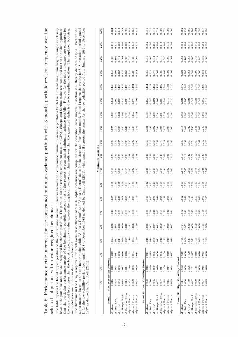
Tab

le6:

Per

form

ance

met

ric

infe

rence

for

the

const

rain

edm

inim

um

-var

iance

por

tfol

ios

wit

h3

mon

ths

por

tfol

iore

vis

ion

freq

uen

cyov

erth

ese

lect

edsu

bp

erio

ds

wit

ha

valu

ew

eigh

ted

ben

chm

ark

Th

eta

ble

rep

ort

sth

eb

oots

trap

ped

p-v

alu

esof

the

per

form

an

cem

etri

cd

iffer

ence

sb

etw

een

the

con

stra

ined

min

imu

m-v

ari

an

cep

ort

folios

(wit

hth

ed

iffer

ent

maxim

um

wei

ght

asi

ngle

stock

may

have

inth

ep

ort

foli

o)

an

dth

evalu

ew

eighte

db

ench

mark

port

folio.

Th

ep

-valu

esfo

rth

ece

rtain

tyeq

uiv

ale

nt

mea

sure

(CE

Q),

Sh

arp

ean

dS

ort

ino

rati

os

are

com

pu

ted

for

the

on

esi

ded

hyp

oth

esis

that

the

part

icu

lar

per

form

an

cem

etri

cof

the

ben

chm

ark

port

foli

oex

ceed

sth

at

of

the

resp

ecti

ve

con

stra

ined

min

imu

m-v

ari

an

cep

ort

folio.

P-v

alu

esfo

rth

ealp

ha

mea

sure

sare

com

pu

ted

for

the

on

esi

ded

hyp

oth

eses

that

the

boots

trap

ped

alp

ha

t-valu

eex

ceed

sth

eem

pir

ical

t-valu

ean

dth

us

ind

icate

sth

at

the

gen

erate

dalp

ha

isd

ue

tosa

mp

lin

gvari

ati

on

.T

he

emp

loyed

boots

trap

met

hod

olo

gie

sare

ou

tlin

ein

det

ail

inse

ctio

n2.3

.T

he

diff

eren

cein

the

CE

Qis

rep

ort

edfo

ra

risk

aver

sion

coeffi

cien

tofγ

=4.

Alp

ha

mea

sure

sare

com

pu

ted

for

the

des

crib

edfa

ctor

mod

els

inse

ctio

n2.2

.H

ereb

yd

enote

s”A

lph

a1

Fact

or”

the

alp

ha

mea

sure

base

don

the

on

efa

ctor

mod

el,

wh

ile

”A

lph

a3

Fact

or”

an

d”A

lph

a4

Fact

or”

do

sofo

rth

eth

ree

and

fou

rfa

ctor

mod

el.

Pan

elI

rep

ort

sth

ere

sult

sfo

rU

.S.

rece

ssio

np

erio

ds,

pan

elII

for

the

low

vola

tility

per

iod

from

Ap

ril

1968

toD

ecem

ber

1985

as

defi

ned

by

Cam

pb

ell

(2001),

wh

ile

pan

elII

Ire

port

sth

ere

sult

sfo

rth

elo

wvola

tility

per

iod

from

Janu

ary

1986

toD

ecem

ber

1997

as

defi

ned

by

Cam

pb

ell

(2001).

Maxim

um

Weig

hts

2%

3%

4%

5%

6%

7%

8%

9%

10%

11%

12%

13%

14%

15%

16%

17%

18%

19%

20%

PanelI:U

.S.R

ecessio

nPerio

ds

∆M

ean

0.0

15

0.0

10

0.0

12

0.0

24

0.0

50

0.0

48

0.0

67

0.0

61

0.1

19

0.1

23

0.1

29

0.1

25

0.1

06

0.1

44

0.1

40

0.1

43

0.0

06

0.1

13

0.1

04

∆Std

.D

ev.

0.8

95

0.9

44

0.9

87

0.9

87

0.9

74

0.8

98

0.9

59

0.7

40

0.6

84

0.5

89

0.5

34

0.7

13

0.2

59

0.1

60

0.1

96

0.1

04

0.1

02

0.1

30

0.1

43

∆C

EQ

0.0

04

0.0

06

0.0

08

0.0

11

0.0

22

0.0

31

0.0

39

0.0

57

0.0

99

0.1

23

0.1

25

0.0

96

0.1

37

0.1

90

0.1

66

0.1

85

0.0

12

0.2

03

0.2

42

∆Sharp

eR

ati

o0.0

18

0.0

17

0.0

16

0.0

29

0.0

60

0.0

57

0.0

78

0.0

69

0.1

24

0.1

27

0.1

30

0.1

40

0.1

07

0.1

36

0.1

32

0.1

37

0.0

08

0.1

03

0.0

88

∆Sort

ino

Rati

o0.0

14

0.0

14

0.0

16

0.0

27

0.0

49

0.0

51

0.0

68

0.0

64

0.1

15

0.1

24

0.1

26

0.1

34

0.0

98

0.1

28

0.1

23

0.1

33

0.0

08

0.1

03

0.0

91

Alp

ha

1Facto

r0.2

23

0.2

19

0.1

92

0.1

89

0.2

32

0.2

27

0.2

96

0.2

42

0.3

60

0.3

58

0.3

52

0.3

26

0.2

87

0.3

31

0.3

25

0.3

24

0.0

26

0.2

28

0.1

89

Alp

ha

3Facto

r0.0

29

0.0

58

0.0

34

0.0

54

0.0

96

0.0

96

0.0

97

0.1

38

0.2

22

0.2

02

0.2

22

0.2

46

0.1

52

0.1

76

0.1

91

0.2

08

0.0

30

0.1

42

0.1

50

Alp

ha

4Facto

r0.0

68

0.0

99

0.0

84

0.1

20

0.1

69

0.1

51

0.1

79

0.2

28

0.3

42

0.3

38

0.3

90

0.3

83

0.2

48

0.2

93

0.3

42

0.3

48

0.0

67

0.2

34

0.2

16

PanelII:Low

Vola

tility

Perio

d

∆M

ean

0.0

08

0.0

13

0.0

11

0.0

15

0.0

53

0.0

51

0.1

01

0.0

32

0.0

36

0.1

29

0.0

59

0.0

81

0.0

88

0.1

50

0.1

51

0.0

50

0.0

16

0.0

82

0.0

10

∆Std

.D

ev.

0.7

10

0.8

20

0.8

85

0.9

14

0.9

02

0.7

96

0.8

67

0.6

53

0.4

72

0.7

59

0.6

12

0.4

99

0.3

82

0.3

45

0.4

28

0.3

14

0.4

05

0.0

95

0.0

16

∆C

EQ

0.0

05

0.0

09

0.0

05

0.0

09

0.0

37

0.0

48

0.0

79

0.0

23

0.0

44

0.1

07

0.0

68

0.0

92

0.1

04

0.1

91

0.1

67

0.0

78

0.0

14

0.1

59

0.0

45

∆Sharp

eR

ati

o0.0

07

0.0

10

0.0

06

0.0

12

0.0

43

0.0

47

0.0

89

0.0

27

0.0

40

0.1

14

0.0

58

0.0

84

0.0

94

0.1

62

0.1

53

0.0

62

0.0

14

0.1

01

0.0

22

∆Sort

ino

Rati

o0.0

07

0.0

11

0.0

05

0.0

12

0.0

50

0.0

51

0.0

98

0.0

29

0.0

48

0.1

43

0.0

76

0.0

94

0.1

20

0.1

86

0.1

92

0.0

86

0.0

16

0.1

14

0.0

20

Alp

ha

1Facto

r0.2

74

0.2

00

0.1

69

0.1

73

0.2

11

0.1

95

0.1

98

0.1

53

0.1

86

0.2

69

0.2

11

0.1

73

0.2

27

0.2

84

0.2

84

0.1

99

0.0

86

0.1

92

0.0

71

Alp

ha

3Facto

r0.0

15

0.0

17

0.0

10

0.0

10

0.0

10

0.0

12

0.0

08

0.0

01

0.0

02

0.0

21

0.0

05

0.0

08

0.0

09

0.0

16

0.0

24

0.0

07

0.0

00

0.0

12

0.0

01

Alp

ha

4Facto

r0.0

35

0.0

24

0.0

17

0.0

15

0.0

17

0.0

11

0.0

11

0.0

03

0.0

03

0.0

13

0.0

09

0.0

06

0.0

04

0.0

20

0.0

20

0.0

03

0.0

04

0.0

01

0.0

00

PanelIII:H

igh

Vola

tility

Perio

d

∆M

ean

0.5

11

0.6

32

0.6

18

0.7

75

0.7

64

0.6

72

0.5

62

0.8

17

0.6

74

0.5

10

0.6

33

0.7

18

0.5

66

0.5

21

0.5

72

0.6

24

0.9

61

0.8

54

0.5

82

∆Std

.D

ev.

1.0

00

1.0

00

1.0

00

1.0

00

0.9

72

0.9

11

0.9

38

0.7

93

0.5

65

0.3

18

0.3

99

0.4

09

0.2

06

0.1

85

0.2

48

0.2

85

0.1

63

0.1

91

0.1

32

∆C

EQ

0.1

89

0.3

28

0.4

20

0.6

17

0.6

32

0.5

90

0.4

56

0.7

56

0.6

61

0.5

42

0.6

60

0.7

22

0.6

38

0.6

21

0.6

30

0.6

64

0.9

66

0.8

78

0.6

86

∆Sharp

eR

ati

o0.0

47

0.1

31

0.3

17

0.5

72

0.6

08

0.5

85

0.4

34

0.7

60

0.6

78

0.5

72

0.6

74

0.7

33

0.6

62

0.6

42

0.6

49

0.6

84

0.9

65

0.8

80

0.7

06

∆Sort

ino

Rati

o0.0

59

0.1

15

0.2

48

0.4

95

0.5

52

0.5

03

0.3

51

0.7

17

0.5

78

0.4

52

0.5

60

0.6

41

0.5

55

0.5

31

0.5

73

0.5

99

0.9

48

0.8

42

0.6

04

Alp

ha

1Facto

r0.0

00

0.0

00

0.0

10

0.0

33

0.0

66

0.0

45

0.0

30

0.1

34

0.0

74

0.0

38

0.0

67

0.1

02

0.0

43

0.0

47

0.0

49

0.0

60

0.4

40

0.1

87

0.0

36

Alp

ha

3Facto

r0.0

07

0.0

18

0.0

33

0.1

27

0.1

53

0.1

69

0.0

73

0.3

66

0.2

28

0.1

40

0.2

12

0.2

40

0.1

63

0.1

52

0.1

27

0.1

33

0.6

36

0.2

84

0.1

17

Alp

ha

4Facto

r0.0

43

0.0

46

0.0

80

0.2

99

0.3

50

0.4

38

0.2

87

0.7

14

0.5

57

0.2

97

0.4

26

0.3

31

0.3

64

0.3

19

0.2

80

0.2

72

0.6

03

0.3

35

0.2

51

31

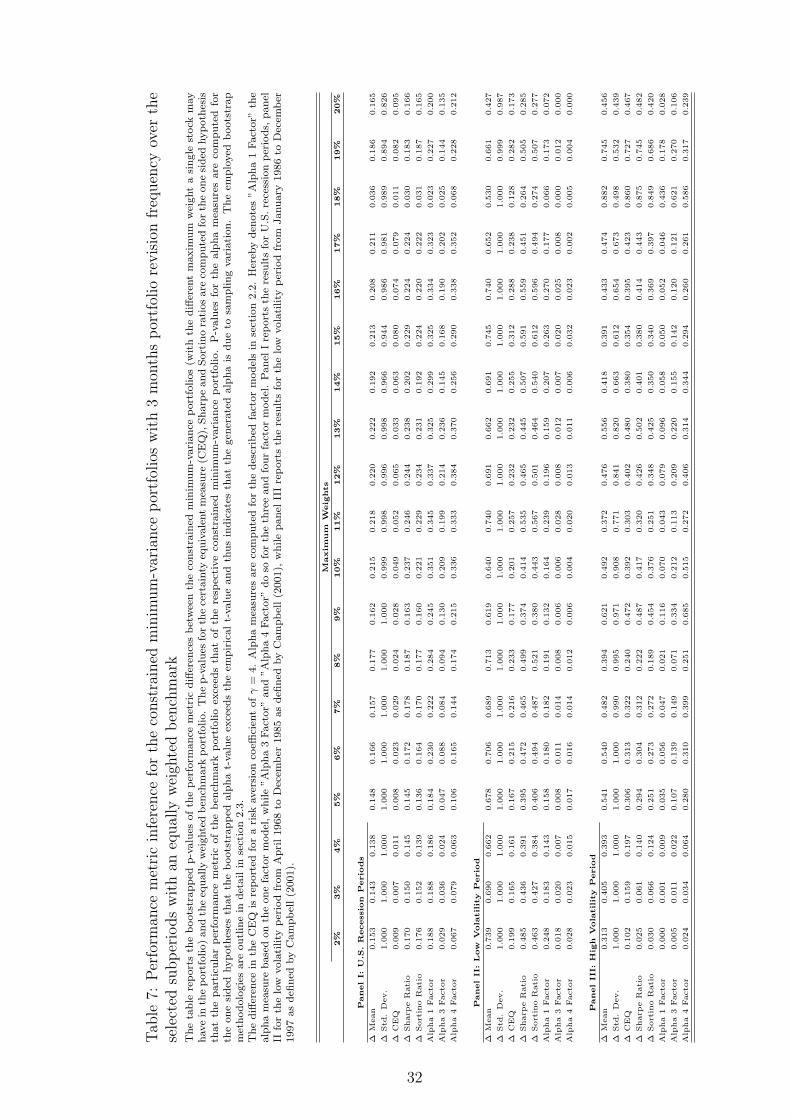
Tab

le7:

Per

form

ance

met

ric

infe

rence

for

the

const

rain

edm

inim

um

-var

iance

por

tfol

ios

wit

h3

mon

ths

por

tfol

iore

vis

ion

freq

uen

cyov

erth

ese

lect

edsu

bp

erio

ds

wit

han

equal

lyw

eigh

ted

ben

chm

ark

Th

eta

ble

rep

ort

sth

eb

oots

trap

ped

p-v

alu

esof

the

per

form

an

cem

etri

cd

iffer

ence

sb

etw

een

the

con

stra

ined

min

imu

m-v

ari

an

cep

ort

folios

(wit

hth

ed

iffer

ent

maxim

um

wei

ght

asi

ngle

stock

may

have

inth

ep

ort

folio)

an

dth

eeq

ually

wei

ghte

db

ench

mark

port

folio.

Th

ep

-valu

esfo

rth

ece

rtain

tyeq

uiv

ale

nt

mea

sure

(CE

Q),

Sh

arp

ean

dS

ort

ino

rati

os

are

com

pu

ted

for

the

on

esi

ded

hyp

oth

esis

that

the

part

icu

lar

per

form

an

cem

etri

cof

the

ben

chm

ark

port

foli

oex

ceed

sth

at

of

the

resp

ecti

ve

con

stra

ined

min

imu

m-v

ari

an

cep

ort

folio.

P-v

alu

esfo

rth

ealp

ha

mea

sure

sare

com

pu

ted

for

the

on

esi

ded

hyp

oth

eses

that

the

boots

trap

ped

alp

ha

t-valu

eex

ceed

sth

eem

pir

ical

t-valu

ean

dth

us

ind

icate

sth

at

the

gen

erate

dalp

ha

isd

ue

tosa

mp

lin

gvari

ati

on

.T

he

emp

loyed

boots

trap

met

hod

olo

gie

sare

ou

tlin

ein

det

ail

inse

ctio

n2.3

.T

he

diff

eren

cein

the

CE

Qis

rep

ort

edfo

ra

risk

aver

sion

coeffi

cien

tofγ

=4.

Alp

ha

mea

sure

sare

com

pu

ted

for

the

des

crib

edfa

ctor

mod

els

inse

ctio

n2.2

.H

ereb

yd

enote

s”A

lph

a1

Fact

or”

the

alp

ha

mea

sure

base

don

the

on

efa

ctor

mod

el,

wh

ile

”A

lph

a3

Fact

or”

an

d”A

lph

a4

Fact

or”

do

sofo

rth

eth

ree

and

fou

rfa

ctor

mod

el.

Pan

elI

rep

ort

sth

ere

sult

sfo

rU

.S.

rece

ssio

np

erio

ds,

pan

elII

for

the

low

vola

tility

per

iod

from

Ap

ril

1968

toD

ecem

ber

1985

as

defi

ned

by

Cam

pb

ell

(2001),

wh

ile

pan

elII

Ire

port

sth

ere

sult

sfo

rth

elo

wvola

tility

per

iod

from

Janu

ary

1986

toD

ecem

ber

1997

as

defi

ned

by

Cam

pb

ell

(2001).

Maxim

um

Weig

hts

2%

3%

4%

5%

6%

7%

8%

9%

10%

11%

12%

13%

14%

15%

16%

17%

18%

19%

20%

PanelI:U

.S.R

ecessio

nPerio

ds

∆M

ean

0.1

53

0.1

43

0.1

38

0.1

48

0.1

66

0.1

57

0.1

77

0.1

62

0.2

15

0.2

18

0.2

20

0.2

22

0.1

92

0.2

13

0.2

08

0.2

11

0.0

36

0.1

86

0.1

65

∆Std

.D

ev.

1.0

00

1.0

00

1.0

00

1.0

00

1.0

00

1.0

00

1.0

00

1.0

00

0.9

99

0.9

98

0.9

96

0.9

98

0.9

66

0.9

44

0.9

86

0.9

81

0.9

89

0.8

94

0.8

26

∆C

EQ

0.0

09

0.0

07

0.0

11

0.0

08

0.0

23

0.0

29

0.0

24

0.0

28

0.0

49

0.0

52

0.0

65

0.0

33

0.0

63

0.0

80

0.0

74

0.0

79

0.0

11

0.0

82

0.0

95

∆Sharp

eR

ati

o0.1

70

0.1

50

0.1

45

0.1

45

0.1

72

0.1

78

0.1

87

0.1

63

0.2

37

0.2

46

0.2

44

0.2

38

0.2

02

0.2

29

0.2

24

0.2

24

0.0

30

0.1

83

0.1

66

∆Sort

ino

Rati

o0.1

76

0.1

52

0.1

39

0.1

36

0.1

64

0.1

70

0.1

77

0.1

60

0.2

21

0.2

29

0.2

34

0.2

31

0.1

92

0.2

24

0.2

20

0.2

22

0.0

31

0.1

87

0.1

65

Alp

ha

1Facto

r0.1

88

0.1

88

0.1

86

0.1

84

0.2

30

0.2

22

0.2

84

0.2

45

0.3

51

0.3

45

0.3

37

0.3

25

0.2

99

0.3

25

0.3

34

0.3

23

0.0

23

0.2

27

0.2

00

Alp

ha

3Facto

r0.0

29

0.0

36

0.0

24

0.0

47

0.0

88

0.0

84

0.0

94

0.1

30

0.2

09

0.1

99

0.2

14

0.2

36

0.1

45

0.1

68

0.1

90

0.2

02

0.0

25

0.1

44

0.1

35

Alp

ha

4Facto

r0.0

67

0.0

79

0.0

63

0.1

06

0.1

65

0.1

44

0.1

74

0.2

15

0.3

36

0.3

33

0.3

84

0.3

70

0.2

56

0.2

90

0.3

38

0.3

52

0.0

68

0.2

28

0.2

12

PanelII:Low

Vola

tility

Perio

d

∆M

ean

0.7

39

0.6

90

0.6

62

0.6

78

0.7

06

0.6

89

0.7

13

0.6

19

0.6

40

0.7

40

0.6

91

0.6

62

0.6

91

0.7

45

0.7

40

0.6

52

0.5

30

0.6

61

0.4

27

∆Std

.D

ev.

1.0

00

1.0

00

1.0

00

1.0

00

1.0

00

1.0

00

1.0

00

1.0

00

1.0

00

1.0

00

1.0

00

1.0

00

1.0

00

1.0

00

1.0

00

1.0

00

1.0

00

0.9

99

0.9

87

∆C

EQ

0.1

99

0.1

65

0.1

61

0.1

67

0.2

15

0.2

16

0.2

33

0.1

77

0.2

01

0.2

57

0.2

32

0.2

32

0.2

55

0.3

12

0.2

88

0.2

38

0.1

28

0.2

82

0.1

73

∆Sharp

eR

ati

o0.4

85

0.4

36

0.3

91

0.3

95

0.4

72

0.4

65

0.4

99

0.3

74

0.4

14

0.5

35

0.4

65

0.4

45

0.5

07

0.5

91

0.5

59

0.4

51

0.2

64

0.5

05

0.2

85

∆Sort

ino

Rati

o0.4

63

0.4

27

0.3

84

0.4

06

0.4

94

0.4

87

0.5

21

0.3

80

0.4

43

0.5

67

0.5

01

0.4

64

0.5

40

0.6

12

0.5

96

0.4

94

0.2

74

0.5

07

0.2

77

Alp

ha

1Facto

r0.2

48

0.1

83

0.1

43

0.1

58

0.1

80

0.1

82

0.1

91

0.1

32

0.1

64

0.2

39

0.1

96

0.1

59

0.2

07

0.2

63

0.2

70

0.1

77

0.0

66

0.1

73

0.0

72

Alp

ha

3Facto

r0.0

18

0.0

20

0.0

07

0.0

08

0.0

11

0.0

14

0.0

08

0.0

06

0.0

06

0.0

28

0.0

08

0.0

12

0.0

07

0.0

20

0.0

25

0.0

08

0.0

00

0.0

12

0.0

00

Alp

ha

4Facto

r0.0

28

0.0

23

0.0

15

0.0

17

0.0

16

0.0

14

0.0

12

0.0

06

0.0

04

0.0

20

0.0

13

0.0

11

0.0

06

0.0

32

0.0

23

0.0

02

0.0

05

0.0

04

0.0

00

PanelIII:H

igh

Vola

tility

Perio

d

∆M

ean

0.3

13

0.4

05

0.3

93

0.5

41

0.5

40

0.4

82

0.3

94

0.6

21

0.4

92

0.3

72

0.4

76

0.5

56

0.4

18

0.3

91

0.4

33

0.4

74

0.8

82

0.7

45

0.4

56

∆Std

.D

ev.

1.0

00

1.0

00

1.0

00

1.0

00

1.0

00

0.9

90

0.9

95

0.9

71

0.9

08

0.7

71

0.8

41

0.8

20

0.6

63

0.6

12

0.6

54

0.6

73

0.4

98

0.5

32

0.4

39

∆C

EQ

0.1

02

0.1

59

0.1

97

0.3

06

0.3

13

0.3

22

0.2

40

0.4

72

0.3

92

0.3

03

0.4

02

0.4

80

0.3

80

0.3

54

0.3

95

0.4

23

0.8

60

0.7

27

0.4

67

∆Sharp

eR

ati

o0.0

25

0.0

61

0.1

40

0.2

94

0.3

04

0.3

12

0.2

22

0.4

87

0.4

17

0.3

20

0.4

26

0.5

02

0.4

01

0.3

80

0.4

14

0.4

43

0.8

75

0.7

45

0.4

82

∆Sort

ino

Rati

o0.0

30

0.0

66

0.1

24

0.2

51

0.2

73

0.2

72

0.1

89

0.4

54

0.3

76

0.2

51

0.3

48

0.4

25

0.3

50

0.3

40

0.3

69

0.3

97

0.8

49

0.6

86

0.4

20

Alp

ha

1Facto

r0.0

00

0.0

01

0.0

09

0.0

35

0.0

56

0.0

47

0.0

21

0.1

16

0.0

70

0.0

43

0.0

79

0.0

96

0.0

58

0.0

50

0.0

52

0.0

46

0.4

36

0.1

78

0.0

28

Alp

ha

3Facto

r0.0

05

0.0

11

0.0

22

0.1

07

0.1

39

0.1

49

0.0

71

0.3

34

0.2

12

0.1

13

0.2

09

0.2

20

0.1

55

0.1

42

0.1

20

0.1

21

0.6

21

0.2

70

0.1

06

Alp

ha

4Facto

r0.0

24

0.0

34

0.0

64

0.2

80

0.3

10

0.3

99

0.2

51

0.6

85

0.5

15

0.2

72

0.4

06

0.3

14

0.3

44

0.2

94

0.2

60

0.2

61

0.5

86

0.3

17

0.2

39

32

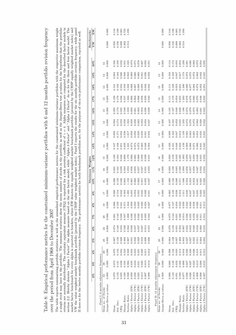
Tab

le8:

Em

pir

ical

per

form

ance

met

rics

for

the

const

rain

edm

inim

um

-var

iance

por

tfol

ios

wit

h6

and

12m

onth

sp

ortf

olio

revis

ion

freq

uen

cyov

erth

ep

erio

dfr

omA

pri

l19

68to

Dec

emb

er20

07T

he

tab

lere

port

ssu

mm

ari

zin

gp

ort

folio

stati

stic

sas

wel

las

the

an

nu

alize

dem

pir

ical

per

form

an

cem

etri

csfo

rth

eco

nst

rain

edm

inim

um

-vari

an

cep

ort

folios

wit

hth

ere

spec

tive

maxim

um

wei

ght

asi

ngle

stock

may

have

inth

ep

ort

folio.

Th

esu

mm

ary

stati

stic

ssh

ow

the

mea

nnum

ber

of

stock

sin

the

port

foli

oas

wel

las

the

Jarq

ue-

Ber

rate

stp

-valu

esfo

rth

ehyp

oth

esis

that

the

port

folio

retu

rns

are

norm

ally

dis

trib

ute

d.

Th

ece

rtain

tyeq

uiv

ale

nt

mea

sure

(CE

Q)

isre

port

edfo

ra

risk

aver

sion

coeffi

cien

tofγ

=4.

Alp

ha

mea

sure

sare

com

pu

ted

for

the

des

crib

edfa

ctor

mod

els

inse

ctio

n2.2

.H

ereb

yd

enote

s”A

lph

a1

Fact

or”

the

alp

ha

mea

sure

base

don

the

on

efa

ctor

mod

el,

wh

ile

”A

lph

a3

Fact

or”

an

d”A

lph

a4

Fact

or”

do

sofo

rth

eth

ree

an

dfo

ur

fact

or

mod

el.

Th

em

ark

etfa

ctor

ben

chm

ark

for

ever

yalp

ha

isre

port

edin

bra

cket

s,w

her

eE

Wd

enote

sth

eeq

ually

wei

ghte

dm

ark

etb

ench

mark

port

folio

(pro

xie

dby

the

CR

SP

equ

ally

wei

ghte

dm

ark

etin

dex

)an

dV

Wth

evalu

ew

eighte

dm

ark

etb

ench

mark

port

folio

(pro

xie

dby

the

CR

SP

valu

ew

eighte

dm

ark

etin

dex

).P

an

elI

rep

ort

sth

ere

sult

sfo

rth

esi

xm

onth

sp

ort

folio

revis

ion

freq

uen

cy,

wh

ile

pan

elII

does

sofo

rth

etw

elve

month

sp

ort

foli

ore

vis

ion

freq

uen

cy.

Th

ep

erfo

rman

cem

etri

csfo

rb

oth

ben

chm

ark

port

folios

are

,fo

rth

epu

rpose

of

vis

-a-v

isp

erfo

rman

ceco

mp

ari

son

,re

port

edas

wel

l.

Maxim

um

Weig

hts

Benchm

arks

2%

3%

4%

5%

6%

7%

8%

9%

10%

11%

12%

13%

14%

15%

16%

17%

18%

19%

20%

VW

EW

Panel

I:6

month

sadju

stm

ent

frequency

Mean

no.

of

Sto

cks

53

38

29

25

22

20

18

17

16

16

15

14

14

14

13

13

12

12

12

Jarq

ue-B

err

ap-v

alu

es

0.0

00

0.0

00

0.0

00

0.0

00

0.0

00

0.0

00

0.0

00

0.0

00

0.0

00

0.0

00

0.0

00

0.0

00

0.0

00

0.0

00

0.0

00

0.0

00

0.0

00

0.0

00

0.0

00

0.0

00

0.0

00

Mean

0.0

70

0.0

72

0.0

70

0.0

67

0.0

74

0.0

81

0.0

86

0.0

90

0.0

96

0.0

91

0.1

00

0.1

07

0.0

92

0.0

94

0.0

95

0.1

00

0.1

01

0.0

94

0.1

06

0.0

56

0.1

44

Std

.D

ev.

0.1

32

0.1

31

0.1

34

0.1

39

0.1

40

0.1

45

0.1

50

0.1

54

0.1

59

0.1

61

0.1

64

0.1

68

0.1

71

0.1

74

0.1

74

0.1

79

0.1

83

0.1

84

0.1

93

0.1

56

0.1

98

CE

Q0.0

35

0.0

38

0.0

34

0.0

28

0.0

34

0.0

39

0.0

41

0.0

42

0.0

46

0.0

39

0.0

46

0.0

51

0.0

34

0.0

33

0.0

35

0.0

36

0.0

34

0.0

26

0.0

32

0.0

08

0.0

65

Sharp

eR

ati

o0.5

30

0.5

55

0.5

23

0.4

82

0.5

26

0.5

57

0.5

71

0.5

83

0.6

05

0.5

63

0.6

09

0.6

39

0.5

38

0.5

39

0.5

48

0.5

57

0.5

50

0.5

09

0.5

51

0.3

62

0.7

25

Sort

ino

Rati

o0.9

29

0.9

84

0.9

49

0.8

67

0.9

44

1.0

06

1.0

44

1.0

85

1.1

32

1.0

53

1.1

70

1.2

21

1.0

17

1.0

24

1.0

33

1.0

44

1.0

22

0.9

43

1.0

25

0.5

14

1.0

56

Alp

ha

1Facto

r(E

W)

0.0

30

0.0

35

0.0

34

0.0

31

0.0

38

0.0

46

0.0

50

0.0

55

0.0

61

0.0

56

0.0

66

0.0

74

0.0

58

0.0

59

0.0

62

0.0

66

0.0

68

0.0

60

0.0

74

Alp

ha

1Facto

r(V

W)

0.0

30

0.0

34

0.0

33

0.0

30

0.0

37

0.0

45

0.0

50

0.0

54

0.0

60

0.0

55

0.0

65

0.0

74

0.0

56

0.0

58

0.0

61

0.0

64

0.0

67

0.0

60

0.0

71

Alp

ha

3Facto

r(E

W)

0.0

25

0.0

31

0.0

31

0.0

29

0.0

37

0.0

46

0.0

49

0.0

55

0.0

62

0.0

57

0.0

68

0.0

73

0.0

59

0.0

62

0.0

63

0.0

68

0.0

69

0.0

60

0.0

78

Alp

ha

3Facto

r(V

W)

0.0

13

0.0

20

0.0

20

0.0

18

0.0

27

0.0

35

0.0

40

0.0

45

0.0

51

0.0

47

0.0

58

0.0

65

0.0

50

0.0

52

0.0

54

0.0

58

0.0

59

0.0

51

0.0

67

Alp

ha

4Facto

r(E

W)

0.0

07

0.0

13

0.0

11

0.0

06

0.0

14

0.0

23

0.0

24

0.0

29

0.0

35

0.0

31

0.0

38

0.0

48

0.0

31

0.0

34

0.0

36

0.0

39

0.0

42

0.0

36

0.0

50

Alp

ha

4Facto

r(V

W)

0.0

08

0.0

14

0.0

12

0.0

06

0.0

15

0.0

24

0.0

27

0.0

31

0.0

37

0.0

33

0.0

41

0.0

52

0.0

34

0.0

37

0.0

39

0.0

42

0.0

44

0.0

39

0.0

51

Panel

II:

12

month

sadju

stm

ent

frequency

Mean

no.

of

Sto

cks

53

38

30

25

23

21

18

17

17

16

16

13

15

15

14

13

12

13

12

Jarq

ue-B

err

ap-v

alu

es

0.0

00

0.0

00

0.0

00

0.0

00

0.0

00

0.0

00

0.0

00

0.0

00

0.0

00

0.0

00

0.0

00

0.0

00

0.0

00

0.0

00

0.0

00

0.0

00

0.0

00

0.0

00

0.0

00

0.0

00

0.0

00

Mean

0.0

66

0.0

66

0.0

68

0.0

64

0.0

70

0.0

73

0.0

77

0.0

83

0.0

89

0.0

93

0.0

93

0.1

00

0.0

99

0.1

07

0.1

05

0.1

11

0.1

11

0.1

04

0.1

14

0.0

56

0.1

44

Std

.D

ev.

0.1

33

0.1

30

0.1

32

0.1

38

0.1

39

0.1

44

0.1

47

0.1

50

0.1

56

0.1

58

0.1

58

0.1

61

0.1

62

0.1

65

0.1

67

0.1

70

0.1

69

0.1

69

0.1

74

0.1

56

0.1

98

CE

Q0.0

31

0.0

32

0.0

33

0.0

27

0.0

31

0.0

31

0.0

34

0.0

38

0.0

40

0.0

43

0.0

43

0.0

48

0.0

47

0.0

52

0.0

49

0.0

54

0.0

53

0.0

47

0.0

53

0.0

08

0.0

65

Sharp

eR

ati

o0.5

00

0.5

09

0.5

13

0.4

69

0.5

03

0.5

06

0.5

22

0.5

54

0.5

71

0.5

89

0.5

85

0.6

22

0.6

12

0.6

45

0.6

29

0.6

55

0.6

54

0.6

17

0.6

54

0.3

62

0.7

25

Sort

ino

Rati

o0.8

77

0.8

88

0.9

16

0.8

43

0.9

07

0.9

14

0.9

30

1.0

11

1.0

46

1.0

94

1.0

93

1.1

39

1.1

49

1.2

35

1.1

90

1.2

43

1.2

40

1.1

74

1.2

30

0.5

14

1.0

56

Alp

ha

1Facto

r(E

W)

0.0

26

0.0

27

0.0

30

0.0

27

0.0

34

0.0

36

0.0

42

0.0

49

0.0

54

0.0

58

0.0

59

0.0

69

0.0

65

0.0

72

0.0

72

0.0

78

0.0

80

0.0

72

0.0

81

Alp

ha

1Facto

r(V

W)

0.0

26

0.0

27

0.0

30

0.0

27

0.0

33

0.0

35

0.0

40

0.0

47

0.0

53

0.0

57

0.0

57

0.0

66

0.0

63

0.0

70

0.0

70

0.0

76

0.0

77

0.0

70

0.0

80

Alp

ha

3Facto

r(E

W)

0.0

19

0.0

23

0.0

26

0.0

23

0.0

29

0.0

32

0.0

38

0.0

47

0.0

52

0.0

58

0.0

59

0.0

71

0.0

65

0.0

72

0.0

73

0.0

80

0.0

82

0.0

72

0.0

82

Alp

ha

3Facto

r(V

W)

0.0

08

0.0

13

0.0

15

0.0

11

0.0

18

0.0

21

0.0

26

0.0

35

0.0

41

0.0

47

0.0

48

0.0

60

0.0

54

0.0

62

0.0

63

0.0

70

0.0

72

0.0

62

0.0

72

Alp

ha

4Facto

r(E

W)

0.0

06

0.0

08

0.0

11

0.0

04

0.0

09

0.0

11

0.0

11

0.0

22

0.0

25

0.0

32

0.0

31

0.0

41

0.0

33

0.0

39

0.0

41

0.0

48

0.0

52

0.0

42

0.0

54

Alp

ha

4Facto

r(V

W)

0.0

07

0.0

10

0.0

12

0.0

04

0.0

10

0.0

12

0.0

13

0.0

23

0.0

26

0.0

34

0.0

32

0.0

40

0.0

35

0.0

42

0.0

43

0.0

50

0.0

54

0.0

45

0.0

56

33

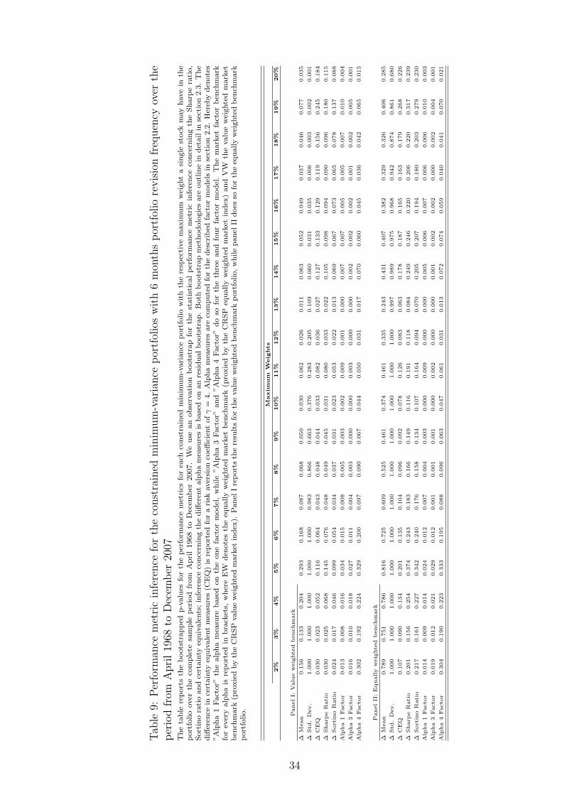
Tab

le9:

Per

form

ance

met

ric

infe

rence

for

the

const

rain

edm

inim

um

-var

iance

por

tfol

ios

wit

h6

mon

ths

por

tfol

iore

vis

ion

freq

uen

cyov

erth

ep

erio

dfr

omA

pri

l19

68to

Dec

emb

er20

07T

he

tab

lere

port

sth

eb

oots

trap

ped

p-v

alu

esfo

rth

ep

erfo

rman

cem

etri

csfo

rea

chco

nst

rain

edm

inim

um

-vari

an

cep

ort

folio

wit

hth

ere

spec

tive

maxim

um

wei

ght

asi

ngle

stock

may

have

inth

ep

ort

folio

over

the

com

ple

tesa

mp

lep

erio

dfr

om

Ap

ril

1968

toD

ecem

ber

2007.

We

use

an

ob

serv

ati

on

boots

trap

for

the

stati

stic

al

per

form

an

cem

etri

cin

fere

nce

con

cern

ing

the

Sh

arp

era

tio,

Sort

ino

rati

oan

dce

rtain

tyeq

uiv

ale

nts

;in

fere

nce

con

cern

ing

the

diff

eren

talp

ha

mea

sure

sis

base

don

an

resi

du

al

boots

trap

.B

oth

boots

trap

met

hod

olo

gie

sare

ou

tlin

ein

det

ail

inse

ctio

n2.3

.T

he

diff

eren

cein

cert

ain

tyeq

uiv

ale

nt

mea

sure

s(C

EQ

)is

rep

ort

edfo

ra

risk

aver

sion

coeffi

cien

tofγ

=4.

Alp

ha

mea

sure

sare

com

pu

ted

for

the

des

crib

edfa

ctor

mod

els

inse

ctio

n2.2

.H

ereb

yd

enote

s”A

lph

a1

Fact

or”

the

alp

ha

mea

sure

base

don

the

on

efa

ctor

mod

el,

wh

ile

”A

lph

a3

Fact

or”

an

d”A

lph

a4

Fact

or”

do

sofo

rth

eth

ree

an

dfo

ur

fact

or

mod

el.

Th

em

ark

etfa

ctor

ben

chm

ark

for

ever

yalp

ha

isre

port

edin

bra

cket

s,w

her

eE

Wd

enote

sth

eeq

ually

wei

ghte

dm

ark

etb

ench

mark

(pro

xie

dby

the

CR

SP

equ

all

yw

eighte

dm

ark

etin

dex

)an

dV

Wth

evalu

ew

eighte

dm

ark

etb

ench

mark

(pro

xie

dby

the

CR

SP

valu

ew

eighte

dm

ark

etin

dex

).P

an

elI

rep

ort

sth

ere

sult

sfo

rth

evalu

ew

eighte

db

ench

mark

port

folio,

wh

ile

pan

elII

does

sofo

rth

eeq

ually

wei

ghte

db

ench

mark

port

folio.

Maxim

um

Weig

hts

2%

3%

4%

5%

6%

7%

8%

9%

10%

11%

12%

13%

14%

15%

16%

17%

18%

19%

20%

Panel

I:V

alu

ew

eig

hte

db

enchm

ark

∆M

ean

0.1

56

0.1

33

0.2

04

0.2

93

0.1

68

0.0

87

0.0

68

0.0

50

0.0

30

0.0

62

0.0

26

0.0

11

0.0

63

0.0

52

0.0

49

0.0

37

0.0

46

0.0

77

0.0

35

∆Std

.D

ev.

1.0

00

1.0

00

1.0

00

1.0

00

1.0

00

0.9

83

0.8

66

0.6

63

0.3

76

0.2

83

0.2

05

0.1

09

0.0

60

0.0

31

0.0

35

0.0

06

0.0

03

0.0

02

0.0

01

∆C

EQ

0.0

30

0.0

23

0.0

52

0.1

16

0.0

64

0.0

43

0.0

48

0.0

44

0.0

33

0.0

82

0.0

36

0.0

27

0.1

27

0.1

33

0.1

29

0.1

19

0.1

56

0.2

45

0.1

84

∆Sharp

eR

ati

o0.0

30

0.0

25

0.0

68

0.1

45

0.0

76

0.0

48

0.0

49

0.0

45

0.0

31

0.0

80

0.0

33

0.0

22

0.1

05

0.0

98

0.0

94

0.0

90

0.0

96

0.1

80

0.1

15

∆Sort

ino

Rati

o0.0

24

0.0

17

0.0

46

0.0

99

0.0

54

0.0

34

0.0

37

0.0

31

0.0

23

0.0

53

0.0

22

0.0

13

0.0

69

0.0

67

0.0

73

0.0

65

0.0

78

0.1

37

0.0

88

Alp

ha

1Facto

r0.0

13

0.0

08

0.0

16

0.0

34

0.0

15

0.0

08

0.0

05

0.0

03

0.0

02

0.0

09

0.0

01

0.0

00

0.0

07

0.0

07

0.0

05

0.0

05

0.0

07

0.0

10

0.0

04

Alp

ha

3Facto

r0.0

16

0.0

10

0.0

18

0.0

27

0.0

11

0.0

04

0.0

03

0.0

00

0.0

00

0.0

03

0.0

00

0.0

00

0.0

02

0.0

02

0.0

02

0.0

01

0.0

02

0.0

05

0.0

01

Alp

ha

4Facto

r0.3

02

0.1

92

0.2

24

0.3

29

0.2

00

0.0

97

0.0

90

0.0

67

0.0

44

0.0

50

0.0

31

0.0

17

0.0

70

0.0

60

0.0

45

0.0

36

0.0

42

0.0

65

0.0

15

Panel

II:

Equall

yw

eig

hte

db

enchm

ark

∆M

ean

0.7

89

0.7

51

0.7

86

0.8

16

0.7

25

0.6

09

0.5

25

0.4

61

0.3

74

0.4

61

0.3

35

0.2

43

0.4

31

0.4

07

0.3

82

0.3

29

0.3

26

0.4

06

0.2

85

∆Std

.D

ev.

1.0

00

1.0

00

1.0

00

1.0

00

1.0

00

1.0

00

1.0

00

1.0

00

1.0

00

1.0

00

1.0

00

0.9

97

0.9

89

0.9

75

0.9

68

0.9

42

0.8

74

0.8

61

0.6

80

∆C

EQ

0.1

07

0.0

90

0.1

34

0.2

01

0.1

35

0.1

04

0.0

96

0.0

92

0.0

78

0.1

26

0.0

83

0.0

63

0.1

78

0.1

87

0.1

65

0.1

63

0.1

79

0.2

68

0.2

26

∆Sharp

eR

ati

o0.2

01

0.1

56

0.2

54

0.3

74

0.2

43

0.1

83

0.1

66

0.1

49

0.1

16

0.1

91

0.1

18

0.0

84

0.2

49

0.2

46

0.2

20

0.2

06

0.2

20

0.3

17

0.2

39

∆Sort

ino

Rati

o0.2

17

0.1

61

0.2

27

0.3

42

0.2

40

0.1

76

0.1

58

0.1

34

0.1

07

0.1

64

0.0

94

0.0

70

0.2

05

0.2

07

0.1

94

0.1

80

0.2

03

0.2

79

0.2

30

Alp

ha

1Facto

r0.0

14

0.0

09

0.0

14

0.0

24

0.0

12

0.0

07

0.0

04

0.0

03

0.0

00

0.0

09

0.0

00

0.0

00

0.0

05

0.0

06

0.0

07

0.0

06

0.0

06

0.0

10

0.0

03

Alp

ha

3Facto

r0.0

19

0.0

12

0.0

21

0.0

29

0.0

12

0.0

01

0.0

01

0.0

01

0.0

00

0.0

02

0.0

00

0.0

00

0.0

01

0.0

02

0.0

02

0.0

00

0.0

02

0.0

04

0.0

01

Alp

ha

4Facto

r0.3

04

0.1

90

0.2

23

0.3

33

0.1

95

0.0

88

0.0

96

0.0

63

0.0

47

0.0

61

0.0

31

0.0

13

0.0

72

0.0

74

0.0

59

0.0

40

0.0

41

0.0

70

0.0

21

34

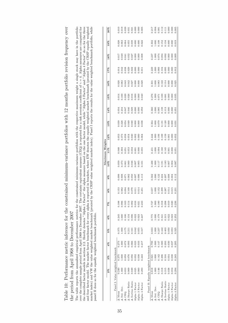
Tab

le10

:P

erfo

rman

cem

etri

cin

fere

nce

for

the

const

rain

edm

inim

um

-var

iance

por

tfol

ios

wit

h12

mon

ths

por

tfol

iore

vis

ion

freq

uen

cyov

erth

ep

erio

dfr

omA

pri

l19

68to

Dec

emb

er20

07T

he

tab

lere

port

sth

ean

nu

alize

dem

pir

ical

per

form

an

cem

etri

csfo

rth

eco

nst

rain

edm

inim

um

-vari

an

cep

ort

folios

wit

hth

ere

spec

tive

maxim

um

wei

ght

asi

ngle

stock

may

have

inth

ep

ort

folio

over

the

com

ple

tesa

mp

lep

erio

dfr

om

Ap

ril

1968

toD

ecem

ber

2007.

The

cert

ain

tyeq

uiv

ale

nt

mea

sure

(CE

Q)

isre

port

edfo

ra

risk

aver

sion

coeffi

cien

tofγ

=4.

Alp

ha

mea

sure

sare

com

pu

ted

for

the

des

crib

edfa

ctor

mod

els

inse

ctio

n2.2

.H

ereb

yd

enote

s”A

lph

a1

Fact

or”

the

alp

ha

mea

sure

base

don

the

one

fact

or

mod

el,

wh

ile

”A

lph

a3

Fact

or”

an

d”A

lpha

4F

act

or”

do

sofo

rth

eth

ree

an

dfo

ur

fact

or

mod

el.

Th

em

ark

etfa

ctor

ben

chm

ark

for

ever

yalp

ha

isre

port

edin

bra

cket

s,w

her

eE

Wd

enote

sth

eeq

ually

wei

ghte

dm

ark

etb

ench

mark

(pro

xie

dby

the

CR

SP

equ

ally

wei

ghte

dm

ark

etin

dex

)an

dV

Wth

evalu

ew

eighte

dm

ark

etb

ench

mark

(pro

xie

dby

the

CR

SP

valu

ew

eighte

dm

ark

etin

dex

).P

an

elI

rep

ort

sth

ere

sult

sfo

rth

evalu

ew

eighte

db

ench

mark

port

folio,

wh

ile

pan

elII

does

sofo

rth

eeq

ually

wei

ghte

db

ench

mark

port

folio.

Maxim

um

Weig

hts

2%

3%

4%

5%

6%

7%

8%

9%

10%

11%

12%

13%

14%

15%

16%

17%

18%

19%

20%

Panel

I:V

alu

ew

eig

hte

db

enchm

ark

∆M

ean

0.2

40

0.2

75

0.2

73

0.3

75

0.2

45

0.1

88

0.1

53

0.0

99

0.0

59

0.0

48

0.0

53

0.0

39

0.0

34

0.0

14

0.0

20

0.0

14

0.0

17

0.0

28

0.0

10

∆Std

.D

ev.

1.0

00

1.0

00

1.0

00

1.0

00

1.0

00

0.9

96

0.9

82

0.9

08

0.4

73

0.3

94

0.3

73

0.2

28

0.2

34

0.1

00

0.0

83

0.0

42

0.0

49

0.0

63

0.0

19

∆C

EQ

0.0

53

0.0

59

0.0

72

0.1

75

0.1

00

0.1

03

0.0

94

0.0

71

0.0

61

0.0

51

0.0

58

0.0

54

0.0

47

0.0

29

0.0

43

0.0

38

0.0

41

0.0

64

0.0

39

∆Sharp

eR

ati

o0.0

69

0.0

76

0.0

93

0.2

11

0.1

34

0.1

14

0.1

09

0.0

82

0.0

60

0.0

53

0.0

54

0.0

49

0.0

46

0.0

26

0.0

42

0.0

29

0.0

32

0.0

55

0.0

31

∆Sort

ino

Rati

o0.0

49

0.0

56

0.0

66

0.1

61

0.0

96

0.0

82

0.0

78

0.0

50

0.0

46

0.0

34

0.0

40

0.0

40

0.0

29

0.0

16

0.0

27

0.0

22

0.0

27

0.0

39

0.0

21

Alp

ha

1Facto

r0.0

25

0.0

32

0.0

23

0.0

42

0.0

22

0.0

16

0.0

11

0.0

07

0.0

07

0.0

01

0.0

02

0.0

00

0.0

00

0.0

00

0.0

00

0.0

00

0.0

00

0.0

00

0.0

00

Alp

ha

3Facto

r0.0

60

0.0

38

0.0

33

0.0

55

0.0

23

0.0

21

0.0

14

0.0

06

0.0

05

0.0

00

0.0

00

0.0

00

0.0

00

0.0

00

0.0

00

0.0

00

0.0

00

0.0

00

0.0

00

Alp

ha

4Facto

r0.2

93

0.2

43

0.2

17

0.3

17

0.2

47

0.2

33

0.2

51

0.1

13

0.1

01

0.0

55

0.0

64

0.0

38

0.0

59

0.0

40

0.0

29

0.0

11

0.0

08

0.0

22

0.0

05

Panel

II:

Equall

yw

eig

hte

db

enchm

ark

∆M

ean

0.8

18

0.8

21

0.7

99

0.8

33

0.7

75

0.7

27

0.6

57

0.5

82

0.4

88

0.4

31

0.4

44

0.3

64

0.3

60

0.2

76

0.3

01

0.2

29

0.2

37

0.3

02

0.2

17

∆Std

.D

ev.

1.0

00

1.0

00

1.0

00

1.0

00

1.0

00

1.0

00

1.0

00

1.0

00

1.0

00

1.0

00

1.0

00

1.0

00

1.0

00

1.0

00

1.0

00

1.0

00

1.0

00

1.0

00

0.9

94

∆C

EQ

0.1

46

0.1

42

0.1

47

0.2

37

0.1

79

0.1

80

0.1

52

0.1

22

0.1

17

0.0

94

0.1

06

0.0

79

0.0

85

0.0

71

0.0

83

0.0

66

0.0

74

0.1

08

0.0

81

∆Sharp

eR

ati

o0.3

18

0.2

96

0.3

00

0.4

42

0.3

41

0.3

18

0.2

99

0.2

24

0.1

91

0.1

60

0.1

89

0.1

31

0.1

39

0.1

00

0.1

22

0.1

04

0.0

94

0.1

52

0.1

12

∆Sort

ino

Rati

o0.3

15

0.3

16

0.2

93

0.4

03

0.3

15

0.2

98

0.2

87

0.2

07

0.1

83

0.1

45

0.1

59

0.1

20

0.1

13

0.0

81

0.1

14

0.0

95

0.0

92

0.1

34

0.1

11

Alp

ha

1Facto

r0.0

38

0.0

34

0.0

30

0.0

50

0.0

22

0.0

19

0.0

14

0.0

08

0.0

07

0.0

01

0.0

01

0.0

00

0.0

00

0.0

00

0.0

00

0.0

00

0.0

00

0.0

00

0.0

00

Alp

ha

3Facto

r0.0

54

0.0

38

0.0

37

0.0

53

0.0

23

0.0

20

0.0

15

0.0

04

0.0

04

0.0

00

0.0

00

0.0

00

0.0

00

0.0

00

0.0

00

0.0

00

0.0

00

0.0

00

0.0

00

Alp

ha

4Facto

r0.2

94

0.2

43

0.2

05

0.3

25

0.2

52

0.2

36

0.2

31

0.1

12

0.0

87

0.0

51

0.0

52

0.0

31

0.0

51

0.0

35

0.0

25

0.0

12

0.0

09

0.0

19

0.0

05

35

References

Baker, N., and R. Haugen (1991): “The Efficient Market Inefficiency ofCapitalization-Weighted Stock Portfolios,” Journal of Portfolio Management, 17(1),35–40.

Bali, T. G., N. Cakici, X. Yan, and Z. Zhang (2005): “Does Idiosyncratic RiskReally Matter?,” Journal of Finance, 60, 905–929.

Black, F., and R. Litterman (1992): “Global Portfolio Optimization,” FinancialAnalysts Journal, 48, 28–43.

Bloomfield, T., R. Leftwich, and J. Long (1977): “Portfolio Strategies and Per-formance,” Journal of Financial Economics, 5, 201–218.

Butler, A. W., G. Grullon, and J. P. Weston (2001): “Can Managers ForecastAggregate Market Returns?,” Journal of Finance, 60, 963–986.

Campbell, J. Y., M. Lettau, B. G. Malkiel, and Y. Xu (2001): “Have individualstocks become more volatile? An empirical exploration of idiosyncratic risk,” Journalof Finance, 56, 1–43.

Carhart, M. (1997): “On the Persistence in Mutual Fund Performance,” Journal ofFinance, 52, 57–82.

Chan, L. K. C., J. Karceski, and J. Lakonishok (1999): “On Portfolio Optimiza-tion: Forecasting Covariances and Choosing the Risk Model,” The Review of FinancialStudies, 12, 937–974.

Chopra, V. K. (1993): “Improving Optimization,” Journal of Investing, 8, 51–59.

Chopra, V. K., and W. T. Ziemba (1993): “The Effects of Errors in Means, Variances,and Covariances on Optimal Portfolio Choice,” Journal of Portfolio Management, 4,6–11.

Clarke, R., H. d. S., and S. Thorley (2006): “Minimum-variance portfolios in theU.S. equity market,” Journal of Portfolio Management, 33, 10–24.

DeMiguel, V., L. Garlappi, and R. Uppal (2007): “Optimal Versus Naive Diver-sification: How Inefficient is the 1/N Portfolio Strategy?,” The Review of FinancialStudies, Forthcoming.

Dimson, E. (1979): “Risk Management when Shares are Subject to infrequent trading,”Journal of Financial Economics, 7, 197–226.

Efron, B. (1979): “Bootstrap methods: Another look at the Jacknife,” Annals of Statis-tics, 7, 1–26.

Elton, E. J., and M. J. Gruber (1997): “Modern Portfolio Theory, 1950 to date,”Journal of Banking and Finance, 21, 1743–1759.

Fabozzi, F. J., P. N. Kolm, D. A. Pachmanova, and S. M. Focardi (2007):“Robust Portfolio Optimization,” Journal of Portfolio Management, 33, 40–48.

36

Fama, E. F. (1965): “The Behavior of Stock-Market Prices,” Journal of Business, 38,34–105.

(1970): “Multiperiod consumption-investment decisions,” American EconomicReview, 60, 163–174.

Fama, E. F., and K. R. French (1992): “The Cross-Section of Expected Stock Re-turns,” Journal of Finance, 47, 427–465.

Frost, P. A., and J. E. Savarino (1986): “An Empirical Bayes Approach to EfficientPortfolio Selection,” Journal of Financial and Quantitative Analysis, 21, 293–305.

(1988): “For Better Performance Constrain Portfolio Weights,” Journal of Port-folio Management, 15, 29–34.

Garlappi, L., R. Uppal, and T. Wang (2007): “Portfolio Selection with Parameterand Model Uncertainty: a Multi-prior Approach,” The Review of Financial Studies, 20,41–80.

Goyal, A., and P. Santa-Clara (2003b): “Idiosyncratic Risk Matters,” Journal ofFinance, 58, 975–1007.

Goyal, A., and I. Welch (2003a): “Predicting the Equity Premium with DividendRatios,” Management Science, 49, 639–654.

(2007): “A Comprehensive Look at the Empirical Performance of Equity Pre-mium Prediction,” The Review of Financial Studies, Forthcoming.

Green, R., and B. Hollifield (1992): “When will mean-variance efficient portfoliosbe well diversified,” Journal of Finance, 47, 1785–1809.

Hakansson, N. (1970): “Optimal investment and consumption strategies under risk fora class of utility functions,” Econometrica, 38, 587–607.

(1974): “Convergence in multiperiod portfolio choice,” Journal of FinancialEconomics, 1, 201–224.

Jagannathan, R., and T. Ma (2003): “Risk Reduction in Large Portfolios: WhyImposing the Wrong Constraints Helps,” Journal of Finance, 58, 1651–1684.

James, W., and C. Stein (1961): “Estimation with quadratic loss,” in Proceedingsof the 4th Berkeley Symposium on Probability and Statistics, Berkeley. University ofCalifornia Press.

Jensen, M. C. (1969): “Risk, The Pricing of Capital Assets and the Evaluation ofInvestment Portfolios,” Journal of Business, 42, 167–247.

Jobson, J. D., and B. Korkie (1980): “Estimation for Markowitz Efficient Portfolios,”Journal of the American Statistical Association, 75, 544–554.

(1981a): “Performance Hypothesis Testing with the Sharpe and Treynor Mea-sures,” Journal of Finance, 36, 889–908.

(1981b): “Putting Markowitz Theory at work,” Journal of Portfolio Manage-ment, 7(4), 70–74.

37

Jobson, J. D., B. Korkie, and V. Ratti (1979): “Improved estimation for Markowitzportfolios using James-Stein type estimators,” in Proceedings of the American Statis-tical Association Business and Economics Statistics Section, Washington. AmericanStatistical Association.

Jorion, P. (1985): “International Portfolio Diversification with Estimation Risk,” Jour-nal of Business, 58, 259–278.

(1986): “Bayes-Stein Estimation for Portfolio Analysis,” Journal of Financialand Quantitative Analysis, 21, 279–292.

Kosowski, R. (2004): “Do Mutual Funds Perform When It Matters Most to Investors?US Mutual Fund Performance and Risk in Recessions and Expansions,” Working Paper.

Kosowski, R., N. Y. Naik, and M. Teoc (2007): “Do Hedge Funds Deliver Alpha?A Bayesian and Bootstrap Analysis,” Journal of Financial Economics, Volume 84 (1),229–264.

Ledoit, O., and M. Wolf (2003): “Improved estimation of the covariance matrix ofstock returns with an application to portfolio selection,” Journal of Empirical Finance,10, 603–621.

(2008): “Robust Performance Hypothesis Testing with the Sharpe Ratio,” Jour-nal of Empirical Finance, Forthcoming.

Lehmann, B., and D. Modest (1987): “Mutual Fund Performance Evaluation: AComparison of Benchmarks and Benchmark Comparisons,” Journal of Finance, 42,233–265.

Levine, S. N. (1972): Financial Analyst’s Handbook: Methods, Theory and PortfolioManagement. Dow Jones-Irwin, Inc.

Malkiel, B. G., and Y. Xu (1997): “Risk and return revisited,” Journal of PortfolioManagement, 23, 9–14.

(2004): “Idiosyncratic risk and security returns,” Working Paper.

Markowitz, H. (1952): “Portfolio Selection,” Journal of Finance, 7, 77–91.

(1959): Portfolio Selection: Efficient Diversification of Investments. Wiley, NewYork.

McInish, T., and R. Wood (1986): “Adjusting for Beta Bias: An Assessment ofAlternative Techniques: A Note,” Journal of Finance, 41, 277–286.

Memmel, C. (2003): “Performance Hypothesis Testing with the Sharpe Ratio,” FinanceLetters, 1, 21–23.

Merton, R. C. (1980): “On Estimating the Expected Return on the Market: An Ex-ploratory Investigation,” Journal of Financial Economics, 8, 323–361.

(1990): Continuous Time Finance. Basil Blackwell, Oxford.

Mossin, J. (1969): “Optimal multiperiod portfolio policies,” Journal of Business, 41,215–229.

38

Navidi, W. (1989): “Edgeworth expansions for bootstrapping regression models,” TheAnnals of Statistics, 17, 1472–1478.

Nelson, D. (1992): “Filtering and forecasting with misspecified ARCH models: Gettingthe right variance with the wrong model,” Journal of Econometrics, 52, 61–90.

Newey, W. K., and K. D. West (1987): “A simple, positive semi-definite, het-eroskedasticity and autocorrelation consistent covariance matrix,” Econometrica, 55,703–708.

Pastor, L., and R. Stambaugh (2003): “Liquidity Risk and Expected Stock Returns,”Journal of Political Economy, 111, 642–685.

Scholes, M., and J. Williams (1977): “Estimating Betas from NonsynchronousData,” Journal of Financial Economics, 5, 309–327.

Sharpe, W. F. (1963): “A simplified model for portfolio analysis,” Management Science,9, 277–293.

(1964): “Capital Asset Prices: A Theory of Market Equilibrium under Condi-tions of Risk,” Journal of Finance, 19, 425–442.

Stein, C. (1956): “Inadmissibility of the Usual Estimator for the Mean of a MultivariateNormal Distribution,” in Proceedings of the 3rd Berkeley Symposium on Probability andStatistics, Berkeley. University of California Press.

Tobin, J. (1958): “Liquidity Preference as Behavior Towards Risk,” Review of EconomicStudies, 25, 65–85.

Vinod, H. D., and M. R. Morey (1999): “Confidence Intervals and Hypothesis Test-ing for the Sharpe and Treynor Performance Measures: A Bootstrap Approach,” inComputational Finance, ed. by Y. S. Abu-Mostafa, B. LeBaron, A. W. Lo, and A. S.Weigand, pp. 25–39. The MIT Press, Cambridge, Massachusetts.

39