Is Pairs Trading Performance Sensitive to the Methodologies… · Caldeira and Moura (2013) in Brazil. Although many papers have been written about pairs trading, the literature lacks

July 24, 2014 Quantitative Finance paper˙ANPEC

To appear in Quantitative Finance, Vol. 00, No. 00, Month 20XX, 1–18

Is Pairs Trading Performance Sensitive to the

Methodologies?: A Comparison

Bruno B. Caldas∗ a, Joao F. Caldeiraa and Guilherme V. Mourab

aDepartment of Economics, Universidade Federal do Rio Grande do Sul.bDepartment of Economics, Universidade Federal de Santa Catarina.

(Received 00 Month 20XX; in final form 00 Month 20XX)

O retorno de portfolios de pares autofinanciados e comparado nos Estados Unidos, no Brasil e nosprincipais mercados Europeus utilizando-se duas metodologias diferentes de selecao de pares: Para todasas tres bases de dados, foram utilizados dados diarios para comparar a performance do pairs tradingbaseada no metodo de selecao via a minimizacao da soma dos desvios ao quadrado (metodo da distancia)e na selecao baseada em testes de cointegracao (metodo da cointegracao) para identificar ativos adequadosa estrategia. Nos mercados europeus, os portfolios formados pelo metodo da cointegracao exibiram retornomedio anual de ate 13, 73%, com correlacao proxima de zero com o mercado. Tambem encontramos queestes pares performaram melhor fora da amostra do que os pares formados atraves do metodo da distancia,obtendo um retorno lıquido e Sharpe Ratio superiores. Para o Brasil, entre 1996 e 2012, os portfoliosgerados por pares cointegrados exibiram um retorno medio anual de ate 23%, performando melhor forada amostra, com retorno medio anual e Sharpe ratio superiores ao metodo da distancia. Para os EstadosUnidos, por outro lado, os portfolios formados pelo metodo da distancia obtiveram resultados superiores,com retorno medio anual de ate 10, 47% superior aos 5, 57% obtido pelo metodo da cointegracao.

Keywords: Arbitragem Estatıstica; Cointegracao; Soma dos Desvios ao Quadrado; Pares de ativos

The profitability of self-financing pairs portfolio trading strategy is compared in the American, Brazilianand main European stock markets with two different pairs selection methodologies: For all three databaseswe use daily data to compare the performance of pairs trading based on the selection of pairs throughminimizing the sum of squared deviation (distance method) and the selection based on cointegrationtests (cointegration method) for identifying stocks suited for pairs trading strategies. In the europeanmarkets, the portfolios formed through the cointegration tests exhibits average annual excess return ofup to 13, 73%, with close to zero correlation with the market. We also find that the pairs formed throughcointegration tests perform better out of sample than the pairs formed through the minimization ofthe sum of squared deviations, with higher net return and Sharpe Ratio. For Brazil, between 1996 and2012 we use daily data to compare the perfomance of both pairs trading methodologies. The portfoliosbased on the cointegration method exhibits average annual excess return of up to 23%, with close tozero correlation with the market. They also perform better out of sample with higher net return, highersharpe ratio and slightly lower volatility. For the United States, on the other hand, the portfolios formedthrough the distance method have a superior performance, with excess returns of up to 10, 47% superiorthan the 5, 57% return obtained by the cointegration method.

Keywords: Statistical Arbitrage; Pairs Trading; Cointegration; Sum Square Deviation;

JEL Classification: C58, G11, G14, G15. Area 8: Microeconomia, Metodos Quantitativos e Financas

∗Corresponding author. Email: [email protected]

1


1. Introduction

The computational advances of the past decades have stimulated the development of tradingvia computer programs and the rise of algorithmic trading. These systems are designed to searchfor patterns in financial markets, detect deviation of market prices from these patterns, and profitfrom detected anomalies. Algorithmic trading is now responsible for more than 70 percent of thetrading volume in the the US markets (Hendershott et al. 2011). On the other hand, events like theFlash Crash of May 6 2010, when the Dow Jones Industrial Average dropped 600 points in less than5 minutes, revealed the lack of knowledge about the consequences and robustness of algorithmsused in practice (Nuti et al. 2011).

Advances in data storage and access have also opened interesting research possibilities. Theavailability of “big” data sets allows a more robust detection of statistical arbitrage opportunitieswithin and across markets, allowing a more comprehensive evaluation of the effectiveness of tradingalgorithms. This paper proposes the use of large datasets from stock markets in Europe and Brazilto test two popular pairs trading algorithms out-of-sample, namely: the sum of squared deviationsapproach of Gatev et al. (2006), and the cointegration approach suggested by Alexander andDimitriu (2002). The markets selected allow the analysis of both strategies under different marketconditions in an attempt to uncover differences between trading algorithms.

Pairs trading is an algorithmic trading strategy designed to exploit short-term deviations from anexisting long-run equilibrium between two stocks. However, different methods have been proposedin the literature to identify pairs to be traded (see, for example, Gatev et al. 2006, Elliott et al.2005, Vidyamurthy 2004, Alexander and Dimitriu 2005, Caldeira and Moura 2013). The motivationfor trading pairs has its roots in works that preach the existence of long term relation betweenstocks. If there exists indeed a long term equilibrium, deviation from this relation are expected torevert. Since future observations of a mean-reverting time series can potentially be forecasted usinghistorical data, this literature challenges the notion that stock prices cannot be predicted (see, forexample Lo and MacKinlay 1988, 1997, Guidolin et al. 2009). Active asset allocation strategiesbased on mean-reverting portfolios, which generally fall under the umbrella of statistical arbitrage,have been used by investment banks and hedge funds for several years (Gatev et al. 2006). Theword statistical in context of an investment approach is an indication of the speculative characterof investment strategy. It is based on the assumption that the patterns observed in the past aregoing to be repeated in the future. This is in opposition to the fundamental investment strategythat both explores and predicts the behaviour of economic forces that influence the share prices.Pairs trading is possibly the simplest statistical arbitrage strategy, since it consists of a portfolioof only two assets. In this approach, we are not interested about trends for particular assets butwith a common trend among a pair of stocks, which defines a long-run equilibrium between them.The idea behind pairs trading is that when prices of two shares move together there could beshort term deviations to be arbitraged. Thus, this trading strategy consists in detecting pairs ofstocks that historically move together, waiting for the spread between them to widen, longingthe underpriced stock and shorting the overpriced one to profit when prices revert back to theirlong-run equilibrium.

Thus, pairs trading is a purely statistical approach designed to exploit equity market inefficienciesdefined as the deviation from a long-term equilibrium across stock prices observed in the past.As argued by Do and Faff (2010), pairs trading falls under the big umbrella of the long-shortinvesting approach. According to Avellaneda and Lee (2010) the term statistical arbitrage includesinvestment strategies that have certain characteristics in common: (i) trading signals follow asystematic rule, in opposition to fundamentals based strategies; (ii) strategies seek to be market-neutral, in the sense that they are not exposed to broad market risk, i.e, they have a zero beta;(iii) the mechanism used to obtain abnormal returns is based on statistical analysis. The successof pairs trading, especially statistical arbitrage strategies, depends heavily on the modeling andforecasting of the spread time series although fundamental insights can aid in the pre-selection step.Pairs trading needs not be market neutral although some say it is a particular implementation of

2


market neutral investing (Jacobs et al. 1999).Pairs trading strategies speculate on future convergence of spread between similar securities.

Similarity concerns industry, sector, market capitalization, and other common exposures that mightimply a comovement between stocks. However a profitable strategy might also be constructed withstocks covering different sectors based purely on statistical properties of the time series. Gatev et al.(2006) test a simple non-parametric pairs trading algorithm on the US market between 1963 and2002, finding average annualized returns of up to 11% for portfolios of pairs. They suggested thatthe abnormal returns to pairs strategies were a compensation to arbitrageurs for enforcing the lawof one price. Another popular algorithm to select pairs is based on the presence of a cointegrationrelation between stock prices (see Vidyamurthy 2004, for textbook treatment of the subject). Theuse of the cointegration technique to asset allocation was pioneered by Lucas (1997) and Alexander(1999) and in the previous decade it was increasingly applied in financial econometrics (see, amongothers, Alexander and Dimitriu 2002, Bessler and Yang 2003, Yang et al. 2004, Caldeira and Moura2013, Galenko et al. 2012, Gatarek et al. 2014).

Many studies attempted to test the profitability of pairs trading strategies. However, all them fo-cus on either a single market studies or on a single methodology to select pairs. Do and Faff (2012)examined the impact of trading costs on pairs trading profitability in the U.S. equity market anddocumented that after 2002 pairs trading strategies were largely unprofitable. Bowen et al. (2010)back-test a pairs trading algorithm using intraday data over a twelve month period in 2007, andconclude that returns are highly sensitive to the speed of execution. Moreover, accounting for trans-action costs and enforcing a “wait one period” restriction, excess returns are complete eliminated.Broussard and Vaihekoski (2012) tested the profitability of pairs trading under different weightingstructures and trade initiation conditions using data from the Finnish stock market. Although theproposed strategy is profitable, the authors note that returns have declined in recent years possi-ble due to increased competition among hedge funds, and/or a reduction in the importance of anunderlying common factor that drives the returns in a pairs trading strategy.

The datasets used in these analysis can be divided into two groups: First, the data comes fromdeveloped countries which have plenty of historical financial information available, as is the caseof the United States. The articles by Gatev et al. (2006), Engelberg et al. (2009), Huck (2010),Do and Faff (2010), Bowen et al. (2010), Do and Faff (2012) are examples that use data fromthe United States. The second group includes datasets from developing countries. These studiesanalyse shorter time periods and a smaller number of assets in the database. Yuksel et al. (2010)analyse pairs trading in Turkey, Broussard and Vaihekoski (2012) in Finland and Perlin (2009),Caldeira and Moura (2013) in Brazil.

Although many papers have been written about pairs trading, the literature lacks a comprehen-sive study of the performance of different methodology across developed and emerging markets.Moreover, most studies use different trading periods, different criteria to select assets to be includedin the sample and different formation period, rendering a cross study comparison impossible. Sincepairs trading performance is influenced by the methodology chosen, it is important to comparethem under different circumstances to understand if there is a overall winner, or if some strategiesare better suited to specific market conditions. We, on the other hand, use the database of anemerging country Brazil, a developed monetary union, the Euro Area, and an important worldfinancial center, the USA, along with equal parameters for each methodology in order to comparethem and test to see which is more suitable to which environment. The cointegration methodhas shown results statistically superior Sharpe Ratio then the distance method for both marketsstudied for all 3 portfolios formed.

The article is organized as follows. In the next section we described both pairs trading methodolo-gies analyzed and some. Section 3 presents some implementation details common to both methods,as well as the evaluation strategy. Section 4 describes the three large data sets used and discussesthe results of our comparison. Section 5 evaluates the performance of both methodologies and thelast section concludes with some final remarks.

3


2. Pairs trading methodologies

Broadly defined, there are three different approaches to pairs trading: the distance approach, thestochastic approach and the cointegration approach. These methods all vary with regard to how thespread of the stock pairs is defined. This paper compares two most popular methods of selectingpairs of stocks between practitioners and researchers: the distance method proposed by Gatevet al. (2006) and the cointegration approach used in Lucas (1997), Alexander and Dimitriu (2005),Do et al. (2006), and Caldeira and Moura (2013). The two approaches used in this paper will bediscussed in the next subsection.

2.1. The distance approach

The distance approach is proposed by Gatev et al. (2006) and is used among others by Andradeet al. (2005), Engelberg et al. (2009), Do and Faff (2010), Bowen et al. (2010), and Broussard andVaihekoski (2012). By this approach the co-movement in the pair is measured by the distance,which is defined as the sum of squared deviations (SSD) between the two normalized price series.Normalized price series are defined to start from one, and then evolve using the return series. Thenormalized price series for a stock is given by its cumulative total returns index over the movingformation period of 252 days. Formally, we compute

Pti =t∏

τ=1

(1 + rτi) (1)

where Pti is the normalized price of stock i at time t, riτ is the dividend-adjusted return of stocki at time τ , and τ is the index for all trading days between t − 252 and t. The normalized seriesbegin the observation period with a value equal to one, and increases or decreases each day given itsreturn. For each stock i, we find the stock j that minimizes the sum of square deviations betweenthe two normalized price series. The distance is thus defined as

∆ijt =

252∑t=1

(Pti − Ptj

)2(2)

where ∆ijt is the distance between the normalized prices of stock i and j over the formation period.

This means that pairs are formed by exhaustive matching in normalized price space, where priceis the daily closing price adjusted for dividends and splits. We rank all possible pairs by distance,identify the combinations with the highest measure of co-movement and monitor these pairs forthe duration of the trading period. Similar to Gatev et al. (2006), we set the periodicity of pairupdates to 20 days (approximately 1 month)

In order to select a pair for a given stock, we search on the database for an asset whose normalizedprice has the smallest squared distance to the normalized price of the chosen stock up to time t.A long-short position is opened when the distance exceeds a pre-specified threshold1 based on astandard deviation metric. Following Gatev et al. (2006), the signal to start trading occurs whenthe distance between the normalized price diverges by more than two standard deviations. An openlong-short position is closed either upon convergence in normalized prices, if a superior matching

1The threshold can be constructed in a variety of ways, but the most common method is to select some proportion of thehistorical standard deviation of the spread:

q = δσspread

Gatev et al. (2006), Andrade et al. (2005) and Do and Faff (2010)) set δ = 2, whereas Bowen et al. (2010) and Broussard and

Vaihekoski (2012) experiment with a range of values. It is also possible to let q be a variable by defining δ as a rolling parameter

with window size n; this may allow us to better capture the profit potential of periods with higher volatility in the spread.

4


partner is identified, or at the end of the trading period. The latter imposes a restriction on theinvestment horizon and works as an automatic risk control mechanism.

The distance approach is a model free approach and non-parametrically exploits a statisticalrelationship among two stocks prices. From a practical point of view, the distance method is easyto implement and independent of economic models, which avoids misspecification problems. Onthe other hand, non-parametric strategies have lower prediction ability compared to well-specifiedparametric models. The fundamental assumption of this approach is that pair spreads exhibitmean-reversion. Accordingly, a price-level divergence is an indication of disequilibrium and pricedistance is the measure of mispricing.

2.2. The cointegration approach

The use of the cointegration technique to asset allocation was pioneered by Lucas (1997) andAlexander (1999) and in the previous decade it was increasingly applied in financial econometrics(see, among others, Alexander and Dimitriu 2002, Bessler and Yang 2003, Yang et al. 2004). Coin-tegration is an extremely powerful technique, which allows dynamic modelling of non-stationarytime-series sharing a common stochastic trend. The fundamental observation that justifies the ap-plication of the concept of cointegration to the analysis of stock prices is that a system involvingnon-stationary stock prices in levels can display a common stochastic trend (see ?). When com-pared to the concept of correlation, the main advantage of cointegration is that it enables the useof the information contained in the levels of financial variables.

Similar to the previous trading strategy, the main concern of the cointegration approach isthe mean reversion of the spread. However, instead of defining the spread as the distance betweenstandardized prices of a pair of stocks, the spread is defined with respect to the long-run equilibriumof a cointegrated system; that is, the long-run mean of the linear combination of two time series(Vidyamurthy 2004). Deviations from the equilibrium should revert to the long-run mean, implyingthat one or both time series should adjust in order to restore the equilibrium.

Using cointegration as a theoretical basis, the spread is generated based on the actual error termof the long-run relation:

log(Pit)− γ log(Pjt) = µ+ εt (3)

where γ is the cointegration coefficient, the constant term µ captures a possible premium in stocki versus stock j, and εt is the estimated error term. Thus, it is not needed to predict P it and P jt ,

but only their difference log(P it)− log(P jt ). If we assume that

{log(P it), log(P jt )

}in (3) is a non-

stationary VAR(p) process, and there exists a value γ such that log(P it)− γ log(P jt ) is stationary,

we will have a cointegrated pair.For detected cointegrating relations, the algorithm creates trading signals based on predefined

investment decision rules. In order to implement the strategy we need to determine when to openand when to close a position. First, we calculate the spread between the shares. The spread iscalculated as

εt = log(P it)− γ log

(P jt

)− µ, (4)

where εt is the value of the spread at time t. Accordingly, we compute the dimensionless z-scoredefined as

zt =εt − µεσε

, (5)

the z-score measures the distance to the long-term mean in units of long-term standard deviation.

5


After selecting the most appropriate pairs, the same trading strategy used under the distanceapproach is executed using the z-score series instead. This method is based on Vidyamurthy (2004),Avellaneda and Lee (2010), and Caldeira and Moura (2013). It is an attempt to parametrizethe long-term relationship between two assets and explore price-deviations from their historicalrelationship using cointegration. Even if two time series are non-stationary, cointegration impliesthe possibility that a linear combination of both series could be stationary. If this is indeed thecase,The existence of both series move “closely together as if they were connected to each other.

The quality of estimation of the correction error model depends on the econometric techniqueapplied. The first method for testing cointegration by Engle and Granger (1991) is a two stepprocedure in which the first step, stationarity test of the residuals errors, renders results sensitiveto the ordering of the variables, and such mispecification error is carried to the second step, theerror correction model estimation. The way found to reduce this error is to use two cointegrationtests. Besides the Engle and Granger (1991) we also used the Johansen (1988) test, and use onlythe pairs that are considered cointegrated by both tests. Nonetheless Engle and Granger (1991)well-known limitations (small sample problems, maximum of one cointegrating vector, treating thevariables assymetricaly) are not an issue in this work, due to our samples having 252 observations,only two variables are included in the estimation procedure, and it is only possible to find onecointegrating vector.

3. Implementation Details

In this work we follow the methodology by Gatev et al. (2006), Broussard and Vaihekoski (2012)to implement the distance method and the methodology used by Caldeira and Moura (2013),Vidyamurthy (2004) in the implementation of cointegration methodology. The formation periodfor the pairs is 12 months long, and the trading period comprises the following 6 months. The pairsof assets are selected by minimizing the sum of squared deviations in the portfolios formed from thedistance method and ranked beginning from the smallest sum of squared deviations. In portfoliosformed from the cointegration method, the pairs are selected if they are found cointegrated withboth tests, Engle and Granger (1991), Johansen (1988), and later ranked by their Sharpe indexwithin the sample as in Gatev et al. (2006), Caldeira and Moura (2013).

Next, portfolios are formed with 5, 10, and 20 pairs with the lowest sum of squared deviationsand the best Sharpe ratios within the sample, and will be used in the trading period in the 6months following the formation of pairs. At the end of each period of trading all positions areclosed. A new 12 month period for the pairs formation is created and ends on the last observationof the previous trading period, when all cointegration tests and pairing are redone. The assets tobe used must be traded in the 12 month formation period, but not necessarily they will be listedduring the 6 month trading period.

In order to generate trading signals, it is necessary to calculate the distance between the assetprices in the pair, measured by the spread εt = P lt − γP st , where εt is the spread value at time t.

From the spread, the distance measure is given by the formula zt = εt−µεσε

. The goal is to identifywhen zt departs from the long term average, given by the error correction model, measured interms of standard deviation. Initially, the position opens when |zt| > 2 and closes when zt = 0.

Let P lt be the long asset price and P st the price of the asset sold short, then the net return in tof par i is given by:

rrawit = ln

[P ltP lt−1

]− γ

[P stP st−1

]+ 2ln

(1− C1 + C

)(6)

This formula can be explained intuitively. Suppose we buy stock ξ at price P ξt−1 at time t − 1

and sell it at time at price P ξt . Including transaction costs, the cost of buying is P ξt−1(1 + C) and

6


the profit of selling is P ξt (1−C). This corresponds to the decomposed net return: ln[P ξt (1−C)

P ξt−1(1+C)

]=

ln[P ξtP ξt−1

]+ ln

[(1−C)(1+C)

]= rξt + ln

[(1−C)(1+C)

]This equation already includes transaction costs in its second term. To calculate the net return

of a portfolio with N pairs, we do the weighted average net returns of each pair, with the weightdefined by the percentage of the amount invested in each pair with respect to the value of theportfolio in time t. Let p be a portfolio with N pairs, where wi is the weight for each pair i.Thus, the net return of the portfolio in t is Rpt =

∑Ni=1witRit. As explained in the Caldeira and

Moura (2013), the calculation of compound return (log returns) of a portfolio of assets is, for smallvalues, close to the weighted average of the continuously compounded returns for each asset i.e,Rpt∼=∑N

i=1witrit. However, to calculate the return accurately, log-returns are transformed back tosimple return, with the monthly compound rate of return, rit given by:

rit = ln(1 +Rit) = ln

(PtPt−1

), (7)

to transform back we just multiply by e to remove the logarithm and obtain the net return Rit.erit = 1 +Rit =⇒ Rit = erit − 1.

From this net return of the portfolio equation, we used the weighting scheme of returns as inGatev et al. (2006), Broussard and Vaihekoski (2012). The scheme used is the weighting of thereturns to the capital previously committed (committed capital scheme), in which an amount ofcapital is distributed evenly across the entire universe of pairs for the period. Even if the pair doesnot open or if it closes before the trading period finishes, capital remains committed to that pair.This scheme divides the payoff in pairs for all pairs that were selected for the period of trading.This method considers the opportunity cost of hedge funds when they commit resources on a pairthat ends up not being used during trading. We are conservative and assume a rate of return ofzero for capital in pairs that are not open, as in Broussard and Vaihekoski (2012), and unlike Gatevet al. (2006), which assumes a risk-free rate of return.

The change in the weights of the pairs within the portfolio follows the method of equal weights(Equally weighted approach), defined as in Broussard and Vaihekoski (2012). That is, the sumof returns of each pair is divided by the number of pairs that were selected for the period oftrading, in the committed capital scheme. In practice, the use of stop-loss is critical to minimizelosses. However, most academic works on pairs trading don’t use them. Exceptions are Nath (2006),Caldeira and Moura (2013), and in this work we follow the method of Caldeira and Moura (2013)and the stop-loss is triggered and the position in the pair is closed when losses reach 10% and wealso include a stop gain of 20% with other values being tested.1

Transaction costs considered follow Dunis et al. (2010), Caldeira and Moura (2013) and total0.4% for each change of position in the pair (opening and closing): 0.1% brokerage in total for eachaction (buying and selling), totaling 0.2% for each pair in brokerage costs. Slippage of 0.05% foreach stock in the pair, and 0.1% for the lease of the asset to be sold short (divided in 0.1% foropening and 0.1% when closing the position). The performance of the pairs portfolios is measuredfrom 4 statistics:

1We considered values of 5%, 7%, 10%, 15%, 20% and no trigger for the stop-loss or stop-gain, finding that the lower/higher thestop-loss/gain better the strategy performance being the the highest sharpe ratio when no trigger was used either for stop-loss

or stop-gain.

7


Cumulative Returns: RA = 252×

(1

T

T∑t=1

Rt

)

Variance of Returns: σA =√

252×

(1

T

T∑t=1

(Rt − µ)2

)

Sharpe Index: SR =µ

σ, where µ =

1

T

T∑t=1

witRwit

Maximum Drawdown: MDD = suptε[0,T ]

[suptε[0,t]

Rs −Rt

]

4. Database and empirical results

Previous pairs trading studies aimed at testing a specific methodologies for a given stock market.However, the availability of “big” financial datasets across the globe allows the researcher to ex-pand the analysis to markets with different characteristics, allowing a more robust evaluation ofthe strategies. Our data comprises three highly liquid financial markets described bellow: Brazilian,American and Euro Area Stock MarketsBR DatasetThe database used in this study consists of all daily closing prices for stocks that have daily tradingduring the 12 month formation period and are listed in the Bolsa de Valores de So Paulo (Bovespa).The data were obtained from Economtica for the period between 1995 and 2012, and are adjustedfor dividends and splits, in order to avoid false trading signals. It is usual for some studies in pairstrading strategies that the stocks paired are required to belong to the same industry or sector, asin Do and Faff (2010), Gatev et al. (2006). Here, due to a limited universe of assets, we do notadopt such restriction, and as long as the pairs satisfy the cointegration criterion or belong to thetop 20 pairs that have the smallest squared deviations, they can be traded. We do not use therisk free rate as the return on the pairs that are not being traded in order to keep the analysis asconservative as possible.USA DatasetThe North American database was obtained at CRSP and contains the highest most liquid stocksfor every 10 year period, totalling 4471 stocks. The period analyzed goes from 1962 to 2012 com-prising a total of 12.586 observations. We did not limit the universe with which each stock couldpair up.EU Dataset

The EU dataset contains daily data from the 1,000 most liquid stocks from 1973 to 2012. Thedata was obtained from Datastream comprising 10,435 observations. All countries in the euro areawere considered for the sample, however not all countries have stocks in the 1000 most liquid forthe sample period. Our period has stocks from companies based in Austria, Belgium, Finland,France, Germany, Greece, Ireland, Italy, Netherlands, Portugal and Spain.

4.1. Estimation and Results for the Brazilian Database

Table 2 shows the results for the selected pairs during the second semester of 2012. Although 302pairs were considered cointegrated by the Engle & Granger and the Johansen Trace test, only thetop 20 were selected for trading based on the best Sharpe ratio in-sample. Since we did not includeany restrictions for the possible pairs a given stock may form, its interesting to see which pairs may

8


Table 1. Descriptive statistics of the datasets.

Brazilian data US data European data

Panel A: datasets

Start date Jan-1995 Jan-1962 Jan-1973End date Dec-2012 Dec-2012 Dec-2012Number of stoks 450 4.471 1.000Number of observations in the sample 4.087 12.586 10.435Number of days of training periods 100 100 100Average number of days of training period 247 252 261Average number of days of trading period 123 126 130Average number of cointegrated pairs per period 190 1.000 500

Panel B: Descriptive statistics of returns

Mean (in %) 0.14 0.0274 0.0135Standard deviation (in %) 1.47 2.3843 0.67Minimum (in %) -39.95 -29.972 -39.709Maximum (in %) 40.2 30.697 49.84Skewness 1.7941 0.6927 0.1430Kurtosis 17.65 14.779 15.73

be formed between companies not in the same sector. However the majority of pairs selected arefrom companies that are in some way or another related, for instance, the pair formed between BRProperties (BRPR3) and Iguatemi (IGTA3), both companies in he real estate sector, or betweenAmil (AMIL3) and Odontoprev (ODPV3), both belonging to the health sector.

Table 2. Descriptive Statistics of the Top 20 Cointegrated Pairs the 2◦ semester of 2012.

Stock 1 Stock 2 Sharpe in-sample Net Return EG Stat JH Trace Half Life

Pairs

’NATU3’ ’SSBR3’ 3,27 32,68 -3,82 22,48 8,11

’AMIL3’ ’BEEF3’ 2,99 -2,53 -4,48 21,31 8,47

’ELET3’ ’GSHP3’ 2,95 -7,57 -4,23 22,77 8,95

’ABCB4’ ’BRSR6’ 2,86 58,54 -4,50 20,47 9,21

’EZTC3’ ’RENT3’ 2,75 32,08 -3,88 17,76 10,24

’AMIL3’ ’CCRO3’ 2,73 -10,32 -5,18 22,08 8,20

’AMIL3’ ’GRND3’ 2,70 15,13 -4,34 19,27 9,32

’BRIN3’ ’IGTA3’ 2,66 11,04 -4,04 13,85 15,12

’BRML3’ ’BRPR3’ 2,60 16,51 -6,18 35,16 5,34

’AMIL3’ ’ODPV3’ 2,58 -9,67 -4,06 18,82 10,55

’LREN3’ ’STBP11’ 2,57 8,03 -5,11 27,95 6,90

’AMIL3’ ’ECOR3’ 2,55 -12,80 -4,97 25,30 7,32

’IGTA3’ ’PINE4’ 2,51 5,13 -3,92 15,49 11,63

’BRPR3’ ’SSBR3’ 2,50 26,42 -5,46 21,09 8,63

’ENBR3’ ’SANB11’ 2,49 8,61 -3,84 19,07 10,66

’ECOR3’ ’BEEF3’ 2,44 9,27 -4,14 15,68 11,38

’GETI3’ ’EQTL3’ 2,40 8,54 -6,61 42,01 4,47

’GETI3’ ’BEMA3’ 2,30 6,61 -3,83 19,55 9,41

’DTEX3’ ’BEEF3’ 2,30 8,28 -4,12 17,30 10,34

’BRPR3’ ’IGTA3’ 2,28 7,90 -3,85 19,12 9,57

All pairs selected obtained positive Sharpe Ratios in-sample, but that is not necessarily truefor the performance out of sample. From the total of 20 pairs selected, to form the portfolio, 5had negative net returns out of sample but the other pairs more than compensated for the badperformance of those few ones, with the portfolio totalling an average net return of 10,59% duringthe second semester of 2012. Most of the pairs have a half life inferior to 10, reassuring the existanceof a long run equibrium with a sufficiently fast error correction, a very necessary characteristic forour strategy.

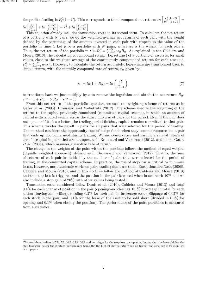
Figures 1(a) and 1(b) show an example of the historical prices between two cointegrated stocks,NATU3 and SSBR3, during the formation period and the subsequent trading period. The z-score isa measure of distance from the long run equilibrium in terms of standard deviations and it crossesthe 2 standard deviation threshold more than 6 times during the trading period, indicating thatthe spread widens and shortens very frequently in a given 6 month period.

9


�

��

��

��

��

�

��

��

��

��

(a) Historical Price of NATU3 and SSBR3 between july

2011 and december 2012.

��

��

��

��

�

�

�

�

��

��

(b) Z-score between NATU3 and SSBR3 between july

2011 and december 2012.

Figure 1. An example for the brazilian stock market.

The portfolios created had between 5 to 20 pairs selected be it through the cointegration orthe distance method. Table 3 first half shows the summary statistics for the portfolios createdthrough both methodologies. As is expected, the average number of pairs opened increases withthe number of pairs in the portfolio. Nonetheless, all other statistics remain very similar, except forthe average price deviation for opening pairs, which also increases with the number of pairs in theportfolio. Given that every extra cointegrated pair or maatched pairs through SSD included in theportfolio has a smaller sharpe ratio and more likely to diverge by more due to its stocks ’weaker’comovement, it is probable that those pairs tend to diverge more from their long run equilibrium,explaining the higher average price deviation. Each cointegrated pair had on average between 2.97and 2.3 round trip trades depending on the size of the portfolio, which means that each pair wastraded on average more than 2 complete times each 6 months period.

Since the prices used for the distance method are normalized, the average standard deviationsare not directly comparable between the pairs selection method in Table 3. However, the averagenumber of pairs opened is comparable, and it shows that the distance method is more ’triggerhappy’ than the cointegration method. This selection method starts, for the 20 pairs portfolio, a1200 pairs more than the cointegration method, possibly resulting in over trading and incurringin excessive transaction costs. Also, these pairs remain open on average around 25 trading days,while in the cointegration method the pairs remain open on average 16,8 days, indicating thatthe distance method not only opens more pairs in a given period, it also stays longer in a openposition. Each pair was traded on average between 3.5 and 4 times each 6 months for the distancemethod, meaning that in a period of an average of 120 trading days, there was room for an averageof opening a pair up to 4 times and closing it also 4 times.

The excess returns are for the whole trading out of sample, between july 1996 and december2012 already discounted for transaction costs and slippage effects. Some periods exhibit less than20 cointegrated pairs, specialy the years between 1996 and 2002, consequently when applicable, weused the maximun number available of pairs to form a portfolio.The average annualized return forthe cointegrated pairs dimishes with the inclusion of more pairs, from 23% with 5 pairs to 18,37%when a portfolio consists of 20 pairs. Nonetheless, the average annualized volatility also dimishes,from 11,20% with a portfolio of 5 pairs to 7,9% when with 20 pairs in a portfolio. Consequently, theSharpe Ratio for the whole sample is higher for the top 20 pairs (2,11) due to the lower volatility,which more than compensate the lower average annualized return (18,37%). The cumulative returnbetween 1996 and 2012, range from 1364% for a portfolio of 20 pairs to 2499% for a portfolio with5 pairs. The correlation with the market is slightly negative and not significantly different fromzero, exactly what we want and would expect from a market neutral strategy. The share of dayswith negative returns is between 36% and 38% and very inferior to the 48% share of days withnegative returns in the Ibovespa. The maximum drawdown is also included in the summary reaching21,68% for the all cointegrated pairs portfolios. This is a simple measure thay indicates the largestcumulative loss after a given maximun of a cumulative positive rallying of the returns, signaling

10


how fast the leverage can increase, much smaller than the 65% drawdown of the Ibovespa.The summary statistics for the pairs selected through the distance method are presented on table

3. The volatility for the portfolios created through this method is over 10% for all 3 portfolios,higher than for the cointegration method portfolios, which range between 11,2% and 7,9%, but theannualized average return are all inferior to the cointegrated pairs portfolios, ranging between 3,2%and 6,4%, a little less than a third when compared with the cointegration method. The consequenceis that the Sharpe Ratios are very small, not statistically different from the Ibovespa Sharpe ratioof 0,58 for the whole sample. Even though the strategy is market neutral with a close to zeroSpearman rho for all 3 portfolios, the maximum drawdown is mostly higher than the ones thatoccur in the cointegration method. Not only, the share of days with negative returns is over 48%for all porfolios, similar to the Ibovespa performance, with all these statistics indicating that thisstrategy is not superior than buying and holding the market index.

Table 3. Excess returns of unrestricted pairs trading strategies: brazilian dataset

Note: This table reports a summary statistics of the excess returns on portfolios of pairs betweenJanuary 1995 and December 2012 (216 observations). Pairs are formed over a 12-month period accord-ing to a minimum-distance criterion and then traded over the subsequent 6-month period. Pairs areopened when prices diverge by two standard deviations. CAPM-estimates are from the OLS regressionanalysis.

Mehodology Distance approach Cointegration approach

Pairs Portfolio Top 5 Top 10 Top 20 Top 5 Top 10 Top 20

Total number of pairs opened 592 1289 2757 506 897 1577Total number of 6 month trading periods 34 34 34 34 34 34Average price deviation for opening pairs 0.114 0.140 0.172 0.590 0.654 0.695Average no of pairs opened each 6 mo period 17.41 37.91 81.08 14.88 26.38 46.38Average number of pairs traded in months when at least one pair opened 3.588 3.906 4.177 3.265 3.159 3.092Average number of round-trip trades per pair 3.482 3.791 4.054 2.977 2.638 2.319Standard deviation of round-trips per pair 2.099 2.108 3.208 1.843 1.942 1.937Average time pairs are open in days 27.60 25.36 23.78 16.54 16.82 16.94Median time pairs are open in days 13.50 14.00 14.00 12.00 12.00 13.00Average time pairs are open in months 1.314 1.208 1.132 0.788 0.801 0.807Standard deviation of time open per pair in days 33.18 29.57 26.22 13.63 14.36 14.08Standard deviation of time open per pair in months 1.580 1.408 1.249 0.649 0.684 0.671Share of negative excess returns 0.485 0.484 0.498 0.368 0.377 0.378

Average Annualized Return (in %) 4.924 6.460 3.200 23.00 19.77 18.37Average Annualized Volatility (in %) 13.01 11.52 10.70 11.20 9.24 7.90Total Sample Sharpe Ratio 0.370 0.544 0.294 1.850 1.950 2.110Largest Daily Return (in %) 4.240 4.230 4.020 9.600 9.600 9.600Lowest Daily Return (in %) -6.380 -4.200 -3.750 -4.430 -3.920 -3.840Cumulative Profit (in %) 90.00 148.00 51.88 2,499.00 1,642.00 1,364.00Spearman Correlation Rho with Ibovespa 0.051 0.062 0.095 -0.009 -0.013 -0.014CAPM beta (β-market ) 0.029 0.027 0.040 -0.004 -0.003 -0.004Annual Skewness 0.821 1.291 1.248 1.010 1.130 1.740Annual Kurtosis 3.056 4.427 4.407 3.730 5.060 8.910Maximun Drawdown (in %) 31.78 18.65 22.44 21.68 21.68 21.68

Table 4 shows the results found for the American data set for the whole sample period betweenjanuary 1962 and december 2012. The average number of pairs opened, just like in the otherdatabases, also increases with the number of pairs in the portfolio. However, both strategies performin a very similar way in terms of the number of pairs that open and close each trading period. Thedistance method does not starts a significant number of pairs more than the cointegration method,with the portfolios of 5, 10 and 20 pairs starting, respectivelly 17, 32, and 74 pairs on average forthe distance method. Slightly more than the 16, 31 and 64 pairs on average for the cointegrationmethod with the same portfolio size. The average number of round trips per pair was between 3and 4 for both strategies, with all portfolios having a similar number o round trips. The averagetime pairs remain open in the both method is very similar, betwenn 7 and 10, with the standarddeviation slight higher for the distance method portfolios. The descriptive results for the United

11


States show a tendency towards similarity betwenn both strategies in terms of round trips, mediantime pairs are open and they even have similarshare of negative excess returns.

The average annualized excess return for both strategies dimishes with the inclusion of morepairs, from 10.47% with 5 pairs to 9.55% when a portfolio consists of 20 pairs in the distancemethod. Nonetheless, the average annualized volatility also dimishes, from 5.54% with a portfolioof 5 pairs to 3.13% when with 20 pairs in a portfolio. Consequently, the Sharpe Ratio for the wholesample is higher for the top 20 pairs (2.9) due to the lower volatility, which more than compensatethe lower average annualized return (9,55%). The cumulative return between 1962 and 2012, rangefrom 9184% for a portfolio of 20 pairs to 13331% for a portfolio with 5 pairs. The correlation withthe market is slightly positive and not significantly different from zero, exactly what we want andwould expect from a market neutral strategy. The share of days with negative returns is between35% and 44The maximum drawdown is also included in the summary reaching 21.14% for the 5pairs portfolios chosen by the distance method. This is a simple measure thay indicates the largestcumulative loss after a given maximun of a cumulative positive rallying of the returns, signalinghow fast the leverage can increase.

The summary statistics for the pairs selected through the cointegration method are presentedon table 4 also. The volatility for the portfolios created through this method is betwenn 5,4% and10,36% for all 3 portfolios, higher than for the distance method portfolios, and the annualizedaverage return are all inferior to the distance method pairs portfolios, ranging between3.7% and5.5%. The consequence is that the Sharpe Ratios are also low. The cointegration method strategyis market neutral with a market beta and a Spearman rho close to zero for all 3 portfolios and themaximum drawdown is mostly higher than the ones that occur in the cointegration method. Theshare of days with negative returns ranges between 26% and 34% for all cointegratied porfolios andare mostly similar to the distance method portfolios. In summary, the distance method performsbetter than the cointegration method for the United States, with most performance metrics beingsuperior and indicating a clear advantage.

Table 5 shows the results found for the european data set for the whole sample period betweenjanuary 1973 and december 2012. The average number of pairs opened, just like in the braziliandatabase, also increases with the number of pairs in the portfolio. However, the difference betweenboth strategies is smaller. The distance method does not starts a significant number of pairs morethan the cointegration method, with the portfolios of 5, 10 and 20 pairs starting, respectivelly 27,54, and 105 pairs on average for the distance method. Slightly more than the 24, 49 and 95 pairson average for the cointegration method with the same portfolio size. The average number of roundtrips per pair was slightly over 5 for the distance method and slightly under 5 for the cointegrationmethod, still indicating that the former tends to open more pairs then the latter. The average timepairs remain open in the distance method portfolio is around 10 days, almost double than the 5.3to 5.9 average days the cointegration pairs remain open, and the standard deviation of the timeopen in days is around 20 days, while for the cointegration method is a little over 6 days, with suchresult pointing towards the tendency for the distance approach to be more ”trigger happy” and atthe same remain longer on a given pair.

The average annualized excess return for the cointegrated pairs dimishes with the inclusion ofmore pairs, from 13.73% with 5 pairs to 11.19% when a portfolio consists of 20 pairs. Nonetheless,the average annualized volatility also dimishes, from 8.41% with a portfolio of 5 pairs to 6.15%when with 20 pairs in a portfolio. Consequently, the Sharpe Ratio for the whole sample is higherfor the top 20 pairs (2.3) due to the lower volatility, which more than compensate the lower averageannualized return (11.19%). The cumulative return between 1973 and 2012, range from 6479% fora portfolio of 20 pairs to 14,600% for a portfolio with 5 pairs. The correlation with the market isslightly positive and not significantly different from zero, exactly what we want and would expectfrom a market neutral strategy. The share of days with negative returns is between 26% and 38%and similar to the 29,9% share of days with negative returns in the MSCI Europe excluding UK andSwitzerland Index. The maximum drawdown is also included in the summary reaching 37,95% forthe 5 pairs cointegrated portfolios. This is a simple measure thay indicates the largest cumulative

12


Table 4. Excess returns of unrestricted pairs trading strategies: USA dataset

Nota: This table reports a summary statistics of the monthly excess returns on portfolios of pairsbetween January 1962 and December 2012 (600 observations). Pairs are formed over a 12-month periodaccording to a minimum-distance criterion and then traded over the subsequent 6-month period. airs areopened when prices diverge by two standard deviations. CAPM-estimates are from the OLS regressionanalysis.

Methodology Distance approach Cointegration approach


Total number of pairs opened 1784 3233 7425 1624 3190 6479Total number of 6 month trading periods 100 100 100 100 100 100Average price deviation for opening pairs 0.0215 0.0279 0.0304 0.414 0.4180 0.4172Average no of pairs opened each 6 mo period 17.84 32.33 74.25 16.24 31.9 64.79Average number of pairs traded in months when at least one pair opened 3.5752 3.2362 3.7144 3.248 3.19 3.2444Average number of round-trip trades per pair 3.5680 3.233 3.7125 3.2480 3.19 3.2395Standard deviation of round-trips per pair 2.6607 2.4728 2.2231 1.9125 1.8765 1.8966Average time pairs are open in days 11.3879 12.7145 21.3436 9.322 9.5558 9.5367Median time pairs are open in days 7 8 10 8 8 8Average time pairs are open in months 0.5423 0.6055 1.0164 0.4439 0.455 0.4541Standard deviation of time open per pair in days 10.6119 10.9617 28.1507 6.1963 6.4086 6.48Standard deviation of time open per pair in months 0.5053 0.5220 1.3405 0.2951 0.3052 0.3086Share of negative excess returns 0.3552 0.4138 0.4398 0.3264 0.4027 0.4348

Average Annualized Return (in %) 10.4778 9.772 9.55 5.5728 3.7912 4.2045Average Annualized Volatility (in %) 5.5407 4.1152 3.1358 10.3695 7.4568 5.4070Total Sample Sharpe Ratio 1.798 2.2662 2.9097 0.5231 0.4991 0.7618Largest Daily Return (in %) 4.170 1.90 2.71 6.78 3.71 2.58Lowest Daily Return (in %) -3.03 -3.22 -1.61 -6.46 -4.47 -2.97Cumulative Profit (in %) 13,331.00 9,923.00 9,188.00 1,047.00 458.00 627.00Spearman Correlation Rho with MSCI 0.0163 0.0211 0.013 0.0123 0.0163 0.0143CAPM beta (β-market ) 0.0184 0.01 0.0104 0.0271 0.0222 0.0174Annual Skewness 1.0844 0.3914 0.3033 1.0311 0.7708 1.6479Annual Kurtosis 4.2085 2.2037 2.2352 4.3151 2.9412 8.9737Maximun Drawdown (in %) 21.14 19.48 14.99 26.55 34.76 28.85

loss after a given maximun of a cumulative positive rallying of the returns, signaling how fast theleverage can increase, much smaller than the 65,85% drawdown of the MSCI Index.

The summary statistics for the pairs selected through the distance method are presented on table5 also. The volatility for the portfolios created through this method is betwenn 3,4% and 5,2% forall 3 portfolios, lower than for the cointegration method portfolios, which range between 4,5%and 8,4%, but the annualized average return are all inferior to the cointegrated pairs portfolios,ranging between 6,3% and 7,8%. The consequence is that the Sharpe Ratios are are increasingwith the portfolio’s size. The distance method strategy is market neutral with a market beta anda Spearman rho close to zero for all 3 portfolios and the maximum drawdown is mostly lower thanthe ones that occur in the cointegration method. The share of days with negative returns rangesbetween 36% and 41% for all porfolios higher than the MSCI Index and the cointegration method.

5. Pairs trading performance evaluation

5.1. Bootstrap for assessing pairs trading performance

In order to evaluate the performance of the strategies, we compare it to a naive strategy, i.e.,we create bootstrapped return series in which the signal to start the strategy of pairs trading isinserted,and the performance of such a strategy is monitored and compared to the performanceof the original series of returns. We follow the method used by Gatev et al. (2006), Caldeira andMoura (2013), in which the bootstrap initiates at the time at which the signal is sent to begintrading pairs. In each bootstrap, the original series is replaced by two series of random assetssimilar to the assets earlier, similarity being defined as returns in the previous month belonging to

13


Table 5. Excess returns of unrestricted pairs trading strategies: european dataset

Nota: This table reports a summary statistics of the monthly excess returns on portfolios of pairsbetween January 1973 and December 2012 (468 observations). Pairs are formed over a 12-month periodaccording to a minimum-distance criterion and then traded over the subsequent 6-month period. airs areopened when prices diverge by two standard deviations. CAPM-estimates are from the OLS regressionanalysis.

Methodology Distance approach Cointegration approach


Total number of pairs opened 2108 4264 8246 1930 3851 7427Total number of 6 month trading periods 77 77 77 77 77 77Average price deviation for opening pairs 0.017 0.019 0.021 0.299 0.341 0.390Average no of pairs opened each 6 mo period 27.02 54.66 105.71 24.74 49.37 95.21Average number of pairs traded in months when at least one pair opened 5.475 5.538 5.355 5.039 5.021 4.896Average number of round-trip trades per pair 5.405 5.467 5.286 4.949 4.937 4.761Standard deviation of round-trips per pair 3.400 3.527 3.587 2.838 2.777 2.832Average time pairs are open in days 10.08 9.776 10.24 5.351 5.593 5.907Median time pairs are open in days 3.00 3.00 3.00 3.00 3.00 3.00Average time pairs are open in months 0.48 0.466 0.488 0.255 0.266 0.281Standard deviation of time open per pair in days 20.30 19.22 19.54 5.96 6.22 6.48Standard deviation of time open per pair in months 0.967 0.915 0.931 0.284 0.297 0.309Share of negative excess returns 0.364 0.405 0.410 0.262 0.334 0.385

Average Annualized Return (in %) 6.391 7.591 7.814 13.73 12.65 11.19Average Annualized Volatility (in %) 5.261 4.229 3.414 8.410 6.156 4.59Total Sample Sharpe Ratio 1.178 1.731 2.204 1.530 1.936 2.300Largest Daily Return (in %) 4.170 2.340 1.960 6.810 3.880 2.220Lowest Daily Return (in %) -5.420 -2.710 -1.890 -7.390 -3.690 -3.150Cumulative Profit (in %) 1,018.00 1,683.00 1,860.00 14,602.00 10,629.00 6,479.00Spearman Correlation Rho with MSCI 0.019 0.013 0.013 0.009 0.006 0.029CAPM beta (β-market ) 0.004 0.003 0.002 0.001 0.003 0.004Annual Skewness 1.586 1.437 1.399 1.220 0.659 0.540Annual Kurtosis 7.769 6.118 5.256 5.150 2.750 2.320Maximun Drawdown (in %) 21.54 13.47 30.48 37.95 27.20 28.85

the same decile. Thus, the difference in performance of the original assets and simulated give anindication of performance. The net return of the naive strategy is given by:

Rnaivet =N∑i=1

witrit + 2N ln

(1− C1 + C

)(8)

The results were calculated in every 6 month trading period and are withheld due to spaceconstraints and can be obtained by contacting the author. We bootstrap each period 2500 for eachof the pairs selection methodology and for each portfolio size, and found that both strategies obtainstatisticallly significant positive performance when compared to a naive trader for both countries.In other words, the pairs trading strategies based on the selection of pairs through cointegration andthrough the distance method have a superior performance when compared to the random selectionof pairs of stocks to be traded. The average returns on the random pairs is slightly negative, possiblydue to the inclusion of transaction costs, and the standard deviations are large compared to thepairs trading portfolio’s standard deviations.

5.2. Hypothesis testing for the difference between the Sharpe Ratios

Given that the objective of this paper is to compare the performance of two pairs selection methods,we must use a metric in order to assess if any of the strategies has a superior performance. In orderto test the statistical significance of the difference between the Sharpe ratios of both strategies weuse the methodology proposed in Ledoit and Wolf (2008) and obtain the p-values of the stationarybootstrap of Politis and Romano (1994) with B = 1000 bootstrap resamples and block length b=

14


5.The whole sample result for the difference between Sharpe ratios through the methodology pro-

posed by Ledoit and Wolf (2008) indicates that for Brazil, the cointegration method is superiorduring the whole sample period to the distance method. However, for the subperiods the resultsare not as robust, with most subperiods results, available upon request, indicating that the coin-tegration method does not deliver a statistically significant higher Sharpe Ratio which hints atthe fact that some subperiods might be driving the full sample results, or that the performance isslightly superior in each period, but not statistically higher due to sample limitations, since the sizeof most subperiods sample is 120 compared to the whole period that comprises 4087 observations.For europe the results also indicate that for the whole sample period the cointegration strategyis superior when using a portfolio consisting of 10 and 20 pairs. However for the 5 pairs portfoliothe p-value of the statistic calculated is 0.107, and the cointegration strategy cannot be consideredsuperior. Also, for the 6 month subperiods the cointegration strategy in most subsample periodsis not superior, with the results most likely being driving by some subperiods. These findings hintthat the cointegration strategy may be superior to the distance method in some periods, while thedistance method may be superior in other subperiods, but on average the cointegration methoddelivers a higher Sharpe Ratio. For the USA the results are the other way around. The distancemethod Sharpe Ratio is statistically superior than on the cointegration method, for all 3 portfoliosizes. However, again as in Brazil and for Europe, the results in the subperiods are mixed, withthe distance method not being superior in all 6 month subperiods (tables available upon request).

Table 6. P-value of the test statistic pair wise between the portfolios for the SharpeRatio for Brazil, total sample

P-Value Top 5 pairs Top 10 pairs Top 20 pairs

All Sample Robust Sharpe Ratio Difference Test

0.000 0.000 0.000

Table 7. P-value of the test statistic pair wise between the portfolios for the SharpeRatio for USA, total sample



0.000 0.000 0.000

Table 8. P-value of the test statistic pair wise between the portfolios for the SharpeRatio for Europe, total sample



0.107 0.010 0.001

15


6. Conclusion

In this paper we compared two methodologies for the strategy called pairs trading. The distancemethod presented in Gatev et al. (2006) and the cointegration method used by Caldeira and Moura(2013), for the american stock market between 1962 and 2012, for the brazilian stock marketbetween 1996 and 2012 and for the european market between 1973 and 2012. We create portfolioscomprising 5, 10 and 20 pairs for each method, and bootstrap the results in order to compare thetheir performance. The pairs were ranked by their in sample sharpe in the cointegration methodand by the smallest to the highest SSD for the distance method in order to form the portfolios. Thesignal to open the position out of sample was given whenever the distance between the stocks on agiven pair crossed the 2 standard deviation threshold. Both methodologies had a good performancewhen compared to a naive trader that randomly selection pairs to trade on a given period. ForBrazil, the cointegration method had a cumulative return between 1996 and 2012 of up to 2499%,while the distance method had up to 148% of cumulative return. When compared to each other,the cointegration method had a clear, statistically significant higher average annualized return,with a superior Sharpe Ratio, and, most of the time, a statistically significant inferior volatility.Both strategies can be considered market neutral, with a close to zero spearman correlation withthe market.

For Europe, while the results were not so clear cut, they also pointed towards the cointegationmethod being superior, delivering up to 14.602% of cumulative returns against 1.860% for the dis-tance method. The Sharpe Ratio was also considered superior for the whole sample period, althoughin some subsamples both strategies were very similiar. Both strategies had an excess returns supe-rior than a naive trader. For the United States, the results were very different, indicating that thedistance method is superior, delivering up to 13.331% of cumulative return, more than the 1.047%of the cointegration method. Considering that this strategy is self-financed, since the cash obtainedby shortening a stock is used to buy the long stock in the pair, these results are encouraging andindicate a clear path for more research regarding the drivers of such difference in performance, theoptimality of the trading thresholds and the stability of the cointegration parameters.

16


References

Alexander, C., Optimal hedging using cointegration. Philosophical Transactions of the Royal Society ofLondon. Series A: Mathematical, Physical and Engineering Sciences, 1999, 357, 2039–2058.

Alexander, C. and Dimitriu, A., The cointegration alpha: Enhanced index tracking and long-short equitymarket neutral strategies. SSRN eLibrary, 2002.

Alexander, C. and Dimitriu, A., Indexing and statistical arbitrage. Journal of Portfolio Management, 2005,31, 50–63.

Andrade, C.S., di Pietro, V. and Seasholes, M.S., Understanding the Profitability of Pairs Trading. Technicalreport, UC Berkeley Haas School,, 2005.

Avellaneda, M. and Lee, J.H., Statistical arbitrage in the US equities market. Quantitative Finance, 2010,10, 761–782.

Bessler, D.A. and Yang, J., The structure of interdependence in international stock markets. Journal ofInternational Money and Finance, 2003, 22, 261–287.

Bowen, D., Hutchinson, M. and O’Sullivan, N., High frequency equity pairs trading: transaction costs, speedof execution and patterns in returns. Journal of Trading, 2010, 5, 31–38.

Broussard, J.P. and Vaihekoski, M., Profitability of pairs trading strategy in an illiquid market with multipleshare classes. Journal of International Financial Markets, Institutions and Money, 2012, 22, 1188–1201.

Caldeira, J.F. and Moura, G.V., Selection of a Portfolio of Pairs Based on Cointegration: A StatisticalArbitage Strategy. Brazilin Review of Finance, 2013, 11, 49–80.

Do, B. and Faff, R., Are pairs trading profits robust to trading costs?. Journal of Financial Research, 2012,35, 261–287.

Do, B., Faff, R. and Hamza, K., A new approach to modeling and estimation for pairs trading. In Proceedingsof the Proceedings of 2006 Financial Management Association European Conference, 2006.

Do, B. and Faff, R.W., Does simple pairs trading still work?. Financial Analysts Journal, 2010, 66, 83–95.Elliott, R.J., Van Der Hoek, J. and Malcolm, W.P., Pairs trading. Quantitative Finance, 2005, 5, 271–276.Engelberg, J., Gao, P. and Jagannathan, R., An anatomy of pairs trading: the role of idiosyncratic news,

common information and liquidity. In Proceedings of the Third Singapore International Conference onFinance, 2009.

Engle, R.F. and Granger, C.W., Long-run economic relationships: Readings in cointegration, 1991, OxfordUniversity Press.

Galenko, A., Popova, E. and Popova, I., Trading in the Presence of Cointegration. The Journal of AlternativeInvestments, 2012, 15, 85–97.

Gatarek, L., Hoogerheide, L. and van Dijk, H.K., Return and Risk of Pairs Trading using a Simulation-basedBayesian Procedure for Predicting Stable Ratios of Stock Prices. Tinbergen Institute Discussion Papers14-039/III, Tinbergen Institute, 2014.

Gatev, E., Goetzmann, W.N. and Rouwenhorst, K.G., Pairs trading: Performance of a relative-value arbi-trage rule. Review of Financial Studies, 2006, 19, 797–827.

Guidolin, M., Hyde, S., McMillan, D.G. and Ono, S., Non-linear predictability in stock and bond returns:When and where is it exploitable?. International Journal of Forecasting, 2009, 25, 373–399.

Hendershott, T., Jones, C.M. and Menkveld, A.J., Does Algorithmic Trading Improve Liquidity?. Journalof Finance, 2011, 66, 1 – 33.

Huck, N., Pairs trading and outranking: The multi-step-ahead forecasting case. European Journal of Oper-ational Research, 2010, 207, 1702–1716.

Jacobs, B.I., Levy, K.N. and Starer, D., Long-Short Portfolio Management: An Integrated Approach. TheJournal of Portfolio Management, 1999, 25, 23–32.

Johansen, S., Statistical analysis of cointegration vectors. Journal of economic dynamics and control, 1988,12, 231–254.

Ledoit, O. and Wolf, M., Robust performance hypothesis testing with the Sharpe ratio. Journal of EmpiricalFinance, 2008, 15, 850–859.

Lo, A.W. and MacKinlay, A.C., Stock Market Prices do not Follow Random Walks: Evidence from a SimpleSpecification Test. Review of Financial Studies, 1988, 1, 41–66.

Lo, A.W. and MacKinlay, A.C., Maximizing Predictability In The Stock And Bond Markets. MacroeconomicDynamics, 1997, 1, 102–134.

Lucas, A., Strategic and Tactical Asset Allocation and the effect of long-run equilibrium relations. SerieResearch Memoranda 0042, VU University Amsterdam, Faculty of Economics, Business Administration

17


and Econometrics, 1997.Nuti, G., Mirghaemi, M., Treleaven, P. and Yingsaeree, C., Algorithmic Trading. Computer, 2011, 44, 61–69.Perlin, M.S., Evaluation of pairs-trading strategy at the Brazilian financial market. Journal of Derivatives

& Hedge Funds, 2009, 15, 122–136.Politis, D.N. and Romano, J.P., The stationary bootstrap. Journal of the American Statistical Association,

1994, 89, 1303–1313.Vidyamurthy, G., Pairs Trading: quantitative methods and analysis, Vol. 217, , 2004, Wiley.Yang, J., Kolari, J.W. and Sutanto, P.W., On the stability of long-run relationships between emerging and

US stock markets. Journal of Multinational Financial Management, 2004, 14, 233–248.Yuksel, A., Yuksel, S. and Muslumov, A., Pairs trading with turkish stocks. Middle East. Financ. Econ,

2010, 7, 38–54.

18

Documents

Is Pairs Trading Performance Sensitive to the Methodologies… · Caldeira and Moura (2013) in Brazil. Although many papers have been written about pairs trading, the literature lacks