NBER WORKING PAPER SERIES

IS SELL-SIDE RESEARCH MORE VALUABLE IN BAD TIMES?

Roger K. LohRené M. Stulz

Working Paper 19778http://www.nber.org/papers/w19778

NATIONAL BUREAU OF ECONOMIC RESEARCH1050 Massachusetts Avenue

Cambridge, MA 02138January 2014

We thank Marcin Kacperczyk, Oguzhan Karakas, Jeff Kubik, Massimo Massa, Roni Michaely, JayRitter, Stijin Van Nieuwerburgh, Paola Sapienza, Siew Hong Teoh, Mitch Warachka, Kent Womack,Frank Yu, Jialin Yu, an anonymous associate editor and two anonymous referees, participants at theAFA 2014 Philadelphia meetings and the 2013 SMU-SUFE Summer Institute of Finance Conference,and at a seminar at the University of Zurich for helpful comments. Brian Baugh, Andrei Gonçalves,and David Hauw provided excellent research assistance. Roger thanks the Sing Lun Fellowship andthe Sim Kee Boon Institute for Financial Economics at Singapore Management University for financialsupport. The views expressed herein are those of the authors and do not necessarily reflect the viewsof the National Bureau of Economic Research.

NBER working papers are circulated for discussion and comment purposes. They have not been peer-reviewed or been subject to the review by the NBER Board of Directors that accompanies officialNBER publications.

© 2014 by Roger K. Loh and René M. Stulz. All rights reserved. Short sections of text, not to exceedtwo paragraphs, may be quoted without explicit permission provided that full credit, including © notice,is given to the source.

Is Sell-Side Research More Valuable in Bad Times?Roger K. Loh and René M. StulzNBER Working Paper No. 19778January 2014, Revised November 2016JEL No. F14,F20,F24

ABSTRACT

Because uncertainty is high in bad times, investors find it harder to assess firm prospects and, hence,should value analyst output more. However, higher uncertainty makes analysts’ tasks harder so it isunclear if analyst output is more valuable in bad times. We find that, in bad times, analyst revisionshave a larger stock-price impact, earnings forecast errors per unit of uncertainty fall, reports are morefrequent and longer, and the impact of analyst output increases more for harder-to-value firms. Theseresults are consistent with analysts working harder and investors relying more on analysts in bad times.

Roger K. LohSingapore Management UniversityLee Kong Chian School of Business50 Stamford Rd, #04-01Singapore 178899Singaporerogerloh@smu.edu.sg

René M. StulzThe Ohio State UniversityFisher College of Business806A Fisher HallColumbus, OH 43210-1144and NBERstulz@cob.osu.edu

1

1. Introduction

Even though there is a large literature on sell-side analysts’ role as information intermediaries, this literature

mostly ignores the issue of whether the state of the economy affects the value of analyst output for investors.1

There are good reasons to believe that the usefulness and performance of sell-side analysts depend on the state

of the economy. It is well-known that in bad times such as recessions and crises, there is greater variation in

outcomes across firms and across time (see, for instance, Bloom (2009)). To the extent that the role of analysts

is to make sense of firms amidst the increased macro uncertainty, their role should be more important in bad

times and, consequently, they should work harder in bad times. At the same time, however, the increased

uncertainty may make it harder for analysts to perform their job. Further, the drop in trading volume and hence

broker profits in bad times may reduce performance rewards, leading to less motivated analysts. Hence, it is not

clear whether analyst output is more valuable in bad times than in good times. In this paper, we find that

analysts are indeed more valuable in bad times. The stock-price impact of their recommendation and earnings

forecast revisions is greater in bad times. We investigate possible explanations for this finding and conclude that

the evidence is consistent with analysts working harder and investors relying more on analysts in bad times.

We conduct our investigation using a sample of I/B/E/S Detail earnings forecasts from 1983-2014 and

recommendations from 1993-2014. We define bad times in multiple ways. The most obvious approach is to use

prominent crises that have occurred in the last two decades, such as the October 1987 crash, the LTCM crisis of

1998, and the credit crisis of 2007-2009. We also define bad times as recession periods marked by the National

Bureau of Economic Research (NBER), and as periods of high uncertainty according to the Baker, Bloom, and

Davis (2016) policy uncertainty index (from www.policyuncertainty.com). Our measure of the value of analyst

1 For example, Womack (1996), Barber, Lehavy, McNichols, and Trueman (2001), Kecskés, Michaely, and Womack

(2016) show that stock prices react to the release of analyst recommendations and a drift follows afterwards. Loh and Stulz

(2011) show that some recommendation changes exert a large noticeable change in the firm’s stock price and these

recommendations can impact the firm’s information environment. Bradley, Clarke, Lee, and Ornthanalai (2014) report that

recommendations are more likely than earnings announcements or company earnings guidance to cause jumps in intraday

stock prices. Others find that analyst coverage reduces information asymmetry, improves visibility (Kelly and Ljungqvist

(2012)), disciplines credit rating agencies (Fong, Hong, Kacperczyk, and Kubik (2014)), and affects corporate policies

(Derrien and Kecskés (2013)).

2

output is the price impact, which shows the extent to which analyst signals affect investors’ assessment of the

value of firms and hence is a measure of how analysts contribute to the information environment of firms.

Using the average two-day abnormal returns to stock recommendation changes, we find that analysts are

more impactful during bad times for both downgrades and upgrades. Further, using the definition of influential

recommendations in Loh and Stulz (2011), which effectively treats recommendation changes as influential if the

stock-price reaction is statistically significant, we find robust evidence that both upgrades and downgrades are

more likely to be influential during bad times compared to good times. We also find that the market reacts more

strongly to earnings forecast revisions during bad times. Our evidence of greater analyst impact during bad

times is robust to controls for firm and analyst characteristics, including analyst fixed effects. We conclude that

analyst output is more useful for investors in bad times in that it moves stock prices more.

We perform several robustness tests for our results. Our focus is on macro instead of firm-specific bad times

because macro bad times are economically important and because they are more likely to be exogenous to

analysts. Prior studies like Frankel, Kothari, and Weber (2006) and Loh and Stulz (2011) show that analyst

reports are more informative when firm-level uncertainty is higher. While we already control for firm-level

uncertainty in our results, we want to be sure that it is macro (i.e. market-level) uncertainty that drives our

results. We decompose a firm’s total stock return volatility into market, industry, and firm-specific components.

We find that the increased impact of recommendation changes in times of high uncertainty is most robust when

the market component is used to define high uncertainty. Second, we investigate whether the market simply

reacts more to all types of firm news in bad times (e.g., Schmalz and Zhuk (2015) find that reactions to earnings

announcements are larger in recessions). Adapting the methodology in Frankel et al. (2006), we regress a

stock’s daily absolute returns on a comprehensive set of dummy variables that represent important firm news

events, namely, recommendation changes, reiterations, earnings announcements, earnings guidance, dividend

announcements, and insider trades. Interacting these news dummies with bad times indicators, we show that not

all firm news events are associated with greater bad times impact. Importantly, the market reacts more to

recommendation changes (and reiterations) in bad times even after all other news events and their interactions

3

with bad times are controlled for. Hence we believe our finding that analysts have greater impact in bad times is

both novel and robust.

We also find that the absolute forecast errors of analysts increase during bad times, which makes it puzzling

that their output would have more impact on prices. We show, however, that the traditional metrics of analyst

precision are not appropriate to compare precision across good and bad times. The relevant measure of precision

for investors is one that takes into account the underlying uncertainty. This is easily seen in a simple Bayesian

model. Consider investors who receive a new signal from analysts. The extent to which that signal will change

their priors depends on the weight that investors put on the new signal and on the weight they put on their prior

(e.g., see Pastor and Veronesi (2009)). As the precision of the signal increases relative to the uncertainty

associated with their prior, they put more weight on the signal. Hence, in bad times, investors will put more

weight on a signal from an analyst if the ratio of the precision of the signal to the uncertainty of the prior

increases. Such an outcome could occur if the precision of the signal is lower in bad times as long as the

precision of the signal falls less than the increase in the uncertainty about the prior. A useful way to put this is

that the relevant measure of forecast error is a measure of forecast error per unit of uncertainty.

Using prior volatility to normalize absolute forecast errors, we find that this adjusted forecast precision

actually increases during bad times (scaling by prior volatility is similar to the approach we used to define

influential recommendation changes). Importantly however, showing that analyst forecast precision increases

when measured against the underlying uncertainty does not mean that analysts automatically become more

useful to investors. Specifically, it could be that investors rely less on analysts in bad times if they have better

alternative sources of information. For instance, Kacperczyk and Seru (2007) show that how much investors rely

on public information depends on the precision of their private information. Hence, in their model, if the analyst

signal is public information, investors would rely less on analysts in bad times if investors themselves have

better private information.

We examine five possible, non-mutually exclusive, reasons why analysts have more impact in bad times.

First, we develop and investigate an analyst reliance hypothesis that builds on Kacperczyk and Seru (2007). Our

analyst reliance hypothesis predicts that investors rely more on analysts for their information during bad times.

4

During bad times, investors have to understand how the macro situation with its attendant uncertainty affects the

prospects of firms. Because of the greater macro uncertainty, possible outcomes are more extreme and,

consequently, have potentially a greater impact on firms than during good times. Everything else equal, we

would expect greater demand for analyst output that helps investors sort out the impact of ongoing macro shocks

during bad times compared to good times. If investors already know much about a stock, analysts have less to

contribute. Consequently, when analyst output is more valuable, it will be especially more valuable for more

opaque stocks. It follows that the cross-sectional implication of the analyst reliance hypothesis is that the extent

to which analyst output becomes more valuable in bad times is inversely related to the quality of the information

environment for a stock and, therefore, the value of analyst output increases relatively more for stocks of more

opaque firms in bad times (namely, stocks with no company guidance, low institutional ownership, high

idiosyncratic risk, small size, no options traded, or low coverage). We find supportive evidence that the

increased impact of analysts in bad times is higher for stocks with a more opaque information environment.

The analyst reliance hypothesis does not assume that analysts change what they do in bad times. Rather,

analysts become more important for investors because investors face challenges that they do not face in good

times and analysts help them deal with these challenges. However, it is plausible that analysts also change what

they do during bad times. The next three hypotheses are about changes in analyst output in bad times. Our

second possible explanation for the increased impact of analysts in bad times is that analysts could be working

harder in bad times because of career concerns. Glode (2011) explains the better performance of mutual funds in

bad times by the fact that investment managers work harder to produce better payoffs because investors have

higher marginal utility in bad times. If the greater uncertainty in bad times causes investors to value analyst

signals more, analysts might also work harder to produce better signals in bad times.2 However, rewards for

better performance might be limited in bad times when bonus pools shrink and analysts’ employers face

financial difficulties due to reduced profits. As a result of these two opposing forces, there is no clear empirical

prediction as to whether analysts can be expected to work harder in bad times or not. We find that the stock

2 This channel is less direct for analysts compared to fund managers. Investors can directly reward good fund managers

with more inflows or less outflows. Investors instead can only indirectly reward good analysts through the analyst

reputation channel.

5

volatility-adjusted precision of analysts’ earnings forecasts goes up during bad times. This implies that analysts

work harder to produce better forecasts in bad times. To investigate for more tangible evidence of whether they

work harder, we find that analysts indeed revise their earnings forecasts more frequently and write longer

reports in bad times. Further, using regressions that examine analyst attrition, we find evidence that analysts are

more likely to leave the I/B/E/S database during bad times. This attrition risk could provide an incentive for

analysts to work harder during bad times. Since analysts produce better output in industries with more analyst

competition (Merkley, Michaely, and Pacelli (2016)), we would expect analysts to work harder in industries

with more analyst competition in bad times and hence that their impact would increase more in such industries.

We find strong supportive results for downgrades.

Third, we investigate whether analysts use different skills in bad times. Kacperczyk, Van Nieuwerburgh,

and Veldkamp (2014) find that mutual fund managers display more market-timing skills than stock-picking

skills during bad times. It is not clear if analysts also produce more information in bad times that is common

across firms when such common (sector/macro) information is more valued by investors. To investigate this, we

examine if a recommendation revision on a single firm impacts peer firms. This spillover might occur if part of

the information in the revision reflects the analyst’s forecast of the common factor. We find some evidence that

in bad times the spillover effect of downgrades on peer firms is larger than it is during good times. There is no

difference in the spillover effect of upgrades in bad times compared to good times. Hence part of the increased

influence of analysts in bad times, particularly for their downgrades, might come from an increased effort to

collect and produce negative macro/sector information.

Fourth, there has been much work on potential analyst conflicts of interests (for a review of some of the

evidence, see Mehran and Stulz (2007)). If analyst potential conflicts from investment banking are less

important in bad times because of lower deal flow, analyst output might become less distorted and hence more

valuable. To investigate this, we examine if forecast bias (i.e. the signed forecast error) is different in bad times.

If conflicts have less bite in bad times, analysts might be less optimistic in bad times than in good times. We

find little support for this hypothesis as the forecast bias is either no different in bad times, or even more

optimistic. We also explore whether the increased impact of analysts in bad times is related to the type of broker

6

the analyst works for. In particular, we find that the increased influence of analysts in bad times generally holds

for independent brokers as well as for brokers with investment banking business. Overall, we do not find

consistent evidence that the conflicts of interest hypothesis is helpful in explaining our results.

Our final and fifth potential explanation for the greater impact of analysts is that it has nothing to do with

analyst output per se but is the product of overreaction by investors. Overreaction could be more likely in bad

times due to lower liquidity so that trading on analyst revisions causes a temporary price pressure effect when

liquidity providers are less able to accommodate the order flow. Alternatively, arbitrageurs might be more

constrained in bad times, so that they cannot counteract overreaction by some investors as effectively as they

can in good times. We investigate whether stock-price drift after revisions differs in bad times compared to good

times and we find very little difference. Importantly, the stock-price drift after revisions does not exhibit

reversals in good or bad times. Hence, overreaction is an unlikely explanation for our results.

Our paper is not the first to make the point that economic agents find signals more valuable in bad times.

Kacperczyk, Van Nieuwerburgh, and Veldkamp (2015) derive such a result for skilled fund managers, i.e.,

managers who have access to valuable signals. They show that “[b]ecause asset payoffs are more uncertain,

recessions are times when information is more valuable.” In their model, fund managers allocate more attention

to aggregate shocks in bad times because of the increase in aggregate uncertainty. Since the risk premium is

higher in bad times, skilled managers’ greater attention to aggregate shocks in bad times leads them to perform

better in bad times. In good times, when aggregate uncertainty is lower and the risk premium is lower, fund

managers focus more on stock picking and pay more attention to signals about individual stocks. Kacperczyk et

al. (2014) find empirical support for their prediction that skilled managers are better at market timing in bad

times and better at stock selection in good times.

A few papers have examined aspects of the impact of crises on analyst output. However, none of them tests

the hypotheses that we focus on and are as comprehensive in showing that analyst revisions of recommendations

and earnings forecasts are more influential in bad times, or showing that it is the macro nature of bad times that

matters. Arand and Kerl (2012) examine analysts’ earnings forecasts and recommendations around the credit

crisis and find that, although forecast accuracy dropped, investors continued to react to revisions in

7

recommendations. Amiram, Landsman, Owens, and Stubben (2014) examine analyst forecast timeliness during

periods of high market volatility and find that analysts are less timely and underreact to news in those periods.

However, they also find that forecast revisions in these periods actually have more impact in reducing

information asymmetry measured by bid-ask spreads. Hope and Kang (2005) also find that forecast errors are

higher during bad times. While these papers conclude that investors wrongly pay attention to analysts who

appear to be more inaccurate in bad times, we show that, controlling for the underlying uncertainty, analysts are

actually more precise during bad times and investors rightly react more strongly to analyst revisions.

The rest of the study is organized as follows. Section 2 summarizes the hypotheses that we test. Section 3

describes our sample and reports our main results which show that analyst output is more influential in bad

times. Section 4 reports the results of several robustness tests. In Section 5, we examine how forecast precision

differs in good and bad times when we use different measures to scale forecast errors. Section 6 investigates

potential explanations for the greater impact of analyst output in bad times, and Section 7 concludes.

2. Hypotheses

Our main goal is to investigate whether analyst revisions in bad times have any differential stock-price

impact compared to their impact in good times. We lay out hypotheses that predict a differential impact of

analysts in bad times.

2.1. Why analysts might have less impact in bad times

There are several reasons why analysts might have less impact in bad times. First, in bad times the

forecasting environment is more difficult and this makes it harder for analysts to make accurate forecasts

(difficult environment hypothesis). For example, Jacob (1997), Chopra (1998), and Hope and Kang (2005) find

that earnings forecasts are less accurate during bad times. Consequently, this hypothesis predicts that analyst

forecasts are more inaccurate and their revisions have a smaller stock-price impact in bad times.

Second, in bad times, there might be limited rewards for analysts who provide better quality output (shirking

hypothesis). This is because investment banking deal flow, equity market capitalizations, trading volume, and

8

brokerage business volume shrink in bad times. If brokerages employing analysts have fewer rewards for good

performance, analysts might be less motivated to provide quality research in bad times. The greater amount of

noise in the information environment also provides a cover for poorer performing analysts, making their lack of

effort or skill less noticeable. This is similar to Bertrand and Mullainathan (2001) describing the difficulty that

investors have in evaluating manager quality when firm performance is driven by bad macro-economic

conditions. This hypothesis also predicts that analyst forecasts are less accurate in bad times and their revisions

have less stock-price impact.

Third, investors could be distracted in bad times, paying less attention so that there is less stock-price impact

to analyst revisions (inattention hypothesis). Hirshleifer, Lim, and Teoh (2009) show that when a lot of news

hits the markets, investors tend to react less to firm news events. In bad times when information uncertainty

increases, there is a lot more news that investors have to digest, and hence investors might underreact to a

specific type of news such as analyst revisions.

2.2. Why analysts might have more impact in bad times

Kacperczyk et al. (2015) show that information about payoffs with a given precision is more valuable in bad

times because of higher uncertainty. An analyst revision is a signal about firm prospects which investors

incorporate into stock prices based on their existing priors. In bad times, uncertainty about investors’ priors goes

up. If the noise in analyst signals does not go up as much as the noise in the prior, analyst signals become more

valuable, everything else equal. This assumes that analysts have expertise in incorporating into their forecasts

the impact of bad macro conditions on the firms that they cover. Hutton, Lee, and Shu (2012) provide some

evidence that analysts can better incorporate the implications of bad macroeconomic news into their forecasts

than firm managers. The noise of analyst signals relative to prior uncertainty can decrease either because

analysts are able to take steps to make sure that the noise in their signals increases less than the prior

uncertainty, or because the prior uncertainty increases more than the noise of analyst signals because sources of

information for investors, such as private information, dry up in bad times or become much noisier. We now

consider the latter situation for our first hypothesis, and then the former for our second to fourth hypotheses.

9

Investors have multiple sources of information. They look at public information such as analyst signals, but

they may also have access to private information. With opaque firms, public information is limited, but for other

firms investors have access to many public information signals that compete with information provided by

analysts. It follows that when uncertainty increases due to macro shocks, investor demand for analyst output

increases especially for the more opaque firms. However, for analysts to be more valuable to investors in bad

times, it is important that the other sources of information of investors do not become more precise or more

valuable in bad times compared to analyst information. Such a condition follows from the model of Kacperczyk

and Seru (2007). In that model, they evaluate the sensitivity of investors to private and public information when

some investors have access to private information. They find that, if private information becomes noisier,

investors rely more on public information like analyst signals. Hence, in such a setup, investors will rely more

on public information as other sources of information dry up or become noisier. Kacperczyk and Seru (2007)

also offer an alternative interpretation of the model, which is that “private” information can also be the ability to

process public information more accurately. Bad times can be viewed as a regime change, where the advantage

of some investors at processing data may be impaired because they have to adapt to the new regime, or a

situation where changes are more extreme so that processing public information is harder because there is little

experience with similar situations.

The Kacperczyk and Seru (2007) model motivates our investor reliance on analysts hypothesis to explain

the increased impact of analysts in bad times. With this hypothesis, analysts have a greater impact on investors’

priors in bad times because investors’ private information or information processing ability becomes noisier in

bad times. This leads to an increase in uncertainty that makes it harder for investors to assess the consequences

of macro shocks. In good times, uncertainty about macro shocks is limited, so that realizations of macro shocks

have relatively less impact on firms and hence are not as important in assessing the prospects of firms. In bad

times, macro shock realizations are more extreme and have more of an impact on firms. In such a situation,

analyst output becomes more valuable because competing sources of information become less valuable in

enabling investors to assess the impact of shocks precisely when these shocks are more important. The cross-

sectional prediction of the analyst reliance hypothesis is that the increase in uncertainty about the consequence

10

of macro shocks for firms is most important for the firms that investors have less information about, i.e. the

more opaque firms. For firms that trade in an environment with much information production, there will be

more substitutes for analyst output in bad times than for other firms.

The second hypothesis we investigate is that analysts might work harder in bad times to produce signals that

are of better quality and hence signals that have a higher impact (an analyst effort or incentives hypothesis).

There is existing evidence in Glode (2011) that fund managers perform better in bad times so as to satisfy

investors’ higher marginal utility in bad times. While it is easier for investors to reward fund managers (directly

through flows) than to reward analysts (indirectly through reputation), this incentive might also be at work in

analysts through attrition risk. This hypothesis of greater analyst effort also predicts greater frequency of reports

and greater accuracy of earnings forecasts after accounting for the greater uncertainty in bad times. We would

expect effort to increase more in industries with more analyst competition since the literature shows that more

analyst competition within an industry leads to better analyst output (Merkley, Michaely, and Pacelli (2016)).

The third hypothesis is an analyst expertise hypothesis. If analysts have expertise to help investors

understand the implications of bad times they can employ this expertise only during bad times. For example, in a

separate setting, Kacperczyk et al. (2014) show that fund managers have market-timing skills during bad times

but stock picking skill in good times. If analysts also have such market-timing skills in bad times, their revisions

might contain information for peer firms. This means that the revisions might be more impactful due to them

containing more industry information, consistent with some papers finding that analysts have expertise to

predict industry returns (e.g., Howe, Unlu, and Yan (2009) and Kadan, Madureira, Wang, and Zach (2012)).

Fourth, the conflicts of interest hypothesis predicts that analysts can be more impactful in bad times when

investment banking conflicts decline. To the extent that investment banking conflicts lead analysts to have an

optimistic bias in their research (see, e.g., Michaely and Womack (1999)), this bias might be lower in bad times

when investment banking revenue drops. Specifically, in bad times, analysts in brokers with investment banking

divisions are likely to face less deal-related pressure to bias their research. As a result, their research might be of

higher quality and hence have higher impact. We can investigate if analyst optimistic bias goes down in bad

times and examine how bad times impact brokers with and without investment banking divisions.

11

Finally, we investigate an overreaction hypothesis. In bad times, there is evidence that some types of firm

news see greater reaction, such as earnings announcements (see, e.g. Schmalz and Zhuk (2015)). This

hypothesis predicts that analyst revisions should also see a greater reaction just like all other types of firm news.

We also investigate for any evidence that a greater reaction is in fact an overreaction by looking at the future

drift of stock prices. Overreaction might be more likely to occur in bad times because arbitrageurs are more

constrained in bad times and cannot counteract the inefficient reaction to revisions.

3. Main results

3.1. Bad times definitions

We first define bad times and describe our analyst output sample. We have four proxies for bad times. The

first two proxies focus on prominent financial crises. We set the indicator variable Crisis equal to one for the

periods September-November 1987 (1987 crisis), August-December 1998 (LTCM crisis), and July 2007-March

2009 (credit crisis). Second, we define Credit Crisis equal to one for the credit crisis period since this especially

sharp and prolonged crisis warrants a separate investigation. The third definition uses NBER-defined recessions,

which for our analyst sample are the periods July 1990-March 1991, March-November 2001, and December

2007-June 2009. The fourth measure is the Baker et al. (2016) policy uncertainty index. We define a period of

high policy uncertainty (High Uncertainty) as one where the historical index is in the top tercile of available

values (198308-201402). This measure assigns more months as bad times compared to the earlier three

definitions. In our sample, 7.7%, 5.6%, 9.8%, and 33.4% of the months are classified as Crisis, Credit Crisis,

Recession, and High Uncertainty respectively.

12

3.2. Earnings forecasts and recommendations data

The analyst data are from Thomson Financial’s Institutional Brokers’ Estimate System (I/B/E/S) U.S. Detail

file. 3 Earnings forecasts are one quarter-ahead forecasts made from 198308-201412 and actual earnings

(announced from 198309-201504) are taken from I/B/E/S. We use the unadjusted file to mitigate the rounding

problem in I/B/E/S (see, for instance, Diether, Malloy, and Scherbina (2002)). Using the I/B/E/S split-

adjustment factors, we adjust the unadjusted forecast so that it is on the same per-share basis as the reported

unadjusted actual earnings. As is common practice, financial firms are excluded from our main analysis

although we discuss results for this sector in robustness tests (financials are defined as group 29 of the Fama and

French (1997) 30-industry definitions).

Individual analyst stock recommendations are from the I/B/E/S Detail file issued from 1993-2014. We

define upgrades and downgrades using the analyst’s current rating minus the prior rating by the same analyst. A

prior rating is assumed to be outstanding if it has not been stopped (checking the I/B/E/S Stopped file) and is

less than one year old based on the I/B/E/S review date (following Ljungqvist et al. (2009)). We exclude

anonymous analysts, observations with no outstanding prior rating from the same analyst (i.e., analyst initiations

or re-initiations are excluded), and recommendation changes where the lagged stock price is less than one dollar.

We also remove revisions that occur on firm-news days following Loh and Stulz (2011). This step is important

because we do not want recommendations that merely repeat the information contained in firm news releases.

Firm-news days are defined as the three trading days centered around a Compustat earnings announcement date

or a company earnings guidance date (guidance dates are from First Call Guidelines until it was discontinued on

September 29, 2011, and from I/B/E/S Guidance file thereafter), and days with multiple analysts issuing a

3 Ljungqvist, Malloy, and Marston (2009) report that matched records in the I/B/E/S recommendations data were altered

between downloads from 2000 to 2007. Thomson, in response to their paper, fixed the alterations in the recommendation

history file as of February 12, 2007. The dataset we use is dated December 17, 2015 and hence reflects these corrections.

However, there are still some large brokers missing from the current I/B/E/S forecasts and recommendations files. To

reinstate the missing years from these brokers, we use Capital IQ estimates to extract recommendations and earnings

forecasts issued by these missing brokers and splice the collected data into our I/B/E/S sample. Spliced observations make

up about 1.05% of the total observations in the forecasts sample and 0.45% of the observations in the recommendations

sample.

13

recommendation for the firm.4 Similar filters are also used when we examine the stock-price impact of earnings

forecast revisions. Stock returns are from the Center for Research in Security Prices (CRSP).

3.3. Evidence of large increases in uncertainty during bad times

In this section we examine the variance of investors’ priors during bad times using an ex ante proxy. We

show that there is indeed more uncertainty about the market and about individual stocks in bad times. In Panel A

of Table 1, we report daily estimates of the VIX from CBOE as a proxy for ex ante uncertainty. This data starts

from 1990 and overlaps most of our 1983-2014 sample. The typical daily VIX (quoted as an annualized standard

deviation) in Crisis periods is 31.339, while in good times it is 18.865. The VIX in Crisis periods is therefore

more than 60% greater than in non-Crisis times and this difference is statistically significant. The increase in the

VIX is similar for the Credit Crisis period and Recession periods. The increase in the VIX is smaller for the

High Uncertainty periods but is still sizable. Hence for all our bad times definitions, the ex ante volatility of the

market increases sharply in bad times, which is evidence that investors’ priors become less precise in bad times.

We turn now to the ex ante volatility for the common stock of individual firms at the time of

recommendation changes. Panel B of Table 1 reports the annualized implied volatilities of the stocks five

trading days before they are subject to a recommendation change. The implied volatility data is from Option

Metrics’ Volatility Surface file, using the average of the interpolated implied volatility from puts and calls with

30 days to expiration and a delta of 50. We are able to match 76% of the recommendation changes in our sample

with an implied volatility. Starting with the Crisis definition of bad times for downgrades, we see that the

option-implied volatility is 61.820% in bad times and 47.319% in good times. The difference of 13.501

percentage points is statistically significant. When we turn to upgrades, the differences in implied volatilities are

very similar to what they are for downgrades. For all our definitions of bad times, we find similar results. Hence,

4 One concern with these filters is that if analysts piggyback more on firm news in bad times, a larger fraction of poor

quality recommendations might be removed in bad times, hence making the remaining sample of recommendations appear

“better” in bad times than in good times. However, we find that it is in good times that analysts piggyback more. For

example in non-Crisis periods, 37.7% of downgrades (30.3% of upgrades) are removed by the filters compared to 33.8%

(27.0% of upgrades) in Crisis periods. We also checked if recommendation changes that occur on firm-news days are more

impactful in bad times and we find strong evidence for downgrades (all four definitions of bad times) but mixed evidence

for upgrades (only two of four definitions). Because it is hard to distinguish whether these effects can be attributed to

analysts or to the firm news events themselves, we focus our analysis on the sample that is not contaminated by firm news.

14

there is clear evidence of higher ex ante volatility at the firm level just before recommendation changes in bad

times compared to good times.

3.4. Stock-price impact of recommendation changes

We now address the question of whether analyst output has a greater stock-price impact in bad times. We

take the view that if analyst output moves stock prices, it means that investors’ priors are changed and hence the

analyst output is valuable to investors. We examine first the stock-price impact of recommendation changes.

Because recommendation levels can be biased, recommendation changes are more reliable than levels as a

setting to evaluate the impact of analysts (e.g., Boni and Womack (2006) show that rating changes contain more

information for returns than rating levels). To estimate the stock-price impact of a recommendation change, we

use the cumulative abnormal return (CAR) from the recommendation date to the following trading day, i.e., a

day [0,1] event window. If the recommendation is issued on a non-trading day or after trading hours, day 0 is

defined as the next trading day. CAR is computed as the cumulative return of the common stock less the

cumulative return on an equally weighted characteristics-matched size, book-to-market (B/M), and momentum

portfolio (following Daniel, Grinblatt, Titman, and Wermers (1997), thereafter DGTW). Panel A of Table 2,

which summarizes our main results, reports the average CAR of recommendation changes, separated into

upgrades and downgrades, issued in bad times and in good times with statistical significance based on standard

errors clustered by calendar day.

We see that downgrades and upgrades have larger impact during bad times. The differences are stark.

Starting with the Crisis definition, we see that the average two-day CAR is -2.678% for a recommendation

downgrade in Crisis periods and is -1.687% in non-Crisis periods. Both CARs are significant at the 1% level

indicating that analysts have impact in both good and bad times. But the significant difference of -0.991% shows

that downgrades have larger impact in bad times. The same is true for upgrades. The CAR for upgrades in Crisis

periods is 2.658%, while in non-Crisis periods it is 2.044%. The difference in these CARs is 0.614% and is

15

again significant at the 1% level. Using other definitions of bad times also shows similar evidence of larger

impact of recommendations in bad times.5

We now examine whether analysts are more influential in bad times using the influential definition in Loh

and Stulz (2011). Loh and Stulz show that it is important to assess whether a recommendation change results in

a stock-price reaction that is noticed by investors, meaning that the rating change results in a reaction that is

significant at the firm level based on the firm’s prior stock-price volatility.6 Table 2 shows the fraction of

recommendation changes that are influential during bad times compared to good times.

The results are striking. For all definitions of bad times, a recommendation downgrade is significantly more

likely to be influential during bad times than during good times. The difference is especially large when we use

the Crisis definition or the Credit Crisis definition of bad times. For these definitions, a recommendation

downgrade has a probability of being influential that is one third higher during bad times (e.g., 15.278% versus

11.681% for the Crisis definition). The differences are smaller for the Recession and High Uncertainty

definitions of bad times. Turning to recommendation upgrades, we find that they are also significantly more

likely to be influential in bad times for all definitions of bad times. The results for the fraction of influential

recommendations are, therefore, similar to the CAR results.

We plot in Figure 1 the summary of our results in Table 2. We can see that upgrades and downgrades are

both associated with stronger stock-price reactions and are more likely to be influential in bad times compared

to good times.

Thus far we have only shown univariate results. Because recommendation impact can be affected by other

characteristics besides bad times, it is important to examine if our results are robust to controlling for such

5 Using a bad times dummy means that the baseline group is non-bad times, which we term as good times. This

approach is consistent with, say, how the NBER only defines recessions and labels other periods as expansions. In

unreported tests, we use the monthly market returns to sort non-bad times into two groups, normal times and good times.

Using normal times as the baseline group, we continue to find strong evidence of a stronger CAR impact of

recommendation changes in bad times. We find little increased impact on CAR in good times compared to normal times,

except for upgrades, which have slightly larger impact in good times compared to normal times. 6 Specifically, we check if the CAR is in the same direction as the recommendation change and the absolute value CAR

exceeds 1.96 × √2 × 𝜎𝜀. We multiply by √2 since the CAR is a two-day CAR. 𝜎𝜀 is the standard deviation of residuals

from a daily time-series regression of past three-month (days −69 to −6) firm returns against the Fama and French (1993)

three factors. This measure roughly captures recommendation changes that are associated with noticeable abnormal returns

that can be attributed to the recommendation changes.

16

characteristics. In Table 3, we report estimates of OLS panel regressions where we control for firm, analyst, and

recommendation characteristics.

We use the following control variables that are known to be related to the impact of recommendations. LFR

is the analyst’s prior year leader-follower ratio constructed following Cooper, Day, and Lewis (2001), who show

that reports from leader analysts exert greater stock-price impact. 7 Star Analyst is an indicator variable for

analysts elected to the All-American team (whether as first-, second-, third-team, or runner-up statuses) in the

latest October Institutional Investor annual poll. Fang and Yasuda (2014) show that stars analysts have better

performance. Mikhail, Walther, and Willis (1997) show that analyst experience impacts performance. We define

Relative Experience as the difference between the analyst’s experience (number of quarters since appearance on

I/B/E/S) and the average experience of all analysts covering the same firm. Next, because forecast accuracy can

be a proxy for skill in stock picking (Loh and Mian (2006)), we define Accuracy Quintile as the average forecast

accuracy quintile (relative to other analysts covering the same firm) of the analyst based on the firms covered in

the past year, where the quintile rank is increasing in forecast accuracy. Broker Size is the number of analysts

employed by the broker as a proxy for analyst ability and availability of resources. We also add the following

firm characteristics: # Analysts which is one plus the number of analysts covering the firm, Size is last June’s

market cap, BM is the book-to-market equity ratio (computed and aligned following Fama and French (2006)),

Momentum is the buy-and-hold return from month t-12 to t-2, and Stock Volatility is the standard deviation of

daily stock returns in the prior month. Adding these controls allows us to determine if our univariate results are

robust to controlling for changing firm and analyst characteristics from good to bad times.

The descriptive statistics of these variables are reported in Panel C of Table 1 for the full sample, as well as

separately for one of the bad times definitions—Crisis and non-Crisis periods. These are averages of the

characteristics across all the recommendation change observations within the downgrade or upgrade sample. We

see that most analyst characteristics look similar between good and bad times, except that there appears to be a

7 To compute the LFR, the gaps between the current recommendation and the previous two recommendations from

other brokers are computed and summed. The same is done for the next two recommendations. The leader-follower ratio is

the gap sum of the prior two recommendations divided by the gap sum of the next two recommendations. A ratio larger

than one indicates a leader analyst, since other brokers issue new ratings quickly in response to the analyst’s current

recommendation.

17

smaller fraction of star analysts in bad times. For firm characteristics, we see a decrease in the average Size,

Momentum, BM, and # Analysts per firm in bad times, while Stock Volatility is markedly higher in bad times.

We now turn to the regressions in Table 3 that include these controls. For each definition of bad times, we

estimate the CAR regression first using a constant and an indicator variable for bad times. The coefficient on the

bad times indicator is the univariate additional impact of downgrades in bad times (equivalent to the CAR

difference in Table 2) and the intercept is the good times CAR impact. We then control for firm, analyst, and

forecast characteristics, and add industry fixed effects (Fama-French 30 industry groups). Standard errors are

clustered by calendar day to account for cross-sectional correlation of returns on the same day.8 From models 1-

8 for downgrades, we see that regardless of whether we have control variables, all the indicator variables for bad

times have coefficients that are negative and statistically significant at the 1% level. This shows that analysts’

downgrades have more stock-price impact in bad times compared to good times. To gauge the economic

magnitude of the effect of bad times after the controls are added, we compare the bad times coefficient to the

“Good times �̂�”, which is the predicted CAR when the control variables are at their means and the bad times

indicator is zero. In model 2, the bad times coefficient is -0.998% and the good times predicted CAR is -1.761%,

meaning that bad times increase the CAR impact by about 1.57 times, an effect similar to the case without

controls.

Looking at the coefficients of the controls, we see that recommendations by analysts with a greater leader-

follower ratio have a larger impact. Not surprisingly in light of the earlier literature, we see that recommendation

changes by bigger brokers have a greater impact. So do the downgrades of star analysts. Also in line with the

literature, recommendation changes have less impact when a firm is followed by more analysts or when the firm

is larger. Lastly, the impact of analyst downgrades is greater when the firm’s prior stock volatility is higher.

Turning to recommendation upgrades, we find that with or without controls, upgrades also have a significantly

larger stock-price reaction regardless of the definition of bad times.

8 We also tried clustering the standard errors by firm or by analyst and the results are typically similar or statistically

stronger.

18

Table 4 repeats the analysis in Table 3 by estimating probit models for whether a recommendation change is

influential or not. The marginal effects, which measure the change in probability when changing the variable by

one standard deviation centered around its mean (or a 0 to 1 change for a dummy variable), are reported with z-

statistics in parentheses (based on standard errors clustered by calendar day). We see that recommendation

downgrades are more likely to be influential in bad times for all definitions of bad times. Interestingly, the

marginal effects of the bad times indicator variables are higher when we control for analyst, firm, and

recommendation characteristics and industry fixed effects. For example, in regression 1 of Table 4, the marginal

effect on Crisis indicates the univariate increase in influential probability of a downgrade in Crisis periods is

3.6% (compared to the probit’s predicted influential probability of 12.1% in the downgrades sample). When we

add control variables, the coefficient on Crisis goes up to 6.5% (compared to the predicted probability of 11.7%,

labeled “Predicted Prob.” in the table). Turning to recommendation upgrades, we find that upgrades are also

more likely to be influential during bad times for all definitions and the effect also becomes stronger when we

add control variables.

Overall, we find strong evidence that recommendation changes are more impactful during bad times. There

is also no asymmetry in our results in that both upgrades and downgrades have increased impact in bad times.

Some in the literature suggest that the reaction of the market to good and bad news might be asymmetric

depending on whether times are good or bad (e.g. Beber and Brandt (2010) and Veronesi (1999)). We find no

evidence of such an asymmetric reaction to the “news” produced by analysts because the increased impact of

recommendation changes in bad times applies to both upgrades and downgrades.

Overall, the result that analysts have more impact in bad times is inconsistent with the difficult environment

hypothesis, the shirking hypothesis, and the inattention hypothesis, which all predict that analyst research

quality should be reduced in bad times. Instead, our result supports hypotheses that predict better-quality analyst

output in bad times.

A caveat for our results is that the credit crisis overlaps with a sizable fraction of some bad times definitions.

Specifically, 72% and 43% of the Crisis and Recession months respectively occur in the credit crisis. As a

result, when we exclude the credit crisis observations, we find weak and at most mixed evidence that analysts

19

have more impact in Crisis or Recession periods. However, this issue is mitigated for the High Uncertainty

definition of bad times as only 12% of High Uncertainty months occur in the credit crisis. Using the High

Uncertainty definition of bad times, excluding credit crisis observations does not affect the evidence of larger

analyst impact in bad times.

3.5. Stock-price impact of earnings forecast revisions

Our analysis thus far has looked at stock recommendations, which are essentially the analyst’s summary

measure of the future prospects of investing in the firm’s stock. We now focus on analysts’ forecasts of a

specific measure of fundamentals—earnings. The use of earnings forecast revisions also allows us to control for

the amount of information in the revision by using the forecast revision magnitude. We investigate whether

earnings forecasts are more or less useful to investors during bad times by measuring the impact of forecast

revisions on the firm’s stock price. As before, we use two definitions of impact, the two-day CAR and the

influential likelihood. A forecast revision is defined using the analyst’s own prior forecast of quarterly earnings,

provided that the prior forecast has not been stopped and is still active (less than one year old) using its I/B/E/S

review date. The revision is then scaled by the lagged CRSP stock price and we call this the Forecast Revision.

We remove forecast revisions on dates that coincide with corporate events (namely, the three trading days

around earnings announcements and guidance dates, and multiple-forecast dates) so that we do not falsely give

credit to the analyst for company announcement-driven stock-price changes.

Figure 2 (left two charts) plots the univariate average forecast revision CARs. We see clear evidence that

forecast revisions have more stock-price impact in bad times. Table 5 then estimates regressions with control

variables. An important added control is Forecast Revision itself because one naturally expects larger-magnitude

revisions to be associated with larger stock-price changes. Table 5 reports the regressions of forecast revision

CARs where the standard errors are clustered by calendar day. In regression (1) which has no control variables,

we see that the downward forecast revision CAR is much more negative in Crisis times. The intercept of the

regression is -0.294% while the coefficient on the indicator variable is -0.398% (t=6.50), meaning that the stock-

price reaction to a downward revision during bad times is more than double the reaction during good times.

20

Adding the control variables to the regression does not meaningfully change the statistical or economic effect of

bad times (in model 2, the bad times coefficient is -0.384 compared to the good times predicted CAR of -0.230).

The coefficient on Forecast Revision itself is positive and significant meaning that it is not the case that larger-

magnitude revisions explain the greater CAR impact.9 Similar results hold for the other definitions of bad times.

When we turn to upward revisions, the CAR is significantly higher for the Crisis and Credit Crisis definitions of

bad times, but not for other definitions. Further, the impact of bad times on the CAR is smaller. For the Crisis

definition, the intercept is 0.439% and the estimate of the coefficient on the indicator variable is 0.198%, i.e.

about one-third higher than in bad times, which contrasts with an impact that is more than double in bad times

for downward revisions.

Figure 2 (right two charts) and Table 6 examine whether an earnings forecast revision is more likely to be

influential in bad times. Table 6 estimates probits where the dependent variable is an indicator variable that

equals one when the forecast is deemed to be influential. The results are stronger than in the earlier table with all

the marginal effects being statistically significant, indicating that analysts make more influential earnings

forecast revisions in bad times compared to good times. The economic effect is also large. For example, the

marginal effect for Crisis in model 2 is 0.036, which means that in Crisis times the influential probability of a

downward revision goes up by 3.6%, a big increase from the 4.5% predicted influential probability in the probit

model.

From these results, we conclude that analyst output is indeed more valuable in bad times. Whether we

consider their recommendation changes, which represent their overall assessment of a firm’s prospects, or a

specific change in their forecasts of a firm’s upcoming short-term fundamentals (quarterly earnings), we find

that analysts have a more influential impact on stock prices.

9 When we estimate the bad times regression with only Forecast Revision as a single control in unreported results, the

coefficient on Forecast Revision is much stronger for both the downward and upward revision sample. In the presence of

other control variables, we see from Table 5 that the effect of Forecast Revision is much weaker. If we add an interaction of

Forecast Revision with bad times, the coefficients on such interactions are never significant.

21

4. Robustness tests

We conduct several robustness tests to examine if our results of greater analyst impact in bad times are new

to the literature and whether they are robust.

4.1. Does market-wide or firm-specific uncertainty drive our results?

Our definition of bad times is based on changes in aggregate economic activity. We use a market-wide

definition instead of a firm-specific definition because market-wide bad times are more likely to be exogenous

to the analyst and to the industry. Some previous studies have examined how firm-level uncertainty affects

analysts’ output. For example, Frankel et al. (2006) find that analyst reports are more informative when trading

volume and stock return volatility are higher, and Loh and Stulz (2011) find that analyst recommendations are

more influential when firms have higher forecast dispersion. Although our earlier results already control for

firm-specific uncertainty, we explore a different method to see how controlling for the role of firm-specific

uncertainty affects our results.

We first decompose a firm’s prior month total variance of daily stock returns into macro, industry (Fama-

French 30 groups), and residual (firm-specific) components by regressing a firm’s daily returns on market

(CRSP value-weighted) returns and a market-purged industry return. We define high uncertainty as the highest

tercile of the relevant variance component over the firm’s history and show in Panel A of Table 7 the

recommendation change CAR regressed on these three high uncertainty dummies. We see that all three are

related to significantly larger CAR impact in the univariate setting. When we put all three uncertainty dummies

together and add control variables, we see that only the coefficient on the market-wide uncertainty dummy

remains robust and statistically significant across all specifications. Hence, we believe our results are new in that

it is market-wide uncertainty rather than firm-specific uncertainty that drives the higher impact of analysts

during periods of high uncertainty.

22

4.2. Do reports that reiterate recommendations have more impact?

Although we find that analyst reports containing revisions are more impactful in bad times, it might not

mean that all analyst reports have more impact in bad times if reports that reiterate recommendations are less

informative in bad times. For example, if analysts have less information in bad times, they might choose to just

reiterate old ratings instead of revising them. And if these reiterations have mostly no impact in bad times, we

might overstate the impact of analyst reports in bad times when we exclude reiterations from our sample.

We first examine, in unreported results, the frequency of recommendation changes and reiterations in bad

times. It is well known that I/B/E/S does not record all reiterations (see for example, Brav and Lehavy (2003)).

Besides the recorded reiterations on I/B/E/S, we infer other reiterations by assuming that the most recent

outstanding I/B/E/S rating is reiterated whenever there is a quarterly forecast in the I/B/E/S detail file or a price

target forecast in the I/B/E/S price target file but no corresponding new rating in the recommendation file. As

before, we remove observations that occur together with firm news. We show that in non-Crisis periods, the

average total number of recommendation changes per month for a firm (across all analysts covering it) is 0.183.

In Crisis times, this goes up to 0.238 (a 30% increase). We find across all other bad times definitions that the

number of recommendation changes also goes up in bad times. Hence, there is no evidence that analysts are

more reluctant to revise recommendations in bad times. For reiterations, we find 0.771 reiterations per month in

non-Crisis times and 0.903 in Crisis times (a 17% increase). Across all bad times definitions, we also find

evidence that the number of reiterations goes up. There is also no evidence that the number of reiterations goes

up at the expense of the number of revisions.

We now investigate in Panel B of Table 7 whether these more numerous reiterations in bad times have any

differential impact compared to good times. We show that the impact of unfavorable reiterations (reiterated sell

or hold) is indeed higher in bad times across all specifications, similar to our findings on revisions. Hence

analysts are also more impactful when issuing reiterations in bad times. We find less evidence of this for

favorable reiterations (reiterated buy), with mostly lower impact in bad times. Overall, we conclude that there is

23

no evidence analysts reiterate more in bad times at the expense of revising less. Their bad times reiterations,

especially of unfavorable ratings, are also more informative compared to those in good times.

4.3. Does the market react more to all types of firm news in bad times?

We now examine if all firm news have a greater impact in bad times. If this were the case, it would suggest

that there is something systematic about how the market reacts to news in bad times and the heightened reaction

to analyst output in bad times can be explained by the fact that the market reacts more to every piece of news

rather than that the market reacts more to analyst output only. This investigation makes sense in light of

Schmalz and Zhuk (2015) who find that the market reacts more to earnings announcements in bad times. We

adapt the methodology in Frankel et al. (2006) by estimating a big panel regression of daily absolute individual

stock returns on a comprehensive set of dummy variables that represent important firm news events, namely,

recommendation changes, reiterations, earnings announcements, earnings guidance, dividend announcements,

insider trade events, and the announcement of insider trades. Following Frankel et al., these dummies are set to

one in day 0 of the event, or day 1 of the event if the announcement occurs after trading hours (when the event

time is available for us to check this). Dividend announcements are taken from the CRSP event file and insider

trades are from the Thomson Insider Form 4 files. The insider trade date is the date when the insider trade

occurs and the filing date is when it is reported to the SEC and hence publicly known.

We expect the coefficient on these firm news dummies to be positive and the recommendation-related

dummies to remain positive in the presence of the other firm news dummies. As controls, we include several

firm characteristics such as size, B/M, momentum, idiosyncratic volatility, etc., and also industry fixed effects.

We add bad times indicators whose coefficients are expected to be positive if the market is in general more

volatile in bad times. We then interact these firm news dummies with bad times indicators and expect such

interactions to be positive if the market reacts more to any news in bad times. Of important interest is whether

the recommendation-related interactions with bad times remain significantly positive in the presence of the other

firm news dummies and their interactions. If so, it will show that the finding of greater reaction to

24

recommendations in bad times is robust to controlling for the market’s differential reaction to news in general in

bad times. The standard errors are clustered by calendar day.

We show in Panel C of Table 7 that the recommendation change and reiteration dummies are always

statistically significant alone and in the presence of other firm news dummies. This shows that both

recommendation changes and reiterations are more informative in bad times, confirming the earlier results.

When including all the interactions with bad times, the coefficient on the recommendation change dummy

interacted with bad times remains positive and significant and often has the largest magnitude (that

recommendations elicit the largest reaction when compared to other firm events is in general also consistent

with Bradley et al. (2014)). This confirms the robustness of our main findings to controlling for the differential

impact of firm news in bad times. We also see that the market does not react more to all types of firm news in

bad times. Earnings announcements do indeed elicit a greater reaction in bad times but guidance announcements

elicit lower reaction. There is also mixed evidence on a greater reaction to dividend announcements and insider

trades and announcements in bad times.

4.4. Alternative specifications and samples

Differences in analyst characteristics could spuriously explain our results. This could be the case if

somehow analysts are better on average in bad times than in good times. Controlling for analyst characteristics

addresses the concern that the overall quality of the pool of analysts is different in bad times. While it seems

unlikely that the change in the analyst pool can be large enough to explain our findings which already control

for analyst characteristics, we conduct two further tests. First, we identify a set of seasoned analysts who are

present before and after the longest bad times period, i.e. the credit crisis. These are analysts who appear in

I/B/E/S before 2007 and continue to issue reports after March 2009. These seasoned analysts are responsible for

almost half of the recommendations in our sample. We repeat our tests on this subsample to ascertain the

performance differential between good and bad times for this set of analysts. Second, we add analyst fixed

effects when analyzing this subsample. With this approach, the increased impact of analyst recommendations

and forecasts during the credit crisis cannot be explained by a selection effect or unobserved analyst

25

characteristics. In unreported results we show that the impact of recommendation changes continues to be higher

in bad times compared to good times when analyst fixed effects are added. In many cases the results are

stronger. For example, in the model with control variables, the marginal effect of a Crisis period on the

influential probability of a downgrade is 0.059. Adding analyst fixed effects, the marginal effect becomes 0.067.

For upgrades, the increased probability of being influential in Crisis period is 0.043 and this is unchanged when

analyst fixed effects are added.

In a separate and unreported analysis, we control for whether an analyst’s career starts during bad times.

Presumably, analysts who begin careers during bad times have more experience with bad times and might do

better in such periods. Or it could be that brokers hire analysts with special expertise when bad times strike. To

test if this effect drives our results, we define a dummy variable that equals one for an analyst who joined the

profession in any bad times period. We also define another dummy variable for analysts who begin their career

in the credit crisis. Adding these dummy variables to our main regressions, we find that these two coefficients

are mostly statistically insignificant and all our results are unaffected. We conclude that analysts who join

brokers during bad times are unlikely to be the main contributors to our results that analysts produce better

research in bad times.

Finally, we also repeat our analysis on financial firms. We exclude financial firms from our baseline

analysis because many of the macro bad times periods started in the financial sector, e.g. the credit crisis and

most of the recessions. As such, for the financial sector, the periods which we define as macro bad times are

mostly also industry bad times. Industry bad times might also not be as exogenous to analysts as macro bad

times are. Nevertheless, we repeat our analysis on financial firms (group 29 of the Fama-French 30-industry

definitions). We find that recommendation changes made by analysts on financial firms also have significantly

greater CAR impact in bad times. For example, the mean recommendation downgrade CAR in non-Crisis

periods is -1.087% but the downgrade in bad times elicits an additional -2.118% abnormal return. For upgrades,

the non-Crisis CAR is 1.315% but the Crisis CAR is larger by 1.473%. All results are similarly strong for other

bad times definitions and after the addition of controls. For the CAR impact of earnings forecast revisions, the

coefficients on the bad times dummies are mostly insignificant. Hence, while our recommendation change

26

results are robust to firms in the financial industry, the results for forecast revisions are weaker for these firms.

Importantly, it is hard to distinguish for this set of firms whether the results are triggered by industry or macro

bad times

5. Are analyst signals more precise in bad times?

Having established that our results of analyst output being more influential in bad times is strong and robust,

we now investigate why it is so. We might expect that analysts are more influential because their signals are

more precise in bad times. If analysts have more precise signals in bad times, their forecast errors should be

lower. The literature typically measures forecast errors by the absolute difference between the actual and

forecasted earnings per share, scaled by the absolute value of actual earnings or price to account for firm

heterogeneity. With such a measure of forecast error, it would be surprising if forecast errors were lower in bad

times because in bad times earnings naturally become harder to forecast. Indeed, we find that this traditional

measure of absolute forecast errors shows that analysts are less precise in bad times, consistent with Jacob

(1997), Chopra (1998), and Hope and Kang (2005).

We argue that this traditional measure of forecast errors is not the appropriate measure to understand why

analysts are more influential in bad times. The usefulness of analyst signals of a given precision depends on the

uncertainty that investors face. To wit, if investors face no underlying uncertainty about the prospects of a firm,

analyst signals that have a small amount of noise are useless. Hence, to compare the usefulness of analyst

forecasts over time, the precision of their signals has to be evaluated relative to the uncertainty about the

prospects of the firm. This is similar in spirit to the way which we define influential recommendations by

scaling by the prior volatility of returns. When we use this new approach, we find that analysts are actually more

precise in bad times.

5.1. Using a traditional measure of forecast error

We first report results using a traditional measure of forecast error. For each analyst, the forecast error is

actual earnings minus the final unrevised one-quarter-ahead forecast. We focus on forecasts that are revisions of

27

prior forecasts since those are the ones which we found earlier to be associated with higher stock-price reactions.

We scale forecast errors by the absolute value of actual earnings instead of stock prices because bad times

periods are by definition associated with lower stock prices, so that forecast errors get magnified when scaled by

stock prices. When scaling forecast errors by the absolute value of actual earnings, denominator values smaller

than $0.25 are set to $0.25 to limit the impact of small denominators. Scaled forecast errors are then winsorized

at the extreme 1% before we take absolute values.10

Models 1-8 in Table 8 formally test whether the traditional measure of absolute forecast error of analysts in

bad times is larger. Standard errors are clustered by industry-quarter where the industry definition is the Fama

and French (1997) 30-industry groupings. We also tried clustering by analyst-quarter or firm-quarter and the

results are usually similar or stronger. We use similar control variables as those in the earlier tables but also add

control variables that are relevant for predicting the accuracy of analyst forecasts from the literature. Lim (2001)

shows that analysts trade off optimism and accuracy because optimism facilitates access to private information

from the covered firm’s management. We add optimism as a control where Optimistic is a dummy variable that

equals one when the forecast is in the top half among all final unrevised forecasts in that quarter. Clement

(1999) stresses the importance of controlling for forecast recency because forecasts closer to the actual earnings

announcement date will obviously be more accurate. Log Days to Annc is the number of days that the forecast

date is before the announcement date of actual earnings and serves as a control for forecast recency. As Bradley,

Jordan, and Ritter (2008) suggest, days with activity from multiple analysts most likely are caused by a

corporate news release. Forecast accuracy may be different when the forecast is made in response to a corporate

news release. Multiple Forecast Day is an indicator variable representing days where the forecast falls on a day

on which more than one analyst issues a forecast on the firm. To control for differences of opinion among

analysts, we include the Dispersion of forecasts measured as the standard deviation of quarterly forecasts

making up the final consensus scaled by the absolute value of the mean estimate.

10 One concern related to using the absolute value of actual earnings as the deflator is that lower earnings in bad times

could artificially inflate forecast errors (although negative earnings might mitigate this concern). In robustness tests, when

estimating the multivariate regressions for the traditional measure of forecast errors, we use unscaled forecast errors while

controlling for the stock price of the firm in addition to all the other control variables. We find that our results are similar.

28

We see in Table 8 that traditional absolute forecast errors are significantly larger in bad times. Model 1

shows that in non-Crisis times the absolute forecast error is 14.835 percent of actual earnings. In Crisis times,

the absolute forecast error is 2.775 percent higher. This increase in the absolute forecast error is also robust after

taking into account analyst, firm, and forecast characteristics. The same results hold for all the other definitions

of bad times, which appear to tell us that analysts are more imprecise during bad times.

5.2. Absolute forecast errors scaled by stock volatility

We now examine whether analyst forecast errors are larger in bad times after we account for the greater

uncertainty that investors face in bad times. To do this, we normalize the absolute forecast errors by the stock’s

prior month daily stock return volatility (annualized). This new scaling allows us to examine whether the

increase in absolute forecast error can be explained by the increase in the underlying uncertainty surrounding the

firm in bad times. This approach is similar in spirit to our earlier approach of using prior volatility to scale the

return impact of recommendation changes to identify influential revisions. To our knowledge, the literature has

not considered such a measure of forecast precision, which is akin to measuring the forecast error per unit of

uncertainty. Models 9 to 16 in Table 8 show the results of this new measure of adjusted forecast precision. We

see that the intercept of model 9 is 26.852, which can be interpreted as the percentage absolute forecast error per

unit (100%) of stock volatility. Hence, the coefficient on the Crisis variable of -6.667 describes the difference in

the uncertainty-adjusted forecast precision during bad times compared to good times. This number tells us that

the analysts’ precision improves by 25% (−6.667

26.852) during bad times. Model 2 shows that this percentage

improvement is almost unchanged with the addition of control variables. Across all the bad times definitions, we

see that after the addition of control variables, the finding that the precision of analyst earnings forecasts is

higher in bad times is statistically significant. We also tried using the implied volatility (when available) five

trading days before forecast as a proxy for the uncertainty facing the firm and we find similar results.

29

These results of improved analyst forecast precision during bad times supports our main finding that analyst

revisions have larger stock-price impact in bad times. This larger impact is justified by the higher earnings

forecast precision per unit uncertainty in bad times compared to good times.

6. Why is analyst output more impactful in bad times?

So far, we have shown that analyst output is more impactful in bad times and that analysts offer more

precise signals during bad times after taking into account the uncertainty facing investors. In this section, we

explore five possible, non-mutually exclusive explanations for these results. We presented these potential

explanations in Section 2. There is clearly no support for the hypotheses in Section 2 which predict that analysts

will be less impactful in bad times. We investigate instead potential explanations for why analysts might be

more impactful in bad times, namely the reliance on analysts hypothesis, the hypothesis that analysts work

harder in bad times, the hypothesis that analyst output reflects different skills in bad times, the hypothesis that

conflicts of interest affect analyst output less in bad times, and the overreaction hypothesis.

6.1. Reliance on analysts hypothesis

The analyst reliance hypothesis predicts that analyst output becomes more valuable in bad times especially

for more opaque stocks. We use several characteristics to proxy for stocks which are more opaque and might

have more reliance on analysts, namely, stocks with no company guidance, low institutional ownership, high

idiosyncratic volatility to total volatility ratio, small size, no traded options (a proxy for less informed trading),

and low analyst coverage.11

We examine the impact of these characteristics on our main results in a cross-sectional analysis by

interacting the bad times dummies with dummy variables representing these characteristics. NoGuidance equals

11 In the uncertainty literature, an increase in idiosyncratic volatility is a proxy for an increase in uncertainty (Bloom

(2009)). It has also been viewed as evidence of informed trading, e.g. in Roll (1988), as a proxy for skewness (Bali, Cakici,

and Whitelaw (2011)), and as a proxy for illiquidity (Han and Lesmond (2011)). Ultimately, it is an empirical question

whether analysts have more or less impact on high idiosyncratic volatility stocks during bad times. With our discussion in

Section 2 of the analyst reliance hypothesis, if idiosyncratic volatility is a proxy for uncertainty, everything else equal we

would expect analyst output to be more valuable for stocks with higher idiosyncratic volatility provided that the precision

of analyst output decreases less than proportionately when uncertainty increases. Whether this is true or not is an empirical

issue.

30

one when the firm has had no earnings guidance in the last month. For institutional ownership, LowIO equals

one for the lowest quintile of firms sorted by the most recent Thomson 13F-reported fraction of shares owned by

institutions. For idiosyncratic volatility, HighIVOLfrac equals one for the highest quintile of stocks sorted on the

prior quarter fraction of firm-specific daily return volatility over the total volatility (total variance is

decomposed into its market, industry, and residual components as described in the robustness tests earlier).

SmallSize equals one for the lowest quintile rank (NYSE breakpoints) of the prior June market cap. NoOptions

equals one when the firm has no traded options (checking for availability of data in Option Metrics). Finally,

LowCoverage equals one for the lowest analyst coverage quintile based on number of analysts issuing

recommendations in the prior quarter. We use dummy variables for these cross-sectional tests for ease of

interpreting the coefficients but we find similar results if we use the rank (when possible) of the firm

characteristic instead.

In Table 9, we report the coefficient of the bad times dummies, firm characteristics dummies, and their

interactions (for brevity, the coefficients of the control variables are unreported). We see that for most of the

proxies for opacity, greater opacity is associated with a greater impact of recommendation changes in good

times. When the opacity proxies are interacted with bad times, this relation become stronger, which shows a

stronger increase in the impact of analysts in bad times compared to good times for such firms. The strongest

results are for the NoGuidance, SmallSize, and LowCoverage interactions. This evidence is consistent with the

hypothesis that investors rely more on analysts in bad times for stocks that are more opaque.

We also examine in unreported results interactions of analyst characteristics, whether some analysts are

more likely to do better than other analysts in becoming more impactful in bad times. We look at large brokers

(top quintile based on analysts issuing ratings in the prior quarter), current star analyst status, and high

experienced analysts (top quintile based on number of quarters in I/B/E/S as of the current quarter), and highly

influential analysts (top quintile of fraction of influential recommendations in the previous year). There is some

evidence that the last characteristics is associated with greater impact in bad times, but not for the other

characteristics. The highly influential analysts have more impact for downgrades in bad times for the credit

crisis and recession definitions of bad times.

31

6.2. Analyst effort and incentives

We examine the role of analyst incentives as an explanation for why analysts are more impactful during bad

times. Studies have argued that the higher marginal utility of investors during bad times motivates fund

managers to perform better (e.g. Glode (2011)). If analysts also face such motivations, their effort to produce

better research might go up in bad times. For fund managers, investors can immediately reward the manager

with fund flows. For analysts, this channel is more indirect in that good analysts build their reputation but do not

receive direct rewards from investors. Further, bad times are also periods where analysts might face pressures

about their careers due to attrition risk and shrinking compensation. The higher likelihood of losing their jobs

conditional on effort might motivate them to work harder.

In Table 10, we examine whether analysts are more likely to disappear during bad times using probits of

analyst attrition. For the recommendations sample, Disappear is a dummy variable which equals one for the

analyst-year combination where the analyst makes no recommendation in I/B/E/S across all firms in the next

year. This proxies for the analyst losing her job. Looking over a period of one year minimizes the possibility that

the analyst’s recommendation frequency was temporarily reduced. The bad times indicator equals one if the next

year contains a relevant bad times period. Control variables are averaged for each analyst-year combination.

Standard errors in this table are clustered by analyst.

We see that across the different bad times periods, analysts are 1-4% more likely to disappear from I/B/E/S.

This is a sizable change given that the predicted probability of attrition is about 11-13% in these models. One

important independent variable in the regressions is the probability that an analyst is influential that year

computed as the fraction of the analyst’s recommendation changes that are influential. We see that this

influential likelihood is typically negatively related to analyst attrition—issuing high impact recommendation

changes reduces the chances that the analyst disappears. When we interact this influential probability with bad

times, we see the reduced likelihood of attrition. Together, these results provide the motivation for the analyst to

work harder to avoid attrition in bad times since attrition is more likely in bad times and research impact reduces

attrition likelihood.

32

In unreported results, we estimate the attrition probits on the quarterly earnings forecasts sample. Disappear

now equals one when the analyst made no one quarter-ahead forecast for quarterly earnings on any firm in

I/B/E/S for the next two quarters. The bad times dummy variables are set to one if the next two quarters contain

a relevant bad times period. We find evidence that both the crisis and credit crisis definitions of bad times have

higher attrition likelihood, about 2-3% higher probabilities. We also define the Forecast Accuracy Quintile

variable as the average accuracy quintile (higher quintile number denotes greater accuracy among all analysts

covering the same firm) of the analyst for all the firms covered that quarter. We show that greater accuracy does

indeed reduce attrition likelihood. We then interact accuracy with bad times and find significant coefficients

only for the credit crisis. We conclude that career concerns is a plausible explanation for why analysts would

work harder in bad times and being influential in their recommendation changes seems to be more important

than earnings forecast accuracy in reducing attrition risk.12

Having established that attrition likelihood is related to performance, we examine two additional measures

of analyst output quantity to examine if there is evidence that the increased impact and precision is accompanied

by more effort in bad times. We already saw evidence that the number of recommendation changes and

reiterations increases. We look now at analyst activity defined as the number of forecasts made by the analyst

for a firm-quarter combination. For each firm, we assume that the period of a particular analyst’s coverage starts

with the first quarter and stops with the last quarter that the analyst features in I/B/E/S for that firm. We then

count the number of forecasts that the analyst makes in each of the coverage quarters. Quarters within the

coverage period with no forecast from the analyst are assigned a forecast activity of zero.

We estimate regressions explaining forecast activity in Table 11 where the dependent variable is the log of

one plus the number of analyst forecasts. The regressions are at the firm-quarter-analyst level. The control

variables are now averages of the characteristic within the analyst-firm-quarter combination. The relevant bad

times indicator variables are set equal to one when any part of a calendar quarter is defined as bad times for that

particular definition. We see from the coefficients on the bad times indicators that there is indeed more analyst

12 In unreported tests, we examine if analysts who leave I/B/E/S are replaced by checking if any of the firms they

covered are now covered by another analyst in the same broker. We find about half of analysts are replaced. Using a

replaced dummy as the dependent variable in the probits, we get weaker results.

33

activity in bad times even after controlling for all other variables. Given the dependent variable is the log of one

plus the analyst activity, a Crisis coefficient of 0.063 with a non-Crisis coefficient of 0.642 in model 1

represents about a 14% increase in analyst activity. This evidence of increased activity holds true regardless of

the definition of bad times or the presence of control variables.13

The second measure of output quantity is the number of pages in the analyst report. We use the number of

pages in the report as a proxy for the amount of information or effort that that analyst spends on the report.

Unfortunately, this information is not recorded by I/B/E/S. From 1994-2014, we therefore hand collect this data

from analyst reports downloadable from Thomson ONE up to September 2011, and from Thomson Eikon from

October 2011 to December 2014 (Thomson recently migrated users of T1.com to Eikon, but both databases

draw from the same source database formerly known as Investext). Without downloading the actual reports, one

can download a spreadsheet of headlines (but restricted to 50 observations at a time) which contains information

on the broker name, covered firm name, report title, date, and the number of pages in the report. To keep the

data collection effort manageable, we download all the headlines for one large broker and hand match the firm

names in the titles of the reports to CRSP. We end up with a large sample of 85,525 reports and we regress the

number of pages in these reports on a bad times dummy and firm-level control variables.14 We add the firm

characteristics market Beta, Size quintile (based on NYSE breakpoints), B/M quintile, Momentum quintile, and

Stock Volatility (standard deviation of last month’s daily returns) as controls. We also add dummy variables

indicating when the report is issued within a trading day of an earnings announcement and an earnings guidance

event. These reports might be of a different length because they contain additional information about the

announcement in addition to the analyst’s own analysis.

13 The increased activity of analysts means that analysts have less time between the earnings forecasts that they issue. If

becoming busier affects the accuracy of their forecasts, it may be important to control for analyst busyness in our forecast

error regressions. In unreported results, we add a new control variable, the log of the number of firms covered by the

analyst. Not only are our results unaffected, this control variable is never statistically significant. 14 This number of reports from just one broker seems large in relation to our full sample because the Thomson research

report databases contain all analyst reports including reiterations while databases such as I/B/E/S and First Call typically

excludes reiterations (see e.g., Brav and Lehavy (2003)). We do not observe in the downloaded spreadsheets whether a

report is a reiteration. However, because reiterations often occur on firm news days, we tried excluding all reports that

occur on earnings announcement dates and earnings guidance dates (about two-thirds of the sample is left) and we get

similar results that reports in bad times are longer.

34

Table 12 reports these results. Looking at model 1, we see that the average report length is 10.237 pages. In

Crisis times however, the report length increases by 1.336 pages, a 13% increase. This shows that a typical

report issued in bad times contains more information. After we add control variables in model 2, the results

remain robust and the report is longer by 1.552 pages (an increase from the good times predicted number of

pages, 10.220). Note that one of the controls is the firm’s recent volatility of daily stock returns, which shows

that the larger number of pages is not due to larger firm-specific volatility but due to the macroeconomic bad

times. For all the other definitions of bad times, except for the Recession definition, we see similar evidence of

longer reports in bad times. The overall evidence of longer reports is consistent with the analyst exerting more

effort in incorporating more information in the report and provides an explanation for why reports have more

impact in bad times.15

In unreported tests, we also looked at the competition faced by analysts. The literature shows that the quality

of analyst output is higher where analysts face more competition (e.g., Hong and Kacperczyk (2010) and

Merkley et al. (2016)). If analysts have incentives to work harder in bad times, this means that competition will

be more intense. This suggests that in bad times analysts will have stronger incentives to improve their output in

industries with more competition. We find strong evidence supporting that hypothesis for downgrades but not

upgrades. For downgrades, competition is associated with a significantly greater impact of downgrades across

all definitions of bad times and irrespective of whether we use controls (including industry fixed effects) or not.

Overall, results in this section show that analysts are more likely to lose their jobs in bad times and analysts

partly react to the increased possibility of losing their job by working harder. Evidence of increased effort comes

from their more frequent forecast revisions, their longer reports, and from the fact that the increased impact is

higher in industries where analysts compete more.

15 Li (2008) finds that managers also provide longer reports in bad times. Longer reports might not always mean better

quality and quantity of information as Loughran and McDonald (2014) show that length might reduce readability of

financial reports. De Franco, Hope, Vyas, and Zhou (2015) also suggest that long analyst reports are less readable although

they do not find that report length is negatively related to price impact. However, our evidence of greater length in the

analyst reports is accompanied by evidence of the increased impact of the reports, which is consistent with better and more

information in the reports.

35

6.3. Do analysts have different skills in bad times?

Recent work in the mutual fund literature finds that managers use different skills in bad times compared to

good times (see Kacperczyk et al. (2015)). Specifically, in bad times, market-timing skills are more valuable

than stock-picking skills because common factors that affect stock returns are more important for generating

alpha in bad times. If the analysts also follow this change of skill emphasis, they might produce more of the type

of information that is valuable across firms in bad times. There is some evidence that analysts have ability to

predict industry returns (e.g., Howe et al. (2009) and Kadan et al. (2012)) and that analyst coverage at the

industry level has spillover effects to the firm level (Merkley et al. (2016)). A simple way to detect the presence

of common information is to examine whether their recommendation revisions on a firm spills over more to the

other covered firms in bad times compared to good times.

We form for each recommendation change a portfolio of peer firms consisting of firms that the analyst has

issued a recommendation on in the last one year. We then measure the CAR of these peer firms (equally

weighting the CAR for all peers) around the recommendation change, excluding peers that also receive a

recommendation from the same analyst on the same date. A typical recommendation change is associated with

about ten peer firms in our sample. Table 13 reports regressions using this average peer CAR as the dependent

variable. Looking at model 1’s intercept coefficient, we find that downgrades in non-Crisis times are associated

with a CAR of -0.054% (t=3.37) for the peer firms. This shows that revisions do spill over to other firms

covered by the same analyst. We are interested to know whether this spillover effect increases in bad times.

Indeed, we see that the coefficient on Crisis is -0.104% (t=1.78)—evidence of a larger spillover for downgrades

in bad times, albeit significant only at the 10% level. When we estimate a regression with all the relevant

controls and industry fixed effects, the difference remains significant at -0.105% (t=1.71). We get stronger and

more significant results with the Credit Crisis and Recession definitions, which show that there is some

evidence of greater spillover of downgrades to peer firms during bad times. Next we examine upgrades in

models 9-16. We see that although upgrades spill over positively to peer firms in good times (e.g. 0.110% for

the non-Crisis definition of good times), there is no evidence that bad times increase this spillover effect.

36

We find some evidence showing that negative information produced by analysts during bad times contains a

common component. This offers some support for the hypothesis that analysts display different skills in bad

times.

6.4. Potential analyst conflicts of interests

A possible explanation for the greater impact of analysts is that in bad times potential conflicts of interest

are less important. To investigate this hypothesis, we examine the impact of bad times on an analyst’s optimistic

bias. If bad times reduce investment banking conflicts and if the optimistic bias can be attributed to conflicts of

interest, we should find that analyst forecast optimism goes down in bad times. We estimate a regression with

the dependent variable being the signed forecast error, which is the signed version of our absolute forecast error

regressions in Table 8. We find in unreported results that the forecast error when scaled by the absolute value of

actual earnings, is mostly insignificantly different in bad times compared to good times. When we scale the

forecast error by prior volatility, analysts are actually more optimistic in bad times than in good times. Hence

there is little evidence for the conflicts of interest hypothesis that analysts are less optimistic in bad times.

We also identify the subset of brokers that have no investment banking business and compare the bad times

impact of their analysts to impact of analysts of brokers with underwriting business. Using the I/B/E/S broker

translation file to obtain the broker name, we search for information about the broker online to define a dummy

variable, Underwriter, which equals zero if we find unequivocal information that the broker is an independent

broker with no investment banking business, and one otherwise. We find that independent brokers are

responsible for about only 10% of the recommendation changes in our sample. If the reduction of conflicts of

interests is responsible for the increased impact of analysts in bad times, independent brokers might not

experience an increased impact given that they are not affected by the reduction of conflicts. We interact the bad

times dummies with Underwriter and re-estimate the downgrade and upgrade CAR impact regressions. In

unreported results, we find that in almost all cases, the coefficients on the bad times dummies are still strong and

significant, showing that independent brokers also have more impact during bad times. This is inconsistent with

the conflicts hypothesis. For the interaction terms between the underwriter indicator and bad times, there is some

37

evidence that brokers with underwriting business have a greater bad times impact than independent brokers in

about half of the specifications. While this seems to be supportive of the conflicts story, underwriter brokers also

have more impact in good times than independent brokers. Together, these results imply that brokers with

underwriting business are in general better than independent brokers, perhaps due to their larger size and

resources. Consequently, there seems to be little support for the conflicts of interest hypothesis in explaining

why analysts are more impactful during bad times.

6.5. Does the market overreact to analysts in bad times?

Another explanation for the seemingly greater impact of analysts in bad times is that analysts are not really

more impactful but investors simply overreact to analysts. Such overreaction might stem from the reduction in

liquidity provision during bad times so that there is a greater price impact when investors trade in response to

recommendations. Or it could stem from arbitrageurs being more constrained in bad times so that they cannot

effectively trade against the overreaction by some investors.

To investigate this, we form daily-rebalanced calendar-time portfolios that buy stocks from trading day 2

following the revision to day 21, i.e. a one-month drift. We follow the standard approach in Barber, Lehavy, and

Trueman (2007) when computing average daily returns, in which one dollar is placed in each revision and the

weight of the revised stock varies from day 2 to day 21 according to its cumulative return since entering the

portfolio. The portfolio’s daily returns are compounded to monthly returns and regressed on the Carhart (1997)

four factors plus a dummy variable for bad times. The bad times dummy is also interacted with each of the four

factors to allow factor exposures to vary according to bad times. Consequently, the intercept measures the

revision drift in good times, and the bad times dummy identifies whether the drift in bad times is statistically

different from the good times drift. For each bad times definition we have four portfolios—recommendation

downgrades, recommendation upgrades, downward forecast revisions, and upward forecast revisions—a total of

16 portfolios.

In unreported results, we find that the intercepts of the regressions are all significantly negative for negative

revisions and significantly positive for positive revisions indicating that there is a stock-price drift to analyst

38

revisions in good times. Of interest is the coefficient on the bad times dummies and we find that this coefficient

is statistically insignificant for almost all portfolios. This is evidence that the drift in bad times is statistically

indistinguishable from the drift in good times. We also add up the intercept and the coefficient on bad times to

measure the stock-price drift of revisions during bad times. In all cases, we do not find any significant drift that

is in the opposite of the direction of the revision. Overall, we do not find evidence that the larger stock-price

impact of analysts in bad times is due to investor overreaction.

7. Conclusion

We assemble a large sample of analysts’ earnings forecasts and recommendations from 1983-2014 and

examine the value of sell-side equity research in bad times. Using various definitions of bad times, we find that

analysts’ stock recommendation changes and earnings forecast revisions have more impact during bad times

compared to good times. We investigate the precision of analysts’ earnings forecasts and find that while they are

more imprecise using a traditional measure of forecast accuracy, a new measure of forecast accuracy which

adjusts for the increase in uncertainty shows that analysts are actually more precise during bad times. We

investigate various potential hypotheses to explain the increased impact of analysts in bad times and find that

analyst incentives leading to increased effort and a greater reliance of investors on analysts in bad times likely

explain these results. We also show that downgrades by analysts in bad times have an increased negative impact

on peer firms, indicating that analyst downgrades have a larger common sector component in bad times.

Alternative possible explanations hypothesizing reduced conflicts or interests or overreaction of investors to

analysts in bad times cannot account for our results. In sum, we show that analysts’ role in financial markets

increases in importance during bad times because they work harder to have more impact and investors rely more

on them.

39

References

Amiram, Dan, Wayne R. Landsman, Edward Owens, and Stephen R. Stubben, 2014, Analysts' forecasts during

periods of high market uncertainty, Working paper, Columbia University.

Arand, Daniel and Alexander G. Kerl, 2012, Analyst research and investor reactions: Evidence from the 2008

financial crisis, Working paper, University of Giessen.

Baker, Scott R., Nicholas Bloom, and Steven J. Davis, 2016, Measuring economic policy uncertainty, Quarterly

Journal of Economics, forthcoming.

Bali, Turan G., Nusret Cakici, and Robert F. Whitelaw, 2011, Maxing out: Stocks as lotteries and the cross-

section of expected returns, Journal of Financial Economics 99, 427-446.

Barber, Brad M., Reuven Lehavy, Maureen McNichols, and Brett Trueman, 2001, Can investors profit from the

prophets? Security analysts' recommendations and stock returns, Journal of Finance 56, 531-563.

Barber, Brad M., Reuven Lehavy, and Brett Trueman, 2007, Comparing the stock recommendation performance

of investment banks and independent research firms, Journal of Financial Economics 85, 490-517.

Beber, Alessandro and Michael W. Brandt, 2010, When it cannot get better or worse: The asymmetric impact of

good and bad news on bond returns in expansions and recessions, Review of Finance 14, 119-155.

Bertrand, Marianne and Sendhil Mullainathan, 2001, Are CEOs rewarded for luck? The ones without principals

are, Quarterly Journal of Economics 116, 901-932.

Bloom, Nicholas, 2009, The impact of uncertainty shocks, Econometrica 77, 623-685.

Boni, Leslie and Kent L. Womack, 2006, Analysts, industries, and price momentum, Journal of Financial and

Quantitative Analysis 41, 85-109.

Bradley, Daniel, Jonathan Clarke, Suzanne Lee, and Chayawat Ornthanalai, 2014, Are analysts’

recommendations informative? Intraday evidence on the impact of time stamp delays, Journal of

Finance 69, 645-673.

Bradley, Daniel J., Bradford D. Jordan, and Jay R. Ritter, 2008, Analyst behavior following IPOs: The 'bubble

period' evidence, Review of Financial Studies 21, 101-133.

Brav, Alon and Reuven Lehavy, 2003, An Empirical Analysis of Analysts' Target Prices: Short-term

Informativeness and Long-term Dynamics, The Journal of Finance 58, 1933-1968.

Carhart, Mark M., 1997, On persistence in mutual fund performance, Journal of Finance 52, 57-82.

Chen, Shuping, Dawn Matsumoto, and Shiva Rajgopal, 2011, Is silence golden? An empirical analysis of firms

that stop giving quarterly earnings guidance, Journal of Accounting and Economics 51, 134-150.

Chopra, Vijay Kumar, 1998, Why so much error in analysts' earnings forecasts?, Financial Analysts Journal 54,

35-42.

Clement, Michael B., 1999, Analyst forecast accuracy: Do ability, resources and portfolio complexity matter?,

Journal of Accounting and Economics 27, 285-303.

Cooper, Rick A., Theodore E. Day, and Craig M. Lewis, 2001, Following the leader: A study of individual

analysts' earnings forecasts, Journal of Financial Economics 61, 383-416.

Daniel, Kent, Mark Grinblatt, Sheridan Titman, and Russ Wermers, 1997, Measuring mutual fund performance

with characteristic-based benchmarks, Journal of Finance 52, 1035-1058.

De Franco, Gus, Ole-Kristian Hope, Dushyantkumar Vyas, and Yibin Zhou, 2015, Analyst report readability,

Contemporary Accounting Research 32, 76-104.

Derrien, François and Ambrus Kecskés, 2013, The real effects of financial shocks: Evidence from exogenous

changes in analyst coverage, Journal of Finance 68, 1407–1440.

Diether, Karl B., Christopher J. Malloy, and Anna Scherbina, 2002, Differences of opinion and the cross-section

of stock returns, Journal of Finance 57, 2113-2141.

Fama, Eugene F. and Kenneth R. French, 1993, Common risk factors in the returns of stocks and bonds, Journal

of Financial Economics 33, 3-56.

Fama, Eugene F. and Kenneth R. French, 1997, Industry costs of equity, Journal of Financial Economics 43,

153-193.

Fama, Eugene F. and Kenneth R. French, 2006, The value premium and the CAPM, Journal of Finance 61,

2163-2185.

40

Fang, Lily H. and Ayako Yasuda, 2014, Are stars' opinions worth more? The relation between analyst reputation

and recommendation values, Journal of Financial Services Research 46, 235-269.

Fong, Kingsley Y. L., Harrison G. Hong, Marcin T. Kacperczyk, and Jeffrey D. Kubik, 2014, Do security

analysts discipline credit rating agencies?, Working paper, Princeton University.

Frankel, Richard, S.P. Kothari, and Joseph Weber, 2006, Determinants of the informativeness of analyst

research, Journal of Accounting and Economics 41, 29-54.

Glode, Vincent, 2011, Why mutual funds “underperform”, Journal of Financial Economics 99, 546-559.

Han, Yufeng and David Lesmond, 2011, Liquidity biases and the pricing of cross-sectional idiosyncratic

volatility, Review of Financial Studies 24, 1590-1629.

Hirshleifer, David, Sonya Lim, and Siew Hong Teoh, 2009, Driven to distraction: Extraneous events and

underreaction to earnings news, Journal of Finance 64, 2289-2325.

Hong, Harrison and Marcin Kacperczyk, 2010, Competition and bias, Quarterly Journal of Economics 125,

1683-1725.

Hope, Ole-Kristian and Tony Kang, 2005, The association between macroeconomic uncertainty and analysts'

forecast accuracy, Journal of International Accounting Research 4, 23-38.

Howe, John S., Emre Unlu, and Xuemin (Sterling) Yan, 2009, The predictive content of aggregate analyst

recommendations, Journal of Accounting Research 47, 799-822.

Hutton, Amy P., Lian Fen Lee, and Susan Z. Shu, 2012, Do managers always know better? The relative

accuracy of management and analyst forecasts, Journal of Accounting Research 50, 1217-1244

Jacob, John, 1997, Discussion of do security analysts improve their performance with experience?, Journal of

Accounting Research 35, 159-166.

Kacperczyk, Marcin and Amit Seru, 2007, Fund manager use of public information: New evidence on

managerial skills, Journal of Finance 62, 485-528.

Kacperczyk, Marcin, Stijn Van Nieuwerburgh, and Laura Veldkamp, 2014, Time-varying fund manager skill,

Journal of Finance 69, 1455-1484.

Kacperczyk, Marcin, Stijn Van Nieuwerburgh, and Laura Veldkamp, 2015, A rational theory of mutual funds'

attention allocation, Econometrica, forthcoming.

Kadan, Ohad, Leonardo Madureira, Rong Wang, and Tzachi Zach, 2012, Analysts' industry expertise, Journal

of Accounting and Economics 54, 95-120.

Kecskés, Ambrus, Roni Michaely, and Kent L. Womack, 2016, Do earnings estimates add value to sell-side

analysts' investment recommendations?, Management Science, forthcoming.

Kelly, Bryan and Alexander Ljungqvist, 2012, Testing asymmetric-information asset pricing models, Review of

Financial Studies 25 1366-1413.

Li, Feng, 2008, Annual report readability, current earnings, and earnings persistence, Journal of Accounting and

Economics 45, 221-247.

Lim, Terrence, 2001, Rationality and analysts' forecast bias, Journal of Finance 56, 369-385.

Ljungqvist, Alexander, Christopher J. Malloy, and Felicia C. Marston, 2009, Rewriting history, Journal of

Finance 64, 1935-1960.

Loh, Roger K. and G. Mujtaba Mian, 2006, Do accurate earnings forecasts facilitate superior investment

recommendations?, Journal of Financial Economics 80, 455-483.

Loh, Roger K. and René M. Stulz, 2011, When are analyst recommendation changes influential?, Review of

Financial Studies 24, 593-627.

Loughran, Tim and Bill McDonald, 2014, Measuring readability in financial disclosures, Journal of Finance 69,

1540-6261.

Mehran, Hamid and René M. Stulz, 2007, The economics of conflicts of interest in financial institutions,

Journal of Financial Economics 85, 267-296.

Merkley, Kenneth, Roni Michaely, and Joseph Pacelli, 2016, Does the scope of the sell-side analyst industry

matter? An examination of bias, accuracy, and information content of analyst reports, Journal of

Finance, forthcoming.

Michaely, Roni and Kent L. Womack, 1999, Conflict of interest and the credibility of underwriter analyst

recommendations, Review of Financial Studies 12, 653-686.

41

Mikhail, Michael B., Beverly R. Walther, and Richard H. Willis, 1997, Do security analysts improve their

performance with experience?, Journal of Accounting Research 35, 131-157.

Pastor, Lubos and Pietro Veronesi, 2009, Learning in financial markets, Annual Review of Financial Economics

1, 361-381.

Roll, Richard, 1988, R2, Journal of Finance 43, 1540-6261.

Schmalz, Martin C. and Sergey Zhuk, 2015, Revealing downturns, Working paper, University of Michigan.

Veronesi, Pietro, 1999, Stock market overreactions to bad news in good times: A rational expectations

equilibrium model, Review of Financial Studies 12, 975-1007.

Womack, Kent L., 1996, Do brokerage analysts' recommendations have investment value?, Journal of Finance

51, 137-167.

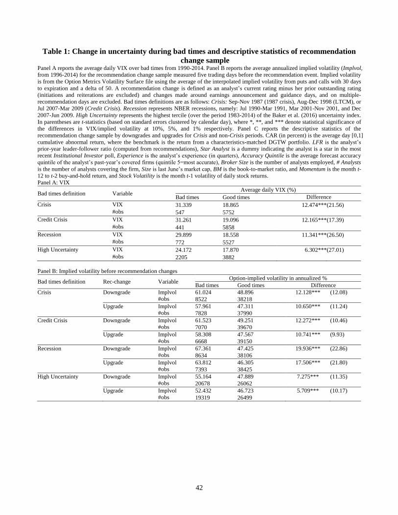
42

Table 1: Change in uncertainty during bad times and descriptive statistics of recommendation

change sample Panel A reports the average daily VIX over bad times from 1990-2014. Panel B reports the average annualized implied volatility (Implvol,

from 1996-2014) for the recommendation change sample measured five trading days before the recommendation event. Implied volatility

is from the Option Metrics Volatility Surface file using the average of the interpolated implied volatility from puts and calls with 30 days

to expiration and a delta of 50. A recommendation change is defined as an analyst’s current rating minus her prior outstanding rating

(initiations and reiterations are excluded) and changes made around earnings announcement and guidance days, and on multiple-

recommendation days are excluded. Bad times definitions are as follows: Crisis: Sep-Nov 1987 (1987 crisis), Aug-Dec 1998 (LTCM), or

Jul 2007-Mar 2009 (Credit Crisis). Recession represents NBER recessions, namely: Jul 1990-Mar 1991, Mar 2001-Nov 2001, and Dec

2007-Jun 2009. High Uncertainty represents the highest tercile (over the period 1983-2014) of the Baker et al. (2016) uncertainty index.

In parentheses are t-statistics (based on standard errors clustered by calendar day), where *, **, and *** denote statistical significance of

the differences in VIX/implied volatility at 10%, 5%, and 1% respectively. Panel C reports the descriptive statistics of the

recommendation change sample by downgrades and upgrades for Crisis and non-Crisis periods. CAR (in percent) is the average day [0,1]

cumulative abnormal return, where the benchmark is the return from a characteristics-matched DGTW portfolio. LFR is the analyst’s

prior-year leader-follower ratio (computed from recommendations), Star Analyst is a dummy indicating the analyst is a star in the most

recent Institutional Investor poll, Experience is the analyst’s experience (in quarters), Accuracy Quintile is the average forecast accuracy

quintile of the analyst’s past-year’s covered firms (quintile 5=most accurate), Broker Size is the number of analysts employed, # Analysts

is the number of analysts covering the firm, Size is last June’s market cap, BM is the book-to-market ratio, and Momentum is the month t-

12 to t-2 buy-and-hold return, and Stock Volatility is the month t-1 volatility of daily stock returns.

Panel A: VIX

Bad times definition Variable Average daily VIX (%)

Bad times Good times Difference

Crisis VIX 31.339 18.865 12.474*** (21.56)

#obs 547 5752 Credit Crisis VIX 31.261 19.096 12.165*** (17.39)

#obs 441 5858 Recession VIX 29.899 18.558 11.341*** (26.50)

#obs 772 5527

High Uncertainty VIX 24.172 17.870 6.302*** (27.01)

#obs 2205 3882

Panel B: Implied volatility before recommendation changes

Bad times definition Rec-change Variable Option-implied volatility in annualized %

Bad times Good times Difference

Crisis Downgrade Implvol 61.024 48.896 12.128*** (12.08)

#obs 8522 38218

Upgrade Implvol 57.961 47.311 10.650*** (11.24)

#obs 7828 37990

Credit Crisis Downgrade Implvol 61.523 49.251 12.272*** (10.46)

#obs 7070 39670

Upgrade Implvol 58.308 47.567 10.741*** (9.93)

#obs 6668 39150

Recession Downgrade Implvol 67.361 47.425 19.936*** (22.86)

#obs 8634 38106

Upgrade Implvol 63.812 46.305 17.506*** (21.80)

#obs 7393 38425

High Uncertainty Downgrade Implvol 55.164 47.889 7.275*** (11.35)

#obs 20678 26062

Upgrade Implvol 52.432 46.723 5.709*** (10.17)

#obs 19319 26499

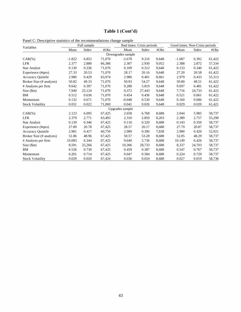
43

Table 1 (Cont’d)

Panel C: Descriptive statistics of the recommendations change sample

Variables Full sample Bad times: Crisis periods Good times: Non-Crisis periods

Mean Stdev #Obs Mean Stdev #Obs Mean Stdev #Obs

Downgrades sample

CAR(%) -1.822 6.852 71,070 -2.678 9.216 9,648 -1.687 6.392 61,422

LFR 2.377 2.880 66,386 2.307 2.930 9,052 2.388 2.872 57,334

Star Analyst 0.130 0.336 71,070 0.109 0.312 9,648 0.133 0.340 61,422

Experience (#qtrs) 27.33 20.53 71,070 28.17 20.16 9,648 27.20 20.58 61,422

Accuracy Quintile 2.980 0.429 63,974 2.986 0.401 8,661 2.979 0.433 55,313

Broker Size (# analysts) 50.82 49.33 71,070 50.93 54.27 9,648 50.80 48.51 61,422

# Analysts per firm 9.642 6.397 71,070 9.288 5.819 9,648 9.697 6.481 61,422

Size ($m) 7,940 25,124 71,070 9,372 27,443 9,648 7,716 24,733 61,422

BM 0.512 0.636 71,070 0.454 0.436 9,648 0.521 0.661 61,422

Momentum 0.132 0.671 71,070 -0.048 0.530 9,648 0.160 0.686 61,422

Stock Volatility 0.031 0.022 71,069 0.041 0.026 9,648 0.029 0.020 61,421

Upgrades sample

CAR(%) 2.123 6.095 67,425 2.658 6.768 8,688 2.044 5.985 58,737

LFR 2.379 2.771 63,493 2.310 2.859 8,203 2.389 2.757 55,290

Star Analyst 0.139 0.346 67,425 0.116 0.320 8,688 0.143 0.350 58,737

Experience (#qtrs) 27.89 20.78 67,425 28.57 20.17 8,688 27.79 20.87 58,737

Accuracy Quintile 2.981 0.417 60,759 2.989 0.390 7,838 2.980 0.420 52,921

Broker Size (# analysts) 51.86 48.96 67,425 50.57 53.28 8,688 52.05 48.29 58,737

# Analysts per firm 10.083 6.344 67,425 9.640 5.736 8,688 10.149 6.426 58,737

Size ($m) 8,591 25,266 67,425 10,306 28,733 8,688 8,337 24,703 58,737

BM 0.536 0.730 67,425 0.459 0.387 8,688 0.547 0.767 58,737

Momentum 0.201 0.714 67,425 0.047 0.584 8,688 0.224 0.729 58,737

Stock Volatility 0.029 0.020 67,424 0.036 0.024 8,688 0.027 0.019 58,736

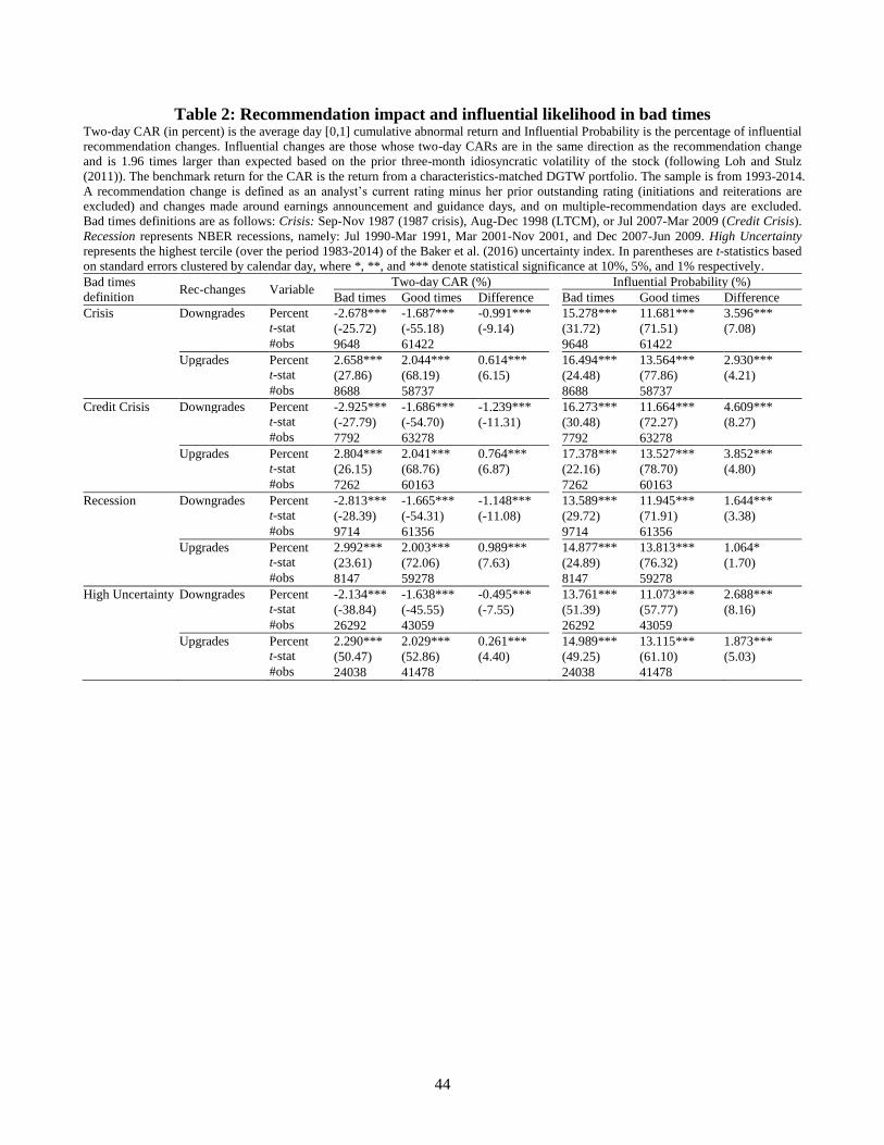
44

Table 2: Recommendation impact and influential likelihood in bad times Two-day CAR (in percent) is the average day [0,1] cumulative abnormal return and Influential Probability is the percentage of influential

recommendation changes. Influential changes are those whose two-day CARs are in the same direction as the recommendation change

and is 1.96 times larger than expected based on the prior three-month idiosyncratic volatility of the stock (following Loh and Stulz

(2011)). The benchmark return for the CAR is the return from a characteristics-matched DGTW portfolio. The sample is from 1993-2014.

A recommendation change is defined as an analyst’s current rating minus her prior outstanding rating (initiations and reiterations are

excluded) and changes made around earnings announcement and guidance days, and on multiple-recommendation days are excluded.

Bad times definitions are as follows: Crisis: Sep-Nov 1987 (1987 crisis), Aug-Dec 1998 (LTCM), or Jul 2007-Mar 2009 (Credit Crisis).

Recession represents NBER recessions, namely: Jul 1990-Mar 1991, Mar 2001-Nov 2001, and Dec 2007-Jun 2009. High Uncertainty

represents the highest tercile (over the period 1983-2014) of the Baker et al. (2016) uncertainty index. In parentheses are t-statistics based

on standard errors clustered by calendar day, where *, **, and *** denote statistical significance at 10%, 5%, and 1% respectively.

Bad times

definition Rec-changes Variable

Two-day CAR (%) Influential Probability (%)

Bad times Good times Difference Bad times Good times Difference

Crisis Downgrades Percent -2.678*** -1.687*** -0.991*** 15.278*** 11.681*** 3.596***

t-stat (-25.72) (-55.18) (-9.14) (31.72) (71.51) (7.08)

#obs 9648 61422 9648 61422

Upgrades Percent 2.658*** 2.044*** 0.614*** 16.494*** 13.564*** 2.930***

t-stat (27.86) (68.19) (6.15) (24.48) (77.86) (4.21)

#obs 8688 58737 8688 58737

Credit Crisis Downgrades Percent -2.925*** -1.686*** -1.239*** 16.273*** 11.664*** 4.609***

t-stat (-27.79) (-54.70) (-11.31) (30.48) (72.27) (8.27)

#obs 7792 63278 7792 63278

Upgrades Percent 2.804*** 2.041*** 0.764*** 17.378*** 13.527*** 3.852***

t-stat (26.15) (68.76) (6.87) (22.16) (78.70) (4.80)

#obs 7262 60163 7262 60163

Recession Downgrades Percent -2.813*** -1.665*** -1.148*** 13.589*** 11.945*** 1.644***

t-stat (-28.39) (-54.31) (-11.08) (29.72) (71.91) (3.38)

#obs 9714 61356 9714 61356

Upgrades Percent 2.992*** 2.003*** 0.989*** 14.877*** 13.813*** 1.064*

t-stat (23.61) (72.06) (7.63) (24.89) (76.32) (1.70)

#obs 8147 59278 8147 59278

High Uncertainty Downgrades Percent -2.134*** -1.638*** -0.495*** 13.761*** 11.073*** 2.688*** t-stat (-38.84) (-45.55) (-7.55) (51.39) (57.77) (8.16)

#obs 26292 43059 26292 43059

Upgrades Percent 2.290*** 2.029*** 0.261*** 14.989*** 13.115*** 1.873***

t-stat (50.47) (52.86) (4.40) (49.25) (61.10) (5.03)

#obs 24038 41478 24038 41478

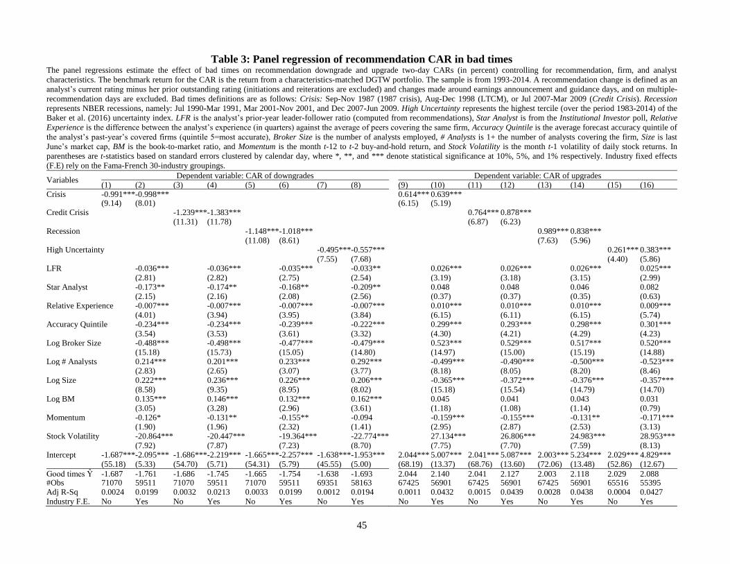
45

Table 3: Panel regression of recommendation CAR in bad times The panel regressions estimate the effect of bad times on recommendation downgrade and upgrade two-day CARs (in percent) controlling for recommendation, firm, and analyst

characteristics. The benchmark return for the CAR is the return from a characteristics-matched DGTW portfolio. The sample is from 1993-2014. A recommendation change is defined as an

analyst’s current rating minus her prior outstanding rating (initiations and reiterations are excluded) and changes made around earnings announcement and guidance days, and on multiple-

recommendation days are excluded. Bad times definitions are as follows: Crisis: Sep-Nov 1987 (1987 crisis), Aug-Dec 1998 (LTCM), or Jul 2007-Mar 2009 (Credit Crisis). Recession

represents NBER recessions, namely: Jul 1990-Mar 1991, Mar 2001-Nov 2001, and Dec 2007-Jun 2009. High Uncertainty represents the highest tercile (over the period 1983-2014) of the

Baker et al. (2016) uncertainty index. LFR is the analyst’s prior-year leader-follower ratio (computed from recommendations), Star Analyst is from the Institutional Investor poll, Relative

Experience is the difference between the analyst’s experience (in quarters) against the average of peers covering the same firm, Accuracy Quintile is the average forecast accuracy quintile of

the analyst’s past-year’s covered firms (quintile 5=most accurate), Broker Size is the number of analysts employed, # Analysts is 1+ the number of analysts covering the firm, Size is last

June’s market cap, BM is the book-to-market ratio, and Momentum is the month t-12 to t-2 buy-and-hold return, and Stock Volatility is the month t-1 volatility of daily stock returns. In

parentheses are t-statistics based on standard errors clustered by calendar day, where *, **, and *** denote statistical significance at 10%, 5%, and 1% respectively. Industry fixed effects

(F.E) rely on the Fama-French 30-industry groupings.

Variables Dependent variable: CAR of downgrades Dependent variable: CAR of upgrades

(1) (2) (3) (4) (5) (6) (7) (8) (9) (10) (11) (12) (13) (14) (15) (16) Crisis -0.991*** -0.998*** 0.614*** 0.639*** (9.14) (8.01) (6.15) (5.19) Credit Crisis -1.239*** -1.383*** 0.764*** 0.878*** (11.31) (11.78) (6.87) (6.23) Recession -1.148*** -1.018*** 0.989*** 0.838*** (11.08) (8.61) (7.63) (5.96) High Uncertainty -0.495*** -0.557*** 0.261*** 0.383*** (7.55) (7.68) (4.40) (5.86) LFR -0.036*** -0.036*** -0.035*** -0.033** 0.026*** 0.026*** 0.026*** 0.025*** (2.81) (2.82) (2.75) (2.54) (3.19) (3.18) (3.15) (2.99) Star Analyst -0.173** -0.174** -0.168** -0.209** 0.048 0.048 0.046 0.082

(2.15) (2.16) (2.08) (2.56) (0.37) (0.37) (0.35) (0.63) Relative Experience -0.007*** -0.007*** -0.007*** -0.007*** 0.010*** 0.010*** 0.010*** 0.009*** (4.01) (3.94) (3.95) (3.84) (6.15) (6.11) (6.15) (5.74) Accuracy Quintile -0.234*** -0.234*** -0.239*** -0.222*** 0.299*** 0.293*** 0.298*** 0.301*** (3.54) (3.53) (3.61) (3.32) (4.30) (4.21) (4.29) (4.23) Log Broker Size -0.488*** -0.498*** -0.477*** -0.479*** 0.523*** 0.529*** 0.517*** 0.520*** (15.18) (15.73) (15.05) (14.80) (14.97) (15.00) (15.19) (14.88) Log # Analysts 0.214*** 0.201*** 0.233*** 0.292*** -0.499*** -0.490*** -0.500*** -0.523*** (2.83) (2.65) (3.07) (3.77) (8.18) (8.05) (8.20) (8.46) Log Size 0.222*** 0.236*** 0.226*** 0.206*** -0.365*** -0.372*** -0.376*** -0.357*** (8.58) (9.35) (8.95) (8.02) (15.18) (15.54) (14.79) (14.70) Log BM 0.135*** 0.146*** 0.132*** 0.162*** 0.045 0.041 0.043 0.031 (3.05) (3.28) (2.96) (3.61) (1.18) (1.08) (1.14) (0.79) Momentum -0.126* -0.131** -0.155** -0.094 -0.159*** -0.155*** -0.131** -0.171*** (1.90) (1.96) (2.32) (1.41) (2.95) (2.87) (2.53) (3.13) Stock Volatility -20.864*** -20.447*** -19.364*** -22.774*** 27.134*** 26.806*** 24.983*** 28.953*** (7.92) (7.87) (7.23) (8.70) (7.75) (7.70) (7.59) (8.13) Intercept -1.687*** -2.095*** -1.686*** -2.219*** -1.665*** -2.257*** -1.638*** -1.953*** 2.044*** 5.007*** 2.041*** 5.087*** 2.003*** 5.234*** 2.029*** 4.829*** (55.18) (5.33) (54.70) (5.71) (54.31) (5.79) (45.55) (5.00) (68.19) (13.37) (68.76) (13.60) (72.06) (13.48) (52.86) (12.67)

Good times Ŷ -1.687 -1.761 -1.686 -1.745 -1.665 -1.754 -1.638 -1.693 2.044 2.140 2.041 2.127 2.003 2.118 2.029 2.088 #Obs 71070 59511 71070 59511 71070 59511 69351 58163 67425 56901 67425 56901 67425 56901 65516 55395 Adj R-Sq 0.0024 0.0199 0.0032 0.0213 0.0033 0.0199 0.0012 0.0194 0.0011 0.0432 0.0015 0.0439 0.0028 0.0438 0.0004 0.0427 Industry F.E. No Yes No Yes No Yes No Yes No Yes No Yes No Yes No Yes

46

Table 4: Probit of recommendation influential probability in bad times The probit regressions estimate the marginal effect (in percent) of bad times on the influential probability of the CAR for recommendation changes controlling for recommendation,

firm, and analyst characteristics. Influential changes are those whose two-day CARs are in the same direction as the recommendation change and is 1.96 times larger than expected

based on the prior three-month idiosyncratic volatility of the stock (following Loh and Stulz (2011)). The sample is from 1993-2014. A recommendation change is defined as an

analyst’s current rating minus her prior outstanding rating (initiations and reiterations are excluded) and changes made around earnings announcement days and on earnings

guidance days, and on multiple-recommendation days are excluded. Bad times definitions are as follows: Crisis: Sep-Nov 1987 (1987 crisis), Aug-Dec 1998 (LTCM), or Jul 2007-

Mar 2009 (Credit Crisis). Recession represents NBER recessions, namely: Jul 1990-Mar 1991, Mar 2001-Nov 2001, and Dec 2007-Jun 2009. High Uncertainty represents the

highest tercile (over the period 1983-2014) of the Baker et al. (2016) uncertainty index. LFR is the analyst’s prior-year leader-follower ratio (computed from recommendations),

Star Analyst is from the Institutional Investor poll, Relative Experience is the difference between the analyst’s experience (in quarters) against the average of peers covering the

same firm, Accuracy Quintile is the average forecast accuracy quintile of the analyst’s past-year’s covered firms (quintile 5=most accurate), Broker Size is the number of analysts

employed, # Analysts is 1+ the number of analysts covering the firm, Size is last June’s market cap, BM is the book-to-market ratio, and Momentum is the month t-12 to t-2 buy-

and-hold return, and Stock Volatility is the month t-1 volatility of daily stock returns. In parentheses are z-statistics based on standard errors clustered by calendar day, where *, **,

and *** denote statistical significance at 10%, 5%, and 1% respectively. Industry fixed effects rely on the Fama-French 30-industry groupings.

Variables Dependent variable: Influential dummy for downgrades Dependent variable: Influential dummy for upgrades

(1) (2) (3) (4) (5) (6) (7) (8)

(9) (10) (11) (12) (13) (14) (15) (16) Crisis 0.036*** 0.065*** 0.029*** 0.055*** (7.56) (12.02) (4.45) (8.03) Credit Crisis 0.046*** 0.079*** 0.039*** 0.067*** (9.00) (13.30) (5.15) (8.60) Recession 0.016*** 0.048*** 0.011* 0.042*** (3.49) (8.65) (1.74) (6.29)

High Uncertainty 0.027*** 0.040*** 0.019*** 0.032*** (8.30) (11.50) (5.09) (8.31) LFR 0.001*** 0.001*** 0.001*** 0.001*** 0.001** 0.001** 0.001** 0.001** (3.42) (3.42) (3.35) (3.02) (2.50) (2.47) (2.46) (2.27) Star Analyst -0.002 -0.002 -0.003 0.000 -0.014*** -0.014*** -0.014*** -0.012***

(0.52) (0.51) (0.67) (0.06) (3.04) (3.03) (3.14) (2.63) Relative Experience 0.000*** 0.000*** 0.000*** 0.000*** 0.001*** 0.001*** 0.001*** 0.001***

(4.46) (4.41) (4.44) (3.77) (6.86) (6.86) (6.90) (5.71) Accuracy Quintile 0.018*** 0.018*** 0.019*** 0.017*** 0.015*** 0.015*** 0.015*** 0.016*** (5.56) (5.58) (5.65) (5.19) (4.20) (4.12) (4.25) (4.49) Log Broker Size 0.030*** 0.030*** 0.030*** 0.029*** 0.034*** 0.035*** 0.034*** 0.034*** (19.61) (19.85) (19.14) (18.76) (19.73) (19.82) (19.48) (19.71) Log # Analysts -0.006*** -0.007*** -0.006*** -0.006*** -0.051*** -0.050*** -0.052*** -0.051*** (5.12) (5.41) (4.77) (4.76) (15.12) (15.05) (15.32) (15.02) Log Size -0.006*** -0.007*** -0.006*** -0.006*** -0.012*** -0.012*** -0.012*** -0.012*** (5.12) (5.41) (4.77) (4.76) (8.84) (9.09) (8.46) (8.31) Log BM -0.005*** -0.005*** -0.005*** -0.007*** 0.002 0.002 0.002 0.001 (2.70) (2.95) (2.72) (3.64) (1.13) (1.01) (0.98) (0.26) Momentum 0.008*** 0.008*** 0.008*** 0.007*** -0.007** -0.006** -0.006** -0.007***

(3.77) (3.77) (3.93) (3.17) (2.49) (2.45) (2.37) (2.82) Stock Volatility -1.288*** -1.273*** -1.296*** -1.182*** -1.704*** -1.700*** -1.729*** -1.550*** (13.25) (13.22) (12.98) (12.23) (13.47) (13.48) (13.85) (12.28)

Predicted Prob. 0.121 0.117 0.121 0.117 0.122 0.118 0.120 0.117 0.139 0.134 0.139 0.134 0.139 0.135 0.138 0.134 #Obs 71070 59511 71070 59511 71070 59511 69351 58163 67425 56901 67425 56901 67425 56901 65516 55395 Industry F.E. No Yes No Yes No Yes No Yes No Yes No Yes No Yes No Yes

47

Table 5: Panel regression of forecast revision CAR in bad times The panel regressions estimate the effect of bad times on earnings forecast revisions two-day CARs (in percent) controlling for forecast, firm, and analyst characteristics. The

benchmark return for the CAR is the return from a characteristics-matched DGTW portfolio. The sample is from 1983-2014. Forecast Revision is the analyst’s current one-quarter-

ahead earnings forecast minus her prior outstanding forecast (i.e., initiations are excluded) scaled by price and revisions made around earnings announcement and guidance days,

and on multiple-forecast days are excluded. Bad times definitions are as follows: Crisis: Sep-Nov 1987 (1987 crisis), Aug-Dec 1998 (LTCM), or Jul 2007-Mar 2009 (Credit

Crisis). Recession represents NBER recessions, namely: Jul 1990-Mar 1991, Mar 2001-Nov 2001, and Dec 2007-Jun 2009. High Uncertainty represents the highest tercile (over

the period 1983-2014) of the Baker et al. (2016) uncertainty index. Other controls are as defined in Table 3. In parentheses are t-statistics based on standard errors clustered by

calendar day, where *, **, and *** denote statistical significance at 10%, 5%, and 1% respectively. Industry fixed effects (F.E.) rely on the Fama-French 30-industry groupings.

Variables Dependent variable: CAR of downward revisions Dependent variable: CAR of upward revisions

(1) (2) (3) (4) (5) (6) (7) (8) (9) (10) (11) (12) (13) (14) (15) (16) Crisis -0.398*** -0.384*** 0.198*** 0.170** (6.50) (5.49) (2.79) (2.13) Credit Crisis -0.525*** -0.533*** 0.211*** 0.169* (7.91) (7.14) (2.68) (1.96) Recession -0.323*** -0.238*** 0.108 0.019 (5.87) (3.50) (1.55) (0.23) High Uncertainty -0.070** -0.095*** 0.021 0.013 (2.31) (2.79) (0.70) (0.39) Forecast Revision 6.865* 6.785* 6.855* 6.547* 9.306 9.214 9.548 8.969

(1.81) (1.79) (1.81) (1.72) (1.18) (1.17) (1.21) (1.12) LFR -0.025*** -0.024*** -0.026*** -0.027*** 0.040*** 0.040*** 0.041*** 0.042*** (4.31) (4.17) (4.56) (4.61) (6.05) (6.03) (6.12) (6.18) Star Analyst 0.025 0.021 0.034 0.035 -0.093*** -0.094*** -0.097*** -0.098***

(0.76) (0.65) (1.03) (1.04) (2.67) (2.68) (2.78) (2.69) Relative Experience -0.001 -0.001 -0.001 -0.001 0.001 0.001 0.001 0.001 (0.87) (0.88) (0.88) (1.04) (0.72) (0.72) (0.75) (0.61) Accuracy Quintile -0.015 -0.015 -0.014 -0.004 0.040 0.040 0.039 0.037 (0.55) (0.58) (0.54) (0.17) (1.45) (1.45) (1.42) (1.29) Log Broker Size -0.057*** -0.057*** -0.058*** -0.067*** 0.052*** 0.052*** 0.053*** 0.050*** (3.30) (3.32) (3.38) (3.75) (2.86) (2.86) (2.92) (2.68) Log # Analysts 0.096** 0.092** 0.108*** 0.134*** -0.076* -0.079* -0.087** -0.093** (2.31) (2.22) (2.59) (3.10) (1.78) (1.85) (2.06) (2.09) Log Size 0.033** 0.039*** 0.028** 0.019 -0.075*** -0.075*** -0.070*** -0.070*** (2.34) (2.75) (1.98) (1.28) (5.18) (5.15) (4.84) (4.69) Log BM -0.019 -0.016 -0.018 -0.019 0.012 0.011 0.010 0.015 (0.85) (0.73) (0.81) (0.83) (0.53) (0.51) (0.43) (0.63) Momentum 0.040 0.034 0.043 0.069 0.073** 0.072** 0.067* 0.063* (0.94) (0.80) (0.98) (1.56) (2.04) (2.03) (1.86) (1.75) Stock Volatility -1.036 -0.438 -1.506 -3.383 4.416* 4.537* 5.057** 5.295** (0.46) (0.20) (0.64) (1.51) (1.88) (1.94) (2.09) (2.23) Intercept -0.294*** -0.646*** -0.288*** -0.717*** -0.296*** -0.598*** -0.323*** -0.465** 0.439*** 1.234*** 0.441*** 1.231*** 0.447*** 1.184*** 0.453*** 1.205*** (20.46) (3.00) (20.06) (3.36) (20.35) (2.76) (19.78) (2.14) (31.41) (5.34) (31.68) (5.33) (32.34) (5.12) (24.25) (5.10)

Good times Ŷ -0.294 -0.230 -0.288 -0.220 -0.296 -0.243 -0.323 -0.244 0.439 0.413 0.441 0.415 0.447 0.427 0.453 0.426 #Obs 172482 105097 172482 105097 172482 105097 164257 99663 112149 69773 112149 69773 112149 69773 107047 66470 Adj R-Sq 0.0009 0.0030 0.0013 0.0036 0.0007 0.0024 0.0001 0.0022 0.0002 0.0053 0.0002 0.0052 0.0001 0.0051 -0.0000 0.0051 Industry F.E. No Yes No Yes No Yes No Yes No Yes No Yes No Yes No Yes

48

Table 6: Probit of forecast revision influential probability in bad times The probit regressions estimate the marginal effect (in percent) of bad times on the influential probability of the CAR for earnings forecast revisions controlling for forecast, firm,

and analyst characteristics. Influential revisions are those whose two-day CARs are in the same direction as the revision and is 1.96 times larger than expected based on the prior

three-month idiosyncratic volatility of the stock (following Loh and Stulz (2011)). The sample is from 1983-2014. Forecast Revision is the analyst’s current one-quarter-ahead

earnings forecast minus her prior outstanding forecast (i.e., initiations are excluded) scaled by price and revisions made around earnings announcement and guidance days, and on

multiple-forecast days are excluded. Bad times definitions are as follows: Crisis: Sep-Nov 1987 (1987 crisis), Aug-Dec 1998 (LTCM), or Jul 2007-Mar 2009 (Credit Crisis).

Recession represents NBER recessions, namely: Jul 1990-Mar 1991, Mar 2001-Nov 2001, and Dec 2007-Jun 2009. High Uncertainty represents the highest tercile (over the period

1983-2014) of the Baker et al. (2016) uncertainty index. Forecast Revision is analyst’s current forecast minus her prior forecast, scaled by the stock price. Other controls are as

defined in Table 3. In parentheses are z-statistics based on standard errors clustered by calendar day, where *, **, and *** denote statistical significance at 10%, 5%, and 1%

respectively. Industry fixed effects (F.E.) rely on the Fama-French 30-industry groupings.

Variables Dependent variable: Influential dummy for downward revisions Dependent variable: Influential dummy for upward revisions

(1) (2) (3) (4) (5) (6) (7) (8)

(9) (10) (11) (12) (13) (14) (15) (16)

Crisis 0.025*** 0.036*** 0.017*** 0.024***

(8.89) (10.96) (5.85) (6.57)

Credit Crisis 0.029*** 0.042*** 0.020*** 0.025***

(9.25) (11.51) (6.28) (6.43)

Recession 0.016*** 0.028*** 0.005* 0.010***

(6.16) (8.82) (1.77) (2.63)

High Uncertainty 0.011*** 0.016*** 0.004** 0.006***

(7.00) (9.28) (2.57) (2.77)

Forecast Revision -0.340*** -0.334*** -0.338*** -0.321*** 0.740*** 0.725*** 0.746*** 0.676**

(4.48) (4.43) (4.43) (4.17) (2.70) (2.65) (2.72) (2.41)

LFR 0.001*** 0.001*** 0.001*** 0.001*** 0.001*** 0.001*** 0.001*** 0.001***

(4.83) (4.71) (5.42) (5.96) (4.92) (4.86) (5.11) (5.27)

Star Analyst -0.000 -0.000 -0.001 -0.000 -0.001 -0.001 -0.002 -0.002

(0.17) (0.13) (0.61) (0.05) (0.61) (0.60) (0.83) (0.67)

Relative Experience 0.000 0.000 0.000 0.000 0.000 0.000 0.000 0.000

(0.60) (0.64) (0.58) (0.69) (1.19) (1.20) (1.25) (1.33)

Accuracy Quintile 0.002 0.002 0.002 0.001 0.003* 0.003* 0.003* 0.003*

(1.36) (1.40) (1.43) (0.71) (1.92) (1.93) (1.91) (1.76)

Log Broker Size 0.003*** 0.003*** 0.003*** 0.004*** 0.004*** 0.004*** 0.004*** 0.004***

(3.92) (4.00) (4.04) (4.64) (4.07) (4.06) (4.16) (3.93)

Log # Analysts -0.001* -0.001** -0.001 -0.001 -0.015*** -0.015*** -0.016*** -0.018***

(1.90) (2.05) (1.54) (0.73) (5.77) (5.87) (6.19) (6.43)

Log Size -0.001* -0.001** -0.001 -0.001 -0.003*** -0.003*** -0.003*** -0.002**

(1.90) (2.05) (1.54) (0.73) (3.57) (3.51) (3.02) (2.48)

Log BM -0.001 -0.002* -0.002 -0.002** -0.003** -0.003** -0.003** -0.003**

(1.45) (1.67) (1.59) (2.34) (2.25) (2.28) (2.47) (2.54)

Momentum 0.005*** 0.005*** 0.005*** 0.002 0.001 0.001 0.001 0.000

(3.54) (3.52) (3.75) (1.41) (0.68) (0.66) (0.41) (0.08)

Stock Volatility -0.501*** -0.504*** -0.501*** -0.326*** -0.601*** -0.588*** -0.557*** -0.480***

(7.44) (7.61) (7.16) (4.77) (7.24) (7.15) (6.62) (5.83)

Predicted Prob. 0.049 0.045 0.049 0.045 0.049 0.045 0.048 0.044 0.053 0.050 0.053 0.050 0.053 0.050 0.053 0.051

#Obs 172481 105097 172481 105097 172481 105097 164256 99663 112147 69773 112147 69773 112147 69773 107045 66470

Industry F.E. No Yes No Yes No Yes No Yes No Yes No Yes No Yes No Yes

49

Table 7: Robustness tests Panel A estimates the effect of high firm, industry, and market uncertainty on the two-day CAR (in percent) of recommendation changes. Control variables are estimated for even

specifications but not reported (see Table 3 for definitions of controls). A firm’s total variance of daily stock returns in the prior month is decomposed into a market, industry, and firm

part by regressing daily returns on market returns and a market-purged industry return (Fama-French 30 industry groups). High uncertainty equals one when the relevant component is in

the top tercile within the firm’s time-series of monthly variance components. Panel B estimates the effect of bad times on the two-day CARs (in percent) of recommendation reiterations.

The benchmark return for the CAR is the return from a characteristics-matched DGTW portfolio. The sample is from 1993-2014. A recommendation reiteration is either an explicit

reiteration from the I/B/E/S recommendation file, or an assumed reiteration that the analyst’s outstanding rating is reiterated when there is a quarterly earnings or target price forecast

with no new rating issued. Control variables (in even specifications but unreported) are the same as those in Table 3 plus forecast revision over price and target price over current price

when available or zero otherwise. Reiterations made around earnings announcement and guidance days and on multiple-reiteration days are excluded. Bad times definitions are as

follows: Crisis: Sep-Nov 1987 (1987 crisis), Aug-Dec 1998 (LTCM), or Jul 2007-Mar 2009 (Credit Crisis). Recession represents NBER recessions, namely: Jul 1990-Mar 1991, Mar

2001-Nov 2001, and Dec 2007-Jun 2009. High Uncertainty represents the highest tercile (over the period 1983-2014) of the Baker et al. (2016) uncertainty index. Panel C regresses the

daily absolute returns of firms in the CRSP file from 1993-2014 on firm news event dummies and bad times dummies, excluding observations where the lagged price is less than one

dollar. Event dummies equals one for day 0 of the announcement, or day 1 if the announcement occurs after trading hours (checking when we have the time stamps). Earnings

announcement dates are from Compustat and times from I/B/E/S, guidance events are from First Call Guidelines (I/B/E/S Guidance from 2011 onwards), dividend events are from the

CRSP event file, and insider trade events are from the Thomson Insider Form 4 file. Size, BM, and Momentum are as defined in Table 3. Other control variables Lag Return, Idio.

Volatility, Turnover, and Inst. Ownership are measured in the prior month. In parentheses are t-statistics based on standard errors clustered by calendar day, where *, **, and *** denote

statistical significance at 10%, 5%, and 1% respectively. Industry fixed effects (F.E.) rely on the Fama-French 30-industry groupings.

Panel A: Panel regression of recommendation change CAR on different measures of high uncertainty

Variables Dependent variable: CAR of downgrades

Dependent variable: CAR of upgrades

(1) (2) (3) (4) (5) (6) (7) (8) (9) (10) (11) (12) (13) (14) (15) (16) High Firm Uncertainty -1.091*** 0.149 -0.932*** 0.061 1.707*** 0.266* 1.618*** 0.347** (11.64) (1.08) (9.93) (0.44) (16.32) (1.86) (15.28) (2.44) High Ind. Uncertainty -0.297*** -0.004 0.001 0.012 0.143*** 0.020 -0.199*** 0.012

(5.29) (0.07) (0.02) (0.18) (2.69) (0.30) (3.90) (0.19) High Mkt Uncertainty -0.783*** -0.501*** -0.622*** -0.497*** 0.757*** 0.379*** 0.555*** 0.404*** (13.77) (6.81) (10.71) (6.63) (14.60) (5.01) (9.90) (5.20)

Good times Ŷ -1.590 -1.928 -1.703 -1.895 -1.471 -1.670 -1.345 -1.689 1.820 2.176 2.067 2.214 1.786 2.051 1.667 1.975 Observations 71067 59510 71067 59510 71067 59510 71067 59510 67424 56901 67424 56901 67424 56901 67424 56901 Adj R-Sq 0.0042 0.0177 0.0004 0.0176 0.0032 0.0187 0.0061 0.0186 0.0114 0.0422 0.0001 0.0421 0.0038 0.0428 0.0134 0.0430 Controls, Ind F.E. No Yes No Yes No Yes No Yes No Yes No Yes No Yes No Yes

Panel B: Panel regression of reiteration CAR in bad times

Variables Dependent variable: CAR of unfavorable recommendation reiterations Dependent variable: CAR of favorable recommendation reiterations

(1) (2) (3) (4) (5) (6) (7) (8) (9) (10) (11) (12) (13) (14) (15) (16) Crisis -0.262*** -0.173*** -0.163*** -0.105** (5.72) (3.78) (3.52) (2.39) Credit Crisis -0.293*** -0.215*** -0.163*** -0.110**

(6.02) (4.45) (3.12) (2.21)

Recession -0.252*** -0.164*** -0.167*** -0.131*** (5.36) (3.42) (3.83) (3.06) High Uncertainty -0.090*** -0.100*** -0.021 -0.029

(3.79) (4.23) (0.91) (1.29)

Non-bad times Ŷ -0.064 -0.076 -0.064 -0.073 -0.065 -0.077 -0.060 -0.056 0.175 0.166 0.171 0.164 0.178 0.171 0.164 0.164 Observations 248676 243190 248676 243190 248676 243190 237063 231964 347922 339883 347922 339883 347922 339883 334452 326827 Adj R-Sq 0.0004 0.0024 0.0005 0.0024 0.0004 0.0023 0.0001 0.0023 0.0001 0.0023 0.0001 0.0023 0.0001 0.0023 0.0000 0.0023 Controls, Ind. F.E. No Yes No Yes No Yes No Yes No Yes No Yes No Yes No Yes

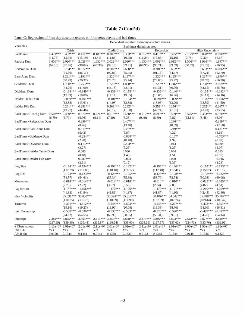
50

Table 7 (Cont’d)

Panel C: Regression of firm-day absolute returns on firm news events and bad times

Variables

Dependent variable: Firm-day absolute returns

Bad times definition used

Crisis Credit Crisis Recession High Uncertainty

BadTimes 0.471*** 0.432*** 0.411*** 0.185*** 0.380*** 0.353*** 0.517*** 0.416*** 0.395*** -0.179*** 0.098*** 0.090*** (11.75) (15.96) (15.19) (4.31) (11.83) (10.98) (16.24) (15.83) (15.10) (7.78) (7.30) (6.67)

Recchg Dum 1.656*** 2.020*** 2.028*** 1.652*** 2.022*** 2.030*** 1.630*** 2.002*** 2.012*** 1.506*** 1.936*** 1.947***

(67.10) (97.96) (98.84) (67.90) (99.15) (99.91) (66.95) (98.71) (99.69) (50.09) (75.37) (76.95)

Reiteration Dum 0.704*** 0.672*** 0.702*** 0.660*** 0.701*** 0.662*** 0.693*** 0.606***

(91.30) (86.11) (90.86) (85.75) (91.18) (84.57) (87.24) (62.70)

Earn Annc Dum 1.221*** 1.191*** 1.220*** 1.197*** 1.220*** 1.195*** 1.227*** 1.190***

(80.29) (76.37) (79.28) (75.44) (79.80) (75.77) (78.59) (66.90)

Guidance Dum 1.730*** 1.753*** 1.729*** 1.808*** 1.726*** 1.746*** 1.780*** 2.069***

(44.26) (41.90) (44.18) (42.41) (44.31) (40.76) (44.15) (35.78)

Dividend Dum -0.138*** -0.149*** -0.138*** -0.155*** -0.136*** -0.140*** -0.135*** -0.142***

(17.09) (18.09) (17.17) (19.05) (16.85) (16.96) (16.11) (14.16)

Insider Trade Dum -0.099*** -0.101*** -0.101*** -0.104*** -0.094*** -0.099*** -0.100*** -0.106***

(13.88) (13.61) (14.03) (13.88) (13.03) (13.20) (13.59) (11.50)

Insider File Dum 0.261*** 0.253*** 0.262*** 0.262*** 0.259*** 0.256*** 0.262*** 0.267***

(43.27) (44.46) (43.12) (41.88) (42.74) (41.01) (41.91) (35.55)

BadTimes×Recchg Dum 0.503*** 0.439*** 0.370*** 0.726*** 0.516*** 0.430*** 0.712*** 0.592*** 0.509*** 0.575*** 0.353*** 0.320***

(6.79) (6.70) (5.96) (9.11) (7.20) (6.38) (9.49) (8.69) (7.82) (12.11) (8.48) (8.06)

BadTimes×Reiteration Dum 0.259*** 0.407*** 0.296*** 0.219***

(8.46) (13.40) (10.69) (12.58)

BadTimes×Earn Annc Dum 0.319*** 0.367*** 0.249*** 0.131***

(5.43) (5.87) (4.32) (3.66)

BadTimes×Guidance Dum -0.254** -0.888*** -0.187* -0.703***

(2.20) (10.48) (1.92) (8.87)

BadTimes×Dividend Dum 0.113*** 0.203*** 0.043 0.020

(3.27) (5.28) (1.25) (1.07)

BadTimes×Insider Trade Dum 0.005 0.036 0.044 0.015

(0.18) (1.46) (1.51) (0.95)

BadTimes×Insider File Dum 0.081*** -0.003 0.030 -0.016

(2.61) (0.12) (1.36) (1.23)

Log Size -0.194*** -0.194*** -0.193*** -0.192*** -0.196*** -0.196*** -0.193*** -0.193***

(117.79) (117.83) (118.10) (118.12) (117.40) (117.41) (115.07) (115.12)

Log BM -0.123*** -0.123*** -0.125*** -0.125*** -0.128*** -0.128*** -0.132*** -0.132***

(54.57) (54.61) (55.34) (55.38) (58.79) (58.74) (60.08) (60.06)

Momentum -0.014*** -0.014*** -0.018*** -0.018*** -0.010** -0.010** -0.025*** -0.025***

(2.73) (2.72) (3.57) (3.56) (2.04) (2.03) (4.82) (4.81)

Lag Return -1.157*** -1.156*** -1.177*** -1.176*** -1.172*** -1.171*** -1.210*** -1.209***

(41.93) (41.94) (41.86) (41.87) (41.87) (41.90) (42.45) (42.46)

Idio. Volatility 35.031*** 35.030*** 35.324*** 35.317*** 34.846*** 34.842*** 35.788*** 35.787***

(110.75) (110.76) (110.89) (110.90) (107.69) (107.74) (109.44) (109.47)

Turnover -4.391*** -4.412*** -4.548*** -4.573*** -4.248*** -4.277*** -4.473*** -4.507***

(19.16) (19.27) (19.96) (20.08) (18.59) (18.76) (18.66) (18.81)

Inst. Ownership -0.530*** -0.530*** -0.533*** -0.533*** -0.520*** -0.520*** -0.497*** -0.497***

(64.62) (64.55) (68.99) (68.85) (59.34) (59.31) (54.26) (54.14)

Intercept 2.381*** 3.865*** 3.865*** 2.413*** 3.857*** 3.858*** 2.375*** 3.892*** 3.893*** 2.512*** 3.827*** 3.829***

(237.99) (139.36) (139.41) (235.87) (138.54) (138.60) (228.36) (137.57) (137.62) (224.73) (133.76) (133.92)

# Observations 2.11e+07 2.01e+07 2.01e+07 2.11e+07 2.01e+07 2.01e+07 2.11e+07 2.01e+07 2.01e+07 2.05e+07 1.95e+07 1.95e+07 Ind. F.E. Yes Yes Yes Yes Yes Yes Yes Yes Yes Yes Yes Yes

Adj R-Sq 0.0158 0.1344 0.1344 0.0144 0.1338 0.1339 0.0163 0.1343 0.1344 0.0148 0.1326 0.1327

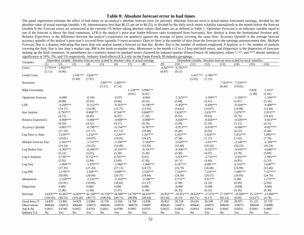
51

Table 8: Absolute forecast error in bad times The panel regressions estimate the effect of bad times on an analyst’s absolute forecast error (in percent). Absolute forecast error is actual minus forecasted earnings, divided by the

absolute value of actual earnings (models 1-8) (denominators less than $0.25 are set to $0.25), or divided by the daily stock return volatility (annualized) in the month before the forecast

(models 9-16). Forecast errors are winsorized at the extreme 1% before taking absolute values. Bad times are as defined in Table 1. Optimistic Forecast is an indicator variable equal to

one if the forecast is above the final consensus, LFR is the analyst’s prior-year leader-follower ratio (computed from forecasts), Star Analyst is from the Institutional Investor poll,

Relative Experience is the difference between the analyst’s experience (in quarters) against the average of peers covering the same firm, Accuracy Quintile is the average forecast

accuracy quintile of the analyst’s past-year’s covered firms (quintile 5=most accurate), Days to Annc is the number of days from the forecast to the earnings announcement date, Multiple

Forecast Day is a dummy indicating that more than one analyst issued a forecast on that day, Broker Size is the number of analysts employed, # Analysts is 1+ the number of analysts

covering the firm, Size is last June’s market cap, BM is the book-to-market ratio, Momentum is the month t-12 to t-2 buy-and-hold return, and Dispersion is the dispersion of forecasts

making up the final consensus. In parentheses are t-statistics based on standard errors clustered by industry-quarter (Fama-French 30 industries), where *, **, and *** denote statistical

significance at 10%, 5%, and 1% respectively. Industry fixed effects (F.E.) rely on the Fama-French 30-industry groupings.

Variables Dependent variable: Absolute forecast error scaled by absolute value of actual earnings Dependent variable: Absolute forecast error scaled by stock volatility

(1) (2) (3) (4) (5) (6) (7) (8)

(9) (10) (11) (12) (13) (14) (15) (16)

Crisis 2.775*** 2.952*** -6.667*** -6.705***

(5.11) (6.96) (6.87) (9.21)

Credit Crisis 3.341*** 3.626*** -5.417*** -5.590***

(5.49) (7.81) (5.05) (7.15)

Recession 2.807*** 2.985*** -7.933*** -7.234***

(5.11) (7.14) (8.44) (10.02)

High Uncertainty 1.128*** 0.996*** 0.828 -1.015*

(4.01) (4.41) (1.08) (1.82)

Optimistic Forecast -0.090 -0.104 -0.075 -0.064 -1.325*** -1.309*** -1.359*** -1.196***

(0.80) (0.93) (0.66) (0.55) (5.68) (5.61) (5.87) (5.16)

LFR -0.209*** -0.212*** -0.203*** -0.196*** -0.492*** -0.494*** -0.504*** -0.498***

(14.17) (14.39) (13.75) (13.03) (14.63) (14.67) (14.98) (14.44)

Star Analyst 0.793*** 0.808*** 0.764*** 0.868*** 2.620*** 2.651*** 2.679*** 2.953***

(6.72) (6.85) (6.47) (7.20) (9.52) (9.62) (9.75) (10.92)

Relative Experience -0.008*** -0.008*** -0.008*** -0.008*** -0.026*** -0.026*** -0.026*** -0.023***

(4.29) (4.31) (4.27) (4.10) (5.09) (5.10) (5.12) (4.51)

Accuracy Quintile -0.801*** -0.798*** -0.794*** -0.787*** -0.973*** -0.970*** -0.990*** -0.827***

(11.19) (11.17) (11.11) (10.68) (6.40) (6.36) (6.52) (5.44)

Log Days to Annc 1.219*** 1.232*** 1.220*** 1.207*** 1.052*** 1.024*** 1.052*** 1.095***

(19.01) (19.07) (19.05) (18.47) (7.58) (7.37) (7.63) (7.78)

Mutiple Forecast Day -1.561*** -1.551*** -1.596*** -1.569*** -2.629*** -2.637*** -2.546*** -2.549***

(14.33) (14.25) (14.49) (13.93) (10.49) (10.52) (10.23) (10.24)

Log Broker Size -0.305*** -0.300*** -0.316*** -0.335*** -0.506*** -0.522*** -0.476*** -0.640***

(5.12) (5.07) (5.20) (5.29) (3.96) (4.07) (3.78) (5.00)

Log # Analysts 0.756*** 0.752*** 0.765*** 0.415 -2.876*** -2.712*** -2.931*** -1.985***

(2.95) (2.94) (3.00) (1.50) (4.71) (4.44) (4.85) (3.33)

Log Size -1.969*** -1.979*** -1.966*** -1.886*** 4.107*** 4.081*** 4.110*** 3.630***

(27.10) (27.43) (27.13) (24.72) (16.79) (16.68) (16.99) (15.46)

Log BM 2.579*** 2.568*** 2.608*** 2.530*** 7.164*** 7.216*** 7.086*** 7.527***

(20.09) (20.04) (20.37) (18.64) (24.50) (24.57) (24.03) (24.76)

Momentum -2.259*** -2.233*** -2.104*** -2.540*** 0.775** 0.917** 0.360 1.175***

(10.91) (10.85) (10.62) (11.27) (1.99) (2.33) (0.99) (2.93)

Dispersion 0.000 0.000 0.000 0.000 -0.000 -0.000 -0.000 -0.000

(1.46) (1.46) (1.47) (1.48) (0.35) (0.32) (0.36) (0.30)

Intercept 14.835*** 45.065*** 14.829*** 45.148*** 14.759*** 44.948*** 14.700*** 44.618*** 26.852*** -16.951*** 26.616*** -17.075*** 27.199*** -16.669*** 25.123*** -13.060***

(104.43) (49.53) (105.20) (49.77) (106.84) (49.73) (90.89) (48.64) (63.64) (6.13) (63.71) (6.17) (65.12) (6.06) (53.27) (4.78)

Good times Ŷ 14.835 13.905 14.829 13.884 14.759 13.826 14.700 13.838 26.852 26.728 26.616 26.509 27.199 26.971 25.123 25.720

Observations 406644 334974 406644 334974 406644 334974 388570 318887 406642 334973 406642 334973 406642 334973 388568 318886

Adj R-Sq 0.0017 0.0786 0.0022 0.0793 0.0021 0.0789 0.0007 0.0763 0.0025 0.0824 0.0014 0.0814 0.0042 0.0833 0.0001 0.0807

Industry F.E. No Yes No Yes No Yes No Yes No Yes No Yes No Yes No Yes

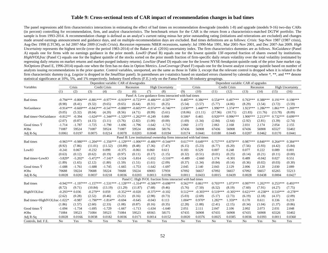
52

Table 9: Cross-sectional tests of CAR impact of recommendation changes in bad times

The panel regressions add firm characteristics interactions in estimating the effect of bad times on recommendation downgrade (models 1-8) and upgrade (models 9-16) two-day CARs

(in percent) controlling for recommendation, firm, and analyst characteristics. The benchmark return for the CAR is the return from a characteristics-matched DGTW portfolio. The

sample is from 1993-2014. A recommendation change is defined as an analyst’s current rating minus her prior outstanding rating (initiations and reiterations are excluded) and changes

made around earnings announcement and guidance days, and on multiple-recommendation days are excluded. Bad times definitions are as follows: Crisis: Sep-Nov 1987 (1987 crisis),

Aug-Dec 1998 (LTCM), or Jul 2007-Mar 2009 (Credit Crisis). Recession represents NBER recessions, namely: Jul 1990-Mar 1991, Mar 2001-Nov 2001, and Dec 2007-Jun 2009. High

Uncertainty represents the highest tercile (over the period 1983-2014) of the Baker et al. (2016) uncertainty index. The firm characteristics dummies are as follows. NoGuidance (Panel

A) equals one for firms with no earnings guidance in the prior month. LowIO (Panel B) equals one for the lowest quintile 13F-reported fraction of shares owned by institutions.

HighIVOLfrac (Panel C) equals one for the highest quintile of the stocks sorted on the prior month fraction of firm-specific daily return volatility over the total volatility (estimated by

regressing daily returns on market returns and market-purged industry returns). LowSize (Panel D) equals one for the lowest NYSE-breakpoint quintile rank of the prior June market cap.

NoOptions (Panel E, 1996-2014) equals one when the firm has no data in Option Metrics. LowCoverage (Panel F) equals one for the lowest analyst coverage quintile based on number of

analysts issuing recommendations in the prior quarter. Control variables, unreported, are the same as those in Table 3, except that the relevant control is dropped when it is related to the

firm characteristic dummy (e.g. Logsize is dropped in the SmallSize panel). In parentheses are t-statistics based on standard errors clustered by calendar day, where *, **, and *** denote

statistical significance at 10%, 5%, and 1% respectively. Industry fixed effects (F.E.) rely on the Fama-French 30-industry groupings.

Variables

Dependent variable: CAR of downgrades Dependent variable: CAR of upgrades

Crisis Credit Crisis Recession High Uncertainty Crisis Credit Crisis Recession High Uncertainty

(1) (2) (3) (4) (5) (6) (7) (8) (9) (10) (11) (12) (13) (14) (15) (16)

Panel A: Low guidance firms interacted with bad times

Bad times -0.794*** -0.806*** -0.881*** -0.977*** -0.919*** -0.723*** -0.486*** -0.507*** 0.485*** 0.386*** 0.554*** 0.497*** 0.763*** 0.388*** 0.191*** 0.198***

(8.98) (8.41) (9.32) (9.65) (9.65) (6.64) (8.31) (8.25) (5.54) (3.57) (5.77) (4.06) (8.29) (3.54) (3.72) (3.59)

NoGuidance -0.914*** -0.669*** -0.843*** -0.547*** -0.888*** -0.605*** -0.974*** -0.746*** 2.030*** 1.440*** 1.990*** 1.374*** 1.923*** 1.286*** 1.861*** 1.269***

(9.05) (5.32) (8.04) (4.20) (8.56) (4.71) (8.99) (5.61) (18.06) (11.11) (17.96) (10.71) (21.83) (11.76) (13.78) (8.09)

Bad times×NoGuidance -0.812** -0.394 -1.624*** -1.344*** -1.520*** -1.262*** -0.249 0.000 0.506* 0.465 0.920*** 0.996*** 1.900*** 2.213*** 0.732*** 0.699***

(2.07) (0.87) (4.15) (3.11) (3.76) (2.82) (1.00) (0.00) (1.69) (1.34) (2.84) (2.64) (2.92) (2.81) (3.39) (2.74)

Good times Ŷ -1.714 -1.787 -1.725 -1.790 -1.696 -1.796 -1.642 -1.712 2.060 2.172 2.063 2.168 2.031 2.174 2.054 2.155

#Obs 71087 59524 71087 59524 71087 59524 69368 58176 67436 56908 67436 56908 67436 56908 65527 55402

Adj R-Sq 0.0061 0.0197 0.0075 0.0214 0.0078 0.0203 0.0048 0.0194 0.0174 0.0441 0.0180 0.0449 0.0207 0.0462 0.0170 0.0441

Panel B: Low institutional ownership firms interacted with bad times

Bad times -0.965*** -0.980*** -1.204*** -1.356*** -1.129*** -1.006*** -0.486*** -0.544*** 0.617*** 0.649*** 0.757*** 0.879*** 0.987*** 0.840*** 0.264*** 0.384***

(8.92) (7.86) (11.01) (11.52) (10.89) (8.48) (7.36) (7.47) (6.15) (5.23) (6.77) (6.20) (7.56) (5.93) (4.42) (5.84)

LowIO -0.241 0.067 -0.232 0.099 -0.375 -0.061 0.060 0.611 0.183 0.529 0.007 0.248 0.077 0.222 0.089 0.001

(0.63) (0.12) (0.62) (0.19) (0.97) (0.11) (0.17) (1.15) (0.32) (0.51) (0.01) (0.25) (0.14) (0.21) (0.11) (0.00)

Bad times×LowIO -3.829* -5.202* -5.472** -7.141* -3.524 -5.814 -1.652 -3.516** -0.489 -2.660 1.174 -0.301 0.489 -0.042 0.027 0.551

(1.89) (1.65) (2.12) (1.80) (1.59) (1.51) (1.61) (2.09) (0.37) (1.34) (0.84) (0.14) (0.36) (0.02) (0.03) (0.30)

Good times Ŷ -1.688 -1.761 -1.688 -1.745 -1.665 -1.753 -1.642 -1.697

2.045 2.140 2.043 2.129 2.006 2.120 2.030 2.089

#Obs 70688 59224 70688 59224 70688 59224 69083 57959 67092 56657 67092 56657 67092 56657 65265 55213

Adj R-Sq 0.0028 0.0202 0.0037 0.0218 0.0036 0.0203 0.0013 0.0196 0.0011 0.0433 0.0015 0.0439 0.0028 0.0438 0.0004 0.0427

Panel C: High IVOL fraction firms interacted with bad times

Bad times -0.942*** -1.197*** -1.157*** -1.531*** -1.128*** -1.314*** -0.506*** -0.698*** 0.562*** 0.861*** 0.703*** 1.073*** 0.997*** 1.202*** 0.253*** 0.493***

(8.72) (9.71) (10.84) (13.19) (11.29) (11.87) (7.68) (9.46) (5.76) (7.50) (6.52) (8.19) (7.60) (7.91) (4.27) (7.75)

HighIVOLfrac -0.293*** 0.036 -0.279** 0.059 -0.352*** -0.020 -0.375*** -0.102 0.512*** -0.303*** 0.519*** -0.305*** 0.621*** -0.238** 0.510*** -0.278**

(2.62) (0.28) (2.52) (0.46) (3.21) (0.16) (2.98) (0.73) (5.03) (2.69) (5.17) (2.73) (6.19) (2.18) (4.37) (2.09)

Bad times×HighIVOLfrac -1.022* -0.987 -1.790*** -1.814** -0.694 -0.645 -0.043 0.113 1.004** 0.970* 1.282** 1.359** 0.170 0.611 0.336 0.219

(1.86) (1.57) (2.60) (2.33) (1.08) (0.87) (0.16) (0.35) (2.28) (1.88) (2.41) (2.15) (0.34) (1.04) (1.37) (0.86)

Good times Ŷ -1.694 -1.734 -1.695 -1.729 -1.667 -1.713 -1.634 -1.640

2.051 2.111 2.047 2.106 2.002 2.073 2.031 2.048

#Obs 71084 59523 71084 59523 71084 59523 69365 58175 67435 56908 67435 56908 67435 56908 65526 55402

Adj R-Sq 0.0028 0.0166 0.0038 0.0182 0.0036 0.0171 0.0014 0.0152 0.0020 0.0376 0.0025 0.0385 0.0036 0.0393 0.0011 0.0360

Controls, Ind. F.E. No Yes No Yes No Yes No Yes No Yes No Yes No Yes No Yes

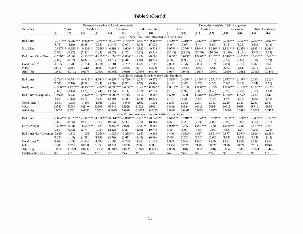
53

Table 9 (Cont’d)

Variables

Dependent variable: CAR of downgrades Dependent variable: CAR of upgrades

Crisis Credit Crisis Recession High Uncertainty Crisis Credit Crisis Recession High Uncertainty

(1) (2) (3) (4) (5) (6) (7) (8) (9) (10) (11) (12) (13) (14) (15) (16)

Panel D: Small size firms interacted with bad times

Bad times -0.781*** -0.782*** -0.882*** -0.979*** -0.946*** -0.746*** -0.469*** -0.483*** 0.430*** 0.318*** 0.513*** 0.440*** 0.746*** 0.355*** 0.200*** 0.191***

(8.75) (8.10) (9.28) (9.58) (10.42) (7.07) (8.07) (7.93) (4.97) (2.97) (5.44) (3.64) (8.15) (3.23) (3.89) (3.48)

SmallSize -0.897*** -0.656*** -0.826*** -0.538*** -0.893*** -0.609*** -0.932*** -0.711*** 1.978*** 1.376*** 1.944*** 1.316*** 1.891*** 1.245*** 1.865*** 1.266***

(8.95) (5.27) (7.91) (4.14) (8.67) (4.75) (8.55) (5.31) (17.45) (10.35) (17.40) (10.00) (21.49) (11.34) (13.71) (7.89)

Bad times×SmallSize -0.790** -0.367 -1.551*** -1.215*** -1.353*** -1.086** -0.294 -0.068 0.685** 0.673** 1.066*** 1.167*** 1.916*** 2.203*** 0.665*** 0.660***

(2.02) (0.82) (4.02) (2.87) (3.31) (2.41) (1.18) (0.23) (2.34) (1.98) (3.39) (3.19) (2.97) (2.83) (3.08) (2.59)

Good times Ŷ -1.705 -1.780 -1.714 -1.778 -1.681 -1.782 -1.635 -1.708 2.063 2.176 2.063 2.169 2.028 2.173 2.047 2.154

#Obs 70312 58885 70312 58885 70312 58885 68610 57550 66865 56433 66865 56433 66865 56433 64972 54943

Adj R-Sq 0.0059 0.0193 0.0073 0.0209 0.0075 0.0198 0.0046 0.0189 0.0170 0.0441 0.0176 0.0449 0.0202 0.0461 0.0165 0.0440

Panel E: No options firms interacted with bad times

Bad times -0.734*** -0.754*** -0.915*** -1.044*** -0.897*** -0.790*** -0.290*** -0.375*** 0.395*** 0.406*** 0.498*** 0.571*** 0.677*** 0.498*** 0.030 0.111*

(7.57) (7.10) (8.83) (9.44) (9.00) (6.90) (4.52) (5.46) (4.12) (3.45) (4.74) (4.30) (6.66) (4.13) (0.54) (1.81)

NoOptions -0.386*** 0.420*** -0.366*** 0.476*** -0.396*** 0.435*** -0.369*** 0.367** 1.091*** -0.160 1.050*** -0.229 1.006*** -0.309** 1.022*** -0.228

(3.63) (3.15) (3.29) (3.44) (3.55) (3.11) (3.22) (2.53) (8.15) (0.97) (8.05) (1.43) (9.96) (2.49) (6.61) (1.18)

Bad times×NoOptions -0.944* -0.742 -2.028*** -2.120*** -0.987** -0.716 -0.414 -0.108 0.609* 0.508 1.516*** 1.699*** 1.738** 1.994* 0.410 0.442

(1.82) (1.15) (3.72) (3.28) (2.20) (1.41) (1.44) (0.32) (1.70) (1.21) (3.56) (3.36) (1.96) (1.75) (1.60) (1.44)

Good times Ŷ -1.861 -1.957 -1.860 -1.945 -1.836 -1.949 -1.862 -1.931

2.245 2.363 2.241 2.353 2.210 2.353 2.297 2.387

#Obs 63540 52969 63540 52969 63540 52969 61821 51621 60619 50964 60619 50964 60619 50964 58710 49458

Adj R-Sq 0.0027 0.0201 0.0041 0.0221 0.0035 0.0202 0.0012 0.0193 0.0046 0.0465 0.0054 0.0476 0.0068 0.0480 0.0039 0.0457

Panel F: Low coverage firms interacted with bad times

Bad times -0.894*** -0.926*** -1.047*** -1.176*** -0.961*** -0.848*** -0.478*** -0.547*** 0.645*** 0.718*** 0.764*** 0.909*** 0.823*** 0.708*** 0.245*** 0.357***

(8.86) (8.36) (9.61) (9.96) (9.34) (7.33) (7.55) (8.16) (6.65) (6.28) (7.24) (7.05) (8.02) (6.09) (4.36) (5.97)

LowCoverage -0.579*** -0.081 -0.581*** -0.031 -0.452** 0.070 -0.483** -0.208 1.089*** 0.235 1.077*** 0.230 1.058*** 0.296 0.879*** 0.063

(2.69) (0.32) (2.74) (0.12) (2.12) (0.27) (1.99) (0.74) (5.84) (1.00) (5.84) (0.99) (5.83) (1.27) (4.20) (0.24)

Bad times×LowCoverage -0.925 -1.310 -1.195 -2.050** -1.929** -2.285*** -0.687 -0.366 0.446 1.282** 0.637 1.531*** 0.877 1.074* 0.826** 1.138**

(1.23) (1.45) (1.38) (1.98) (2.56) (2.61) (1.43) (0.60) (0.89) (2.26) (1.20) (2.64) (1.52) (1.84) (2.15) (2.45)

Good times Ŷ -1.621 -1.697 -1.626 -1.694 -1.609 -1.704 -1.563 -1.622

1.903 1.984 1.902 1.979 1.884 1.989 1.899 1.952

#Obs 61280 51950 61280 51950 61280 51950 59869 50831 59384 50527 59384 50527 59384 50527 57814 49264

Adj R-Sq 0.0032 0.0220 0.0037 0.0232 0.0042 0.0220 0.0020 0.0213 0.0034 0.0460 0.0038 0.0469 0.0045 0.0456 0.0024 0.0446

Controls, Ind. F.E. No Yes No Yes No Yes No Yes No Yes No Yes No Yes No Yes

54

Table 10: Analyst attrition in bad times Probits of analyst attrition are estimated for the recommendations sample (1993-2014). In the recommendations sample, variables

are averaged within each analyst-year combination and Disappear equals one when the analyst makes no recommendation in

I/B/E/S in the next year. The bad times indicator=1 if any month in the next year contains the relevant bad times period. Crisis is

defined as the periods Sep-Nov 1987 (1987 crisis), Aug-Dec 1998 (LTCM), or Jul 2007-Mar 2009 (Credit Crisis). Recession

represents NBER recessions, namely: Jul 1990-Mar 1991, Mar 2001-Nov 2001, and Dec 2007-Jun 2009. High Uncertainty

represents the highest tercile (over the period 1983-2014) of the Baker et al. (2016) uncertainty index. Rec Influ Prob is the

fraction of influential recommendation changes made by the analyst that year. Other control variables are as defined in relevant

earlier tables. In parentheses are z-statistics where *, **, and *** denote statistical significance (standard errors clustered by

analyst) at 10%, 5%, and 1% respectively.

Variables Dependent variable: Recommendations sample, Disappear from I/B/E/S next year

(1) (2) (3) (4) (5) (6) (7) (8)

Crisis 0.008* 0.010**

(1.81) (2.18)

Credit Crisis 0.034*** 0.037***

(6.11) (6.38)

Recession 0.042*** 0.034***

(8.67) (6.78)

High Uncertainty 0.026*** 0.028***

(5.20) (5.65)

Rec Influ Prob -0.030*** -0.020** -0.030*** -0.020** -0.032*** -0.023*** 0.009 0.019

(3.34) (2.18) (3.52) (2.27) (3.61) (2.62) (0.47) (1.05)

Crisis×Rec Influ Prob -0.034** -0.034**

(2.01) (1.97)

Credit Crisis×Rec Influ Prob -0.055*** -0.056***

(2.93) (2.91)

Recession×Rec Influ Prob -0.037** -0.029

(2.14) (1.62)

High Uncertainty×Rec Influ Prob -0.058*** -0.058***

(2.88) (2.90)

LFR -0.000 -0.000 -0.001 -0.000

(0.67) (0.73) (0.92) (0.75)

Relative Experience -0.000** -0.000** -0.000** -0.000**

(2.14) (2.27) (2.24) (2.43)

Log Broker Size -0.012*** -0.012*** -0.013*** -0.012***

(6.80) (6.78) (7.09) (6.95)

Log Size -0.003** -0.003** -0.004*** -0.004***

(2.40) (2.56) (2.97) (3.03)

Log BM -0.008*** -0.007** -0.006** -0.009***

(2.71) (2.35) (2.13) (3.25)

Momentum -0.024*** -0.023*** -0.025*** -0.024***

(5.58) (5.40) (5.93) (5.66)

Stock Volatility 0.895*** 0.973*** 0.782*** 0.819***

(7.65) (8.20) (6.83) (7.14)

Predicted Prob. 0.128 0.114 0.128 0.114 0.127 0.114 0.128 0.114

#Obs 38546 35508 38546 35508 38546 35508 38546 35508

55

Table 11: Panel regression of analyst activity in bad times The panel regressions estimate the effect of bad times on analyst forecast activity (1+an analyst’s # of forecasts per firm-quarter)

controlling for forecast, analyst, and firm characteristics. We define the starting and ending quarter of coverage using the first and

last one-quarter-ahead forecast of the analyst-firm-broker combination. We then count the number of quarterly earnings forecasts

per quarter for each calendar quarter. Bad times definitions are as follows: Crisis: Sep-Nov 1987 (1987 crisis), Aug-Dec 1998

(LTCM), or Jul 2007-Mar 2009 (Credit Crisis). Recession represents NBER recessions, namely: Jul 1990-Mar 1991, Mar 2001-

Nov 2001, and Dec 2007-Jun 2009. High Uncertainty represents the highest tercile (over the period 1983-2014) of the Baker et al.

(2016) uncertainty index. Analyst and forecast characteristics are the averages within the analyst-firm quarter. Optimistic

Forecast is an indicator variable equal to one if the forecast is above the final consensus, LFR is the analyst’s prior-year leader-

follower ratio (computed from forecasts), Star Analyst is from the Institutional Investor poll, Relative Experience is the

difference between the analyst’s experience (in quarters) against the average of peers covering the same firm, Accuracy Quintile

is the average forecast accuracy quintile of the analyst’s past-year’s covered firms (quintile 5=most accurate), Days to Annc is the

number of days from the forecast to the earnings announcement date, Multiple Forecast Day is a dummy indicating that more

than one analyst issued a forecast on that day, Broker Size is the number of analysts employed, # Analysts is 1+ the number of

analysts covering the firm, Size is last June’s market cap, BM is the book-to-market ratio, Momentum is the month t-12 to t-2 buy-

and-hold return, and Dispersion is the dispersion of forecasts making up the final consensus. In parentheses are t-statistics based

on standard errors clustered by industry-quarter, where *, **, and *** denote statistical significance at 10%, 5%, and 1%

respectively. Industry fixed effects (F.E.) rely on the Fama-French 30-industry groupings.

Variables Dependent variable: Log (1 + # forecasts per firm-quarter)

(1) (2) (3) (4) (5) (6) (7) (8) Crisis 0.063*** 0.067*** (6.34) (10.27) Credit Crisis 0.094*** 0.082***

(8.11) (10.75) Recession 0.069*** 0.069*** (8.21) (11.74) High Uncertainty 0.048*** 0.030***

(7.92) (7.16) Optimistic Forecast 0.011*** 0.011*** 0.011*** 0.011*** (8.82) (8.78) (8.91) (8.74) LFR 0.002*** 0.002*** 0.002*** 0.003*** (11.27) (11.01) (11.11) (12.41) Star Analyst -0.028*** -0.027*** -0.029*** -0.028*** (13.72) (13.47) (13.98) (13.25) Relative Experience 0.000*** 0.000*** 0.000*** 0.000*** (5.08) (5.01) (5.15) (5.78) Accuracy Quintile 0.028*** 0.028*** 0.029*** 0.028*** (25.97) (25.95) (26.23) (25.69) Log Days to Annc -0.019*** -0.020*** -0.019*** -0.020*** (9.45) (9.63) (9.12) (9.70) Mutiple Forecast Day -0.038*** -0.038*** -0.038*** -0.038*** (21.02) (21.35) (21.25) (20.30) Log Broker Size 0.037*** 0.037*** 0.037*** 0.037*** (39.39) (39.31) (39.23) (38.39) Log # Analysts 0.261*** 0.260*** 0.259*** 0.258*** (61.69) (61.77) (62.16) (58.63) Log Size -0.039*** -0.038*** -0.038*** -0.039*** (32.33) (32.31) (32.44) (31.81) Log BM 0.008*** 0.008*** 0.009*** 0.005*** (5.45) (5.23) (6.68) (3.15) Momentum -0.004* -0.003 -0.001 -0.007***

(1.81) (1.57) (0.53) (3.08) Dispersion 0.018*** 0.018*** 0.017*** 0.019*** (12.72) (12.72) (12.75) (12.49) Intercept 0.642*** 0.497*** 0.641*** 0.500*** 0.639*** 0.492*** 0.619*** 0.501***

(194.02) (28.80) (198.10) (29.08) (189.89) (28.46) (157.11) (28.86)

Good times Ŷ 0.642 0.680 0.641 0.680 0.639 0.678 0.619 0.667 Observations 1916213 1250891 1916213 1250891 1916213 1250891 1850104 1201285 Adj R-Sq 0.0021 0.1001 0.0037 0.1006 0.0031 0.1007 0.0035 0.0981 Industry F.E. No Yes No Yes No Yes No Yes

56

Table 12: Analyst report length in bad times The list of all U.S. analyst reports issued by one large U.S. broker from 1994-2014 is downloaded from Thomson ONE (up to

Sep 2011) and Thomson Eikon (from Oct 2011 onwards) and the number of pages in each report is regressed against a bad times

dummy and control variables. Bad times definitions are as follows: Crisis: Sep-Nov 1987 (1987 crisis), Aug-Dec 1998 (LTCM),

or Jul 2007-Mar 2009 (Credit Crisis). Recession represents NBER recessions, namely: Jul 1990-Mar 1991, Mar 2001-Nov 2001,

and Dec 2007-Jun 2009. High Uncertainty represents the highest tercile (over the period 1983-2014) of the Baker et al. (2016)

uncertainty index. Beta is the stock’s market beta based on three years of past monthly returns. Size Quintile is based on the

stock’s prior June’s market cap using NYSE breakpoints. Momentum Quintile is based on the month t-12 to t-2 buy-and-hold

stock return sorted as at month t-1. BM Quintile is based on the firm’s book-to-market ratio. Stock Volatility is the month t-1

volatility of daily stock returns. Earnings Annc Dummy (Guidance Dummy) indicates that the analyst report is issued within three

trading days of an earnings announcement (earnings guidance). Earnings announcement dates are from Compustat and guidance

dates are from First Call Guidelines and I/B/E/S Guidance. In parentheses are t-statistics based on standard errors clustered by the

date of the analyst report, where *, **, and *** denote statistical significance at 10%, 5%, and 1% respectively. Industry fixed

effects (F.E.) rely on the Fama-French 30-industry groupings.

Variables Dependent variable: Number of pages in an analyst report

(1) (2) (3) (4) (5) (6) (7) (8)

Crisis 1.336*** 1.552***

(8.84) (9.99)

Credit Crisis 1.916*** 1.991***

(13.21) (12.34)

Recession -0.928*** -0.098

(5.80) (0.62)

High Uncertainty 1.429*** 1.356***

(13.61) (14.35)

Beta 0.386*** 0.379*** 0.389*** 0.396***

(10.41) (10.24) (10.37) (10.35)

Size Quintile 0.091*** 0.094*** 0.086*** 0.100***

(3.68) (3.79) (3.43) (3.94)

Momentum Quintile -0.172*** -0.171*** -0.150*** -0.152***

(7.92) (7.89) (6.81) (6.86)

BM Quintile 0.072*** 0.071*** 0.077*** 0.093***

(3.14) (3.08) (3.34) (3.94)

Stock Volatility -68.509*** -68.194*** -66.087*** -66.818***

(26.86) (26.96) (24.67) (26.31)

Earnings Annc Dummy -0.068 -0.101 -0.023 0.026

(0.77) (1.13) (0.26) (0.29)

Guidance Dummy 0.644*** 0.636*** 0.644*** 0.501***

(8.97) (8.89) (8.87) (6.93)

Intercept 10.237*** 11.305*** 10.215*** 11.296*** 10.433*** 11.292*** 9.678*** 10.626***

(178.98) (66.07) (179.86) (66.18) (182.87) (65.83) (122.69) (58.01)

Good times Ŷ 10.237 10.220 10.215 10.208 10.433 10.345 9.678 9.706

#Obs 85525 84707 85525 84707 85525 84707 81583 80806

Adj R-Sq 0.0024 0.0552 0.0043 0.0566 0.0015 0.0520 0.0097 0.0624

Industry F.E. No Yes No Yes No Yes No Yes

57

Table 13: Response of peer firms to recommendation changes in bad times The panel regressions estimate the effect of recommendation changes on peer firms’ two-day CARs (in percent) during bad times, controlling for recommendation, firm, and analyst

characteristics. Peer firms are firms in the same industry which did not experience a recommendation by the same analyst that day but for which the analyst has issued a recommendation on in

the last one year. The CAR benchmark is a characteristics-matched DGTW portfolio for the peer firm. The sample is from 1993-2014. Recommendation changes are the current rating minus

the individual analyst’s prior outstanding rating (initiations and reiterations are excluded). Recommendation changes made around earnings announcement and guidance days, and on multiple-

recommendation days are excluded following Loh and Stulz (2011). Bad times definitions are as follows: Crisis: Sep-Nov 1987 (1987 crisis), Aug-Dec 1998 (LTCM), or Jul 2007-Mar 2009

(Credit Crisis). Recession represents NBER recessions, namely: Jul 1990-Mar 1991, Mar 2001-Nov 2001, and Dec 2007-Jun 2009. High Uncertainty represents the highest tercile (over the

period 1983-2014) of the Baker et al. (2016) uncertainty index. Control variables are as defined in Table 3. In parentheses are t-statistics based on standard errors clustered by calendar day,

where *, **, and *** denote statistical significance at 10%, 5%, and 1% respectively. Industry fixed effects (F.E) rely on the Fama-French 30-industry groupings.

Variables Dependent variable: CAR of peer firms of downgrades Dependent variable: CAR of peer firms of upgrades

(1) (2) (3) (4) (5) (6) (7) (8) (9) (10) (11) (12) (13) (14) (15) (16) Crisis -0.104* -0.105* -0.021 -0.042 (1.78) (1.71) (0.36) (0.73)

Credit Crisis -0.131** -0.153** -0.046 -0.077 (2.09) (2.32) (0.67) (1.20) Recession -0.163** -0.196** 0.020 -0.052 (2.44) (2.54) (0.31) (0.84) High Uncertainty -0.035 -0.019 -0.034 -0.028 (0.96) (0.47) (1.10) (0.92) LFR 0.001 0.001 0.001 0.000 0.007* 0.007* 0.007* 0.006 (0.19) (0.19) (0.21) (0.07) (1.69) (1.69) (1.70) (1.57) Star Analyst -0.040 -0.040 -0.040 -0.040 0.079** 0.078** 0.079** 0.076**

(0.86) (0.86) (0.87) (0.84) (2.09) (2.09) (2.10) (1.97) Relative Experience -0.001 -0.001 -0.001 -0.001 -0.000 -0.000 -0.000 0.000 (0.78) (0.76) (0.72) (1.08) (0.08) (0.07) (0.08) (0.15) Accuracy Quintile 0.005 0.005 0.005 0.001 -0.014 -0.013 -0.014 -0.014 (0.13) (0.13) (0.12) (0.02) (0.38) (0.36) (0.38) (0.39) Log Broker Size -0.041*** -0.042*** -0.040** -0.041** 0.024* 0.024* 0.025* 0.029** (2.61) (2.69) (2.56) (2.56) (1.80) (1.74) (1.83) (2.08) Log # Analysts -0.040 -0.042 -0.042 -0.030 0.063** 0.062** 0.064** 0.065** (1.46) (1.52) (1.53) (1.10) (2.50) (2.42) (2.51) (2.53) Log Size 0.000 0.002 0.005 -0.004 -0.000 0.001 0.000 -0.002 (0.04) (0.19) (0.41) (0.37) (0.04) (0.08) (0.02) (0.19) Log BM -0.006 -0.005 -0.006 -0.009 0.017 0.017 0.017 0.017 (0.34) (0.28) (0.35) (0.48) (1.04) (1.06) (1.05) (1.05) Momentum -0.040* -0.041* -0.049** -0.036* -0.042** -0.043** -0.044** -0.041** (1.84) (1.88) (2.25) (1.68) (2.10) (2.14) (2.18) (2.01) Stock Volatility -1.190 -1.124 -0.590 -1.634 3.681*** 3.761*** 3.808*** 3.488*** (1.02) (0.96) (0.47) (1.41) (3.53) (3.61) (3.68) (3.18) Intercept -0.054*** 0.185 -0.053*** 0.169 -0.045*** 0.122 -0.059*** 0.247 0.110*** -0.171 0.112*** -0.183 0.105*** -0.185 0.122*** -0.155 (3.37) (0.91) (3.34) (0.84) (3.04) (0.60) (3.68) (1.19) (8.74) (1.08) (8.92) (1.15) (8.50) (1.17) (8.20) (0.96)

Good times Ŷ -0.054 -0.066 -0.053 -0.063 -0.045 -0.053 -0.059 -0.077 0.110 0.120 0.112 0.123 0.105 0.121 0.122 0.127 #Obs 68725 58670 68725 58670 68725 58670 67111 57357 65482 56238 65482 56238 65482 56238 63670 54765 Adj R-Sq 0.0002 0.0017 0.0002 0.0019 0.0005 0.0022 0.0000 0.0017 -0.0000 0.0020 0.0000 0.0021 -0.0000 0.0020 0.0000 0.0020 Industry F.E. No Yes No Yes No Yes No Yes No Yes No Yes No Yes No Yes

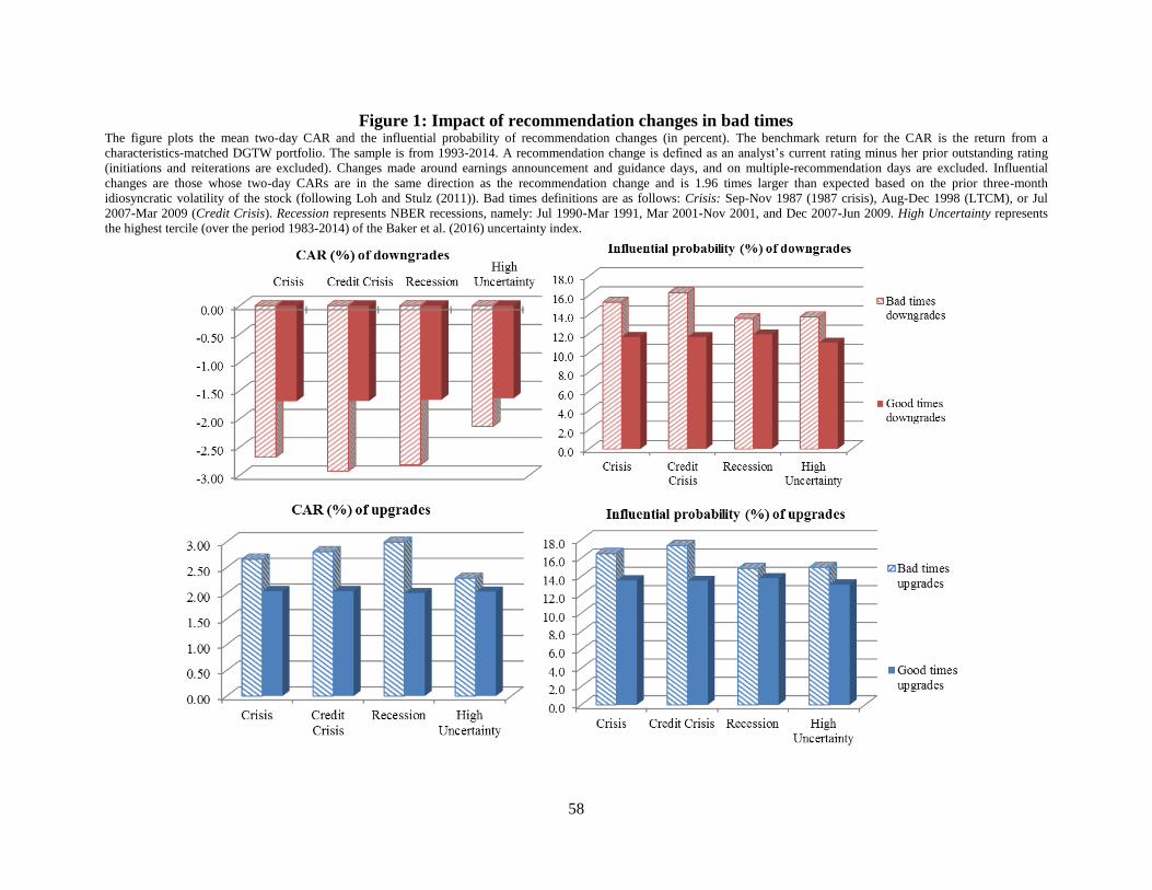
58

Figure 1: Impact of recommendation changes in bad times The figure plots the mean two-day CAR and the influential probability of recommendation changes (in percent). The benchmark return for the CAR is the return from a

characteristics-matched DGTW portfolio. The sample is from 1993-2014. A recommendation change is defined as an analyst’s current rating minus her prior outstanding rating

(initiations and reiterations are excluded). Changes made around earnings announcement and guidance days, and on multiple-recommendation days are excluded. Influential

changes are those whose two-day CARs are in the same direction as the recommendation change and is 1.96 times larger than expected based on the prior three-month

idiosyncratic volatility of the stock (following Loh and Stulz (2011)). Bad times definitions are as follows: Crisis: Sep-Nov 1987 (1987 crisis), Aug-Dec 1998 (LTCM), or Jul

2007-Mar 2009 (Credit Crisis). Recession represents NBER recessions, namely: Jul 1990-Mar 1991, Mar 2001-Nov 2001, and Dec 2007-Jun 2009. High Uncertainty represents

the highest tercile (over the period 1983-2014) of the Baker et al. (2016) uncertainty index.

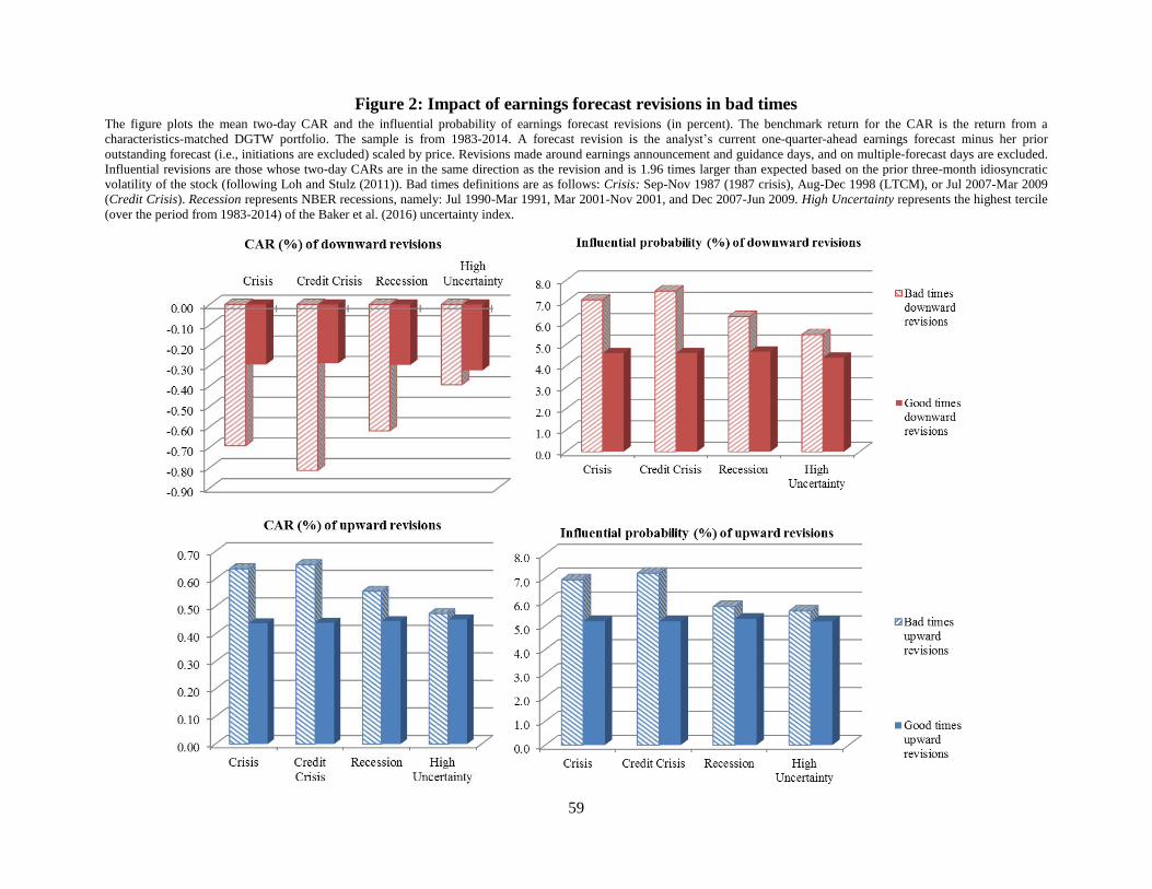
59

Figure 2: Impact of earnings forecast revisions in bad times The figure plots the mean two-day CAR and the influential probability of earnings forecast revisions (in percent). The benchmark return for the CAR is the return from a

characteristics-matched DGTW portfolio. The sample is from 1983-2014. A forecast revision is the analyst’s current one-quarter-ahead earnings forecast minus her prior

outstanding forecast (i.e., initiations are excluded) scaled by price. Revisions made around earnings announcement and guidance days, and on multiple-forecast days are excluded.

Influential revisions are those whose two-day CARs are in the same direction as the revision and is 1.96 times larger than expected based on the prior three-month idiosyncratic

volatility of the stock (following Loh and Stulz (2011)). Bad times definitions are as follows: Crisis: Sep-Nov 1987 (1987 crisis), Aug-Dec 1998 (LTCM), or Jul 2007-Mar 2009

(Credit Crisis). Recession represents NBER recessions, namely: Jul 1990-Mar 1991, Mar 2001-Nov 2001, and Dec 2007-Jun 2009. High Uncertainty represents the highest tercile

(over the period from 1983-2014) of the Baker et al. (2016) uncertainty index.