is subject to Institution of Electrical and Electronic

This paper is a post-print of a paper submitted to and accepted for publication in IEEE Journal of Emerging and Selected Topics in Power Electronics and

is subject to Institution of Electrical and Electronic Engineering Copyright. The copy of record is available at IEEE Xplore Digital Library.

1

Abstract- This paper develops a small-signal impedance model

of modular multilevel converters (MMCs) using harmonic state-

space (HSS) method and studies the stability in a multiple

converter scenario. In order to simplify analysis on the coupling

characteristics between different frequencies in MMCs, the

proposed model is developed in the positive-negative-zero (PN0)

sequence-frame, where the zero-sequence current in three-phase

three-wire system is directly set to zero without introducing

complicated method. A simple 2 by 2 admittance matrix in PN0-

frame is extracted from the MMC small-signal model for ease of

system stability analysis. Using the developed impedance model,

the multi-infeed interaction factor (MIIF) measure is adopted to

analyze the most significant interactions for multi-infeed

converter systems to be prioritized. Different outer-loop

controllers are adopted and compared in the analysis to illustrate

the effect of different control modes on converter impedance and

system stability. Analytical studies and time-domain simulation

results are provided to validate the proposed model and stability

analysis.

Index Terms- Admittance, harmonic state-space (HSS), modular

multilevel converter (MMC), stability.

I. INTRODUCTION

With rapidly increased penetration of renewable energy and

distributed generation, and the increased use of HVDC systems

for interconnection and renewable integration, system stability

of grid-connected converters becomes a significant challenge

[1]. Hence, effective methods to identify the source of resonance and to mitigate the stability problems becomes

critically important. To assess the system stability and dynamic

interactions between grid and converters, the impedance-based

stability analysis [2][3] is an effective method of identifying

potential frequencies of disturbance to which an individual

converter may be vulnerable to destabilizing behavior.

Therefore, an accurate impedance modelling of converters is

required. Modular multilevel converter (MMC) is now being

widely used for HVDC systems [4-6]. However, due to its

inherently complex behavior such as internal circulating current

and submodule (SM) capacitor voltage ripple, accurately

modelling the impedance or admittance of MMC is a challenging task [7][8]. The consequences of not modelling

This work is supported in part by the UK National HVDC Center. Y. Chen, L. Xu, and A. Egea are with the Department of Electronic

and Electrical Engineering, University of Strathclyde, Glasgow G1 1XW, U.K. (e-mail: [email protected], [email protected], [email protected] ). B. Marshall, Md Rahman, O. D. Adeuyi are with the UK National HVDC Centre, Cumbernauld, G68 0FQ, UK. (email: [email protected], [email protected], [email protected] )

these aspects could lead to a displacement or deletion of

frequencies of interaction and a mis-estimation of the

magnitude of the impedance changes at those points. Various studies have been carried out on developing MMC

impedance models. In [9], an analytical sequence impedance

model of a three-phase MMC is derived with the internal MMC

dynamics, following the same approach used for 2-level VSCs.

However, the 2nd harmonic in the arm current and PLL are not

considered in the model. In [10], the AC side input admittances

of the MMC under various control strategies are derived,

though the circulating current controller is not included. Reference [11] focuses on the impact of different current-

control schemes on the shape of MMC admittance, considering

the 2nd internal harmonic current. However, a large resistive

load is added at the AC side to provide increased passive

damping, so that high-order harmonics are not presented in the

system and not considered in [11]. However, in real systems,

such strong passive damping does not exist and harmonic or

inter-harmonic resonances are a major concern and must be

modelled.

The Harmonic State-Space (HSS) method proposed to analyze linear time-periodic (LTP) system [12], models not

only the steady-state harmonics in LTP systems, but also the

dynamics of the harmonics during transients. Consequently,

HSS method has been widely used to model power networks

and converters, e.g., static synchronous compensators [13],

LCC converters [12], transmission lines [14], and two-level

VSCs [15]. Recently, HSS method has been used to model

MMC impedance considering the impact of the internal

harmonics [16]-[18]. Since the Fourier coefficients matrices in

the HSS model are diagonal-constant matrices (Toeplitz

matrices) [16], the MMC small-signal model based on HSS can

be easily extended to any harmonic order. Hence, the dynamics of high-order harmonics in MMC can be fully considered.

However, various problems and limitations still exist in the

proposed HSS-based MMC small-signal modelling methods

[16]-[18]. In [16], a single-phase MMC model is developed and

the impedance that reflects the voltage and current at the same

frequency is derived but the couplings at different frequencies

generated by the internal harmonics of MMC, are not taken into

account. Impedance models of three-phase four-wire MMC

systems, in which both the MMC DC mid-point and the AC

neutral point are grounded providing a circulation path for the

zero-sequence current, are derived in [17][18]. However, in reality, MMC systems are likely to be configured as an

equivalent three-phase three-wire system without the low

impedance path for the zero-sequence current. To describe the

MMC zero-sequence current on the MMC AC side in three-

phase three-wire systems, zero-sequence voltage compensation

is proposed to add into the single-phase model in [17] and the

MMC Impedance Modelling and Interaction

of Converters in Close Proximity Yin Chen, Lie Xu, Senior Member, IEEE, Agustí Egea-Àlvarez, Member, IEEE, Benjamin

Marshall, Md Rahman, and Oluwole D. Adeuyi

mailto:[email protected]








2

single-phase impedance is obtained for three-phase system

stability assessment. The MMC controllers in the models also

adopt the proportional resonant (PR) controller in the abc-

frame, implying that the controls for phase a, b, and c are totally

independent and identical. However, for MMC controller implemented in αβ-frame or dq-frame, the single-phase

modelling method is inadequate and is thus unsuitable for three-

phase MMC system.

In the latest study on MMC impedance modelling, reference

[19] provides a comprehensive three-phase HSS model of

MMC. Similar to [17], the DC mid-point voltage is

compensated using the AC neutral point voltage to eliminate

the zero-sequence current. However, when developing the

small-signal model, the expression of the neutral point voltage

involves the steady-state value and the perturbation variables of

three-phase voltages as well as the control signal of the arms,

which lead to an extra complex calculation in the HSS model. In [19], the complex vector representation of the controllers in

dq-frame obtained based on the transfer function, has to be

transformed to the αβ-frame before being integrated into the

MMC model to obtain the impedance in the positive-negative-

zero (PN0) sequence frame, thus leading to complicated

transformation and calculation.

In addition, the MMC impedance obtained in [19] is a 10 by

10 matrix. In order to simplify the process of stability

assessment, a single input and single output (SISO) equivalent

impedance of the MMC is derived by considering the grid side

impedance. However, if the grid structure is more complex, e.g., there are other converters connected to the grid in close

proximity, the grid impedance seen by the MMC will also

become complicated. Thus it is difficult to simplify the 10 by

10 matrix of MMC impedance to a SISO equivalent. Therefore,

a MMC impedance independent of the grid side impedance and

in simple form is more beneficial for system stability

assessment with multiple converters. MMC represented by 2 by

2 impedance matrix in modified sequence-domain [20] is

developed in [21][22]. However, in the modified sequence-

domain the frequencies of the coupling admittance cannot be

represented. Moreover, unlike the impedance in the sequence

domain, the MMC impedance in the modified sequence domain cannot be measured directly in time domain due to the existence

of frequency shift between the modified sequence domain and

sequence domain. In [23], a MMC 2 by 2 impedance matrix is

derived to capture the characteristics of frequency coupling in

sequence frame. However, the work focuses on the coupling

between the AC system and DC system of the MMC and the

dynamic of the PLL in AC side is not considered.

Considering the limitations in the existing modelling

approach and limited work on assessing system stability with

multiple MMCs, the main contributions of this paper are:

• Addressing the non-existence zero sequence current in three-phase three-wire systems, instead of adding a

compensation voltage [17][19], the zero-sequence current is

directly forced to zero thus providing a simplified modelling

approach;

• When mapping the dq-controllers, their transfer functions

are directly transformed from dq to the PN0-frame which

significantly simplifies the modelling process compared to

[19];

• Simplification of the high-dimensional MMC admittance to

a 2 by 2 matrix based on the characteristics of MMC

harmonics in PN0-frame. The MMC impedance

independent of the grid side impedance with simpler form

can be more suitable for system stability assessment

especially when multiple converters are considered;

• Interaction of converters in close proximity is studied using

the developed models and system stability assessment in

case of multiple MMCs in a network are carried out

considering the multi-infeed interaction factor (MIIF).

The rest of the paper is organized as follows. Section Ⅱ

presents the HSS modelling procedure of three-phase MMC. In

Section Ⅲ, the small-signal admittance of MMC in PN0-frame

is derived while Section Ⅳ verifies the proposed model and

conducts the stability assessment. Section Ⅴ analyzes the

stability of converters in close proximity and Section Ⅵ draws

the conclusions.

II. HSS MODELLING OF THREE-PHASE MMC

A. Linearizing MMC model in abc-frame

The equivalent circuit of the MMC average model [24][25]

is depicted in Fig. 1, where a lumped capacitor Cm and a voltage

source are used to mimic the dynamic of each arm. Take phase

a as an example, Va and Zg represent the grid voltage and

impedance seen at the MMC AC terminals, i.e., the impedance

of converter transformer is incorporated into Zg. Δvpa is a small

AC perturbation voltage.cuav and clav

are the sum of the

capacitor voltages of the SMs in the upper and lower arms,

respectively. The upper and lower arm current are iua and ila, the

arm voltage vua and vla, and modulation control signal nua and

nla. vga and iga are the voltage and current on the AC side of the

MMC, respectively. The DC voltage Vdc is assumed to be

constant. Since the system is in a three-phase three-wire

connection, the voltage of the DC mid-point is vn.

Zg

YMMC

vp

Grid

Va

Vb

Vc

Rm , Lm

ila ilb ilc

iua iub iuc

iga

igb

igc

𝑣𝑢𝑎 =

𝑛𝑢𝑎𝑣𝑐𝑢𝑎∑

+1

2𝑉𝑑𝑐

−1

2𝑉𝑑𝑐

vga

vgb

vgc

𝑣𝑐𝑢𝑎∑

nuaiua

𝑣𝑐𝑙𝑎∑

nlaila

+

-

+

-

Cm

Rm , Lm

Cm

Δvpa

Δvpb

Δvpc

vnZg

Zg

𝑣𝑙𝑎 =

𝑛𝑙𝑎𝑣𝑐𝑙𝑎∑

Fig. 1 Equivalent circuit of a three-phase MMC

For ease of analysis, the three-phase quantities are defined in

3 by 1 matrices as vgabc, igabc, cuabc

v , clabc

v , vuabc, iuabc, vlabc, ilabc,

icabc, Vdc, and vn, whereas nuabc and nlabc are 3 by 3 diagonal

matrices.

For a three-phase MMC, the relationship between the arm

voltage and the equivalent capacitor voltage of the SMs can be

expressed as:

= , =uabc uabc cuabc labc labc clabc

v n v v n v (1)

The internal dynamics between equivalent capacitor voltage

of SMs and the arm current are depicted as:



3

= , =cuabc clabcm uabc uabc m labc labc

d dC C

dt dt

v v

n i n i (2)

The arm voltages vuabc and vlabc, and the capacitor voltages

cuabc

v and clabc

v all contains multiple harmonics [24]. It

indicates that MMC has multi-frequency responses due to its

significant steady-state harmonic components in the arm

currents and capacitor voltages.

The common-mode current that circulates inside the arms

and the AC side current are denoted as:

( )= + 2cabc uabc labci i i (3)

gabc uabc labc= −i i i (4)

The voltage on the AC terminal of MMC and the currents

and voltages of the arms have the following relationship:

+2

2

uabc dcgabc m m uabc uabc n

labc dcgabc m m labc labc n

dL R

dt

dL R

dt

+ + = +

− − − = − +

i Vv i v v

i Vv i v v

(5)

where vn=[vn, vn, vn]T and the DC mid-point voltage vn is

obtained as [17]

6

ua cua la cla ub cub la clb uc cuc lc clcn

n v n v n v n v n v n vv

− + − + −= (6)

Combining (1)-(4) with (5) and considering small

perturbations, the MMC small-signal state-space model in abc-

frame can be expressed as:

=-2 2 2

2

=-

2 2+

cabc m uabc labc cuabccabc cuabc clabc uabc

m m m m

clabclabc

m

gabc m uabc labc cuabcgabc cuabc clabc uabc

m m m m

clabclabc pabc n

m m m

cuabc

d R

dt L L L L

L

d R

dt L L L L

L L L

d

− − −

−

− + −

− +

i N N Vi v v n

Vn

i N N Vi v v n

Vn v v

v= +

2 2

= +2 2

gabcuabc uabc cabccabc gabc uabc uabc

m m m m

gabcclabc labc labc cabccabc gabc labc labc

m m m m

dt C C C C

d

dt C C C C

+ + − −

IN N Ii i n n

Iv N N Ii i n n

(7)

where variables in capital form denote the values at the steady-

state operation point and variables with Δ denote the small

perturbations. The matrix Δvn is equal to [Δvn, Δvn, Δvn]T and the

component Δvn can be derived by linearizing (6) as:

6

6

6

ua cua la cla ua cua la clan

ub cub la clb ub cub la clb

uc cuc lc clc uc cuc lc clc

N v N v n V n Vv

N v N v n V n V

N v N v n V n V

− + −=

− + −+

− + −+

(8)

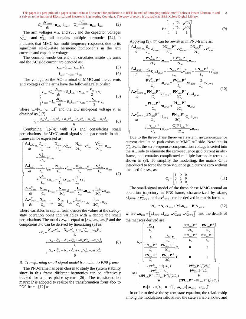
B. Transforming small-signal model from abc- to PN0-frame

The PN0-frame has been chosen to study the system stability

since in this frame different harmonics can be effectively

tracked for a three-phase system [26]. The transformation matrix P is adopted to realize the transformation from abc- to

PN0-frame [12] as:

2 43 3

4 23 3

1

= 11 1 1

P

j j

j j

e e

e e (9)

Applying (9), (7) can be rewritten in PN0-frame as: -1 -1

00 0 0

-1 -1

0 0

-1 -10

0 0 0

-1 -1

0

=-2 2

2 2

=-

+

cPN m uabc labccPN cuPN clPN

m m m

cuabc clabcuPN lPN

m m

gPN m uabc labcz gPN cuPN clPN

m m m

cuabc clabcuPN

m

d R

dt L L L

L L

d R

dt L L L

L

− −

− −

− +

−

i PN P PN Pi v v

PV P PV Pn n

i PN P PN PC i v v

PV P PV Pn 0 0

-1 -1

00 0

-1-1

0 0

-1 -1

00 0

1 -1-1

0 0

2

=2

+2

=2

+2

lPN pPN

m m

cuPN uabc uabccPN z gPN

m m

gabccabcuPN uPN

m m

clPN labc labccPN z gPN

m m

m gabccabclPN lPN

m m

L L

d

dt C C

C C

d

dt C C

C C

−

−

+

+

−

−

n v

v PN P PN Pi C i

PI PPI Pn n

v PN P PN Pi C i

C PI PPI Pn n

(10)

Due to the three-phase three-wire system, no zero-sequence

current circulation path exists at MMC AC side. Note that in

(7), Δvn is the zero-sequence compensation voltage inserted into

the AC side to eliminate the zero-sequence grid current in abc-

frame, and contains complicated multiple harmonic terms as

shown in (8). To simplify the modelling, the matrix Cz is

introduced to force the zero-sequence grid current zero without

the need for Δvn, as:

1 0 00 1 00 0 0

z

=

C (11)

The small-signal model of the three-phase MMC around an

operation trajectory in PN0-frame, characterized by ΔicPN0,

ΔigPN0, 0cuPN

v and

0clPN

v , can be derived in matrix form as

0 0 0 0=

PN s PN PN pPN+ +x A x M n B v (12)

where 0 0 0 0 0

T

PN cPN gPN cuPN clPN

= x i i v v and the details of

the matrices derived are: 1 1

1 1

1 1

1 1

- - -2 2

- -

=

2

-2

m uabc labc

m m m

m uabc labcz

m m m

s

uabc uabcz

m m

labc labcz

m m

R

L L L

R

L L L

C C

C C

− −

− −

− −

− −

PN P PN PI 0

PN P PN P0 C

APN P PN P

C 0 0

PN P PN PC 0 0

( )

( )

( )

( )

11

11

1 1

1 1

--

-=

(2 ) 2

(2 ) 2

clabc mcuabc m

cuabc mcuabc m

cabc gabc m

cabc gabc m

2L2L

LL

C

C

− −

− −

− −

− −

+

−

PV PPV P

PV PPV PM

0PI P PI P

PI P PI P0

0 0 0= -2 , =T T

m PN uPN lPNLB 0 I 0 0 n n n

In order to derive the system state equation, the relationship

among the modulation ratio ΔnPN0, the state variable ΔxPN0, and



4

the input variable ΔvpPN0 need be identified in PN0-frame.

When MMC controllers are considered, the variation of the

modulation ratio ΔnPN0 depends on the control variables of the

controllers. The control variables of the MMC generally include

the AC current and voltage, as well as the internal circulating current. Thus, the small signal upper and low arm modulation

ratios can be expressed as:

0 0 0 0 0 0 0

0 0 0 0 0 0 0

=-

=

uPN iPN gPN vPN gPN ccPN cPN

lPN iPN gPN vPN gPN ccPN cPN

− −

+ −

n G i G v G i

n G i G v G i (13)

where GiPN0, GvPN0 and GccPN0 are the gain matrices of the AC

current, AC voltage, and circulating current in the PN0-frame,

respectively.

Rewriting (13) in matrix form yields the relationship among

the modulation ratio ΔnPN0, the state variable ΔxPN0, and the

voltage ΔvpPN0 as:

0 0 0=PN A PN B pPN + n G x G v (14)

where 0 0

0 0

- -

-

ccPN iPN

A

ccPN iPN

=

G G 0 0G

G G 0 0 and 0

0

- vPN

B

vPN

=

GG

G.

Substituting (14) into (12) derives the small-signal state-

space equation of the three-phase MMC in PN0-frame as:

0 0 0=( ) ( )

PN s PN pPN+ + +A Bx A MG x B MG v (15)

C. MMC small-signal model based on HSS

All the state variables in (15) are periodic signals in steady-

state, and the MMC is essentially a time-periodic system, i.e.,

the matrices As, B, M, GA and GB are periodic [16]. Based on

the HSS modelling method [12], the MMC time-domain state-

space model (15) is transformed to the small-signal HSS model in frequency-domain to obtain a linear time-invariant (LTI)

system expressed as:

( )

0 0

0

=( [ ]+ [ ] )

[ ]+ [ ]

PN s A PN

B pPN

s −

+

X A M HG Q X

B M HG V (16)

where [ ]s A , [ ] B and [ ] M are Toeplitz matrices. HGA is

the control transfer matrix associated with the harmonic state

variables, HGB is the one with the harmonic input variables at

different frequencies, and their specific expressions are decided

by the controller. ΔXPN0 and ΔVpPN0 are the harmonic state

variable matrices and the input matrix in harmonic frequency,

respectively. The expressions of [ ]s A , [ ] B , [ ] M , HGA,

HGB, Q, ΔXPN0 and ΔVpPN0 are given in the Appendix.

To establish a complete small-signal MMC model, it is

necessary to include various controllers. In (16), HGA and HGB are the transfer function matrices determined by the controller

in PN0-frame. Therefore, to derive the small-signal impedance

of MMC, the transfer functions of specific controllers should be

established in the actual frame where they are implemented and

then transformed to PN0-frame. This enables different MMC

controllers, which are usually implemented in different frames,

e.g., PR circulating current controller in abc-frame and PI AC

current controller in dq-frame, to be accurate modelled in the

PN0-frame. The detailed procedures to determine the transfer

function matrices HGA and HGB in the small-signal model are

described in the following subsections.

D. Circulating current suppression controller (CCSC)

The circulating current predominantly contains a series of

even harmonics, in which the second-order harmonic dominates

[19]. The objective of CCSC is to suppress the circulating

current as Fig. 2 shows a typical implementation in in which 3

PR controller tuned at double fundamental frequency (2ω0) are

used, one for each phase.

s2+2ωcs +4ω02

+_

HPF

Krp

PR controller

+

+

Krr s

++0

2/Vdc

n2abc

icabc

Fig. 2 Diagram of circulating current suppression controller

The transfer function of the PR controller is [27]

2 2

0

( )2 4

rrPR rp

c

KG s K

s s = +

+ + (17)

where Krp and Krr are the proportional and resonant coefficients

of the PR controller, respectively. ωc is the cutoff frequency.

The high pass filter (HPF) filters out the DC component in

the common mode current, and its transfer function is:

2

2 2( )

2HPF

n n

sG s

s s =

+ + (18)

where ωn is the un-damped natural frequency and ζ is the

damping factor [30].

Thus, the double frequency output modulation signal by the

CCSC and the circulating current have the following

relationship:

2

2

2

( )

a ca

b ccabc cb

c cc

n i

n s i

n i

=

G (19)

where Gccabc(s) is the circulating current transfer function

matrix in abc-frame, and is given as: ( ) ( ) 0 0

2( ) 0 ( ) ( ) 0

0 0 ( ) ( )

HPF PR

ccabc HPF PR

dc

HPF PR

G s G s

s G s G sV

G s G s

−

=

G (20)

The corresponding CCSC transfer function in PN0-frame

GccPN0(s), as part of HGA in (16), can be derived as:

-1

0 (s)= (s)ccPN ccabc G P G P (21)

E. AC terminal current controller

The AC terminal current control loop is typically

implemented in dq-frame fixed to the voltage Vg at converter

AC connection point and its block diagram is presented in Fig. 3, together with the PLL. The output of the current control loop

is the fundamental frequency modulation ratio n1abc.

ω0Liqc

_

dq

abcPI

PI

2/Vdc

idref

iqref

idc

+

iqc

_+

vdc

vqc

vcondc

vconqc

ω0Lidc

+

++

+

+_

abcdq

vqc

PI

ω0

θ1

s

++

θ

vgabc

abc

dq

idc

iqc

θ

igabc

n1abc

2/Vdc

nd

nq

Fig. 3 The block diagram of an inner current loop

When voltage perturbation occurs, the dynamics of the PLL can be described as [28]:

( )= pll qG s v (22)



5

where Gpll(s) is the transfer function of the PLL expressed as:

2

( )ppll ipll

pll

d ppll d ipll

K s KG s

s V K s V K

+=

+ + (23)

where Kppll and Kipll are the proportional and integral

coefficients of the PLL’s PI controller, respectively, and Vd is

the steady state d-axis network voltage.

In steady-state, the measured network voltages at the MMC

connection point Vdc and Vq

c in the control frame determined by

the PLL equal to the corresponding Vd and Vq in the actual

system frame, and can be written as [28]:

cos(0) sin(0)

=sin(0) cos(0)

cdd

cqq

VV

VV

−

(24)

However, according to (22), voltage perturbation Δvq at the

connection point leads to angle deviation Δθ extracted by the

PLL, which affects the frame transformation. For small angle

deviation Δθ, the trigonometry functions sin(Δθ) and cos(Δθ) are

approximated to 0 and 1 in the frame transformation, respectively. Based on (22) and (24), the voltage perturbations

Δvd and Δvq in system dq-frame passing through the PLL yield

the voltage perturbations in the control frame as:

1

0 1

cq pll dd

cd pll qq

V G vv

V G vv

=

−

(25)

In the same way, the resultant current perturbation in the

control frame due to the PLL can be expressed as:

0

0

cq pll d dd

cd pll q qq

I G v ii

I G v ii

= +

−

(26)

where Id and Iq are the d-axis and q-axis steady-state currents,

respectively.

The small signal voltage references in system dq-frame can

be obtained as:

0

0

ccond conq pll dcond

cconq cond pll qconq

v V G vv

v V G vv

− = +

(27)

where Vcond and Vconq are the steady-state output d-axis and q-

axis voltages of the AC current control loop, respectively.

To derive a simplified matrix form, we can define the

following matrices:

1

0 1

q pll

d pll

V G

V G

=

− A ,

0

0

q pll

d pll

I G

I G

=

− B ,

0

0

iPI

iPI

G

G

=

C ,

0

0

0

0

m

m

L

L

− =

D , and 0

0

conq pll

cond pll

V G

V G

− =

E ,

where GiPI is the transfer function of the current PI controller.

According to the structure of the current loop shown in Fig. 3,

the perturbations of the modulation ratios are determined by the perturbations of the voltage and current in dq-frame as:

dq idq dq vdq dq= +n G i G v (28)

where

2( )idq dcV= −G D C (29)

2( )vdq dcV=G DB + E + A - CB (30)

F. Outer-loop controller

The outer-loop controller is designed to set the current

reference idref and iqref for the inner-loop AC current controller.

Fig. 4 shows typical outer loop control designs with active and

reactive power control (PQ control), and active power and AC

voltage control (PV control).

As shown in Fig. 4, for AC voltage control, the linearised

terminal voltage magnitude of MMC is expressed as:

2 2

c c

d d q q

d q

V v V vv

V V

+=

+ (31)

Pref

vdc

+idref

+−

vref

V

PIiqref

GLPF

2/3

P V control

Pref

vdc

+idref

2/3

P Q control

Qref

vdc

+iqref

2/3

Fig. 4 Outer-loop: PV and PQ control

For the active and reactive power control, the linearised d-

and q-axis current references can be obtained as:

( )22 3c

dref ref d di P v V= − (32)

( )22 3c

qref ref d di Q v V= − (33)

Thus, with PV control and considering (31) and (32), the

linearized model of PV control can be described as: 2

2 2 2 2

2 / 3 01 0

0 / /

cref ddref d

cqref LPF vPI qd d q q d q

P Vi v

i G G vV V V V V V

− = + +

(34)

where GLPF is the transfer function of the low pass filter in the

AC voltage measurement and GvPI denotes the transfer function

for the voltage-loop PI controller, as:

1

,1

viLPF vPI vp

KG G K

sT s= = +

+ (35)

where T is the time constant of the low pass filter [30], Kvp and

Kvi are the proportional and integral coefficients of the AC

voltage control loop.

Define

2

2 2 2 2

2 / 3 01 0

0 / /

ref d

LPF vPI d d q q d q

P V

G G V V V V V V

− = + +

X and

according to Fig. 3, the corresponding Gidq and Gvdq in (28) with

the PV outer-loop controller can be derived as:

2( )

2( )

idq dc

vdq dc

V

V

= −

= +

G D C

G DB + E + A - CB CXA (36)

When the outer-loop adopts PQ control, combining (32) with

(33) also yields the linearized transfer function of the controller

in the same form as illustrated in (36) in which X is now given

as2

2

2 / 3 0

2 / 3 0

ref d

ref d

P V

Q V

−=

−

X .

Gidq and Gvdq are in dq-frame, and can generally be expressed

as (taking Gidq as an example)

( ) ( )

( )( ) ( )

idd idq

idq

iqd iqq

G s G ss

G s G s

=

G (37)

After transformation to the PN0-frame in a similar way as in

(21), the controller transfer functions in PN0-frame become

0

( ) ( ) 0

( ) ( ) ( ) 0

0 0 0

iPP iPN

iPN iNP iNN

G s G s

s G s G s

=

G (38)

The elements in the matrices above can be obtained as [29]:



6

0 0 0 0

0 0 0 0

0 0 0 0

1( ) ( ) ( ) ( ) ( )

2

1( ) ( ) ( ) ( ) ( )

2

1( ) ( ) ( ) ( ) ( )

2

1( )

2

iPP idd iqq idq iqd

iPN idd iqq idq iqd

iNP idd iqq idq iqd

iNN idd

G s G s j G s j jG s j G s j



G s G

= − + − − − + −

= + − + + + + +

= − − − − − − −

= 0 0 0 0( ) ( ) ( ) ( )iqq idq iqds j G s j jG s j G s j

+ + + + + − +

(39)

According to (38) and (39), similar to 2-level VSC in [29],

there exists coupling between positive and negative sequence

frequencies caused by the dq-frame controller and other

harmonic state variables in the PN0-frame. The matrix HGA in the Appendix need to be modified accordingly as:

0

0 0

0 0

0 0

0

( 2 ) ( )

( ) ( )

= ( 2 ) ( ) ( 2 )

0 ( ) ( )

0 ( ) ( 2 )

A A

A A

A A A A

A A

A A

G 0 GNP 0 0

0 G 0 GNP 0

HG GPN 0 G 0 GNP

GPN 0 G 0

0 GPN 0 G

s j s

s j s j

s j s s j

s j s j

s s j

− − +

− + − +

+

(40)

In (40), GNPA and GPNA are the frequency coupling matrices created by dq-frame controller as

0 0

0 0

( ) , ( )iPN iPN

iPN iPN

s s− −

= =

A A

0 GNP 0 0 0 GPN 0 0GNP GPN

0 GNP 0 0 0 GPN 0 0 (41)

where 0

0 0 0

( ) ( ) 0 0

0 0 0

iPN iNPs G s

=

GNP , 0

0 ( ) 0

( ) 0 0 0

0 0 0

iPN

iPN

G s

s

=

GPN .

The matrix HGB can also be derived using the same

approach.

III. SMALL-SIGNAL ADMITTANCE OF MMC IN PN0-FRAME

The solution of (16) can be expressed as

( )1

0 0

hss 0

=( [ ] [ ] ) [ ]+ [ ]

=

PN s A B pPN

pPN

s −− − +

X I A M HG Q B M HG V

H V(42)

where the matrix Hhss reflects the relationship between the input

variables ΔVpPN0 and state variables ΔXPN0. The small-signal

admittance matrix of MMC YMMC links the AC terminal voltage

and current perturbations as

gPN MMC pPN=i Y v (43)

In PN0-frame, ΔigPN is part of the state variable matrix ΔXPN0

and ΔvpPN is part of the input matrix ΔVpPN0. Thus YMMC can be

extracted directly from the matrix Hhss. Considering the

harmonics in ΔigPN and ΔvpPN, YMMC will have a large dimension [18][19]. Therefore, further analysis of the MMC admittance

matrix YMMC is required.

As for the MMC, the even harmonics in the upper and the

lower arms of any phase have the same magnitude and phase

(called a common-mode (CM) harmonic), while the same

magnitude but 180° phase difference (called a differential-

mode (DM) harmonic) for odd harmonics [31]. The CM

components circulate in the internal MMC while the DM

components ouput through the MMC AC terminals.

If a positive-sequence perturbation Δvpabc at ωp appears at the

MMC AC terminal, the upper and lower arm equivalent capacitor Cm will have the positive-sequence response voltage

cuabc

v and clabc

v at ωp, respectively. Because the upper and

lower arms are symmetrical, the perturbation voltage cuabc

v ,

clabc

v belongs to the DM components, i.e., the same magnitude

but 180° phase difference. Taking the positive-sequence

capactior voltage perturbations cuabc

v , clabc

v for the upper

and lower arms as an example, they may be expressed as:

cos( )

cos( 2 / 3)

cos( 2 / 3)

c p c

cuabc clabc c p c

c p c

m t

m t

m t

+

= − = + − + +

v v (44)

where Δmc and Δθc are the magnitude and the phase angle of the

perturbation voltage, respectively. The steady-state values of the modulation ratio for the upper

and lower arms are Nuabc and Nlabc, mainly including the DC,

fundamental and double-frequency (h=2) components. The

impact of the different components on the MMC AC terminal

current are now considered.

• For the DC components of Nuabc and Nlabc, both

0uabc cuabc

N v and 0labc clabc

N v are positive-sequence

variables with the same frequency ωp but opposite sign,

resulting in positive-sequence voltage at ωp generated at the

MMC terminal. Consequently, positive-sequence current at

ωp is generated at the MMC AC terminal.

• For the fundamental frequency components of Nuabc and

Nlabc, they are DM components and Nuabc1=-Nlabc1. Thus,

1uabc cuabc

N v equals 1labc clabc

N v , and the two appear as

MMC internal CM components. Thus, no current or voltage

response at the MMC AC terminal will be observed.

• For the double-frequency components of Nuabc2 and Nlabc2,

they are the CM components and identical as:

2 2

2 0 2

2 0 2

2 0 2

cos(2 )

cos(2 2 /3)

cos(2 2 /3)

uabc labc

N t

N t

N t

=

+

= + + + −

N N

(45)

The product of the perturbation arm capacitor voltage

cuabc

v and Nuabc2 is:

2 2

0 2 0 2

20 2 0 2

0 2 0 2

cos[( 2 ) ( )] cos[( 2 ) ( )]

cos[( 2 ) ( )] cos[( 2 ) ( ) 2 /3]2

cos[( 2 ) ( )] cos[( 2 ) ( ) 2 /3]

uabc cuabc labc clabc

p c p c

cp c p c

p c p c

t tm N

t t

t t

=−

+ + + + − + −

= + + + + − + − + + + + + − + − −

N v N v

(46)

According to (46), the interaction between the two yields

zero-sequence voltages at ωp+2ω0 with opposite direction for the upper and lower arms. For a three-wire system, such

zero-sequence voltage only exists in the internal MMC, and

there is no zero-sequence current or voltage at ωp+2ω0 on

the AC terminal. However, the generated negative-sequence

voltages at ωp-2ω0 for the upper and lower arms are DM

components, and hence, will appear at the AC terminal with

the corresponding current.

• Similarly to h=2, with h=4, there exists only ωp+4ω0 at the

MMC terminal but can be neglected due to its very small

magnitude. Whereas for h>4, the h-th harmonics in the

MMC are all very small and the response at ωp±hω0 can be ignored.

Therefore, based on the above observation, the specific form

of the small-signal admittance YMMC at the MMC terminal can

be simplified as a 2 by 2 matrix expressed

0 00 0

( )

( 2 ) 22

)(

2

( )) (

( )( ) ( )

gP pPPP PN

gN pNNP NN

i s v

i s

s

j v

Y

s js

Y s s

j s jY Y

=

− −− −

(47)

where YPP(s), YPN(s), YNP(s-j2ω0), and YNN(s-j2ω0) are the four

elements extracted from the matrix Hhss.



7

Thus, the form of the MMC admittance is effectively a 2 by

2 matrices and hence the system stability analysis can be carried

out by application of the Generalised Nyquist Criterion.

It is noted that the MMC admittance as indicated in (42) and

(43) is depended on the operating point and therefore, different operating points will result in different MMC admittances.

IV. MODEL VALIDATION AND STABILITY ASSESSMENT

In order to validate the developed HSS model, the admittance

plots from the HSS model are compared to those obtained from

corresponding time-domain models using frequency sweep

method. The time-domain models are implemented in

Matlab/Simulink and the HSS model as described in this

section, is implemented by using an m.file in Matlab. The main electrical parameters of the MMC system are listed in Table I.

In the time-domain models, the small-signal impedance of the

MMC is measured by means of injecting a series of small

positive and negative-sequence perturbations Δvpa, Δvpb, and

Δvpc as shown in Fig. 1, of which the peak phase voltage is 3kV

at different frequencies. The AC current response Δiga, Δigb, and

Δigc of the MMC system under each frequency is measured and

the admittance under this frequency is calculated using (47).

Table I Main electrical parameters of the MMC system

Parameters Value

Rated active and reactive power (P, Q) 1000 MW, ±300 MVar

Nominal DC Voltage (Vdc) ±320 kV

Rated MMC AC voltage (L-L) (Vnl) 360 kV

Arm resistance and inductance (Rm Lm) 0.08 Ω, 0.042 H

Lumped cell capacitance (Cm) 31.4 µF

Nominal Frequency (f0) 50 Hz

Transformer rated apparent power (St) 1265 MVA

Transformer voltage ratio (kt) 400/360 kV

Transformer leakage reactance Xt* 0.18 pu

A. Admittance analysis from time-domain model

Initial tests in the time domain model with the MMC under

open-loop control is carried out. The 3-phase modulation ratio

for the arms are assigned directly, e.g., for phase ‘a’ upper arm,

nua=0.5-0.46[cos(ω0t+0.07)]+0.01[cos(2ω0t+0.07)]. Voltage

perturbations of 40Hz positive and negative sequence are

injected at the MMC AC terminal, separately. FFT analysis is

conducted on the phase ‘a’ current and voltage and selected

spectra are shown in Fig. 5 in which the 50Hz fundamental frequency components have been omitted for clarity.

(a) With 40Hz positive-sequence voltage injection

(b) With 40Hz negative-sequence voltage injection

Fig. 5 FFT results of AC terminal current and voltage (iga,vga) with voltage

perturbation injection.

Table II Phase angles of the 3-phase voltage and current with 40Hz positive

and negative sequence voltage injections (degree）

Positive sequence 40Hz Negative sequence 40Hz

40Hz 60Hz 240Hz 40Hz 140Hz 160Hz

Δvga 85.3 -63.5 71.9 93.6 80.7 241.1

Δvgb -34.7 176.5 191.9 213.6 -39.3 1.1

Δvgc 205.3 56.5 -48.1 -26.4 200.7 121.1

Δiga 150.4 105.9 214.9 64.5 236.9 34.4

Δigb 30.4 -14.1 -25.1 184.5 116.9 154.4

Δigc -89.6 225.9 94.9 -55.5 -3.1 -85.6

Fig. 5 (a) shows that under 40Hz positive-sequence voltage

perturbation, there are multiple frequency responses in the

voltage and current at 40Hz, 60Hz and 240Hz. Table II shows

the phase angles for the voltage and current responses. It can be

observed that:

• The voltage and current responses are positive-sequence at 40Hz and 60Hz, and negative-sequence at 240Hz.

• The resulted positive-sequence response at 60Hz can also be

considered as negative-sequence at -60Hz, as -60Hz

negative-sequence indicates 60Hz positive-sequence in

time-domain [32].

• Thus, it can be concluded that the injected positive-

sequence voltage perturbation at ωp leads to a positive-

sequence response at ωp and negative-sequence responses at

ωp-2ω0 and ωp+4ω0, though the negative-sequence response

at ωp+4ω0 is very small.

For 40Hz negative-sequence voltage perturbation, Fig. 5 (b) shows the voltage and current responses at 40Hz, 140Hz and

160Hz, in which the response at 160Hz is negligible. Table II

shows the corresponding voltage and current the phase angles.

It can be observed that:

• The response is negative-sequence at 40Hz, positive-

sequence at 140Hz, and negative-sequence at 160Hz.

• According to the analysis in Section IV, the negative-

sequence input at ωp causes the negative-sequence at ωp

(40Hz) and positive-sequence response at ωp+2ω0 (140Hz)

and ωp-4ω0 (-160Hz).

• Positive-sequence -160Hz is deemed negative-sequence at 160Hz in time-domain.

The above simulation results verify the theoretical analysis

in Section IV, and the small-signal model of MMC in PN0-

frame is properly captured by the four admittance elements in

(47).

B. Admittance validation

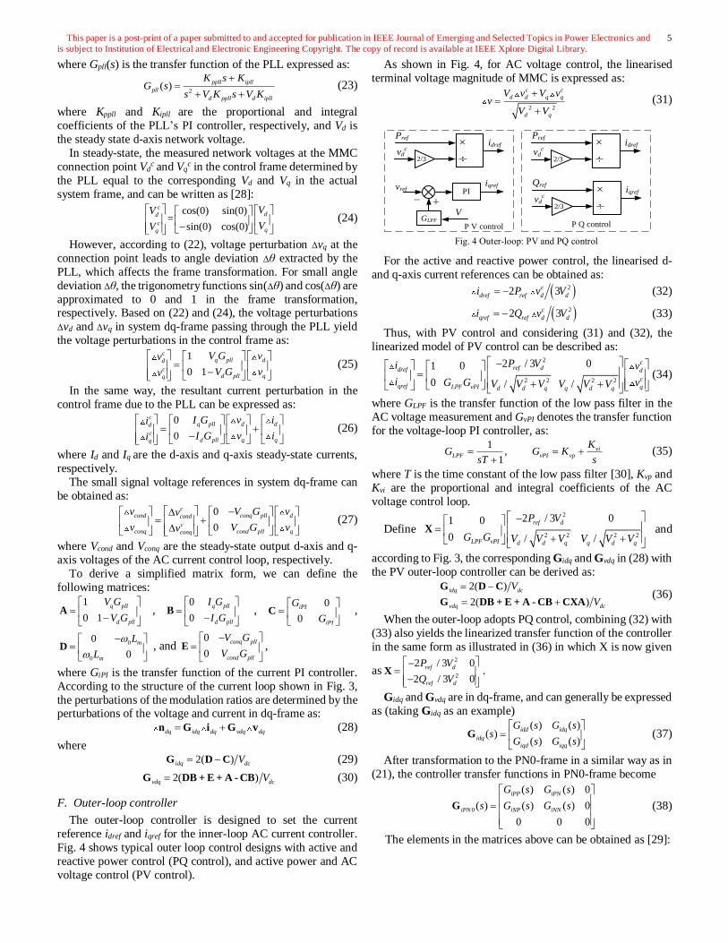
Fig. 6 compares the admittance elements YPP(s) and YPN(s) in

matrix YMMC derived from the HSS model with different

harmonic orders considered, and those obtained from the time-

domain model. The MMC exports 1000MW / 0MVar to the AC

grid and the AC terminal voltage is 1 pu. Open-loop control is considered and the 3-phase modulations for the arms are the

same as in Section Ⅳ A. The other two elements in YMMC,

YNP(s-2jω0), and YNN(s-2jω0), have similar trends and due to

space limit, are not presented here. Comparing the different

admittance curves, it can be found that higher harmonic order

considered in the analytical HSS model leads to more accurate

model, and for h=4 the analytical admittances match well with

those of the time-domain simulation models. It also implies that

the internal harmonics of MMC has a significant impact on the

AC side small-signal admittance, and need to be considered in

the modelling.

0 50 100 150 200 250 300Frequency (Hz)

0

10

20

30FFT Analysis Result

i ga (

A)

0 50 100 150 200 250 300Frequency (Hz)

0

1000

2000


vga (

V)

0 50 100 150 200 250 300

Frequency (Hz)

0

20

40


i ga (

A)

0 50 100 150 200 250 300Frequency (Hz)

0

1000

2000


vga (

V)



8

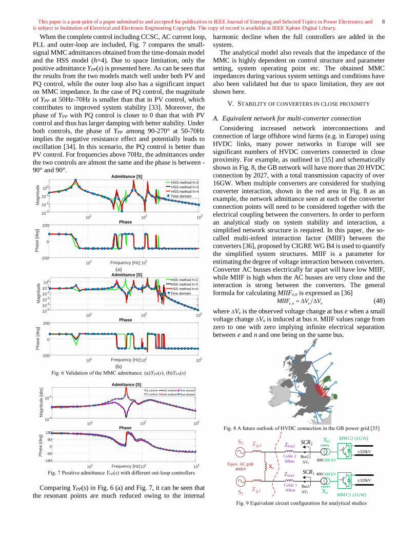
When the complete control including CCSC, AC current loop,

PLL and outer-loop are included, Fig. 7 compares the small-

signal MMC admittances obtained from the time-domain model

and the HSS model (h=4). Due to space limitation, only the

positive admittance YPP(s) is presented here. As can be seen that the results from the two models match well under both PV and

PQ control, while the outer loop also has a significant impact

on MMC impedance. In the case of PQ control, the magnitude

of YPP at 50Hz-70Hz is smaller than that in PV control, which

contributes to improved system stability [33]. Moreover, the

phase of YPP with PQ control is closer to 0 than that with PV

control and thus has larger damping with better stability. Under

both controls, the phase of YPP among 90-270° at 50-70Hz

implies the negative resistance effect and potentially leads to

oscillation [34]. In this scenario, the PQ control is better than

PV control. For frequencies above 70Hz, the admittances under

the two controls are almost the same and the phase is between -90° and 90°.

101

102

103

10-3

10-2

10-1

100

Mag

nitude

Admittance [S]

101

102Frequency [Hz]

-200

0

200

Phase

[deg

]

Phase

HSS method h=2

HSS method h=3

HSS method h=4

Time domain

(a)

101

102

103

10-5

10-4

10-3

10-2

10-1

100

Mag

nitude

Admittance [S]

101

102

103Frequency [Hz]

-200

0

200

Phase

[deg

]

Phase

HSS method h=2

HSS method h=3

HSS method h=4

Time domain

(b)

Fig. 6 Validation of the MMC admittance. (a)YPP(s), (b)YPN(s)

Fig. 7 Positive admittance YPP(s) with different out-loop controllers

Comparing YPP(s) in Fig. 6 (a) and Fig. 7, it can be seen that

the resonant points are much reduced owing to the internal

harmonic decline when the full controllers are added in the

system.

The analytical model also reveals that the impedance of the

MMC is highly dependent on control structure and parameter

setting, system operating point etc. The obtained MMC impedances during various system settings and conditions have

also been validated but due to space limitation, they are not

shown here.

V. STABILITY OF CONVERTERS IN CLOSE PROXIMITY

A. Equivalent network for multi-converter connection

Considering increased network interconnections and

connection of large offshore wind farms (e.g. in Europe) using

HVDC links, many power networks in Europe will see

significant numbers of HVDC converters connected in close

proximity. For example, as outlined in [35] and schematically

shown in Fig. 8, the GB network will have more than 20 HVDC

connection by 2027, with a total transmission capacity of over

16GW. When multiple converters are considered for studying

converter interaction, shown in the red area in Fig. 8 as an example, the network admittance seen at each of the converter

connection points will need to be considered together with the

electrical coupling between the converters. In order to perform

an analytical study on system stability and interaction, a

simplified network structure is required. In this paper, the so-

called multi-infeed interaction factor (MIIF) between the

converters [36], proposed by CIGRE WG B4 is used to quantify

the simplified system structures. MIIF is a parameter for

estimating the degree of voltage interaction between converters.

Converter AC busses electrically far apart will have low MIIF,

while MIIF is high when the AC busses are very close and the interaction is strong between the converters. The general

formula for calculating MIIFe,n is expressed as [36]

,e n e nMIIF V V= (48)

where ΔVe is the observed voltage change at bus e when a small

voltage change ΔVn is induced at bus n. MIIF values range from

zero to one with zero implying infinite electrical separation

between e and n and one being on the same bus.

Fig. 8 A future outlook of HVDC connection in the GB power grid [35]

MMC2 (1GW)

MMC1 (1GW)

Equiv. AC grid

400kV

Zline2

Xc

Zg 1

Zg 2

Xt2

Xt1

Zline1

S2

S1

SCR2

400/360 kV

±320kV

±320kV

Cable 2

60km

Cable 1

60km

400/360 kVSCR1

Bus2

Bus1

ΔV2

ΔV1

Fig. 9 Equivalent circuit configuration for analytical studies

101

102

103

10-4

10-2

Mag

nitude

[abs]

Admittance [S]

101

102

103Frequency [Hz]

-180

-90

0

90

180

Phase

[deg

]

Phase

HSS method Time domain

HSS method Time domain

PQ control：

PV control：



9

Considering the case with two MMCs, each of the MMC can

be equivalent to connection with an AC source through a certain

impedance to emulate the network condition at the MMC

connection point, and the two AC sources are interconnected

(within the same AC network). Thus, a simplified network configuration as shown in Fig. 9 can be developed. Zline1 and

Zline2 in Fig. 9 are considered as the impedances for two 60km

cables connecting the MMCs to the existing network. The

interconnection between the two AC sources is represented by

a value of Xc considering the high X/R ratio in transmission

systems. Applying the MIIF concept, the followings are

considered when setting the network parameters:

• MMC1 infeed is considered as an existing HVDC link, and

thus Zg1 is pre-determined.

• When there exists strong electrical coupling between MMC1

and MMC2, i.e. the two converters are in close proximity (high MIIF), Xc is set to a low value while Zg2 is set to a high

value, so that MMC2 can be deemed close to AC system S1

while being further away from S2.

• When there only exists weak electrical coupling between

MMC1 and MMC2 (low MIIF), Xc is set to a high value

while Zg2 is set to a low value, so that MMC2 can be deemed

close to AC system S2 and far away from S1.

Accordingly, the specific network parameters for cases of

weak and strong coupling are given in Table III. The equivalent

impedances of the AC grids are Zg1=Rg1+jω0Lg1 and

Zg2=Rg2+jω0Lg2, and Xc=jω0Lc is the reactance for

interconnecting the two grids. By varying Zg1, Zg2, and Xc, different infeed conditions, i.e., electrical distances, can be

emulated. Based on the parameters in Table III, the

corresponding SCR for weak and strong couplings are

presented in Table IV.

Table III System parameter for weak coupling and strong coupling

Parameters Weak coupling Strong coupling

Lt1 and Lt2 0.0587H 0.0587H

Length of Cable1 & 2 60 km 60 km

Rg1 / Lg1 4.08Ώ / 0.1296H 4.08Ώ / 0.1296H

Rg2 / Lg2 4.08Ώ / 0.1296H 10.2 Ώ / 0.324H

Lc 0.3H 0.01H

Table IV SCR and MIIF in the case of weak coupling and strong coupling

Weak coupling Strong coupling

SCR1 /SCR2 2.59 / 2.59 2.74 / 2.64

MIIF1,2 / MIIF2,1 0.26 / 0.26 0.78 / 0.81

Considering the voltages for sources S1 and S2 are the same,

the network can be further simplified by combining the two

sources into one with the three delta-connected impedance

Zg1(s), Zg2(s), and Xc(s) transformed to equivalent Y connection as shown in Fig. 10. Note that Zg1, Zg2 and Xc are diagonal 2 by

2 impedance matrix in PN0-frame for the 3-phase balanced

system [12].

B. Stability assessment of converters in close proximity

As shown in Fig. 10, the equivalent AC external impedance

Zeg1(s) at MMC1 can be derived as

1 3 2 2 2 2

1 1 1

( ) [ ( ) ( ( ) ( ) ( ) ( )]

( ) ( ) ( )

Z Z Z Z X Z

Z Z X

eg e e line t MMC

e line t

s s s s s s

s s s

= + + +

+ + + (49)

According to [33], in order to use Nyquist stability criteria,

the system has to meet the following conditions:

• MMC1 and MMC2 are stable when they are individually

and directly connected to ideal voltage sources.

• The grid voltage is stable without MMC1 and MMC2

connection.

The above conditions are met in a normal electrical network setup, and the matrices Zeg1(s) and YMMC1(s) do not have right-

half-plane (RHP) poles. Thus, the system stability can be

assessed based on Nyquist curve for eigenvalue loci of the

matrix Zeg1(s)YMMC1(s). Both MMC1 and MMC2 adopt the same

control shown in Fig. 2 and Fig. 3, and also have the same outer-

loop PQ control with both active references being 1GW. The

reactive power of the MMCs are set to maintain their terminal voltages at 400kV, and the control parameters are listed in

Table V.

Zline2(s)

Zline1(s)

ZMMC2(s)

Xt2(s)

Xt1(s)

YMMC1(s)

Ze2(s)

Ze1(s)

Ze3(s)

Zeg1(s)

Fig. 10 Small-signal impedance equivalent circuit

Table V Controller parameters for MMC controller

Parameters Value

Current loop PI gains: Kip , Kii 15.8 Ω, 2980 Ω/s

PLL PI gains: Kpllp , Kplli 0.0013rad/(sV), 0.12rad/(s2V)

CCSC PR controller gains: Krp , Krr 63.3 Ω, 11200 Ω/s

AC voltage controller PI gains: Krp , Kri 0.005 A/V, 0.5A/ (s·V)

-1.5 -1 -0.5 0 0.5 1 1.5-1.5

-1

-0.5

0

0.5

1

1.5 1 High MIIF

2 High MIIF

(-1,0)

unit circle

66Hz

(a) with low MIIF (b) with high MIIF

Fig. 11 Nyquist plots for different MIIF using PQ control

Under different MIIF, the Nyquist plots for eigenvalue loci

of Zeg1(s)YMMC1(s) are compared in Fig. 11. For both MIIF

cases, the eigenvalue locus do not encircle the point (−1, 0) and thus the system is stable. As described in [37], the phase and

gain margins can also be observed based on the Nyquist plots.

With low MIIF (MIIF2,1=0.26 in this example), the interaction

of the two MMCs are weak and the Nyquist plots imply that the

system has sufficient phase margin and magnitude margin and

thus system stability is strong. In the case of high MIIF

(MIIF2,1=0.81 in this example), the system stability is weakened

with low gain margin and phase margin. Meanwhile, the

crossover frequency of the Nyquist curve shown in Fig. 11(b)

is 66Hz, indicating the system has the worst stability around

66Hz, which is in the frequency range of MMC negative resistance appearing in Fig. 7. However, it needs to be noted

that MMC negative resistance itself will not necessarily lead to

unstable system as stability is the result of the interaction of

multiple impedances including network.

-1.5 -1 -0.5 0 0.5 1 1.5-1.5

-1

-0.5

0

0.5

1

1.5 1 Low MIIF

2 Low MIIF

(-1,0)

unit circle



10

The corresponding time-domain simulation results are given

in Fig. 12. At 12s, a small perturbation is injected into the active

power reference of MMC1. The d-axis current of MMC1 with

low MIIF has smaller overshoot and can reach stable operation

quicker than that under high MIIF as seen in Fig. 12 (a) and (b), indicating the system under low MIIF has higher stability

margin than that under high MIIF. Note that the oscillation

frequency in Fig. 12 (b) is around 16Hz in dq-frame,

corresponding to 66 Hz in AC system. The simulation results

thus accord well with the Nyquist analysis.

(a) Low MIIF (b) High MIIF

Fig. 12 The d-axis current of MMC1 with different MIIF

The effect of different outer-loop control on the stability of

the interconnection system is further investigated. MMC1 now

adopts PQ control and MMC2 PV control. Under different

MIIF, the Nyquist plots are depicted in Fig. 13. As can be seen,

with low MIIF, the system can maintain sufficient stability,

whereas with high MIIF, the system becomes unstable. The

corresponding time-domain simulation results shown in Fig. 14

match well with that of Fig. 13, in which the system is unstable

for high MIIF. Further studies considering different MIIF and

outer-loop controllers reveal similar results. When multiple

converters are considered, a system with low MIIF has better system stability than that with high MIIF, and outer-loop can

also significantly impact on system stability. However, a clear

boundary between high and low MIIF is difficult to define and

full system studies are required to determine system stability.


Fig. 13 Nyquist plots with PQ and PV control.


Fig. 14 The d-axis current of MMC1 with different MIIF.

Looking into the causes of the reduced stability margin in

Fig. 11(b) and instability in Fig. 13(b), the negative resistance

in the MMC admittance in the frequency range of 50-70Hz is of clear concern. This in combination with the high admittance

magnitude under PV control leads to instability as shown in Fig.

13(b) and Fig. 14(b). Therefore, parameter turning or additional

voltage control to reduce the admittance magnitude within 50-

70Hz under PV control can likely improve system stability.

Further studies and results will be report in the future.

When assessing system stability, converters including wind

farms, HVDC, FACTS etc. connected in close proximity to the

point of common coupling must be fully considered. In addition, converter admittance is affected by its operating point

as previously described. Thus, the assessment of multiple

converter interaction is a complex issue which is affected by

multiple factors including the states and operation of the

network and converters etc.

VI. CONCLUSION

This paper has described the impedance modelling and

validation of the three-phase MMC converter based on HSS. The detailed mathematical expressions for HSS modelling for

MMC have been derived considering the integration of various

inner and outer control loops. The coupling between the

positive and negative sequence components brought by external

control loops and PLL are analyzed in the model. The small-

signal impedances obtained from the developed analytical

model have been validated using time-domain models. With the

impedance model, the interaction of multiple converters in

close proximity is studied considering different multi-infeed

interaction factor (MIIF). Stability analysis and time domain

simulation results show good match and that system with high MIIF where strong couplings between the two MMCs exist may

cause the instability of the system.

Converter and system impedances are highly dependent on

operating point, controller setting, and network structure, and

thus further studies to investigate the impact of their variations

on system stability are required. In addition, to identify states

where the risk of instability may exist in a multi-infeed

converter system is critical, so as to help inform operating away

from those network or converter operating states.

APPENDIX A

The matrices in (14) are given as

0 1

1

0 1

1 0 1

1 0

1

1 0

h

s s s

s

s s

h hs s s s s s

s s

s

h

s s s

− −

−

− −

−

=

A A A

A

A A

A A A A A A

A A

A

A A A

0 1

1

0 1

1 0 1

1 0

1

1 0

h

h h

h

− −

−

− −

−

=

B B B

B

B B

B B B B B B

B B

B

B B B

-2 -1 0 1-1.5

-1

-0.5

0

0.5

1

1.5 1 Low MIIF

2 Low MIIF

(-1,0)

-2 -1 0 1-1.5

-1

-0.5

0

0.5

1

1.5 1 High MIIF

2 High MIIF

(-1,0)



11

0 1

1

0 1

1 0 1

1 0

1

1 0

h

h h

h

− −

−

− −

−

=

M M M

M

M M

M M M M M M

M M

M

M M M

0

0

0

0

( )

( )

= ( )

( )

( )

s jh

s j

s

s j

s jh

−

− +

+

A

A

A A

A

A

G

G

HG G

G

G

0

0

0

0

( )

( )

= ( )

( )

( )

s jh

s j

s

s j

s jh

−

− +

+

B

B

B B

B

B

G

G

HG G

G

G

0

0

0

0

= 0

jh

j

j

jh

−

−

I

I

Q I

I

I

0 0 0 0

0 0 0 0

0 0 0 0

0 0 0 0

0 0 0 0

( ) ( )

( ) ( )

= ( ) , = ( )

( ) ( )

( ) ( )

PN PN

PN PN

PN PN PN PN

PN PN

PN PN

s jh s jh

s j s j

s s

s j s j

s jh s jh

− − − − + + + +

Δx Δv

Δx Δv

ΔX Δx ΔV Δv

Δx Δv

Δx Δv

REFERENCES

[1] H. Saad, Y. Fillion, S. Deschanvres, Y. Vernay, and S. Dennetière, “On

resonances and harmonics in HVDC-MMC station connected to AC grid,”

IEEE Trans. Power Del., vol. 32, no. 3, pp. 1565–1573, Jun. 2017.

[2] A. Beddard, C. E. Sheridan, M. Barnes, and T. C. Green, “Improved

accuracy average value models of modular multilevel converters,” IEEE

Trans. Power Del., vol. 31, no. 5, pp. 2260–2269, Oct. 2016.

[3] H. Yang, Y. Dong, W. Li, and X. He, “Average-value model of modular

multilevel converters considering capacitor voltage ripple,” IEEE Trans.

Power Del., vol. 32, no. 2, pp. 723–732, Apr. 2017.

[4] J. Dorn, H. Huang, and D. Retzmann, “A new multilevel voltage-sourced

converter topology for HVDC applications,” in Proc. CIGRE, Paris,

France, Aug. 24–29, 2008, pp. 1–8.

[5] S. Shah, “Small and large signal impedance modelling for stability

analysis of grid-connected voltage source converters,” Department of

Electrical Engineering, Rensselaer Polytechnic Institute, Troy, New York,

2018.

[6] A. Nami, J. Liang, F. Dijkhuizen, and G. D. Demetriades, “Modular

multilevel converters for HVDC applications: Review on converter cells

and functionalities,” IEEE Trans. Power Electron., vol. 30, no. 1, pp. 18–

36, Jan. 2015.

[7] A. Jamshidifar, and D. Jovcic, “Small-signal dynamic dq model of

modular multilevel converter for system studies,” IEEE Trans. Power

Del., vol. 31, no. 1, pp. 1991–1999, Feb. 2016.

[8] Y. Li, G. Tang, J. Ge, Z. He, H. Pang, J. Yang, and Y. Wu, “Modelling

and damping control of modular multilevel converter based dc grid,”

IEEE Trans. Power Syst., vol. 31, no. 1, pp. 723–735, Jan. 2018.

[9] J. Lyu, X. Cai, and M. Molinas, “Frequency domain stability analysis of

MMC-based HVDC for wind farm integration,” IEEE J. Emerg.

Sel.Topics Power Electron., vol. 4, no. 1, pp. 141–151, Mar. 2016.

[10] M. Beza, M. Bongiorno, and G. Stamatiou, “Analytical derivation of the

ac-side input admittance of a modular multilevel converter with open- and

closed-loop control strategies,” IEEE Trans. Power Del., vol. 33, no. 1,

pp. 248–256, Feb. 2018.

[11] L. Bessegato, K. Ilves, L. Harnefors, and S. Norrga, “Effects of control

on the ac-side admittance of a modular multilevel converter”, IEEE Trans.

Power Electron., vol. 34, no. 8, pp. 7206–7220, Aug. 2019.

[12] S. Hwang, “Harmonic state-space modelling of an hvdc converter with

closed-loop control,” Department of Electrical and Computer Engineering，

University of Canterbury, Christchurch, New Zealand，2013.

[13] J. J. Rico, M. Madrigal and E. Acha, “Dynamic harmonic evolution using

the extended harmonic domain,” IEEE Trans. Power Del., vol. 18, no. 2,

pp. 587-594, April 2003.

[14] J. J. Chavez and A. Ramirez, “Dynamic Harmonic Domain Modelling of

Transients in Three-Phase Transmission Lines,” IEEE Trans. Power Del.,

vol. 23, no. 4, pp. 2294-2301, Oct. 2008.

[15] J. B. Kwon, X. Wang, F. Blaabjerg, C. L. Bak, A. R. Wood and N. R.

Watson, “Harmonic instability analysis of a single-phase grid-connected

converter using a harmonic state-space modelling method,” IEEE Trans.

Ind. Appl., vol. 52, no. 5, pp. 4188-4200, Sept.-Oct. 2016.

[16] J. Lyu, X. Zhang, X. Cai, and M. Molinas, “Harmonic state-space based

small-signal impedance modelling of modular multilevel converter with

consideration of internal harmonic dynamics,” IEEE Trans. Power

Electron., vol. 34, no. 3, pp. 2134–2148, Mar. 2019.

[17] Z. Xu, B. Li, S. Wang, S. Zhang and D. Xu, “Generalised Single-Phase

Harmonic State Space Modelling of the Modular Multilevel Converter

With Zero-Sequence Voltage Compensation,” IEEE Trans. Ind. Electron.,

vol. 66, no. 8, pp. 6416-6426, Aug. 2019.

[18] H. Wu, X. Wang and Ł. Kocewiak, “Impedance-Based Stability Analysis

of Voltage-Controlled MMCs Feeding Linear AC Systems,” IEEE J.

Emerg. Sel. Topics Power Electron., early access, 2019.

[19] H. Wu and X. Wang, “Dynamic Impact of Zero-Sequence Circulating

Current on Modular Multilevel Converters: Complex-Valued AC

Impedance Modelling and Analysis,” IEEE J. Emerg. Sel. Topics Power

Electron., vol. 8, no. 2, pp. 1947-1963, June 2020.

[20] A. Rygg, M. Molinas, C. Zhang and X. Cai, “A Modified Sequence-

Domain Impedance Definition and Its Equivalence to the dq-Domain

Impedance Definition for the Stability Analysis of AC Power Electronic

Systems,” IEEE J. Emerg. Sel. Topics Power Electron., vol. 4, no. 4, pp.

1383-1396, Dec. 2016.

[21] H. Zong, J. Lyu, C. Zhang, X. Cai, M. Molinas and F. Rao, “MIMO

impedance based stability analysis of DFIG-based wind farm with MMC-

HVDC in modified sequence domain,” in Proc. 8th Int. Conf. Renew.

Power Gener. (RPG), Shanghai, China, 2019, pp. 1-7.

[22] H. Zong, C. Zhang, J. Lyu, X. Cai, M. Molinas and F. Rao, “Generalized

MIMO Sequence Impedance Modeling and Stability Analysis of MMC-

HVDC With Wind Farm Considering Frequency Couplings,” IEEE

Access, vol. 8, pp. 55602-55618, 2020.

[23] K. Ji, G. Tang, H. Pang and J. Yang, "Impedance Modeling and Analysis

of MMC-HVDC for Offshore Wind Farm Integration," IEEE Trans.

Power Del., vol. 35, no. 3, pp. 1488-1501, June 2020.

[24] R. Li, L. Xu and D. Guo, “Accelerated switching function model of hybrid

MMCs for HVDC system simulation,” IET Power Electron., vol. 10, no.

15, pp. 2199-2207, 15 12 2017.

[25] D. Guo, M. H. Rahman, G. P. Ased, L. Xu, A. Emhemed, G. Burt, et al.,

“Detailed quantitative comparison of half-bridge modular multilevel

converter modelling methods,” The Journal of Engineering, vol. 2019, pp.

1292-1298, 2019. [26] J. Sun, “Small-Signal Methods for AC Distributed Power Systems–A

Review,” IEEE Trans. Power Electron., vol. 24, no. 11, pp. 2545-2554,

Nov. 2009.

[27] D. N. Zmood and D. G. Holmes, “Stationary frame current regulation of

PWM inverters with zero steady-state error,” IEEE Trans. Power

Electron., vol. 18, no. 3, pp. 814-822, May. 2003.

[28] B. Wen, D. Boroyevich, R. Burgos, P. Mattavelli, and Z. Shen, “Analysis

of D-Q small-signal impedance of grid-tied inverters,” IEEE Trans.

Power Electron., vol. 31, no. 1, pp. 675–687, Jan. 2016.

[29] G. Amico, A. Egea-Àlvarez, P. Brogan and S. Zhang, “Small-signal

converter admittance in the pn-frame: systematic derivation and analysis

of the cross-coupling terms,” IEEE Trans. Energy Conver., vol. 34, no. 4,

pp. 1829-1838, Dec. 2019.



12

[30] O. Katsuhiko and Y. Yang, Modern Control Engineering, 5ed. Upper

Saddle River, NJ: Prentice hall, 2010.

[31] J. Sun and H. Liu, “Sequence Impedance Modelling of Modular

Multilevel Converters,” IEEE J. Emerg. Sel. Topics Power Electron., vol.

5, no. 4, pp. 1427-1443, Dec. 2017.

[32] M. Cespedes and J. Sun, “Impedance Modelling and Analysis of Grid-

Connected Voltage-Source Converters,” IEEE Trans. Power Electron.,

vol. 29, no. 3, pp. 1254-1261, March. 2014.

[33] J. Sun, “Impedance-based stability criterion for grid-connected inverters,”

IEEE Trans. Power Electron., vol. 26, no. 11, pp. 3075–3078, Nov. 2011.

[34] M. Cespedes, L. Xing and J. Sun, “Constant-power load system

stabilisation by passive damping,” IEEE Trans. Power Electron., vol. 26,

no. 7, pp. 1832-1836, July 2011.

[35] “GB National Electricity System Seven Year Statement”, National Grid,

2011.

[36] B. Davies et al., Systems with multiple dc infeed, CIGRE Working Group

B4.41, Paris, France, pp. 12–14, Dec. 2008.

[37] L. Harnefors, “Modeling of Three-Phase Dynamic Systems Using

Complex Transfer Functions and Transfer Matrices,” IEEE Trans. Ind.

Electron., vol. 54, no. 4, pp. 2239-2248, Aug. 2007.

Yin Chen received the B.S. degree in electrical

engineering from Huazhong University of Science and

Technology, Wuhan, China, in 2009, and the M.S.

degree in electrical engineering from Zhejiang

University, Hangzhou, China, in 2014. He received the

Ph.D. degree in Electrical Engineering from University

of Strathclyde, Glasgow, U.K. in 2020.

He is currently a post-doctoral researcher with

University of Strathclyde in Glasgow, UK. His research

interests include modelling of power electronic

converters, grid integration of renewable power, and stability analysis of the

HVDC transmision systems.

Lie Xu (M’03–SM’06) received the B.Sc. degree in

Mechatronics from Zhejiang University, Hangzhou,

China, in 1993, and the Ph.D. degree in Electrical

Engineering from the University of Sheffield,

Sheffield, UK, in 2000.

He is currently a Professor at the Department of

Electronic & Electrical Engineering, University of

Strathclyde, Glasgow, UK. He previously worked in

Queen’s University of Belfast and ALSTOM T&D,

Stafford, UK. His current research interests include

power electronics, wind energy generation and grid integration, and application

of power electronics to power systems such as HVDC and MVDC systems for

power transmission and distribution. He is an Editor of IEEE Transactions on

Power Delivery and IEEE Transactions on Energy Conversion.

Agustí Egea-Àlvarez (S’12–M’14) obtained his B.Sc,

MSc and Ph.D. from the Technical University of

Catalonia in Barcelona in 2008, 2010 and 2014

respectively. In 2015 he was a Marie Curie fellow in

the China Electric Power Research Institute (CEPRI).

In 2016 he joined Siemens Gamesa as converter

control engineer working on grid forming controllers

and alternative HVDC schemes for offshore wind

farms. Currently, Dr Agust Egea-lvarezis Strathclyde

Chancellors fellow (Lecturer) at the electronic &

electrical engineering department and member of the

PEDEC (Power Electronics, Drives and Energy Conversion) group since 2018.

He is a member of IEEE, IET and has been involved in several CIGRE and

ENTSO-E working groups.

His current research interests include control and operation of high-voltage

direct current systems, renewable generation systems, electrical machines and

power converter control.

Benjamin Marshall is currently the HVDC

Technology Manager at the UK National HVDC

Centre. Ben oversees the team of Simulation Engineers

undertaking detailed HVDC simulation studies in real-

time using vendor-supplied replica hardware, to

understand multi-infeed, multi-terminal and multi-

vendor HVDC operation and interactions, for real

schemes in GB; interpreting the results to gain insights

to improve the design and operation of HVDC schemes.

Ben previously has had a 23 year long and varied

career within National Grid with a broad range of experience, particularly with

respect to the analysis of the operation and design of the AC and DC

transmission systems. He has experience in both offline and real-time EMT

simulation and in modelling of convertors across battery, solar wind and HVDC

systems, He has developed deep technical skills relating to dynamic stability of

power systems and the performance specification of HVDC convertors. Within

the ESO, Ben advised on the specification, validation and modelling of new

HVDC connections, supporting the compliance connection planning and

requirements and provided technical leadership on AC and DC control systems,

System Operability, Smart Grids and power system simulation; leading

complex power system studies.

Md Habibur Rahman obtained B.Sc. degree in

Electrical and Electronic Engineering from

Ahsanullah University of Science and Technology,

Bangladesh in 2007, and in 2011 he received his

M.Sc. degree in Sustainable Electrical Power from

Brunel University, UK. Since 2014 has been a PhD

researcher with the Department of Electronic and

Electrical Engineering at the University of

Strathclyde, UK.

He is currently a simulation engineer at the

National HVDC Centre, UK. His research interest is mainly focused on Multi-

terminal HVDC system concentrating on fault management, design of

converters for HVDC applications, protection schemes and control of power

electronics. He is an active contributor to the reviewing process of IEEE and

IET Transactions and conferences and a member of IEEE and IET.

Oluwole Daniel Adeuyi (S’11–M’16) received the

B.Sc. degree in electrical/electronic engineering

from the Federal University of Agriculture,

Abeokuta, Nigeria, in 2010, the M.Sc. degree

(Hons.) in 2012, and the Ph.D. degree in electrical

energy system in 2016, both from Cardiff

University, U.K, where he worked as a

postdoctoral research associate with focus on

control and operation of HVDC-connected wind

farms. In 2018, he joined the National HVDC

Centre (part of SSEN Transmission) and has supported de-risking industrial

HVDC schemes for integration of renewable energy systems.

Documents

is subject to Institution of Electrical and Electronic