Embed Size (px)
Citation preview
1
Is The Phillips Curve Alive and Well After All? Inflation Expectations and the Missing Disinflation
Olivier Coibion Yuriy Gorodnichenko UT Austin and NBER
UC Berkeley and NBER
This draft: September 30th, 2013
Abstract: We evaluate possible explanations for the absence of a persistent decline in inflation during the Great Recession and find commonly suggested explanations to be insufficient. We propose a new explanation for this puzzle within the context of a standard Phillips curve. If firms’ inflation expectations track those of households, then the missing disinflation can be explained by the rise in their inflation expectations between 2009 and 2011. We present new econometric and survey evidence consistent with firms having similar expectations as households. The rise in household inflation expectations from 2009 to 2011 can be explained by the increase in oil prices over this time period.
JEL Codes: E3, E5 Keywords: deflation, Phillips curve, expectations
Acknowledgements: We thank Larry Ball, Mark Gertler, Andy Levin, and Troy Matheson for very helpful comments, Graham Howard for assistance with data from the Reserve Bank of New Zealand, and Saten Kumar for survey data on firms’ inflation forecasts. This paper was written in part while Coibion was a visiting scholar at the IMF, whose support was greatly appreciated. The views expressed in the paper are those of the authors and should not be interpreted as representing those of any institutions with which they are or have been affiliated. Gorodnichenko thanks NSF and Sloan Foundation for financial support.
2
“Prior to the recent deep worldwide recession, macroeconomists of all schools took a negative relation between slack and declining inflation as an axiom. Few seem to have awakened to the recent experience as a contradiction to the axiom.” Bob Hall (2013) I Introduction
During the Great Depression, the United States experienced devastating levels of deflation - more than 10
percent per year in 1932. Japan was mired in borderline deflation territory from the mid-1990s through
mid-2000s after its real estate and stock market bubbles popped in the early 1990s. But advanced economies
have experienced little decline in inflation since the financial crisis of 2008-2009, calling into question one
of the fundamental tenets of many macroeconomic theories: the Phillips curve linking the rate of change in
prices to the level of economic activity.
While economists have suggested a number of possible explanations for the “missing disinflation”,
we argue that these appear insufficient to explain the full extent of the inflation experience of recent years.
For example, the “anchored expectations” hypothesis of Bernanke (2010)—that is, the credibility of modern
central banks has convinced people that neither high inflation nor deflation are likely outcomes thereby
stabilizing actual inflation outcomes through expectational effects—can only go some way in accounting
for the absence of more significant disinflation between 2009 and 2011. Explanations based on recent labor
market developments, such as long-term unemployed having smaller effects on wages (Llaudes 2005) or
downward wage rigidity preventing wages from falling as much as in prior downturns (Daly, Hobijn and
Lucking 2012), imply that the missing disinflation in prices should have been accompanied by a missing
disinflation in wages, a feature which we show is noticeably absent in the data. Others have pointed to a
flattening Phillips curve (IMF 2013), but the statistical evidence for this explanation is delicate, no structural
changes in the economy can account for the required change in the slope of the Phillips curve, and the
quantitative effects of the estimated changes in the slope are themselves insufficient to account for much
of the missing disinflation. This inability to explain the missing disinflation within the context of the Phillips
curve has led some to conclude that this framework may have outlived its usefulness.
We instead propose a novel explanation for the missing disinflation that remains fully within the
context of traditional Phillips curve analysis. Specifically, we show that an expectations-augmented Phillips
curve, using household inflation expectations as measured by the Michigan Survey of Consumers, can
account for the absence of strong disinflationary pressures since 2009. The primary reason for the success
of a household inflation expectation-augmented Phillips curve is that household inflation expectations
experienced a sharp rise starting in 2009, going from a low of 2.5% to around 4% in 2013, whereas other
measures of inflation expectations such as those from financial markets or professional forecasters have
hovered in the close neighborhood of 2% over the same period.
3
Why focus on the expectations of households in the context of the Phillips curve, since the latter is
meant to capture the pricing decisions, and therefore expectations, of firms? First, there is no quantitative
measure of firm inflation expectations available in the U.S., so that the question of how firms form their
inflation expectations, and what may be the best proxy for them, is ex-ante ambiguous. Given that many
prices are set by small and medium-sized enterprises who do not have professional forecasters on staff (and
who likely have little to gain from purchasing professional forecasting services), it seems a priori as likely
for their inflation expectations to be well-proxied by household forecasts as by professional forecasts.
Second, we present empirical evidence from estimated Phillips curves in the pre-Great Recession period
that household forecasts are indeed likely to be a better proxy for firm forecasts than either professional or
backward-looking forecasts. Specifically, regressions which include both household and professional
forecasts systematically point to a larger role for household forecasts than any other measure of inflation
expectations. Third, we present preliminary results from an ongoing survey of firms’ inflation expectations
in New Zealand and show that their properties are much more similar to those of households than to
professional forecasts, with relatively high levels of forecasted inflation and very high dispersion of
inflation forecasts across firms, in line with household forecasts but strongly at odds with professional
forecasts. Thus, the available evidence is consistent with the use of household inflation forecasts as a proxy
for firm forecasts of inflation in the Phillips curve.
We then consider the source of the rise in household inflation expectations relative to the forecasts
of professional forecasters since 2009, which is the main feature of the data which accounts for the missing
disinflation. We document that more than half of the historical differences in inflation forecasts between
households and professionals can be accounted for by the level of oil prices. With oil prices having risen
sharply since 2009, this provides a quantitatively successful explanation for the rise in household inflation
expectations. Why would households adjust their inflation forecasts more strongly in response to oil price
changes than professional forecasters? Because gasoline prices are among the most visible prices to
consumers, a natural explanation could be that households pay particular attention to them when
formulating their expectations of other prices. Consistent with this notion, we document using the micro-
data from the Michigan Survey of Consumers that individuals who on average spend more money on
gasoline (in dollar terms) and therefore frequent gas stations more often adjust their inflation forecasts by
more in response to oil price changes than do individuals who spend less money on gasoline.
Our suggested explanation for the missing disinflation has several appealing properties. First, it fits
naturally within the Phillips curve framework. Second, it is quantitatively successful in explaining the
absence of disinflation. Third, we present new econometric and survey evidence consistent with firms’
inflation expectations being well-proxied by those of households. Fourth, the difference in household
inflation expectations and those of professional forecasters since 2009 can readily be accounted for by the
4
evolution of oil prices during this period. Finally, our explanation is consistent with the absence of strong
deflationary pressures across a wide range of advanced economies since the recent financial crisis (IMF
2013), which supports explanations based on common factors such as oil price movements.
One unusual implication of our explanation is that the absence of more pronounced disinflation –
or even deflation- in advanced economies following the Great Recession likely reflected a unique set of
factors (e.g. rapid recoveries in developing economies like China spurring global demand for commodities,
as in Kilian and Murphy 2012) which policymakers should not necessarily expect to be repeated in future
crises. And to the extent that this rise in inflationary expectations may have prevented the onset of
pernicious deflationary dynamics, the rise in oil prices should perhaps be interpreted as a lucky break for
policymakers, generating the very rise in inflationary expectations which policymakers have only recently
begun to push aggressively toward in the form of forward guidance.
A second unusual feature of this interpretation is that, contrary to Bernanke’s “anchored
expectations” hypothesis, we rely on the fact that household expectations have not been fully anchored and
continue to respond strongly to commodity price changes to explain the missing disinflation. If our
explanation is correct, anchored expectations on the part of households and firms would likely have
delivered much worse economic outcomes through more pronounced disinflationary dynamics. So while
anchored expectations likely remain a desirable outcome in most circumstances, the experience since 2009
presents a cautionary example of the potential downside of fully anchored expectations.
Our paper builds on a long literature on the expectations-augmented Phillips curve, in the spirit of
Friedman (1968). This literature has identified a number of potential issues regarding the estimation and
interpretation of Phillips curve relationships. We address some of these concerns in the paper, such as the
importance of using real-time expectations (Roberts 1998), the sensitivity of inflation to marginal costs
(Gali and Gertler 1999), the possibility of asymmetries due to downward wage rigidities (Akerlof et al.
1996), and the sensitivity to trend inflation (Ascari and Ropele 2007). But some other concerns are not
directly addressed, including the degree of price and wage indexation (Christiano, Eichenbaum and Evans
2005), the nature of pricing rigidities, such as Calvo (1983) vs. Taylor (1982) or state-dependent price
setting (Dotsey, King and Wolman 2003, Gorodnichenko 2008), expectations of future outcomes vs. past
expectations of current conditions (Mankiw and Reis 2002), or rule-of-thumb firms (Gali and Gertler 1999).
We leave to future work a full reconciliation of our results with the wide range of issues that has been
considered in this literature.
The structure of the paper is as follows. Section 2 documents the missing disinflation in the U.S.
and documents its robustness to a number of specification issues. Section 3 considers potential explanations
for the missing disinflation that operate through the measure of economic activity which appears in the
Phillips curve. Section 4 investigates explanations involving a changing slope of the Phillips curve. Section
5
5 proposes our new explanation based on inflation expectations. We first document how the missing
disinflation can be explained if firms hold inflation expectations similar to those of households. Second, we
provide new econometric and survey evidence consistent with this assumption. Third, we document how
the unusual behavior of household expectations since 2009 can be explained by the behavior of commodity
prices. Section 6 concludes.
II The Missing Disinflation
One of the central tenets of macroeconomics is that the real and nominal sides of the economy are linked
in part through a Phillips Curve relationship, in which inflationary pressures reflect the level of real
economic activity and inflationary expectations. For example, a Friedman (1968)-type expectations-
augmented Phillips curve would be written as
(1)
where x is a measure of economic activity, v corresponds to cost-push shocks, c is a constant, and
denotes expectations of inflation. New Keynesian models a la Clarida, Gali and Gertler (1999) or Woodford
(2003) provide micro-foundations for such a relationship through the presence of rigidities in price-setting
decisions. In these models, the relevant measure of economic activity would be marginal costs, which in
turn are related to broader measures of economic activity such as the output gap. Shocks to the Phillips
curve can come from e.g. time-variation in desired mark-ups.
Regardless of the specific formulation of the Phillips curve, the two key characteristics of modern
Phillips curves are the role of inflation expectations and the negative relationship between economic slack
and inflationary pressures. To characterize the average relationship between inflation and economic
activity, we primarily focus on the unemployment rate to characterize the strength of economic activity
because it is both a simple and transparent metric and does not require us to take a strong stand on the nature
of trends, e.g. in productivity. For now, we follow Ball and Mazumder (2011) and assume as a simple
baseline that expectations of future inflation are backward-looking and can be approximated by the average
of the previous four quarters’ inflation rates:
. (2)
We discuss the sensitivity of our results to alternative measures of economic activity and expectations in
subsequent sections.
In Panel A of Figure 1, we present a scatter plot of quarterly unemployment rates for the U.S.
against the deviations of inflation that quarter from expected inflation, using the (seasonally adjusted)
Consumer Price Index (CPI) as the measure of inflation. Data from 1960Q1-2007Q3 is represented by blue
circles, and the blue line represents the slope of the average relationship between unemployment and
inflation surprises over time. As expected, this slope is negative, indicating that periods of high
6
unemployment have, on average, been associated with inflation falling below expectations. This
relationship is statistically significant at the 1% level and the R2 of the regression is 0.13, indicating that the
link between economic slack and inflation (conditioning on expectations) has historically been quite strong.
The figure also includes more recent observations for inflation during the Great Recession (red,
filled circles). While some of the observations are close to the regression line, there is a disproportionate
amount of observations in the far upper-right part of the graph, pointing to many quarters when inflation
was well-above what might have been expected given the severity of the economic downturn. This occurred
almost continuously from the second quarter of 2009 until the third quarter of 2011, when deviations of
inflation from expected inflation (“inflation surprises”) finally declined to levels in line with historical
relationships. This translates into a period of approximately two years when inflation surprises were
systematically larger than one would have expected from historical patterns.
In Panel B of Figure 1, we plot the time series of actual and predicted CPI inflation given the actual
time paths of unemployment and expected inflation since the start of the Great Recession. Specifically, we
use equation (1) estimated on the 1960Q1-2007Q3 sample to calculate predicted inflation as
.1 Since 2009, CPI inflation has consistently averaged around a 2% annual rate after the abrupt
transitory decline in the fourth quarter of 2008 when oil and commodity prices fell dramatically.2 In
contrast, predicted inflation fell below 0% in the first quarter of 2009, as the unemployment rate moved
above 8%, and would have averaged below zero into 2011 had the historical relationship between
unemployment and inflation held throughout this period. Thus, the size of the downturn should have pushed
the U.S. well into a deflationary environment.
In Figure 2, we illustrate the robustness of the missing disinflation to a number of factors. First, the
absence of disinflation is not unique to the CPI: Panels A and B plot equivalent results using the Personal
Consumption Expenditures (PCE) price index and the GDP deflator respectively and both yield the same
qualitative pattern of unusually high inflation relative to expectations from 2009 to 2011. Thus, while the
magnitude of the missing disinflation is somewhat sensitive to the specific inflation measure used, the
qualitative nature of the result, namely that inflation would have been expected to decline significantly
more relative to expectations given the severity of the slump, is robust to alternative inflation measures.
Second, the missing disinflation is also visible using core rather than headline measures of inflation. Panels
C and D reproduce our baseline figure for core CPI and core PCE price indices respectively. The same
1 Since expectations are backward looking, we could in principle calculate dynamic inflation expectations, that is, feed predicted values from equation (1) into equation (2) and then back to equation (1). However, we will later use forward-looking expectations from surveys of consumers and professional forecasters for which we cannot generate dynamic predictions. To keep the series of predicted inflation consistent across different measures of inflation expectations, we use static (i.e. actual) inflation expectations in all exercises. 2 Note that because the decline in inflation in 2008Q4 was so abrupt, it led to a very large negative inflation surprise at an annualized rate which makes it off-the-chart in Panel A of Figure 1.
7
qualitative pattern emerges, with inflation from 2009 to 2011 being well-above what historical patterns
would have predicted.
We also consider whether the missing disinflation is sensitive to the treatment of inflation
expectations. While our baseline approach relies on backward-looking expectations, modern
macroeconomic models typically assume that agents have access to significantly more information than in
our baseline. To see whether the missing inflation is robust to forward-looking measures of expectations,
we use the Survey of Professional Forecasters (SPF) median forecast of CPI inflation over the next four
quarters in place of backward-looking expectations. Because SPF forecasts of the CPI are only available
starting in 1981Q1, our sample is more restricted than in the baseline. But as illustrated in Panel E of Figure
2, the results are again qualitatively similar to the baseline case: from 2009 to 2011, inflation was
significantly above what one would have expected given inflation expectations and the severity of the
economic downturn. The magnitude of the missing disinflation remains very large: U.S. inflation economy
would have been expected to average around 0% from 2009 to 2011. The fact that missing disinflation
remains a feature of the data even conditioning on professional forecasts is striking. One of the most
common explanations mentioned for the absence of disinflation in the U.S. is the hypothesis that
expectations are now “well-anchored” thereby preventing significant swings in inflation (see e.g. the IMF’s
World Economic Outlook 2013). But even if we condition on the real-time “anchored” expectations of
professional forecasters, we find the same pattern of unusually high inflation during the Great Recession.
Hence, this strongly suggests that the anchoring of expectations is not the principle source of the missing
disinflation in the U.S.
Another possibility is that inflation dynamics during this period were unduly affected by shocks.
In particular, one might consider that oil and commodity price movements during this period pushed
inflation up despite the weak economy. The price of West Texas Intermediate (WTI) crude, for example,
went from under 40$ per barrel in early 2009 to over $100 per barrel in early 2011, precisely the period
during which inflation was significantly higher than expected from historical Phillips curve correlations.
To assess whether changing oil prices can account for the unusual inflation dynamics during this period via
shifts in the Phillips curve, we regress inflation surprises on contemporaneous (log) oil price changes using
pre-Great Recession data as well as unemployment rates on oil price changes and plot the orthogonalized
components of both unemployment and inflation surprises in Panel F of Figure 2. We also orthogonalize
observations since 2007Q4 using pre-Great Recession regressions and include them in the Figure. The
results are almost identical to our baseline findings: inflation continues to be unusually high relative to
expectations and the level of economic activity from 2009 through 2011. Thus, there is also little evidence
that commodity price shocks during this period can account for the missing disinflation through transitory
shifts in the expectations-augmented Phillips curve.
8
In short, inflation dynamics during the Great Recession do indeed appear to be quite puzzling
relative to historical patterns as characterized by a standard Phillips curve. Does this mean that we should
be prepared to jettison the Phillips curve as a theoretical framework for understanding the link between
nominal and real economic variables? To answer this question, we consider three broad classes of potential
explanations for the missing disinflation that remain within the context of the Phillips curve. First, one
possible interpretation is that the unemployment rate mismeasures the relevant real forces driving inflation.
This could be the case, for example, if the natural rate of unemployment had gone up significantly during
this period or if the unemployment rate has become less closely tied to marginal costs than in the past.
Second, the slope of the Phillips curve may have declined over time due to changing structural
characteristics of the U.S. economy. Third, the inflation expectations of firms could be mismeasured. We
address each of these potential explanations in turn.3
III Measuring Inflationary Pressures
A central element of any analysis based on the Phillips curve is the measurement of real economic activity,
i.e. how we define the variable which is assumed to be responsible for generating (dis)inflationary
pressures. While we have relied on the level of the unemployment rate in our baseline scenario, there are
several reasons to be wary of this approach. First, one might expect the relevant measure of unemployment
to be the deviation of unemployment from the natural rate of unemployment. But the latter is unobservable.
So one could either separately estimate the natural rate and incorporate it into the estimation of the Phillips
curve or alternatively one could use the Phillips curve to back out what the natural rate of unemployment
must have been to be consistent with observed inflation dynamics. We consider both approaches in section
3.1 and discuss their implications for the missing disinflation. Second, New Keynesian models suggest that
marginal costs are the relevant source of inflationary pressures, and the mapping from these to
unemployment may be indirect or varying over time. We address this possibility in section 3.2.
3.1 The Missing Disinflation and the Natural Rate of Unemployment
Could the missing disinflation be explained through changes in the natural rate of unemployment? If the
natural rate of unemployment varies over time, our baseline treatment of the Phillips curve could be
mismeasuring inflationary pressures during the Great Recession in two ways. First, historical variation in
the natural rate of unemployment prior to the Great Recession could lead to biased estimates of the slope
of the Phillips curve, thereby distorting our estimates of the amount of missing disinflation. Secondly,
3 Another possibility is that inflation is becoming increasingly cyclically mismeasured. Coibion, Gorodnichenko and Hong (2013) propose one mechanism pushing in this direction: the reallocation of household expenditures across retailers. Unfortunately, data limitations prevent us from quantifying whether cyclical mismeasurement issues have become more pronounced over time.
9
variation in the natural rate of unemployment during the Great Recession would lead us to mismeasure the
pressures on price setting arising from real economic activity and therefore the degree of missing
disinflation.
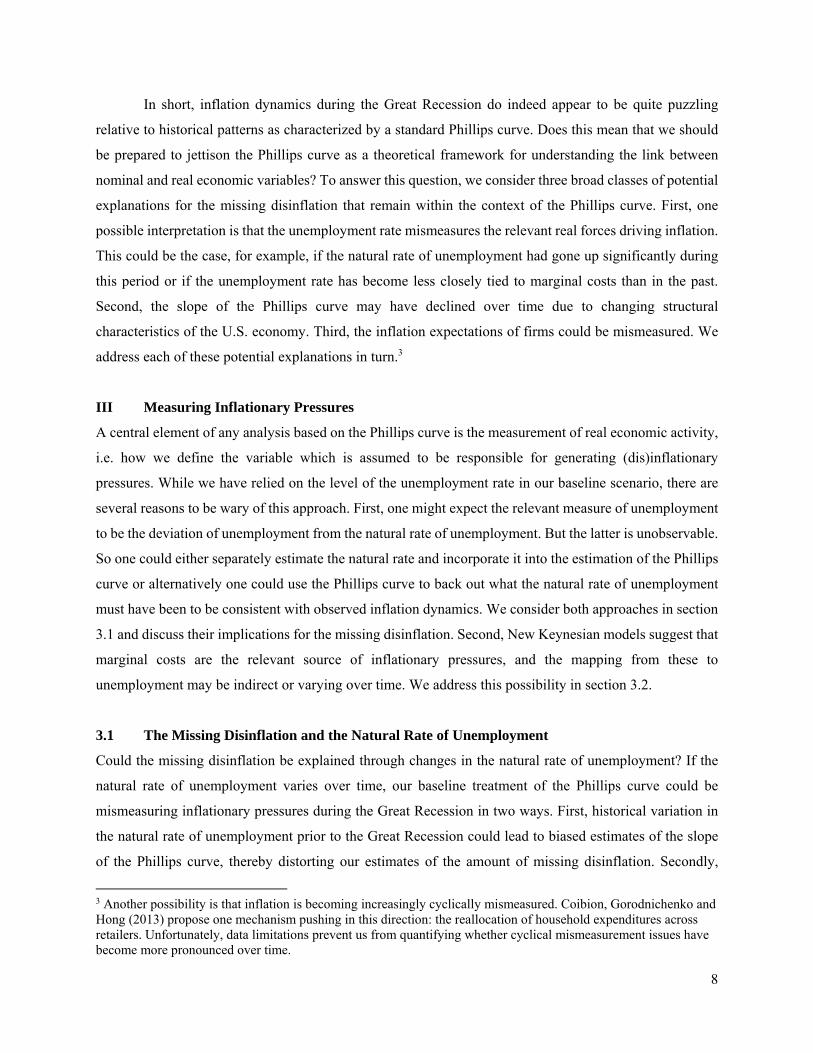
To address these possibilities, we first assume that the natural rate of unemployment is observable,
and use the estimate of the short-term natural rate of unemployment ( ) constructed by the
Congressional Budget Office (CBO). We then construct unemployment gaps as the quarterly deviation of
unemployment from the natural rate and treat this as the relevant forcing variable
in the Phillips curve
. (3)
CBO estimates of the natural rate of unemployment are available since 1949, so we can reproduce our
baseline Phillips curve relationship replacing unemployment rates with unemployment gaps. This is plotted
in Panel A of Figure 3. Focusing first on the pre-Great Recession period, we find that using the
unemployment gap has no material effect on the estimated slope—if anything the slope gets steeper—and
it improves the fit of the regression substantially, with the R2 rising to 0.15 from 0.13. But the absence of
any meaningful change in the estimated slope of the Phillips curve implies that pre-Great Recession
variation in the natural rate of unemployment does not have much effect on the degree of the missing
disinflation. Furthermore, because the CBO estimate of the natural rate of unemployment goes up only one
percentage point over the course of the Great Recession, inflation from 2009 to 2011 continues to stand out
as puzzlingly high relative to the rate of economic activity during this time period. Hence, incorporating
time variation in the natural rate of unemployment improves the historical fit of the Phillips curve but does
not meaningfully change the amount of missing disinflation.
How much would the natural rate of unemployment need to have changed during the Great
Recession to account for the missing disinflation? One can use the estimated Phillips curve to solve for the
evolution of the natural rate of unemployment needed to account for inflation dynamics (under the
assumption of no shocks to the Phillips curve over this time period). We implement this idea and plot the
resulting estimate of the natural rate of unemployment from 2007 on, along with 95% confidence intervals,
in Panel B of Figure 3.4 For comparison, we also plot the CBO estimate of the natural rate as well as the
actual level of unemployment over the corresponding period. The result is striking: to account for the
missing disinflation, the natural rate of unemployment would have needed to track actual unemployment
4 For this exercise only, we estimate the slope of the Phillips curve putting unemployment on the left hand side and inflation surprises on the right hand side. Using our original estimate of the slope of the Phillips curve yields even larger implied movements in the natural rate of unemployment.
10
very closely over the entire period of the Great Recession, implying that essentially all of the unemployment
dynamics during the Great Recession must have been structural.5
We interpret the dynamics of the natural rate of unemployment needed to account for the missing
disinflation as being too at odds with other empirical evidence to treat this as a plausible explanation. Elsy,
Hobijn, and Sahin (2010), Daly et al. (2012) and others use employment/unemployment flows to study
whether the natural rate of unemployment has changed since the start of the Great Recession and to what
extent mismatch contributes to persistent unemployment. In a nutshell, this literature points to a rise in the
natural rate of unemployment with an upper bound of 1-1.5%, broadly in line with the CBO estimates. As
illustrated in Panel A of Figure 3, this kind of variation in the natural rate of unemployment is too small to
change the conclusion that inflation was significantly higher between 2009 and 2011 than what would have
been expected from the previous historical experience.
3.2 Marginal Costs and the Missing Disinflation
An alternative explanation for the missing disinflation is that inflation is tied to marginal costs which have
behaved unusually during the recent period, thereby driving inflation dynamics. For example, New
Keynesian models a la Woodford (2003) or Clarida, Gali and Gertler (1999) yield expectations-augmented
Phillips curves in which marginal costs are the relevant forcing variables. While it is common in these
models to use labor’s share as a proxy for marginal costs (e.g. Gali and Gertler 1999), this measure has
become increasingly problematic over time. First, labor’s share of income has experienced a pronounced
decline since the 1980s (Karabarbounis and Neiman 2013). If one takes labor share as the appropriate
measure of marginal costs, this decline should have led to massive disinflationary pressures and, hence, the
magnitude of the missing disinflation would have been even more striking. However, King and Watson
(2012) document that recent movements in the labor share are largely due to low frequency variation which
makes using labor share (or unit labor cost) a poor proxy for the cyclical dynamics of marginal costs.
Second, there is likely to be significant mismeasurement of marginal costs because of the treatment of the
self-employed in the construction of labor’s share. Elsby, Hobjin and Sahin (2013) argue, for example, that
approximately one-third of the recent decline in labor’s share can be attributed to mismeasurement of the
wage income of the self-employed. They also argue that these measurement issues make labor’s share a
poor proxy for the cyclical variation in marginal costs.
To get around this issue, we focus primarily on the behavior of wages during the Great Recession
to ascertain whether marginal costs have behaved unusually during this period. Since the recent dynamics
of total factor productivity and labor productivity have been consistent with their behavior during other
5 This is not true by definition in an expectations-augmented Phillips curve, since changes in the unemployment gap affect the deviations of inflation from expected inflation, not just the level of inflation.
11
downturns (Fernald 2012), focusing on wages should be sufficient to isolate any unusual behavior in
marginal costs.
There are several mechanisms which could lead one to think that the missing disinflation can be
explained through unusual wage patterns. First, the share of the long-term unemployed has been unusually
high during the Great Recession relative to previous downturns (Coibion, Gorodnichenko and Koustas
2013). If the long-term unemployed have less pronounced effects on wage pressures than the short-term
unemployed (as suggested in Aaronson et al. 2010), then one could potentially explain the absence of
significant price disinflation through an absence of wage disinflation. A second mechanism is through
downward nominal wage rigidity. Falling levels of inflation since the early 1980s have also lowered average
nominal wage changes, so that an increasing share of workers appears to be experiencing zero wage changes
each year, i.e. wage adjustment is increasingly constrained by downward wage rigidity (Daly et al. 2012).
Again, this mechanism could explain the absence of price disinflation during the Great Recession through
an absence of wage disinflation.
Was the Great Recession also characterized by a missing wage disinflation, as suggested by both
of these mechanisms? Building on Coibion, Gorodnichenko and Koustas (2013), we address this question
by looking at wage Phillips curves of the same form as the price Phillips curve of section 2. Specifically,
we regress quarterly wage inflation net of expectations of wage growth on unemployment rates
(4)
using pre-Great Recession data to determine whether the experience during the Great Recession was
unusual. We first consider backward-looking specifications of expectations, assuming
. Because of the inherent difficulty of measuring wages, we consider
multiple measures of wage inflation. First is average hourly earnings of manufacturing workers. This
measure is narrow in its scope but likely reduces the measurement error associated with wages. Second is
compensation per hour in the non-farm business sector. In Panels A and B of Figure 4, we plot
unemployment against wage inflation net of expectations for each measure of wages respectively, along
with the implied slope of the wage Phillips curve during the pre-Great Recession period. We split this
sample into two (1960-1985 and 1986-2007) to assess whether the slopes are sensitive to the sample. In
each case, we find negative relationships between unemployment and wage inflation net of expectations
with no evidence of instability in these relationships over time. We then plot the corresponding values since
the start of the Great Recession. In each case, observations are distributed evenly around the predicted
values from the pre-Great Recession period. Thus, we find no evidence of a missing wage disinflation
during the Great Recession.
To assess whether this is robust to assumptions about expectations of wage inflation, we consider
a third measure of compensation: weekly manufacturing earnings. This measure is useful because real-time
12
forecasts of wage inflation are available for this series from the Livingston Survey of Forecasters. The latter
is a semi-annual survey in which forecasters were asked to predict the level of weekly manufacturing
earnings six months and twelve months ahead. From this survey, we can construct the expected wage
inflation over that six month period (i.e. at the semi-annual frequency). We present the resulting
semi-annual deviations of wage inflation from expected wage inflation against semi-annual unemployment
from 1960S1 to 2007S2 in Panel C of Figure 4. As with the two other measures of wage inflation, we find
that the slope of the wage Phillips curve appears to have been stable across the pre-Great Recession sample
and that wage outcomes during the Great Recession period are fully in line with what the earlier historical
experience would have led one to expect.
In short, using different measures of wages and either backward or forward looking expectations,
we find no evidence of missing wage disinflation during the Great Recession. This implies that one cannot
explain the missing price disinflation by appealing to mechanisms which rely on unusual wage dynamics
during the Great Recession, such as downward wage rigidity or differential wage pressures associated with
the long-term unemployed. Combined with the absence of unusual productivity dynamics documented in
Fernald (2012), these results imply that marginal costs are unlikely to have displayed unusual cyclical
dynamics during the Great Recession and therefore that the explanation for the missing disinflation does
not stem from unusually high costs but rather from the pricing decisions of firms conditional on typical
cyclical cost patterns.
IV The Slope of the Phillips Curve
A second class of explanations for the missing disinflation is that the slope of the Phillips curve has declined
over time, so that the historical relationship between the level of real economic activity and inflation may
be a misleading guide to recent inflation dynamics. In this section, we first investigate the extent to which
the slope of the Phillips curve may have changed, then turn to considering whether changes in the structure
of the U.S. economy can potentially explain time variation in the estimated slope of the Phillips curve, and
finally assess the quantitative importance of the declining slope of the Phillips curve in accounting for
missing disinflation.
4.1 Has the Slope of the Phillips Curve Changed?
In Panels A and B of Figure 5, we consider the average relationship between unemployment and deviations
of inflation from expectations for two separate sub-periods: 1960-1985 and 1986-2007, using backward
and forward looking expectations respectively. In each case, and consistent with Coibion, Gorodnichenko
and Koustas (2013), we can observe an apparent flattening of the slope of the Phillips curve. Hence, it
13
appears plausible that a flattening of the Phillips curve could potentially explain some of the missing
disinflation.
We investigate the statistical evidence for a change in the slope of the Phillips curve more formally
by allowing for a break in the slope of the Phillips curve in 1985Q1 as follows:
, , (5)
where , is a dummy variable equal to one for periods from 1985Q1 to 2007Q3 and zero prior to 1985.
The interaction of this dummy variable with the unemployment gap ( ) allows us to assess whether the
slope of the Phillips curve changed around this period.
We report results from estimating this specification in Table 1 for several cases: CPI inflation and
backward-looking expectations, GDP deflator inflation and backward-looking expectations, and GDP
deflator inflation with forward-looking (SPF) expectations.6 In each case, we estimate the Phillips curve
both by OLS as well as by IV, using as instruments a constant, one lag of unemployment, the dummy
variable for post-84 periods, and the interaction of the dummy with the lag of unemployment.
The point estimates on the interaction term are always positive, so that the Phillips curve
consistently appears to have flattened since the mid-1980s. However, the statistical significance of this
effect varies by specification: we cannot reject the null of no change in slope using the CPI but can reject
the null at least at the 5% level for all specifications with the GDP deflator, with almost no difference
between OLS and IV estimates in any case. Thus the evidence for a change in the slope is mixed. What is
consistent across specifications, however, is that the change in the slope (if there was one) was relatively
large: on the order of a 60-80% reduction in most specifications. Furthermore, we cannot reject the null that
the slope of the Phillips curve since 1985 was zero, pointing to a weak link between real and nominal
economic activity during this period, consistent with Atkeson and Ohanian (2001). The absence of
conclusive empirical evidence on a changing slope of the Phillips curve is problematic if this is the
underlying cause of the missing disinflation. So in the next section, we consider whether changes in the
structural parameters which determine the slope of the Phillips curve can potentially account for the
magnitudes of a change in slope needed to explain the missing disinflation.
4.2 Can Structural Changes Account for a Changing Slope of the Phillips Curve?
When the Phillips Curve is expressed in terms of employment, the slope of the New Keynesian Phillips
Curve (NKPC) in the basic model (e.g., Gali 2008; one input, perfectly mobile labor; capital is fixed and
normalized to be equal to one) is given by
6 We use GDP deflator inflation forecasts from the SPF because projections for the GNP/GDP deflator have been collected by the SPF since 1968 while CPI inflation projections have been collected by the SPF only since 1981. The short time series of the CPI projections in the SPF makes the analysis of structural breaks problematic.
14
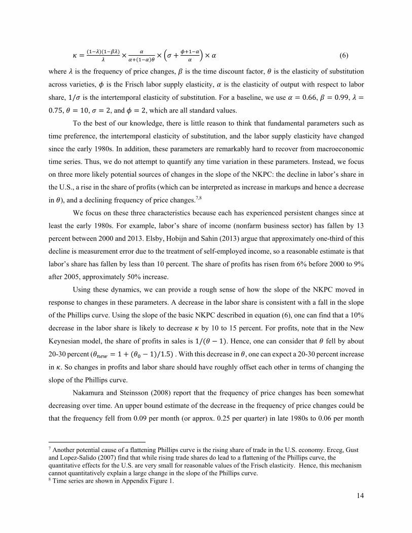
(6)
where is the frequency of price changes, is the time discount factor, is the elasticity of substitution
across varieties, is the Frisch labor supply elasticity, is the elasticity of output with respect to labor
share, 1/ is the intertemporal elasticity of substitution. For a baseline, we use 0.66, 0.99,
0.75, 10, 2, and 2, which are all standard values.
To the best of our knowledge, there is little reason to think that fundamental parameters such as
time preference, the intertemporal elasticity of substitution, and the labor supply elasticity have changed
since the early 1980s. In addition, these parameters are remarkably hard to recover from macroeconomic
time series. Thus, we do not attempt to quantify any time variation in these parameters. Instead, we focus
on three more likely potential sources of changes in the slope of the NKPC: the decline in labor’s share in
the U.S., a rise in the share of profits (which can be interpreted as increase in markups and hence a decrease
in ), and a declining frequency of price changes.7,8
We focus on these three characteristics because each has experienced persistent changes since at
least the early 1980s. For example, labor’s share of income (nonfarm business sector) has fallen by 13
percent between 2000 and 2013. Elsby, Hobijn and Sahin (2013) argue that approximately one-third of this
decline is measurement error due to the treatment of self-employed income, so a reasonable estimate is that
labor’s share has fallen by less than 10 percent. The share of profits has risen from 6% before 2000 to 9%
after 2005, approximately 50% increase.
Using these dynamics, we can provide a rough sense of how the slope of the NKPC moved in
response to changes in these parameters. A decrease in the labor share is consistent with a fall in the slope
of the Phillips curve. Using the slope of the basic NKPC described in equation (6), one can find that a 10%
decrease in the labor share is likely to decrease by 10 to 15 percent. For profits, note that in the New
Keynesian model, the share of profits in sales is 1/ 1 . Hence, one can consider that fell by about
20-30 percent ( 1 1 /1.5 . With this decrease in , one can expect a 20-30 percent increase
in . So changes in profits and labor share should have roughly offset each other in terms of changing the
slope of the Phillips curve.
Nakamura and Steinsson (2008) report that the frequency of price changes has been somewhat
decreasing over time. An upper bound estimate of the decrease in the frequency of price changes could be
that the frequency fell from 0.09 per month (or approx. 0.25 per quarter) in late 1980s to 0.06 per month
7 Another potential cause of a flattening Phillips curve is the rising share of trade in the U.S. economy. Erceg, Gust and Lopez-Salido (2007) find that while rising trade shares do lead to a flattening of the Phillips curve, the quantitative effects for the U.S. are very small for reasonable values of the Frisch elasticity. Hence, this mechanism cannot quantitatively explain a large change in the slope of the Phillips curve. 8 Time series are shown in Appendix Figure 1.
15
(or approx. 0.17 per quarter) in early 2000s. With this magnitude of a decrease, one can expect to fall by
as much as 50 percent. But other evidence such as Klenow and Kryvtsov (2008) documents almost no
variation in the frequency of price changes from 1988 to 2004, so the contribution of a changing frequency
of price setting is unlikely to be anywhere near this large. Thus, a declining frequency of price changes may
have led to some flattening of the Phillips curve, but it is very unlikely to generate the kind of flattening
suggested by the estimates of Table 1.
Another possible source of a flattening Phillips curve is the decline in trend inflation since the highs
of the 1970s. While our baseline Phillips curve follows from New Keynesian models log-linearized around
zero trend inflation, incorporating positive levels of inflation yields a more complex expression for inflation
dynamics in which inflation becomes increasingly forward-looking at higher levels of steady-state inflation
(Ascari and Ropele 2007, Coibion and Gorodnichenko 2010). Thus, the decline in inflation since the 1970s
could have led to a flatter reduced-form Phillips curve relationship between inflation surprises and real
activity through this alternative channel. To quantify this possibility, we simulate the calibrated New
Keynesian model of Coibion, Gorodnichenko and Wieland (2012) at different steady state levels of inflation
and evaluate the extent to which changes in steady-state inflation affect the slope of the reduced form
Phillips curve. We find that plausible reductions in steady-state inflation (e.g. from 6% to 2% per year)
have very little effect on the slope of this relationship, accounting for less than a 10% decline. Thus, this
mechanism also cannot account for the magnitude of the decline in the Phillips curve suggested in Table 1.
4.3 Can a Changing Slope of the Phillips Curve Account for the Missing Disinflation?
The empirical evidence on whether the slope of the Phillips curve has changed is mixed, with some
estimates of the Phillips curve rejecting stability while others not. Furthermore, we cannot identify any clear
economic mechanism to explain the magnitude of empirical estimates of the change in the slope of the
Phillips curve. We now consider whether, if we take the estimates of the change in slope at face value, the
declining slope can account for the missing disinflation.
Specifically, we produce counterfactual time paths of inflation during the Great Recession based
on both the full-sample estimates of the Phillips curve as well as the restricted sample estimates from the
more recent period. We do so for CPI inflation using either backward-looking or SPF expectations. The
results are presented in Panel C of Figure 5. We find modest effects from changes in the slope. With
backward-looking expectations, the average inflation rate over the sample is higher by approximately 1%,
but this leaves most of the missing disinflation unexplained. With SPF expectations, the change in slope
raises average inflation during the Great Recession by approximately 0.5%, again leaving much of the
missing disinflation unexplained. In short, even if we accept the possibility of a change in slope (which is
16
statistically tenuous and unexplained by economic fundamentals), this explanation can quantitatively
account for only a fraction of the missing disinflation.
V Inflation Expectations
After the level of real economic activity and the slope of the Phillips curve, the third source of a potential
explanation for the missing disinflation within the context of the Phillips curve is through the behavior of
firms’ inflation expectations. A key limitation of inflation expectations data is that there is no survey
focused explicitly on the beliefs of firms. While reliable data exist on the inflation forecasts of households
(U. of Michigan Survey of Consumers), professional forecasters (Survey of Professional Forecasters,
Livingston Survey), and central bankers (Greenbook forecasts), there is no comparable data for firms whose
price-setting decisions determine inflation dynamics in the economy. Despite this, we show in this section
that the most likely source of the missing disinflation lies precisely in the inflation expectations of firms.
5.1 Alternative Measures of Inflation Expectations and the Missing Disinflation
The absence of inflation forecasts on the part of firms could be a severe constraint if their expectations
differ significantly from those of other agents. Is there any evidence of important differences in beliefs
across agents in the economy for whom we have data? Panel A of Figure 6 plots the time series of mean
inflation forecasts for professional forecasters (SPF forecasts of year-ahead annual CPI inflation) and those
of households (U. of Michigan Survey of Consumers forecast of price changes over the next 12 months)
since 1980. In addition, we plot inflation forecasts extracted from asset prices as a measure of the beliefs
of financial market participants.9 While forecasts from asset prices have tracked those of professional
forecasters closely over most periods, households have reported inflation forecasts which have differed
noticeably from those of professionals and financial market participants on a number of occasions. For
example, households reported higher inflation forecasts for much of the mid-1990s, in 2000, and
systematically so since 2003. But the forecasts of households appear to differ by more than just a fixed
amount: we can also observe quite different dynamics on a number of instances. For example, households
reported a much larger increase in inflation forecasts in 2008 than did professional forecasters and also
reported much larger declines immediately thereafter. More importantly, whereas professional forecasters
and financial market participants have reported near-constant year ahead inflation forecasts since 2009,
households have been reporting rising inflation forecasts over the same period, with the mean forecast rising
from 2.5% in 2009 to a peak of 5% in 2011 and remaining in the range of 4% after 2011.
9 The series of inflation expectations from asset prices is produced by the Federal Reserve Bank of Cleveland. The method for the constructing these expectations is described in Haubrich et al. (2008).
17
Because we do not directly observe firms’ inflation forecasts, these differences in inflation
expectations between households and professional forecasters suggest that one should be wary of assuming
that the expectations of firms are necessarily well-proxied by professional forecasts. One might expect, for
example, very large firms to have professional forecasters on staff or to rely on the services of professional
forecasters to guide their economic decisions. But this need not be the case for small and medium enterprises
for whom the gains from having precise information about aggregate conditions may be small (especially
relative to local or industry-specific conditions), as in Mackowiak and Wiederholt (2009). For such firms,
household forecasts could very well be a better proxy of their beliefs than professional forecasts.
Does it matter for the Phillips curve and the missing disinflation whether one assumes that firms
hold beliefs closer to those of professional forecasters or households? We showed in Panel E of Figure 1
that using professional forecasts of inflation did not meaningfully affect the estimated slope of the historical
Phillips curve or the presence of missing disinflation during the Great Recession. In Panel B of Figure 6,
we present the Phillips curve relationship between the unemployment gap and the difference between CPI
inflation and household expectations of inflation. Several facts stand out. First, in the pre-Great Recession
period, the relationship between unemployment gaps is systematically negative, and unlike the evidence
with SPF forecasts, there is no evidence of a decline in the slope of the Phillips curve over time. Second,
the Phillips curve is flatter than that found with SPF forecasts or backward-looking expectations but
significantly different from zero. Third, there is no evidence of missing disinflation during the Great
Recession once one conditions on household forecasts: this reflects both a flatter Phillips curve in the pre-
Great Recession period and higher levels of inflation expectations between 2009 and 2011 than when using
either professional or backward-looking forecasts. Panel C in Figure 6 plots the predicted time series of
inflation during the Great Recession period (given actual unemployment gaps and actual expectations)
using SPF forecasts, backward-looking expectations and household expectations. While using either
backward or professional forecasts yields predictions of inflation that are much lower than actually
experienced between 2009 and 2011, using household inflation forecasts eliminates this and yields a
prediction of inflation that averages around 2-3% over this period. Thus, if the forecasts of price-setting
firms have been more in line historically with those of households than professional forecasters, then one
could fully explain the missing disinflation through their inflation expectations.
Is the ability of household inflation expectations to resolve the missing disinflation occurring
because of the flatter estimated slope in pre-Great Recession periods or by the behavior of household
expectations during the Great Recession? In Panel D of Figure 6, we present two additional counterfactuals
paths of inflation to distinguish between these two possibilities. First, we use the SPF inflation expectations
combined with the estimated slope of the Phillips curve from household expectations: we find that the
predicted level of inflation is almost identical to that of SPF inflation expectations with SPF estimate of the
18
slope of the Phillips curve. Thus, the slightly smaller estimated slope of the Phillips curve found using the
household expectations has almost no effect on predicted inflation. Second, we use the household inflation
expectations combined with the estimated slope of the Phillips curve from SPF expectations: we find that
the predicted level of inflation is very close to that of household expectations combined with household
estimate of the slope of the Phillips curve. Thus, it is the specific behavior of household inflation
expectations during and since the Great Recession which can account for the missing disinflation.
5.2 Are Firms’ Inflation Forecasts Well Represented by Household Inflation Forecasts?
The evidence presented above that the missing disinflation can be explained through household forecasts
is, of course, only suggestive. How can we discern whether firms’ inflation forecasts tend to be better
proxied by household forecasts than professional forecasts? One possibility is to use the Phillips curve itself
to answer this question, since the link between inflation and real economic activity stems from the pricing
decisions of firms and their beliefs about future macroeconomic outcomes. Specifically, we can estimate a
nested Phillips curve
(7)
which includes forecasts of both households and professional forecasters along with the unemployment
gap. If firms’ forecasts are better proxied by household forecasts when they set prices, then one would
expect to find 1, 0 while the null that their forecasts are better proxied by professional forecasts
is that 0, 1.
Because the measure of inflation which likely corresponds most closely to household inflation
forecasts is the CPI, we focus on the period since 1981 for which SPF forecasts of CPI inflation are
available. We use SPF forecasts of inflation over the next four quarters ( ,
for comparison with household forecasts which are specified over the next 12 months.
We estimate several versions of this specification: including and excluding the Great Recession, using the
unemployment rate ( ) or the unemployment gap ( ), unrestricted and restricted
coefficients on forecasts ( 1), and controlling for contemporaneous oil price changes or not.
The results are presented in Table 2 and are largely insensitive to the empirical specification. The
key finding is that across specifications, household forecasts receive a weight of around 1 which is
significantly different from zero whereas professional forecasts receive a weight of close to 0, for which
we can generally not reject the null of zero coefficient. Thus, household forecasts appear to be a more
relevant measure of inflation forecasts for the Phillips curve than professional forecasts. In Appendix Table
1, we document that household inflation forecasts similarly dominate backward-looking forecasts. Since
the underlying mechanism for the Phillips curve reflects firms’ expectations of future aggregate outcomes,
19
these results suggest that it is indeed reasonable to treat firms’ forecasts as more closely approximated by
household forecasts than those of professional forecasters.
A second approach to assessing whether firms’ beliefs are better approximated by household
forecasts or professional forecasts is via quantitative surveys of firms’ expectations. While no such data
exists for the U.S., in ongoing work (Coibion, Gorodnichenko and Kumar 2014) we are conducting a survey
of firms in New Zealand which includes questions about their inflation expectations. While the survey will
take some time to complete, we first did a trial run of the survey questions in September 2013 on sixty
randomly drawn firms (twenty manufacturing, twenty retail firms, and twenty financial and business service
firms) from which we can draw some preliminary inference about the properties of firms’ inflation
expectations. Each of these firms was contacted by phone and the general manager provided detailed
responses to a number of questions. One such question was “During the next twelve months, by how much
do you think prices will change overall in the economy? Please provide a quantitative answer.” This
question is almost identical to that asked of households in household surveys of inflation expectations and
therefore allows us to compare moments of household and firm forecasts at one point in time.
We present some summary statistics about firms’ answers to these questions in Table 3, along with
comparable forecasts from households, professional forecasters, and the central bank of New Zealand, all
from September 2013. The survey of households is run by the Reserve Bank of New Zealand and is a
monthly survey which asks approximately 1,000 households about their expectations of inflation over the
next twelve months.10 Professional forecasts are from Consensus Economics and covers fifteen professional
forecasters of the New Zealand economy. Because these forecasts are for calendar years, we impute
individual 12-month ahead forecasts as / / . The Reserve Bank of New
Zealand also provides forecasts of annual CPI inflation in its Monetary Reports, so we include its forecast
of annual CPI inflation for September 2014 from the September 2013 report.
While annual CPI inflation in New Zealand in September 2013 was running at only 0.7%, the
Reserve Bank was forecasting a rise in prices of 1.7% over the next twelve months. Professional forecasters
were anticipating a similar rise of 1.9%. The standard deviation of inflation forecasts across professional
forecasters was very low at 0.2%, with the lowest forecast being 1.5% and the highest being 2.1%. In
contrast, households were expecting a much higher level of inflation over the same period, with the mean
forecast across all households being 5.3%. The Reserve Bank of New Zealand presents a truncated version
of household expectations in its Monetary Report, dropping all forecasts of inflation which are less than or
equal to -2% or greater than or equal to 15%. The mean forecast across this subset of households was 3.1%,
still well above that of professionals or the central bank. More strikingly, the cross-sectional dispersion of
10 We are grateful to Graham Howard from the Reserve Bank of New Zealand for providing detailed statistics from the September 2013 survey of households.
20
forecasts across households was much larger than that of professionals, with a cross-sectional standard
deviation of 5.3% for all households and 1.7% for the truncated set of households.
The large dispersion of household forecasts relative to professionals is a typical characteristic. We
produce equivalent statistics for the U.S., using the February 2013 Michigan Survey of Consumers for
households (the most recent date for which underlying microdata are available at the time of writing this
paper), professional forecasts of U.S. CPI inflation from the February 2013 Consensus Economics and the
FOMC midpoint forecast of PCE inflation from the March 2013 projections. Both the professional and
central bank forecasts are very close to those of New Zealand, but again the household forecasts have both
a higher mean and much higher dispersion of forecasts, on the same order as that observed for households
in New Zealand.
How do firms’ forecasts compare to professionals and households in New Zealand? We provide
summary statistics for year-ahead forecasts of all firms, all firms with the same truncation as used by the
Reserve Bank of New Zealand, the subset of 40 non-financial firms and this subset truncated in the same
way. Note that the truncation of forecasts eliminates only one manufacturing firm and no retail firms, but
removes eleven out of twenty financial and business service firms. The firms in the sample vary
significantly by age (average age of 23 years with minimum of 3 years and maximum of 155 years) and
size (the number of full-time employees is 23 on average, with a minimum of 7 and a maximum of 85).
Like households, average inflation forecasts for firms were much higher than those of professional
forecasters, with median forecasts around 5%. More strikingly, the dispersion of forecasts is of the same
order of magnitude as that of households and much larger than anything observed among professional
forecasters. Thus, at least along this key dimension which differentiates household and professional
forecasts, the evidence suggests that inflation forecasts of firms are much more similar to those of
households than those of professional forecasters.
5.3 Why Have Household Inflation Forecasts Evolved Differently in Recent Years?
The results in the previous sections document that one can fully explain the missing disinflation if firms
held approximately the same expectations as households, and that this is likely to be a reasonable
description in practice. But why did households hold such different beliefs than professional forecasters?
Our suggested answer can be seen in Panel A of Figure 7. Household inflation forecasts have tracked the
price of oil extremely closely since the early 2000s, with almost all of the short-run volatility in inflation
forecasts corresponding to short-run changes in the level of oil prices. From January 2000 to March 2013,
for example, the correlation between the two series was 0.74. In contrast, the correlation between SPF
inflation forecast and oil price over the same period was -0.12. The strong sensitivity of consumers’ inflation
21
expectations to oil price has historically been strong: the correlation between MSC inflation expectations
and real oil price over 1960-2000 was 0.67.
To assess the link between household inflation expectations and commodity prices more formally,
we regress the difference between households’ mean inflation forecast and that of professional forecasters
on measures of commodity prices, both in levels and first-differences. For consistency in forecasts, we
focus on SPF forecasts of the CPI, which are available since 1981. The results are presented in Table 5.
First, we find that the level of the oil price (West Texas Intermediate) is a statistically significant predictor
of the difference in inflation forecasts, with higher oil prices being associated with higher inflation forecasts
by households relative to professional forecasters. Furthermore, the quantitative power of oil prices in
accounting for this differential is very large, with the R2 being slightly over 50%. In contrast, while the
change in oil prices is a statistically significant predictor of the difference in inflation forecasts across
households and professionals, its quantitative importance is limited, with an R2 of less than 5%. Thus, it is
primarily the level, rather than the change, of oil prices that drives differences in the inflation forecasts of
households and professionals.11
We can also verify whether the rise in oil prices can quantitatively account for the increase in
household expectations of inflation relative to professional forecasts since 2009. The price of West Texas
Intermediate went from under $40 per barrel in February of 2009 to over $100 per barrel in early 2012.
This sixty dollar rise in the price of oil would have been predicted to raise household inflation forecasts by
approximately 1.6 percentage points relative to SPF forecasts. Since household forecasts rose from a low
of around 2.5% in early 2009 to 4% since 2011 while professional forecasts remained close to 2%, the rise
in oil prices can account for all of the rise in household inflation expectations relative to those of
professional forecasters over this time period.
This high sensitivity of household inflation forecasts to oil prices relative to that of professional
forecasters should not necessarily be interpreted as reflecting “excess sensitivity” on the part of households.
Coibion and Gorodnichenko (2012) document that both professional and household inflation forecasts tend
to under-respond to oil price shocks relative to the actual response of inflation, but that the forecast errors
of households after oil price shocks dissipate more quickly than those of professionals. The results in Table
5 therefore confirm that household forecasts respond more rapidly to oil price movements than professional
forecasters.
While it may seem surprising for households to adjust their forecasts more rapidly than professional
forecasters, gasoline prices are among the most visible prices for most individuals and they likely play a
11 We found similar qualitative results going back to 1968 by comparing household inflation forecasts with the SPF forecast of the GDP deflator. However, these are harder to interpret because the effects of oil price changes on the CPI and the GDP deflator could themselves be different.
22
predominant role in affecting people’s perceptions of broader price movements. Indeed, in Table 5, we also
find that household inflation forecasts respond more strongly than professional forecasts to food prices, as
measured by the World Bank’s food commodity price index, with levels again accounting for much larger
fraction of the variance in inflation forecast differentials between households and professionals than first-
differences. This is consistent with the idea that households pay attention to the prices which they observe
frequently, although regressions including both oil and food prices suggest that oil prices play the
predominant role in accounting for the deviation of household inflation forecasts from those of
professionals.
To investigate this hypothesis further, we exploit the micro-data of the Michigan Survey of
Consumers. Specifically, we use the panel structure of the data and study the revisions in individual inflation
forecasts across 6-month periods (two thirds of new households in each month’s survey are interviewed
again six months later), thereby controlling for individual fixed effects. We then regress individual changes
in inflation forecasts against the change in oil prices over the same time period, i.e.
, , log 100 , (7)
where i and t index individuals and time, , is one-year-ahead inflation expectations of individual i
at time t, is the price of oil (West Texas Intermediate) at time t. Another advantage of focusing on oil
prices is that gasoline, unlike e.g. food or clothing, is a homogenous commodity and hence consumers do
not need to wrestle with issues related to changes in quality vs. changes in prices.
The first row of Table 6 documents that, across all households, higher oil prices are associated with
higher inflation forecasts on the part of individuals: households revise their inflation expectations by 1.6
percent in response to a one percent increase in oil prices. This is a remarkably high sensitivity given that
spending on gas and fuel has a relatively small share in total spending for typical households.
In general, one could expect cross-sectional differences in individual responses to oil price changes
to reflect (at least) two sources. First, as suggested before, individuals may use highly visible oil/gas prices
as a signal of other price changes. One would expect this effect to be stronger for households who purchase
gasoline more often. Alternatively, households may not be reporting forecasts of overall inflation of the
economy when they respond to surveys but rather expected changes in the price of their own consumption
bundles. One would then expect households who spend a large share of their income on gasoline to adjust
their inflation forecasts more in response to oil price changes.
With individual data on forecast revisions, we can distinguish between these two possibilities. The
Bureau of Labor Statistics (BLS 2013), for example, reports that higher income people on average spend
more money on gasoline than lower income people (and therefore purchase gasoline more frequently) but
spend a much smaller share of their income on gasoline than lower income groups. The top quintile, for
23
example, spent more than three times as much as the bottom quintile on gasoline in 2011 ($4,073 vs. $1,227
per year), but this was a smaller share of their expenditures than for the bottom quintile (4.3% vs. 5.6%). If
the effect of oil price changes on inflation forecasts reflects the effect on the forecasted price of the
individual’s consumption bundle, then we would expect to see lower income households adjust their
inflation forecasts by more than higher income households. But if it instead reflects how frequently an
individual observes gasoline prices, one would expect the high income household to adjust their inflation
forecast by more. Hence, decomposing the sensitivity of inflation forecast changes to oil price changes by
subgroups can help identify the source of households’ high sensitivity to oil prices, which appears to have
played such a prominent role in explaining the missing disinflation. To this end, we also estimate two
additional regressions:
, , log 100 log , (8’)
, , log 100 log$
$ , (8’’)
where is the share of spending on gasoline for individual i and $ is the dollar amount of
spending on gasoline for individual i, and $ are the budget share and dollar spending on
gasoline for a baseline group (e.g., the bottom income quintile or age group 18-24). In the Michigan Survey
of Consumers we do not observe spending patterns of individual households but we do know if a given
household (or household head) belongs to a given income quintile or age group. Using statistics from the
Consumer Expenditure Survey, we can assign spending and budget shares to households based on the age
or income they report in the Michigan Survey of Consumers. While this approach is likely to introduce
errors in how a given household spends its resources, it provides crucial cross-sectional variation in the
survey data that can be used to validate time-series results.
In Table 6, we present estimates of equation (7) across households by income quintile. We find that
the coefficient on oil price changes is strictly increasing in income: higher income households adjust their
inflation forecasts by more than low income households when oil prices change. Given that high income
households spend more on gasoline in dollar terms but a smaller fraction of their income, this supports the
idea that the sensitivity of household inflation forecasts to oil prices reflects the visibility of gasoline prices.
We also consider estimates of equations (8’) and (8’’) across all households but interacting income quintiles
with the change in oil prices: this confirms that higher quintiles are on average more sensitive to oil price
changes. Interactions with budget shares instead point in the opposite direction.
We consider a similar decomposition by age group. While gasoline expenditures are falling as a
share of income with age, gasoline expenditures in dollar terms are highest for middle-aged individuals (35-
54). Consistent with the notion that it is more frequent exposure to gasoline prices that affects individual
24
sensitivity of inflation forecast revisions to oil price changes, we find that the coefficients on oil price
changes are highest for middle-aged individuals and lowest for young adults and seniors. Thus, there is a
clear positive relationship between the effect of oil price changes on inflation forecast revisions and dollar
expenditures on gasoline (and therefore the frequency of visits to gasoline stations) whereas there is no link
between this elasticity and expenditure shares of gasoline.12
5.4 Summary and Discussion
The use of household inflation forecasts as the measure of expectations in the Phillips curve can account
for the missing disinflation. The primary reason is that household inflation expectations went up sharply
between 2009 and 2011, thereby potentially preventing a downward adjustment of prices. We argued that
household expectations are likely to be a better proxy for firms’ inflation expectations than professional
forecasts, thereby justifying their inclusion in the Phillips curve. Our evidence is two-fold. First, in Phillips
curve regressions, household inflation forecasts are strictly preferred to either professional forecasts or
backward-looking expectations. Second, cross-sectional characteristics of a survey of firms’ expectations
in New Zealand support the notion that firm forecasts are more akin to those of households than professional
forecasts. We also provide a justification for why household expectations behaved so differently than
professional forecasters’ during the Great Recession: households are much more sensitive to oil price
changes when forming inflation forecasts than professional forecasters, and the magnitude of the run-up in
oil prices between 2009 and 2011 can fully account for the differential behavior of the expectations between
these agents.
Our explanation of the missing disinflation has some unusual implications. One is that advanced
economies may well have gotten lucky in the midst of the Great Recession: the surge in oil and commodity
prices between 2009 and 2011, driven largely by a resurgence of growth in developing economies (Kilian
and Murphy 2012, Alquist and Coibion 2013), boosted inflation expectations at just the right time. While
commodity price increases during this period likely had some negative consequences for employment,
preventing deflation via higher inflation expectations may well have avoided deflationary spiral
mechanisms which, in New Keynesian models, account for the large welfare costs of zero bound episodes
(Christiano, Eichenbaum and Rebelo 2011).
A second unusual implication is that a necessary condition for the oil price increases between 2009
and 2011 to have raised household (and firm) inflation expectations was that household expectations were
12 We explored additional dimensions available in the Michigan Survey of Consumers. For example, we found similar results as with income when we split the sample based on the educational attainment of household heads. That is, it is the dollar amount of spending rather than the budget share that determines households’ sensitivity to changes in oil prices. We also found that households with more cars (this information is available for the 1981-2003 period) are more sensitive to changes in oil prices.
25
not fully anchored. So whereas Bernanke (2010) suggested the anchoring of expectations as a possible
explanation for the absence of more disinflation during the Great Recession, our interpretation points
precisely in the opposite direction: had household expectations been more anchored like those of
professional forecasters, then disinflationary pressures would likely have been significantly more severe.
While anchored expectations may still be a desirable outcome for policymakers, our results point to at least
one experience in which this was not the case. This experience may prove to be particularly relevant as
policymakers increasingly resort to forward guidance in an attempt to affect agents’ economic expectations.
VI Conclusion
The absence of significant disinflation during the Great Recession has been a key puzzle for (New)
Keynesian models. A Phillips curve representation of the link between nominal and real activity suggests
that the severity of the economic downturn should have led to very low inflation or even deflation. The
absence of this disinflation has been advocated as evidence for a sizable increase in structural
unemployment or as evidence that (New) Keynesian models could not be reconciled with the experience of
the Great Recession, casting their usefulness as macroeconomic models into severe doubt.
While a number of potential explanations have been suggested, such as the “anchoring” of
expectations, downward wage rigidity, or a flattening of the Phillips curve, we find that none of these is a
satisfactory explanation. Instead, we propose a new explanation based on the idea that firms’ inflation
expectations are best proxied by household expectations and that an expectations-augmented Phillips curve
using household forecasts does not display any missing disinflation. Instead, the rise in inflationary
expectations between 2009 and 2011—which can be ultimately explained by the large increase in oil prices
of this period—can account for why inflation did not fall as much as one might have predicted.
We provide novel evidence for the key assumption underlying this explanation, namely that firm
expectations are best proxied by household expectations, both from regressions of the Phillips curve as well
as through direct survey evidence of firms’ inflation forecasts. But a productive avenue for future research
would be to delve more deeply into the key question of how firms form their expectations. Unfortunately,
there are no readily available quantitative survey data for firms’ expectations, so addressing this question
will be challenging. One approach is to consider in more detail the information problems faced by firms to
infer from theory how they might be choosing to acquire and process new information, for example as in
Reis (2006) or Mackowiak and Wiederholt (2012). An alternative is to develop new survey data of firms’
expectations to directly quantify the key properties of their expectations formation process, as we are doing
in ongoing work (Coibion, Gorodnichenko and Kumar 2014). Regardless of the methodology employed,
successfully characterizing how firms form their expectations strikes us as central to understanding more
deeply the link between the nominal and real sides of the economy. But in the meantime, our results suggest

26
that the Phillips curve remains one of the most useful conceptual frameworks for understanding the
relationship between prices and macroeconomic conditions.
27
References
Aaronson, Daniel, Bhashkar Mazumder, and Shani Schechter, 2010. “What is behind the rise in long-term unemployment?” Economic Perspectives, Federal Reserve Bank of Chicago, issue Q II, 28-51.
Akerlof, George A., William R. Dickens, and George L. Perry, 1996. "The Macroeconomics of Low Inflation," Brookings Papers on Economic Activity 27(1), 1-76.
Alquist, Ronald, and Olivier Coibion, 2013. “The Comovement of Commodity Prices: Sources and Implications,” manuscript.
Ascari, Guido, and Tiziano Ropele, 2007. “Optimal Monetary Policy under Low Trend Inflation,” Journal of Monetary Economics 54(8): 2568–2583.
Atkeson, Andrew, and Lee E. Ohanian., 2001. “Are Phillips curves useful for forecasting inflation?” Quarterly Review, Federal Reserve Bank of Minneapolis, issue Win, pages 2-11.
Ball, Laurence, and Sandeep Mazumder, 2011. “Inflation Dynamics and the Great Recession,” Brookings Papers on Economic Activity 42(1), 337-405.
Bernanke, Ben, 2010. “The Economic Outlook and Monetary Policy,” speech delivered at the Federal Reserve Bank of Kansas City Economic Symposium, Jackson Hole, Wyoming, August 27, 2010.
Bureau of Labor Statistics (BLS), 2013. “Consumer Expenditures in 2011” Report 1042, April 2013. Calvo, Guillermo A., 1983. “Staggered prices in a utility-maximizing framework,” Journal of Monetary
Economics, 12(3), pages 383-398. Christiano, Lawrence, Martin Eichenbaum, and Charles L. Evans, 2005. “Nominal Rigidities and the
Dynamic Effects of a Shock to Monetary Policy,” Journal of Political Economy, 113(1), 1-45. Christiano, Lawrence, Martin Eichenbaum, and Sergio Rebelo, 2011. “When Is the Government Spending
Multiplier Large?” Journal of Political Economy 119(1), 78-121. Coibion, Olivier, Yuriy Gorodnichenko, and Johannes Wieland, 2012. “The Optimal Inflation Rate in New
Keynesian Models: Should Central Banks Raise Their Inflation Targets in Light of the Zero Lower Bound?” Review of Economic Studies 79(4), 1371-1406.
Coibion, Olivier, and Yuriy Gorodnichenko, 2011. “Monetary Policy, Trend Inflation, and the Great Moderation: An Alternative Interpretation,” American Economic Review 101(1), 341-370.
Coibion, Olivier, and Yuriy Gorodnichenko, 2012. “What Can Survey Forecasts Tell Us about Information Rigidities?” Journal of Political Economy 120(1), 116 - 159.
Coibion, Olivier, Yuriy Gorodnichenko, and Dmitri Koustas, 2013. “Amerisclerosis? The Puzzle of Rising U.S. Unemployment Persistence,” forthcoming in Brookings Papers on Economic Activity.
Coibion, Olivier, Yuriy Gorodnichenko, and Gee Hee Hong, 2012. “The Cyclicality of Sales, Regular, and Effective Prices: Business Cycle and Policy Implications,” NBER WP w18273.
Coibion, Olivier, Yuriy Gorodnichenko, and Saten Kumar, 2014. “The Macroeconomic Expectations of Firms: New Evidence from a Quantitative Survey,” work in progress.
Daly, Mary C., Bart Hobijn, Ayşegül Şahin, and Robert G. Valletta. 2012. “A Search and Matching Approach to Labor Markets: Did the Natural Rate of Unemployment Rise?” Journal of Economic Perspectives 26(3): 3-26.
Daly, Mary, Bart Hobijn, and Brian Lucking, 2012. “Why Has Wage Growth Stayed Strong?” FRBSF Economic Letter 2012-10, April 2, 2012.
Dotsey, Michael, Robert G. King, Alexander L. Wolman, 1999. “State-Dependent Pricing and the General Equilibrium Dynamics of Money and Output,” Quarterly Journal of Economics 114(2), 655-690.
Elsby, Michael, Bart Hobijn, and Aysegul Sahin, 2013. “The Decline of the U.S. Labor Share,” forthcoming in Brookings Papers on Economic Activity.
Elsby, Michael, Bart Hobijn, and Ayşegül Şahin. 2010. “The Labor Market in the Great Recession.” Brookings Papers on Economic Activity (Spring): 1–48.
Erceg, Christopher, Christopher Gust, and David López-Salido, 2007. “The Transmission of Domestic Shocks in Open Economies,” in International Dimensions of Monetary Policy, pages 89-148, National Bureau of Economic Research, Inc.
28
Fernald, John, 2012. “Productivity and potential output before, during, and after the Great Recession,” Working Paper Series 2012-18, Federal Reserve Bank of San Francisco.
Friedman, Milton, 1968. “The Role of Monetary Policy,” American Economic Review 58, 1–17. Gali, Jordi and Mark Gertler, 1999. “Inflation Dynamics: A Structural Econometric Analysis,” Journal of
Monetary Economics 44(2), 195-222. Gali, Jordi, 2008. Monetary Policy, Inflation and the Business Cycle: An Introduction to the New Keynesian
Framework, Princeton University Press. Gertler, Mark, Jordi Gali, and Richard Clarida, 1999. “The Science of Monetary Policy: A New Keynesian
Perspective,” Journal of Economic Literature 37(4), 1661-1707. Gorodnichenko, Yuriy, 2008. “Endogenous Information, Menu Costs, and Inflation Persistence,” NBER
WP 14184. Haubrich, J., G. Pennacchi, and P. Ritchken, 2008. “Estimating Real and Nominal Term Structures using
Treasury Yields, Inflation, Inflation Forecasts and Inflation Swap Rates,” FRB Cleveland WP 08-10.
International Monetary Fund (IMF), 2013. “The Dog That Didn’t Bark: Has Inflation Been Muzzled or Was It Just Sleeping,” Chapter 3 in World Economic Outlook, April 2013.
Karabarbounis, Loukas, and Brent Neiman, 2013. “The Global Decline of the Labor Share,” NBER Working Paper 19136.
Kilian, Lutz, and Daniel P. Murphy, 2012. “Why Agnostic Sign Restrictions Are Not Enough: Understanding The Dynamics Of Oil Market VAR Models,” Journal of the European Economic Association 10(5), 1166-1188.
King, Robert G., and Mark W. Watson, 2012. “Inflation and Unit Labor Cost,” Journal of Money, Credit and Banking 44, 111-149.
Klenow, Peter J., and Oleksiy Kryvtsov, 2008. “State-Dependent or Time-Dependent Pricing: Does It Matter for Recent U.S. Inflation?” Quarterly Journal of Economics 123(3), 863-904.
Llaudes, Ricardo, 2005. “The Phillips Curve and Long Term Unemployment,” ECB Working Paper 441. Mackowiak, Bartosz, and Mirko Wiederholt, 2009. “Optimal Sticky Prices under Rational Inattention,”
American Economic Review 99(3), 769-803. Mackowiak, Bartosz, and Mirko Wiederholt, 2012, “Business Cycle Dynamics under Rational Inattention,”
manuscript. Mankiw, N. Gregory and Ricardo Reis. “Sticky Information Versus Sticky Prices: A Proposal To Replace
The New Keynesian Phillips Curve,” Quarterly Journal of Economics, 117(4), 1295-1328. Nakamura, Emi, and Jón Steinsson, 2008. “Five Facts About Prices: A Reevaluation of Menu Cost
Models,” Quarterly Journal of Economics 123(4), 1415-1464. Reis, Ricardo, 2006. “Inattentive Producers,” Review of Economic Studies, 73 (3), 793-821. Roberts, John M., 1997. “Is Inflation Sticky?” Journal of Monetary Economics, 39(2), 173-196. Taylor, John B, 1980. “Aggregate Dynamics and Staggered Contracts,” Journal of Political Economy,
88(1), pages 1-23. Woodford, Michael, 2003. Interest and Prices: Foundations of a Theory of Monetary Policy, Princeton
University Press, 2003.
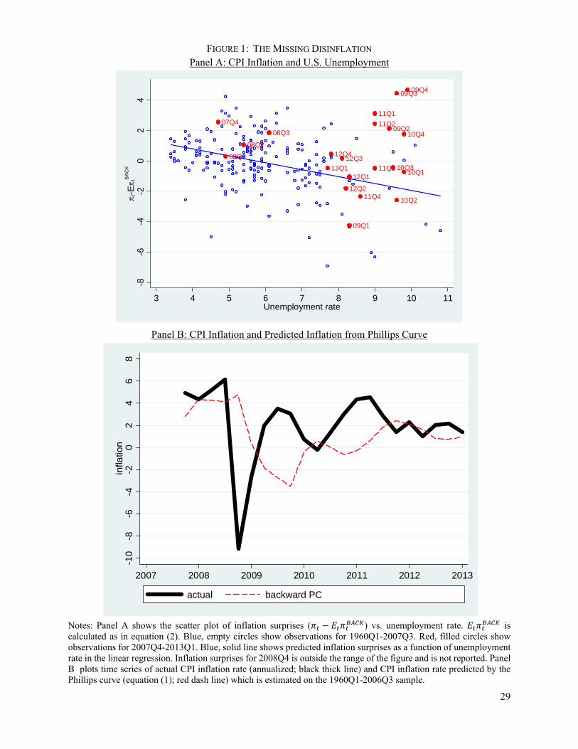
29
FIGURE 1: THE MISSING DISINFLATION Panel A: CPI Inflation and U.S. Unemployment
Panel B: CPI Inflation and Predicted Inflation from Phillips Curve
Notes: Panel A shows the scatter plot of inflation surprises ( ) vs. unemployment rate. is calculated as in equation (2). Blue, empty circles show observations for 1960Q1-2007Q3. Red, filled circles show observations for 2007Q4-2013Q1. Blue, solid line shows predicted inflation surprises as a function of unemployment rate in the linear regression. Inflation surprises for 2008Q4 is outside the range of the figure and is not reported. Panel B plots time series of actual CPI inflation rate (annualized; black thick line) and CPI inflation rate predicted by the Phillips curve (equation (1); red dash line) which is estimated on the 1960Q1-2006Q3 sample.
07Q4
08Q1
08Q2
08Q3
09Q1
09Q2
09Q309Q4
10Q1
10Q2
10Q3
10Q4
11Q1
11Q2
11Q3
11Q4
12Q1
12Q2
12Q312Q4
13Q1
-8-6
-4-2
02
4 t
-E t
BA
CK
3 4 5 6 7 8 9 10 11Unemployment rate
-10
-8-6
-4-2
02
46
8in
flatio
n
2007 2008 2009 2010 2011 2012 2013
actual backward PC
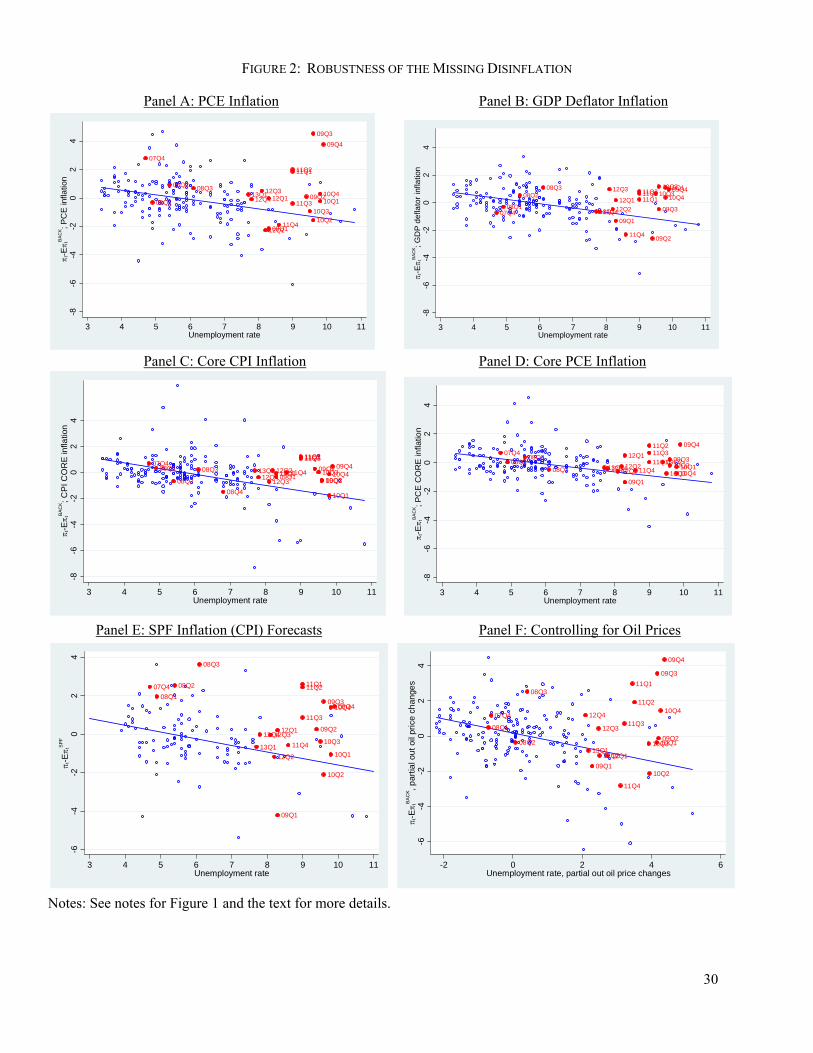
30
FIGURE 2: ROBUSTNESS OF THE MISSING DISINFLATION
Panel A: PCE Inflation Panel B: GDP Deflator Inflation
Panel C: Core CPI Inflation Panel D: Core PCE Inflation
Panel E: SPF Inflation (CPI) Forecasts Panel F: Controlling for Oil Prices
Notes: See notes for Figure 1 and the text for more details.
07Q408Q1
08Q2
08Q3
08Q4
09Q109Q2
09Q3
09Q4
10Q1
10Q210Q310Q4
11Q111Q211Q3
11Q412Q112Q2
12Q312Q4
13Q1
-8-6
-4-2
02
4 t
-E t
BA
CK; C
PI C
OR
E in
flatio
n
3 4 5 6 7 8 9 10 11Unemployment rate
07Q4
08Q1
08Q2
08Q3
09Q1
09Q2
09Q309Q4
10Q1
10Q2
10Q3
10Q4
11Q111Q2
11Q3
11Q4
12Q1
12Q2
12Q312Q4
13Q1
-6-4
-20
24
t-E t
SP
F
3 4 5 6 7 8 9 10 11Unemployment rate
07Q4
08Q1
08Q2
08Q3
09Q1
09Q2
09Q3
09Q4
10Q1
10Q2
10Q3
10Q4
11Q1
11Q2
11Q3
11Q4
12Q112Q2
12Q3
12Q4
13Q1
-6-4
-20
24
t-E t
BA
CK, p
artia
l ou
t oil
pric
e ch
ange
s
-2 0 2 4 6Unemployment rate, partial out oil price changes
07Q408Q1
08Q208Q3
09Q1
09Q2
09Q3
09Q410Q110Q210Q3
10Q411Q111Q211Q3
11Q4
12Q1
12Q2
12Q3
12Q413Q1
-8-6
-4-2
02
4 t
-E t
BA
CK; G
DP
def
lato
r in
flatio
n
3 4 5 6 7 8 9 10 11Unemployment rate
07Q408Q1
08Q2
08Q3
09Q1
09Q209Q3
09Q4
10Q110Q210Q310Q4
11Q1
11Q211Q3
11Q4
12Q1
12Q212Q312Q413Q1
-8-6
-4-2
02
4 t
-E t
BA
CK; P
CE
CO
RE
infla
tion
3 4 5 6 7 8 9 10 11Unemployment rate
07Q4
08Q1
08Q2 08Q3
09Q1
09Q2
09Q3
09Q4
10Q1
10Q210Q3
10Q4
11Q111Q2
11Q3
11Q4
12Q1
12Q2
12Q312Q4
13Q1
-8-6
-4-2
02
4 t
-E t
BA
CK; P
CE
infla
tion
3 4 5 6 7 8 9 10 11Unemployment rate
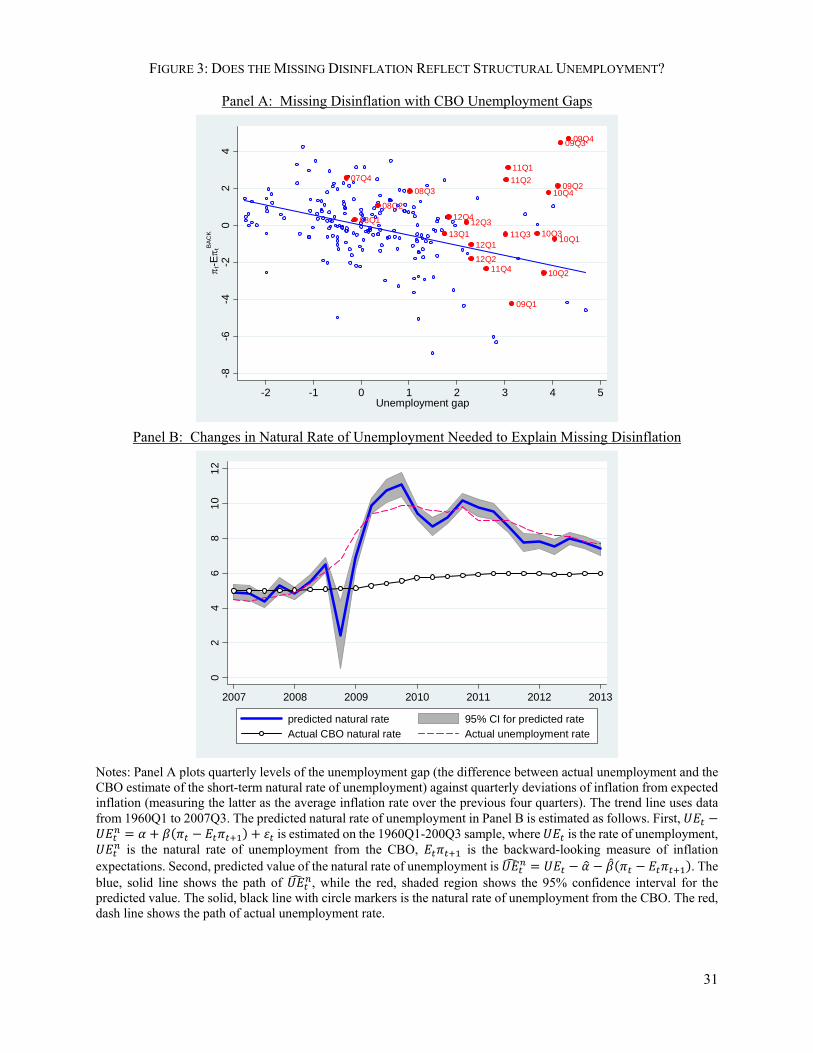
31
FIGURE 3: DOES THE MISSING DISINFLATION REFLECT STRUCTURAL UNEMPLOYMENT?
Panel A: Missing Disinflation with CBO Unemployment Gaps
Panel B: Changes in Natural Rate of Unemployment Needed to Explain Missing Disinflation
Notes: Panel A plots quarterly levels of the unemployment gap (the difference between actual unemployment and the CBO estimate of the short-term natural rate of unemployment) against quarterly deviations of inflation from expected inflation (measuring the latter as the average inflation rate over the previous four quarters). The trend line uses data from 1960Q1 to 2007Q3. The predicted natural rate of unemployment in Panel B is estimated as follows. First,
is estimated on the 1960Q1-200Q3 sample, where is the rate of unemployment, is the natural rate of unemployment from the CBO, is the backward-looking measure of inflation
expectations. Second, predicted value of the natural rate of unemployment is . The blue, solid line shows the path of , while the red, shaded region shows the 95% confidence interval for the predicted value. The solid, black line with circle markers is the natural rate of unemployment from the CBO. The red, dash line shows the path of actual unemployment rate.
07Q4
08Q1
08Q2
08Q3
09Q1
09Q2
09Q309Q4
10Q1
10Q2
10Q3
10Q4
11Q1
11Q2
11Q3
11Q4
12Q1
12Q2
12Q312Q4
13Q1-8
-6-4
-20
24
t-E t
BA
CK
-2 -1 0 1 2 3 4 5Unemployment gap
02
46
81
01
2
2007 2008 2009 2010 2011 2012 2013
predicted natural rate 95% CI for predicted rateActual CBO natural rate Actual unemployment rate
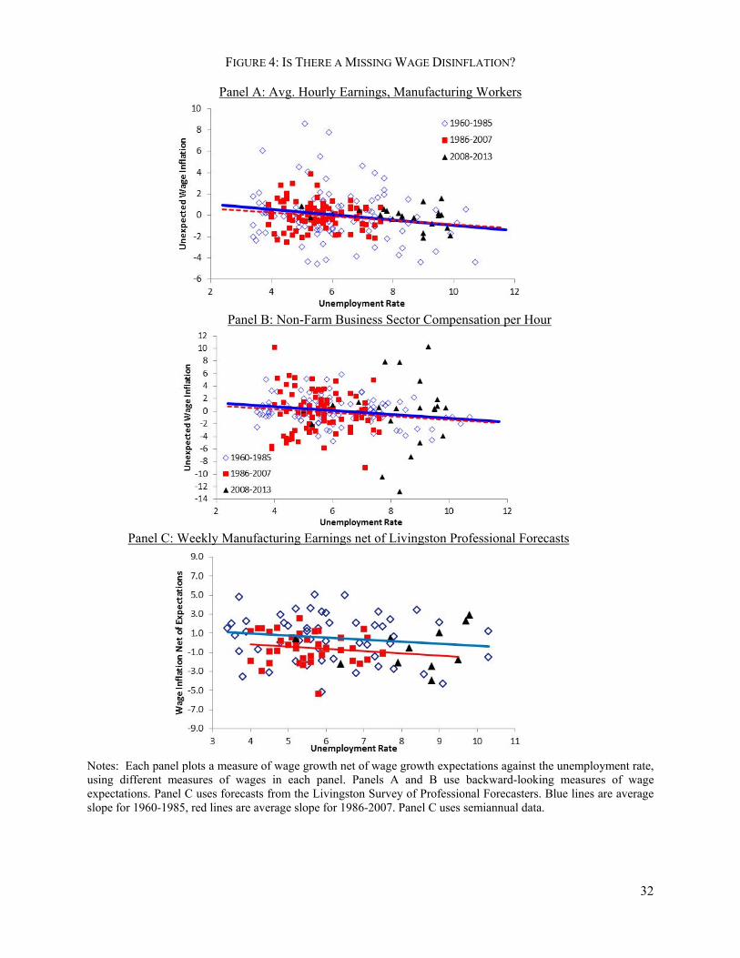
32
FIGURE 4: IS THERE A MISSING WAGE DISINFLATION?
Panel A: Avg. Hourly Earnings, Manufacturing Workers
Panel B: Non-Farm Business Sector Compensation per Hour
Panel C: Weekly Manufacturing Earnings net of Livingston Professional Forecasts
Notes: Each panel plots a measure of wage growth net of wage growth expectations against the unemployment rate, using different measures of wages in each panel. Panels A and B use backward-looking measures of wage expectations. Panel C uses forecasts from the Livingston Survey of Professional Forecasters. Blue lines are average slope for 1960-1985, red lines are average slope for 1986-2007. Panel C uses semiannual data.
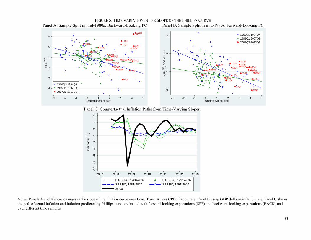
33
FIGURE 5: TIME VARIATION IN THE SLOPE OF THE PHILLIPS CURVE Panel A: Sample Split in mid-1980s, Backward-Looking PC Panel B: Sample Split in mid-1980s, Forward-Looking PC
Panel C: Counterfactual Inflation Paths from Time-Varying Slopes
Notes: Panels A and B show changes in the slope of the Phillips curve over time. Panel A uses CPI inflation rate. Panel B using GDP deflator inflation rate. Panel C shows the path of actual inflation and inflation predicted by Phillips curve estimated with forward-looking expectations (SPF) and backward-looking expectations (BACK) and over different time samples.
07Q4
08Q1
08Q2
08Q3
09Q1
09Q2
09Q309Q4
10Q1
10Q2
10Q3
10Q4
11Q1
11Q2
11Q3
11Q4
12Q1
12Q2
12Q312Q4
13Q1
-6-4
-20
24
t-E t
BA
CK
-3 -2 -1 0 1 2 3 4 5Unemployment gap
1960Q1-1984Q41985Q1-2007Q3
2007Q3-2013Q1
07Q4
08Q108Q2
08Q3
09Q1
09Q2
09Q3
09Q410Q110Q2
10Q310Q411Q111Q2
11Q3
11Q4
12Q1
12Q2
12Q3
12Q413Q1
-20
24
t-E t
SP
F, G
DP
de
flato
r
-3 -2 -1 0 1 2 3 4 5Unemployment gap
1960Q1-1984Q41985Q1-2007Q32007Q3-2013Q1
-10
-8-6
-4-2
02
46
infla
tion
(C
PI)
2007 2008 2009 2010 2011 2012 2013
BACK PC, 1960-2007 BACK PC, 1991-2007SPF PC, 1981-2007 SPF PC, 1991-2007actual
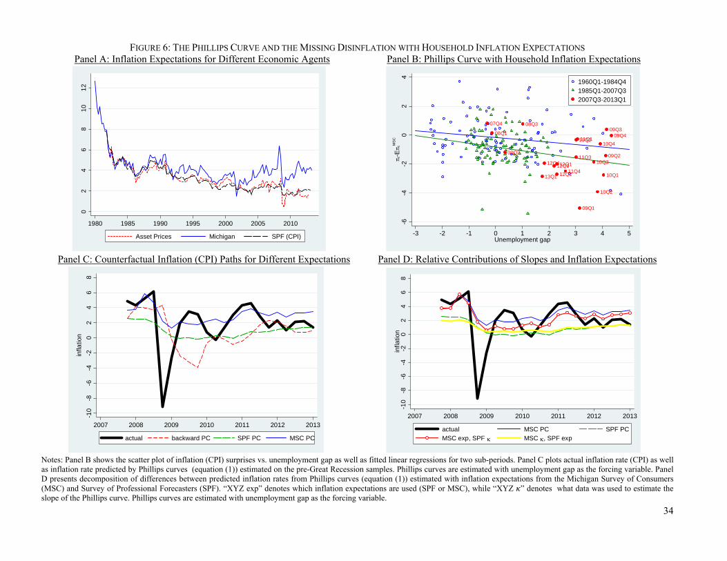
34
FIGURE 6: THE PHILLIPS CURVE AND THE MISSING DISINFLATION WITH HOUSEHOLD INFLATION EXPECTATIONS Panel A: Inflation Expectations for Different Economic Agents Panel B: Phillips Curve with Household Inflation Expectations
Panel C: Counterfactual Inflation (CPI) Paths for Different Expectations Panel D: Relative Contributions of Slopes and Inflation Expectations
Notes: Panel B shows the scatter plot of inflation (CPI) surprises vs. unemployment gap as well as fitted linear regressions for two sub-periods. Panel C plots actual inflation rate (CPI) as well as inflation rate predicted by Phillips curves (equation (1)) estimated on the pre-Great Recession samples. Phillips curves are estimated with unemployment gap as the forcing variable. Panel D presents decomposition of differences between predicted inflation rates from Phillips curves (equation (1)) estimated with inflation expectations from the Michigan Survey of Consumers (MSC) and Survey of Professional Forecasters (SPF). “XYZ exp” denotes which inflation expectations are used (SPF or MSC), while “XYZ ” denotes what data was used to estimate the slope of the Phillips curve. Phillips curves are estimated with unemployment gap as the forcing variable.
02
46
81
01
2
1980 1985 1990 1995 2000 2005 2010
Asset Prices Michigan SPF (CPI)
07Q4
08Q1
08Q2
08Q3
09Q1
09Q2
09Q309Q4
10Q1
10Q2
10Q3
10Q411Q111Q2
11Q3
11Q412Q1
12Q2
12Q312Q4
13Q1
-6-4
-20
24
t-E t
MS
C
-3 -2 -1 0 1 2 3 4 5Unemployment gap
1960Q1-1984Q41985Q1-2007Q32007Q3-2013Q1
-10
-8-6
-4-2
02
46
8
infla
tion
2007 2008 2009 2010 2011 2012 2013
actual backward PC SPF PC MSC PC
-10
-8-6
-4-2
02
46
8in
flatio
n
2007 2008 2009 2010 2011 2012 2013
actual MSC PC SPF PCMSC exp, SPF MSC , SPF exp
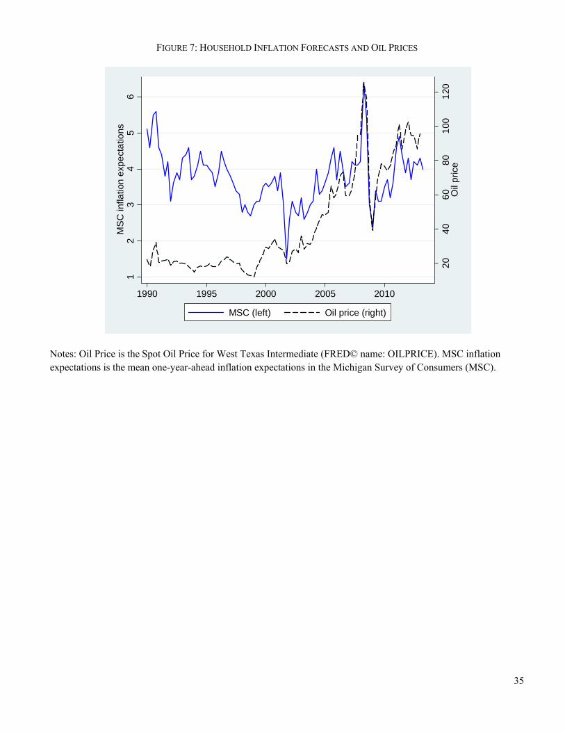
35
FIGURE 7: HOUSEHOLD INFLATION FORECASTS AND OIL PRICES
Notes: Oil Price is the Spot Oil Price for West Texas Intermediate (FRED© name: OILPRICE). MSC inflation expectations is the mean one-year-ahead inflation expectations in the Michigan Survey of Consumers (MSC).
2
04
06
08
01
001
20O
il p
rice
12
34
56
MS
C in
flatio
n e
xpe
cta
tions
1990 1995 2000 2005 2010
MSC (left) Oil price (right)
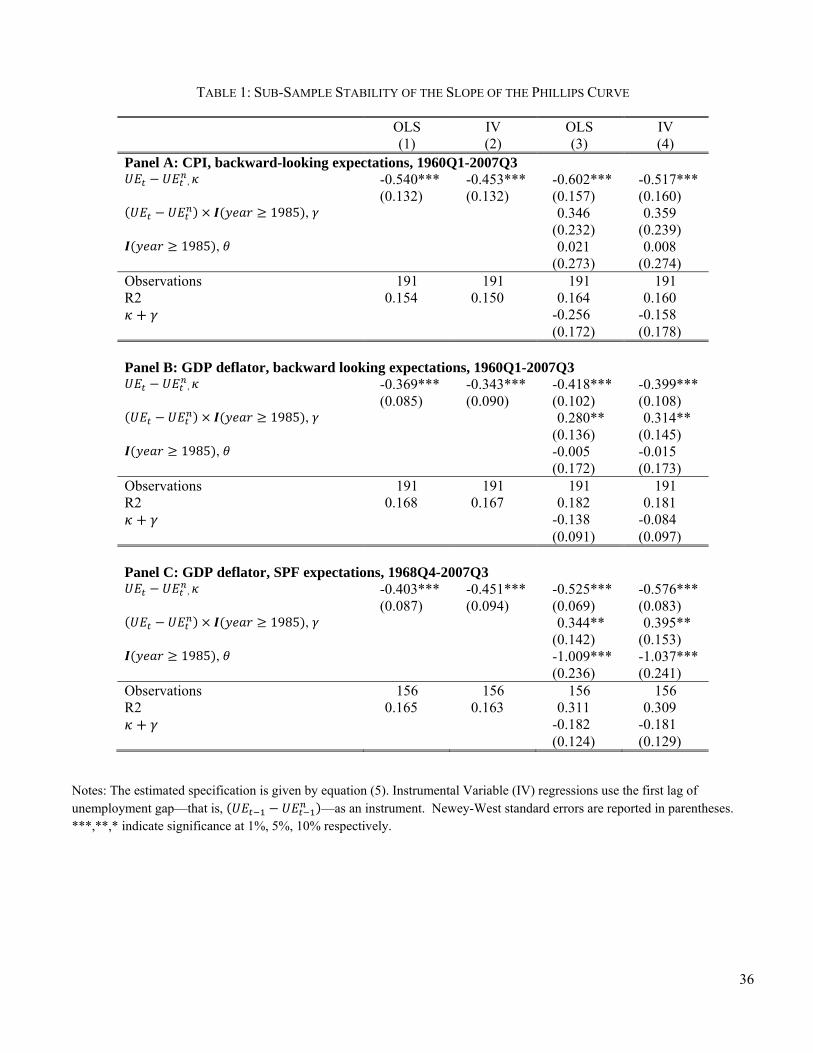
36
TABLE 1: SUB-SAMPLE STABILITY OF THE SLOPE OF THE PHILLIPS CURVE
OLS IV OLS IV (1) (2) (3) (4) Panel A: CPI, backward-looking expectations, 1960Q1-2007Q3
, -0.540*** -0.453*** -0.602*** -0.517*** (0.132) (0.132) (0.157) (0.160)
1985 , 0.346 0.359 (0.232) (0.239)
1985 , 0.021 0.008 (0.273) (0.274) Observations 191 191 191 191 R2 0.154 0.150 0.164 0.160
-0.256 -0.158 (0.172) (0.178) Panel B: GDP deflator, backward looking expectations, 1960Q1-2007Q3
, -0.369*** -0.343*** -0.418*** -0.399*** (0.085) (0.090) (0.102) (0.108)
1985 , 0.280** 0.314** (0.136) (0.145)
1985 , -0.005 -0.015 (0.172) (0.173) Observations 191 191 191 191 R2 0.168 0.167 0.182 0.181
-0.138 -0.084 (0.091) (0.097) Panel C: GDP deflator, SPF expectations, 1968Q4-2007Q3
, -0.403*** -0.451*** -0.525*** -0.576*** (0.087) (0.094) (0.069) (0.083)
1985 , 0.344** 0.395** (0.142) (0.153)
1985 , -1.009*** -1.037*** (0.236) (0.241) Observations 156 156 156 156 R2 0.165 0.163 0.311 0.309
-0.182 -0.181 (0.124) (0.129)
Notes: The estimated specification is given by equation (5). Instrumental Variable (IV) regressions use the first lag of unemployment gap—that is, —as an instrument. Newey-West standard errors are reported in parentheses. ***,**,* indicate significance at 1%, 5%, 10% respectively.
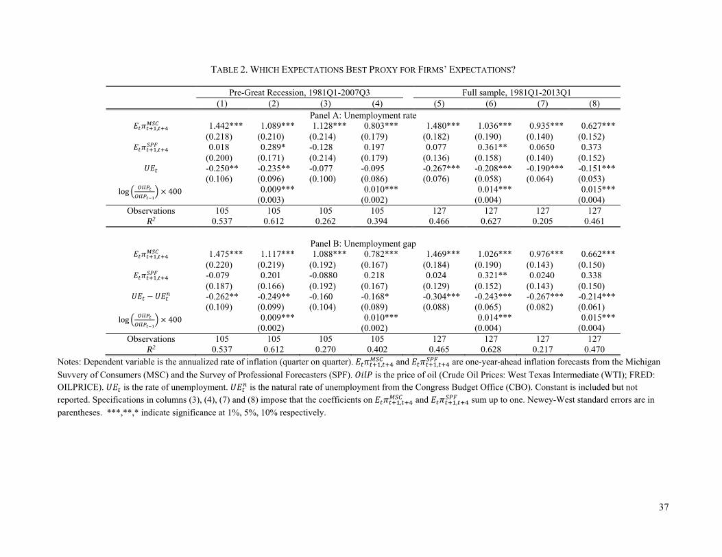
37
TABLE 2. WHICH EXPECTATIONS BEST PROXY FOR FIRMS’ EXPECTATIONS?
Pre-Great Recession, 1981Q1-2007Q3 Full sample, 1981Q1-2013Q1 (1) (2) (3) (4) (5) (6) (7) (8)
Panel A: Unemployment rate , 1.442*** 1.089*** 1.128*** 0.803*** 1.480*** 1.036*** 0.935*** 0.627***
(0.218) (0.210) (0.214) (0.179) (0.182) (0.190) (0.140) (0.152) , 0.018 0.289* -0.128 0.197 0.077 0.361** 0.0650 0.373
(0.200) (0.171) (0.214) (0.179) (0.136) (0.158) (0.140) (0.152) -0.250** -0.235** -0.077 -0.095 -0.267*** -0.208*** -0.190*** -0.151***
(0.106) (0.096) (0.100) (0.086) (0.076) (0.058) (0.064) (0.053) log 400 0.009*** 0.010*** 0.014*** 0.015***
(0.003) (0.002) (0.004) (0.004) Observations 105 105 105 105 127 127 127 127
R2 0.537 0.612 0.262 0.394 0.466 0.627 0.205 0.461
Panel B: Unemployment gap , 1.475*** 1.117*** 1.088*** 0.782*** 1.469*** 1.026*** 0.976*** 0.662***
(0.220) (0.219) (0.192) (0.167) (0.184) (0.190) (0.143) (0.150) , -0.079 0.201 -0.0880 0.218 0.024 0.321** 0.0240 0.338
(0.187) (0.166) (0.192) (0.167) (0.129) (0.152) (0.143) (0.150) -0.262** -0.249** -0.160 -0.168* -0.304*** -0.243*** -0.267*** -0.214***
(0.109) (0.099) (0.104) (0.089) (0.088) (0.065) (0.082) (0.061) log 400 0.009*** 0.010*** 0.014*** 0.015***
(0.002) (0.002) (0.004) (0.004) Observations 105 105 105 105 127 127 127 127
R2 0.537 0.612 0.270 0.402 0.465 0.628 0.217 0.470 Notes: Dependent variable is the annualized rate of inflation (quarter on quarter). , and , are one-year-ahead inflation forecasts from the Michigan
Suvvery of Consumers (MSC) and the Survey of Professional Forecasters (SPF). is the price of oil (Crude Oil Prices: West Texas Intermediate (WTI); FRED: OILPRICE). is the rate of unemployment. is the natural rate of unemployment from the Congress Budget Office (CBO). Constant is included but not reported. Specifications in columns (3), (4), (7) and (8) impose that the coefficients on , and , sum up to one. Newey-West standard errors are in
parentheses. ***,**,* indicate significance at 1%, 5%, 10% respectively.
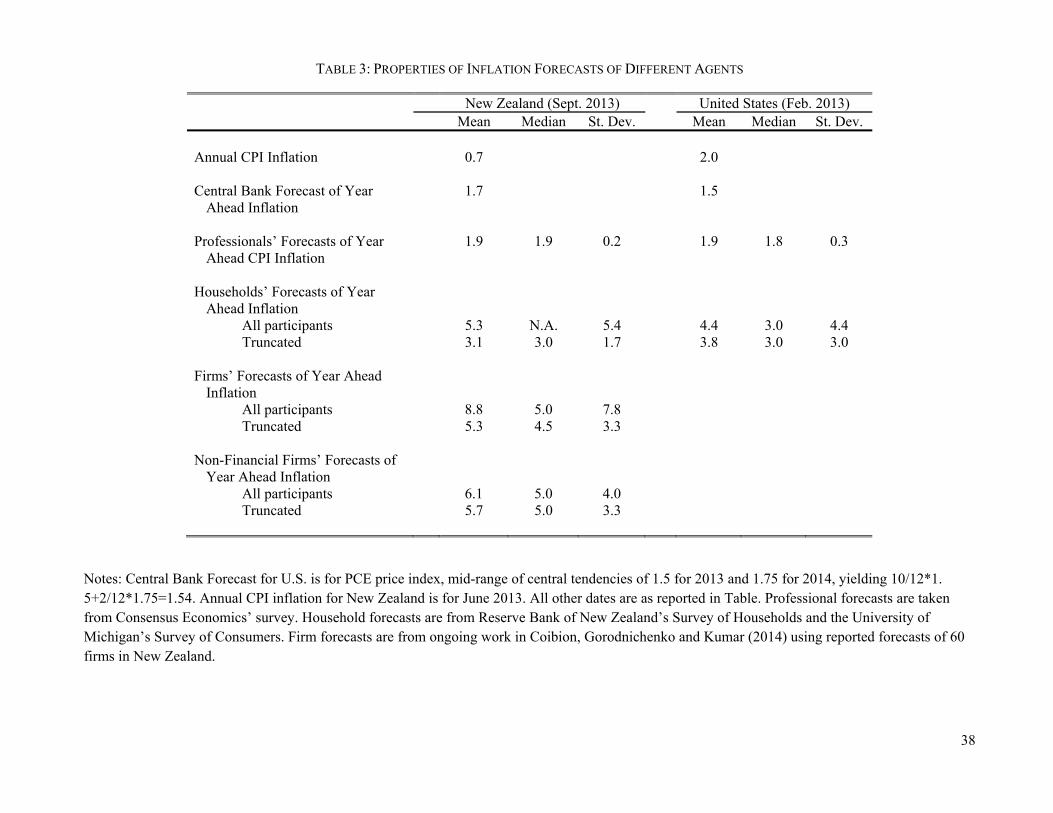
38
TABLE 3: PROPERTIES OF INFLATION FORECASTS OF DIFFERENT AGENTS
New Zealand (Sept. 2013) United States (Feb. 2013) Mean Median St. Dev. Mean Median St. Dev. Annual CPI Inflation 0.7 2.0 Central Bank Forecast of Year
Ahead Inflation 1.7 1.5
Professionals’ Forecasts of Year
Ahead CPI Inflation 1.9 1.9 0.2 1.9 1.8 0.3
Households’ Forecasts of Year
Ahead Inflation
All participants 5.3 N.A. 5.4 4.4 3.0 4.4 Truncated 3.1 3.0 1.7 3.8 3.0 3.0
Firms’ Forecasts of Year Ahead
Inflation
All participants 8.8 5.0 7.8 Truncated 5.3 4.5 3.3
Non-Financial Firms’ Forecasts of
Year Ahead Inflation
All participants 6.1 5.0 4.0 Truncated 5.7 5.0 3.3
Notes: Central Bank Forecast for U.S. is for PCE price index, mid-range of central tendencies of 1.5 for 2013 and 1.75 for 2014, yielding 10/12*1. 5+2/12*1.75=1.54. Annual CPI inflation for New Zealand is for June 2013. All other dates are as reported in Table. Professional forecasts are taken from Consensus Economics’ survey. Household forecasts are from Reserve Bank of New Zealand’s Survey of Households and the University of Michigan’s Survey of Consumers. Firm forecasts are from ongoing work in Coibion, Gorodnichenko and Kumar (2014) using reported forecasts of 60 firms in New Zealand.
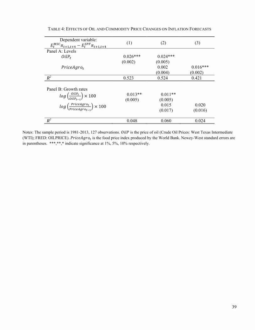
39
TABLE 4: EFFECTS OF OIL AND COMMODITY PRICE CHANGES ON INFLATION FORECASTS
Dependent variable:
, , (1) (2) (3)
Panel A: Levels 0.026*** 0.024***
(0.002) (0.005) 0.002 0.016***
(0.004) (0.002) R2 0.523 0.524 0.421
Panel B: Growth rates
100 0.013** 0.011** (0.005) (0.005)
100 0.015 0.020 (0.017) (0.016)
R2 0.048 0.060 0.024 Notes: The sample period is 1981-2013, 127 observations. is the price of oil (Crude Oil Prices: West Texas Intermediate (WTI); FRED: OILPRICE). is the food price index produced by the World Bank. Newey-West standard errors are in parentheses. ***,**,* indicate significance at 1%, 5%, 10% respectively.
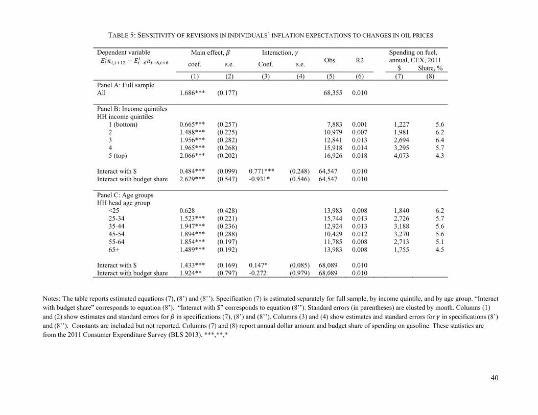
40
TABLE 5: SENSITIVITY OF REVISIONS IN INDIVIDUALS’ INFLATION EXPECTATIONS TO CHANGES IN OIL PRICES
Dependent variable
, , Main effect, Interaction,
Obs. R2 Spending on fuel,
annual, CEX, 2011 coef. s.e. Coef. s.e.
$ Share, %
(1) (2) (3) (4) (5) (6) (7) (8) Panel A: Full sample All
1.686*** (0.177) 68,355 0.010
Panel B: Income quintiles HH income quintiles
1 (bottom) 0.665*** (0.257) 7,883 0.001 1,227 5.6 2 1.488*** (0.225) 10,979 0.007 1,981 6.2 3 1.956*** (0.282) 12,841 0.013 2,694 6.4 4 1.965*** (0.268) 15,918 0.014 3,295 5.7 5 (top) 2.066*** (0.202) 16,926 0.018 4,073 4.3
Interact with $ 0.484*** (0.099) 0.771*** (0.248) 64,547 0.010 Interact with budget share
2.629*** (0.547) -0.931* (0.546) 64,547 0.010
Panel C: Age groups HH head age group
<25 0.628 (0.428) 13,983 0.008 1,840 6.2 25-34 1.523*** (0.221) 15,744 0.013 2,726 5.7 35-44 1.947*** (0.236) 12,924 0.013 3,188 5.6 45-54 1.894*** (0.288) 10,429 0.012 3,270 5.6 55-64 1.854*** (0.197) 11,785 0.008 2,713 5.1 65+ 1.489*** (0.192) 13,983 0.008 1,755 4.5
Interact with $ 1.433*** (0.169) 0.147* (0.085) 68,089 0.010 Interact with budget share 1.924** (0.797) -0.272 (0.979) 68,089 0.010
Notes: The table reports estimated equations (7), (8’) and (8’’). Specification (7) is estimated separately for full sample, by income quintile, and by age group. “Interact with budget share” corresponds to equation (8’). “Interact with $” corresponds to equation (8’’). Standard errors (in parentheses) are clusted by month. Columns (1) and (2) show estimates and standard errors for in specifications (7), (8’) and (8’’). Columns (3) and (4) show estimates and standard errors for in specifications (8’) and (8’’). Constants are included but not reported. Columns (7) and (8) report annual dollar amount and budget share of spending on gasoline. These statistics are from the 2011 Consumer Expenditure Survey (BLS 2013). ***,**,*

41
APPENDIX FIGURES AND TABLES
42
APPENDIX TABLE 1. HOUSEHOLD VS. BACKWARD-LOOKING EXPECTATIONS IN ESTIMATED PHILLIPS CURVES.
Pre-Great Recession, 1960Q1-2007Q3 Full sample, 1960Q1-2013Q1 (1) (2) (3) (4) (5) (6) (7) (8)
Panel A: Unemployment rate , 1.126*** 0.993*** 0.761*** 0.698*** 1.303*** 1.041*** 0.865*** 0.730***
(0.099) (0.079) (0.077) (0.065) (0.174) (0.091) (0.123) (0.068) , 0.158** 0.224*** 0.239*** 0.302*** 0.025 0.175** 0.135 0.270***
(0.079) (0.064) (0.077) (0.065) (0.129) (0.071) (0.123) (0.068) -0.238*** -0.207*** -0.162** -0.144* -0.238*** -0.203*** -0.189*** -0.167***
(0.072) (0.070) (0.080) (0.074) (0.058) (0.050) (0.062) (0.052) log 400 0.008*** 0.011*** 0.012*** 0.015***
(0.002) (0.002) (0.004) (0.004) Observations 191 191 191 191 213 213 213 213
R2 0.846 0.864 0.456 0.558 0.786 0.830 0.434 0.590
Panel B: Unemployment gap , 1.097*** 0.962*** 0.743*** 0.684*** 1.279*** 1.017*** 0.873*** 0.740***
(0.097) (0.077) (0.076) (0.062) (0.172) (0.090) (0.129) (0.072) , 0.157** 0.228*** 0.257*** 0.316*** 0.020 0.173** 0.127 0.260***
(0.076) (0.061) (0.076) (0.062) (0.130) (0.072) (0.129) (0.072) -0.270*** -0.247*** -0.279*** -0.247*** -0.272*** -0.244*** -0.285*** -0.247***
(0.079) (0.075) (0.087) (0.079) (0.067) (0.055) (0.076) (0.058) log 400 0.008*** 0.011*** 0.012*** 0.015***
(0.002) (0.002) (0.004) (0.004) Observations 191 191 191 191 213 213 213 213
R2 0.847 0.866 0.479 0.575 0.788 0.833 0.454 0.604
Notes: Dependent variable is the annualized rate of inflation (quarter on quarter). , and , are one-year-ahead inflation forecasts from the Michigan Survey of
Consumers (MSC) and backward-looking forecasts as described in equation (2) in the text. is the price of oil (Crude Oil Prices: West Texas Intermediate (WTI); FRED: OILPRICE). is the rate of unemployment. is the natural rate of unemployment from the Congress Budget Office (CBO). Constant is included but not reported. Specifications in columns (3), (4), (7) and (8) impose that the coefficients on , and , sum up to one. Newey-West standard errors are in parentheses. ***,**,*
indicate significance at 1%, 5%, 10% respectively.
43
APPENDIX FIGURE 1. TIME SERIES OF SELECTED MACROECONOMIC VARIABLES Panel A: Index of labor share, Nonfarm Business Sector (FRED© code: PRS85006173)
Panel B. Ratio of Corporate Profits (FRED© code: CP) to GDP (FRED© code: GDP)
95
100
105
110
115
lab
or s
hare
1960 1970 1980 1990 2000 2010
46
81
01
2C
orp
ora
te P
rofit
/GD
P
1960 1970 1980 1990 2000 2010