Is There a Speculative Bubble in the Price of Gold

Is There a Speculative Bubble in the Price of Gold?∗

Jedrzej P. Bialkowski, Martin T. Bohl†, Patrick M. Stephan andTomasz P. Wisniewski

January 4, 2012

Abstract

Motivated by the current gold price boom, this paper investigates whether rapidly

growing investment activities have caused a new asset price bubble. Drawing on

gold’s role as dollar hedge, inflation hedge, portfolio diversifier and safe haven,

we calculate fundamentally justified returns and approximate gold’s fundamen-

tal value. Based on the deviations of the actual gold price from its fitted value,

we then apply a Markov regime-switching Augmented Dickey-Fuller (ADF) test,

which has substantial power for detecting explosive behavior. However, our em-

pirical evidence is favorable for a fundamentally justified price level even during

the current period where the gold price is rising dramatically.

JEL Classification: G10, G11, G12, G18

Keywords: Gold Price, Speculative Bubble, Markov Regime-Switching ADF Test

∗We are indebted to participants of the 15th New Zealand Finance Colloquium in Christchurch,New Zealand, the 2nd Finance and Corporate Governance Conference in Melbourne, Australia, the15th International Conference on Macroeconomic Analysis and International Finance in Rethymno,Greece, the 9th Infiniti Conference on International Finance in Dublin, Ireland, the 18th AnnualMeeting of the Multinational Finance Society in Rome, Italy, the 86th Annual Conference of theWestern Economic Association International in San Diego, USA, the 2011 Annual Meeting of theGerman Economic Association in Frankfurt/Main, Germany, the 5th International Conference onComputational and Financial Econometrics in London, Great Britain, and the research seminar ofthe Chair of Monetary Economics of the Westphalian Wilhelminian University of Munster, Germany,especially to Dirk Baur, Jorg Breitung, Levan Efremidze, Philipp Kaufmann, Arne Klein, JudithLischewski, Brian Lucey, Dimitris Psychoyios, Jana Riedel, Kashif Saleem, Christian Salm, MichaelSchuppli, Rainer Schussler and Jiri Svec, for helpful comments and suggestions.†Corresponding author: Department of Economics, Westphalian Wilhelminian University of

Munster, Am Stadtgraben 9, 48143 Munster, Germany, Phone: +49 251 83 25005, Fax: +49 25183 22846, E-mail address: [email protected] (Martin T. Bohl)

1

1

1. Introduction and Literature Review

Since 2001, the price of gold has skyrocketed from a level of US$ 250 per troy ounce to

an all-time high of US$ 1,900 in August 2011, before falling slightly. On the one hand,

this development might be fundamentally justified by the increasingly important role of

gold as dollar hedge (Sjaastad and Scacciavillani, 1996; Capie et al., 2005;

Tully and Lucey, 2007; Pukthuanthong and Roll, 2011), inflation hedge

(Adrangi et al., 2003; Worthington and Pahlavani, 2007; Blose, 2010)

and portfolio diversifier (Jaffe, 1989; Hillier et al., 2006). In addition, gold is

regarded as a safe haven (Baur and Lucey, 2010; Baur and McDermott, 2010;

Chan et al., 2011), especially in times of the recent world financial and the current

European sovereign debt crisis. On the other hand, gold’s growing attractiveness as an

investment asset and the gold price boom might indicate a speculative bubble.1

Phillips and Yu (2010) find evidence for a speculative bubble moving from the

equity market (up to 2000) over the US housing market (up to 2007) to the crude oil

market (up to mid-2008). Thus, we ask whether the gold market is another victim of

such a wandering asset price bubble. If this is indeed the case, gold market participants

will run the risk of experiencing huge losses once the bubble bursts. So far, to the best

of our knowledge, the possibility that the gold price may currently exhibit a speculative

bubble has been largely neglected by the academic literature. The present paper aims

to fill this gap by applying an econometric technique which allows for early detection

of speculative bubbles. Thus, we are able to offer insights not only for academics

and investors, but also for decision makers engaged in fighting speculative bubbles by

framing early monetary policy responses or other regulatory interventions.

Until now, econometric testing for speculative bubbles has mainly been focused on

(US) stock markets. Gurkaynak (2008) provides a recent in-depth survey of econo-

1According to the World Gold Council (2010), the estimated global demand for gold of netretail investors rose from 166 tonnes in 2000 to 731 tonnes in 2009. Simultaneously, exchange-tradedfunds (ETFs) increased their demand from basically nothing to 617 tonnes. For further informationon the global gold market see, for instance, Shafiee and Topal (2010).

2

metric methods used for detecting asset price bubbles. This survey includes the well-

known variance bounds tests, West’s two-step method, (co)integration-based tests as

well as the concept of intrinsic bubbles and methods treating bubbles as an unobserved

variable. By contrast, little effort has been made to date in identifying speculative bub-

bles in the gold price. Blanchard and Watson (1982) draw on runs and tail tests,

but are unable to conclude whether the gold price was unjustifiably high between 1975

and 1981, given the caveats of their methodology. Diba and Grossman (1984) in-

vestigate the stationarity properties of the gold price for the time period from 1975 to

1983, and find that it was entirely based on market fundamentals.

As shown by Evans (1991), however, the ordinary unit-root and cointegration tests

do not allow for the detection of the important class of periodically bursting bubbles.

Due to the bursting nature of such bubbles, these tests have a tendency to reject the null

hypothesis of non-stationarity in favor of the stationary alternative all too often. Being

aware of this critique, Pindyck (1993) draws on the convenience yield approach, and

calculates gold’s fundamental value based on the present value model for commodities.

Running tests of forecasting power, Granger causality and restrictions of appropriately

specified vector autoregressive (VAR) models, Pindyck (1993) finds evidence in favor

of gold price bubbles between 1975 and 1990. Finally, based on a dynamic factor model,

Bertus and Stanhouse (2001) focus on the gold futures market, and provide weak

evidence for gold price bubbles during notable socioeconomic events in the time period

from 1975 to 1998.

With regard to the current gold price boom, only two studies provide preliminary

empirical evidence. Went et al. (2009) build on the convenience yield model, and

run the duration dependence test which indicates gold price bubbles in the time span

from 1976 to 2005. Unfortunately, their approach suffers from the fact that they cannot

conclude when speculative bubbles affected the gold price exactly. In addition, Homm

and Breitung (2011) use the supplemented Augmented Dickey-Fuller (ADF) test,

3

and find evidence for gold price bubbles between 1968 and 1980 (at the 1%-level) and

between 1984 and 2010 (at the 10%-level). However, their methodology only tests

for explosiveness in the price time series itself, and does not take gold’s fundamental

factors into consideration. As a consequence, Homm and Breitung (2011) are thus

unable to conclude whether their findings might result from major economic events

such as the current European sovereign debt crisis rather than speculative excess.

In order to overcome these caveats, we propose to construct gold’s fundamental value

making use of its role as dollar hedge, inflation hedge, portfolio diversifier and safe

haven. Drawing on the deviations of the actual gold price from its fitted value, we then

apply a Markov regime-switching ADF test to identify periods that are characterized by

explosive behavior. Based on estimated probabilities of being in the possible bubble and

the non-bubble regime, this approach thus also allows for the detection of speculative

bubbles in most recent times. However, the use of this methodology meant that we

could find no empirical evidence of speculative bubbles either for the gold price boom

from 1979 to 1982 or in most recent times. In addition, we find that the European

sovereign debt crisis can be seen as the major reason for the current gold price boom.

The paper proceeds as follows. In Section 2, we discuss the construction of gold’s

fundamental value. In Section 3, we explain the Markov regime-switching ADF test.

In Section 4, we show our empirical results. In Section 5, we briefly conclude.

2. Construction of Gold’s Fundamental Value

As outlined above, gold is widely regarded as dollar hedge, inflation hedge, portfolio

diversifier and safe haven. First, if gold is a hedge against the dollar, its price should

be inversely related to the strength of the US currency. Second, if gold is a hedge

against inflation, its price should comove with the price index of a basket of goods, so

that gold’s real value is preserved. Third, if gold is a portfolio diversifier (safe haven)

against financial assets such as stocks and bonds, its price should be uncorrelated or

negatively correlated with them (in times of market turmoil).

4

Based on these possible fundamental factors of the gold price, we explain its return

at date t, rGold,t, as follows:

rGold,t =2∑

i=0

γ1,i · rFX,t−i +2∑

i=0

γ2,i · rInflation,t−i +2∑

i=0

γ3,i · rMSCI,t−i +

2∑i=0

γ4,i · rT−Bill,t−i +2∑

i=0

γ5,i · rSpread,t−i + νt, (1)

where rFX,t is the change of the trade-weighted value of the US Dollar against other

major currencies, rInflation,t is the change of the US all-urban consumer price index,

rMSCI,t is the change of the MSCI World index of major stock markets, rT−Bill,t is the

3-month US Treasury bill rate, rSpread,t is the spread between the 10-year government

bond yield of Greece and Germany, and νt is the error term. rFX,t refers to gold’s role

as dollar hedge, rInflation,t should capture its role as inflation hedge, and the selection

of rMSCI,t, rT−Bill,t and rSpread,t is motivated by gold’s role as portfolio diversifier in

tranquil periods and as safe haven in times of market turmoil.

All regressors are allowed to have a contemporaneous and a lagged impact of one

and two periods. Time series which contain a unit root are adjusted by subtracting

the respective variable’s mean value of the previous year. All variables are calculated

as continuous changes in percent and refer to the last day of a month, except for the

inflation rate which is only available on a monthly frequency anyway. All (adjusted)

time series consist of 442 observations (Jan. 1975 – Oct. 2011), except for the spread

between the 10-year government bond yield of Greece and Germany, which includes

106 observations (Jan. 2003 – Oct. 2011). Thus, the latter variable explicitly captures

the possible influence of the current European sovereign debt crisis on the gold return.

All time series are taken from Thomson Reuters Datastream.

We distinguish between three different models. Model A refers to the shortened

sample from Jan. 1975 to Dec. 2007 (396 observations), excluding the spread between

Greek and German bond yields in order to calculate gold’s fundamental return. Model

5

B refers to the full sample, again excluding the yield spread. Finally, Model C also

refers to the full sample, but includes the yield spread.

Since we do not expect gold’s role as dollar hedge, inflation hedge, portfolio diversifier

and safe haven to be constant over time, we apply a rolling window approach. The

first window covers the period from Mar. 1975 to Feb. 1980, and is used to calculate

fitted gold returns, rGold,t, for this time span. The window is then rolled forward by

one month, so that new parameter estimates and a fitted gold return can be obtained

for Mar. 1980. For Model(s) A (B and C), the procedure is continued until Dec. 2007

(Oct. 2011), resulting in 335 (381) sets of OLS estimates.2

Finally, we calculate gold’s fundamental value by multiplying its actual price in Feb.

1975 with the fitted gross return of Mar. 1975, ending up with a fitted gold price for

the latter month. Afterwards, we multiply this fitted price with the fitted gross return

of Apr. 1975, and repeat this exercise until Dec. 2007 in the case of Model A, and

until Oct. 2011 in the case of Models B and C, respectively (Pt = Pt−1 · (1 + rGold,t)).

Deviations of the actual gold price from its fitted value (ut = Pt − Pt) are interpreted

as overvaluation if positive and as undervaluation if negative, respectively.

3. Markov Regime-Switching ADF Test for Bubble Detection

Based on the relationship between the actual gold price and its fitted value, we test

for speculative bubbles in the former, extending the conventional ADF equation to a

standard two-state first-order Markov regime-switching model. In the literature, this

approach has mostly been carried out to analyze directly the stationarity properties of

the time series under investigation (Funke et al., 1994; Hall et al., 1999). By

contrast, we use the Markov regime-switching ADF test with respect to the deviations

of the actual gold price from its fitted value. The main advantage of this approach is

that it does not rest on an informal comparison of the switching patterns of different

2Alternatively, we add a constant to eq. (1) and repeat the rolling regression approach. Thefundamentally justified gold return is then defined as the fitted return minus the constant. However,results (not shown, but available upon request) are qualitatively the same as for the model in eq. (1).

6

time series, but allows for solid statistical inference. If periodically bursting bubbles

exist, we should be able to distinguish between a moderately growing regime on the

one hand and an explosive and then collapsing regime on the other hand.3 As shown

by a simulation study in Hall et al. (1999), the Markov regime-switching ADF

test has substantially more power than the conventional ADF test in order to detect

peridocially bursting bubbles.

The Markov regime-switching ADF equation reads:

∆ut = ρ0,St + ρ1,St · ut−1 +

p∑k=1

βk,St ·∆ut−k + εSt , (2)

where ∆ stands for the first difference, St = (0, 1) is the stochastic regime variable, ψ ≡

(ρ0,St , ρ1,St , βk,St)′, with k = 1, . . . , p, are the regime-specific regression coefficients, and

εSt

i.i.d.∼ N(0, σ2St

) represents the error term. Judgments on the statistical significance of

the regression coefficients are based on critical values obtained by using a parametric

bootstrap algorithm (Psaradakis, 1998). If we are able to distinguish between a

bubble and a non-bubble regime, we will obtain one ρ1,i, i ∈ [0; 1], which is statistically

significantly bigger than zero (so that regime i is explosive and then collapsing), and

another ρ1,j, j = (1− i), which is not (so that regime j is stationary or contains a unit-

root). In order to ensure that the error terms are serially uncorrelated, the optimal lag

length, p, is determined by starting with pmax = [T (1/3)], where [·] denotes the integer

part of its argument, and then reducing the model until the last lagged difference has

a statistically significant influence at the 5%-level in at least one regime (general-to-

specific approach). Since the probability of St being either zero or one depends on the

past only through the most recent regime St−1, the transition probabilities are defined

by p00 ≡ Pr(St = 0|St−1 = 0) and p11 ≡ Pr(St = 1|St−1 = 1). Finally, we collect all

unknown parameters in the vector θ ≡ (ψ, σSt , p00, p11)′.

3Note that Markov regime-switching models may indicate different regimes even though there areno structural breaks in the data. Thus, we first apply a conventional ADF test to the deviations ofthe actual gold price from its fitted value, and test the stability of the ADF coefficient making use ofthe Quandt-Andrews unknown breakpoint tests.

7

In order to estimate θ, we draw on the expectation-maximization (EM) algorithm.

The EM algorithm is an iterative procedure that consists of two steps: the expectation

step and the maximization step (Hamilton, 1994; Kim and Nelson, 2000). In the

expectation step, we estimate the filter probabilities, Pr(St = i|ut, . . . , u1; θ), and the

smoothed probabilities, Pr(St = i|uT , . . . , u1; θ), of being in the two regimes, using the

estimate of θ from the previous iteration step. In the maximization step, we then draw

on these probabilities in order to improve the estimate of θ based on the maximum-

likelihood (ML) approach. Given the model in eq. (2), however, we need not maximize

the log-likelihood function numerically, but are able to obtain a closed-form solution

for θ. Furthermore, the EM algorithm is relatively robust with respect to poorly chosen

starting values for θ, quickly moving to a reasonable region of the likelihood surface.

4. Empirical Results

4.1. Descriptive Statistics

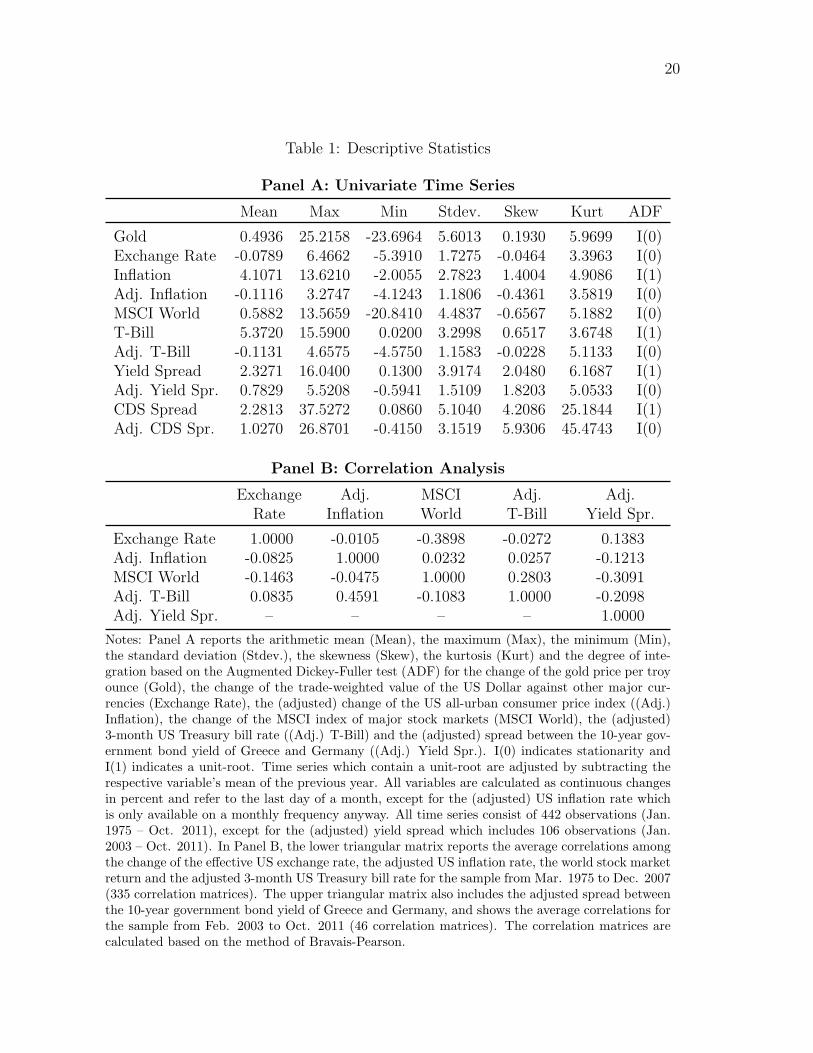
We start the empirical analysis by calculating descriptive statistics of the univariate

time series necessary to estimate eq. (1), based on the samples as described in Section

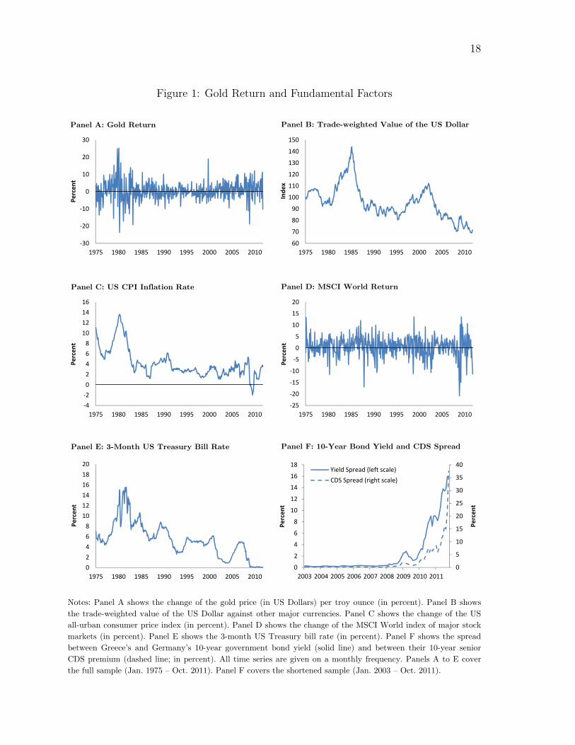
2. As shown by Panel A of Table 1, the largest positive gold return is more than 25

percent, and occurred during the last gold price boom in Feb. 1980, followed closely

by the largest negative return of more than 23 percent in Apr. 1980. In addition,

the largest value of the US inflation rate is more than 13 percent, and was measured

during the second oil crisis in Mar. 1980. Apart from this, world stock markets faced

their largest decrease of more than 20 percent in Nov. 2008, reflecting the recent world

financial crisis. Finally, the spread between the 10-year government bond yield of

Greece and Germany, which was always positive but skyrocketed over the last couple

of years, reached its peak of more than 16 percent in Oct. 2011, highlighting the current

European sovereign debt crisis. Figure 1 gives a visual impression of the (original)

time series used for our empirical analysis.

8

[Figure 1 about here]

More important, as indicated by the conventional ADF test, the gold return, the

change of the effective US exchange rate and the world stock market return are sta-

tionary, while the US inflation rate, the 3-month US Treasury bill rate and the spread

between Greek and German bond yields are characterized by a unit-root. Thus, we

adjust the latter three time series by subtracting the respective variable’s mean value

of the previous year in order to make them suitable for use in the regression in eq. (1).

[Table 1 about here]

Based on the rolling window approach, Panel B of Table 1 shows the average

correlations among the (stationary) fundamental factors of the gold return. As in

the regression analysis (see Section 4.2), the first window covers the period from

Mar. 1975 to Feb. 1980, and is then rolled forward by one month, so that a new

correlation matrix can be obtained. In the lower triangular matrix, we report the

average correlations among the change of the effective US exchange rate, the adjusted

US inflation rate, the world stock market return and the adjusted 3-month US Treasury

bill rate for the window rolling through the sample from Mar. 1975 to Dec. 2007 (335

correlation matrices). In the upper triangular matrix, we add the adjusted spread

between the 10-year government bond yield of Greece and Germany, and show the

average correlations for the window rolling through the sample from Feb. 2003 to

Oct. 2011 (46 correlation matrices). Since all average correlations among the five

fundamental factors are quite low, we conclude that multicollinearity does not disturb

the regression analysis.

4.2. Regression Results

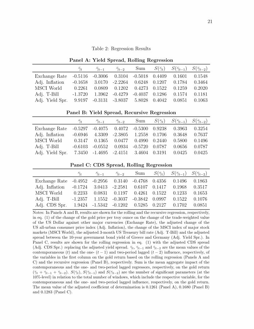
In Panel A of Table 2, we show the results of the rolling window approach used to

estimate the time-varying impact of the five fundamental factors on the gold return.

9

Instead of reporting the parameter estimates for each window, we focus on the mean

values of the contemporaneous and the one- and two-period lagged influence. In addi-

tion, we calculate the mean aggregate impact of the contemporaneous and the lagged

regressors. As expected, the gold return is negatively affected by the change of the

effective US exchange rate and the adjusted 3-month US Treasury bill rate, but has a

positive relationship with the adjusted US inflation rate and, in particular, with the

adjusted spread between the 10-year government bond yield of Greece and Germany.

Only the consistently positive influence of the world stock market return does not coin-

cide with gold’s role as portfolio diversifier. Finally, we show the number of significant

parameters in relation to the total number of windows, which include the respective

variable, for the contemporaneous and the lagged influence on the gold return. Overall,

the ratios indicate that the regressors selected serve as reasonable proxies in order to

reflect gold’s role as dollar hedge, inflation hedge, portfolio diversifier and safe haven.


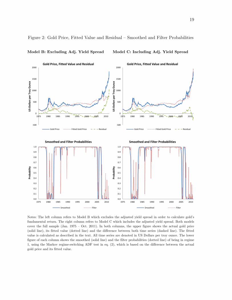
Based on the fitted gold returns, we then calculate gold’s fundamental value as

outlined in Section 2, and put it in relation to the actual gold price. Both time series

and the deviations of the actual gold price from its fitted value are shown in the upper

part of Figure 2. The figure in the left column refers to Model B which excludes the

adjusted spread between Greek and German bond yields in order to calculate gold’s

fundamental return, while the figure in the right column refers to Model C which

includes the yield spread. Interestingly, both figures indicate a persistent overvaluation

of the gold price in the first half of the 1980s, but differ sharply with respect to most

recent times. While Model B suggests a substantial overvaluation over the last few

years, Model C leads to a close co-movement of the actual gold price and its fitted

value. As a consequence, we argue that the current European sovereign debt crisis

might be seen as the major reason for the current gold price boom.

10

[Figure 2 about here]

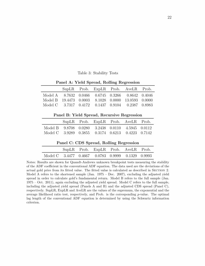
In order to validate this visual evidence empirically, we turn to the econometric

analysis of the deviations of the actual gold price from its fitted value. Using these

deviations, we first estimate the conventional ADF equation and test the stability of

the ADF coefficient by making use of the Quandt-Andrews unknown breakpoint tests.

Results for Models A, B and C are reported in Panel A of Table 3. Interestingly, they

indicate that only in case of Model B do the deviations of the actual gold price from

its fitted value appear to show different adjustment dynamics over time. By contrast,

no such instability of the ADF coefficient can be detected for Models A and C. Since

the conventional ADF test does not display explosive behavior for the full sample of

any model, we conclude that only Model B may lead to (relatively short) periods of

speculative bubbles.


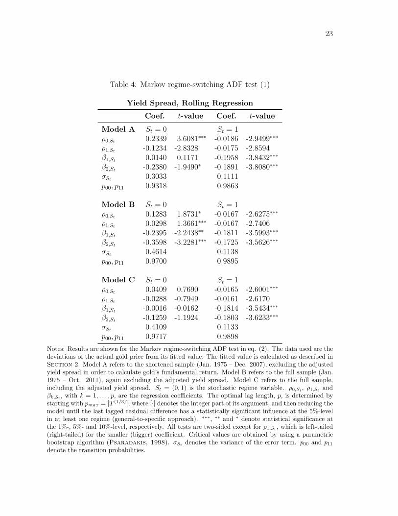
As a consequence, we further conclude that analyzing the deviations of the actual

gold price from its fitted value in case of Model B requires the Markov regime-switching

ADF test from eq. (2). For reasons of comparison, we also run this bubble test for

Models A and C. Results for all three models are reported in Table 4. Interestingly,

they have some characteristics in common. First, the constant is positive in regime 0,

negative in regime 1, and nearly always statistically significant. Second, starting with

pmax = 7, we end up with two lagged differences for each model in order to ensure that

the error terms are serially uncorrelated. Third, regime 0 is always more volatile, but

less persistent than regime 1 (σ0 > σ1, p00 < p11), so that we expect the former to

indicate periods that are possibly affected by speculative bubbles.


11

More important, in all three models the ADF coefficient ρ1,St is not statistically

significantly smaller or bigger than zero in both regimes. The only exception is regime

0 of Model B, which shows explosive behavior. Thus, once we focus on the shortened

sample from Jan. 1975 to Dec. 2007 (Model A), we do not find evidence of speculative

bubbles in the gold price. Instead, we interpret the gold price boom from 1979 to

1982 as a response to skyrocketing inflation and geopolitical turmoil. By contrast,

extending the sample up to Oct. 2011 but excluding the adjusted spread between

Greek and German bond yields in order to calculate gold’s fundamental return (Model

B) leads to explosive deviations of the actual gold price from its fitted value. The

corresponding smoothed and filter probabilities are shown in the lower part of the left

column in Figure 2 and indicate a speculative bubble in the gold price since the

beginning of 2008. However, once we use the full sample and include the yield spread,

as shown in eq. (1), in order to calculate gold’s fundamental return (Model C), we

again do not find evidence of speculative bubbles in the gold price. The corresponding

smoothed and filter probabilities are shown in the lower part of the right column in

Figure 2. In short, the outcome of the Markov regime-switching ADF test for Models

A to C thus corresponds to the results of the stability tests, using the conventional ADF

equation. In addition, we conclude that the current European sovereign debt crisis,

reflected by the skyrocketing spread between Greek and German bond yields, can be

seen as the major reason for the current gold price boom.

4.3. Robustness Checks

In order to check the robustness of our results, we repeat the econometric analysis as

outlined in Section 4.2, but now use a recursive window approach in order to calculate

gold’s fundamental returns. This approach works as follows: The first window again

covers a period of five years. In contrast to the rolling window approach, however,

we then continuously extend the subsample by one month, so that the last window is

equal to the full sample. Put differently, while the rolling approach is characterized by

12

a constant window length, the recursive approach does not neglect the data from the

beginning of the sample.

In Panel B of Table 2, we show the results of the recursive window approach used

to estimate the time-varying impact of the five fundamental factors on the gold return.

As in the case of the rolling window approach, the gold return is negatively affected by

the change of the effective US exchange rate and the adjusted 3-month US Treasury

bill rate, but has a positive relationship with the adjusted US inflation rate, the world

stock market return and, in particular, with the adjusted spread between the 10-year

government bond yield of Greece and Germany. In addition, the regressors selected

again serve as reasonable proxies in order to reflect gold’s role as dollar hedge, inflation

hedge, portfolio diversifier and safe haven.

Based on the fitted gold returns from the recursive regression, we then calculate

gold’s fundamental value as outlined in Section 2, and put it in relation to the actual

gold price. Afterwards, we again measure the stability of the ADF coefficient in the

conventional ADF equation, using the deviations of the actual gold price from its fitted

value. Results for Models B and C are reported in Panel B of Table 3. As in the case

of the rolling window approach, we find that different adjustment dynamics are present

over the full sample only if gold’s fundamental return is calculated without considering

the adjusted yield spread.

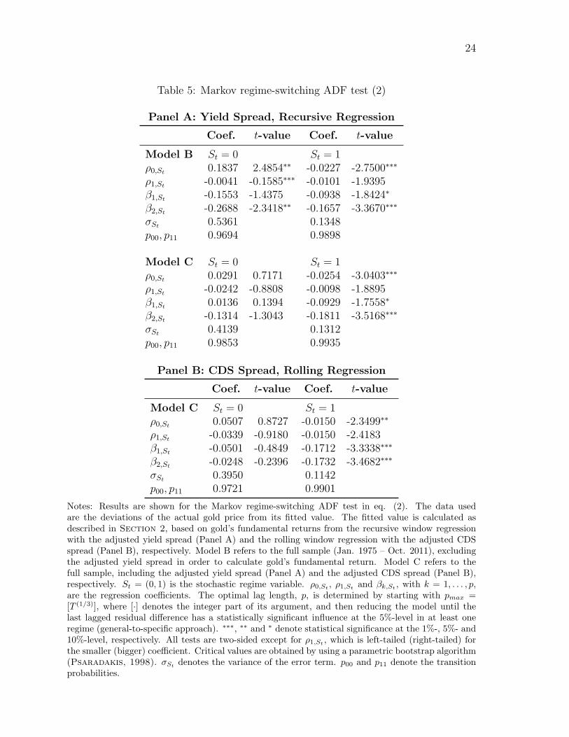
Finally, we re-run the Markov regime-switching ADF test from eq. (2), still using

the deviations of the actual gold price from its fitted value. Results for Models B and C

are reported in Panel A of Table 5. As in the case of the rolling window approach, we

see that the general-to-specific approach leads to model specifications with two lagged

differences. In addition, regime 0 is again more volatile, but less persistent than regime

1. However, also in the line with the results from Section 4.1, only Model B leads to

explosive deviations of the actual gold price from its fitted value, while Model C does

not indicate speculative bubbles. In short, we thus again conclude that the current

13

European sovereign debt crisis can be seen as the major reason for the current gold

price boom.


Apart from this check of the methodological robustness, we are also interested in

whether our results still hold if we draw on an alternative proxy for the current Euro-

pean sovereign debt crisis. Thus, we repeat the rolling window regression as outlined

in Section 4.2, but now use the (adjusted) spread between the 10-year senior credit

default swap (CDS) premium of Greece and Germany, instead of the yield spread, in

order to calculate gold’s fundamental returns. In a CDS on government bonds, the

protection buyer (e.g. a bank) purchases insurance against the event of default of the

security that the protection buyer holds. The buyer agrees with the protection seller

(e.g. an investor) to pay a premium. In the event of default, the protection seller has

to compensate the protection buyer for the loss incurred.

Descriptive statistics of the (adjusted) spread between the Greek and the German

CDS premium are reported in the last two rows of Panel A in Table 1. As in case

of the yield spread, the CDS spread was always positive but skyrocketed over the

last couple of years, reaching its peak of more than 37 percent in Oct. 2011. As a

consequence, it may serve as a reasonable alternative to the yield spread in order to

account for the current European sovereign debt crisis. Panel F of Figure 1 gives a

visual impression of the (original) CDS spread used for our empirical analysis.

In Panel C of Table 2, we show the results of the rolling window approach used

to calculate fitted gold returns. While the effects of the other fundamental factors are

similar to the results as reported in Panels A and B of Table 2, the adjusted CDS

spread has the expected positive influence on the gold return. Based on the fitted

gold returns, we again calculate gold’s fundamental value as outlined in Section 2,

and put it in relation to the actual gold price. Using the deviations of the actual gold

14

price from its fitted value, we then measure the stability of the ADF coefficient in the

conventional ADF equation. Results for Model C, with the yield spread replaced by

the CDS spread, are reported in Panel C of Table 3. As before, however, we do not

find different adjustment dynamics once we use the full sample and a proxy for the

current European sovereign debt crisis.

Finally, we again run the Markov regime-switching ADF test from eq. (2), still using

the deviations of the actual gold price from its fitted value. Results are reported in

Panel B of Table 5. As in the case of the yield spread, using the CDS spread in

Model C does not allow for finding speculative bubbles in the gold price. In short, we

thus again conclude that the current European sovereign debt crisis can be seen as the

major reason for the current gold price boom.

5. Conclusion

Motivated by the current gold price boom, this paper investigates whether rapidly

growing investment activities have caused a new asset price bubble. Drawing on gold’s

role as dollar hedge, inflation hedge, portfolio diversifier and safe haven, we calculate

fundamentally justified returns and approximate gold’s fundamental value. Based on

the deviations of the actual gold price from its fitted value, we then apply a Markov

regime-switching ADF test, which has substantial power to detect explosive behavior.

However, neither for the gold price boom from 1979 to 1982 nor in most recent times

can we find empirical evidence of speculative bubbles using this methodology.

The most likely explanation for our results is that three decades ago, skyrocketing

inflation (caused by the second oil crisis and amplified by a very expansive monetary

and fiscal policy) and geopolitical turmoil (especially due to the start of the Iran-Iraq

war and the Soviet invasion of Afghanistan) caused financial market participants to

look for stable investments in unstable times. Similarly, many investors have returned

to gold as a safe haven in these times of financial insecurity and the current European

sovereign debt crisis, thereby creating excess demand and the corresponding price surge.

15

References

Adrangi , B., Chatrath , A., Raffiee, K., 2003. Economic Activity, Inflation, and Hedg-

ing: The Case of Gold and Silver Investments. Journal of Wealth Management

6(2), 60-77.

Baur, D. G., Lucey, B. M., 2010. Is Gold a Hedge or a Safe Haven? An Analysis of

Stocks, Bonds and Gold. Financial Review 45(2), 217-229.

Baur, D. G., McDermott, T. K., 2010. Is Gold a Safe Haven? International Evidence.

Journal of Banking and Finance 34(8), 1886-1898.

Bertus, M., Stanhouse, B., 2001: Rational Speculative Bubbles in the Gold Futures

Market: Application of Dynamic Factor Analysis. Journal of Futures Markets

21(1), 79-108.

Blanchard, O. J., Watson, M. W., 1982: Bubbles, Rational Expectations and Financial

Markets. NBER Working Paper No. 945.

Blose, L. E., 2010. Gold Prices, Cost of Carry, and Expected Inflation. Journal of

Economics and Business 62(1), 35-47.

Capie, F., Mills, T. C., Wood, G., 2005: Gold as a Hedge against the Dollar. Journal

of International Financial Markets, Institutions and Money 15(4), 343-352.

Chan, K. F., Treepongkaruna, S., Brooks, R., Gray, S., 2011. Asset Market Linkages:

Evidence from Financial, Commodity and Real Estate Assets. Journal of Banking

and Finance 35(6), 1415-1426.

Diba, B. T., Grossman, H. I., 1984. Rational Bubbles in the Price of Gold. NBER

Working Paper No. 1300.

Evans, G. W., 1991. Pitfalls in Testing for Explosive Bubbles in Asset Prices. American

Economic Review 81(4), 922-930.

Funke, M., Hall, S. G., Sola, M., 1994. Rational Bubbles during Poland’s Hyperinfla-

tion – Implications and Empirical Evidence. European Economic Review 38(6),

1257-1276.

16

Gurkaynak, R. S., 2008. Econometric Tests of Asset Price Bubbles: Taking Stock.

Journal of Economic Surveys 22(1), 166-186.

Hall, S. G., Psaradakis, Z., Sola, M., 1999. Detecting Periodically Collapsing Bubbles:

A Markov-Switching Unit Root Test. Journal of Applied Econometrics 14(2),

143-154.

Hamilton, J. D., 1994. Time Series Analysis. Princeton, NJ: Princeton University

Press.

Hillier, D., Draper, P., Faff, R., 2006. Do Precious Metals Shine? An Investment

Perspective. Financial Analysts Journal 62(2), 98-106.

Homm, U., Breitung, J., 2011. Testing for Speculative Bubbles in Stock Markets: A

Comparison of Alternative Methods. Journal of Financial Econometrics, forth-

coming.

Jaffe, J. F., 1989. Gold and Gold Stocks as Investments for Institutional Portfolios.

Financial Analysts Journal 45(2), 53-59.

Kim, C. J., Nelson, C. R., 2000. State Space Models with Regime Switching. Cam-

bridge, MA: MIT Press.

Phillips, P. C. B., Yu, J., 2010. Dating the Timeline of Financial Bubbles during the

Sub-prime Crisis. Cowles Foundation Discussion Paper No. 1770.

Pindyck, R. S., 1993. The Present Value Model of Rational Commodity Pricing. Eco-

nomic Journal 103(418), 511-530.

Psaradakis, Z., 1998. Bootstrap-based Evaluation of Markov-Switching Time Series

Models. Econometric Reviews 17(3), 275-288.

Pukthuanthong, K., Roll, R., 2011. Gold and the Dollar (and the Euro, Pound, and

Yen). Journal of Banking and Finance 35(8), 2070-2083.

Shafiee, S., Topal, E. 2010. An Overview of Global Gold Market and Gold Price

Forecasting. Resources Policy 35(3), 178-189.

Sjaastad, L. A., Scacciavillani, F., 1996. The Price of Gold and the Exchange Rate.

Journal of International Money and Finance 15(6), 879-897.

17

Tully, E., Lucey, B. M., 2007. A Power GARCH Examination of the Gold Market.

Research in International Business and Finance 21(2), 316-325.

Went, P., Jirasakuldech, B., Emekter, R., 2009. Bubbles in Commodities Markets,

SSRN Working Paper.

World Gold Council, 2010. World Gold Council Publications Archive. www.gold.org.

Worthington, A.C., Pahlavani, M., 2007. Gold Investment as an Inflationary Hedge:

Cointegration Evidence with Allowance for Endogenous Structural Breaks. Ap-

plied Financial Economics Letters 3(4), 259-262.

18

Figure 1: Gold Return and Fundamental Factors

Notes: Panel A shows the change of the gold price (in US Dollars) per troy ounce (in percent). Panel B showsthe trade-weighted value of the US Dollar against other major currencies. Panel C shows the change of the USall-urban consumer price index (in percent). Panel D shows the change of the MSCI World index of major stockmarkets (in percent). Panel E shows the 3-month US Treasury bill rate (in percent). Panel F shows the spreadbetween Greece’s and Germany’s 10-year government bond yield (solid line) and between their 10-year seniorCDS premium (dashed line; in percent). All time series are given on a monthly frequency. Panels A to E coverthe full sample (Jan. 1975 – Oct. 2011). Panel F covers the shortened sample (Jan. 2003 – Oct. 2011).

‐30

‐20

‐10

0

10

20

30

1975 1980 1985 1990 1995 2000 2005 2010

Percen

t

Trade‐weighted Value of the US Dollar

60

70

80

90

100

110

120

130

140

150

1975 1980 1985 1990 1995 2000 2005 2010

Inde

x

Trade‐weighted Value of the US Dollar

‐4

‐2

0

2

4

6

8

10

12

14

16

1975 1980 1985 1990 1995 2000 2005 2010

Percen

t

US CPI Inflation Rate

‐25

‐20

‐15

‐10

‐5

0

5

10

15

20

1975 1980 1985 1990 1995 2000 2005 2010

Percen

tMSCI World Return

0

2

4

6

8

10

12

14

16

18

20

1975 1980 1985 1990 1995 2000 2005 2010

Percen

t

3‐Month US Treasury Bill Rate

0

5

10

15

20

25

30

35

40

0

2

4

6

8

10

12

14

16

18

2003 2004 2005 2006 2007 2008 2009 2010 2011

Percen

t

Percen

t

Yield Spread (left scale)

CDS Spread (right scale)

Panel A: Gold Return Panel B: Trade-weighted Value of the US Dollar

Panel C: US CPI Inflation Rate Panel D: MSCI World Return

Panel E: 3-Month US Treasury Bill Rate Panel F: 10-Year Bond Yield and CDS Spread

19

Figure 2: Gold Price, Fitted Value and Residual – Smoothed and Filter Probabilities Model B: Excluding Adj. Yield Spread Model C: Including Adj. Yield Spread

Notes: The left column refers to Model B which excludes the adjusted yield spread in order to calculate gold’sfundamental return. The right column refers to Model C which includes the adjusted yield spread. Both modelscover the full sample (Jan. 1975 – Oct. 2011). In both columns, the upper figure shows the actual gold price(solid line), its fitted value (dotted line) and the difference between both time series (dashed line). The fittedvalue is calculated as described in the text. All time series are denoted in US Dollars per troy ounce. The lowerfigure of each column shows the smoothed (solid line) and the filter probabilities (dotted line) of being in regime1, using the Markov regime-switching ADF test in eq. (2), which is based on the difference between the actualgold price and its fitted value.

‐500

0

500

1000

1500

2000

1975 1980 1985 1990 1995 2000 2005 2010

US‐Dollars per Troy Oun

ce

Gold Price, Fitted Value and Residual

Gold Price Fitted Gold Price Residual

‐500

0

500

1000

1500

2000

1975 1980 1985 1990 1995 2000 2005 2010US‐Dollars per Troy Oun

ce

Gold Price, Fitted Value and Residual

Gold Price Fitted Gold Price Residual

0.0

0.1

0.2

0.3

0.4

0.5

0.6

0.7

0.8

0.9

1.0

1975 1980 1985 1990 1995 2000 2005 2010

Prob

ability

Smoothed and Filter Probabilities

Smoothed Filter

0.0

0.1

0.2

0.3

0.4

0.5

0.6

0.7

0.8

0.9

1.0

1975 1980 1985 1990 1995 2000 2005 2010

Prob

ability

Smoothed and Filter Probabilities

Smoothed Filter

20

Table 1: Descriptive Statistics

Panel A: Univariate Time Series

Mean Max Min Stdev. Skew Kurt ADF

Gold 0.4936 25.2158 -23.6964 5.6013 0.1930 5.9699 I(0)Exchange Rate -0.0789 6.4662 -5.3910 1.7275 -0.0464 3.3963 I(0)Inflation 4.1071 13.6210 -2.0055 2.7823 1.4004 4.9086 I(1)Adj. Inflation -0.1116 3.2747 -4.1243 1.1806 -0.4361 3.5819 I(0)MSCI World 0.5882 13.5659 -20.8410 4.4837 -0.6567 5.1882 I(0)T-Bill 5.3720 15.5900 0.0200 3.2998 0.6517 3.6748 I(1)Adj. T-Bill -0.1131 4.6575 -4.5750 1.1583 -0.0228 5.1133 I(0)Yield Spread 2.3271 16.0400 0.1300 3.9174 2.0480 6.1687 I(1)Adj. Yield Spr. 0.7829 5.5208 -0.5941 1.5109 1.8203 5.0533 I(0)CDS Spread 2.2813 37.5272 0.0860 5.1040 4.2086 25.1844 I(1)Adj. CDS Spr. 1.0270 26.8701 -0.4150 3.1519 5.9306 45.4743 I(0)

Panel B: Correlation Analysis

Exchange Adj. MSCI Adj. Adj.Rate Inflation World T-Bill Yield Spr.

Exchange Rate 1.0000 -0.0105 -0.3898 -0.0272 0.1383Adj. Inflation -0.0825 1.0000 0.0232 0.0257 -0.1213MSCI World -0.1463 -0.0475 1.0000 0.2803 -0.3091Adj. T-Bill 0.0835 0.4591 -0.1083 1.0000 -0.2098Adj. Yield Spr. – – – – 1.0000

Notes: Panel A reports the arithmetic mean (Mean), the maximum (Max), the minimum (Min),the standard deviation (Stdev.), the skewness (Skew), the kurtosis (Kurt) and the degree of inte-gration based on the Augmented Dickey-Fuller test (ADF) for the change of the gold price per troyounce (Gold), the change of the trade-weighted value of the US Dollar against other major cur-rencies (Exchange Rate), the (adjusted) change of the US all-urban consumer price index ((Adj.)Inflation), the change of the MSCI index of major stock markets (MSCI World), the (adjusted)3-month US Treasury bill rate ((Adj.) T-Bill) and the (adjusted) spread between the 10-year gov-ernment bond yield of Greece and Germany ((Adj.) Yield Spr.). I(0) indicates stationarity andI(1) indicates a unit-root. Time series which contain a unit-root are adjusted by subtracting therespective variable’s mean of the previous year. All variables are calculated as continuous changesin percent and refer to the last day of a month, except for the (adjusted) US inflation rate whichis only available on a monthly frequency anyway. All time series consist of 442 observations (Jan.1975 – Oct. 2011), except for the (adjusted) yield spread which includes 106 observations (Jan.2003 – Oct. 2011). In Panel B, the lower triangular matrix reports the average correlations amongthe change of the effective US exchange rate, the adjusted US inflation rate, the world stock marketreturn and the adjusted 3-month US Treasury bill rate for the sample from Mar. 1975 to Dec. 2007(335 correlation matrices). The upper triangular matrix also includes the adjusted spread betweenthe 10-year government bond yield of Greece and Germany, and shows the average correlations forthe sample from Feb. 2003 to Oct. 2011 (46 correlation matrices). The correlation matrices arecalculated based on the method of Bravais-Pearson.

21

Table 2: Regression Results

Panel A: Yield Spread, Rolling Regression

γt γt−1 γt−2 Sum S(γt) S(γt−1) S(γt−2)

Exchange Rate -0.5116 -0.3006 0.3104 -0.5018 0.4409 0.1601 0.1548Adj. Inflation -0.1658 3.0170 -2.2264 0.6248 0.1207 0.1784 0.3464MSCI World 0.2261 0.0809 0.1202 0.4273 0.1522 0.1259 0.2020Adj. T-Bill -1.3720 1.3962 -0.4279 -0.4037 0.1286 0.1574 0.1181Adj. Yield Spr. 9.9197 -0.3131 -3.8037 5.8028 0.4042 0.0851 0.1063

Panel B: Yield Spread, Recursive Regression


Exchange Rate -0.5297 -0.4075 0.4072 -0.5300 0.9238 0.3963 0.3254Adj. Inflation -0.6946 4.3309 -2.3805 1.2558 0.1706 0.3648 0.7637MSCI World 0.3147 0.1365 0.0477 0.4990 0.2440 0.5800 0.1496Adj. T-Bill -0.6103 -0.0552 0.0934 -0.5720 0.0787 0.0656 0.0787Adj. Yield Spr. 7.3450 -1.4695 -2.4151 3.4604 0.3191 0.0425 0.0425

Panel C: CDS Spread, Rolling Regression


Exchange Rate -0.4952 -0.2956 0.3140 -0.4768 0.4356 0.1496 0.1863Adj. Inflation -0.1724 3.0413 -2.2581 0.6107 0.1417 0.1968 0.3517MSCI World 0.2233 0.0831 0.1197 0.4261 0.1522 0.1233 0.1653Adj. T-Bill -1.2357 1.1552 -0.3037 -0.3842 0.0997 0.1522 0.1076Adj. CDS Spr. 1.9424 -1.5342 -0.1202 0.5285 0.2127 0.1702 0.0851

Notes: In Panels A and B, results are shown for the rolling and the recursive regression, respectively,in eq. (1) of the change of the gold price per troy ounce on the change of the trade-weighted valueof the US Dollar against other major currencies (Exchange Rate), the adjusted change of theUS all-urban consumer price index (Adj. Inflation), the change of the MSCI index of major stockmarkets (MSCI World), the adjusted 3-month US Treasury bill rate (Adj. T-Bill) and the adjustedspread between the 10-year government bond yield of Greece and Germany (Adj. Yield Spr.). InPanel C, results are shown for the rolling regression in eq. (1) with the adjusted CDS spread(Adj. CDS Spr.) replacing the adjusted yield spread. γt, γt−1 and γt−2 are the mean values of thecontemporaneous (t) and the one- (t− 1) and two-period lagged (t− 2) influence, respectively, ofthe variables in the first column on the gold return based on the rolling regression (Panels A andC) and the recursive regression (Panel B), respectively. Sum is the mean aggregate impact of thecontemporaneous and the one- and two-period lagged regressors, respectively, on the gold return(γt + γt−1 + γt−2). S(γt), S(γt−1) and S(γt−2) are the number of significant parameters (at the10%-level) in relation to the total number of windows, which include the respective variable, for thecontemporaneous and the one- and two-period lagged influence, respectively, on the gold return.The mean value of the adjusted coefficient of determination is 0.1261 (Panel A), 0.1680 (Panel B)and 0.1283 (Panel C).

22

Table 3: Stability Tests

Panel A: Yield Spread, Rolling Regression

SupLR Prob. ExpLR Prob. AveLR Prob.

Model A 8.7632 0.0466 0.6745 0.3266 0.8642 0.4046Model B 19.4473 0.0003 8.1028 0.0000 13.0593 0.0000Model C 3.7317 0.4172 0.1437 0.9104 0.2387 0.8983

Panel B: Yield Spread, Recursive Regression


Model B 9.8708 0.0280 3.2438 0.0110 4.5945 0.0112Model C 3.9289 0.3855 0.3174 0.6213 0.4223 0.7142

Panel C: CDS Spread, Rolling Regression


Model C 3.4477 0.4667 0.0783 0.9999 0.1329 0.9993

Notes: Results are shown for Quandt-Andrews unknown breakpoint tests measuring the stabilityof the ADF coefficient in the conventional ADF equation. The data used are the deviations of theactual gold price from its fitted value. The fitted value is calculated as described in Section 2.Model A refers to the shortened sample (Jan. 1975 – Dec. 2007), excluding the adjusted yieldspread in order to calculate gold’s fundamental return. Model B refers to the full sample (Jan.1975 – Oct. 2011), again excluding the adjusted yield spread. Model C refers to the full sample,including the adjusted yield spread (Panels A and B) and the adjusted CDS spread (Panel C),respectively. SupLR, ExpLR and AveLR are the values of the supremum, the exponential and theaverage likelihood ratio test, respectively, and Prob. is the corresponding p-value. The optimallag length of the conventional ADF equation is determined by using the Schwartz informationcriterion.

23

Table 4: Markov regime-switching ADF test (1)

Yield Spread, Rolling Regression

Coef. t-value Coef. t-value

Model A St = 0 St = 1ρ0,St 0.2339 3.6081∗∗∗ -0.0186 -2.9499∗∗∗

ρ1,St -0.1234 -2.8328 -0.0175 -2.8594β1,St 0.0140 0.1171 -0.1958 -3.8432∗∗∗

β2,St -0.2380 -1.9490∗ -0.1891 -3.8080∗∗∗

σSt 0.3033 0.1111p00, p11 0.9318 0.9863

Model B St = 0 St = 1ρ0,St 0.1283 1.8731∗ -0.0167 -2.6275∗∗∗

ρ1,St 0.0298 1.3661∗∗∗ -0.0167 -2.7406β1,St -0.2395 -2.2438∗∗ -0.1811 -3.5993∗∗∗

β2,St -0.3598 -3.2281∗∗∗ -0.1725 -3.5626∗∗∗

σSt 0.4614 0.1138p00, p11 0.9700 0.9895

Model C St = 0 St = 1ρ0,St 0.0409 0.7690 -0.0165 -2.6001∗∗∗

ρ1,St -0.0288 -0.7949 -0.0161 -2.6170β1,St -0.0016 -0.0162 -0.1814 -3.5434∗∗∗

β2,St -0.1259 -1.1924 -0.1803 -3.6233∗∗∗

σSt 0.4109 0.1133p00, p11 0.9717 0.9898

Notes: Results are shown for the Markov regime-switching ADF test in eq. (2). The data used are thedeviations of the actual gold price from its fitted value. The fitted value is calculated as described inSection 2. Model A refers to the shortened sample (Jan. 1975 – Dec. 2007), excluding the adjustedyield spread in order to calculate gold’s fundamental return. Model B refers to the full sample (Jan.1975 – Oct. 2011), again excluding the adjusted yield spread. Model C refers to the full sample,including the adjusted yield spread. St = (0, 1) is the stochastic regime variable. ρ0,St , ρ1,St andβk,St , with k = 1, . . . , p, are the regression coefficients. The optimal lag length, p, is determined bystarting with pmax = [T (1/3)], where [·] denotes the integer part of its argument, and then reducing themodel until the last lagged residual difference has a statistically significant influence at the 5%-levelin at least one regime (general-to-specific approach). ∗∗∗, ∗∗ and ∗ denote statistical significance atthe 1%-, 5%- and 10%-level, respectively. All tests are two-sided except for ρ1,St , which is left-tailed(right-tailed) for the smaller (bigger) coefficient. Critical values are obtained by using a parametricbootstrap algorithm (Psaradakis, 1998). σSt

denotes the variance of the error term. p00 and p11

denote the transition probabilities.

24

Table 5: Markov regime-switching ADF test (2)

Panel A: Yield Spread, Recursive Regression


Model B St = 0 St = 1ρ0,St 0.1837 2.4854∗∗ -0.0227 -2.7500∗∗∗

ρ1,St -0.0041 -0.1585∗∗∗ -0.0101 -1.9395β1,St -0.1553 -1.4375 -0.0938 -1.8424∗

β2,St -0.2688 -2.3418∗∗ -0.1657 -3.3670∗∗∗

σSt 0.5361 0.1348p00, p11 0.9694 0.9898

Model C St = 0 St = 1ρ0,St 0.0291 0.7171 -0.0254 -3.0403∗∗∗

ρ1,St -0.0242 -0.8808 -0.0098 -1.8895β1,St 0.0136 0.1394 -0.0929 -1.7558∗

β2,St -0.1314 -1.3043 -0.1811 -3.5168∗∗∗

σSt 0.4139 0.1312p00, p11 0.9853 0.9935

Panel B: CDS Spread, Rolling Regression


Model C St = 0 St = 1ρ0,St 0.0507 0.8727 -0.0150 -2.3499∗∗

ρ1,St -0.0339 -0.9180 -0.0150 -2.4183β1,St -0.0501 -0.4849 -0.1712 -3.3338∗∗∗

β2,St -0.0248 -0.2396 -0.1732 -3.4682∗∗∗

σSt 0.3950 0.1142p00, p11 0.9721 0.9901

Notes: Results are shown for the Markov regime-switching ADF test in eq. (2). The data usedare the deviations of the actual gold price from its fitted value. The fitted value is calculated asdescribed in Section 2, based on gold’s fundamental returns from the recursive window regressionwith the adjusted yield spread (Panel A) and the rolling window regression with the adjusted CDSspread (Panel B), respectively. Model B refers to the full sample (Jan. 1975 – Oct. 2011), excludingthe adjusted yield spread in order to calculate gold’s fundamental return. Model C refers to thefull sample, including the adjusted yield spread (Panel A) and the adjusted CDS spread (Panel B),respectively. St = (0, 1) is the stochastic regime variable. ρ0,St

, ρ1,Stand βk,St

, with k = 1, . . . , p,are the regression coefficients. The optimal lag length, p, is determined by starting with pmax =[T (1/3)], where [·] denotes the integer part of its argument, and then reducing the model until thelast lagged residual difference has a statistically significant influence at the 5%-level in at least oneregime (general-to-specific approach). ∗∗∗, ∗∗ and ∗ denote statistical significance at the 1%-, 5%- and10%-level, respectively. All tests are two-sided except for ρ1,St

, which is left-tailed (right-tailed) forthe smaller (bigger) coefficient. Critical values are obtained by using a parametric bootstrap algorithm(Psaradakis, 1998). σSt

denotes the variance of the error term. p00 and p11 denote the transitionprobabilities.

Documents

Is There a Speculative Bubble in the Price of Gold