Isentropic Analysis of Polar Cold Airmass Streams in the Northern Hemispheric Winter

TOSHIKI IWASAKI, TAKAMICHI SHOJI, AND YUKI KANNO

Graduate School of Science, Tohoku University, Sendai, Japan

MASAHIRO SAWADA

Atmosphere and Ocean Research Institute, University of Tokyo, Tokyo, Japan

MASASHI UJIIE

Japan Meteorological Agency, Tokyo, Japan

KOUTAROU TAKAYA

Research Institute for Global Change, JAMSTEC, Yokohama, Japan

(Manuscript received 15 February 2013, in final form 15 February 2014)

ABSTRACT

An analysis method is proposed for polar cold airmass streams from generation to disappearance. It des-

ignates a threshold potential temperature uT at around the turning point of the extratropical direct (ETD)

meridional circulation from downward to equatorward in the mass-weighted isentropic zonal mean (MIM)

and clarifies the geographical distributions of the cold air mass, the negative heat content (NHC), their

horizontal fluxes, and their diabatic change rates on the basis of conservation relations of the air mass and

thermodynamic energy. In the Northern Hemispheric winter, the polar cold air mass below uT 5 280K has

two main streams: the East Asian stream and the North American stream. The former grows over the

northern part of the Eurasian continent, flows eastward, turns down southeastward toward East Asia via

Siberia, and disappears over the western North Pacific Ocean. The latter grows over the Arctic Ocean, flows

toward the eastern coast of North America via Hudson Bay, and disappears over the western North Atlantic

Ocean. In their exit regions, wave–mean flow interactions are considered to transfer the angular momentum

from the cold airstreams to the upward Eliassen–Palm flux and convert the available potential energy to wave

energy.

1. Introduction

The zonal mean meridional circulation diagnosed

with mass-weighted isentropic zonal means (MIM) ex-

hibits a distinct extratropical direct (ETD) circulation in

winter hemispheres (Townsend and Johnson 1985;

Johnson 1989; Iwasaki 1989, 1992; Juckes et al. 1994;

Juckes 2001). InMIM, themass streamfunctions are free

from the Stokes drift, and indicate Lagrangian mean-

meridional circulations (e.g., Iwasaki 1989). The zonal

mean thermodynamic equation, which does not have

any eddy terms, provides a simple physical insight of

heat transport. In midlatitudes, the ETD circulation was

shown to conduct considerable poleward heat transport

(e.g., Czaja and Marshall 2006). In the lower tropo-

sphere, the cold air mass generated in the polar region

outflows equatorward and cools down the subtropical

atmosphere (Iwasaki and Mochizuki 2012, hereinafter

IM12). Such a simple view is based on the zonally in-

tegrated meridional circulation on isentropic surfaces.

The actual geographical distributions of equatorward

flow may be under a great influence of the topography

and the land–sea thermal contrast. Our increasing in-

terest is in the geographical routing of the cold airmass

stream from the polar region to lower latitudes from the

viewpoint of isentropic airmass circulations.

What is the driving force of the low-level cold airmass

streams equatorward? The angular momentum balance

is essential to the formation of the low-level equatorward

Corresponding author address: Toshiki Iwasaki, Graduate

School of Science, Tohoku University, Aoba-ku, Sendai 980-8578,

Japan.

E-mail: iwasaki@wind.gp.tohoku.ac.jp

2230 JOURNAL OF THE ATMOSPHER IC SC IENCES VOLUME 71

DOI: 10.1175/JAS-D-13-058.1

� 2014 American Meteorological Society

flow. In the MIM’s zonal mean, the lower-tropospheric

equatorward flow is driven through wave–mean flow in-

teractions (e.g., IM12). The Coriolis force of the equa-

torward flow is almost in balance with Eliassen–Palm

(E–P) flux divergence (Juckes et al. 1994; Tanaka et al.

2004; IM12). It indicates that long and ultralong waves

play important roles in the formation of the equator-

ward flow. This is somewhat similar to the extratropical

pumping, which is well known as a major driving force

of the stratospheric mean meridional circulation (e.g.,

Holton et al. 1995). In this work, the idea of the ex-

tratropical pumping is extended to the localized cold

stream in the lower troposphere, with particular at-

tention on the lower boundary conditions.

Many studies have been done on the polar cold air

outbreaks frequently causing extreme cold events in

mid- and low latitudes, especially around eastern North

America (e.g., Dallavalle and Bosart 1975) and East

Asia (e.g., Chang et al. 1979). Intermittent cold air

outbreaks are accompanied by synoptic traveling dis-

turbances in midlatitudes (e.g., Joung and Hitchman

1982; Lau and Lau 1984). The geographical features

of outbreaks are associated with the downstream de-

velopment of synoptic disturbances from high moun-

tains under control of quasi-stationary ultralong waves.

The activity of quasi-stationary ultralong waves induces

intraseasonal and interannual variations of cold air

outbreaks (e.g., Boyle 1986; Schultz et al. 1998; Takaya

and Nakamura 2005; Jeong and Ho 2005; Park et al.

2011). In isobaric coordinates, however, the time-mean

wind hardly indicates the cold airmass flux, because it

includes warm winds. Therefore, previous studies

treated the cold air outbreaks as anomalous events de-

viated from the normal climate. Direct estimates, how-

ever, have not been made of the stationary component

of polar cold airmass flux yet.

Isentropic coordinates are convenient to trace the

airmass trajectory. Harada (1962) studied the rapid ad-

vancement of the head of cold air outbreak around Ja-

pan in isentropic coordinates. Most isentropic analyses

dealt with single-level synoptic charts subjectively, but

did not deal with mass and heat balances quantitatively.

The mass weighting introduced toMIM leads us to simple

expressions of conservations of air mass and thermody-

namic energy. The purpose of this study is to develop

a quantitative diagnosis tool for the geographical distri-

butions of polar cold airstreams in isentropic coordinates,

which estimates its genesis/loss rates of a cold air mass

based on conservations of the cold air mass and the neg-

ative heat content. A preliminary analysis is made on the

Northern Hemispheric winter climate of the polar cold

airstreams, negative heat flows, and their diabatic genesis/

loss. Particular attention is paid to the stationary component

of polar cold airmass streams. Data used are the atmo-

spheric reanalysis from the Japanese 25-year Reanalysis

Project (JRA-25), conducted at the Japan Meteorolog-

ical Agency (Onogi et al. 2007).

2. Conservation relations of polar cold air massand negative heat content

In this analysis, one of the key parameters in identi-

fying the polar cold air mass is the threshold potential

temperature uT . In MIM analyses, the potential tem-

perature at the turning point of the ETD circulation

from the downward to the equatorward seems to be

appropriate as a threshold value of the polar cold air

mass, because the downward motion indicates the for-

mation of the cold air mass and the equatorward motion

reduces temperature owing to the horizontal advection

in isentropic coordinates (IM12). Of course, the choice

of uT is still open and impacts of modified thresh-

old temperatures will be discussed in section 5.

We first derive the governing equation of geo-

graphical distribution of the cold air mass below the

threshold potential temperature. Symbols are listed in

appendix B. At each grid point on the sphere, the total

cold airmass amount below uT is given by the pressure

difference between the ground surface and the isentro-

pic surface of uT ,

DP[ pS 2 p(uT) . (1)

The isentropic mass continuity equation (see, e.g.,

Johnson 1980) can be written as

›

›t

�›p

›u

�1$ �

�›p

›uv

�1

›

›u

�›p

›u_u

�5 0. (2)

The vertical integration of Eq. (2) from the lower

boundary us to uT leads us to the total cold airmass

conservation equation

›

›tDP52$ �

ðps

p(uT)

vdp1G(uT) . (3)

The total cold airmass amount changes as a result of

horizontal convergence and the vertical mass flux at uT .

The vertical mass flux crossing the uT surface G(uT) is

related to the diabatic heating/cooling at uT ,

G(uT)[›p

›u_u

����uT

, (4)

where the diabatic cooling is the source of the cold air

mass. Here G(uT) becomes negative when the cold air

JUNE 2014 IWASAK I ET AL . 2231

mass disappears because of diabatic heating. For longer

periods, Eq. (3) is reduced to the balance between the

horizontal cold airmass flux divergence and the diabatic

change in the cold air mass,

$ �" ðp

s

p(uT)

v dp

#’ [G(uT)] , (5)

where the square brackets here indicate time means.

The simple relationship can be derived on the basis of

constant threshold potential temperature. An important

difference from isobaric coordinates is that the vertical

mass flux G(uT) is evaluated on an isentropic surface of

uT . If the mass flux is evaluated on an isobaric surface,

the vertical mass flux is dominated by adiabatic vertical

motions and the horizontal airmass flux may be subject

to the Stokes drifts. In the isentropic analysis, source/

sink of horizontal flux is limited to diabatic changes, and

its steady state suggests the Lagrangian mean mass flux.

The cold airmass amount does not consider potential

temperature the surface. To measure the strength of

coldness, let us define negative heat content (NHC)

below uT as an alternative thermodynamic parameter,

which reflects vertical profiles of air temperature,

q(uT)[

ðps

p(uT)

(uT 2 u) dp . (6)

The NHC is proportional to the product of air mass

pS 2p(uT) and vertically averaged potential tempera-

ture difference uT 2 u below uT , as is shown by the

hatched area in Fig. 1. The governing equation is derived

as follows. Multiplying Eq. (2) by u leads us to

›

›t

�u›p

›u

�1$ �

�u›p

›uv

�1

›

›u

�u›p

›u_u

�2

›p

›u_u5 0. (7)

Again, multiply Eq. (2) by uT and subtract Eq. (7) from

it, and we have

›

›t(uT 2 u)

›p

›u1$ � (uT 2 u)

›p

›uv

1›

›u

�(uT 2 u)

›p

›u_u

�1

›p

›u_u5 0.

The vertical integration from us to uT yields

›

›tq52$ �

ðps

p(uT)

(uT 2 u)vdp2

ðps

p(uT)

_u dp . (8)

Thus, the NHC can be handled as a conservative ther-

modynamic budget. Note that no vertical heat flux in the

third term on the left-hand side of Eq. (7) contributes to

the NHC, since the negative heat (uT 2 u) is zero at uT .

The diabatic cooling/heating in the interior region below

uT contributes to the NHC genesis/loss, respectively.

Averaging over longer periods, the tendency in Eq. (8) is

relatively small, so that we have

$ �" ðp

s

p(uT)

(uT 2 u)v dp

#’2

" ðps

p(uT)

_udp

#, (9)

where again, the square brackets indicate time means.

The NHC flux divergence is almost in balance with the

diabatic cooling.

Numerical computations are made of the cold airmass

amount, its horizontal flux, the NHC, and its horizontal

flux on the basis of the above formulations from the

reanalysis JRA-25 (Onogi et al. 2007). Data at manda-

tory pressure levels of JRA-25 are vertically integrated

with respect to pressure from the level of uT to the

surface every 6 h. Results are subject to numerical errors

and the accuracy depends on the vertical resolutions of

mandatory levels in the lower troposphere. The diabatic

changes in the cold air mass and the NHC are estimated

from its flux convergences as the residuals of conserva-

tion relations [Eqs. (3) and (8)].

3. Isentropic analysis of polar cold air mass

a. Threshold potential temperature for the polarcold air mass

First, we designate the threshold potential temper-

ature for the polar cold air mass. Figure 2 illustrates

MIM’s mass streamfunctions (e.g., Iwasaki 1989; IM12)

together with potential temperature for isentropic zonal

mean pressures in December–February (DJF), averag-

ing over 30 winters from 1980/81 to 2009/2010. There we

find an extratropical direct circulation on the polar side

of Hadley circulation in the Northern Hemispheric

winter. The ETD circulation turns from downward to

FIG. 1. Schematic diagram of the cold airmass amount (pressure

difference) and negative heat content (NHC; hatched area). The

thick solid line indicates vertical profile of potential temperature.

2232 JOURNAL OF THE ATMOSPHER IC SC IENCES VOLUME 71

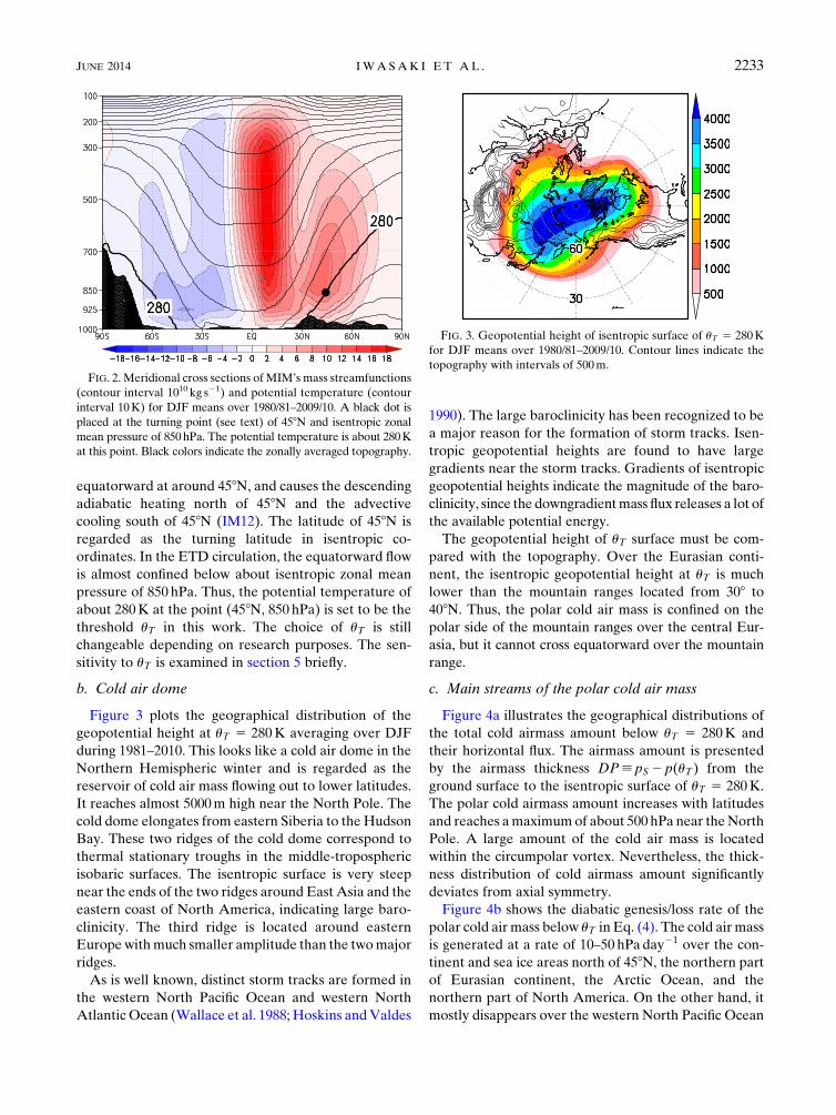
equatorward at around 458N, and causes the descending

adiabatic heating north of 458N and the advective

cooling south of 458N (IM12). The latitude of 458N is

regarded as the turning latitude in isentropic co-

ordinates. In the ETD circulation, the equatorward flow

is almost confined below about isentropic zonal mean

pressure of 850 hPa. Thus, the potential temperature of

about 280K at the point (458N, 850 hPa) is set to be the

threshold uT in this work. The choice of uT is still

changeable depending on research purposes. The sen-

sitivity to uT is examined in section 5 briefly.

b. Cold air dome

Figure 3 plots the geographical distribution of the

geopotential height at uT 5 280K averaging over DJF

during 1981–2010. This looks like a cold air dome in the

Northern Hemispheric winter and is regarded as the

reservoir of cold air mass flowing out to lower latitudes.

It reaches almost 5000m high near the North Pole. The

cold dome elongates from eastern Siberia to the Hudson

Bay. These two ridges of the cold dome correspond to

thermal stationary troughs in the middle-tropospheric

isobaric surfaces. The isentropic surface is very steep

near the ends of the two ridges around East Asia and the

eastern coast of North America, indicating large baro-

clinicity. The third ridge is located around eastern

Europewithmuch smaller amplitude than the twomajor

ridges.

As is well known, distinct storm tracks are formed in

the western North Pacific Ocean and western North

AtlanticOcean (Wallace et al. 1988; Hoskins andValdes

1990). The large baroclinicity has been recognized to be

a major reason for the formation of storm tracks. Isen-

tropic geopotential heights are found to have large

gradients near the storm tracks. Gradients of isentropic

geopotential heights indicate the magnitude of the baro-

clinicity, since the downgradientmass flux releases a lot of

the available potential energy.

The geopotential height of uT surface must be com-

pared with the topography. Over the Eurasian conti-

nent, the isentropic geopotential height at uT is much

lower than the mountain ranges located from 308 to

408N. Thus, the polar cold air mass is confined on the

polar side of the mountain ranges over the central Eur-

asia, but it cannot cross equatorward over the mountain

range.

c. Main streams of the polar cold air mass

Figure 4a illustrates the geographical distributions of

the total cold airmass amount below uT 5 280K and

their horizontal flux. The airmass amount is presented

by the airmass thickness DP[ pS 2 p(uT) from the

ground surface to the isentropic surface of uT 5 280K.

The polar cold airmass amount increases with latitudes

and reaches amaximumof about 500 hPa near theNorth

Pole. A large amount of the cold air mass is located

within the circumpolar vortex. Nevertheless, the thick-

ness distribution of cold airmass amount significantly

deviates from axial symmetry.

Figure 4b shows the diabatic genesis/loss rate of the

polar cold air mass below uT in Eq. (4). The cold air mass

is generated at a rate of 10–50 hPa day21 over the con-

tinent and sea ice areas north of 458N, the northern part

of Eurasian continent, the Arctic Ocean, and the

northern part of North America. On the other hand, it

mostly disappears over the western North Pacific Ocean

FIG. 2. Meridional cross sections of MIM’s mass streamfunctions

(contour interval 1010 kg s21) and potential temperature (contour

interval 10K) for DJF means over 1980/81–2009/10. A black dot is

placed at the turning point (see text) of 458N and isentropic zonal

mean pressure of 850hPa. The potential temperature is about 280K

at this point. Black colors indicate the zonally averaged topography.

FIG. 3. Geopotential height of isentropic surface of uT 5 280K

for DJF means over 1980/81–2009/10. Contour lines indicate the

topography with intervals of 500m.

JUNE 2014 IWASAK I ET AL . 2233

and the western North Atlantic Ocean. Both disap-

pearance regions have sharp line structures rising from

308N at the coasts to higher latitudes at their eastern

ends. This reflects the sea surface temperature (SST)

under a possible influence of the western boundary

currents and their extensions. The cold air mass rapidly

disappears at a maximal rate of about 100 hPa day21

owing to strong diabatic heating soon after it crosses

a line of the SST of 280K southward. Particularly in the

Atlantic Ocean, the loss region of cold air mass reaches

around 608N, where the Gulf Stream transports a large

amount of ocean heat content northward and releases it

to the atmosphere in higher latitudes (Minobe et al.

2008).

The mass flux can be decomposed into divergent/

irrotational and rotational/nondivergent components, as

shown in Figs. 4c and 4d,

[pv][

ðps

p(uT)

vdp5 [pv]x 1 [pv]c , (10)

where the divergent and rotational components can be

written in terms of scalar functions and the vertical unit

vector k,

[pv]x 5$x and [pv]c 52k3$c . (11)

The rotational component may present perpetual mo-

tions that are not directly related to the diabatic change

in the cold air mass. The divergent component primarily

explains the temporal change in the geographical dis-

tribution of the cold airmass amount as is expected from

Eq. (3). Note that only the divergent component con-

tributes to the mean meridional circulation in MIM as

shown in Fig. 2. Roughly speaking, the magnitude of

FIG. 4. Geographical distributions of (a) cold airmass amount (hPa) and its horizontal flux with arrows, (b) genesis/

loss of cold air mass (hPaday21) with the SST line of 280K, (c) divergent/irrotational component of cold airmass flux

(hPam s21), and (d) rotational/nondivergent component of cold airmass flux for DJF means over 1980/81–2009/10.

Contour lines indicate topography with intervals of 500m.

2234 JOURNAL OF THE ATMOSPHER IC SC IENCES VOLUME 71

divergent component is as large as that of rotational

component. The meridional cold airmass flux is domi-

nated by the divergent component, as shown in Fig. 4c.

In particular, the divergent component has the distinct

meridional cold airmass flux over East Asia and the

eastern coast of North America. On the other hand, the

circumpolar cold airmass flux is dominated by the ro-

tational component, especially over the northern part of

the Eurasian continent.

Figure 5 is similar to Fig. 4a, except for contouring the

magnitude of the cold airmass flux instead of the cold

airmass amount. Mass-weighted isentropic time-mean

mass flux suggests that the Lagrangian mean mass

transport is directly related to the diabatic genesis/loss.

The polar cold air mass is found to have two main

streams of the polar cold air mass. One main stream is

called ‘‘the East Asian (EA) cold stream.’’ The EA

stream grows over the northern part of the Eurasian

continent, flows eastward, turns southeastward around

Siberia, and gradually disappears over the western

North Pacific Ocean. Another is called ‘‘the North

American (NA) cold stream,’’ which grows because of

diabatic genesis over the Arctic Ocean, flows toward the

eastern coast of North America, and disappears over the

eastern North Atlantic Ocean. Within the polar vortex,

the flow field is changeable year by year and sometimes

the two main streams are difficult to separate.

Near the exit of the EA stream, cold surges occur

frequently (e.g., Zhang et al. 1997; Compo et al. 1999).

The exit of NA stream, the eastern coast of North

America, is also known as a region where cold surges

occur (e.g., Dallavalle and Bosart 1975). It suggests that

intermittent cold surges significantly contribute to the

climatic feature of the polar cold airmass streams.

In this work, the two main streams identified in the

climatological mean states are consistent with pathways

of intermittent cold surges reported in many previous

works (e.g., Dallavalle and Bosart 1975; Chang et al.

1979; Joung and Hitchman 1982; Lau and Lau 1984).

The routing of the main streams can be seen as follows:

In the case of the EA stream, the cold air mass originates

because of the diabatic cooling over the Eurasian con-

tinent. High mountain ranges in central Asia may act as

a barrier for the cold air mass to take lower positions,

and westerlies blow the cold air mass eastward on the

northern side of mountains. In East Asia, the cold air-

stream turns equatorward following the geostrophic

balance with the eastward pressure gradient forces

between the Siberian high and Aleutian low. The NA

stream is generated over the Arctic Ocean, steered

by the Rocky Mountains and Greenland, and geo-

strophically introduced toward the East Coast by the

Icelandic low. Both main streams have their major exits

over oceans and disappear just on the equatorial side of

the SST 5 280K line. In the case of uT 5 280K, disap-

pearance regions are near the storm tracks (Wallace

et al. 1988; Hoskins and Valdes 1990). Baroclinic in-

stability waves accompany equatorward cold airmass

flows on the western side of cyclonic centers (e.g.,

Iwasaki 1990). Thus, in a statistical sense, synoptic

disturbances are considered to contribute to the time-

mean equatorward cold airmass flux both over the

western North Pacific Ocean and western North At-

lantic Ocean.

d. Negative heat content

Negative heat content (NHC), which is the conser-

vative thermodynamic quantity for adiabatic processes,

is defined to directly measure the strength of ‘‘cold

waves.’’ According to Eq. (8), the NHC is generated

(lost) by dibatic cooling (heating) at all levels below uTand significantly affected by the surface diabatic heating.

This stands in contrast with the cold airmass amount

changed by diabatic cooling/heating only near the level

of u5 uT . In isobaric coordinates, the mean mass flux

sometime takes a significantly different direction from

mean heat flux because of the eddy correlations between

the temperature andmeridional wind. Thus, we examine

the similarity and difference of the NHC from the cold

airmass amount.

Figures 6a and 6b show geographical distributions of

the NHC with its horizontal flux and NHC generation

rates. In a qualitative sense, their geographical patterns

look similar to those of the cold airmass amount. Com-

pared with the cold airmass amount, the NHC elongates

more between East Asia and the U.S. East Coast. This is

closely related to temperature near the surface, which is

lower over the eastern Eurasia than over the western

Eurasia. The generation rate of theNHChas amuchmore

FIG. 5. As in Fig. 4, but for shading the magnitude of the cold

airmass flux (hPam s21). Contour lines indicate the topography

with intervals of 500m.

JUNE 2014 IWASAK I ET AL . 2235

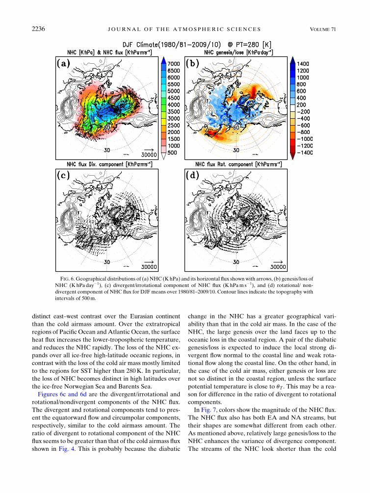
distinct east–west contrast over the Eurasian continent

than the cold airmass amount. Over the extratropical

regions of PacificOcean andAtlantic Ocean, the surface

heat flux increases the lower-tropospheric temperature,

and reduces the NHC rapidly. The loss of the NHC ex-

pands over all ice-free high-latitude oceanic regions, in

contrast with the loss of the cold air mass mostly limited

to the regions for SST higher than 280K. In particular,

the loss of NHC becomes distinct in high latitudes over

the ice-free Norwegian Sea and Barents Sea.

Figures 6c and 6d are the divergent/irrotational and

rotational/nondivergent components of the NHC flux.

The divergent and rotational components tend to pres-

ent the equatorward flow and circumpolar components,

respectively, similar to the cold airmass amount. The

ratio of divergent to rotational component of the NHC

flux seems to be greater than that of the cold airmass flux

shown in Fig. 4. This is probably because the diabatic

change in the NHC has a greater geographical vari-

ability than that in the cold air mass. In the case of the

NHC, the large genesis over the land faces up to the

oceanic loss in the coastal region. A pair of the diabatic

genesis/loss is expected to induce the local strong di-

vergent flow normal to the coastal line and weak rota-

tional flow along the coastal line. On the other hand, in

the case of the cold air mass, either genesis or loss are

not so distinct in the coastal region, unless the surface

potential temperature is close to uT . This may be a rea-

son for difference in the ratio of divergent to rotational

components.

In Fig. 7, colors show the magnitude of the NHC flux.

The NHC flux also has both EA and NA streams, but

their shapes are somewhat different from each other.

As mentioned above, relatively large genesis/loss to the

NHC enhances the variance of divergence component.

The streams of the NHC look shorter than the cold

FIG. 6. Geographical distributions of (a) NHC (KhPa) and its horizontal flux shownwith arrows, (b) genesis/loss of

NHC (KhPaday21), (c) divergent/irrotational component of NHC flux (KhPam s21), and (d) rotational/ non-

divergent component of NHC flux for DJF means over 1980/81–2009/10. Contour lines indicate the topography with

intervals of 500m.

2236 JOURNAL OF THE ATMOSPHER IC SC IENCES VOLUME 71

airmass streams. This is probably because the NHC de-

creases owing to the surface heat flux quickly when the

cold air mass moving from the land to the ocean. The

similarity between the cold mass flux and the NHC flux

suggests that the behavior of cold waves can be consid-

ered on the basis of the polar cold airmass flux. This may

be the great advantage of isentropic coordinates.

4. Angular momentum balance and energyconversion in the cold streams

The strong Coriolis force is exerted on the cold

airmass stream, and accelerates the equatorward flow

westward. The cold stream cannot go straight equator-

ward without eastward counter force to the Coriolis

force. In the mass-weighted isentropic zonal means

(MIM), the equatorward mass flow was shown to bal-

ance with the vertical E–P flux divergence at 458Nthrough the extratropical pumping in the context of

wave–mean flow interaction (IM12). In this case, the

angular momentum is transferred from the equatorward

flow to the upward E–P flux. Thus, we carefully look at

the local structure of E–P flux divergence in the vicinity

of the lower boundary.

Let us consider a typical case of the cold airmass

stream isolated by the isentropic line F(x, uT) and

the ground surface line FS(x) in a zonal plane, as

shown in Fig. 8. The ground surface geopotential height

and isentropic geopotential height of uT are further as-

sumed to be a monotonic function of longitudinal dis-

tance x, ›FS/›x# 0, (›F/›x)uT . 0 in region I, and

(›F/›x)uT , 0 in region II. This includes a special case of

a flat ground as FS(x2)5 0. Integrated over the domain,

the zonal momentum equation can be derived from

Eq. (A6) into

›

›thui5

ðFmax

0

(ðxII(F)

xI(F)

fry dx1 [pI(F)2 pII(F)]

)dF

2›

›yhuyi2

ðx2

x1

u _u›p

›udx1 hFxi .

(12)

Angle brackets indicate aerial integrations over the cold

air mass at a chosen latitude. The first term is the Cori-

olis force exerted on the cold airmass flux and the

pressure difference between pI(F) at the western edge

and pII(F) at the eastern edge of the cold air mass. The

pressure difference term is rewritten from the local

contribution to vertical divergence of E–P flux in isen-

tropic coordinates.

In the EA stream, we examine the time-mean vertical

profiles of the westward Coriolis forces exerted on the

southward component of the cold airmass flux and the

pressure difference between the western and eastern

edges of the cold air mass. The snapshot values of these

terms are so noisy that we evaluate time-mean pressure

and mass-weighted meridional wind velocity at some

isentropic surfaces, and convert them into the mean

meridional wind at geometric heights at each grid point.

The pressure difference pI(F)2 pII(F) is vertically in-

tegrated from the ground surface to uT . The westward

Coriolis force of the equatorward cold airmass flow is

balanced geostrophically with the pressure difference

between western and eastern edges, as shown in Fig. 9.

In the EA stream, the stationary eastward pressure

gradient force forms between the Siberian high and

Aleutian low and causes the equatorward cold airmass

flow. This is regarded as a local structure of quasi-

stationary ultralong waves. Also, baroclinic instability

waves accompany both of equatorward cold airstreams

and eastward pressure gradients behind of cyclonic

centers (Iwasaki 1990). As a result, baroclinic instability

FIG. 7. As in Fig. 6a, but for shading the magnitude of the flux

vector. Contour lines indicate the topography with intervals

of 500m.

FIG. 8. Schematic diagram of zonal component of pressure ex-

erted on the cold airmass stream. The mountain is heavily shaded

and the cold air mass below uT is lightly shaded. Western and

eastern edges of cold airstream are denoted as x1 and x2, re-

spectively. Isentropic geopotential height of uT is maximal at xmax,

and regions I and II indicate western and eastern sides of xmax. This

is the simple case that the surface geopotential height is a mono-

tonic function of x. Open arrows indicate pressures from the

ground or the upper atmosphere with higher potential temperature

to the cold air mass.

JUNE 2014 IWASAK I ET AL . 2237

waves may enhance the equatorward cold airmass flux

and the diabatic loss rate over the warm SST near the

storm track. Note that Eq. (12) includes the effects of

surface frictional andmountain torques, which exchange

the angular momentum between the atmosphere and

Earth. In the extratropics, the surface frictional and

mountain torques are expected to induce the poleward

flow near the lower boundary. However, it is inferior to

the equatorward flow driven by the E–P flux divergence

in MIM. This is consistent with the pioneering work in

MIM by Johnson (1989) that the pressure torque is

dominant in the extratropical lower troposphere.

The eastward pressure gradient force on longitudi-

nally isolated cold air mass by an isentropic line not only

induces net equatorward flow geostrophically, but also

generates the upward E–P flux. The cold air mass

presses the upper-isentropic surface and the lower

ground surface westward, as the reaction to the eastward

pressure gradient force from the surrounding air mass

and the ground surface. Thus, the regions of stationary

eastward pressure gradient force and the storm track

become local sources of upward flux of westward an-

gular momentum (Egger and Hoinka 2010). In this

process, the westward angular momentum is transferred

from the equatorward cold airmass stream to the ver-

tical E–P flux. The E–P flux propagates upward and

converges in the upper troposphere. The deceleration of

westerly flow due to wave–mean flow interactions drives

the mean poleward flow through the so-called extra-

tropical pumping in the upper troposphere.

The energetics is also an important viewpoint of

wave–mean flow interactions. In theMIM analysis, their

energetics is understood in terms of the cascade-type

conversions from the available potential energy AZ to

the wave energy W 5 AE 1 KE, via the zonal mean ki-

netic energy KZ (Iwasaki 2001; Uno and Iwasaki 2006).

The cold airmass streams along the downgradient di-

rection of isentropic geopotential height release a lot

of available potential energy and create the kinetic en-

ergy. In the conversion from KZ to W, wave–mean flow

interactions reduce vertical shear of zonal mean zonal

wind and increase amplitudes of unstable waves

(Iwasaki and Kodama 2011). The exit regions of cold

airmass streams are considered to be key areas of energy

conversions associated with wave–mean flow inter-

actions.

5. Sensitivity to the threshold potentialtemperature

We are concerned about the sensitivity of the above

results to uT . The choice of uT is still open for viewing

various atmospheric processes of interest. Figure 10 il-

lustrates distributions of the cold airmass amount, its

diabatic genesis/loss, and flux intensity for uT 5 270 and

290K.

In the case of uT 5 270K, the genesis of the cold air

mass is set back to high-latitude low-elevation areas.

Additionally, uT 5 270K is below the freezing temper-

ature and, of course, colder than SST. The cold air mass

rapidly disappears because of the surface heat flux soon

after reaching the ocean surfaces. In particular, the cold

air mass disappears over the ice-free Norwegian Sea and

Barents Sea. The cold air mass stays inland, and flows

down southward over East Asia and the eastern coast of

North America.

Increasing uT up to 290K, the cold air mass is gener-

ated even over the high-elevation area or on the

southern side of the Eurasian high mountain range.

Some genesis areas appear over the eastern part of Pa-

cific Ocean andAtlantic Ocean. Over the ocean, the loss

areas of the cold air mass shift southward especially

beyond the core of the westerly jet. As a result, the

southern edge of the cold airmass amount expands

southward particularly over the eastern North Pacific

Ocean and eastern North Atlantic Ocean. With in-

creasing uT , the cold air mass expands eastward because

of the upper-level westerly jet and the tail of the EA

stream reaches the western coast of North America.

FIG. 9. Vertical profiles of the pressure difference (hPa) between

the western and eastern boundaries (solid) and the westward

Coriolis force of equatorward mass flux integrated from western to

eastern boundaries (dashed) at each level in theEA streamat 408N.

2238 JOURNAL OF THE ATMOSPHER IC SC IENCES VOLUME 71

FIG. 10. Geographical distributions of (a),(b) cold airmass amount (hPa) and its horizontal flux, (c),(d) genesis/loss

of cold air mass (hPaday21), and (e),(f) shading cold airmass flux intensity. Here (a),(c),(e) are for uT 5 270K, and

(b),(d),(f) are for uT 5 290K for DJF mean over 1981–2010. Contour lines indicate the topography with intervals of

500m. The SST lines of 290K are drawn in (d).

JUNE 2014 IWASAK I ET AL . 2239

Further, the cold air mass below uT 5 290K is generated

even over the subtropical ocean off the western coast

probably through the cloud radiative cooling. Thus, the

southern edge of the cold air mass significantly expands

over the eastern part of the Pacific Ocean.

The isentropic analyses with different threshold po-

tential temperatures commonly indicate that two polar

cold airmass streams are distinct in the Northern

Hemispheric winter—that is, EA and NA streams. In-

creasing uT tends to enhance the circumpolar component

of the streams more than the meridional component,

because the additional contributions come from the wind

at higher levels, when increasing uT .

Finally, let us consider the adequacy of uT to define

the polar cold air mass. The diabatic cooling of the lower

troposphere is found north of 458N (IM12). The genesis

area of uT 5 270K seems to be too small to describe the

polar cold airstreams. When uT 5 270K it is also in-

convenient to see the cold air outbreak over the ocean.

On the other hand, in the case of uT 5 290K, the cold air

mass is generated even in the subtropics. We think that

uT 5 280K is adequate to the isentropic analysis of the

polar cold airmass streams. In addition, the disappear-

ance regions are almost coincident with the storm tracks.

Thus, uT 5 280K ismost convenient to compare the cold

airmass loss rate with wave activity.

6. Concluding remarks

A new diagnostic tool was developed for the polar

cold air mass using isentropic coordinates. The scheme

quantitatively estimates the horizontal fluxes of cold air

mass and NHC below the threshold potential tempera-

ture uT , and deduces their diabatic genesis/loss based on

their conservation relations. The horizontal flux di-

vergence is caused only from diabatic cooling/heating for

the steady state, so that the isentropic analysis suggests

the Lagrangian mean transports of cold air mass and

NHC from the diabatic generation to the disappearance.

A preliminary analysis was made on the winter cli-

mate in the Northern Hemisphere. The value of uT is set

at 280K, considering the potential temperature at the

turning point of the ETD circulation. The polar cold

airmass amount becomes up to about 500 hPa near the

North Pole, and elongates between East Asia and the

Hudson Bay. The polar cold airmass outflows along two

distinct main streams: namely, the East Asian (EA) and

North American (NA) streams. The EA stream grows

over the northern part of the Eurasian continent, flows

eastward, turns down toward East Asia around Siberia,

and disappears over the western North Pacific Ocean.

The NA stream grows over the Arctic Ocean, flows to-

ward the eastern coast of North America and disappears

over the western North Atlantic Ocean. The NHC sim-

ilarly indicates the two cold airmass streams, although the

NHC streams look shorter than the cold airmass streams

reflecting greater land–sea contrast of diabatic change of

the NHC. The similarity of the cold mass flux to the

NHC flux is an advantage of isentropic analysis com-

pared with isobaric analysis. The existence of two

streams is robust independent of the exact value of the

threshold, although the values of cold air mass are dif-

ferent qualitatively.

Polar cold airmass streams are significantly controlled

by topography. The EA stream is steered on the polar

side of the high mountain ranges over central Asia and

the NA stream is steered by the Greenland and the

Rocky Mountain range. Over East Asia and the eastern

coast of North America, the equatorward flows are in-

duced geostrophically from the stationary eastward pres-

sure gradients formed between the Siberian high and

Aleutian low over East Asia and on the western side of

the Icelandic low. The climatological mean cold airmass

streams seem to be consistent with cold air outbreaks

intermittently occurred in East Asia and the eastern

coast of North America as reported by many authors. It

suggests that ensemble effects of cold air outbreaks

considerably contribute to the climatic state of the polar

cold airmass streams.

In the exit regions of the cold airmass streams, the

eastward pressure gradient forces on longitudinally

isolated cold air mass geostrophically induces the

equatorward component of cold airmass flux and gen-

erates the vertical E–P flux divergence. In the case of

uT 5 280K, the two major disappearance regions take

very sharp line structures and match with the well-

known storm tracks. In this region, baroclinic insta-

bility waves may enhance the equatorward cold airmass

flux and the diabatic loss rate over the warm SST. The

eastward pressure gradient force corresponds to the

upward E–P flux divergences within the cold airmass

below uT . In this process, the westward angular mo-

mentum is transferred from the Coriolis force of the

equatorward component to the upward E–P flux within

the cold air mass. The available potential energy of the

cold air mass is converted into the kinetic energy of the

cold stream and further converted into the wave energy

through wave–mean flow interactions.

Finally, we add some words on the atmospheric

minor-constituent transport. The isentropic analysis is

understood as a good indicator of atmospheric minor-

constituent transports. In the MIM analysis of carbon

dioxide, the low-level equatorward flow was shown

to play an important role in the meridional redis-

tribution of carbon dioxides (e.g., Miyazaki et al. 2008).

The cold airmass streams are suggestive of geographical

2240 JOURNAL OF THE ATMOSPHER IC SC IENCES VOLUME 71

redistributions of atmospheric minor constituents near

the ground surface.

Acknowledgments. This study is supported in part by

the Japanese Ministry of Education, Culture, Sports,

Science and Technology through a Grant-in-Aid for

Scientific Research in Innovative Areas 2205 and

Research Program on Climate Change Adaptation

(RECCA). The authors express sincere thanks to

anonymous reviewers for their valuable comments.

APPENDIX A

Momentum Equation Integrated over the ColdAir Mass

We derive the zonal momentum equation integrated

over the cold air mass at a latitude (x1, x2) and

(uSmin, uT) shown in Fig. 8, where x1 and x2 are the

western and eastern edges of the cold air mass and uSmin

is the lowest surface potential temperature.

The zonal momentum equation is given in the primi-

tive form by

du

dt5 f y2

�›F

›x

�p

1Fx . (A1)

In isentropic coordinates, the mass-weighted momen-

tum equation can be obtained with the help of Eq. (2) as

›

›tu›p

›u1

›

›xu2›p

›u1

›

›yuy

›p

›u1

›

›uu _u

›p

›u

5 f y›p

›u2

�›F

›x

�p

›p

›u1Fx

›p

›u. (A2)

The zonal pressure gradient force with the mass thick-

ness is rewritten as

�›F

›x

�p

›p

›u5

›

›u

�p

�›F

›x

�u

�2

�›

›xp›F

›u

�u

. (A3)

The airmass thickness can be defined to zero under the

ground,

›p

›u5 0 and

›F

›u5 0 for u# uS . (A4)

Thus, the second termofEq. (A3) becomes zero, when it is

integrated with respect to the longitudinal distance for

(x1, x2). With the help of Eqs. (A3) and (A4), the in-

tegration of Eq. (A2) over the domain of cold air mass is

derived to

›

›thui1 ›

›yhuyi5 f hyi1

ðx2

x1

p(x, uT)

�›F

›x

�uT

dx

2

ðx2

x1

pS(x)›FS

›xdx2

ðx2

x1

u _u›p

›udx1hFxi,

(A5)

where

h( )i[ðx

2

x1

ðuT

uSmin

( )›p

›ududx5

ðx2

x1

ðpS(x)

p(x,uT)

( ) dp dx .

Note that if the second and third terms on the right side of

Eq. (A5) are integrated over the full latitudinal circle in the

zonal direction, they become equivalent to major differ-

ences in the adiabatic term of vertical component of E–P

flux between the isentropic surface of uT and the ground

surface (e.g., Tanaka et al. 2004). On the left side of Eq.

(A5), the second term contains the zonal meanmeridional

advection of zonal momentum andmeridional component

of E–P flux. These terms may be minor near the surface in

comparison with Coriolis forces and vertical E–P flux.

In a simple case shown in Fig. 8, both the surface geo-

potential height FS and isentropic geopotential height

F(x, uT) are presented as monotonic functions of longi-

tudinal distance x; namely, (›F/›x)S # 0, (›F/›x)uT . 0 in

western region I, and (›F/›x)uT , 0 in eastern region II.

Under these conditions, longitudes and pressures on the

isentropic or the ground surface can be presented as

functions of the geopotential height F,

[xI(F), pI(F)][

�fx(F, uT), p[x(F, uT)]g in region I for F.FS(x1)

fx(FS5F), pS[x(FS 5F)]g for F#FS(x1)

and

[xII(F), pII(F)][ fx(F, uT), p[x(F, uT)]g in region II.

In Eq. (A5), E–P flux divergence terms are rewritten as

ðx2

x1

p(x, uT)

�›F

›x

�uT

dx2

ðx2

x1

pS(x)

�›F

›x

�S

dx

5

ðFmax

0[xIpI(F)2pII(F)] dF .

JUNE 2014 IWASAK I ET AL . 2241

Then, Eq. (A5) can be rewritten as

›

›thui5 f hyi1

ðFmax

0[pI(F)2 pII(F)] dF2

›

›yhuyi

2

ðx2

x1

u _u›p

›udx1 hFxi . (A6)

The first term is the Coriolis force of the meridional cold

airmass flux. The second term is the vertical integration

of pressure difference between western and eastern

boundaries of the cold air mass at each geopotential

height, which comes from the vertical divergence of

adiabatic E–P flux. The third term is meridional flux

convergences of the mean and eddy zonal momentum

transport, where the eddy transport is the meridional

component of E–P flux. The fourth term is the vertical

divergence of eddy diabatic mixing of zonal momentum.

The last term is the zonal component of frictional forc-

ing to the cold air mass.

APPENDIX B

Characteristic Variables of Cold Air Mass

DP[ ps 2 p(uT) Cold airmass amount (hPa)Ð psp(uT )

vdp Horizontal cold airmass flux

(hPam s21)

G(uT) Cold airmass generation rate

(hPa day21)

q(uT) Negative heat content [NHC;Ð psp(uT )

(uT 2 u) dp] (KhPa)Ð psp(uT )

(uT 2 u)vdp Negative heat flux (KhPam s21)

2Ð psp(uT )

_udp NHC generation rate (KhPam s21)

REFERENCES

Boyle, J. S., 1986: Comparison of the synoptic conditions in mid-

latitude accompanying cold surges over eastern Asia for the

months of December 1974 and 1978. Part I: Monthly mean

fields and individual events. Mon. Wea. Rev., 114, 903–918,

doi:10.1175/1520-0493(1986)114,0903:COTSCI.2.0.CO;2.

Chang, C.-P., J. E. Erickson, andK.M.W. Lau, 1979: Northeasterly

cold surges and near-equatorial disturbances over the win-

ter MONEX area during December 1974. Part I: Synoptic

aspects. Mon. Wea. Rev., 107, 812–829, doi:10.1175/

1520-0493(1979)107,0812:NCSANE.2.0.CO;2.

Compo, G. P., G. N. Kiladis, and P. J. Webster, 1999: The hori-

zontal and vertical structure of east Asian winter monsoon

pressure surges. Quart. J. Roy. Meteor. Soc., 125, 29–54,

doi:10.1002/qj.49712555304.

Czaja, A., and J. Marshall, 2006: The partitioning of poleward heat

transport between the atmosphere and ocean. J. Atmos. Sci.,

63, 1498–1511, doi:10.1175/JAS3695.1.

Dallavalle, J. P., and L. F. Bosart, 1975: A synoptic investigation of

anticyclogenesis accompanying North American polar air

outbreaks. Mon. Wea. Rev., 103, 941–957, doi:10.1175/

1520-0493(1975)103,0941:ASIOAA.2.0.CO;2.

Egger, J., and K.-L. Hoinka, 2010: Regional contributions to is-

entropic pressure torques. Mon. Wea. Rev., 125, 2605–2619,

doi:10.1175/2010MWR3197.1.

Harada, A., 1962: On the isentropic analysis during a spell of cold

air outbreak (in Japanese). Tenki, 12, 393–396.Holton, J. R., P. H. Haynes, M. E. McIntyre, A. R. Douglass,

B. Rood, and L. Pfister, 1995: Stratosphere-troposphere ex-

change. Rev. Geophys., 33, 403–439, doi:10.1029/95RG02097.

Hoskins, B. J., and P. J. Valdes, 1990: On the existence of

storm-tracks. J. Atmos. Sci., 47, 1854–1864, doi:10.1175/

1520-0469(1990)047,1854:OTEOST.2.0.CO;2.

Iwasaki, T., 1989: A diagnostic formulation for wave-mean flow

interactions and Lagrangian-mean circulation with a hybrid

vertical coordinate of pressure and isentrope. J. Meteor. Soc.

Japan, 67, 293–312.

——, 1990: Lagrangian-mean circulation and wave-mean flow in-

teractions of Eady’s baroclinic instability waves. J. Meteor.

Soc. Japan, 68, 347–356.——, 1992: General circulation diagnosis in the pressure-isentrope

hybrid vertical coordinate. J. Meteor. Soc. Japan, 70, 673–687.

——, 2001: Atmospheric energy cycle viewed from wave–mean-

flow interaction and Lagrangian mean circulation. J. Atmos.

Sci., 58, 3036–3052, doi:10.1175/1520-0469(2001)058,3036:

AECVFW.2.0.CO;2.

——, and C. Kodama, 2011: How does the vertical profile of baro-

clinicity affect the wave instability? J. Atmos. Sci., 68, 863–877,

doi:10.1175/2010JAS3609.1.

——, and Y. Mochizuki, 2012: Mass-weighted isentropic zonal

mean equatorward flow in the northern hemispheric winter.

SOLA, 8, 1152118, doi:10.2151/sola.2012-029.

Jeong, J.-H., and C.-H. Ho, 2005: Changes in occurrence of cold

surges over east Asia in association with Arctic Oscillation.

Geophys. Res. Lett., 32, L14704, doi:10.1029/2005GL023024.

Johnson, D. R., 1980: A generalized transport equation for use

with meteorological systems. Mon. Wea. Rev., 108, 733–745,

doi:10.1175/1520-0493(1980)108,0733:AGTEFU.2.0.CO;2.

——, 1989: The forcing and maintenance of global monsoonal

circulations: An isentropic analysis. Advances in Geophysics,

Vol. 31, Academic Press, 43–316.

Joung, C. H., and M. H. Hitchman, 1982: On the role of succes-

sive downstream development in East Asian polar air out-

breaks. Mon. Wea. Rev., 110, 1224–1237, doi:10.1175/

1520-0493(1982)110,1224:OTROSD.2.0.CO;2.

Juckes, M. N., 2001: A generalization of the transformed Eulerian-

mean meridional circulation.Quart. J. Roy. Meteor. Soc., 127,

147–160, doi:10.1002/qj.49712757109.

——, I.N. James, andM.Blackburn, 1994: The influence ofAntarctica

on the momentum budget of the southern extratropics.Quart. J.

Roy. Meteor. Soc., 120, 1017–1044, doi:10.1002/qj.49712051811.

Lau, N.-C., and K.-M. Lau, 1984: The structure and energetics of

midlatitude disturbances accompanying cold-air outbreaks

over East Asia. Mon. Wea. Rev., 112, 1309–1327, doi:10.1175/

1520-0493(1984)112,1309:TSAEOM.2.0.CO;2.

Minobe, S., A. Kuwano-Yoshida, N. Komori, S.-P. Xie, and R. J.

Small, 2008: Influence of the Gulf Stream on the troposphere.

Nature, 452, 206–209, doi:10.1038/nature06690.Miyazaki, K., P. K. Patra, M. Takigawa, T. Iwasaki, and T. Nakazawa,

2008:Global-scale transport of carbondioxide in the troposphere.

J. Geophys. Res., 113, D15301, doi:10.1029/2007JD009557.

2242 JOURNAL OF THE ATMOSPHER IC SC IENCES VOLUME 71

Onogi, K., and Coauthors, 2007: The JRA-25 Reanalysis. J. Meteor.

Soc. Japan, 85, 369–432, doi:10.2151/jmsj.85.369.

Park, T.-W., C.-H. Ho, and S. Yang, 2011: Relationship between

the Arctic Oscillation and cold surges over East Asia. J. Cli-

mate, 24, 68–83, doi:10.1175/2010JCLI3529.1.

Schultz, D. M., W. E. D. Bracken, and L. F. Bosart, 1998: Planetary-

and synoptic-scale signatures associated with Central Amer-

ican cold surges. Mon. Wea. Rev., 126, 5–27, doi:10.1175/1520-0493(1998)126,0005:PASSSA.2.0.CO;2.

Takaya, K., and H. Nakamura, 2005: Mechanisms of intraseasonal

amplification of the cold Siberian high. J. Atmos. Sci., 62,

4423–4440, doi:10.1175/JAS3629.1.

Tanaka, D., T. Iwasaki, S. Uno, M. Ujiie, and K. Miyazaki,

2004: Eliassen–Palm flux diagnosis based on isentropic rep-

resentation. J. Atmos. Sci., 61, 2370–2383, doi:10.1175/

1520-0469(2004)061,2370:EFDBOI.2.0.CO;2.

Townsend, R. D., and D. R. Johnson, 1985: A diagnostic study of

the isentropic zonally averaged mass circulation during the

First GARPGlobal Experiment. J. Atmos. Sci., 42, 1565–1579,

doi:10.1175/1520-0469(1985)042,1565:ADSOTI.2.0.CO;2.

Uno, S., and T. Iwasaki, 2006: A cascade-type global energy con-

version diagram based on wave–mean-flow interactions.

J. Atmos. Sci., 63, 3277–3295, doi:10.1175/JAS3804.1.

Wallace, J. M., G.-H. Lim, andM. L. Blackmon, 1988: Relationship

between cyclone tracks, anticyclone tracks and baroclinic

waveguides. J. Atmos. Sci., 45, 439–462, doi:10.1175/

1520-0469(1988)045,0439:RBCTAT.2.0.CO;2.

Zhang, Y., K. R. Sperber, and J. S. Boyle, 1997: Climatology and

interannual variation of the East Asian winter monsoon: Re-

sults from the 1979–95 NCEP–NCAR reanalysis. Mon. Wea.

Rev., 125, 2605–2619, doi:10.1175/1520-0493(1997)125,2605:

CAIVOT.2.0.CO;2.

JUNE 2014 IWASAK I ET AL . 2243