isocir: An R Package for Constrained Inference

using Isotonic Regression for Circular Data, with

an Application to Cell Biology.

Sandra BarraganUniversidad de Valladolid

Miguel A. FernandezUniversidad de Valladolid

Cristina RuedaUniversidad de Valladolid

Shyamal Das PeddadaNational Institute of

Environmental Health Sciences

Abstract

In many applications one may be interested in drawing inferences regarding the orderof a collection of points on a unit circle. Due to the underlying geometry of the circlestandard constrained inference procedures developed for Euclidean space data are notapplicable. Recently, statistical inference for parameters under such order constraints ona unit circle was discussed in Rueda et al. (2009); Fernandez et al. (2012). In this paperwe introduce an R package called isocir which provides a set of functions that can be usedfor analyzing angular data subject to order constraints on a unit circle. Since this workis motivated by applications in cell biology, we illustrate the proposed package using arelevant cell cycle data.

Keywords: Circular Data, Circular Order, CIRE, Conditional Test, R package isocir, R.

1. Introduction

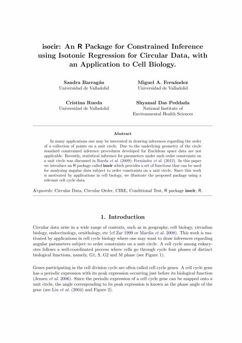
Circular data arise in a wide range of contexts, such as in geography, cell biology, circadianbiology, endocrinology, ornithology, etc (cf Zar 1999 or Mardia et al. 2008). This work is mo-tivated by applications in cell cycle biology where one may want to draw inferences regardingangular parameters subject to order constraints on a unit circle. A cell cycle among eukary-otes follows a well-coordinated process where cells go through cycle four phases of distinctbiological functions, namely, G1, S, G2 and M phase (see Figure 1).

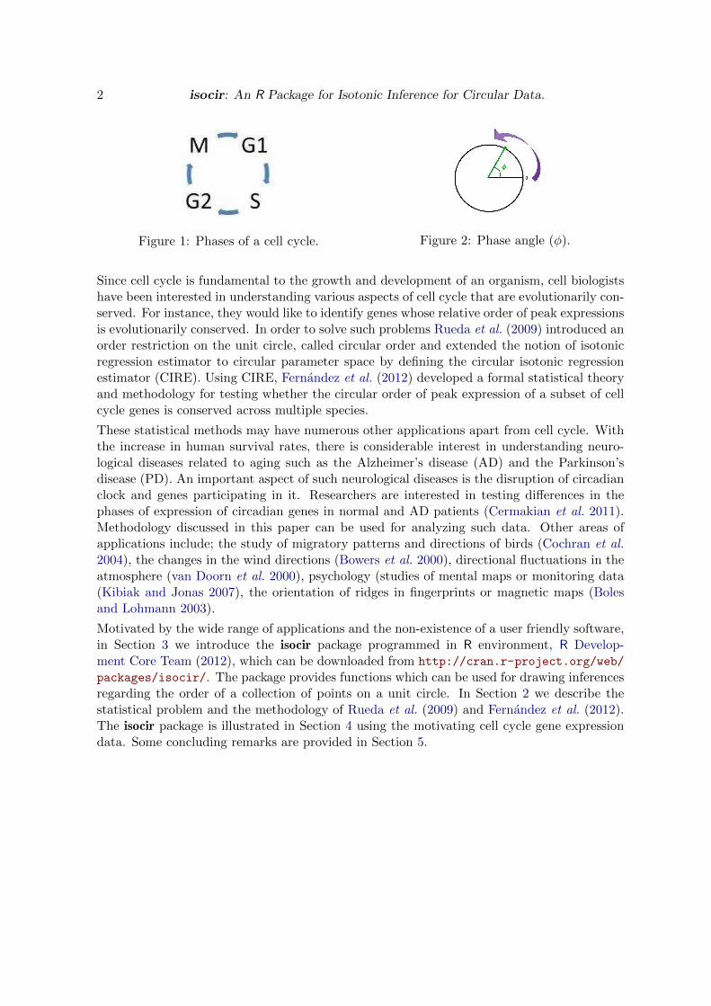
Genes participating in the cell division cycle are often called cell cycle genes. A cell cycle genehas a periodic expression with its peak expression occurring just before its biological function(Jensen et al. 2006). Since the periodic expression of a cell cycle gene can be mapped onto aunit circle, the angle corresponding to its peak expression is known as the phase angle of thegene (see Liu et al. (2004) and Figure 2).

2 isocir: An R Package for Isotonic Inference for Circular Data.

Figure 1: Phases of a cell cycle. Figure 2: Phase angle (φ).

Since cell cycle is fundamental to the growth and development of an organism, cell biologistshave been interested in understanding various aspects of cell cycle that are evolutionarily con-served. For instance, they would like to identify genes whose relative order of peak expressionsis evolutionarily conserved. In order to solve such problems Rueda et al. (2009) introduced anorder restriction on the unit circle, called circular order and extended the notion of isotonicregression estimator to circular parameter space by defining the circular isotonic regressionestimator (CIRE). Using CIRE, Fernandez et al. (2012) developed a formal statistical theoryand methodology for testing whether the circular order of peak expression of a subset of cellcycle genes is conserved across multiple species.

These statistical methods may have numerous other applications apart from cell cycle. Withthe increase in human survival rates, there is considerable interest in understanding neuro-logical diseases related to aging such as the Alzheimer’s disease (AD) and the Parkinson’sdisease (PD). An important aspect of such neurological diseases is the disruption of circadianclock and genes participating in it. Researchers are interested in testing differences in thephases of expression of circadian genes in normal and AD patients (Cermakian et al. 2011).Methodology discussed in this paper can be used for analyzing such data. Other areas ofapplications include; the study of migratory patterns and directions of birds (Cochran et al.2004), the changes in the wind directions (Bowers et al. 2000), directional fluctuations in theatmosphere (van Doorn et al. 2000), psychology (studies of mental maps or monitoring data(Kibiak and Jonas 2007), the orientation of ridges in fingerprints or magnetic maps (Bolesand Lohmann 2003).

Motivated by the wide range of applications and the non-existence of a user friendly software,in Section 3 we introduce the isocir package programmed in R environment, R Develop-ment Core Team (2012), which can be downloaded from http://cran.r-project.org/web/

packages/isocir/. The package provides functions which can be used for drawing inferencesregarding the order of a collection of points on a unit circle. In Section 2 we describe thestatistical problem and the methodology of Rueda et al. (2009) and Fernandez et al. (2012).The isocir package is illustrated in Section 4 using the motivating cell cycle gene expressiondata. Some concluding remarks are provided in Section 5.

Sandra Barragan, Miguel A. Fernandez, Cristina Rueda, Shyamal Das Peddada 3

2. Angular parameters under order constraints

2.1. Circular order restriction

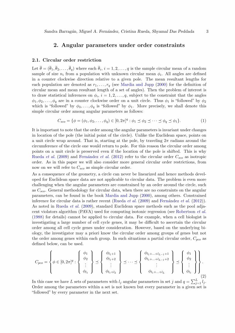
Let θ = (θ1, θ2, . . . , θq) where each θi, i = 1, 2, . . . , q is the sample circular mean of a randomsample of size ni from a population with unknown circular mean φi. All angles are definedin a counter clockwise direction relative to a given pole. The mean resultant lengths foreach population are denoted as r1, . . . , rq (see Mardia and Jupp (2000) for the definition ofcircular mean and mean resultant length of a set of angles). Then the problem of interest isto draw statistical inferences on φi, i = 1, 2, . . . , q, subject to the constraint that the anglesφ1, φ2, . . . , φq are in a counter clockwise order on a unit circle. Thus φ1 is “followed” by φ2which is “followed” by φ3, . . . , φq is “followed” by φ1. More precisely, we shall denote thissimple circular order among angular parameters as follows:

Csco = {φ = (φ1, φ2, . . . , φq) ∈ [0, 2π]q : φ1 � φ2 � · · · � φq � φ1}. (1)

It is important to note that the order among the angular parameters is invariant under changesin location of the pole (the initial point of the circle). Unlike the Euclidean space, points ona unit circle wrap around. That is, starting at the pole, by traveling 2π radians around thecircumference of the circle one would return to pole. For this reason the circular order amongpoints on a unit circle is preserved even if the location of the pole is shifted. This is whyRueda et al. (2009) and Fernandez et al. (2012) refer to the circular order Csco as isotropicorder. As in this paper we will also consider more general circular order restrictions, fromnow on we will refer to Csco as simple circular order.

As a consequence of the geometry, a circle can never be linearized and hence methods devel-oped for Euclidean space data are not applicable to circular data. The problem is even morechallenging when the angular parameters are constrained by an order around the circle, suchas Csco. General methodology for circular data, when there are no constraints on the angularparameters, can be found in the book Mardia and Jupp (2000), among others. Constrainedinference for circular data is rather recent (Rueda et al. (2009) and Fernandez et al. (2012)).As noted in Rueda et al. (2009), standard Euclidean space methods such as the pool adja-cent violators algorithm (PAVA) used for computing isotonic regression (see Robertson et al.(1988) for details) cannot be applied to circular data. For example, when a cell biologist isinvestigating a large number of cell cycle genes, it may be difficult to ascertain the circularorder among all cell cycle genes under consideration. However, based on the underlying bi-ology, the investigator may a priori know the circular order among groups of genes but notthe order among genes within each group. In such situations a partial circular order, Cpco asdefined below, can be used.

Cpco =

φ ∈ [0, 2π]q :

φ1φ2...φl1

�

φl1+1

φl1+2...

φl1+l2

� · · · �

φl1+...+lL−1+1

φl1+...+lL−1+2...

φl1+...+lL

�

φ1φ2...φl1

.

(2)In this case we have L sets of parameters with lj angular parameters in set j and q =

∑Lj=1 lj .

Order among the parameters within a set is not known but every parameter in a given set is“followed” by every parameter in the next set.

4 isocir: An R Package for Isotonic Inference for Circular Data.

2.2. Estimation and testing under circular order restrictions

Analogous to PAVA for Euclidean data, Rueda et al. (2009) derived a circular isotonic regres-sion estimator (CIRE) for estimating angular parameters (φ1, φ2, . . . , φq) subject to a circularorder. The CIRE of φ = (φ1, φ2, . . . , φq), under the constraint (φ1, φ2, . . . , φq)

′ ∈ Csco, is givenby:

φ = arg minφ∈Csco

SCE(φ, θ), (3)

where SCE(φ, θ), defined below, is the sum of circular errors (SCE), a circle analog to theSum of Squared Errors (SSE) used for Euclidean data;

SCE(φ, θ) =

q∑i=1

ri(1− cos(φi − θi)), (4)

where ri are the mean resultant lengths. The CIRE is implemented in the function CIRE ofthe package isocir.

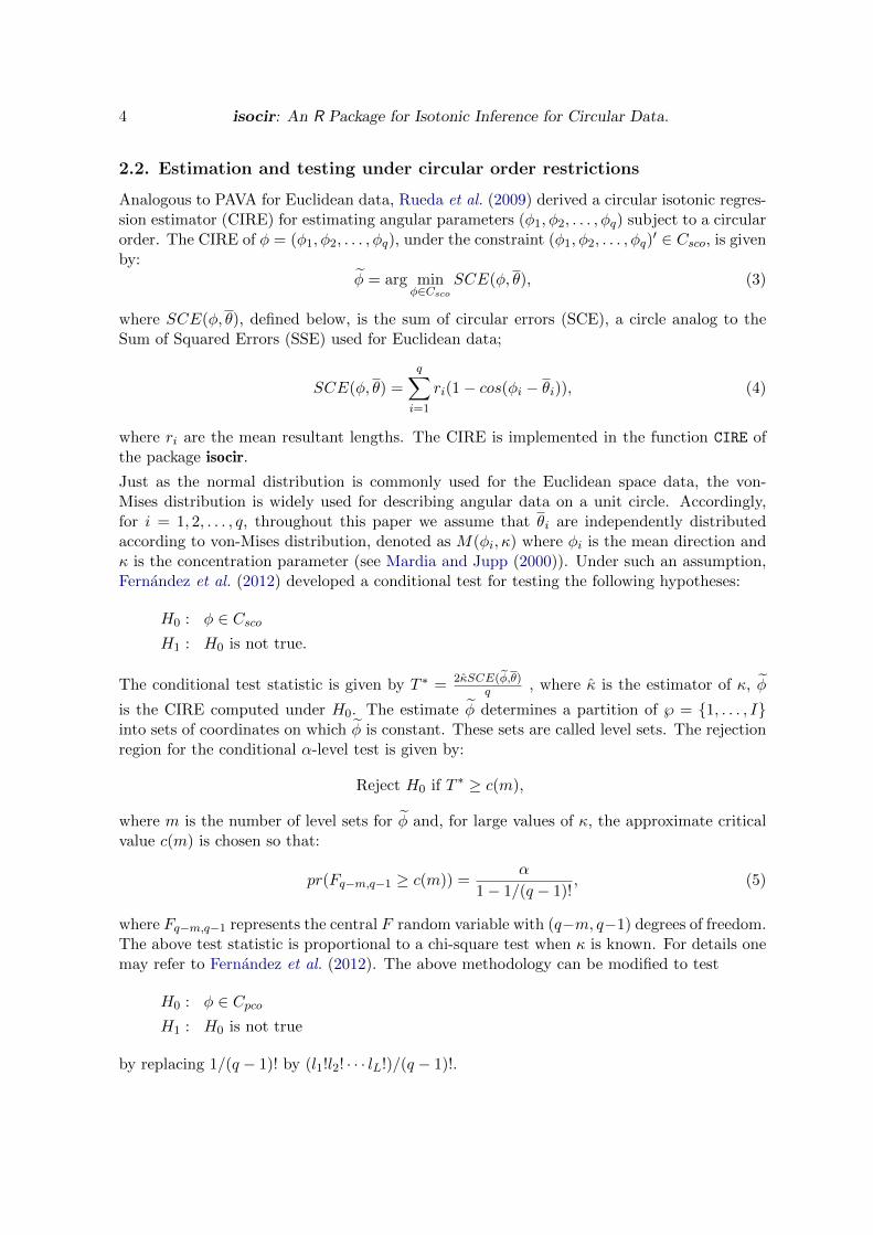
Just as the normal distribution is commonly used for the Euclidean space data, the von-Mises distribution is widely used for describing angular data on a unit circle. Accordingly,for i = 1, 2, . . . , q, throughout this paper we assume that θi are independently distributedaccording to von-Mises distribution, denoted as M(φi, κ) where φi is the mean direction andκ is the concentration parameter (see Mardia and Jupp (2000)). Under such an assumption,Fernandez et al. (2012) developed a conditional test for testing the following hypotheses:

H0 : φ ∈ CscoH1 : H0 is not true.

The conditional test statistic is given by T ∗ = 2κSCE(φ,θ)q , where κ is the estimator of κ, φ

is the CIRE computed under H0. The estimate φ determines a partition of ℘ = {1, . . . , I}into sets of coordinates on which φ is constant. These sets are called level sets. The rejectionregion for the conditional α-level test is given by:

Reject H0 if T ∗ ≥ c(m),

where m is the number of level sets for φ and, for large values of κ, the approximate criticalvalue c(m) is chosen so that:

pr(Fq−m,q−1 ≥ c(m)) =α

1− 1/(q − 1)!, (5)

where Fq−m,q−1 represents the central F random variable with (q−m, q−1) degrees of freedom.The above test statistic is proportional to a chi-square test when κ is known. For details onemay refer to Fernandez et al. (2012). The above methodology can be modified to test

H0 : φ ∈ CpcoH1 : H0 is not true

by replacing 1/(q − 1)! by (l1!l2! · · · lL!)/(q − 1)!.

Sandra Barragan, Miguel A. Fernandez, Cristina Rueda, Shyamal Das Peddada 5

The simulation study performed in Fernandez et al. (2012) suggests that the power of this testis quite reasonable. Notice that, for a given data set, the p-value obtained by using the abovemethodology may serve as a useful goodness of fit criterion when comparing two or moreplausible circular orders among a set of angular parameters. Larger values may suggest thatthe estimations are closer to the presumed circular order. Thus the statistical methodologydeveloped in Fernandez et al. (2012) can be used not only for testing relative order amongthe parameters. It can be also useful for selecting a “best fitting” circular order among severalcircular order candidates.

These tests are implemented in the function cond.test in the R package isocir introduced inthe next Section.

3. Package isocir

We start this section by giving some background on R packages for isotonic regression andanalysis of circular data. We then describe the structure of our package isocir and illustrateit by some examples.

3.1. Related packages

As isotonic regression is a well-known and widely used technique there are many packages inR for performing isotonic regression, such as:

� isotone (de Leeuw et al. 2011): Active set and generalized PAVA for isotone optimiza-tion.

� Iso (Turner 2009): Functions to perform isotonic regression.

� ordMonReg (Balabdaoui et al. 2009): Compute least squares estimates of one boundedor two ordered isotonic regression curves.

Similarly, there are several packages in R for analyzing circular data, such as:

� CircStats (Lund and Agostinelli 2009): The implementations of the Circular Statisticsfrom “Topics in circular Statistics” Jammalamadaka and SenGupta (2001). It is an Rport from the S-plus library with the same name.

� circular (Agostinelli and Lund 2011): This package expands in several ways the Circ-Stats package.

Since none of the existing packages for circular data are applicable for analyzing circular dataunder constraints, in this article we introduce the software package “isotonic inference forcircular data”, with the acronym isocir, for analyzing circular data under constraints. Ourpackage depends on circular (see (Agostinelli and Lund 2011)) and combinat (see (Chasalow2010)). These packages should be installed in the computer before loading isocir.

3.2. Package structure

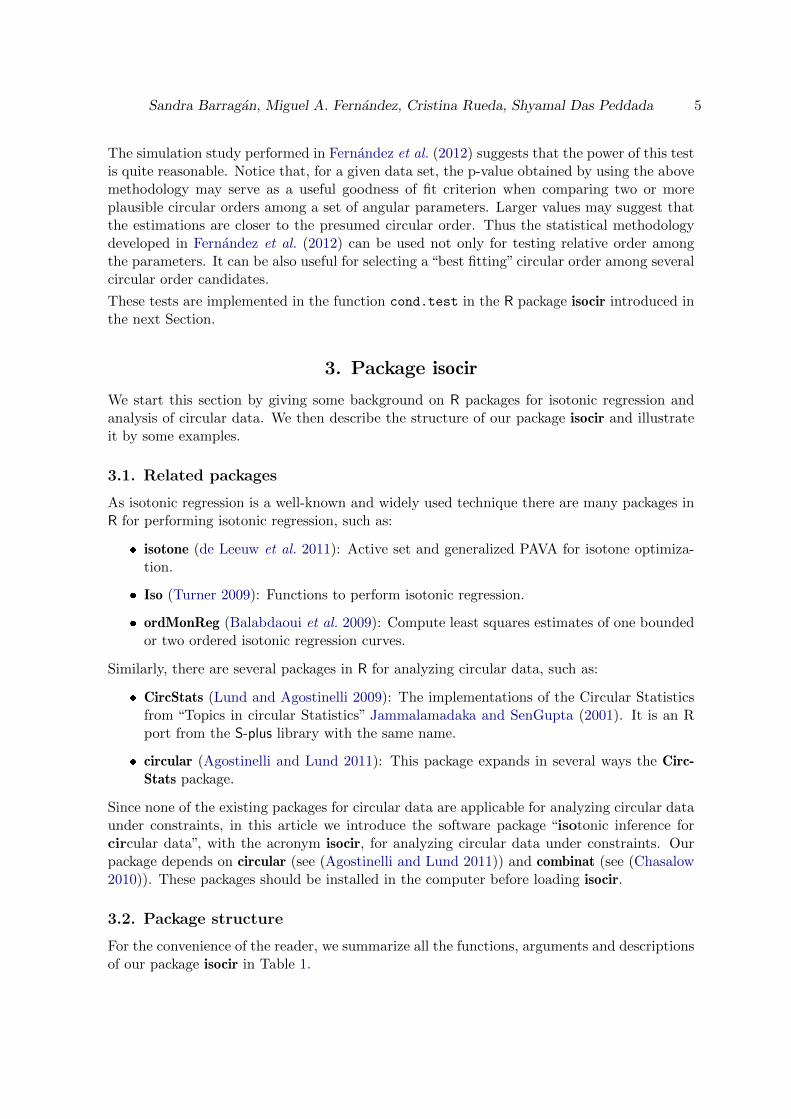
For the convenience of the reader, we summarize all the functions, arguments and descriptionsof our package isocir in Table 1.

6 isocir: An R Package for Isotonic Inference for Circular Data.

Functions Arguments Description

sce (arg1, arg2, meanrl) SCE

mrl (data) Mean resultant length

CIRE (data, groups, circular) Calculates the CIRE

cond.test (data, groups, kappa) Conditional test

isocir (cirmeans,SCE,CIRE,pvalue,kappa) S3 object of class isocir

is.isocir (x) Checks class isocir

print.isocir (x,decCIRE,decpvalue,deckappa,...) Prints an object of class isocir

plot.isocir (x, option,...) Plots an object of class isocir

Table 1: Summary of the components of the package isocir.

In the following we describe each function of the software in detail.

� Functions sce() and mrl()

The auxiliary function sce computes the sum of circular errors between a given q-dimensionalvector (denoted by arg1) and one or more q-dimensional vectors (denoted by arg2). Thefunction mrl computes the mean resultant length for the input data.

� Function CIRE()

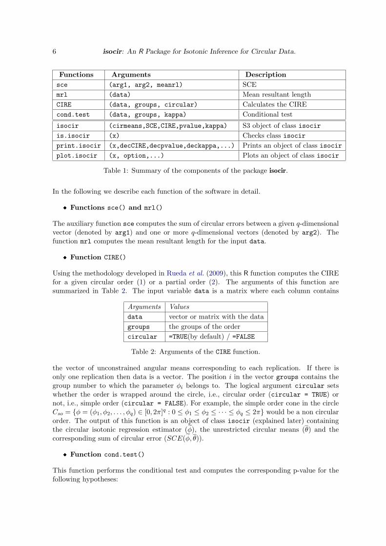
Using the methodology developed in Rueda et al. (2009), this R function computes the CIREfor a given circular order (1) or a partial order (2). The arguments of this function aresummarized in Table 2. The input variable data is a matrix where each column contains

Arguments Values

data vector or matrix with the data

groups the groups of the order

circular =TRUE(by default) / =FALSE

Table 2: Arguments of the CIRE function.

the vector of unconstrained angular means corresponding to each replication. If there isonly one replication then data is a vector. The position i in the vector groups contains thegroup number to which the parameter φi belongs to. The logical argument circular setswhether the order is wrapped around the circle, i.e., circular order (circular = TRUE) ornot, i.e., simple order (circular = FALSE). For example, the simple order cone in the circleCso = {φ = (φ1, φ2, . . . , φq) ∈ [0, 2π]q : 0 ≤ φ1 ≤ φ2 ≤ · · · ≤ φq ≤ 2π} would be a non circularorder. The output of this function is an object of class isocir (explained later) containingthe circular isotonic regression estimator (φ), the unrestricted circular means (θ) and thecorresponding sum of circular error (SCE(φ, θ)).

� Function cond.test()

This function performs the conditional test and computes the corresponding p-value for thefollowing hypotheses:

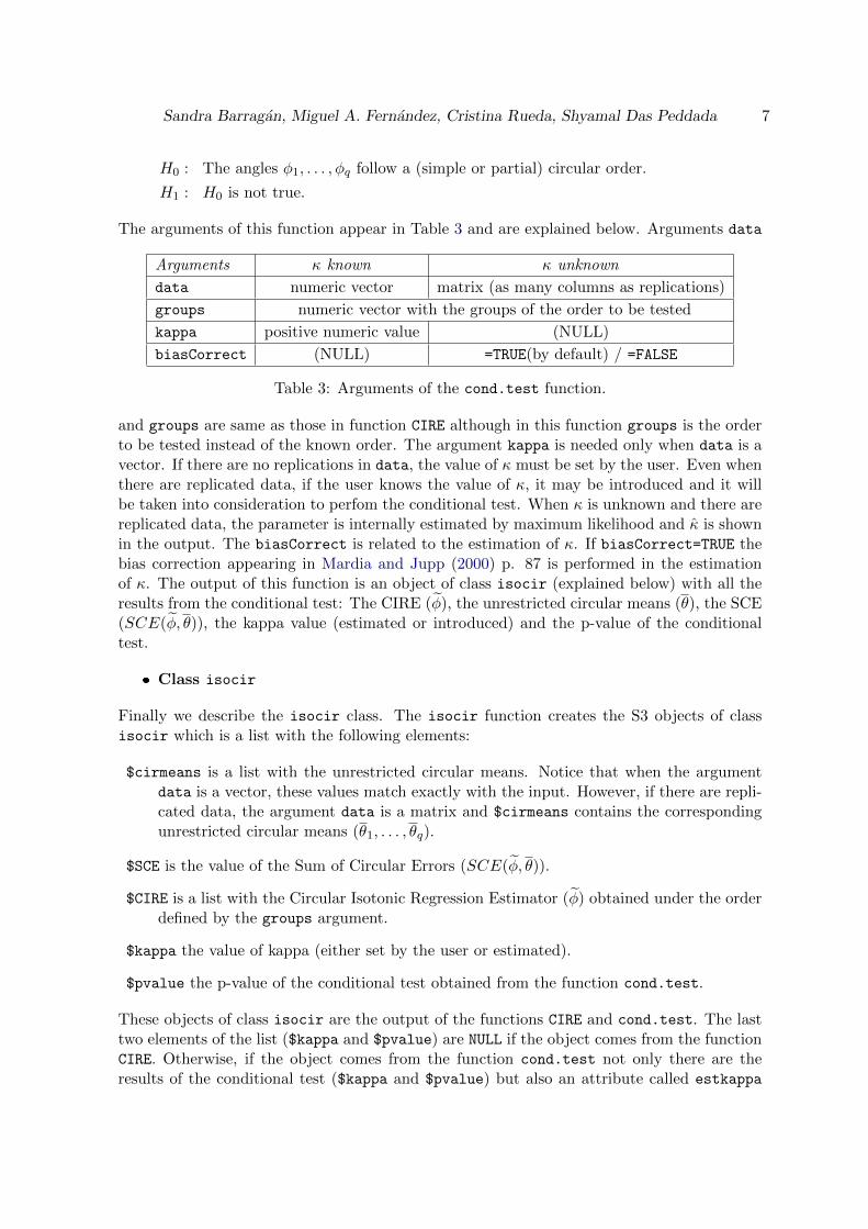
Sandra Barragan, Miguel A. Fernandez, Cristina Rueda, Shyamal Das Peddada 7

H0 : The angles φ1, . . . , φq follow a (simple or partial) circular order.

H1 : H0 is not true.

The arguments of this function appear in Table 3 and are explained below. Arguments data

Arguments κ known κ unknown

data numeric vector matrix (as many columns as replications)

groups numeric vector with the groups of the order to be tested

kappa positive numeric value (NULL)

biasCorrect (NULL) =TRUE(by default) / =FALSE

Table 3: Arguments of the cond.test function.

and groups are same as those in function CIRE although in this function groups is the orderto be tested instead of the known order. The argument kappa is needed only when data is avector. If there are no replications in data, the value of κ must be set by the user. Even whenthere are replicated data, if the user knows the value of κ, it may be introduced and it willbe taken into consideration to perfom the conditional test. When κ is unknown and there arereplicated data, the parameter is internally estimated by maximum likelihood and κ is shownin the output. The biasCorrect is related to the estimation of κ. If biasCorrect=TRUE thebias correction appearing in Mardia and Jupp (2000) p. 87 is performed in the estimationof κ. The output of this function is an object of class isocir (explained below) with all theresults from the conditional test: The CIRE (φ), the unrestricted circular means (θ), the SCE(SCE(φ, θ)), the kappa value (estimated or introduced) and the p-value of the conditionaltest.

� Class isocir

Finally we describe the isocir class. The isocir function creates the S3 objects of classisocir which is a list with the following elements:

$cirmeans is a list with the unrestricted circular means. Notice that when the argumentdata is a vector, these values match exactly with the input. However, if there are repli-cated data, the argument data is a matrix and $cirmeans contains the correspondingunrestricted circular means (θ1, . . . , θq).

$SCE is the value of the Sum of Circular Errors (SCE(φ, θ)).

$CIRE is a list with the Circular Isotonic Regression Estimator (φ) obtained under the orderdefined by the groups argument.

$kappa the value of kappa (either set by the user or estimated).

$pvalue the p-value of the conditional test obtained from the function cond.test.

These objects of class isocir are the output of the functions CIRE and cond.test. The lasttwo elements of the list ($kappa and $pvalue) are NULL if the object comes from the functionCIRE. Otherwise, if the object comes from the function cond.test not only there are theresults of the conditional test ($kappa and $pvalue) but also an attribute called estkappa

8 isocir: An R Package for Isotonic Inference for Circular Data.

will inform (or rather remind) the user if the value in $kappa has been internally estimatedor introduced as a known input.

Some S3 methods have also been defined for the class isocir:

� isocir(cirmeans = NULL, SCE = NULL, CIRE = NULL, pvalue = NULL,

kappa = NULL): This function creates an object of class isocir.

� is.isocir(x): This function checks whether the object x is of class isocir.

� print.isocir(x, decCIRE, decpvalue, deckappa, ...): This S3 method is usedto print an object x of class isocir. The number of decimal places can be chosen.

� plot.isocir(x, option = c("CIRE", "cirmeans"), ...): This S3 method is usedto plot an object x of class isocir. The argument option gives the user the optionto plot the points of the Circular Isotonic Regression Estimator (by default) or theunrestricted circular means.

3.3. Examples

In this section we provide examples to illustrate isocir.

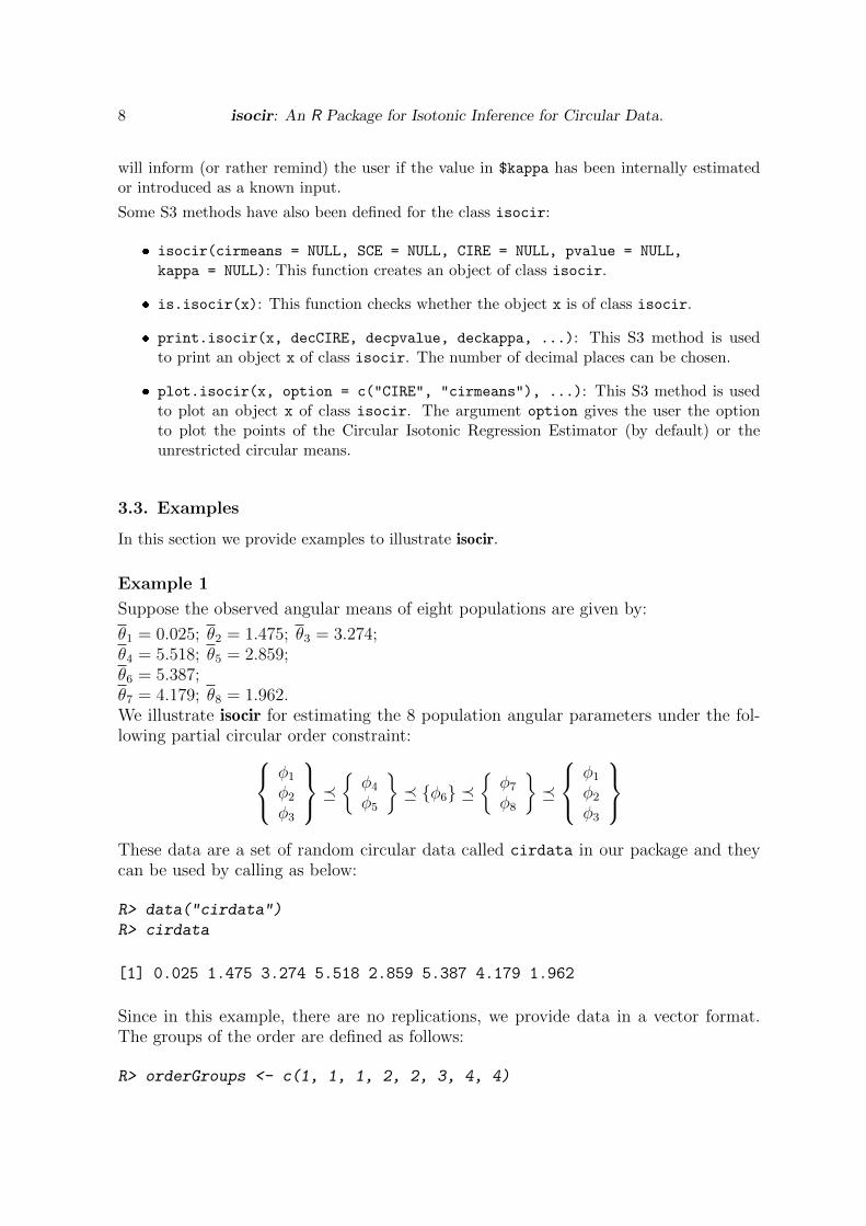
Example 1

Suppose the observed angular means of eight populations are given by:

θ1 = 0.025; θ2 = 1.475; θ3 = 3.274;θ4 = 5.518; θ5 = 2.859;θ6 = 5.387;θ7 = 4.179; θ8 = 1.962.We illustrate isocir for estimating the 8 population angular parameters under the fol-lowing partial circular order constraint: φ1

φ2

φ3

�{φ4

φ5

}� {φ6} �

{φ7

φ8

}�

φ1

φ2

φ3

These data are a set of random circular data called cirdata in our package and theycan be used by calling as below:

R> data("cirdata")

R> cirdata

[1] 0.025 1.475 3.274 5.518 2.859 5.387 4.179 1.962

Since in this example, there are no replications, we provide data in a vector format.The groups of the order are defined as follows:

R> orderGroups <- c(1, 1, 1, 2, 2, 3, 4, 4)

Sandra Barragan, Miguel A. Fernandez, Cristina Rueda, Shyamal Das Peddada 9

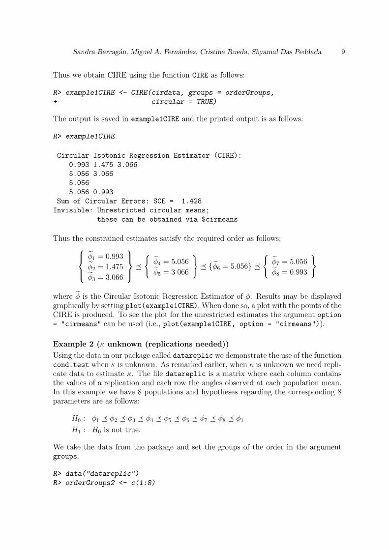
Thus we obtain CIRE using the function CIRE as follows:

R> example1CIRE <- CIRE(cirdata, groups = orderGroups,

+ circular = TRUE)

The output is saved in example1CIRE and the printed output is as follows:

R> example1CIRE

Circular Isotonic Regression Estimator (CIRE):

0.993 1.475 3.066

5.056 3.066

5.056

5.056 0.993

Sum of Circular Errors: SCE = 1.428

Invisible: Unrestricted circular means;

these can be obtained via $cirmeans

Thus the constrained estimates satisfy the required order as follows:φ1 = 0.993

φ2 = 1.475

φ3 = 3.066

�{φ4 = 5.056

φ5 = 3.066

}� {φ6 = 5.056} �

{φ7 = 5.056

φ8 = 0.993

}

where φ is the Circular Isotonic Regression Estimator of φ. Results may be displayedgraphically by setting plot(example1CIRE). When done so, a plot with the points of theCIRE is produced. To see the plot for the unrestricted estimates the argument option= "cirmeans" can be used (i.e., plot(example1CIRE, option = "cirmeans")).

Example 2 (κ unknown (replications needed))

Using the data in our package called datareplic we demonstrate the use of the functioncond.test when κ is unknown. As remarked earlier, when κ is unknown we need repli-cate data to estimate κ. The file datareplic is a matrix where each column containsthe values of a replication and each row the angles observed at each population mean.In this example we have 8 populations and hypotheses regarding the corresponding 8parameters are as follows:

H0 : φ1 � φ2 � φ3 � φ4 � φ5 � φ6 � φ7 � φ8 � φ1

H1 : H0 is not true.

We take the data from the package and set the groups of the order in the argumentgroups.

R> data("datareplic")

R> orderGroups2 <- c(1:8)

10 isocir: An R Package for Isotonic Inference for Circular Data.

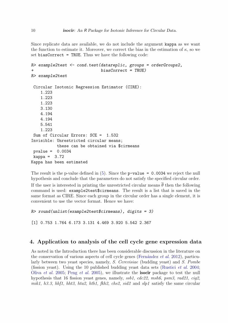
Since replicate data are available, we do not include the argument kappa as we wantthe function to estimate it. Moreover, we correct the bias in the estimation of κ, so weset biasCorrect = TRUE. Thus we have the following code:

R> example2test <- cond.test(datareplic, groups = orderGroups2,

+ biasCorrect = TRUE)

R> example2test

Circular Isotonic Regression Estimator (CIRE):

1.223

1.223

1.223

3.130

4.194

4.194

5.541

1.223

Sum of Circular Errors: SCE = 1.532

Invisible: Unrestricted circular means;

these can be obtained via $cirmeans

pvalue = 0.0034

kappa = 3.72

Kappa has been estimated

The result is the p-value defined in (5). Since the p-value = 0.0034 we reject the nullhypothesis and conclude that the parameters do not satisfy the specified circular order.

If the user is interested in printing the unrestricted circular means θ then the followingcommand is used: example2test$cirmeans. The result is a list that is saved in thesame format as CIRE. Since each group in the circular order has a single element, it isconvenient to use the vector format. Hence we have:

R> round(unlist(example2test$cirmeans), digits = 3)

[1] 0.753 1.764 6.173 3.131 4.469 3.920 5.542 2.367

4. Application to analysis of the cell cycle gene expression data

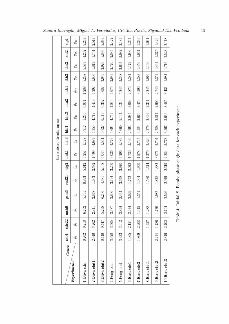
As noted in the Introduction there has been considerable discussion in the literature onthe conservation of various aspects of cell cycle genes (Fernandez et al. 2012), particu-larly between two yeast species, namely, S. Cerevisiae (budding yeast) and S. Pombe(fission yeast). Using the 10 published budding yeast data sets (Rustici et al. 2004;Oliva et al. 2005; Peng et al. 2005), we illustrate the isocir package to test the nullhypothesis that 16 fission yeast genes, namely, ssb1, cdc22, msh6, psm3, rad21, cig2,mik1, h3.3, hhf1, hht3, hta2, htb1, fkh2, chs2, sid2 and slp1 satisfy the same circular

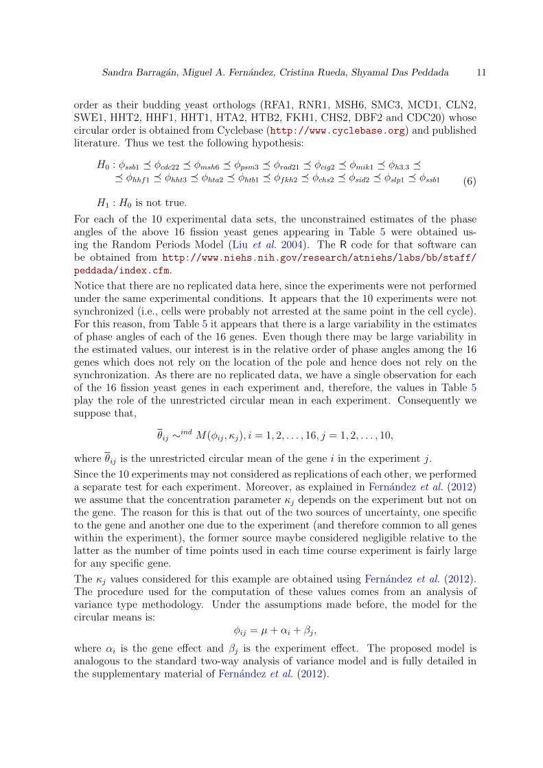
Sandra Barragan, Miguel A. Fernandez, Cristina Rueda, Shyamal Das Peddada 11

order as their budding yeast orthologs (RFA1, RNR1, MSH6, SMC3, MCD1, CLN2,SWE1, HHT2, HHF1, HHT1, HTA2, HTB2, FKH1, CHS2, DBF2 and CDC20) whosecircular order is obtained from Cyclebase (http://www.cyclebase.org) and publishedliterature. Thus we test the following hypothesis:

H0 : φssb1 � φcdc22 � φmsh6 � φpsm3 � φrad21 � φcig2 � φmik1 � φh3.3 �� φhhf1 � φhht3 � φhta2 � φhtb1 � φfkh2 � φchs2 � φsid2 � φslp1 � φssb1

H1 : H0 is not true.

(6)

For each of the 10 experimental data sets, the unconstrained estimates of the phaseangles of the above 16 fission yeast genes appearing in Table 5 were obtained us-ing the Random Periods Model (Liu et al. 2004). The R code for that software canbe obtained from http://www.niehs.nih.gov/research/atniehs/labs/bb/staff/

peddada/index.cfm.

Notice that there are no replicated data here, since the experiments were not performedunder the same experimental conditions. It appears that the 10 experiments were notsynchronized (i.e., cells were probably not arrested at the same point in the cell cycle).For this reason, from Table 5 it appears that there is a large variability in the estimatesof phase angles of each of the 16 genes. Even though there may be large variability inthe estimated values, our interest is in the relative order of phase angles among the 16genes which does not rely on the location of the pole and hence does not rely on thesynchronization. As there are no replicated data, we have a single observation for eachof the 16 fission yeast genes in each experiment and, therefore, the values in Table 5play the role of the unrestricted circular mean in each experiment. Consequently wesuppose that,

θij ∼ind M(φij, κj), i = 1, 2, . . . , 16, j = 1, 2, . . . , 10,

where θij is the unrestricted circular mean of the gene i in the experiment j.

Since the 10 experiments may not considered as replications of each other, we performeda separate test for each experiment. Moreover, as explained in Fernandez et al. (2012)we assume that the concentration parameter κj depends on the experiment but not onthe gene. The reason for this is that out of the two sources of uncertainty, one specificto the gene and another one due to the experiment (and therefore common to all geneswithin the experiment), the former source maybe considered negligible relative to thelatter as the number of time points used in each time course experiment is fairly largefor any specific gene.

The κj values considered for this example are obtained using Fernandez et al. (2012).The procedure used for the computation of these values comes from an analysis ofvariance type methodology. Under the assumptions made before, the model for thecircular means is:

φij = µ+ αi + βj,

where αi is the gene effect and βj is the experiment effect. The proposed model isanalogous to the standard two-way analysis of variance model and is fully detailed inthe supplementary material of Fernandez et al. (2012).

12 isocir: An R Package for Isotonic Inference for Circular Data.

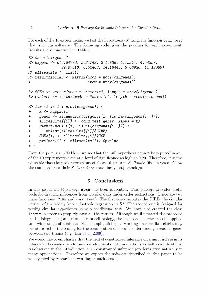
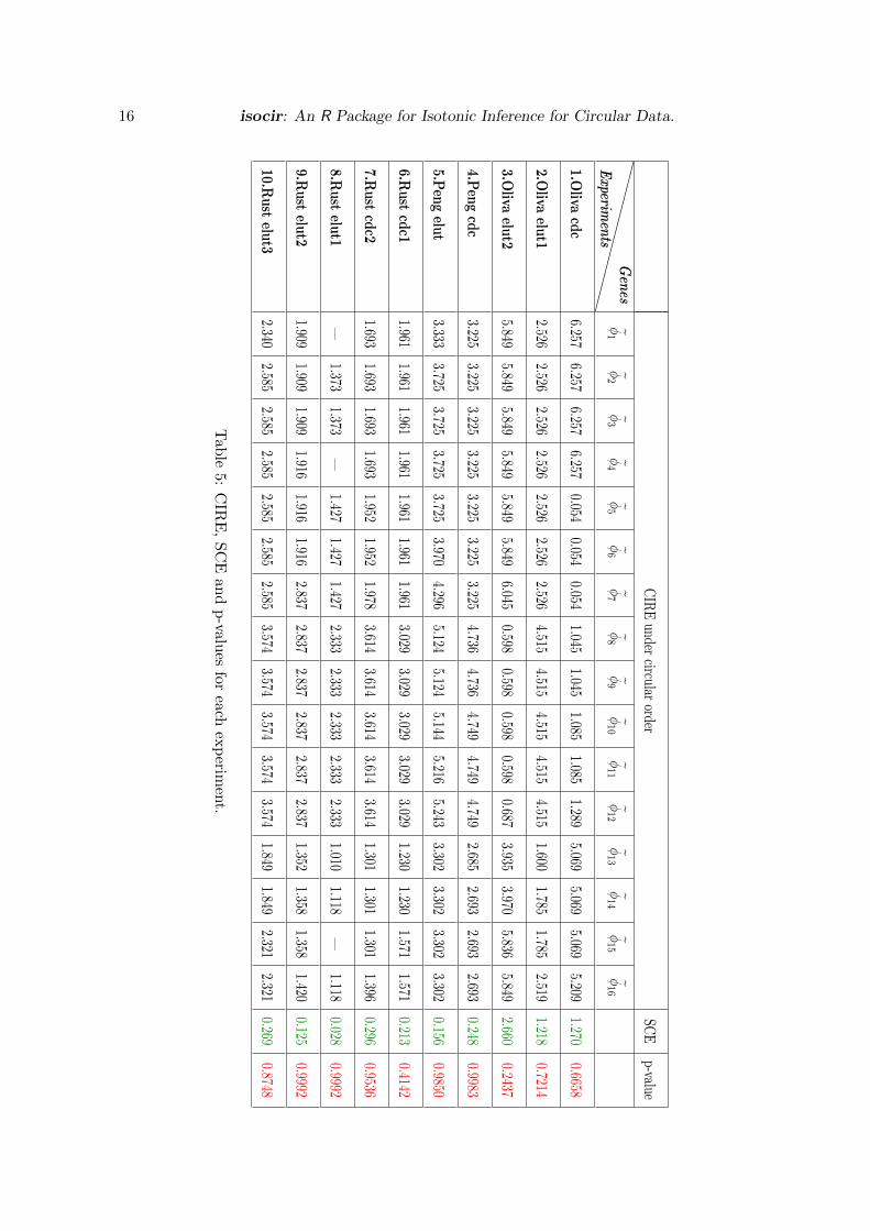
For each of the 10 experiments, we test the hypothesis (6) using the function cond.test

that is in our software. The following code gives the p-values for each experiment.Results are summarized in Table 5.

R> data("cirgenes")

R> kappas <- c(2.64773, 3.24742, 2.15936, 4.15314, 4.54357,

+ 29.07610, 6.51408, 14.19445, 5.66920, 11.12889)

R> allresults <- list()

R> resultIsoCIRE <- matrix(ncol = ncol(cirgenes),

+ nrow = nrow(cirgenes))

R> SCEs <- vector(mode = "numeric", length = nrow(cirgenes))

R> pvalues <- vector(mode = "numeric", length = nrow(cirgenes))

R> for (i in 1 : nrow(cirgenes)) {

+ k <- kappas[i]

+ genes <- as.numeric(cirgenes[i, !is.na(cirgenes[i, ])])

+ allresults[[i]] <- cond.test(genes, kappa = k)

+ resultIsoCIRE[i, !is.na(cirgenes[i, ])] <-

+ unlist(allresults[[i]]$CIRE)

+ SCEs[i] <- allresults[[i]]$SCE

+ pvalues[i] <- allresults[[i]]$pvalue

+ }

From the p-values in Table 5, we see that the null hypothesis cannot be rejected in anyof the 10 experiments even at a level of significance as high as 0.20. Therefore, it seemsplausible that the peak expressions of these 16 genes in S. Pombe (fission yeast) followthe same order as their S. Cerevisiae (budding yeast) orthologs.

5. Conclusions

In this paper the R package isocir has been presented. This package provides usefultools for drawing inferences from circular data under order restrictions. There are twomain functions (CIRE and cond.test). The first one computes the CIRE, the circularversion of the widely known isotonic regression in Rq. The second one is designed fortesting circular hypotheses using a conditional test. We have also created the classisocir in order to properly save all the results. Although we illustrated the proposedmethodology using an example from cell biology, the proposed software can be appliedto a wide range of contexts. For example, biologists working on circadian clocks maybe interested in the testing for the conservation of circular order among circadian genesbetween two tissues (e.g., Liu et al. 2006).

We would like to emphasize that the field of constrained inference on a unit circle is in itsinfancy and is wide open for new developments both in methods as well as applications.As observed in the introduction, such constrained inference problems arise naturally inmany applications. Therefore we expect the software described in this paper to bewidely used by researchers working in such areas.

Sandra Barragan, Miguel A. Fernandez, Cristina Rueda, Shyamal Das Peddada 13

Acknowledgments

SB’s, MAF’s and CR’s research was partially supported by Spanish MCI grant MTM2009-11161. SB’s work has been partially financed by Junta de Castilla y Leon, Consejerıade Educacion and the European Social Fund within the P.O. Castilla y Leon 2007-2013programme. SDP’s research [in part] was supported by the Intramural Research Pro-gram of the NIH, National Institute of Environmental Health Sciences (Z01 ES101744-04). We thank Dr. Leping Li, Keith Shockley, the anonymous reviewers, the associateeditor and the editor for several useful comments which improved the presentation ofthis manuscript.

References

Agostinelli C, Lund U (2011). circular: Circular Statistics. CA: Department ofEnvironmental Sciences, Informatics and Statistics, Ca’ Foscari University, Venice,Italy. UL: Department of Statistics, California Polytechnic State University, SanLuis Obispo, California, USA. R package version 0.4-3, URL https://r-forge.

r-project.org/projects/circular/.

Balabdaoui F, Rufibach K, Santambrogio F (2009). OrdMonReg: Compute LeastSquares Estimates of One Bounded or Two Ordered Isotonic Regression Curves.R package version 1.0.2, URL http://CRAN.R-project.org/package=OrdMonReg.

Boles L, Lohmann K (2003). “True Navigation and Magnetic Maps in Spiny Lobsters.”Nature, 421, 60–63.

Bowers J, Morton I, Mould G (2000). “Directional Statistics of the Wind and Waves.”Applied Ocean Research, 22, 13–30.

Cermakian N, Lamont E, Bourdeau P, Boivin D (2011). “Circadian Clock Gene Expres-sion in Brain Regions of Alzheimer’s Disease Patients and Control Subjects.” Journalof Biological Rhythms, 26, 160–170.

Chasalow S (2010). combinat: Combinatorics Utilities. R package version 0.0-8, URLhttp://CRAN.R-project.org/package=combinat.

Cochran W, Mouritsen H, Wikelski M (2004). “Migrating Songbirds Recalibrate TheirMagnetic Compass Daily from Twilight Cues.” Science, 304, 405–408.

de Leeuw J, Hornik K, Mair P (2011). isotone: Active Set and Generalized PAVA forIsotone Optimization. R package version 1.0-1, URL http://CRAN.R-project.org/

package=isotone.

Fernandez M, Rueda C, Peddada S (2012). “Identification of a Core Set of Signa-ture Cell Cycle Genes Whose Relative Order of Time to Peak Expression is Con-served Across Species.” Nucleic Acids Research, 40(7), 2823–2832. URL http:

//nar.oxfordjournals.org/content/40/7/2823.

14 isocir: An R Package for Isotonic Inference for Circular Data.

Jammalamadaka S, SenGupta A (2001). Topics in Circular Statistics. World Scientific.

Jensen JL Jensen T, Lichtenberg U, Brunak S, Bork P (2006). “Co-Evolution of Tran-scriptional and Post-Translational Cell-Cycle Regulation.” Nature, 443, 594–597.

Kibiak T, Jonas C (2007). “Applying Circular Statistics to the Analysis of MonitoringData.” European Journal of Psychological Assessment, 23, 227–237.

Liu D, Peddada S, Li L, Weinberg C (2006). “Phase Analysis of Circadian-RelatedGenes in Two Tissues.” BMC Bioinformatics, 7, 87.

Liu D, Umbach D, Peddada S, Li L, Crockett P, Weinberg C (2004). “A RandomPeriods Model for Expression of Cell-Cycle Genes.” PNAS, 101(19), 7240–7245.

Lund U, Agostinelli C (2009). CircStats: Circular Statistics, from ”Topics in Circu-lar Statistics” (2001). R package version 0.2-4, URL http://CRAN.R-project.org/

package=CircStats.

Mardia K, Hughes G, Taylor C, Singh H (2008). “A Multivariate von Mises Distributionwith Applications to Bioinformatics.” Canadian Journal of Statistics, 36, 99–109.

Mardia K, Jupp P (2000). Directional Statistics. John Wiley & Sons.

Oliva A, Rosebrock A, Ferrezuelo F, Pyne S, Chen H, Skiena S, Futcher B, LeatherwoodJ (2005). “The Cell-Cycle-Regulated Genes of Schizosaccharomyces Pombe.” Plos.Biology, 3, 1239–1260.

Peng X, Karuturi R, Miller L, Lin K, Jia Y, Kondu P, Wang L, Wong L, Liu E,Balasubramanian M, Liu J (2005). “Identification of Cell Cycle-Regulated Genes inFission Yeast.” The American Society for Cell Biology, 16, 1026–1042.

R Development Core Team (2012). R: A Language and Environment for StatisticalComputing. R Foundation for Statistical Computing, Vienna, Austria. ISBN 3-900051-07-0, URL http://www.R-project.org.

Robertson T, Wright F, Dykstra R (1988). Order Restricted Statitical Inference. JohnWiley & Sons.

Rueda C, Fernandez M, Peddada S (2009). “Estimation of Parameters Subject to OrderRestrictions on a Circle with Application to Estimation of Phase Angles of Cell-CycleGenes.” Journal of the American Statistical Association, 104(485), 338–347.

Rustici G, Mata J, Kivinen K, Lio P, Penkett C, Burns G, Hayles J, Brazma A, NurseP, Bahler J (2004). “Periodic Gene Expression Program of the Fission Yeast CellCycle.” Nature Genetics, 36, 809–817.

Turner R (2009). Iso: Functions to Perform Isotonic Regression. R package version 0.0-8, URL http://CRAN.R-project.org/package=Iso.

van Doorn E, Dhruva B, Sreenivasan K, Cassella V (2000). “Statistics of Wind Directionand Its Increments.” Physics of Fluids, 12, 1529–1534.

Zar J (1999). Biostatistical Analysis. Prentice Hall.

Sandra Barragan, Miguel A. Fernandez, Cristina Rueda, Shyamal Das Peddada 15

Unr

estr

icte

dci

rcul

arm

eans

``

``

```

```

``

Exp

erim

ents

Gen

esssb1

cdc2

2msh

6psm

3ra

d21

cig2

mik1

h3.3

hhf1

hht

3ht

a2ht

b1

fkh2

chs2

sid2

slp1

θ 1θ 2

θ 3θ 4

θ 5θ 6

θ 7θ 8

θ 9θ 1

0θ 1

1θ 1

2θ 1

3θ 1

4θ 1

5θ 1

6

1.Oliva

cdc

0.20

20.

218

6.26

25.

765

0.89

35.

612

6.25

71.

178

0.91

21.

200

0.97

11.

289

5.29

85.

597

4.25

25.

209

2.Oliva

elut1

2.94

03.

262

2.81

12.

848

1.60

32.

382

1.70

94.

689

4.35

54.

717

4.41

94.

397

1.60

01.

819

1.75

12.

519

3.Oliva

elut2

0.44

00.

447

5.25

86.

206

4.38

15.

458

6.04

51.

541

0.72

76.

115

0.35

20.

687

3.93

53.

970

5.83

65.

896

4.Pen

gcd

c3.

328

3.56

53.

387

2.80

63.

194

3.26

03.

026

4.77

94.

694

4.75

54.

816

4.67

52.

685

2.77

02.

885

2.42

2

5.Pen

gelut

3.33

33.

912

3.89

43.

444

3.64

83.

970

4.29

65.

189

5.06

05.

144

5.21

65.

243

3.33

83.

607

3.08

23.

185

6.Rust

cdc1

1.96

52.

151

2.03

42.

029

1.74

22.

073

1.73

03.

130

2.99

33.

085

3.06

32.

873

1.28

11.

179

1.90

61.

237

7.Rust

cdc2

1.80

92.

208

1.41

51.

351

1.96

41.

940

1.97

83.

745

3.58

43.

670

3.47

93.

590

1.38

31.

456

1.06

41.

396

8.Rust

elut1

—1.

457

1.28

8—

1.53

01.

374

1.37

92.

420

2.27

92.

409

2.31

12.

245

1.01

01.

146

—1.

091

9.Rust

elut2

2.21

41.

786

1.73

01.

987

1.87

81.

882

3.07

12.

704

2.78

82.

814

2.90

92.

740

1.35

21.

441

1.27

51.

420

10.R

ust

elut3

2.34

02.

702

2.70

42.

526

2.97

92.

319

2.28

43.

773

3.56

73.

636

3.46

53.

431

1.98

11.

716

2.52

32.

118

Table

4:

Init

ial

S.

Pom

be

ph

ase

angl

edat

afo

rea

chex

per

imen

t.

16 isocir: An R Package for Isotonic Inference for Circular Data.

CIR

Eunder

circularorder

SCE

p-value``

``

```

```

``

Experim

ents

Gen

esφ1

φ2

φ3

φ4

φ5

φ6

φ7

φ8

φ9

φ10

φ11

φ12

φ13

φ14

φ15

φ16

1.Oliva

cdc6.257

6.2576.257

6.2570.054

0.0540.054

1.0451.045

1.0851.085

1.2895.069

5.0695.069

5.2091.270

0.6658

2.Oliva

elut12.526

2.5262.526

2.5262.526

2.5262.526

4.5154.515

4.5154.515

4.5151.600

1.7851.785

2.5191.218

0.7214

3.Oliva

elut25.849

5.8495.849

5.8495.849

5.8496.045

0.5980.598

0.5980.598

0.6873.935

3.9705.836

5.8492.660

0.2437

4.Peng

cdc3.225

3.2253.225

3.2253.225

3.2253.225

4.7364.736

4.7494.749

4.7492.685

2.6932.693

2.6930.248

0.9983

5.Peng

elut3.333

3.7253.725

3.7253.725

3.9704.296

5.1245.124

5.1445.216

5.2433.302

3.3023.302

3.3020.156

0.9850

6.Rust

cdc11.961

1.9611.961

1.9611.961

1.9611.961

3.0293.029

3.0293.029

3.0291.230

1.2301.571

1.5710.213

0.4142

7.Rust

cdc21.693

1.6931.693

1.6931.952

1.9521.978

3.6143.614

3.6143.614

3.6141.301

1.3011.301

1.3960.296

0.9536

8.Rust

elut1—

1.3731.373

—1.427

1.4271.427

2.3332.333

2.3332.333

2.3331.010

1.118—

1.1180.028

0.9992

9.Rust

elut21.909

1.9091.909

1.9161.916

1.9162.837

2.8372.837

2.8372.837

2.8371.352

1.3581.358

1.4200.125

0.9992

10.Rust

elut32.340

2.5852.585

2.5852.585

2.5852.585

3.5743.574

3.5743.574

3.5741.849

1.8492.321

2.3210.269

0.8748

Tab

le5:

CIR

E,

SC

Ean

dp-valu

esfor

eachex

perim

ent.

Sandra Barragan, Miguel A. Fernandez, Cristina Rueda, Shyamal Das Peddada 17

Affiliation:

Sandra Barragan, Miguel A. Fernandez, Cristina RuedaDepartamento de Estadıstica e Investigacion OperativaInstituto de Matematicas (IMUVA)Universidad de ValladolidValladolid, SpainE-mail: sandraba@eio.uva.es,miguelaf@eio.uva.es,crueda@eio.uva.es

URL: http://www.eio.uva.es/~sandra/http://www.eio.uva.es/~miguel/

http://www.eio.uva.es/~cristina/

Shyamal D. PeddadaBiostatistics BranchNational Institute of Environmental Health SciencesResearch Triangle ParkNC 27709, USAE-mail: peddada@niehs.nih.gov,URL: http://www.niehs.nih.gov/research/atniehs/labs/bb/staff/peddada/index.cfm