ISSN THE RELATIONSHIP BETWEEN CRIME RATE, UNEMPLOYMENT ... · The relationship between crime rate, unemployment rate and the share of total school population. A multifactorial model

THE RELATIONSHIP BETWEEN CRIME RATE,

UNEMPLOYMENT RATE AND THE SHARE OF TOTAL SCHOOL POPULATION. A MULTIFACTORIAL MODEL

Author Raluca-Ana-Maria DUMITRU*

Abstract. Unemployment is a criminal factor because the person is marked by the deterioration of living standards, its emotional structure becomes unstable, the family is affected and the person can not control their desires and in this context is influenced to commit crimes. Profession as a criminal factor can influence the commission of offenses related to individual specialization, a special interest in representing crime “white collar” or the school. ILO (International Labour Office) unemployment rate in effect reflects the proportion of ILO unemployed in the age group in the active population in age group x and long-term unemployment rate is the proportion of ILO unemployed are unemployed for 12 months and over in the labor force. These two rates can be aggregated by gender, by age, level of education, by residence, region of development and these are indicators of efficiency. Data source is the National Institute of Statistics Statistical Yearbook of Romania through and LFS (Labour Force Survey). Share of total population is the proportion of school pupils and students in the total population. Crime rate is the number of offenses recorded and dealt with 100,000 inhabitants (stable population using July 1, the reference year). Keywords: crime rate, unemployment rate, the share of school, multifactor regression model.

1. Short introduction Offences committed by people trained or the unemployed

Unemployment is a factor because the criminal individual is marked by the deterioration of living standards, its emotional structure becomes unstable, the family is affected and the person can not control their desires and in this context is influenced to commit crimes. * Ph.D. National Institute of Economic Research “Costin C. Kiriţescu”, Romanian Academy,

e-mail: [email protected]

B&L Business & Leadership

Nr. 1 - 2012, pp. 67-85 ISSN 2069-4814

68 Raluca-Ana-Maria Dumitru

Crime is high during the economic crisis because people has no where to work, the salary is low; they are being affected socially unprotected and therefore resort to committing crimes.

Profession as a criminal factor can influence the commission of offenses related to individual specialization, a special interest in representing crime “white collar”.

In “White Collar Crime” published in 1949, Sutherland defines the crime as committed by the individual in society and has a high social status, businessmen, politicians, senior management etc.

Analyzed legally, these offenses do not differ greatly from those committed by other criminals, but the way the crime was committed is more refined, they benefit because the social status of an indulgence overall, their reputation is not compromised, their personality is determining the offense.

Crime “white collar” is achieved through regulatory gaps speculation, misinterpretation of the law. Sutherland pointed out that the usual crime statistics present a picture of the criminal population composed of individuals belonging to lower strata of society and economic privileges not enjoyed. This does not mean that crime in the upper social classes do not include respected businessmen, politicians. Sutherland argued that the most common, white-collar crime occurs through misrepresentation of the financial situation of enterprises through stock manipulation and bribery of public figures in order to secure profitable contracts, financial embezzlement, etc.

Criminals with “white collar” commit acts which are defined by Sutherland as a “violation of criminal law by persons with high socio-economic status as part of their occupational class”.

Education does not act directly on reducing crime. In fact, the substance of other factors may increase crime being directed to certain offenses that require the individual to be trained as follows: fraud, tax evasion, corruption, unfair competition, etc. offenses against state security.

Youth groups formed in the band is organized and structured way of survival and adaptation of the marginalized and frustrated against regulatory environment and the value of the privileged. Banda is a negative social organization of young people, by the failure of social institutions, corruption and indifference to the situation of youth unemployment, poverty and many little opportunities for fun and recreation.

A variant of the theory of “delinquent subculture” explaining juvenile delinquency as a result of learned behavior is that of “street-side groups” or “street corner society”, prepared by W.F. White.

By adopting codes of conduct illegal and undesirable means of success, youth groups are transformed into true potential sources of deviance and delinquency by inducing and learning by members of criminal techniques. Danger of these groups is that the street is made up of young people who have serious social deficits,

The relationship between crime rate, unemployment rate and the share of total school population. A multifactorial model 69

young people left school and ran away, young unemployed and young people who have had criminal convictions.

Making knowingly false records and knowingly failing to accounting records, resulting in distortion of revenues, expenditures, financial results and assets and liabilities is reflected in the balance is classified as an offense of forgery in accounting law and is classified offenses related to the economic activities of a company.

Other offenses may be committed by people trained are offenses against state security. Legal object is the common generic social relations whose development is determined by the existence and defense of the state, perform the functions and tasks. In this group of offenses are included: betrayal, betrayal by helping the enemy, betraying the secret transmission, hostile actions against the state, attempt threatening state security, attack against a community, subversion of state power, undermining the national economy, propaganda favor of the totalitarian state, action against the constitutional order, conspiracy, compromise of state interests, disclosure of secrets that endanger state security, not denunciation, offenses against the representative of a foreign state etc.

Unfair competition is another offense that can be committed by a person trained. Competition is unfair if the trader's activity is achieved by using illegal methods, contrary to commercial practice. Processes that characterize unfair competition are numerous. They either acts or acts contrary to honest practices law and can be grouped into crimes, misdemeanors and/or civil offenses. Facts that the law deems acts of unfair competition are aimed at creating a confusion which consumers tend to produce the idea that the company, products or services come from competitors or close links exist between the tender or at the expense of obtaining the benefits or advantages in competition economic activity in practices contrary to law or morality. Therefore, comparative advertising involving elements of disloyalty in order to achieve market advantage is unlawful where the comparison is inexact and subjective. Competition where it is considered illegal, the desire to quickly enter or to win a greater market share as a company directly damaging, and often intentionally competitors activity, using illegal practices: denigration (circulation of inaccurate or false information about their activities), competition “parasitic” (obtaining benefits as a result of confusion registered trademarks etc.), unlawful competition, tax fraud (violation of tax law which allows for lower costs and can practice low prices), dumping etc.


2. Definition and Description of Development Indicators Analyzed in Period 1990-2010

ILO unemployment rate in effect reflects the proportion of ILO unemployed in the age group in the active population in age group x. It can aggregate by gender, by age, by level of education, by residence, by region of development. It is an indicator of efficiency. Source of information is the National Institute of Statistics in the Statistical Yearbook of Romania and LFS.

Long-term unemployment rate is the proportion of ILO unemployed are unemployed for 12 months and over in the labor force. It can aggregate by gender, age group, by level of education, development regions and the average residence. It is an indicator of efficiency. It determines the percentage ratio between the number of ILO unemployed which are unemployed for over 12 months and active population. Data source is the National Institute of Statistics Statistical Yearbook of Romania through and LFS. The data are disseminated quarterly and annually.

Share of total population is the proportion of school pupils and students in the total population.

Crime rate is the number of offenses recorded and dealt with 100,000 inhabitants (using stable population from July 1, the reference year).

Table no. 1 - Bucharest population and population density in census

Day Number of people Population density (inhabitant/square kilometer)

29 December 1930 135370 85.5 25 January 1948 167533 105.8 21 February 1956 196265 124 15 March 1966 229773 145.2 5 January 1977 287738 181.8 7 January 1992 286965 181.3 18 March 2002 300123 189.6

Data source: Statistics Ilfov County

Evolution crime rate in the period 1990-2010 in Bucharest


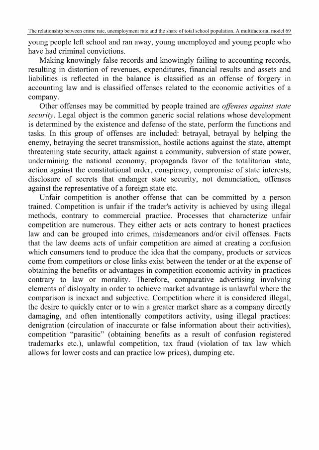
Evolution of unemployment rate in the period 1990-2010 in Bucharest

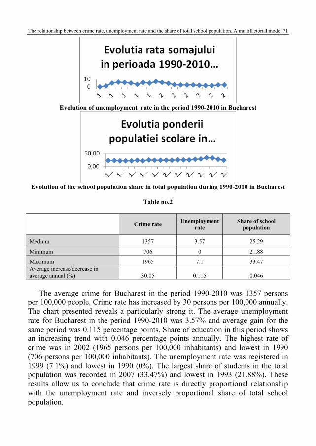
Evolution of the school population share in total population during 1990-2010 in Bucharest

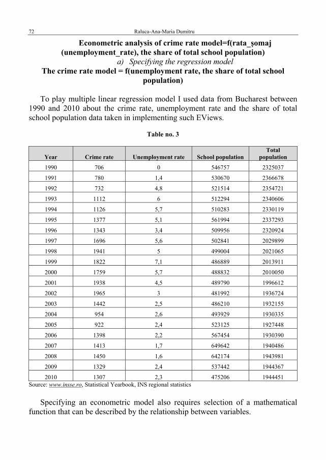
Table no.2

Crime rate

Unemployment rate

Share of school population

Medium 1357 3.57 25.29

Minimum 706 0 21.88

Maximum 1965 7.1 33.47 Average increase/decrease in average annual (%) 30.05 0.115 0.046

The average crime for Bucharest in the period 1990-2010 was 1357 persons

per 100,000 people. Crime rate has increased by 30 persons per 100,000 annually. The chart presented reveals a particularly strong it. The average unemployment rate for Bucharest in the period 1990-2010 was 3.57% and average gain for the same period was 0.115 percentage points. Share of education in this period shows an increasing trend with 0.046 percentage points annually. The highest rate of crime was in 2002 (1965 persons per 100,000 inhabitants) and lowest in 1990 (706 persons per 100,000 inhabitants). The unemployment rate was registered in 1999 (7.1%) and lowest in 1990 (0%). The largest share of students in the total population was recorded in 2007 (33.47%) and lowest in 1993 (21.88%). These results allow us to conclude that crime rate is directly proportional relationship with the unemployment rate and inversely proportional share of total school population.


Econometric analysis of crime rate model=f(rata_şomaj (unemployment_rate), the share of total school population)

a) Specifying the regression model The crime rate model = f(unemployment rate, the share of total school

population)

To play multiple linear regression model I used data from Bucharest between 1990 and 2010 about the crime rate, unemployment rate and the share of total school population data taken in implementing such EViews.

Table no. 3

Year Crime rate Unemployment rate School population Total

population

1990 706 0 546757 2325037

1991 780 1,4 530670 2366678

1992 732 4,8 521514 2354721

1993 1112 6 512294 2340606

1994 1126 5,7 510283 2330119

1995 1377 5,1 561994 2337293

1996 1343 3,4 509956 2320924

1997 1696 5,6 502841 2029899

1998 1941 5 499004 2021065

1999 1822 7,1 486889 2013911

2000 1759 5,7 488832 2010050

2001 1938 4,5 489790 1996612

2002 1965 3 481992 1936724

2003 1442 2,5 486210 1932155

2004 954 2,6 493929 1930335

2005 922 2,4 523125 1927448

2006 1398 2,2 567454 1930390

2007 1413 1,7 649642 1940486

2008 1450 1,6 642174 1943981

2009 1329 2,4 537442 1944367

2010 1307 2,3 475206 1944451 Source: www.insse.ro, Statistical Yearbook, INS regional statistics

Specifying an econometric model also requires selection of a mathematical

function that can be described by the relationship between variables.


Form multiple linear regression model is:

tttt scolarepopPondsomajRatatăăţiracţacţionRata εββα +++= __*_*inf_ 21

; t=1,2,…,n, where n=21

b) Estimate the regression model parameters multifactorial

Following parameter estimation in EViews equation is obtained: LS

Rata_infracţionalităţii=C(1)+C(2)*Rata_somaj+C(3)*Pond_pop_scolare The results are summarized below:

Estimation Command: ===================== LS RATA_INFRACT=C(1)+C(2)*RATA_SOMAJ+C(3)*POND_POP_SCOLARE Estimation Equation: ===================== RATA_INFRACT=C(1)+C(2)*RATA_SOMAJ+C(3)*POND_POP_SCOLARE Substituted Coefficients: ===================== RATA_INFRACT=599.664378+136.7541009*RATA_SOMAJ+58.07849829*POND_POP_SCOLARE

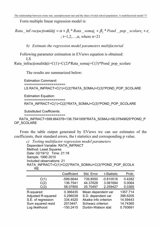
From the table output generated by EViews we can see estimates of the

coefficients, their standard errors, the t statistics and corresponding p value.

c) Testing multifactor regression model parameters Dependent Variable: RATA_INFRACT Method: Least Squares Date: 02/19/12 Time: 21:18 Sample: 1990 2010 Included observations: 21 RATA_INFRACT=C(1)+C(2)*RATA_SOMAJ+C(3)*POND_POP_SCOLA RE

Coefficient Std. Error t-Statistic Prob.

C(1) -599.6644 739.8550 -0.810516 0.4282 C(2) 136.7541 44.37628 3.081694 0.0064 C(3) 58.07850 25.70497 2.259427 0.0365

R-squared 0.366435 Mean dependent var 1357.714 Adjusted R-squared 0.296039 S.D. dependent var 398.6205 S.E. of regression 334.4520 Akaike info criterion 14.59443 Sum squared resid 2013447. Schwarz criterion 14.74365 Log likelihood -150.2415 Durbin-Watson stat 0.793691


If the crime rate increased by 1,000 persons per 100,000 population, the unemployment rate will increase by 136.75% and the share of total school population will increase by 58.07%.

3. Student Test

We have the hypotheses:

Null hypothesis, 0H : α = 0 or tβ = 0, t = 1,2

Alternative hypothesis, 1H : ≠α 0 or ≠tβ 0, t = 1,2

Thus the unemployment coefficient regression model is 1

∧β = 136.75,

standard error )( 1

∧βSE = 44.37 and statistics 1̂t = 3.08, calculates as

ErrorStd

tCoefficien

SEt

.)ˆ(

ˆˆ

1

11 ==

ββ

; p-value (p value) = 0.006, which shows that

unemployment is an important factor influencing the crime rate. Weight ratio of the school population in total population is =2β̂ 58.07,

standard error =)ˆ( 2βSE 25.7 and statistics 2̂t = 2.25. The probability is here 0.036, hence the share of total school population is a significant component of the crime rate regression model estimated.

Coefficient constant term in the regression model is ∧α =-559.66, standard

error )(∧αSE =739.85, t statistics expressed α

∧t = -0.81 with probability p value of

0.42. So free time is not significant for regression model chosen. The report of determination ( 2R ) shows what percentage is explained by the

influence of significant factors. It is calculated as: SSTSST

SSRR t

2

2 1−==

ε

. It is

used in assessing model quality. It can take only values in the range [0,1]. The values are closer to value 1, the model is better. The value that you take here is 0.3664 and thus we can say that the regression model is not very good. Approximately 36.64% the crime rate is explained by multiple linear regression model chosen.

scolarepoppondsomajrataitatiractionaliRata t __*ˆ_*ˆˆînf_ 21 ββα ++= ttt scolarepoppondsomajrataitatiractionaliRata __*07.58_*75.13666.599înf_ ++−=


-800

-400

0

400

800

400

800

1200

1600

2000

90 92 94 96 98 00 02 04 06 08 10

Residual Actual Fitted

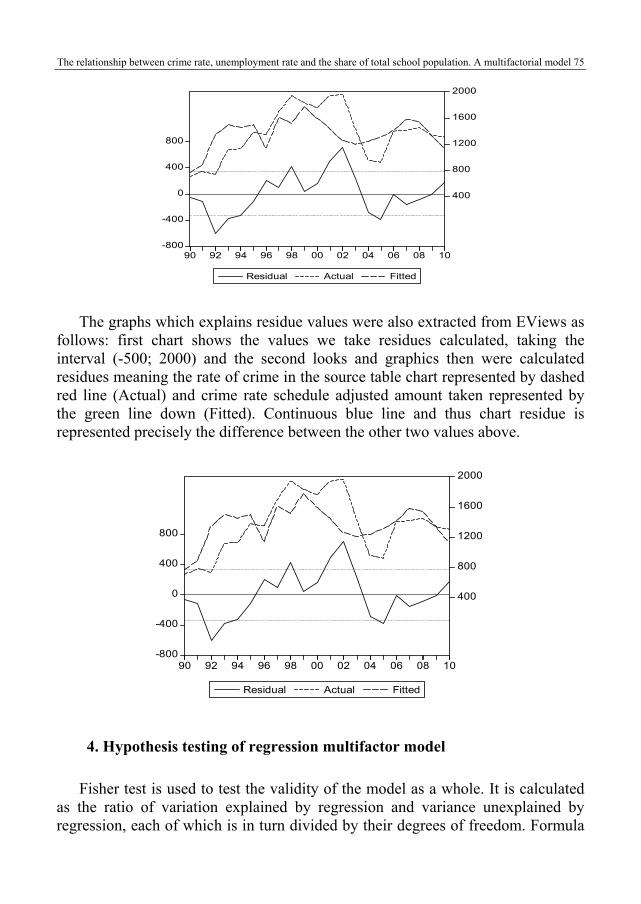
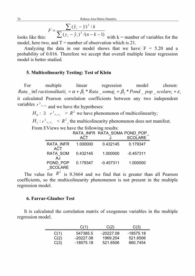
The graphs which explains residue values were also extracted from EViews as follows: first chart shows the values we take residues calculated, taking the interval (-500; 2000) and the second looks and graphics then were calculated residues meaning the rate of crime in the source table chart represented by dashed red line (Actual) and crime rate schedule adjusted amount taken represented by the green line down (Fitted). Continuous blue line and thus chart residue is represented precisely the difference between the other two values above.

-800

-400

0

400

800

400

800

1200

1600

2000

90 92 94 96 98 00 02 04 06 08 10

Residual Actual Fitted

4. Hypothesis testing of regression multifactor model

Fisher test is used to test the validity of the model as a whole. It is calculated as the ratio of variation explained by regression and variance unexplained by regression, each of which is in turn divided by their degrees of freedom. Formula


looks like this:

−−−−

=)1/()ˆ(

/)ˆ(2

2

knyy

kyyF

ii

i

with k = number of variables for the model, here two, and T = number of observation which is 21.

Analyzing the data in our model shows that we have F = 5.20 and a probability of 0.016. Therefore we accept that overall multiple linear regression model is better studied.

5. Multicolinearity Testing: Test of Klein

For multiple linear regression model chosen:

tttt scolarepopPondsomajRatatatiiractionaliRata εββα +++= __*_*inf_ 21

it calculated Pearson correlation coefficients between any two independent variables

ji xxr ,2

and we have the hypotheses:

:0H ∃ ji xxr ,

2 > 2R we have phenomenon of multicolinearity;

:1Hji xxr ,

2 < 2R , the multicolinearity phenomenon does not manifest.

From EViews we have the following results: RATA_INFR

ACT RATA_SOMA

J POND_POP_

SCOLARE

RATA_INFRACT

1.000000 0.432145 0.179347

RATA_SOMAJ

0.432145 1.000000 -0.457311

POND_POP_SCOLARE

0.179347 -0.457311 1.000000

The value for 2R is 0.3664 and we find that is greater than all Pearson

coefficients, so the multicolinearity phenomenon is not present in the multiple regression model.

6. Farrar-Glauber Test

It is calculated the correlation matrix of exogenous variables in the multiple regression model.

C(1) C(2) C(3)

C(1) 547385.5 -20227.08 -18575.18 C(2) -20227.08 1969.254 521.6506 C(3) -18575.18 521.6506 660.7454


0H : there is not the multicolinearity phenomenon

1H : is less than 1, there is multicolinearity phenomenon.

Test statistic will be equal with -414.92. It will compare with χ2

2

)1(;

−kkα =3.84.

Because the calculated value is less than the table shows that multicolinearity phenomenon can be neglected.

Checking normality: To test whether or not errors model follows a normal distribution will Jarque-

Bera test used with the following assumptions:

0H : errors follow a normal distribution: skewness = 0 and kurtosis = 3

1H : errors do not follow a normal distribution. It is known that if the errors are normal law of zero mean and mean square

deviation, then we have the relationship: ( ) αε εα −=≤ 1ˆ ˆstP i

Checking the assumption of normality of errors will be using Jarque-Berra test1 which is also an asymptotic test (valid for a large sample), which follows a chi-square distribution with a number of degrees of freedom equal to 2, the following form:

( )

−+=24

3

6

22 KSnJB ~ χ 3;α

where n = number of observations; S = coefficient of asymmetry (skewness), which measures the symmetry of

their distribution around the average error, which is equal to zero as the calculation the following relation:

( )3

1

31

σ

=

−=

n

ii yy

nS

K = coefficient of flattening calculated Pearson (kurtosis), which measures arching distribution (how “sharp” or flattened distribution is compared with the normal distribution), with the following equation for calculating:

( )4

1

41

σ

=

−=

n

ii yy

nK

1 EViews, User Guide,Version 2.0, QMS Quantitative Micro Software, Irvine, California, 1995, p. 140-141.


Jarque-Berra test assumes that the normal distribution has a zero asymmetry coefficient, S = 0, and a flattening coefficient equal to three, K = 3. If the probability p (JB) corresponding calculated value of the test is sufficiently low, then the assumption of normality of error is rejected, while otherwise, for a sufficiently high probability of error normality hypothesis is accepted or if >JB χ 2

2;α , then the hypothesis of normality of error is rejected.

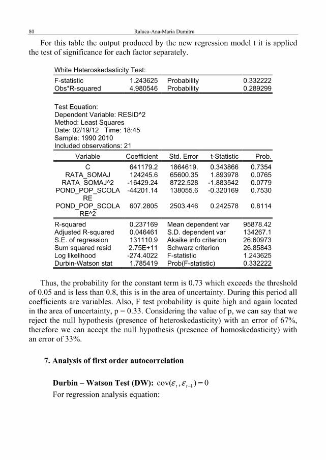
The JB test is 0.31. Note that Skewness = 1.00 and kurtosis = 3.18, probability of detection is =

0.85. Therefore we accept the null hypothesis, namely that it follows a normal distribution regression. This is observed with the schedule generated by EViews.

0

1

2

3

4

5

6

7

8

-750 -500 -250 0 250 500 750

Series: ResidualsSample 1990 2010Observations 21

Mean -6.90E-14Median -10.70249Maximum 708.8283Minimum -611.1940Std. Dev. 317.2891Skewness 0.290593Kurtosis 2.867705

Jarque-Bera 0.310870Probability 0.856043

Checking the homoskedasticity

The homoskedasticity refers to the hypothesis that the regression model that states that errors must have the same variance model: 2)( σε =tVar for any

t=1,...,n. Presence or not homoskedasticity can identify both graphically and using statistical tests. The chart residues certainly can not say no homoskedasticity existence, but also not the heteroskedasticity. Random variable (residual) is the medium void ( ) 0ˆ =εM and its dispersion

2ε̂s is constant and independent by X -

homoskedasticity hypothesis on which one can accept that the relationship between Y and X is relatively stable.

Error checking homoskedasticity hypothesis for this model will be using White test.

White-test involves the following steps:


- initial model parameter estimation and calculation of estimated residual variable, u;

- construct an auxiliary regression based on suppose of a relationship of dependency between the square error values, exogenous variables included in the initial model and the square of its values:

iii ixx ωαααε +++= 2

2102ˆ

and calculating the coefficient of determination, R2, corresponding to the

auxiliary regression; - verification of model parameters newly constructed meaning and one of them

is insignificant, then the error heteroskedasticity hypothesis is accepted. There are two versions of the test strip White:

- Fisher-Snedecor test using classic, based on the assumption invalid parameters, namely:

H0: 0210 === ααα

If the null hypothesis that the estimation results are insignificant (21 ;; vvc FF α< )

is accepted, then the homoskedasticity hypothesis is verified, the other case signified the presence of errors heteroskedasticity.

- use test LM (Lagrange multiplier), calculated as the number of observations corresponding to the n model and coefficient of determination, R2, corresponding to the auxiliary regressions. In general, the LM test is asymptotically distributed

as χ 2;vα , for the number of degrees of freedom is equal to: kv = , where k =

number of exogenous variables respectively: 2RnLM ⋅= ~ χ 2

;vα If >LM χ 2

;vα , errors are heteroscedastic, otherwise are homoscedastic, that

hypothesis of invalid parameters 0210 === ααα is accepted.

The most famous test is White’s test to test the following hypotheses:

Null hypothesis: 0H :22 σσ =i for all i =1,...,n

Alternative hypothesis 1H : 22 σσ ≠i for at least an i index.

More specifically, the initial regression model was built auxiliary regression:

it vscolarepoppondsomajratascolarapoppondsomajrata +++++= 25

23210

2 __*_*__*_* αααααε

The new errors vi are normally distributed and independent by iε .

In these circumstances you have the null hypothesis 0H : 0... 510 ==== ααα with the alternative 1H : not all parameters α are zero. If we

accept the null hypothesis, then we accept hypothesis homoskedasticity and if heteroskedasticity accept different parameters to 0.


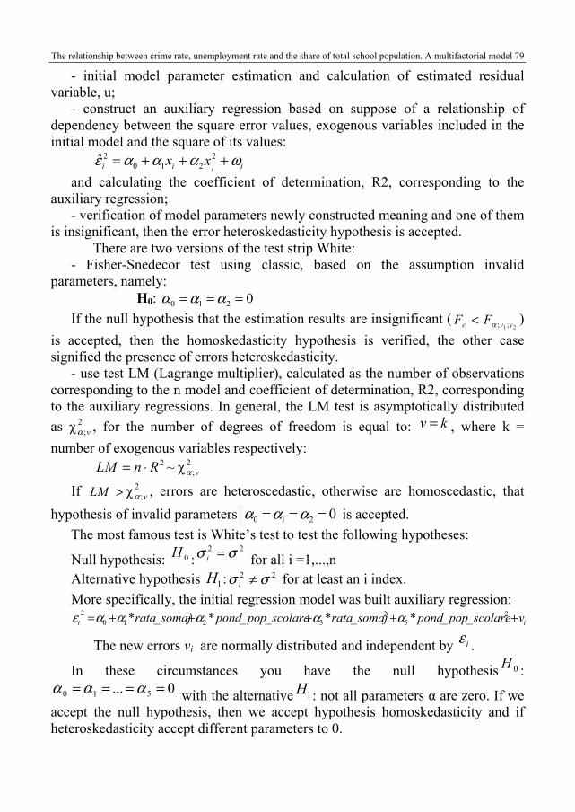
For this table the output produced by the new regression model t it is applied the test of significance for each factor separately.

White Heteroskedasticity Test:

F-statistic 1.243625 Probability 0.332222 Obs*R-squared 4.980546 Probability 0.289299

Test Equation: Dependent Variable: RESID^2 Method: Least Squares Date: 02/19/12 Time: 18:45 Sample: 1990 2010 Included observations: 21

Variable Coefficient Std. Error t-Statistic Prob.

C 641179.2 1864619. 0.343866 0.7354 RATA_SOMAJ 124245.6 65600.35 1.893978 0.0765

RATA_SOMAJ^2 -16429.24 8722.528 -1.883542 0.0779 POND_POP_SCOLA

RE -44201.14 138055.6 -0.320169 0.7530

POND_POP_SCOLARE^2

607.2805 2503.446 0.242578 0.8114

R-squared 0.237169 Mean dependent var 95878.42 Adjusted R-squared 0.046461 S.D. dependent var 134267.1 S.E. of regression 131110.9 Akaike info criterion 26.60973 Sum squared resid 2.75E+11 Schwarz criterion 26.85843 Log likelihood -274.4022 F-statistic 1.243625 Durbin-Watson stat 1.785419 Prob(F-statistic) 0.332222

Thus, the probability for the constant term is 0.73 which exceeds the threshold

of 0.05 and is less than 0.8, this is in the area of uncertainty. During this period all coefficients are variables. Also, F test probability is quite high and again located in the area of uncertainty, p = 0.33. Considering the value of p, we can say that we reject the null hypothesis (presence of heteroskedasticity) with an error of 67%, therefore we can accept the null hypothesis (presence of homoskedasticity) with an error of 33%.

7. Analysis of first order autocorrelation

Durbin – Watson Test (DW): 0),cov( 1 =−tt εε For regression analysis equation:


tttt scolarepopPondsomajRataitatiractionaliRata εββα +++= __*_*înf_ 21

I order autocorrelation of the error is expressed by the equation: ttt v+= −1ρεε

for t=2,...,n where tv ~N(0,

2tσ ). DW statistical test used pair of assumptions:

0H : ρ = 0 (null hypothesis); 1H : 0≠ρ (alternative hypothesis).

DW statistic is tabulated, values depending on the specified significance level, the number of observations in the sample and the number of variables influence the regression model. This, for a specified significance level, has two critical values is obtained from tables DW, 1d and 2d .

Reject the null hypothesis regions are defined as: If )4,( 22 ddDW −∈ , it is not autocorrelation;

If ),0( 1dDW ∈ , we have positive autocorrelation of errors;

If )4,4( 1dDW −∈ , we have negative autocorrelation of errors;

But if the DW test value is the remaining intervals ),( 21 dd or )4,4( 12 dd −− , the test is not conclusive.

In the model analyzed, statistics DW= 0.79. For a significance level of 5% of 21 observations and three variables influence the statistics tabulated values are:

=1d 1.13 and =2d 1.54. The value obtained in the model belongs to the

interval ),0( 1d , so errors are auto correlated positive.

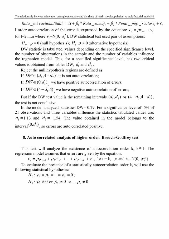
8. Auto correlated analysis of higher order: Breuch-Godfrey test

This test will analyze the existence of autocorrelation order k, k ≠ 1. The regression model assumes that errors are given by the equation:

tktkttt v++++= −−− ερερερε ...2211 , for t = k,...,n and tv ~N(0, 2vσ )

To evaluate the presence of a statistically autocorrelation order k, will use the following statistical hypotheses:

0H : 0...21 ==== kρρρ ;

1H : 01 ≠ρ or 02 ≠ρ or ... 0≠sρ

82 Raluca-Ana-Maria Dumitru Breusch-Godfrey Serial Correlation LM Test:

F-statistic 5.217452 Probability 0.018011 Obs*R-squared 8.289532 Probability 0.015847

Test Equation: Dependent Variable: RESID Method: Least Squares Date: 02/20/12 Time: 18:51 Presample missing value lagged residuals set to zero.

Variable Coefficient Std. Error t-Statistic Prob.

C(1) 10.53621 613.3542 0.017178 0.9865 C(2) 1.058553 36.86366 0.028715 0.9774 C(3) -0.397865 21.28591 -0.018691 0.9853

RESID(-1) 0.747565 0.246118 3.037427 0.0078 RESID(-2) -0.236943 0.247522 -0.957260 0.3527

R-squared 0.394740 Mean dependent var -6.90E-14 Adjusted R-squared 0.243425 S.D. dependent var 317.2891 S.E. of regression 275.9823 Akaike info criterion 14.28281 Sum squared resid 1218660. Schwarz criterion 14.53150 Log likelihood -144.9695 Durbin-Watson stat 2.033096

It is noted that statistical probability F is 0018 (rather large), so it is present

autocorrelation of order 2. After analyzing the data entered in the multiple regression model to obtain

better results on homoskedasticity, error autocorrelation or normality model, several observations can be introduced to capture the links between them.

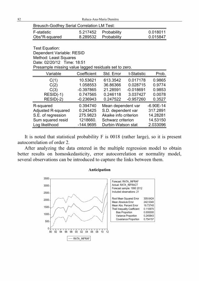
Anticipation

0

500

1000

1500

2000

2500

3000

3500

90 92 94 96 98 00 02 04 06 08 10 12

RATA_INFRAF

Forecast: RATA_INFRAFActual: RATA_INFRACTForecast sample: 1990 2012Included observations: 21

Root Mean Squared Error 309.6424Mean Absolute Error 242.5340Mean Abs. Percent Error 19.73745Theil Inequality Coefficient 0.110970 Bias Proportion 0.000000 Variance Proportion 0.245843 Covariance Proportion 0.754157


I supposed the unemployment rate for 2011 = 10% and 20% share of school and in 2012, unemployment 20% and 25% share of the school population and the forecast of the crime rate will be:

1990 766.3419 1991 893.9113 1992 1343.194 1993 1492.199 1994 1451.753 1995 1493.989 1996 1141.284 1997 1604.763 1998 1518.064 1999 1775.628 2000 1592.303 2001 1440.395 2002 1256.172 2003 1203.476 2004 1242.125 2005 1304.796 2006 1408.702 2007 1577.286 2008 1537.475 2009 1333.835 2010 1134.309 2011 2099.969 2012 2527.116

9. Conclusions

The multifactor model reflects the relationship between crime rate, unemployment rate and the share of total school population for the period 1990-2010 Bucharest is properly identified, have positive autocorrelation, so the model should be corrected. The data recorded by the INS on the economy of this county show that the crime rate is directly proportional to the unemployment rate and inversely proportional share of total school population. Analysis should be undertaken over several years, but must take into account the fact that in 2009 global economic crisis began.

Based on statements founder of sociology, E. Durkheim to say that is simply normal to have crime and that “any company that has the power to judge will inevitably use the power to punish”2, we can say that the prison institution, created in over two centuries ago is an indispensable component of the criminal justice system. However, it is clear that prison work around the world is still subject to extensive training process and to the consecration of other punitive state

2 Emile Durkheim, The rules of sociological method, Bucharest, Antet Publishing House, 2004, p.155


remains the main component that manages the execution of criminal punishment, deprivation of liberty.

Relative to prison work and approaches are extreme and contradictory. Thus, some criminologists and sociologists say that depth psychology have developed criminal and Penology, because it believes that virtually every human being can take potentially criminal behavior if circumstances lead him to such deeds, while others consider that the vast majority of adults, if not almost all people, commit over the course of life at least once criminal acts punishable by law.

However, other experts, including Gary Becker, Nobel laureate for economics in 1992, proposed the abolition of all prisons and custodial sentences replace all fine and its amount to cover the real cost of crime, which includes in addition amount of damage to victims and suppression costs resulting from criminal behavior, that financing costs for police, justice, etc. detention centers.

Perhaps to counter the current divergent it is noted internationally in recent years trying to redefine the role of justice in the community, fostering the application of alternative measures to detention and reduced role of the main prison and repressive element transformation to the community custodial institution.

Bibliography

1. Baltagi, B.H., Econometrics, New York, Springer, 2008 2. Bourbonnais, R., Terraza, M., Analyse des temporelles series, 3rd ed., Paris, Editions

DUNOD, 2010 3. Dorel, V., Action for unfair competition, Bucharest, Universitara Publishing House, 2011 4. Dumitru, M., Damages - interest in matters relating to trade, Bucharest, Hamangiu

Publishing House, 2008 5. Durbin, J., Watson, G.S., Testing for Serial Correlation in Least Squares Regression, in

Biometrika, vol. 38 (1951) 6. Durkheim, E., Rules of sociological method, Bucharest, Header Publishing House, 2004 7. Greene, W.H., Econometric Analysis, MIT Press Publishing House, 2002 8. Hayashi, F., Econometrics, Princeton University Press, 2000 9. Johnston, J., DiNardo, J.E., Econometric Methods, 4th ed., McGraw-Hill Publishing

House, 1997 10. Jula, D., Econometrics, Bucharest, Didactic and Pedagogic Publishing House, 2003 11. Jula, D., Introduction to Econometrics, Bucharest, Professional Consulting, 2003 12. Jula, N., Jula, D., Economic Modelling. Econometric Models and Optimization,

Bucharest, Mustang Publishing House, 2010 13. Lazăr, V., Unfair competition - Legal liability for anticompetitive practices in the

economic and commercial competition abusive acts were committed in Romania, Bucharest, Universitara Publishing House, 2008

14. Lazăr, V., Criminal Law - The Special (Offences under the Romanian Penal Code in force, as amended to date), Bucharest, Universitara Publishing House, 2006

15. Maddala, G.S., Introduction to Econometrics, 3rd ed., Wiley Publishing House, 2001


16. Maddala, G.S., Kim I.-M., Unit Roots, Cointegration and Structural Change, Cambridge University Press, 1999

17. Mukherjee, C., White, H., Wuyts, M., Econometrics and Data Analysis for Developing countries, Routledge, London and New York

18. Pecican, ES, Econometrics, Bucharest, All Publishing House, 1994 19. Pindyck, R.S., Rubinfeld, D.L., Econometric Models and Economic Forecasts, McGraw-

Hill Publishing House, 1991 20. Taşnadi, A., Applied Econometrics, Bucharest, ASE Publishing House, 2001 21. Thomas, R.L., Modern Econometrics: An Introduction, 2nd ed., Harlow, Longman, 1997 22. Tudorel, A., Econometrics, Bucharest, Economica Publishing House, 2008 23. Tudorel, A. (coord.), Introduction to Econometrics using EViews, Bucharest, Economica

Publishing House, 2008 24. Vangrevelinghe, G., Econometrics, Paris, Hermann Edition, 1973 25. Voineagu, V., Titan, E. Serban, R., Econometric Theory and Practice, Bucharest, Meteor

Press Publishing House, 2006 26. Wooldridge, J.M., Introductory Econometrics: A Modern Approach, 4th ed., Thomson

South-Western, 2009

Documents

ISSN THE RELATIONSHIP BETWEEN CRIME RATE, UNEMPLOYMENT ... · The relationship between crime rate, unemployment rate and the share of total school population. A multifactorial model