ISSUE PAPER ON - EPA Archives PAPER ON THE BIOAVAILABILITY ... 4.2.4 Adaptation and Acclimation ... bioaccessibility in terrestrial mammals

1

2

3

4

5

6

7

ISSUE PAPER ONTHE BIOAVAILABILITY

AND BIOACCUMULATIONOF METALS

DRAFT

John Drexler,1 Nicholas Fisher,2 Gerry Henningsen,3

Roman Lanno,4 Jim McGeer,5 Keith Sappington6

Contributing Author: Michael Beringer7

Submitted to:

U.S. Environmental Protection AgencyRisk Assessment Forum

1200 Pennsylvania Avenue, NWWashington, DC 20460 Contract #68-C-98-148

Submitted by:

ERG110 Hartwell AvenueLexington, MA 02421

August 2003

University of Colorado, Boulder, COState University of New York, Stony Brook, NYH&H Scientific Services, Centennial, COOhio State University, Columbus, OHNatural Resources Canada, Ottawa, ONNCEA, ORD, U.S. EPA, Washington, DCU.S. EPA Region 7, Kansas City, KS

ii

NOTICE

This paper has been developed in support of an ongoing effort within the U.S. EnvironmentalProtection Agency (EPA) to develop an integrated framework for metals risk assessment. InSeptember 2002, the cross-Agency technical panel, organized under the auspices of the Agency’sScience Policy Council, discussed plans for the development of the framework and associated guidancewith the Agency’s Science Advisory Board (SAB). During the advisory, the SAB affirmed theimportance of incorporating external input into the Agency’s effort. As part of the effort to engagestakeholders and the scientific community and to build on existing experience, the Agencycommissioned external experts to lead the development of papers on issues and state-of-the-artapproaches in metals risk assessment for several key topics. Topics identified include: environmentalchemistry; exposure; ecological effects; human health effects; and bioavailability and bioaccumulation.(Some individual EPA experts contributed specific discussions on topic(s) for which he or she haseither specific expertise or knowledge of current Agency practice). Although Agency technical staff, aswell as representatives from other Federal agencies, reviewed and commented on previous drafts, thecomments were addressed at the discretion of each respective author or group of authors. Therefore,the views expressed are those of the authors and should not be construed as implying EPA consent orendorsement.

This draft paper is being made available for public comment consistent with EPA’s commitmentto provide opportunities for external input. Science-based comments received on this paper will bemade available to authors for final disposition. The material contained in this paper may be used intotal, or in part, as source material for the Agency’s framework for metals risk assessment and EPA’sevaluation of this material will therefore include consideration of the Assessment Factors recentlypublished by EPA for use in evaluating the quality of scientific and technical information. The draftframework, as an Agency document, will undergo scientific peer review by the SAB.

Development of this draft paper was funded by EPA through its Risk Assessment Forum undercontract 68-C-98-148 to Eastern Research Group, Inc. Mention of trade names or commercialproducts does not constitute endorsement or recommendation for use.

TABLE OF CONTENTS

1. PROBLEM STATEMENT, CONCEPTUAL FRAMEWORK, AND DEFINITIONS ............ 11.1 Conceptual Framework ................................................................................................ 21.2 Definitions ................................................................................................................... 3

1.2.1 Bioaccessibility or Environmental Availability ............................................ 31.2.2 Bioavailability ............................................................................................... 31.2.3 Bioaccumulation ........................................................................................... 61.2.4 Other Definitions .......................................................................................... 7

2. PRINCIPLES ON BIOAVAILABILITY AND BIOACCUMULATION ................................ 72.1 Principles and Issues Common to Both Aquatic and Terrestrial Systems ................... 72.2 Membrane Interactions with Metals: Physicochemical Factors in Transfer of Metals

Across Membranes ................................................................................................. 92.2.1 Factors That Modify Absorption .................................................................. 9

2.3 Toxicokinetics (ADME) and Bioaccumulation of Metals ......................................... 10

3. CURRENT AGENCY PRACTICE ......................................................................................... 103.1 Site-Specific Assessments ......................................................................................... 10

3.1.1 Superfund Program ..................................................................................... 113.1.2 Ambient Water Quality Criteria ................................................................. 12

3.2 National-Scale Assessments ...................................................................................... 133.2.1 Assessing Health Risks of Lead Exposure ................................................. 133.2.2 Derivation of Reference Doses (RfDs) ...................................................... 133.2.3 National Risk Assessments ......................................................................... 143.2.4 National Criteria and Screening Levels ...................................................... 14

3.3 National Hazard Ranking and Classification ............................................................. 163.3.1 Toxics Release Inventory (TRI) ................................................................. 163.3.2 Waste Minimization Prioritization Tool ..................................................... 17

4. CURRENT STATE OF THE SCIENCE ON BIOACCUMULATION ANDBIOAVAILABILITY ISSUES ........................................................................................ 184.1 Aquatic ....................................................................................................................... 18

4.1.1 Aquatic Exposure ........................................................................................ 184.1.2 Dietary Exposure ........................................................................................ 19

4.2 Bioaccumulation of Metals in Aquatic Biota ............................................................ 204.2.1 Uptake Mechanisms .................................................................................... 204.2.2 Accumulation Strategy ............................................................................... 214.2.3 Trophic Transfer ......................................................................................... 234.2.4 Adaptation and Acclimation ....................................................................... 254.2.5 Intra/Intercellular Speciation ...................................................................... 264.2.6 Empirical Models/Methods ......................................................................... 274.2.7 Metabolism/Detoxification ......................................................................... 374.2.8 Biomonitoring as a Tool for Bioaccumulation ........................................... 39

4.3 Terrestrial ................................................................................................................... 40

iii

4.3.1 Human ......................................................................................................... 424.3.2 Wildlife ....................................................................................................... 504.3.3 Plants ........................................................................................................... 534.3.4 Soil Community: Invertebrates and Microorganisms ................................. 57

4.4 Speciation: Its Role in Assessing Bioavailability in the Terrestrial Environment .... 654.4.1 Speciation .................................................................................................... 664.4.2 Tools ........................................................................................................... 68

4.5 Predictive Assays for Terrestrial Mammals ............................................................... 70

5. FUTURE DIRECTIONS TO IMPROVE CURRENT AGENCY PRACTICE ...................... 765.1 Aquatic-Based Assessments ...................................................................................... 765.2 Research Needs .......................................................................................................... 87

5.2.1 Aquatic ....................................................................................................... 875.2.2 Terrestrial .................................................................................................... 87

6. LITERATURE CITED ............................................................................................................ 88

iv

LIST OF TABLES

Table 1. Mean concentration factors (on a wet weight or, for phytoplanktoncell volume basis) of metals in marine organisms............................................. 33

Table 2. Examples of relative bioavailability adjustments (RBA) inhuman health risk assessment............................................................................ 49

Table 3. Where bioavailability information is used in ecological risk assessment..........50

Table 4. Examples of including bioavailability processes in ecologicalrisk assessments.................................................................................................54

Table 5. Characteristics for direct speciation techniques................................................69

Table 6. Overall comparison of in vitro methods for metalbioaccessibility in terrestrial mammals.............................................................74

Table 7. Mean BCF/BAF as well as ACF values (with standarddeviation) for metals.........................................................................................81

Table 8. Regression coefficients (slope and intercept given with SEM)for the linear relationship of waterborne metal exposureconcentration and BCF value............................................................................82

LIST OF FIGURES

Figure 1. Conceptual diagram of processes controlling the bioavailabilityand bioaccumulation of metals in the environment............................................2

Figure 2. Conceptual diagram for evaluating bioavailability processes andbioaccessibility for metals in soil, sediment, or aquatic systems.......................4

Figure 3. Bioaccumulation factors for 42 different elements in Daphniamagna sampled from a natural source devoid of anthropogenic impact......... 31

Figure 4. Swine feeding studies using 17 field soils contaminated withlead and two laboratory-prepared soils............................................................ 47

Figure 5. Hypothetical conceptual model for direct and indirect exposureof ecological receptors to soil contaminants.....................................................51

Figure 6. Linkages between dietary toxicity threshold, bioaccumulationin prey organisms and waterborne exposure.....................................................84

v

1. PROBLEM STATEMENT, CONCEPTUAL FRAMEWORK, AND DEFINITIONS

The bioaccessibility, bioavailability, and bioaccumulation properties of inorganic metals in soil, sediments, and aquatic systems are complex. Similar to organic compounds, abiotic (e.g., organic carbon) and biotic (e.g., uptake and metabolism) modifying factors determine the amount of an inorganic metal that interacts at biological surfaces (e.g., at the gill, gut, or root-tip epithelium) and that binds to and is absorbed across these membranes. Metals are different from organic compounds in that they can be present as different species, with the parent element associating with different ligands, but never being irreversibly transformed or metabolized. To better characterize the risk presented by metals in the environment to human and ecological receptors, the processes that affect metal speciation and the effects of speciation on metal bioavailability must be understood and quantified to a greater degree. To evaluate the risk presented by metals, we must understand the influence of environmental characteristics on metal speciation as well as the speciation of metals within an organism. Once absorbed or assimilated into biota, metals are subject to a variety of fate processes including storage, metabolism, elimination, and accumulation.

Unlike organic xenobiotics, some metals are essential nutrients and can cause toxicity when not present in sufficient concentrations. However, excess amounts of certain metal species are potentially toxic when they interact with certain biomolecules in an organism. These features, along with the fact that metals persist as inorganic forms in environmental sinks (e.g., soil, sediments) and are cycled through the biotic components of an ecosystem, complicate evaluations of inorganic metal substances by adding complexity and uncertainty to hazard and risk assessments. The need to consistently and accurately measure quantitative differences in bioavailability between multiple forms of inorganic metals in the environment poses a major challenge for EPA. The need to understand metal bioaccumulation in relation to potential impacts also poses a major challenge for the Agency.

The goal of this paper is to summarize the current and emerging state of the science supporting assessments of metal bioavailability and bioaccumulation in aquatic and terrestrial organisms and, more importantly, to identify the relevance of this science for improving current Agency practices that involve (explicitly or implicitly) metals bioavailability and bioaccumulation. To accomplish this goal, we first introduce a conceptual model of the bioaccessibility, bioavailability, and bioaccumulation processes in relation to the expression of toxicity. Given the complex and overlapping nature of these concepts as well as the different definitions and uses of these terms in scientific literature, we define a number of related terms for the purposes of this paper.

These definitions are followed by sections addressing: (1) the principles and commonalities in metal physiology among organisms, (2) the state of the science supporting metals bioavailability and bioaccumulation assessments for aquatic and terrestrial receptors, (3) the current Agency practice for addressing metals bioavailability and bioaccumulation, and (4) recommendations for the future direction of Agency metals assessments and research needs.

1

Bioaccumulation etal mof

1.1 Conceptual Framework

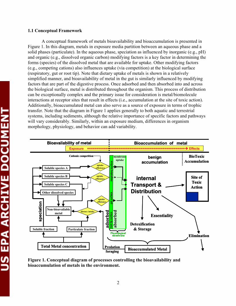
A conceptual framework of metals bioavailability and bioaccumulation is presented in Figure 1. In this diagram, metals in exposure media partition between an aqueous phase and a solid phases (particulate). In the aqueous phase, speciation as influenced by inorganic (e.g., pH) and organic (e.g., dissolved organic carbon) modifying factors is a key factor in determining the forms (species) of the dissolved metal that are available for uptake. Other modifying factors (e.g., competing cations) also influences uptake (via competition) at the biological surface (respiratory, gut or root tip). Note that dietary uptake of metals is shown in a relatively simplified manner, and bioavailability of metal in the gut is similarly influenced by modifying factors that are part of the digestive process. Once adsorbed and then absorbed into and across the biological surface, metal is distributed throughout the organism. This process of distribution can be exceptionally complex and the primary issue for consideration is metal/biomolecule interactions at receptor sites that result in effects (i.e., accumulation at the site of toxic action). Additionally, bioaccumulated metal can also serve as a source of exposure in terms of trophic transfer. Note that the diagram in Figure 1 applies generally to both aquatic and terrestrial systems, including sediments, although the relative importance of specific factors and pathways will vary considerably. Similarly, within an exposure medium, differences in organism morphology, physiology, and behavior can add variability.

Bioavailability of metal Bioavailability of metal Exposure =====================================================Î Effects

Bioaccumulation of metal

Total Metal concentration

BioToxic Accumulation

Site of Toxic Action

internal Transport & Distribution

spec

iat io

n

uptake efficiency

dietary intake

uptake efficiency

Bioaccumulated Metal

uptake efficiency

adso

rbed

Detoxification & Storage

Elimination

benign accumulation

Essentiality

Predation foraging

root

tip

surfa

ce

gut s

urfa

c e

resp

irato

r y s

urfa

c e

Cationic competition b e

Physiological membrane


Soluble fraction





Particulate fraction

Other dissolved species

Non-bioavailable metal

Soluble species A

Soluble species B

Soluble species C

spec

iat io

n

uptake efficiency

dietary intake

uptake efficiency


uptake efficiency

adso

rbed

abso

rbed


Elimination

benign accumulation

Essentiality

Predation foraging

root

tip

surfa

ce

gut s

urfa

c e

resp

irato

r y s

urfa

c e

Cationic competition membrane uptake


Figure 1. Conceptual diagram of processes controlling the bioavailability and bioaccumulation of metals in the environment.

2

1.2 Definitions

As broadly illustrated in Table 1-1 of the NRC document Bioavailability of Contaminants in Soils and Sediments: Processes, Tools, and Applications (NAS, 2002), many variations of terms and definitions are used for the concept of “bioavailability.” The NRC report does a good job of reviewing the history and nuances of the various terms and meanings involving “bioavailability processes.” However, the intention of this section and paper is to provide EPA with some practical, standard, and defensible recommendations on concepts, terms, and definitions that can serve as a paradigm for studying metals and their “bioavailability.” From this perspective, we propose that the following definitions might serve EPA risk assessors and risk managers best for their needs in addressing some of the myriad of problems involved with bioavailability and bioaccumulation of metals in the environment. Note that while definitions are often discussed in terms of both terrestrial as well as aquatic systems, some are more applicable to one media type than the other.

1.2.1 Bioaccessibility or Environmental Availability

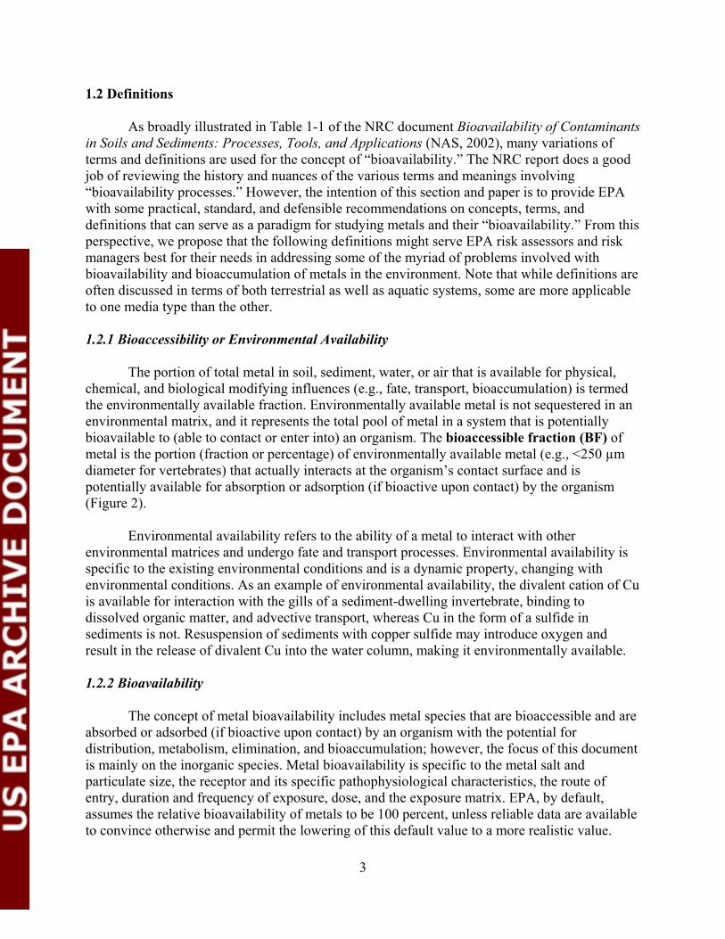
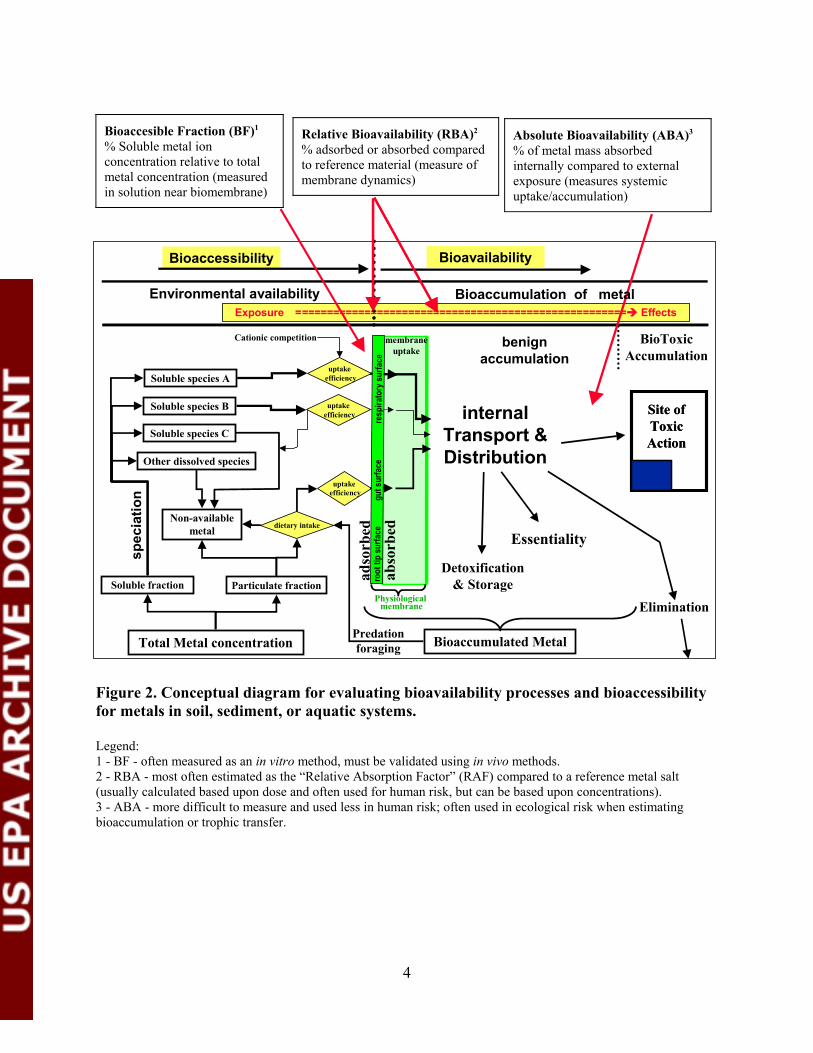
The portion of total metal in soil, sediment, water, or air that is available for physical, chemical, and biological modifying influences (e.g., fate, transport, bioaccumulation) is termed the environmentally available fraction. Environmentally available metal is not sequestered in an environmental matrix, and it represents the total pool of metal in a system that is potentially bioavailable to (able to contact or enter into) an organism. The bioaccessible fraction (BF) of metal is the portion (fraction or percentage) of environmentally available metal (e.g., <250 µm diameter for vertebrates) that actually interacts at the organism’s contact surface and is potentially available for absorption or adsorption (if bioactive upon contact) by the organism (Figure 2).

Environmental availability refers to the ability of a metal to interact with other environmental matrices and undergo fate and transport processes. Environmental availability is specific to the existing environmental conditions and is a dynamic property, changing with environmental conditions. As an example of environmental availability, the divalent cation of Cu is available for interaction with the gills of a sediment-dwelling invertebrate, binding to dissolved organic matter, and advective transport, whereas Cu in the form of a sulfide in sediments is not. Resuspension of sediments with copper sulfide may introduce oxygen and result in the release of divalent Cu into the water column, making it environmentally available.

1.2.2 Bioavailability

The concept of metal bioavailability includes metal species that are bioaccessible and are absorbed or adsorbed (if bioactive upon contact) by an organism with the potential for distribution, metabolism, elimination, and bioaccumulation; however, the focus of this document is mainly on the inorganic species. Metal bioavailability is specific to the metal salt and particulate size, the receptor and its specific pathophysiological characteristics, the route of entry, duration and frequency of exposure, dose, and the exposure matrix. EPA, by default, assumes the relative bioavailability of metals to be 100 percent, unless reliable data are available to convince otherwise and permit the lowering of this default value to a more realistic value.

3

Absolute Bioavailability (ABA)3

% of metal mass absorbed internally compared to external exposure (measures systemic uptake/accumulation)

Relative Bioavailability (RBA)2

% adsorbed or absorbed compared to reference material (measure of membrane dynamics)

Bioaccesible Fraction (BF)1

% Soluble metal ion concentration relative to total metal concentration (measured in solution near biomembrane)


Soluble fraction




Environmental availability


Particulate fraction

Other dissolved species

Non-available metal

Soluble species A

Soluble species B

Soluble species C

s pe c

iati o

n

uptake efficiency

dietary intake

uptake efficiency


uptake efficiency

adso

r be d

ab

sorb

ed


Bioaccumulation

Elimination

benign accumulation

Essentiality

Predation foraging

r oo t

t ip

sur fa

ce

g ut s

u rfa

ce

r es p

ir ato

ry s

u rfa

ce

Cationic competition

Bioaccessibility

membrane uptake


Exposure =====================================================Î Effects

Bioavailability

metal of

Figure 2. Conceptual diagram for evaluating bioavailability processes and bioaccessibility for metals in soil, sediment, or aquatic systems.

Legend:1 - BF - often measured as an in vitro method, must be validated using in vivo methods.2 - RBA - most often estimated as the “Relative Absorption Factor” (RAF) compared to a reference metal salt(usually calculated based upon dose and often used for human risk, but can be based upon concentrations).3 - ABA - more difficult to measure and used less in human risk; often used in ecological risk when estimatingbioaccumulation or trophic transfer.

4

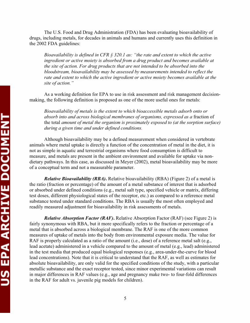
The U.S. Food and Drug Administration (FDA) has been evaluating bioavailability of drugs, including metals, for decades in animals and humans and currently uses this definition in the 2002 FDA guidelines:

Bioavailability is defined in CFR § 320.1 as: “the rate and extent to which the active ingredient or active moiety is absorbed from a drug product and becomes available at the site of action. For drug products that are not intended to be absorbed into the bloodstream, bioavailability may be assessed by measurements intended to reflect the rate and extent to which the active ingredient or active moiety becomes available at the site of action.”

As a working definition for EPA to use in risk assessment and risk management decision-making, the following definition is proposed as one of the more useful ones for metals:

Bioavailability of metals is the extent to which bioaccessible metals adsorb onto or absorb into and across biological membranes of organisms, expressed as a fraction of the total amount of metal the organism is proximately exposed to (at the sorption surface) during a given time and under defined conditions.

Although bioavailability may be a defined measurement when considered in vertebrate animals where metal uptake is directly a function of the concentration of metal in the diet, it is not as simple in aquatic and terrestrial organisms where food consumption is difficult to measure, and metals are present in the ambient environment and available for uptake via non-dietary pathways. In this case, as discussed in Meyer (2002), metal bioavailability may be more of a conceptual term and not a measurable parameter.

Relative Bioavailability (RBA). Relative bioavailability (RBA) (Figure 2) of a metal is the ratio (fraction or percentage) of the amount of a metal substance of interest that is adsorbed or absorbed under defined conditions (e.g., metal salt type, specified vehicle or matrix, differing test doses, different physiological states of the receptor, etc.) as compared to a reference metal substance tested under standard conditions. The RBA is usually the most often employed and readily measured adjustment for bioavailability in risk assessments of metals.

Relative Absorption Factor (RAF). Relative Absorption Factor (RAF) (see Figure 2) is fairly synonymous with RBA, but it more specifically refers to the fraction or percentage of a metal that is absorbed across a biological membrane. The RAF is one of the more common measures of uptake of metals into the body from environmental exposure media. The value for RAF is properly calculated as a ratio of the amount (i.e., dose) of a reference metal salt (e.g., lead acetate) administered in a vehicle compared to the amount of metal (e.g., lead) administered in the test media that produced equal biological responses (e.g., area-under-the-curve for blood lead concentrations). Note that it is critical to understand that the RAF, as well as estimates for absolute bioavailability, are only valid for the specified conditions of the study, with a particular metallic substance and the exact receptor tested, since minor experimental variations can result in major differences in RAF values (e.g., age and pregnancy make two- to four-fold differences in the RAF for adult vs. juvenile pig models for children).

5

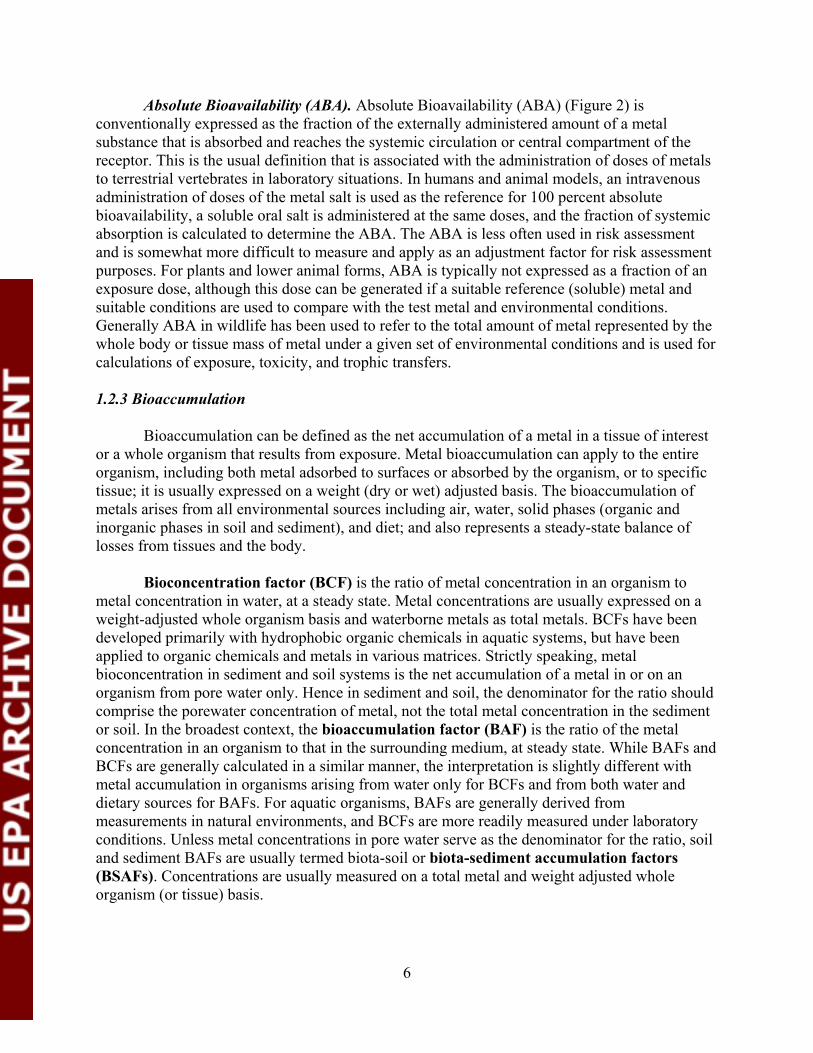
Absolute Bioavailability (ABA). Absolute Bioavailability (ABA) (Figure 2) is conventionally expressed as the fraction of the externally administered amount of a metal substance that is absorbed and reaches the systemic circulation or central compartment of the receptor. This is the usual definition that is associated with the administration of doses of metals to terrestrial vertebrates in laboratory situations. In humans and animal models, an intravenous administration of doses of the metal salt is used as the reference for 100 percent absolute bioavailability, a soluble oral salt is administered at the same doses, and the fraction of systemic absorption is calculated to determine the ABA. The ABA is less often used in risk assessment and is somewhat more difficult to measure and apply as an adjustment factor for risk assessment purposes. For plants and lower animal forms, ABA is typically not expressed as a fraction of an exposure dose, although this dose can be generated if a suitable reference (soluble) metal and suitable conditions are used to compare with the test metal and environmental conditions. Generally ABA in wildlife has been used to refer to the total amount of metal represented by the whole body or tissue mass of metal under a given set of environmental conditions and is used for calculations of exposure, toxicity, and trophic transfers.

1.2.3 Bioaccumulation

Bioaccumulation can be defined as the net accumulation of a metal in a tissue of interest or a whole organism that results from exposure. Metal bioaccumulation can apply to the entire organism, including both metal adsorbed to surfaces or absorbed by the organism, or to specific tissue; it is usually expressed on a weight (dry or wet) adjusted basis. The bioaccumulation of metals arises from all environmental sources including air, water, solid phases (organic and inorganic phases in soil and sediment), and diet; and also represents a steady-state balance of losses from tissues and the body.

Bioconcentration factor (BCF) is the ratio of metal concentration in an organism to metal concentration in water, at a steady state. Metal concentrations are usually expressed on a weight-adjusted whole organism basis and waterborne metals as total metals. BCFs have been developed primarily with hydrophobic organic chemicals in aquatic systems, but have been applied to organic chemicals and metals in various matrices. Strictly speaking, metal bioconcentration in sediment and soil systems is the net accumulation of a metal in or on an organism from pore water only. Hence in sediment and soil, the denominator for the ratio should comprise the porewater concentration of metal, not the total metal concentration in the sediment or soil. In the broadest context, the bioaccumulation factor (BAF) is the ratio of the metal concentration in an organism to that in the surrounding medium, at steady state. While BAFs and BCFs are generally calculated in a similar manner, the interpretation is slightly different with metal accumulation in organisms arising from water only for BCFs and from both water and dietary sources for BAFs. For aquatic organisms, BAFs are generally derived from measurements in natural environments, and BCFs are more readily measured under laboratory conditions. Unless metal concentrations in pore water serve as the denominator for the ratio, soil and sediment BAFs are usually termed biota-soil or biota-sediment accumulation factors (BSAFs). Concentrations are usually measured on a total metal and weight adjusted whole organism (or tissue) basis.

6

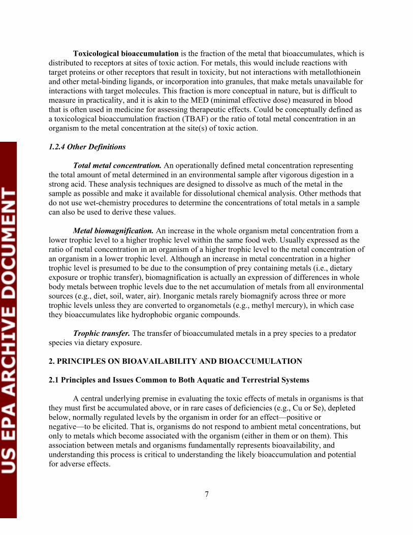
Toxicological bioaccumulation is the fraction of the metal that bioaccumulates, which is distributed to receptors at sites of toxic action. For metals, this would include reactions with target proteins or other receptors that result in toxicity, but not interactions with metallothionein and other metal-binding ligands, or incorporation into granules, that make metals unavailable for interactions with target molecules. This fraction is more conceptual in nature, but is difficult to measure in practicality, and it is akin to the MED (minimal effective dose) measured in blood that is often used in medicine for assessing therapeutic effects. Could be conceptually defined as a toxicological bioaccumulation fraction (TBAF) or the ratio of total metal concentration in an organism to the metal concentration at the site(s) of toxic action.

1.2.4 Other Definitions

Total metal concentration. An operationally defined metal concentration representing the total amount of metal determined in an environmental sample after vigorous digestion in a strong acid. These analysis techniques are designed to dissolve as much of the metal in the sample as possible and make it available for dissolutional chemical analysis. Other methods that do not use wet-chemistry procedures to determine the concentrations of total metals in a sample can also be used to derive these values.

Metal biomagnification. An increase in the whole organism metal concentration from a lower trophic level to a higher trophic level within the same food web. Usually expressed as the ratio of metal concentration in an organism of a higher trophic level to the metal concentration of an organism in a lower trophic level. Although an increase in metal concentration in a higher trophic level is presumed to be due to the consumption of prey containing metals (i.e., dietary exposure or trophic transfer), biomagnification is actually an expression of differences in whole body metals between trophic levels due to the net accumulation of metals from all environmental sources (e.g., diet, soil, water, air). Inorganic metals rarely biomagnify across three or more trophic levels unless they are converted to organometals (e.g., methyl mercury), in which case they bioaccumulates like hydrophobic organic compounds.

Trophic transfer. The transfer of bioaccumulated metals in a prey species to a predator species via dietary exposure.

2. PRINCIPLES ON BIOAVAILABILITY AND BIOACCUMULATION

2.1 Principles and Issues Common to Both Aquatic and Terrestrial Systems

A central underlying premise in evaluating the toxic effects of metals in organisms is that they must first be accumulated above, or in rare cases of deficiencies (e.g., Cu or Se), depleted below, normally regulated levels by the organism in order for an effect—positive or negative—to be elicited. That is, organisms do not respond to ambient metal concentrations, but only to metals which become associated with the organism (either in them or on them). This association between metals and organisms fundamentally represents bioavailability, and understanding this process is critical to understanding the likely bioaccumulation and potential for adverse effects.

7

Once absorbed by an organism, organic compounds may be metabolized, with the parent compound no longer present or decreasing over time in the organism. The metabolites or degradation products are usually less toxic than the parent compound, but, in some cases, they may become more toxic (e.g., carcinogenic PAHs). With metal compounds, there is no degradation of the metal atom itself, but the metal may bind to a wide variety of molecules in the organism. Metals can bind to biomolecules that are essential to cellular function (e.g., enzymes, structural proteins), alter their function, and cause toxicity. In some cases, metals bind to metallothioneins or phytochelatins, cysteine-rich compounds, or to other ligands that can help the organism regulate the metal within cells and detoxify the metal by preventing the binding to receptors that may result in toxicity. Metals may also be precipitated in phosphate or sulfide bodies within cells, thereby sequestering them and preventing mobility and subsequent toxicity. This issue has been reviewed by Mason and Jenkins (1995) and George (1990).

It is noteworthy that organisms have evolved in the presence of metals and in many cases have developed appropriate strategies of metal metabolism (homeostasis) when concentrations exceed those normally encountered by the organism. In contrast, most organic contaminants are typically novel compounds that have never been experienced during the evolutionary history of organisms; hence, they represent unique challenges to the organisms, as no specific sequestration or detoxification strategy has evolved—although several generic (oxidative and conjugative) metabolic pathways exist, which usually succeed in increasing the hydrophilicity of most organic compounds to facilitate elimination from the body. Many toxic metals become associated with sulfur-rich proteins, particularly Class B metals (e.g., Hg, Ag), whereas many organic contaminants of environmental concern (e.g., chlorinated hydrocarbons) are hydrophobic and, unlike metals, associate primarily with lipids in organisms.

The focus of these issue papers is on a subset of inorganic metals which generally behave in the manner of hydrophilic molecules described above. However, there are organometallic compounds (e.g., methylmercury, organoarsenicals) that have anthropogenic and dietary sources or are metabolites that are lipophilic. A feature that is unique to inorganic metals is that they persist. In contrast, when organic compounds (hydrocarbons) are mineralized to their basic elemental forms of carbon, hydrogen, and oxygen, they generally form relatively inert molecules of water or carbon dioxide which are considered GRAS substances (generally regarded as safe). In terms of both inorganic and organic forms of metals, it is the persistence of the bioavailable form of the metal which has most toxicological significance.

Another commonality exists for environmental inorganic metals, regardless of the receptor: the predominant exposure route of risk concern is oral for higher-order terrestrial receptors, while for aquatic receptors both respiratory and oral (dietary) route should be considered. The dermal route of inorganic metal uptake is usually a minimal contributor to exposure, due to the often effective barrier that most external epithelium provides to organisms. Exceptions include plants, where their root-tips and micro-environments resemble more the makeup of intestinal micro-villi with metal solution interfaces, and soft-bodied soil invertebrates (e.g., earthworms), where metal uptake is thought to occur primarily across the epidermis, which is also the respiratory surface. The message from this hierarchal observation is that it makes most sense to target research resources towards the evaluation of bioavailability at the species-specific biological membranes where most metal interactions and uptake occur (gut, gill, root-

8

tip). It should be an exceptional event to study respiratory (lung) and dermal (skin) bioavailability of inorganic metals in soils and sediment for vertebrates.

2.2 Membrane Interactions with Metals: Physicochemical Factors in Transfer of Metals Across Membranes (modified from Benet et al., 1996)

The absorption, distribution, and excretion of metals all involve passage across cell membranes. Therefore, it is essential to consider the mechanisms by which metals cross membranes and the physicochemical properties of metals and membranes that influence this transfer. Metals cross membranes either by passive processes or by mechanisms involving the active participation of components of the membrane. Most biological membranes are relatively permeable to water, either by diffusion or by flow that results from hydrostatic or osmotic differences across the membrane. Such bulk flow of water can carry with it small, water-soluble substances such as water and urea. While most inorganic ions would seem to be sufficiently small to penetrate the membrane, their hydrated ionic radius is relatively large. The concentration gradient of many inorganic ions is largely determined by active transport (e.g., Na+ and K+). The characteristics of active transport “selectivity, competitive inhibition by congeners, a requirement for energy, saturability, and movement against an electrochemical gradient” may be important in the mechanism of action of metals that are subject to active transport or that interfere with the active transport of essential minerals. An example would be lead which, because of properties similar to calcium, is taken up via calcium uptake mechanisms. The term facilitated diffusion describes a carrier-mediated transport process to which there is no input of energy, and movement of the substance in question thus cannot occur against an electrochemical gradient.

Absorption of metals involves mostly soluble metal ions, but it can also occur via endocytosis of metal particulates by cellular extrusions that engulf small particles and internalize them into the cytoplasm of the absorptive cell.

2.2.1 Factors That Modify Absorption

Many variables, in addition to the physicochemical factors that affect transport across membranes, influence the absorption of substances, including metals. Absorption, regardless of the site, is dependent upon solubility. Drugs given in aqueous solution are more rapidly absorbed than those given in oily solution, suspension, or solid form, because they mix more readily with the aqueous phase at the absorptive site. For those given in solid form, the rate of dissolution may be the limiting factor in their absorption. Local conditions at the site of absorption alter solubility, particularly in the gastrointestinal tract. The concentration influences its rate of absorption, as substances introduced at an administration site in solutions of high concentration are absorbed more rapidly than in solutions of low concentration. The circulation to the site of absorption also affects absorption. Increased blood flow, brought about by massage or local application of heat, enhances the rate of absorption; decreased blood flow, produced by vasoconstrictor agents, shock, or other disease factors, can slow absorption. The area of the absorbing surface to which a drug is exposed is one of the more important determinants of the rate of absorption. Drugs are absorbed very rapidly from large surface areas such as the

9

pulmonary alveolar epithelium and the intestinal mucosa (which can have an absorptive surface area of nearly two acres in humans).

2.3 Toxicokinetics (ADME) and Bioaccumulation of Metals

Toxicokinetics refers to the absorption, distribution, metabolism, and elimination (ADME) of toxicants. These four biological processes describe how most organisms process metals to which they are exposed and assimilate. Depending on the relative rates of uptake and elimination, a metal may accumulate to a steady-state level in different body compartments (e.g., tissues, organelles) that have varying affinities for the metal. There is usually a rate-limiting step that determines the steady-state level of metal in a tissue or receptor. Absorption controls the uptake of metal into the organism, and it is distributed to various areas depending upon the properties of the metal (e.g., elemental mercury distributes to the brain while inorganic ionic mercury has an affinity for kidney tissue) and the varying affinities of cells and biomolecules (e.g., red blood cells and brain purkingie cells in the cerebellum have a high affinity for methylmercury, while arsenic has an affinity for cysteine moieties on proteins). Some metals undergo limited metabolism, either by removing a bound substance (demethylation of organometallics) or by conjugating (methylation of arsenic) the metal. This would be particularly relevant to terrestrial organisms, where elimination generally occurs via the urine or equivalent if the metal form is ionic and water soluble, or via the feces if it is processed through the bile. Toxicokinetically, if the net-balance of uptake exceeds elimination for a metal, then bioaccumulation can occur, such as when a metal has a high affinity for tissues that can act as a reservoir, as with lead in bone tissue that has high calcium contents with which lead can interact (Weis et al., 1996; WHO, 1995). Toxicokinetics and the importance of the role of various ADME features varies with organism complexity.

3. CURRENT AGENCY PRACTICE

In this section, we summarize various methods EPA uses to incorporate metals bioavailability and bioaccumulation information into its regulatory programs. This discussion is not intended to be exhaustive in terms of the number of methods the Agency uses to address bioavailability or bioaccumulation nor in the detail provided for each method. Rather, its purpose is to provide the reader with some regulatory context on how EPA addresses the bioavailability and bioaccumulation of metals across a broad spectrum of regulatory programs. We have organized this discussion according to major “categories” of Agency assessments (e.g., site-specific assessment, national-scale assessment, national hazard ranking and classification). While this is not a formal classification scheme, it nonetheless serves to illustrate how the geographic scale and goal of the assessment influence how bioavailability and bioaccumulation information are considered in Agency metals assessments.

3.1 Site-Specific Assessments

Relative to national scale assessments, site-specific assessments are conceptually advantageous for incorporating bioavailability and bioaccumulation information, because factors that affect bioavailability and bioaccumulation can be measured directly (or indirectly) at the site of interest. However, this potential advantage can be tempered by difficulties resulting from gaps

10

11

in our knowledge of metals bioavailability and bioaccumulation processes, limitations inavailable resources to gather site-specific data, and spatial and temporal heterogeneity in metalsbioavailability and bioaccumulation within a site. The following discussion illustrates how site-specific data on bioavailability and bioaccumulation are addressed by two Agency programs: theSuperfund and Ambient Water Quality Criteria programs.

3.1.1 Superfund Program

The Office of Solid Waste and Emergency Response (OSWER) is responsible foradministering the assessment and management of risks associated with hazardous sites listed onthe National Priorities List as part of the Superfund program, in addition to other functions. In1989, OSWER published Risk Assessment Guidance for Superfund (RAGS) Part A for use inhuman health risk assessments at Superfund sites (U.S. EPA, 1989a) and has since updated thisguidance periodically (U.S. EPA, 2001d). General guidance for making adjustments to ensureconsistent treatment of bioavailability assumptions in exposure and toxicity is included asAppendix A in RAGS. This guidance recognizes the need to make adjustments to bioavailabilityassumptions to account for differences in absorption efficiencies between the medium ofexposure and the medium assumed by the toxicity value. It also discusses the need to adjust fordifferences in the expression of dose between the exposure and toxicity value (e.g., absorbedversus administered dose). In the absence of adequate data to the contrary, the RAGS guidancerecommends that the relative bioavailability of a chemical should be assumed to be equal infood, water, or soil. To date, the most common treatment of bioavailability for human healthassessments for all chemicals, including metals, is to assume that the bioavailability of the metalexposure on the site is the same as the bioavailability used to derive the toxicity value used toestimate risk. This is typically accomplished by relying on laboratory toxicity tests, whichusually measure administered rather than absorbed doses.

In some situations, site-specific adjustments of default bioavailability assumptions areconducted when sufficient data are available. Usually this entails conducting a well-designedanimal feeding study with juvenile swine which has been identified as the preferred animalmodel for lead (U.S. EPA, 1999a). This has been accomplished at several sites across thecountry including the Murray Smelter in CO; Palmerton, PA; Jasper County, MO; SmugglerMountain, CO; and the Kennecott site in Salt Lake City, UT. Although in vitro tests have beendeveloped for assessing bioavailability differences of lead in soils, the Agency currently requiresadditional validation of these approaches before they can be used as the sole basis for makingbioavailability adjustments (U.S. EPA, 1999a).

Interim draft guidance has also been developed by EPA Region 10 for makingbioavailability adjustments with arsenic contaminated soil (U.S. EPA, 2000a). Based onliterature data on arsenic bioavailability and the results of a Region 10 animal study in whichimmature swine were dosed with arsenic contaminated soil derived from the Ruston/NorthTacoma Superfund site that was a former smelter site (U.S. EPA, 1996a), this interim guidancerecommends default values of relative bioavailability for arsenic in soil ranging from 60 percentto 100 percent depending on the source of contamination (e.g., mineral processing, fossil fuelcombustion, pesticides/wood treatment processes). Similar to the case with lead, the juvenileswine is the recommended animal model for supporting departures from the default relative

12

bioavailability assumptions. Bioavailability data from in vitro studies are not recommended foruse as the sole basis for making relative bioavailability adjustments, but can be used to justifythe appropriateness of using in vivo data from other sites. In mid April, 2003, EPA convened aworkshop to address the use of bioavailability data in human health risk assessments atcontaminated sites (http://conference.syrres.com). EPA expects to use information presentedduring this workshop in its efforts to establish the most scientifically sound approach to utilizingbioavailability measurements for metals at contaminated sites.

Methods for assessing the existing condition of metals accumulation commonly involvemeasurement of metal residues in organisms at the study site. However, when bioaccumulationmust be predicted under future conditions, empirically-based bioaccumulation factors (indexedto water, soil, or sediment) or site-specific regression relationships can be used to quantify therelationship between exposure media and tissue residues. In the context of ecological riskassessments involving Superfund sites, EPA has published generalized criteria for designingfield studies with the intent of quantifying bioaccumulation factors (U.S. EPA, 1997a), althoughthis guidance is not specific to metals. Some examples of empirical approaches for quantifyingmetals bioaccumulation relationships at the site level have been described by Nan et al. (2002),Torres and Johnson (2001a), and Sample et al. (1999, 1998), although these are not necessarilyspecific to Superfund assessments. Mechanistic approaches such as bioenergetically orphysiologically based bioaccumulation models have been developed for metals, but they haveachieved mixed success in terms of their accuracy in predicting metals bioaccumulation (e.g.,Simas et al., 2001, for aquatic macrofauna; Saxe et al., 2001, for earthworms; Ke and Wang,2001, for oysters; and Goree et al., 1995, for cadmium). Application of mechanistically basedmodels in site-specific risk assessments (including Superfund assessments) is much less commondue to the resource demands needed to satisfy input data requirements and calibrate the modelsand their lack of widespread validation.

3.1.2 Ambient Water Quality Criteria

EPA’s Office of Water is charged with developing ambient water quality criteria(AWQC) to support the Clean Water Act goals of protecting and maintaining physical, chemical,and biological integrity of waters of the United States. Examples of chemical-specific criteriainclude those designed to protect human health, aquatic life, and wildlife. Although AWQC aretypically derived at a national level, there has been a long history behind the development ofmethods to accommodate site-specific differences in metals bioavailability. For example, sincethe 1980s aquatic life criteria for several cationic metals have been expressed as a function ofwater hardness to address the combined effect of certain cations (principally calcium andmagnesium) on toxicity. Recognizing that water hardness adjustments did not account for otherimportant ions and ligands that can alter metals bioavailability and toxicity, EPA developed theWater Effect Ratio (WER) procedure as an empirical approach for making site-specificbioavailability adjustments to criteria (U.S. EPA, 1994). This approach relies on comparingtoxicity measurements made in site water to those made in laboratory water to derive a WER.The WER is then used to adjust the national criterion to reflect site-specific bioavailability.

More recently, the Office of Water has been developing a mechanistic-based approachfor addressing metals bioavailability using the Biotic Ligand Model or BLM (U.S. EPA, 2000g;

13

DiToro et al., 2001; Santore et al., 2001). This model, which is described in further detail inSection 4, predicts acute toxicity to aquatic organisms based on physical and chemical factorsaffecting speciation, complexation, and competition of metals for interaction at the biotic ligand(i.e., the gill in the case of fish). The BLM has been most extensively developed for copper andis being incorporated directly into the national copper aquatic life criterion. The BLM is alsobeing developed for use with other metals including silver. Conceptually, the BLM hasregulatory appeal because metals criteria could be implemented to account for predicted periodsof enhanced bioavailability at a site which may not be captured by purely empirical methodssuch as the WER.

3.2 National-Scale Assessments

By their very nature, national regulatory assessments often lack the data necessary toincorporate many potentially important site-specific factors that can affect bioavailability andbioaccumulation. Due to complex issues, uncertainties, and data gaps associated withcharacterizing metals bioavailability, the application of bioavailability factors or mechanisticmodels in risk assessments is not a typical practice in most national-scale risk assessments.While it is commonly known that bioavailability of metals in the environment may besubstantially reduced by a number of factors (e.g., complexation, precipitation, competition withenvironmental ligands, sorption onto soils and sediments, formation of insoluble metalcompounds), screening risk assessments often assume the bioavailability of the species of metalin the assessment is the same as the bioavailability of the species of metal used to develop thetoxicity value. This occurs principally because of a lack of validated data and models forassessing/predicting gut absorption of ingested metal, dissolution of ingested metals, biotaspecific detoxification of metals, toxicity relationship between the metal forms tested in thelaboratory and metal forms ingested, and other assessment specific factors. These aspectscontribute to the challenges of conducting national-scale metal assessments. Several examples ofhow the Agency has addressed bioavailability and bioaccumulation issues in the context ofnational-scale assessments are summarized below.

3.2.1 Assessing Health Risks of Lead Exposure

For assessing risk associated with lead exposure in children, blood lead levels aretypically predicted using the Integrated Exposure Uptake Biokinetic Model for Lead in Children(IEUBK) developed by EPA (U.S. EPA, 2001a). For addressing differences in leadbioavailability in different environmental media, the IEUBK model assigns default values ofabsolute bioavailability to all lead exposure media. The default values for air, water, and soil are32 percent, 50 percent, and 30 percent, respectively (U.S. EPA, 2001b). For non-residentialscenarios, EPA has developed the Adult Lead Methodology which assumes the absolutebioavailability of lead in soil is 12 percent (U.S. EPA, 1996b).

3.2.2 Derivation of Reference Doses (RfDs)

The Agency also derives RfDs that are specific for an exposure medium based onconsideration of bioavailability or other factors that might suggest unique dose-responserelationships in that medium. For example, separate oral RfDs have been derived for cadmium in

14

food and drinking water based on the rationale that the bioavailability of cadmium in water isgreater than that of cadmium in food by a factor of 2 (i.e., 5 percent versus 2.5 percent,respectively) (U.S. EPA, 2003a). EPA has also recommended that a modifying factor of three beapplied to the chronic oral RfD for manganese when the RfD is used to assess risks fromdrinking water or soil to account, in part, for potential differences in bioavailability ofmanganese in water and soil compared to food (U.S. EPA, 2003b).

3.2.3 National Risk Assessments

As part of a national risk assessment of land applied sewage sludge, EPA relied almostexclusively on empirical data to address metals bioaccumulation from soil to plants (U.S. EPA,1995a). That is, data from a variety of soils were used—crops, cationic exchange capacities ofsoils, soil pH, soil organic carbon, and soil moisture. Therefore, overall bioavailability of metalsfrom soil to crops/vegetation was automatically integrated into the exposure assessment, but notthrough a mechanistic basis.

As part of a national risk assessment of atmospheric mercury releases, EPA relied onbioaccumulation factors to characterize mercury bioaccumulation in aquatic food webs (U.S.EPA, 1997b). Bioaccumulation factors derived from the scientific literature were expressed ascentral tendency estimates for each trophic level (e.g., trophic level one through fourrepresenting primary producers (phytoplankton, periphyton), herbivores, forage fish and toppredator fish, respectively). To address some aspects of mercury speciation and its effect onbioavailability, BAFs were expressed as a function of dissolved methylmercury in the watercolumn, which is considered to be the most bioavailable form of environmental mercury. Basedon this compilation of BAF data, considerable variability in methylmercury BAF data occurseven within a trophic level. A number of factors are thought to contribute to this variability,including site-specific differences in methylmercury bioavailability, variation in food webstructure among study locations, species-specific differences in accumulation rates, uncertaintyin assessing trophic position, and in the case of fish, variability in age of organisms used tocalculate BAFs. 3.2.4 National Criteria and Screening Levels

National ambient water quality criteria developed by EPA to protect human health andwildlife typically address bioaccumulation of chemicals (including metals) through the use ofBCFs and BAFs (U.S. EPA, 1995b, 2000c). For national AWQC derivation, geometric means ofBAFs and BCFs are determined within a specified trophic level account for possiblebiomagnification and broad physiological and ecological differences that can affectbioaccumulation. Because a BCF or BAF for a given chemical and organism will varydepending on the exposure duration up to the point where steady state is reached, BAF and BCFdata are screened by EPA to select those values which reflect longer-term accumulation in orderto approximate steady-state conditions. Since the protection goals of EPA water quality criteriaare known (i.e., protection of human health or wildlife), BAFs and BCFs are selected for speciesand tissues that are most relevant to human and wildlife exposure.

15

For deriving water quality criteria, the EPA has provided limited guidance for evaluatingBCFs and BAFs for metals in the context of issues associated with metals essentiality andconcentration dependency of BCFs and BAFs. For example, in situations where BCFs vary withexposure concentration, earlier guidance recommends using the BCF from the lowest exposureconcentration above the control treatment (U.S. EPA, 1985, 1995b). If the chemical is amicronutrient, this guidance recommends that concentrations of the inorganic chemical begreater than background levels and greater than levels required for normal nutrition of the testspecies. In cases of BCF (BAF) concentration dependency, EPA’s updated water quality criteriaguidance for the protection of human health further recommends using BCFs or BAFs fromconcentrations that most closely align with the water quality criterion (U.S. EPA, 2000c). Thisrecommendation attempts to minimize extrapolation of BAF or BCF values across widelydiffering water column concentrations that might result from differences in the exposureconcentration used in a BCF or BAF study, compared to the concentration associated with awater quality criterion. In theory, such an approach might use an allowable dietary intakeconcentration (determined from the toxicity and exposure data) and the concentration-tissueresidue relationship derived from the BCF or BAF study to identify the ambient concentrationthat is most suitable for estimating the BCF or BAF. However, this guidance has not yet beenapplied for deriving criteria.

Unlike the derivation of BCFs and BAFs nonionic organic chemicals which are adjustedto account for chemical partitioning into lipids of the organism and organic carbon in water,analogous procedures have yet to be developed for the derivation of BAFs and BCFs for metals.For deriving BAF and BCF values for use in human health ambient water quality criteria, EPAcurrently recommends that metals bioavailability be addressed on a metal-by-metal basis to theextent that data provide adequate justification for making broad-scale adjustments (U.S. EPA2000c).

Over the past decade, significant scientific advances have been made in addressingmetals bioavailability in sediments in relation to their toxicity to benthic organisms. In thederivation of sediment equilibrium partitioning benchmarks for mixtures of metals involvingcadmium, copper, lead, nickel, silver and zinc, EPA incorporates bioavailability through aprocedure that compares the concentration of amorphous sulfide ligands known as acid volatilesulfides (AVS) and the concentration of simultaneously extracted metals (SEM) from the AVSprocedure (U.S. EPA, 2002a). This approach is based on previous studies that demonstrate whenAVS is in excess of SEM on a molar basis, toxicity to benthic macroinvertebrates is notobserved due to the formation of insoluble metal sulfides, subsequently reducing metalconcentrations in sediment pore water (Ankley et al., 1994; Hansen et al., 1996; Berry et al,1999; Di Toro et al., 1992, 1990). As the excess of SEM over AVS increases, the probability ofobserving toxicity also increases, although the precise prediction of toxicity is somewhatuncertain when excess SEM is small. When SEM exceeds AVS, consideration of other ligands,especially total organic carbon, can reduce uncertainty in the prediction of toxicity.

For establishing national ecological screening levels of metals in soil, empirically basedsoil-to-biota bioaccumulation factors and regression models have been developed and applied(U.S. EPA, 2000d; Sample et al., 1999, 1998). Because variation in these factors and regressionmodels can be substantial across sites (spanning several orders of magnitude), conservative

estimates of soil-to-biota BAFs are being used in this screening application. In general, data for developing soil-to-biota accumulation factors are far more limited compared to aquatic-based BAFs and BCFs.

3.3 National Hazard Ranking and Classification

EPA uses national ranking and characterization procedures in a number of its regulatory programs, some of which include the Toxics Release Inventory (TRI) program, the Hazardous Waste Minimization program, and the New Chemicals (Premanufacture Notification program). The specific purpose of the various chemical ranking and classification procedures vary by program, but in general, they are designed to rank or classify large numbers of chemicals by selected attributes of interest (e.g., persistence, bioaccumulation, and toxicity) in order to establish priorities for future analysis, action or information notification.

In general, quantitative considerations of bioavailability are difficult with national hazard ranking and classification methods due to widely varying environmental conditions across the country, the need to be protective of many different types of organisms in different media, the lack of bioavailability data in organisms, and the increased uncertainty due to the broad scope of national hazard or risk characterizations. To be sufficiently protective, decisions about national hazard ranking and characterization assessments are usually driven by available toxicity data and whether there are environmental conditions within the United States that would cause a metal to become or remain available in the environment or favor formation of bioavailable forms of the metal. The treatment of bioavailability and bioaccumulation data in two hazard ranking and classification procedures used by EPA is summarized below.

3.3.1 Toxics Release Inventory (TRI)

Established under Section 313 of the Emergency Planning Community Right-to-Know Act (EPCRA), EPA’s Toxic Release Inventory (TRI) Program is responsible for collecting and disseminating information on the environmental releases and waste management activities of chemicals listed on the EPCRA Section 313 list of toxic chemicals. This program requires certain facilities to report annually to EPA on the release and waste management of chemicals above certain activity thresholds (e.g., 25,000 lbs or more for manufacturing/processing or 10,000 lbs for other uses). EPA’s TRI Program published a final rule in 1999 which focused on lowering the reporting thresholds for a group of chemicals classified as “Persistent, Bioaccumulative and Toxic” or PBT as a result of growing national and international concern over the potential for harmful exposure to these compounds (U.S. EPA, 1999b). Classifying compounds into the PBT category requires evaluation of data on persistence in various environmental media, bioaccumulation, and toxicity.

The “B” portion of the PBT classification under TRI requires evaluation of the magnitude and potential for compounds to bioaccumulate in organisms. This evaluation is primarily accomplished through the review and comparison of aquatic BCF and BAF data to established benchmarks (e.g., 1000 and 5000 for classifying compounds as “bioaccumulative” and “highly bioaccumulative,” respectively). However, as part of the TRI rule for lead and lead compounds, data on lead accumulation in humans were considered in addition to aquatic BCF

16

data for classifying lead as “bioaccumulative” (U.S. EPA, 2001c). Consideration of human data was largely qualitative because of the lack of formal procedures for comparing human bioaccumulation data to quantitative benchmarks. Given the broad assessment goals of the PBT classifications under the TRI program (i.e., ranking chemical hazard based on all relevant exposure pathways, environmental media, and ecological and human receptors), each aquatic species for which BCF or BAF data are available is considered equally for comparing to benchmark values (U.S. EPA, 2001c, 2000h). For example, in the final lead TRI rule, equal consideration was given to lead bioaccumulation in algal species versus data from other aquatic species (e.g., bivalves, fish, etc.) (U.S. EPA, 2001c).

The broad assessment goals of national hazard ranking and classification programs complicate the ability to incorporate bioavailability adjustments into the PBT classification procedure. When conducting hazard assessments of metals, information on environmental fate is reviewed to establish whether or not forms of metals can become bioavailable under wide ranging environmental conditions and potential exposure scenarios encountered at a national scale (U.S. EPA, 1991, 1999b). Since the bioaccumulation classification relies principally on aquatic BCF and BAF data, the bioavailability of a metal compound (or metal compounds within a given category) released to the environment is implicitly assumed to be representative of metal forms and conditions found in the applicable BCF and BAF studies (typically soluble metal salts in laboratory tests).

Regarding metals essentiality and inverse relationships between BCFs and exposure concentrations, similar guidance is followed for evaluating BCF and BAF data as discussed previously for deriving ambient water quality criteria (U.S. EPA, 2000h). However, the existence of inverse relationships between BCF (BAF) and exposure concentrations for certain metal/species combinations has led to recommendations by some to abandon the current use of BCFs and BAFs for classifying metal hazards (Adams, 2000; Brix and Deforest, 2000; McGeer et al., 2003). For comparative purposes, the OECD has recently published guidance for classifying metals that are hazardous to aquatic environments (OECD, 2001). The hazard classification schemes presented in the guidance incorporate, among other parameters, evidence of bioaccumulation (i.e., a BCF value greater than or equal to 500 in fish) as a basis for hazard ranking. The OECD guidance further acknowledges the complexities and variability associated with metals uptake and depuration and the existence of an inverse relationship between water concentration and BCF in some aquatic organisms. As a result, this guidance recommends that bioaccumulation data for metals be used with care and that metals bioaccumulation according to the classification criteria be conducted on a case-by-case basis.

3.3.2 Waste Minimization Prioritization Tool

The WMPT is a joint product of EPA’s Office of Solid Waste (OSW) and EPA’s Office of Pollution Prevention and Toxics (OPPT). It provides a screening-level assessment of potential chronic (i.e., long-term) risks to human health and the environment (U.S. EPA 2000e). Its overall purpose is to assist in the process of prioritizing chemicals for voluntary pollution prevention activities. The WMPT is a scoring system that was developed to rank chemicals based on their persistence (P), bioaccumulation potential (B), and human (HT) and ecological toxicity (ET). Chemicals are given a score of 1 (low concern), 2 (medium concern), or 3 (high

17

concern) for P, B, and HT or ET resulting in an overall PBT score between 3 and 9. Like the TRI PBT classification system, bioaccumulation is evaluated using BCF or BAF data. A score of 1 is assigned to BCF or BAF values less that 250; a score of 2 is assigned for BCF or BAF values from 250 to 1000; and a score of 3 is assigned for BCF or BAF values exceeding 1000. Evaluation of BCF and BAF data is similar to that discussed under the TRI PBT classification program. Originally, some metals were identified as priority chemicals for the OSW’s Waste Minimization Program based on their analysis using the PBT Framework within the WMPT. However, OSW has since deferred the use of that criterion for the identification of its Waste Minimization Priority Chemicals, because of EPA’s work with its Science Advisory Board to develop a consistent, Agency-wide approach (i.e., the Metals Assessment Framework) for the evaluation of metals. Regardless of those issues, other information was identified that clearly demonstrated that some metals should remain as priorities for OSW’s Waste Minimization Program.

4. CURRENT STATE OF THE SCIENCE ON BIOACCUMULATION AND BIOAVAILABILITY ISSUES

4.1 Aquatic

This discussion of the aquatic bioavailability and bioaccumulation of metals is a generalized discussion of the subject. It uses examples to illustrate some of the features of metal bioaccumulation and bioavailability and should not be considered as a comprehensive examination of the subject. Similarly it does not provide an inclusive discussion of all aquatic plant and animal species but exposure via aqueous systems. In general, considerations of metal bioavailability and bioaccumulation in aquatic media can be split into direct and indirect exposure and impacts. Direct exposure occurs via the water column where biotic and abiotic factors can influence metal bioavailability, and bioaccumulation may lead to toxic impacts. Indirect exposure occurs as dietary exposure when metals bioaccumulated in organisms at a lower trophic level are subsequently ingested by consumer organisms with the potential for effects or bioaccumulation. Even though direct and indirect exposure of bioavailability and bioaccumulation are considered separately, this has only been done for practical reasons, because, in natural systems, these occur in unison.

4.1.1 Aquatic Exposure

In the dissolved phase, metals can exist as free ions as well as in a variety of complexed forms. These forms, or species, are of key importance in understanding bioavailability, and the hazard and risk assessment of waterborne metals is complicated by the fact that species have different toxicological properties. For many metals in aquatic systems it is the free ionic form which is believed to be responsible for toxicity. For example, Cu2+ has been directly linked to toxicity in fish and invertebrates while Cu complexed by dissolved organic matter does not induce toxicity to the same degree (Erickson et al., 1996; Ma et al., 1999) because bioavailability for uptake is reduced. This relationship between speciation and bioavailability is expressed through the free ion activity model (FIAM) (Campbell, 1995). However, the FIAM is not without limitations as links between metal speciation and toxicity are complicated. For example, complexed metal, including Cu bound to DOC, can be taken up and contribute to toxic impacts

18

and effects (Erickson et al., 1996; McGeer et al., 2002). There are also cases where metal species that do cause toxicity are bioavailable and bioaccumulate, such as Ag-Cl complexes in rainbow trout (McGeer and Wood, 1998). While the link between bioavailability of metals and factors influencing speciation (such as pH, temperature as well as organic and inorganic anionic complexation) are of prime importance, other abiotic factors, particularly cations, influence metal bioaccumulation and toxicity. Dissolved cations such as Na+, K+, Ca2+, and Mg2+ can competitively inhibit metal uptake.

4.1.2 Dietary Exposure

While the effects of dietborne metal are not as well studied as waterborne metals, a number of studies illustrate that dietary exposure to metals can result in toxicity. In terms of the assessment of metals in aquatic systems, an understanding of the potential for dietborne impacts requires consideration of the linkages between waterborne exposure, bioaccumulated metal, and dietary toxicity. These assessments can generally be separated into two areas for consideration. The first is the relationship between waterborne metal concentrations, incorporation of the waterborne metals into biota, and the combined impact of dietary and waterborne exposure in terms of water quality criteria. In other words, most WQC only consider waterborne metal exposures but should consider dietary exposure in combination. The second area for consideration is in the context of contaminated sites where historical loadings have resulted in significant contamination of the sediments and metal concentration in the food chain, both of which often serve as sources of metal exposure.

Similar to results for waterborne exposures, the data from dietborne exposure studies can be difficult to interpret and sometimes effects are seen only at extremely high concentrations that would never occur, even in contaminated environments (Handy, 1993). However, there are some examples of laboratory based dietary exposure studies at environmentally relevant levels resulting in toxic impacts; this issue and others were the subject of a recent workshop (Meyer et al., in press). Evidence from field studies demonstrate that impacts associated with dietary uptake of metals are generally associated with contaminated sites.

As with waterborne exposures, the expression of dietary toxicity is dependent upon the organism and life stage that are exposed, as well as the diet type, form of the metal, and the daily dose received. For example, food spiked with soluble metal salts, as often occurs in laboratory-based exposures, can be much less bioavailable than biologically incorporated metal (metal naturally incorporated into prey items). However, this is not a universal rule as there are cases where biologically incorporated metal is not bioavailable, as is the case for consumption of prey items containing detoxified metal stored as insoluble granules. In general, organic forms of metals such as Sn, Se, and Hg are highly bioavailable but organic forms of As tend to be less so.

The toxicity associated with dietborne metals are usually chronic impacts. While it is generally agreed that metals must accumulate at a site of toxic action before toxicity is observed, this is not the case for dietborne metals. Metals in the lumen of the gut have the potential to alter digestive processes and nutrient uptake without direct interaction with the gut epithelia. For example, as discussed in the proceedings of the recent SETAC workshop (Meyer et al., in press), these effects can include disruption in the activity of digestive enzymes and intestinal micro-

19

organisms, changes in mucus secretion rate, interference with neuroendocrine functions that impact gut motility and hormone secretion, and direct effects on hormones and nutrient absorption processes. Whether this effect could, at least theoretically, lead to a toxicological impact if it resulted in reduced digestion, lower nutrient uptake and, subsequently, slower growth (assuming no compensation or acclimation) is unknown.

4.2 Bioaccumulation of Metals in Aquatic Biota

4.2.1 Uptake Mechanisms

Direct uptake of metals from water occurs by either adsorption onto cell or organism surfaces, or absorption across cell walls or body surfaces such as the gill and/or gut. Aquatic animals also accumulate metals through assimilation of ingested food. The sorption of metals from water to organism surfaces is typically greater in smaller organisms since the role of surface area in total accumulation is of far less importance in larger species that have a low surface area to volume ratio (Fowler, 1982; Phillips, 1980). In brief, uptake is generally nonlinear and often biphasic with an initial rapid component representing surface adsorption followed by a slower rate of metal bioaccumulation into internal tissues. The uptake rate generally decreases until a steady state is reached between the metal in the water and in organism tissues. In larger organisms, internal tissues are often isolated from the surrounding water, with longer equilibration times for surficial metal sorption from water (days to weeks) compared to small species such as plankton. The importance of the initial component of uptake depends to some extent on the surface characteristics of the organism. Hard-shelled, calcareous animals can deposit appreciable amounts of metal in the shell during growth, whereas soft-bodied organisms with no hard, external covering are able to equilibrate their internal tissues more rapidly.

The biphasic process of metal uptake by phytoplankton involves rapid sorption to the cell surface, perhaps by cation exchange, followed by slower diffusion across the cell membrane and subsequent binding within the cell (Hudson, 1998). Equilibration times are generally short (minutes to hours) and uptake, defined here as association of the metal with the algal cell, is generally a passive process for most metals (Fisher and Wente, 1993; Fisher et al., 1984). However, once bound to a cell’s surface, that cell may expend energy to transport the metal into the cell where it can be used for any number of cellular functions. Transport can include carrier proteins and other facilitated transport mechanisms (Williams, 1981), as well as passive diffusion of lipophilic metal compounds (Phinney and Bruland, 1994).

Thus, trace metals are taken up by aquatic organisms from solution across the cell membrane of permeable surfaces by one or more transport routes, including:

a) Carrier-mediated transport whereby a metal ion binds with a membrane protein. b) A membrane channel consisting of a protein with a hydrophilic core through which metal

ions are transported. c) Passive diffusion of lipid-soluble (non-polar) metal forms which dissolve in the lipid

bilayer, including alkyl-metal compounds and neutral, lipophilic, inorganically complexed metal species (e.g., HgCl2

0).

20

d) Eendocytosis when a region of the cell membrane invaginates to engulf a metalliferous particle for transfer into an intracellular vesicle.

Of course, animals also eat food, consisting either of living or dead organisms or abiotic material such as sediments, which may contain organic compounds useful to the animal. After ingestion, some of the metal can be released from the ingested particle into the gastrointestinal fluids of the animal (Chen and Mayer, 1999; Mayer et al., 1997; Gagnon and Fisher, 1997) and become available for assimilation into the tissues of the animal. Assimilation is considered to occur when the metal crosses the gut lining of the animal. Assimilation efficiencies are useful parameters to compare the handling of ingested metals among metals and among different types of organisms. It is important to note that assimilation efficiencies can vary significantly with environmental (e.g., temperature) and physiological conditions for any metal-food combination for any given animal. Depending on their physiology and position in the food web, organisms have developed different feeding and digestion strategies. This also means that the way in which the metals are processed during the digestion process may be very different, resulting in potentially large differences in metal assimilation efficiencies. Thus, as with concentration factors, it is best to consider likely ranges of assimilation efficiencies for any particular metal-animal combination. A number of reviews have summarized our current knowledge of assimilation efficiencies of ingested metals among different aquatic animal species (Wang and Fisher, 1999; Fisher and Reinfelder, 1995).

A striking relationship has been observed relating the assimilation efficiencies of ingested metals in animals with the distribution of the metal in the prey organism. Generally, assimilation efficiencies in herbivores have been shown to correlate with the cytoplasmic distribution of the metal in the phytoplankton food rather than the whole phytoplankton cell. Thus, metals that permeate the cytoplasm of an algal cell, regardless of whether they are biologically essential, appear to be assimilated in the tissues of herbivores that consume these cells, whereas metals bound to cell membranes or cell walls get packaged into fecal pellets that are rapidly eliminated from the animal. It follows that metals associated with algal cell membranes or cell walls will not contribute toward the bioaccumulation of metal in aquatic food chains, and metal bioaccumulated in these fractions will have a low toxicity to consumer organisms. The pattern relating assimilation efficiency to cytoplasmic distribution in algal cells is particularly evident in herbivores with relatively rapid gut transit times and simple gastrointestinal tracts, such as copepods (Fig. 1) and bivalve larvae (Reinfelder and Fisher, 1994a), although a similar pattern, albeit less robust, has also been observed in animals with much longer gut transit times and more complicated gastrointestinal tracts, such as adult mussels (Wang and Fisher, 1996). Similarly, carnivorous fish that eat crustacean zooplankton primarily assimilate the metals bound to the “soft parts” of their prey; the metals bound to the chitinous exoskeleton are not assimilated appreciably (Reinfelder and Fisher, 1994b).

4.2.2 Accumulation Strategy

Biota have developed and evolved in the presence of metals and therefore have developed a capability to deal with accumulations of metal, at least to some degree. For elements that are not essential nutrients, this capability removes and sequesters potentially toxic species from sites of action. For essential elements, removal and sequestration processes that minimize

21

toxicity are complemented by an ability to regulate concentrations for essentiality. As a result, concentrations of essential mineral nutrients in organisms tend to be highly regulated compared to non-essential elements. For example, in rainbow trout, whole body and tissue Zn and Cu concentrations are not as well correlated to the exposure concentration as whole body and tissue Cd concentrations are (McGeer et al., 2003).

The mechanisms of reducing metal accumulation and toxicity vary with the organism and include inhibiting uptake, detoxification, and storage and increasing elimination. In general, higher animals such as fish tend to show relatively more sophistication in this regard compared to aquatic invertebrates. For example, rainbow trout exposed elevated levels of Cu or Cd will reduce uptake of the metal (Kamunde et al., 2002; Hollis et al., 1999) but can also utilize metallothionein to detoxify and store metals (Mason and Jenkins, 1995) and enhanced elimination of Cu is well documented (Grosell et al., 1997, 1998, 2001).

Detoxification and subsequent storage of accumulated metal is an important mechanism for dealing with elevated exposures for a broad range of aquatic organisms. These mechanisms include incorporation into inorganic granules or binding to metallothionein-like and other proteins (Noel-Lambot et al., 1980; Roesijadi, 1980; Langston and Zhou, 1986; Hylland et al., 1994). For example, two types of granules are known in mollusks. One of these is calcium phosphate-based, capable of storing Cd, Cu, Co, Fe, Mn, Ni, and Zn (Mason and Jenkins, 1995; Viarengo and Nott, 1993) and rendering these metals non-bioavailable to both the mollusk and organisms that consume them (Nott and Nicolaidou, 1990, 1993, 1994). Another granule type is derived from Cu-S complexes that appear to be products of the normal lysosomal breakdown of metallo-sulphur proteins such as metallothioneins (Langston et al., 1998). These granules have been shown not only to complex Cu, but also Cd and Ag (Viarengo and Nott, 1993), with the end result that the metal is either excreted, recycled, or permanently stored. Therefore, when faced with elevated metal exposure, aquatic organisms can control toxicity through mechanisms that influence bioaccumulation, such as reducing uptake and increasing elimination or reducing the ability of bioaccumulated metal to cause impacts. When metal uptake and elimination are regulated, bioaccumulated metal burden is not related to exposure, but when metals are complexed and stored in tissues, tissue concentration could increase with exposure but in both cases there will be no link between exposure, bioaccumulation, and toxic impact.

The model of Rainbow (1999, 2002) describes the relationship between exposure, uptake, bioaccumulation, detoxification, and elimination of both essential and non-essential metals using marine invertebrates as examples. The basis of this model is that accumulated metal can exist in one of two distinct categories or “pools.” One pool has a metal in a form that is metabolically active and available, the other has metal that has been detoxified and is unavailable. All metal is initially taken up into the metabolically active pool. This pool of metal is used for essential purposes and, when present in excess, can bind to target sites and cause toxicity.

Toxicity occurs when the concentration of metal exceeds some level within this pool (analogous to the spill-over hypothesis). For non-essential metals, the metabolically active pool is conceptually simple, while for essential metals the pool can be subdivided into two fractions: one for essentiality and one for excess. For essential metals this metabolically active pool can be relatively large and well controlled/regulated. The detoxified pool is metal in bound forms

22

(proteins and/or granules) that have been removed from the metabolically active pool and cannot have any further metabolic role or, in other words, cannot cause toxicity. As discussed by Rainbow (2002), for marine invertebrates, there can be an unlimited potential for metal to be absorbed into this second pool. A variety of accumulation “strategies” (accumulation, excretion, and detoxification patterns) have been quantified within the two pool model:

1. Regulation of metal concentration of an essential metal by matching excretion from the metabolically active pool with uptake.

2. Net accumulation of metal (essential or nonessential) without excretion but with detoxification and storage.

3. Net accumulation of essential metal with some excretion and some detoxification and storage (Note: Excretion can result from the metabolically active pool for essential metal or the detoxified pool essential or non-essential pool).

4. Net accumulation of essential metal without excretion but with detoxification and storage.

A key feature of the model that Rainbow presents is that it considers toxicity in terms of kinetics as opposed to total burden of metal. Toxicity occurs when the metal content of the metabolically active pool, which has inputs and outputs, exceeds a certain threshold limit. The build-up of metal only happens when the input rate is greater than the rate of removal into the detoxified pool, and toxicity occurs when the imbalance of rates occurs for a long enough period of time and threshold concentrations are achieved. This model accounts for the variety of detoxification, storage, and excretion patterns observed among biota (see Figures 1 through 4, 6, and 7 in Rainbow 2002), and also considers acclimation and adaptation as processes where rate(s) of uptake, detoxification, and storage are altered as a result of an ongoing exposure. Within the context of bioaccumulation strategy, no commonalities are detected that can be used to group species, because even closely related species can have very different patterns.

4.2.3 Trophic Transfer

Trophic transfer and biomagnification are terms used to describe the transfer of a substance from a prey species to a predator species. Trophic transfer refers to substances transferred from one trophic level to the next as in a prey being consumed by a predator. Impacts related to trophic transfer of contaminants can also be referred to as dietary poisoning. Biomagnification includes trophic transfer but specifically refers to increasing concentrations and is not limited to single trophic level transfers. In fact biomagnification is usually used to describe circumstances when concentrations increase across multiple trophic levels, a situation which for the most part does not occur for metals (McGeer et al., 2003).

Trophic transfer, quantified as a coefficient (ratio of concentration in the predator to those in the prey), serves as an important issue for metals. As mentioned in section 4.2.1, phytoplankton have the ability to bioaccumulate some metals, making them available for food chain transfer. Similarly, organisms that accumulate metals from sediments, if consumed by aquatic animals, can translocate sediment-bound metals into aquatic food web. The underlying

23

assumption is that the transfer pathway for element bioaccumulation and, if it occurs, significant trophic transfer is through ingestion of contaminated prey. However, it must be recognized that concentrations in the predator can arise from multiple sources and uptake pathways. Trophic transfer coefficients above 1 occur when the assimilation efficiency of the metal (i.e., transfer of the metal from ingested food into the gut cells or beyond) is very high, and the corresponding metal excretion rate is very low (Wang, 2002; Reinfelder et al., 1998).

Problems arise in the use of the term biomagnification when metal concentrations in different tissues of organisms from different trophic levels are compared and found to "increase" along a specified food chain (Gray, 2002). Tissues are quite specific in their ability to accumulate metals, and many tissues or organs also incorporate their metal burdens through direct absorption from water or translocation from other tissues. Hence, certain observed biomagnified metal concentrations based on whole body or individual tissue concentrations of higher trophic level organisms might not at all be due to food chain transfer.

Despite general public perceptions, biomagnification of metals in aquatic organisms is rare and is most evident for methyl mercury (which behaves more like an organic contaminant) and radiocesium. Methyl Hg is known to display a high assimilation efficiency and a biological half-life on the order of months to years in many aquatic species. This, in combination with a declining growth efficiency, may lead to an overall accumulation of Hg with age, which means, therefore, higher concentrations of Hg in older, top-level predator fish and mammals. Biomagnification of 137Cs has been observed in both freshwater and marine fish food chains (Zhao et al., 2001; Rowan and Rasmussen, 1994) and is thought to result from the longer biological half-life of 137Cs relative to its analogue element potassium in fish. Correspondingly, the biomagnification of methyl-Hg, typically three-fold with each trophic transfer, can be explained by a three-fold slower elimination rate relative to the turnover of proteins, the dominant binding matrix (Meili, 1997).

Other metals should also be examined for their potential to biomagnify in specific food chains, including Cd in cephalopods and their marine mammal predators (Bustamante et al., 1998) and 210Po, a naturally occurring radionuclide of considerable interest from the radiological protection standpoint, in pelagic food webs (Heyraud and Cherry, 1979).

The subcellular partitioning of a metal can also affect its availability for trophic transfer. A prey organism with a high concentration of a particular trace metal represents a potential opportunity for the trophic transfer of the metal from an enriched source to a predator at the next trophic level. The form of detoxified storage of that accumulated trace metal in the prey species has a significant effect on the potential assimilation of that metal by the predator (Wang and Fisher, 1999). For example, Nott and Nicolaidou (1990) have shown that the bioavailability to neogastropod mollusc predators of metals present in detoxified metalliferous granules in prey varies among metals and with type of granule; thus the zinc-rich pyrophosphate granules accumulated in barnacles are not digested in the digestive tract of the predator Nucella lapillus and are therefore not bioavailable to that predator. Similarly the physico-chemical form of accumulated cadmium in the oligochaete Limnodrilus hoffmeisteri is critical in the assimilation of cadmium by a predator, in this case the decapod Palaemonetes pugio (Wallace et al., 1998; Wallace and Lopez, 1997).

24

4.2.4 Adaptation and Acclimation

From the literature it is clear that aquatic animals have an ability to physiologically adjust to varying metal exposure conditions. These adjustments are designed to keep a constant internal milieu so that physiological functions can be maintained. When faced with elevated exposure and bioaccumulation of metal that can disrupt physiological processes, biota are able to respond to tolerate potential effects. The process of acclimation describes the physiological processes in the response to the stress of metal exposure and these lead to an ability to tolerate toxicity. Acclimation is assessed by an increase in tolerance to a metal (typically an increase in LC50 concentration). The term adaptation refers to the situation when the tolerance for elevated exposure conditions is conferred into subsequent generations through genetic alterations (i.e., exposure conditions and the ability to respond and survive are a genetic selection event). Acclimation has been reported for most metals, and details are discussed below. Note that detoxification and storage are key components of the acclimation response, and the variety of accumulation patterns discussed in section 4.2.2 and examples discussed in section 4.2.7 illustrate these features and serve as examples of the different strategies that have developed in different organisms.

The general process of acclimation to metals has been characterized by the damage-repair model (McDonald and Wood, 1993) comprising three phases: an initial shock phase, a recovery phase, and then acclimation itself which will persist indefinitely during continued exposure. The initial shock phase corresponds to a short period (days) of physical damage (for fish primarily at the gill) and assorted disturbances of internal homeostasis. Thereafter, recovery starts, coincident with increased biosynthetic processes (mitosis, enhanced protein synthesis), which help repair the damage and correct the physiological disturbances. Inherent within the recovery phase is mobilization of metal-binding proteins such as metallothionein (Bradley et al., 1985; Hogstrand and Wood, 1996) and an upregulation of other pathways to counteract or compete with the deleterious effects of the metal. Ultimately, the internal physiology of the animal either returns to the pre-exposure condition or, a new steady state is established.

The conventional explanation for the ability to resist acute challenges (i.e., acclimation) is associated with changes induced by the elevated tissue metal burden that occurs during chronic exposure. However, it is possible to produce acclimation without a significant increase in tissue burden (Alsop et al., 1999a). Physiological responses occur across the spectrum of metal exposure, and not only does elevated acclimation exposure decrease sensitivity, but low concentrations of metal in the rearing media can also increase the sensitivity of organisms to metals (Muyssen and Janssen, 2001). Acclimation makes the understanding and prediction of chronic toxicity much more complex than acute toxicity because responses include physiological changes that enable organisms to exist and thrive under elevated exposure conditions.

Physiological changes that occur during acclimation include alterations to any of the processes involved in metal regulation including initial binding at the gill surface, uptake into the blood, clearance to and accumulation in tissues, and excretion via gills, liver, or kidney. At each of these sites a number of mechanisms can be affected. For example, acclimation can modify the uptake of metal through the gill through changes in the permeability of the apical surface, the mucus production rate, and/or the composition of the external environment immediately adjacent

25

to the gill (glycocalyx, mucus, and unstirred water layer) leading to changes in the cationic exchange capacity. The recent work of Kamunde at al (2002) in characterizing the interdependence for Cu uptake between the gastrointestinal tract surface and the gill surface in trout shows how complex and integrative the response to metal can be. Physiological responses also make adjustments to processes that are not directly related to metal uptake and distribution, such as gill Na+/K+ ATP-ase activity (Lauren and McDonald, 1987a, b). As well, chronic metal exposure can include effects at a whole animal level such as behavioral responses (Scott et al., 2003, and appetite changes (McGeer et al., 2000c).

In addition to changes in uptake and accumulation, acclimation to some metals can produce a generalized ability to resist acute challenges with other metals. For example, rainbow trout acclimated to Cd are more resistant to Zn but not the reverse. This means that acclimation processes must differ among metals. General detoxification mechanisms such as metallothionein/glutathione and other metal-binding proteins that are induced by chronic exposure to one metal may confer resistence to other metals. On the other hand, metal-specific detoxification mechanisms such as enhancement of hepatic sequestering and excretion via the bile or kidney, as occurs for Cu (Grosell et al., 1997), would likely be specific to the particular metal of acclimation.

4.2.5 Intra/Intercellular Speciation

In small organisms such as marine phytoplankton, once trace metals cross the cell membrane, their binding with non-membrane permeable cytosolic proteins of higher affinity for the metal ensures that they continue to enter passively, even though the internal concentration of total metal in the cell is higher than the external dissolved metal concentration. Major ions like Na+ and K+ do not have such high affinities for complexing agents including proteins and remain relatively uncomplexed in the intracellular environment. Maintenance of the concentration gradients for these metal ions may require the use of energy (e.g., involvement of membrane-bound ATP-ases).

For invertebrates that take up metal across epithelia, the blood or haemolymph circulation is the principal mechanism for transfer and distribution to internal tissues. Inside an organism, metals are distributed among different compartments of which some are strong accumulators (e.g., liver and kidney), and others are much weaker accumulators (e.g., muscle tissue). Metals accumulated by invertebrates from the dissolved phase tend to be bind to a greater extent on the exterior surface of the organism, whereas metals assimilated from food tend to have greater distribution in internal tissues (e.g., Fisher et al., 1996), and this may have toxicological implications (Hook and Fisher, 2001). Inside the cells of the tissues the metals are bound to different types of ligands and partitioned into exchangeable (or labile) and non-exchangeable (or inert) metal pools.

In fish it is known that the site of entry into the circulatory system influences the subsequent tissue distribution of metal. This difference between waterborne and dietborne uptake can be explained in part by the fact that all metal taken up from the latter will enter the hepatic portal system and get delivered directly to the liver. In waterborne exposures, metal entering the circulatory system in the gills is more broadly distributed. The work of Szebedinsky

26

et al., (2001) with Cd as well as that of Kamunde et al. (2002) with Cu has shown that tissue accumulation varies considerably only between waterborne and dietary exposures in rainbow trout. However, the relationship between uptake sites and deposition pattern, particularly in other aquatic species, is poorly understood.

The internal sequestering and transport of Cu is reasonably well characterized in mammals, and analogous systems would appear to exist in teleost fish such as the rainbow trout (reviewed by Linder and Hazegh-Azam, 1996). In blood, Cu is bound to the protein ceruloplasmin or to other proteins such as albumin and/or amino acids. The ceruloplasmin bound Cu is released from the liver (the main organ controlling homeostasis of Cu) and is the source for required Cu in other tissues where it serves as a cofactor in redox reactions (Harris and Gitlin, 1996). The work of Grosell et al. (2001) illustrated that newly accumulated Cu in the blood is likely bound to amino acids and albumin and not ceruloplasmin making it less available for uptake and accumulation in tissues such as muscle. The work of Grosell (Grosell et al., 2001, 1998, 1997) on Cu uptake, distribution and elimination in fish clearly demonstrates the high degree of regulation of internal Cu concentrations and the importance of the liver in Cu homeostasis and elimination.

Although little is known about the relationship between intracellular speciation and toxic effects, it is clear that in order to cause toxicity, metals interact at a site of toxic action and disrupt normal processes. Given the knowledge of gill metal interactions and specifically the impacts on ion regulation, it is reasonable to suggest that this might also happen within cells. For example, inhibition of specific gill ion transporters by Cu has been shown for Na+/K+-ATP-ase and Ca2+-ATP-ase (Pelgrom et al., 1995; Shepard and Simkiss, 1985). As well, a Cd-induced inhibition of Ca2+ influx (Reid and McDonald, 1988) has been linked to competition at the apical uptake channel on the gill (Verbost et al., 1989). Zn exposure has been shown to inhibit Ca2+

uptake via competition for apical uptake channels (Hogstrand et al., 1995). Similar types of impacts, which arise from the substitution of a metal into processes designed for another element may occur in other cells and this would include toxic metals such as Cd substituting for essential ones such as Zn. A theoretical example of this would be the binding of Cd to a Zn finger protein and causing transformational change which inhibits the ability of the protein to perform its normal role in facilitating the transcription of DNA (C. Hogstrand pers. comm).

4.2.6 Empirical Models/Methods

The BCF/BAF Model. A variety of different modeling approaches exist for understanding bioaccumulation. The BAF and BCF represent a single compartment model (Barron et al., 1990; Newman, 1995) that predicts partitioning between the exposure medium (water in this example, but also soil or sediment) and biota. BCF and BAF are generally calculated as the ratio, at steady state, of internal biota concentration to exposure concentration. Although the calculation of BAF and BCF are the same the interpretations are slightly different, with accumulation in organisms arising from water only for BCF and from water and dietary sources for BAF. Therefore, in general, BAF is derived from measurements in natural environments, and BCF is more readily measured under laboratory conditions.

27

= Kup KdepCwater

Cfish Kup Kdep Cwater

Cfish

The BAF and BCF model is among the most simplified models of bioaccumulation. BAF and BCF were developed for and validated with neutral hydrophobic organic substances (Holden, 1962; Neely et al., 1974; Branson et al., 1975; Krzeminski et al., 1977; Veith et al., 1979; Erickson and McKim, 1990; Kenaga, 1980; Barron, 1990; Feijtel et al., 1997; Meylan et al., 1999). In fact, the success of the BAF and BCF model as valid indicators of the environmental and toxicological behavior of neutral organic substances is due to their hydrophobic/lipophilic chemical properties, and this has important consequences for application to inorganic metals.

At the core of the BAF/BCF model is the assumption that accumulation is described by rate constants for uptake and elimination, including physiological excretion as well as metabolic breakdown and natural degredation/depuration. The relationships for uptake and loss are shown in Equation 1 where "C" refers to the concentrations of a substance in either the fish or water, "K" are the rate constants for either uptake or depuration and "t" is exposure time (Branson et al.,1975; Veith et al., 1979).

Equation 1 Cfish = Kup ( Cwater ( (1 - e-(t(Kdep))

Kdep

At steady state the term e-(t*Kdep) goes to zero and therefore Equation 1 simplifies and rearranges to Equation 2, illustrating that BCF and BAF are equivalent to the ratio of uptake to depuration rates (Newman,1995).

Equation 2 Cfish Kup

= Cwater Kdep

The reason that the BAF/BCF model works well for neutral organics is because uptake of lipophilic substances into biota occurs via simple passive diffusion, predictable by Fick's Law, across the lipid bilayer of biological membranes (McKim, 1994). Lipid solubility is directly related to a substance's ability to move passively across a membrane (Silverthorn, 1998). Simple passive diffusion satisfies the primary assumption required of the rate constants for first order kinetics for uptake and depuration (i.e., concentration independence), and as a result, this makes BCF independent of exposure (as long as no significant metabolic breakdown of the bioaccumulated substance occurs). Therefore, BCF becomes an intrinsic property of a substance that reflects bioaccumulation. Variations in uptake among neutral and lipophilic substances are due to both the exposure concentration and the lipophilicity of the substance, as well as the influence of organic phases in the exposure medium on substance bioavailability (e.g., dissolved organic matter). As such, the BAF/BCF model relies on the organic chemical's lipophilicity, or its reciprocal, hydrophobicity, as the principle driving force for bioaccumulation (i.e., diffusion) (Newman, 1995). As reviewed by Barron (1990), uptake is driven by the thermochemical

28

partitioning between the water phase of the environmental medium and the lipid phase of the animal.

The fact that the BAF/BCF model is essentially a hydrophobicity model (Barron, 1990) has been exploited to derive even more simplified estimates of bioaccumulation. A number of studies on organic chemicals (e.g., Neeley et al., 1974; Veith et al., 1979; Banerjee et al., 1980; Kenaga, 1980; Mackay, 1982; Devillers et al., 1998; Meylan et al., 1999) have revealed a direct relationship between BCF and the water:octanol partition coefficient (Kow). Similarly, other studies have shown the inverse relationship between BCF and water solubility (Chiou et al., 1977; Clayton et al., 1977; Banerjee et al., 1980; Kenaga, 1980) particularly for poorly metabolized substances. There is also a direct relationship between Kow and cell membrane permeability (Simkiss and Taylor, 1989). Therefore, uptake of neutral organic substances decreases with increasing water solubility because uptake is controlled by the equilibrium partitioning between internal lipid pools and water (Clayton et al., 1977) as driven by diffusion across lipid membranes. Also, if the substance is poorly metabolized, bioaccumulation will decrease as water solubility increases.

The inverse relationship between the solubility of a synthetic organic substance and its potential toxicological impact as measured by BCF is hardly a surprise given the lipophilic nature of the highly toxic synthetic organic substances on which the model was derived and the lipid permeability properties of biological membranes. The relationship between aqueous solubility and Kow for the neutral organic compounds is essentially an expression of the same physiochemical property, equilibrium partitioning between water and lipid. In addition to the experimental correlation among BCF, Kow, and solubility, the theoretical physiochemical basis of these associations for lipid soluble organic compounds, fugacity, has been derived and discussed (MacKay, 1977, 1982; McCarty and MacKay, 1993; Newman, 1995). It must be recognized that neutral organic compounds which are readily metabolized will not conform to these principles, but within the BCF/BAF model it is possible to accommodate for this if metabolism rates are known.

The principle theoretical features of the BAF/BCF model that make it applicable to neutral organic substances also make it inapplicable to inorganic metal substances. Many of the assumptions and characteristics of the BAF/BCF and Kow models openly conflict with the physical, chemical, biological, and toxicological realities associated with inorganic metal substances. For example, metal partitioning between water and fish is not related to physicochemical parameters such as lipid or octanol solubility. Rather than a diffusion process, uptake of inorganic metals is a physiological process which occurs via a number of specific routes, most of which involve saturable transport kinetics (Simkiss and Taylor, 1989; McDonald and Wood, 1993; McKim, 1994; Newman, 1995; Kiss and Osipenko, 1994; Wood, 2001). The degree of uptake and ultimate internal fate of metals is strongly influenced by ligand binding and receptor site competitive interactions which control metal availability and/or transfer processes at the level of: the aquatic or sediment medium; the biological membranes; the vascular and intercellular transfer mechanisms; and the intracellular matrix (Pagenkopf, 1983; Hamilton and Mehrle, 1986; Hering and Morel, 1990; Langston and Bryan, 1984; Newman and Jagoe, 1994; Campbell, 1995; Mason and Jenkins, 1995; Chapman et al., 1996; Playle, 1998).

29

An important shortcoming of the BAF/BCF model is that it implicitly and of necessity treats natural background levels of all metals as potentially toxic. The fact that metals are naturally occurring means that the processes of uptake and loss of metals occurs within the context of pre-existing background concentrations, both essential and non-essential. Over millennia of exposure, a dynamic physiologically based feedback system has evolved that can respond to environmental loading (Hamilton and Mehrle 1986; Chapman et al. 1996; Wood 2000). An example of this development is given in Figure 3, which illustrates that trace amounts of metals can be found in all natural systems and their biota. The data from Cowgill (1976), which are shown in Figure 3, as well as those of Shearer (1984) demonstrate that while it is possible to calculate BAFs, values calculated from accumulations that occur under natural conditions can be very high without observable toxic effects, and are therefore meaningless in terms of assessing the potential for impacts.

The BAF/BCF model of diffusive uptake and elimination is clearly insufficient for inorganic metals, although it must be recognized that some neutral metal complexes are taken up by diffusion. Evolution has occurred in the presence of continuous exposure to background levels of metals and as a result there are physiological mechanisms to provide homeostatic control. Metal uptake patterns which illustrate mechanisms of homeostatic control have been shown recently for Cu (Grosell et al., 1997, 1998) and highly regulated control of internal Zn levels has been shown by Alsop et al. (1999b) and McGeer et al. (2000b).

While Cd accumulation in rainbow trout is less controlled than that of Cu and Zn, it also shows saturable uptake kinetics. An added load of Cd can be detoxified and have little consequence (McGeer et al., 2000a; Hollis et al., 1999). For Cd, metal accumulation appears to play an important role in the acclimation process (Hollis et al., 1999). Metal accumulation also occurs on a tissue-specific basis and models, none of which are similar to BAF/BCF or Kow models, have been published for Cu, Cd, Zn, Cr and Ni (Calamari et al., 1982; Wicklund Glynn, 1991; Thomann et al., 1997; McGeer et al., 2000b).

Since BCFs take into account only the metal concentration in water and the organism, they give no information on the relative importance of the different pathways of uptake or the biological activity of internal concentrations. This shortcoming applies to all substances, organic or inorganic. Similarly, uptake and bioaccumulation of all substances are influenced by a host of factors such as metabolic activity, temperature, growth rate, organic carbon content of the exposure medium, salinity, dietary composition, feeding habits and physiological fitness. While these apply to both organic and inorganic substances, the relative scale of the uncertainty added by these factors is greater for inorganics. For this reason, BCFs for a metal will not be an absolute value, but will vary widely with both the specific exposure circumstances/conditions as well as the status/age/condition of the particular organism being measured.

In addition to variability, saturable uptake kinetics, the ability to reduce uptake during chronic exposure and upregulate elimination, and other homeostatic mechanisms result in a negative correlation between BCF (or BAF) and exposure concentrations. At the lowest exposure concentrations the BCF values are highest and as concentrations increase BCF values fall (see McGeer et al., 2003). This inverse relationship is clear within studies, among studies, and within and among biota type. As metal exposure concentration increases, body burdens also tend to increase (i.e., bioaccumulation occurs) but at a relatively slower rate (therefore producing the observed inverse correlation).

30

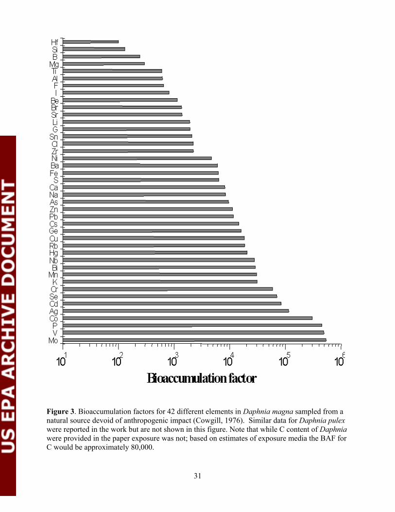
Figure 3. Bioaccumulation factors for 42 different elements in Daphnia magna sampled from a natural source devoid of anthropogenic impact (Cowgill, 1976). Similar data for Daphnia pulex were reported in the work but are not shown in this figure. Note that while C content of Daphnia were provided in the paper exposure was not; based on estimates of exposure media the BAF for C would be approximately 80,000.

31

Depending on the organism and the metal, BCFs can range from less than 1 to over 106 in aquatic organisms (IAEA, in press; McGeer et al., 2003). In many species, especially the smaller ones with high surface area to volume ratios, metals like Pb, Ru, Zr, certain lanthanides, and transuranic elements are normally concentrated more than physiologically important elements such as Zn, Cu, and Co. This occurs since many of these non-essential elements are extremely particle-reactive in water and are more apt to sorb to surfaces. For example, phytoplankton cells quickly take up metals and can reach extremely high bioconcentration factors (Table 1). These elevated BAF values are interesting from the point of view of metal uptake but this accumulation has not been linked to a potential for direct toxic impact to the accumulating organism. However, the potential for secondary impacts related to the trophic transfer from phytoplankton up the food chain is possible but has not been characterized and is not well understood at this time (see Section 4.2.7).

Amongst the plankton, smaller organisms generally attain higher concentration factors than larger species because of greater relative surface area for adsorption of the former (Fisher, 1985). For these small planktonic organisms, bioconcentration factors on the order of 104 to 105

are not uncommon for several metals. Such high enrichment factors alone make small species potentially important in affecting subsequent metal redistribution throughout the water column and acting as enriched sources of these metals for trophic transfer. It must be noted that BCFs for metals can be highly variable and are inversely correlated to exposure concentrations (McGeer et al., 2003 and as discussed above), making representative single value BCF for a metal meaningless. While elevated BCF/BAF values have been measured (e.g., Table 1) and while they may provide for a simplified measure of bioaccumulation, linkages between BCF/BAF measures and detrimental impacts are generally lacking, making their use in a regulatory context problematic.

In summary, the BAF/BCF model has been derived and validated, both experimentally and theoretically, but only for a limited number of lipophilic, nonionic synthetic organic substances that undergo minimal metabolism within the animal (Feijtel et al., 1997). The fundamental differences that exist between between the physical, chemical and toxicological properties of organic and inorganic metal substances would indicate that this model will not apply to the latter. In fact, the extension of lipid solubility and fugacity based models to inorganic metals substances has been questioned previously (McCarty and Mackay, 1993; Barron, 1990; Franke et al., 1994). Furthermore, as reviewed by Barron (1990), extrapolation of models to other substances beyond the database of tested organic substances has usually been discouraged. Also, a number of reviews have illustrated that the BAF/BCF (and Kow) model are inappropriate for assessing inorganic metal substances (Barron et al., 1990; Franke et al., 1994; Parametrix, 1995; Chapman, 1996; Chapman et al., 1996; Franke, 1996; McGeer et al., 2003). The approach of using one simplified bioaccumulation model (BCF and BAF) and applying it to inorganic metals ignores the basic physical and chemical differences between organic and inorganic substances and is not supported by theoretical and empirical weight of evidence. Based on the inherent assumptions of the BCF and BAF model and on the environmental and toxicological behavior of the organic substances from which they were developed and validated, for the vast majority of inorganic metals evaluated, the scientific basis for broad application of the BAF/BCF model is lacking in the context of hazard assessment. The regulatory implications and potential solutions are discussed in Section 5.1.

32

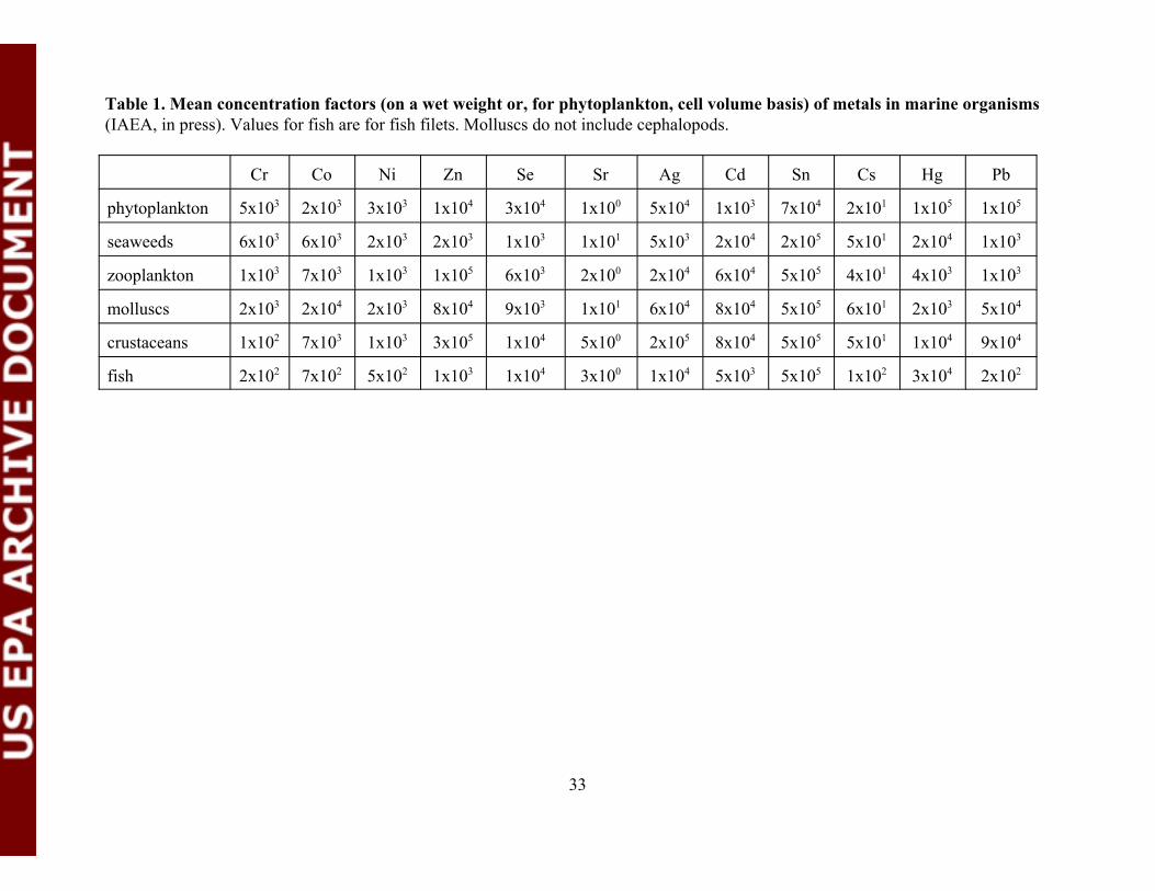
Table 1. Mean concentration factors (on a wet weight or, for phytoplankton, cell volume basis) of metals in marine organisms (IAEA, in press). Values for fish are for fish filets. Molluscs do not include cephalopods.

Cr Co Ni Zn Se Sr Ag Cd Sn Cs Hg Pb

phytoplankton 5x103 2x103 3x103 1x104 3x104 1x100 5x104 1x103 7x104 2x101 1x105 1x105

seaweeds 6x103 6x103 2x103 2x103 1x103 1x101 5x103 2x104 2x105 5x101 2x104 1x103

zooplankton 1x103 7x103 1x103 1x105 6x103 2x100 2x104 6x104 5x105 4x101 4x103 1x103

molluscs 2x103 2x104 2x103 8x104 9x103 1x101 6x104 8x104 5x105 6x101 2x103 5x104

crustaceans 1x102 7x103 1x103 3x105 1x104 5x100 2x105 8x104 5x105 5x101 1x104 9x104

fish 2x102 7x102 5x102 1x103 1x104 3x100 1x104 5x103 5x105 1x102 3x104 2x102

33

Metal Uptake in Marine Organisms: Aquatic animals can accumulate metals from both the dissolved phase directly and from ingested food. The relative importance of the different uptake pathways has received considerable attention in recent years, in part because contaminants, including metals, accumulated from food deposit in animal tissues, different from those obtained from the dissolved phase, and this may ultimately have consequences for subsequent trophic transfer and toxicity (Hook and Fisher, 2001; Fisher et al., 1996; Bjerregaard et al., 1985). Bioenergetic-based kinetic models used to describe the accumulation of contaminants in aquatic animals have been developed relatively recently and have been successfully applied to a variety of organic and inorganic contaminants. These models provide a broad framework for addressing controls on contaminant bioaccumulation for diverse organisms and can be used for studying contaminant bioavailability and determining the relative importance of different routes of contaminant accumulation, including that of metals (Wang et al., 1996; Landrum et al., 1992). The models are flexible enough to incorporate environmental variability in contaminant sources, contaminant concentrations, food availability, and organism growth rates in their predictions of organism contaminant levels.

One widely used version of these models treats contaminant accumulation as a first order function of contaminant concentrations in particles and water.

dC/dt = (ku * Cw) + (AE * IR * Cf) - (ke + g) * C (Eq. 4.1)

where C is the metal concentration in the animals (:g g-1), t is the time of exposure (d), ku is the uptake rate constant from the dissolved phase (L g-1 d-1), Cw is the metal concentration in the dissolved phase (:g L-1), AE is the assimilation efficiency of the metal from ingested particles (%), IR is the ingestion rate of particles (mg g-1 d-1), Cf is the metal concentration in ingested particles (:g mg-1), ke is the efflux rate constant (d-1), and g is the growth rate constant (d-1). At steady state, this equation simplifies to:

Css = (ku * Cw) + (AE * IR * Cf) (Eq. 4.2) (ke + g).

where Css is the steady-state concentration of metal in the organism (:g g-1). The efflux ew) and particle (kef) components (Eq. 4.3).parameter, ke, can be split into solute (k

Css = (ku * Cw) + (AE * IR * Cf) (Eq. 4.3) (kew + g) (kef + g)

Except for growth, all of the parameters in Eq. 4.2 are readily estimated from laboratory radiotracer studies. The importance of growth varies, depending on the species and stage of maturity.

Application of this kinetic model has shown that laboratory-based measurements of AE, ku, kew and kef are applicable to field situations for populations of marine mussels (Wang et al., 1996; Fisher et al., 1996), Ag, Cd, Co and Se in clams (Griscom et al., 2002; Luoma et al., 1992), Po in copepods (Stewart and Fisher, 2003; Fisher et al., 2000), Se in fish (Baines et al., 2002), and freshwater mussels (Roditi et al., 2000). Site-specific model predictions for metal concentrations in animal tissues are strikingly close to independent field measurements for

34

diverse water bodies, suggesting that it is possible to account for the major processes governing contaminant concentrations in aquatic animals and that the laboratory derived kinetic parameters are applicable to natural conditions. Generally, efflux rates in the studies cited here do not differ enormously among the various metals nor do kef and kew values differ greatly from each other for any given metal. However, efflux rates in higher animals like fish have been shown to vary more appreciably. Assimilation efficiencies of ingested metals also vary greatly among metals and even appreciably for any single metal with the food source and diverse environmental factors (Wang and Fisher, 1997). Uptake rate constants of metals from the dissolved phase (ku) also vary appreciably among metals (Wang and Fisher, 1997).

Because some of the parameters in Eq. 4.2 may not be available, certain modifications could enable useful computations. For example, the estimate of metal uptake from the dissolved phase can be described as:

Iw = " w * FR * Cw = ku * Cw (Eq. 4.2)

where Iw is the metal influx rate from the dissolved phase (:g g-1 d-1)—note that this parameter can be measured experimentally—and ku is the dissolved uptake rate constant (L g-1 d-1) of the metal, which equals absorption efficiency of dissolved metal across the gill (" w) times the filtration rate of the animal (FR). The ku can be computed from the relationship between Iw and Cw. When Cf is not known, it can be calculated from Cw by applying a Kd value for suspended particulate matter:

Cf = Cw * Kd (Eq. 4.5)

where Kd is the partition coefficient of a metal on the ingested particles (L kg-1).

The fraction of total contaminant uptake attributable to uptake from the dissolved phase and particulate ingestion can be calculated as:

Fw = Cw, ss / Css (Eq. 4.6) Ff = Cf, ss / Css (Eq. 4.7)

where Fw is the proportion of accumulated metal obtained from the dissolved phase, and Ff is the proportion of accumulated metal obtained from food.

Note that Cw (dissolved concentration, :g L-1) and Cf (particulate concentration, :g mg-1) are directly dependent on the total suspended solids load (TSS), Kd, and the total concentration (Ct, :g L-1) of metal in the water column (that is, dissolved plus particulate metal concentration).

Ct = Cw + (Cf * TSS) (Eq. 4.8) * Kd * TSS) (Eq. 4.9)Ct = Cw + (Cw

Thus, t (Eq. 4.10)Cw = [1 / (1 + TSS * Kd)] * C

35

It is noteworthy that there is no constant proportionality between Css and Ct; that is, bioconcentration factors vary with biological factors like physiological state and environmental factors like temperature. Changes in any of the kinetic parameters can significantly affect the ratio of Css to Ct, which is a mathematical expression of the widely employed bioaccumulation factor (BAF). The BAF as defined here thus considers both dissolved and particulate metal uptake in animals:

Css ku (AE * IR * Kd) 1 BAF = ____ = [ _______ + _____________ ] * [____________ ] (Eq. 4.11)

Ct (kew + g) (kef + g) (1 + TSS * Kd)

Because metals in most natural waters (particularly marine waters) are predominantly in the dissolved phase (defined here as passing through a 0.2 :m filter), even for the most particle-reactive metals (i.e., Cw ~ Ct), BAF values for metals tend not to differ appreciably from bioconcentration factors (which are equivalent to Css/Cw), except in waters with very high particle loads. However, Kd is highly variable for metals such as Cu, Zn, and Cd, even when evaluated using high quality datasets, suggesting caution since the application of Eq. 4.ll is not without substantial variability/uncertainty.

In addition to the organism specific and site specific factors that add complexity to modeling and its interpretation issues, certain methodological issues should be considered. For example, uptake kinetic studies often depend on radiotracer techniques which virtually eliminate some metals from typical study designs (e.g., Cu). As well, for chronic bioaccumulation, it may take organisms such as fish many months to reach steady state with their exposure conditions. For example, there is a wide diversity of tissue specific half-times to saturation in rainbow trout, from a few days for Cu to almost a year in the case of Cd accumulation in the kidney (McGeer et al., 2000c).

The Biotic Ligand Model. Modeling the interactions of metals with biological surfaces, particularly the fish gill, was advocated by Bergman and Dorward-King (1997) as a method of predicting the acute toxicity of metals in freshwater systems. These biotic ligand models (BLM) are based on the gill surface interaction model for trace metal toxicity proposed by Pagenkopf (1983). BLMs are among the more comprehensive of metal accumulation and toxicity models as they link metal bioaccumulation and bioavailability with toxic impacts (reviewed Paquin et al., 2002). The BLM approach predicts toxicity by considering the geochemical equilibrium within the exposure medium and the relationship with exposure conditions and the organism (the biotic ligand). The model combines factors influencing aquatic speciation (e.g., pH, temperature, organic and inorganic anionic complexation) as well as other abiotic factors, specifically cationic competition (e.g., Na+, K+, Ca2+, Mg2+). The combined effects of speciation and cationic competition in predicting metal toxicity have been successfully applied (Di Toro et al., 2001; Santore et al., 2001; McGeer et al., 2000c; de Schamphelaere et al., 2002; Heijerick et al., 2002). The success of BLM approach in predicting metal toxicity results, at least conceptually, from the fact that the model can distinguish metal that will bioaccumulate and cause toxicity from the total metal pools in an organism as well as the bioavailable metal pool in the exposure media.

The success of the BLM approach is based on studies such as those by MacRae et al., (1999) which demonstrated that Cu accumulation at the site of toxicity (the gill) was directly

36

correlated with toxicity. The modeling approach assumes that toxicity (i.e., LC50) is associated with a critical level of metal accumulation at/on the biotic ligand (Di Toro et al., 1999, 2001) and applies the characterization of gill metal interactions (Playle et al., 1993a,b; Janes and Playle, 1995). Therefore, even though metal concentration in the water that produces toxicity can vary, the amount of bioaccumulated metal at the site of toxicity (the fish gill) does not.

Because the complexation of metal to the biotic ligand is considered in conjunction with other ligands and competing cations in the water column, much of the variability in LC50 concentrations associated with differences in water chemistry can be explained by this methodology. Although the original development of BLM approaches were based a mechanistic understanding of metal uptake (Playle et al., 1993a, b) and the physiology of toxic responses (Morgan et al., 1997; McGeer et al., 1998), once the proof of principle had been demonstrated calibrating the BLM approaches directly to toxicity was possible. This allowed for the extension of modeling approaches to species such as algae (Heijerick et al., 2002) and daphnia (de Schamphelaere et al., 2002), which are toxicologically relevant but more difficult to characterize in terms of accumulation at the site of toxic action.

The BLM approach for predicting metal toxicity is continuing to be developed for the effects of Ag, Cd, Cu, Ni, Pb, and Zn. Most of these developments are focusing on acute impacts, but there is considerable interest in chronic toxicity (Paquin et al., 2002). The broadening of these mechanistic models presents a number of challenges. For example, geochemical speciation of metals relative to bioaccumulation and toxicity needs refinement, particularly for the role of natural dissolved organic matter, a key factor in moderating toxicity but whose activity is not well understood. In terms of chronic impacts, the physiological mechanisms associated with toxicity are not well characterized, so the modeling endpoint, accumulation of metal or dose delivered to the site of impact, is unclear. Acclimation responses can influence bioaccumulation at the site of toxicity, and incorporating these into chronic toxicity modeling will also present a challenge. As well, species can differ considerably with regard to the forms of metal taken up as well as their relative toxicities. In spite of these and other issues that add complexity, the BLM approach is mechanistically based—explicitly designed to consider metal biogeochemistry; therefore, it presents a viable avenue toward understanding and predicting the impacts of metals.

4.2.7 Metabolism/Detoxification

Even though the degree of uptake and assimilation of a metal is a key factor in bioaccumulation, physiological processes, renal, biliary, or branchial, generally control elimination, sequestration, detoxification, and storage occurs (Mason and Jenkins, 1995; McDonald and Wood, 1993). These physiological processes often actively regulate metal bioaccumulation via dynamic feedback systems that respond to environmental loading and maintain homeostasis (Hamilton and Mehrle, 1986; Chapman et al., 1996; Wood, 2001). The ability to control, detoxify, store, and/or eliminate is due to nutritional dependency (for essential metals) and to the fact that biota have evolved in the presence of metals. Many aquatic animals have the ability to sequester and store metals in detoxified forms, such as in inorganic granules, or bind to metallothionein-like proteins (see previous discussion). The use of granules as a storage mechanism is of particular note in the context of BCFs, because extremely high body burdens are often associated with this storage mechanism but unrelated to adverse impact. It is

37

possible, however, that a detoxified metal may have the potential to become bioavailable to consumer (predator) organisms and cause deleterious impacts, and this is worthy of study and quantification. Experimental approaches designed to assess this potential for trophic transfer should endeavor to characterize real food web linkages and to distinguish between the bioavailability of detoxified forms and other bioaccumulated forms of metal. It is interesting to note that the potential for trophic transfer of bioaccumulated metal is not captured through the application of BCF and BAF data as criteria thresholds, as is done in hazard assessment.

Zn is an example of an essential element for which metabolic regulation of internal concentrations has been demonstrated. At low environmental Zn levels, animals are able to sequester and retain Zn in tissues for essential functions (Vallee and Falchuk, 1993). When Zn exposure levels are chronically elevated, aquatic animals are able to control bioaccumulation. There is clear evidence that many species actively regulate their body Zn concentrations including: Crustacea such as Homarus gammarus, Carcinus maenas, Maia squinado, Crangon crangon, Palaemon elegans, P. serratus (Rainbow and White, 1989), and Austropotamobius pallipes (Devineau and Triquet, 1985; Rainbow and Dallinger, 1993); the oligochaetes Lumbriculus variegatus and Nereis diversicolor (Rainbow and Dallinger, 1993); mussels such as Mytilus edulis, Dreissena polymorpha, Unio pictorum, and Velesunio ambiguus (Rainbow and Dallinger, 1993; George and Pirie, 1980; Kraak et al., 1993); the gastropod Nucella reticulatus (Kaland et al., 1993); and Oncorhynchus mykiss (Alsop et al., 1999a; Bradley et al., 1985).

As it does with Cu, the amphipod Echinogammarus pirloti does not actively excrete excess Zn, but takes it up at a low net rate relative to its body growth rate (Rainbow and White, 1989), thus illustrating another burden control strategy. Detoxification both through binding to proteins (Rainbow et al., 1980) as well as storage as Zn phosphate granules (Rainbow and White, 1989; George et al., 1978; Rainbow et al., 1990) has also been discussed. While the chironomids Chironomus riparius and Stictochironomus histrio do not appear to actively regulate their zinc body burdens, Zn is lost with each cast exuvium (Timmermans and Walker, 1989).

Although total Zn burden is not well correlated with Zn exposure, radiotracer studies in rainbow trout have shown that chronic waterborne Zn2+ exposure results in dramatic and complex alterations in gill uptake kinetics (Alsop and Wood, 2000) and that these are linked to Ca2+ dynamics (Hogstrand et al., 1995). Included in the changes are a decreased affinity and an increase in the total number of binding sites (Alsop and Wood, 2000). Therefore, altering gill uptake dynamics is an additional metabolic response that controls Zn bioaccumulation and is part of the acclimation response.

It is generally agreed that the bioaccumulation of Cd does not serve a nutritional purpose and there is little evidence of active regulation of internal Cd concentrations. However, there is good evidence that some level of physiological control over bioaccumulation exists. For example, reduced branchial uptake in response to exposure has been demonstrated in rainbow trout (Hollis et al., 1999, 2000; Szebedinsky et al., 2001). As well, growth dilution of Cd stores in decapods shows that a form of regulation is possible (Rainbow et al., 1990). Detoxification of accumulated Cd is also common. For example, binding of Cd to low molecular weight proteins such as metallothionein occurs in many animals (Mason and Jenkins, 1995), including rainbow trout (Hollis et al., 2000); the barnacle Semibalanus balanoides (Rainbow et al., 1990); the scallop Mizuhopecten yessoensis (Lukyanova et al., 1993); the marine gastropod Nassarius

38

reticulatus (Kaland et al., 1993); and possibly Daphnia magna (Bodar et al., 1990). An example of an animal with tissue-specific granule storage of Cd is the marine isopod Idotea baltica where granules are stored in the hepatopancreas (de Nicola et al., 1993). These studies illustrate that Cd burdens significantly above “normal” levels can be tolerated and physiological processes adapted to result in acclimation.

Similar to Cd, there is no nutritional role for Pb; however, detoxification and storage have been documented for this metal. Pb will bind to metallothionein and probably has a higher affinity for other metabolic ligands, as it is often associated with deposited inorganic granules with high concentrations of calcium (Rainbow, 1988). Hopkin and Nott (1979) demonstrated that the shore crab (Carcinus maenas) detoxifies lead in calciferous granules in the midgut gland. The detoxification and storage of Pb in shellfish has been suggested for the zebra mussel Dreissena polymorpha (Kraak et al., 1994; Bleeker et al., 1992), the blue mussel Mytilus edulis (Talbot et al., 1976; Schulz-Baldes, 1974), the Eastern oyster Crassostrea virginica (Shuster and Pringle, 1969; Pringle et al., 1968; Zaroogian et al., 1979), and the soft-shell clam Mya arenaria (Pringle et al., 1968).

Studies with Cu clearly demonstrate that aquatic animals are able to control Cu bioaccumulation, as would be expected for this essential element. A wide variety of aquatic animals are able to regulate internal Cu concentrations including Palaemon elegans, Crangon crangon, Homarus gammarus, Carcinus maenas and Echinogammarus pirloti reviewed by Rainbow and White (1989) as well as Neanthes arenaceodentata (Pesch and Morgan, 1978) and Eudistylia vancouveri (Young et al., 1979). Additionally, it has been shown that fish such as rainbow trout actively regulate Cu via sequestration into the liver and elimination via the bile, a process that involves Cu-specific transport mechanisms (Grosell et al., 1997, 1998, 2001). This control of bioaccumulation also extends to an ability to adjust uptake based on exposure concentrations (Kamunde et al., 2002). Detoxification of Cu through binding to metallothioneinlike proteins has also been shown to be of significance (Rainbow et al., 1980; Mason and Jenkins, 1995; McDonald and Wood, 1993; Rainbow et al., 1990). In addition, detoxification and storage of Cu in granules has been shown (Rainbow et al., 1990; Brown, 1982).

4.2.8 Biomonitoring as a Tool for Bioaccumulation

Because metals can speciate in many ways in water, and because not all of these chemical species are available for biological uptake (Campbell, 1995), evaluating the so-called “bioavailable” fraction can be important. Biomonitoring programs have been established for this purpose, with particular emphasis on using bivalve molluscs such as mussels. Using marine mussels to serve as sentinels of coastal contamination was proposed and first tested in the 1970s (Goldberg et al., 1983, 1976). It has since been widely accepted throughout the world and is currently in practice in different sized national programs in many regions.

Numerous reviews have identified the factors that make mussels useful as bioindicators of coastal contamination (e.g., Phillips, 1980). The following attributes are: among the most attractive: mussels are ubiquitous, sessile, easy to collect, not easily poisoned by high contaminant concentrations, and any contaminant within the tissues of the animal is, by definition, a contaminant that is in a form that was available for bioaccumulation (“bioavailable”). Clearly, knowing the bioavailable fraction is critical, since the principal

39

concern regarding contaminants is tied to the potential effects on living organisms (including man). But only bioaccumulated contaminants have the potential to impact living organisms. The uptake of contaminants in mussels gives us an idea of the concentration of bioavailable contaminants in a region. Moreover, contaminants in mussel tissues, including shells, have been shown to reflect ambient dissolved contaminant concentrations (Wang et al., 1996; Bjerregaard et al., 1985), and the mussel serves to integrate its past contaminant exposure over time.

Thus, analyzing mussels does not just provide an instant “snapshot” of the immediate conditions but rather a picture of contaminant levels over a period of weeks to months. Because contaminant concentrations in mussel tissues seem to generally reflect ambient contaminant concentrations, the underlying assumption that these organisms actually reflect environmental concentrations appears to be valid. For many marine organisms, the uptake of metals from water is proportional to ambient metal concentrations, although concentrations of several essential elements (e.g., Zn, Fe, Mn) may be physiologically regulated so that internal concentrations in certain species would show little variation in response to changing levels in their surroundings.

Because biological factors can greatly influence the extent to which metals concentrate in mussel tissues, existing monitoring programs make sure that these are considered in their sampling protocols (NOAA, 1998). For example, mussels that are spawning can mobilize certain metals more than others, and a misleading picture of the bioavailable concentrations of those metals can result if spawning mussels are sampled (Dahlgaard, 1986).

4.3 Terrestrial

Current issues and dictums of terrestrial bioavailability and bioaccumulation include:

• Empirical field and/or lab data with sufficient quality of design and conduct are much superior to the estimates of metal bioavailability obtained from less certain modeling.

• A “triad” of three factors: exposure + metal type + receptor are legs that determine the environmental bioavailability of a metal (like a tripod that will topple without all three legs).

- Exposure: Oral route of incidental soil ingestion of metals predominates for terrestrial vertebrates; dermal and inhalation routes are inconsequential.

- Metal type: Metals can not be easily lumped together, since their salts or forms vary substantially (e.g., PbS versus PbCO3, or Hg° versus HgCl or CH3Hg).

- Receptor: The intended target for risk assessment should be specified, or the most vulnerable/sensitive receptor should be measured and assessed for the protection of all other subpopulations, as small changes in physiology and pathology can produce substantial changes in bioavailability results.

• “Dynamic” target: Bioavailability studies must specify exactly and should test the ranges of conditions of exposures, metals, and receptor characteristics to accurately measure the anticipated ranges of metal bioavailability, since minor experimental changes can produce major changes in bioavailability estimates.

• “Exposure unit” for human health or “area use factor” specification: The area and time of exposure to a metal for the receptor of interest must be known, because spatial and temporal

40

averaging of soil sampling is needed (e.g., home range or feeding range areas for mobile wildlife during the times of the year when receptors are exposed to metals at a site).

Integrated multimedia biokinetic models are more predictive than simple models:

• “Validate, calibrate, verify, & bind” every model: As experts have noted, “All models are wrong, but some are useful”and “The best model of man is man”(i.e., avoid apples versus orange comparisons). Anything can be modeled, but not everything should be modeled, nor can most things be modeled with sufficient amounts of accuracy and reliability. A good model must always be validated (via PARCC—precision, accuracy, representativeness, comparability, and completeness—and other criteria) for its predictive value, calibrated in the lab, and then verified for the specific study. It should not only provide outputs as best estimate point values, but also confidence limits around those outputs (e.g., +/- 250%).

• “Variable” target: Strong, predictive models must specify all assumptions and set the bounds of exposure and toxicity to establish the amount of protectiveness (more-so than predictiveness) from excess risk that could be affected by adjustments to bioavailability default factors; biota toxicity endpoints may be used as surrogates of indirect estimates of bioavailability under controlled laboratory studies, but the many uncontrollable confounding factors in field conditions make such tests highly variable and unreliable for use in risk assessment.

• “In vitro solubility” models: Good tool to aim for developing as a screen, but few examples exist that are validated through calibration with an acceptable in vivo bioavailability study (since small deviations can make tremendous differences in solubility results of metals in these tests); most solubility tests that have not been thoroughly calibrated with a validated in vivo model will fail to predict bioavailability and bioaccumulation, but, at best, might only provide estimates of relative dissolution rates of various metal salts.

• “Tissue:soil ratio” models: These often are too simplified to work with any confidence or reliability in estimating adjustments to bioavailability of metals, due to the dynamic nature and many confounding factors involved—some metals are regulated and remain at fairly constant concentrations over varying soil concentrations (may have flat or even U-shaped dose-response curves), or metal uptake may change dramatically with plant or animal physiology (senescence of plants, or translocation of metals during emaciation or pregnancy) or with wildlife behavior leading to changes in feeding patterns.

Standardization of metrics (e.g., bioaccumulation factor) for bioavailability adjustments in risk assessment is needed, which should be specified in general by EPA or modified for specific sites per data quality objectives (DQOs):

• Which (soil metal) should be measured as the denominator? For example, sieved versus total or both (to determine amount of enrichment and to use for remedial purposes), gradients, valid references, co-located (biota) soil samples, mixed or averaged, vertical depths, composites, seasonal deposition, geophysical measures (predominant salt types, particle sizes, sources, occluded surface), etc.

41

• Which (tissue metal) should be measured as the numerator? For example, toxicity based, whole body, specific tissue, slope from multiple doses/concentrations versus ratios from limited samples (of metals in tissue versus soil), washed versus unwashed plants, seasonal differences in uptake (e.g., early growth versus senescence), etc.

• Which animal model and approach for in vivo and in vitro studies of bioavailability should be adopted by EPA as a template for other metals?

- Human: EPA Region 8’s lead and arsenic studies? Others? Why? Why not? - Wildlife: Co-located exposure-unit food chain studies? Others? Why? Why not? - Plants: Co-located root-tip soil washed-plant seasonal tissue studies? Others? Why?

Why not?

4.3.1 Human

Absolute versus Relative Bioavailability. The recent NRC report (NAS, 2002), on Bioavailability of Contaminants in Soils and Sediments, contains an exhaustive amount of review material on the historical and conceptual development of studies on the bioavailability of metals in soils (beginning on page 27, NAS, 2002). Some of the more important conceptual definitions and distinctions are paraphrased:

When bioavailability is considered as the fraction of the chemical that is absorbed into systemic circulation, two operational definitions are important—absolute and relative bioavailability. The amount of chemical that is ingested lies on the surface of the skin or is inhaled is called the applied dose. The amount that is absorbed and reaches the systemic circulation is called the internal dose; it is dependent upon the absolute bioavailability of the chemical, i.e., the fraction of the applied dose that is absorbed. Clearly, absolute bioavailability can never be greater than 100 percent.

Relative bioavailability represents a comparison of absorption under two different sets of conditions. Examples might include absorption of a chemical from two different routes of exposure, or from the same route of exposure but from two different types of environmental samples. Relative bioavailability says nothing directly about the amount of chemical absorbed into the body; it only describes the relationship between the amount absorbed under two different circumstances. For example, if a chemical is absorbed equally as well through the skin as from the gut, the relative bioavailability (dermal versus ingestion) for these exposure routes is 100 percent, even though the fraction absorbed (absolute bioavailability) from each of the routes may be only 5 percent. Relative bioavailability can be greater than or less than 100 percent.

Incidental Soil Ingestion and RAF. By default for risk assessment, the relative absorption factor (RAF) that is used for intake calculations is set at 1.0 for contaminants, including metals, unless convincing data can show that this value should be changed for the risk and exposure scenario under evaluation. As described in the NRC Report (NAS, 2002), the intake equation for incidental ingestion of soils is shown below. Because the oral route and incidental soil ingestion of metals is the risk driver for most environmental scenarios, the RAF endpoint is the most effective and practical target for relative bioavailability (RBA) studies. The tissue for measurement of the absorbed metal in soil should depend upon tissue measured in the key toxicity study used as the risk-based benchmark.

42

On occasion, epidemiological (Griffin et al., 1993; Calabrese et al., 1987) or human subject studies (Maddaloni and Graziano, 1998) can be used to help estimate the ingestion of soil and bioavailability of metals such as arsenic via urine samples and lead via blood samples with stable isotope dilution. If designed and conducted properly, their value for risk assessment may be of more than that of other bioavailability studies for adjustments to exposures, as an estimate of absolute bioavailability is provided rather than RBA.

An important consideration in such studies is to accurately define the “exposure unit,” which involves the proper averaging area for the C (concentration) term and the correct temporal terms. For example, for EPA’s integrated exposure uptake biokinetic (IEUBK) lead model, the C term is the average surface (usually 0 to 2 inches) concentration in a child’s residential yard, and the time of exposure is the chronic average daily intake from 0-6 years of age during the period of neurotoxic vulnerability. Other metals may have different spatial averaging areas (and depths) and averaging times, depending on the exposure scenario and “completed” pathways of major contributions of exposure. As an example, cancer endpoints may have chronic exposures averaged over adult lifetimes, while non-cancer endpoints may have sub-chronic exposures averaged for shorter durations of exposures related to shorter toxicologic onsets.

Human Health Bioassays to Measure Bioavailability. As described in the recent NRC Report (NAS, 2002, p. 226), a variety of techniques are available to attempt to measure bioavailability. The approaches include biomarkers of exposure (e.g., ALA activity from lead exposure), cell culture studies, isolated gastrointestinal tract tissue, whole animal approaches, and clinical studies. Of these options, the use of whole animals is most feasible (Weis and Lavelle, 1991), while clinical studies offer desirable advantages but present many obstacles (Maddaloni et al, 1998).

Blood Measures. As generally described in the NRC Report (NAS, 2002, pp. 231-233), the area under the concentration versus time curve (AUC) is most often measured for gastrointestinal absorption. Blood or plasma concentrations are plotted against time, and the area under the concentration versus time profile (AUC) is calculated. In order to determine absolute oral bioavailability, the AUC following oral administration (AUCoral) is compared with the AUC after intravenous administration (AUCiv), the latter representing the AUC expected if the entire oral dose reaches the systemic circulation. The equation below represents the calculation of absolute bioavailability (Fabsolute) based on a single oral dose:

AUCoral x DivBlood-derived Oral ABA = Fabsolute = AUCivxDoral

An analogous approach can be used to assess relative bioavailability (RBA), by measuring the relative absorption fraction (RAF). In this case, bioavailability under differing sets of conditions (e.g., oral bioavailability of a chemical from a soil matrix versus from water) can be obtained from the ratio of the their AUCs, with one condition designated as the reference for comparison (“condition A” in the equation below).

AUC(condition B) x Dcondition A Blood-derived Oral RBA = RAF = Frelative =

AUC (condition A) x D condition B

As with the measurement of absolute bioavailability, doses of different sizes can be used,

43

but only if they are in the linear (i.e., non-saturable) pharmacokinetic range. In addition to providing information on the extent of absorption of chemical, blood, or plasma, data provide the best information on the rate of absorption. Although the method can theoretically be applied to virtually any chemical, this approach is best suited for chemicals eliminated from blood in a matter of hours to a few days. Also, reliable AUC measurements require several blood or plasma samples with chemical concentrations that are measurable. Animal subjects must be large enough to provide the number of samples and blood volume dictated by the experimental design and the sensitivity of available analytical methods. This limits the utility of small animals for these studies and often makes testing of environmentally relevant doses of chemicals difficult.

Urine Measures. Many chemicals are excreted extensively in urine following their absorption, and analysis of the urine can provide an indication of absorbed dose. Typically, the animal subject is given a measured dose of the chemical, and urine is collected over time. The appropriate urine collection period depends on the elimination rate of the chemical but is usually extended until the chemical reaches undetectable or background concentration in urine. Based on the concentration of chemical in urine samples and their volumes, the cumulative amount excreted is calculated.

The absolute oral bioavailability (ABA) of a chemical can be calculated from the amount excreted following an oral dose (Aurine-oral) divided by the amount excreted after an intravenous dose (Aurine-iv). The intravenous dose is intended to represent the amount excreted in urine if the entire oral dose is absorbed. If doses of different sizes are used, the excreted amounts can be corrected for each dose, if it is known or can be assumed that the amounts excreted are linearly related to dose.

Aurine−oral xDivUrine-derived Oral ABA = Fabsolute = Aurine−iv xDoral

Sometimes, urinary excretion data are used to draw inferences on absolute bioavailability without benefit of a comparison with an intravenous dose. The amount excreted in urine provides an indication of absorbed dose only if other routes of excretion (e.g., biliary, pulmonary) are negligible, and elimination of the dose of chemical is complete. Because these conditions are rarely satisfied fully, bioavailability is usually underestimated by this method. Urinary excretion data can also be used to assess relative bioavailability (RBA) by comparing the excreted amount under two different dosing conditions.

Aurine( condition B) x Dcondition A Urine-derived Oral RBA = RAF = Frelative =

Aurine(condition A) x D condition B

Fecal measures. Fecal excretion represents the inverse of oral bioavailability. A metal that is not absorbed following oral exposure will ultimately be excreted in feces. Therefore, measurement of fecal concentration can be used as an indication of the extent of absorption. Measurement of oral bioavailability involves collection of feces following single or multiple doses of the chemical. The collection interval must be sufficiently long to accommodate the gastrointestinal transit of the dose. Also, some chemicals do not reach the systemic circulation, but are instead excreted in the feces as the epithelial lining is sloughed into the lumen of the gastrointestinal tract.

44

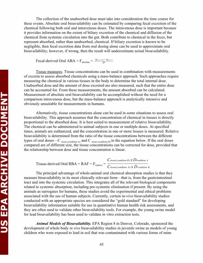
The collection of the unabsorbed dose must take into consideration the time course for these events. Absolute oral bioavailability can be estimated by comparing fecal excretion of the chemical following both oral and intravenous doses. The intravenous dose is important because it provides information on the extent of biliary excretion of the chemical and diffusion of the chemical from systemic circulation into the gut. Both contribute to chemical in the feces, but represent absorbed, rather than unabsorbed, chemical. If biliary excretion is known to be negligible, then fecal excretion data from oral dosing alone can be used to approximate oral bioavailability; however, if wrong, then the result will underestimate actual bioavailability.

Fecal-derived Oral ABA = Fabsolute = Afeces−oral

D − Afeces−iv

Tissue measures. Tissue concentrations can be used in combination with measurements of excreta to assess absorbed chemicals using a mass-balance approach. Such approaches require measuring the chemical in various tissues in the body to determine the total internal dose. Unabsorbed dose and the amount of dose excreted are also measured, such that the entire dose can be accounted for. From these measurements, the amount absorbed can be calculated. Measurement of absolute oral bioavailability can be accomplished without the need for a comparison intravenous dose, but the mass-balance approach is analytically intensive and obviously unsuitable for measurements in humans.

Alternatively, tissue concentrations alone can be used in some situations to assess oral bioavailability. This approach assumes that the concentration of chemical in tissues is directly proportional to the absorbed dose. It is best suited to measurement of relative bioavailability. The chemical can be administered to animal subjects in one or multiple doses. At specified times, animals are euthanized, and the concentration in one or more tissues is measured. Relative bioavailability is determined from the ratio of the tissue concentrations between the different types of oral doses—C tissue (condition A) and C tissue (condition B) in the equation below. If the oral doses compared are of different size, the tissue concentrations can be corrected for dose, provided that the relationship between dose and tissue concentration is linear.

Ctissue(condition B) x Dcondition A Tissue-derived Oral RBA = RAF = Frelative =

Ctissue(condition A) x D condition B

The principal advantage of whole-animal oral chemical absorption studies is that they measure bioavailability in its most clinically relevant form—that is, from the gastrointestinal tract and into the systemic circulation. This integrates all of the relevant biological components related to systemic absorption, including pre-systemic elimination if present. By using the animals as surrogates for humans, these studies avoid the experimental and ethical problems associated with the use of human subjects. Currently, certain in-vivo bioavailability studies conducted with an appropriate species are considered the “gold standard” for developing bioavailability information suitable for use in quantitative human health risk assessments, and they are often used to validate other bioavailability tools. For example, the young swine model for lead bioavailability has been used to validate in vitro extraction tests.

Animal Models of Bioavailability. EPA Region 8 in Denver, Colorado, sponsored the development of whole body in vivo bioavailability studies in juvenile swine as models of young children who were exposed to lead in soil that was contaminated with various forms of mine

45

wastes (Lavelle et al., 1991; Weis et al., 1992, 1993). At this time, no guidance or policy nor scientific precedence existed (other than that used for bioavailability by the pharmaceutical industry) for determining the relative bioavailability of metals in mine wastes. On one hand, it was argued that lead and arsenic from such mine sources was so insoluble and inert as to be unavailable and non-toxic to humans and other exposed receptors. U.S. EPA default exposure factors and early risk guidance documents required the use of the assumption of 100 percent relative bioavailability for any form of contaminant unless solid scientific data could prove otherwise. Early screening studies were devised to test the hypothesis that metals from mine wastes in soil were not bioavailable to a mammalian test subject, and this hypothesis was not supported (Lavelle, 1991; Weis, 1993); i.e., substantial mass of lead and arsenic in contaminated soil was absorbed from oral doses in a juvenile swine model.

As a result of this qualitative investigation, a program was initiated to develop a swine model of children for possible use in more quantitative analysis of lead bioavailability from mine wastes in soil. This Phase I characterization involved a set of soil-dosing studies that were undertaken through contracts with Weston and Michigan State University and included numerous outside parties from industry and academia for peer review of the process, study designs, and results. Blood-lead (PbB) AUC and tissue-lead concentration were measured as endpoints, with steady-state PbB and linearity of dose-related uptake of lead in tissues achieved within 14 days. Upon successful completion of these studies (Weis, 1994, 1995; Poppenga, 1994), the testing of 20 different lead-containing matrices (including 17 soils with mine wastes that included arsenic and other metals) was begun under Phase II studies. The results of these studies were quantitative and showed that lead from mine wastes in soil ranged significantly from under 10 percent to over 90 percent RBA when compared to PbAc control bioavailability (see Figure 4) (Henningsen, 1998). The results of these studies were subjected to outside peer review and found to be valid and acceptable for use in adjusting the RBA for lead in risk assessments, including the use of a calibrated in vitro solubility assay. However, preliminary studies of the same soil samples on arsenic RBAs (based on urine recoveries) were deemed to be premature due to lack of recoveries to account for mass balances of total arsenic doses (TERA, 1998).

The development of juvenile swine models to study the RBA of lead in soil as a model for children represents some of the more comprehensive and stronger science- and risk-based approaches for bioavailability. However, this model was specifically designed for quantitatively distinguishing RBA of lead in soil for children, and any other applications would need to have the model revalidated to ensure its predictiveness.

For example, during exploratory and model characterization studies, it was determined that testing the age/weight of the animal outside the defined “juvenile window” of post-weaning sizes of 7 kg to about 35 kg would decrease the RBA by about four-fold for the same doses of the identical materials. Likewise, testing the same doses in a pregnant animal would result in a RBA twice that of its identical non-pregnant counterpart. Conversely, studies performed to test the effect of adding clean soil volume to the sample had no appreciable effect on the RBA. However, some matrix effect may have been apparent with similar lead salts that had dissimilar RBAs. Attempts were made to try to mimic as closely as possible the typical exposure conditions experienced by the receptor population of concern; i.e., young children with mouthing

46

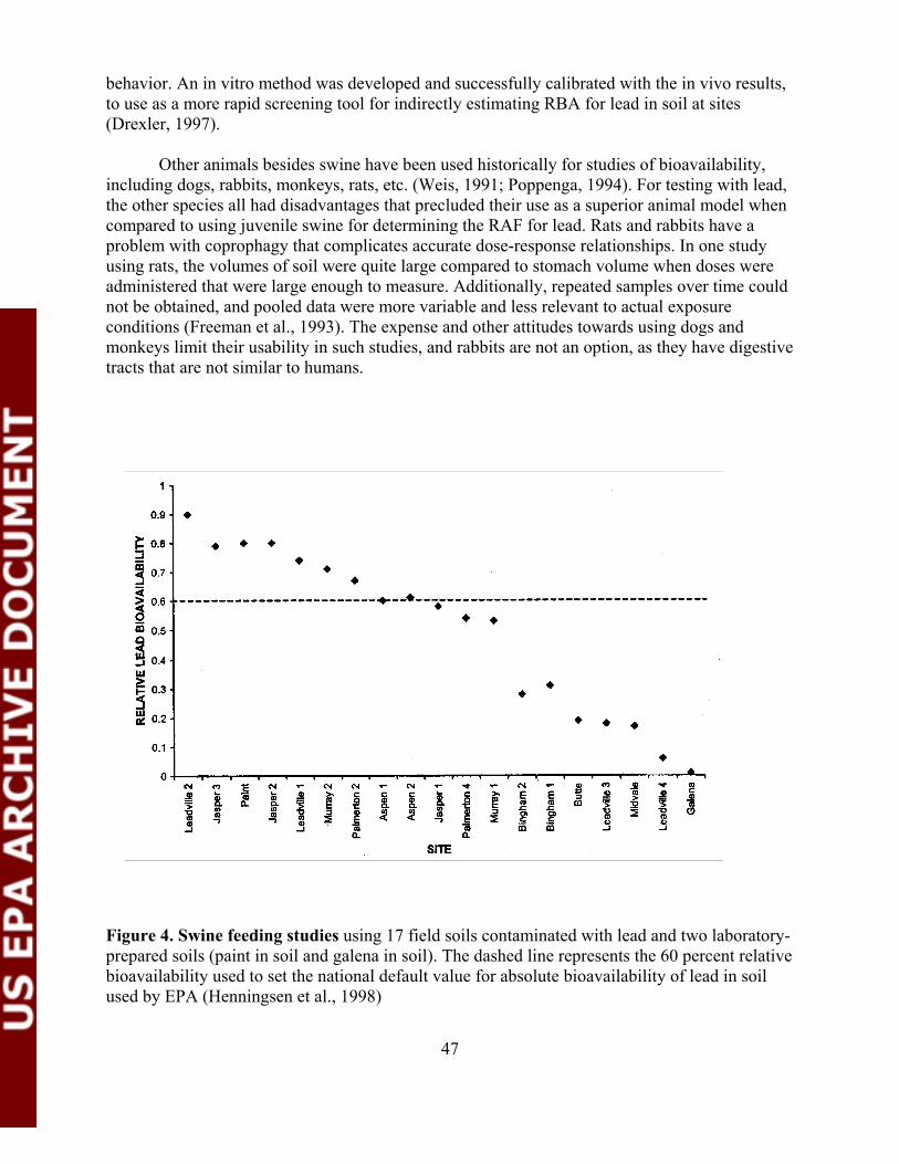
behavior. An in vitro method was developed and successfully calibrated with the in vivo results, to use as a more rapid screening tool for indirectly estimating RBA for lead in soil at sites (Drexler, 1997).

Other animals besides swine have been used historically for studies of bioavailability, including dogs, rabbits, monkeys, rats, etc. (Weis, 1991; Poppenga, 1994). For testing with lead, the other species all had disadvantages that precluded their use as a superior animal model when compared to using juvenile swine for determining the RAF for lead. Rats and rabbits have a problem with coprophagy that complicates accurate dose-response relationships. In one study using rats, the volumes of soil were quite large compared to stomach volume when doses were administered that were large enough to measure. Additionally, repeated samples over time could not be obtained, and pooled data were more variable and less relevant to actual exposure conditions (Freeman et al., 1993). The expense and other attitudes towards using dogs and monkeys limit their usability in such studies, and rabbits are not an option, as they have digestive tracts that are not similar to humans.

Figure 4. Swine feeding studies using 17 field soils contaminated with lead and two laboratory-prepared soils (paint in soil and galena in soil). The dashed line represents the 60 percent relative bioavailability used to set the national default value for absolute bioavailability of lead in soil used by EPA (Henningsen et al., 1998)

47

For arsenic studies, the rat is absolutely disqualified because it has a high-affinity red blood cell binding that makes its toxicokinetics unique among mammals, so that extrapolations of data are impossible. Mercury is another metal where different species have red blood cells with varying half-lives of mercury residence, which needs to be considered for bioavailability studies. Non-human primates have been used to estimate bioavailability of arsenic in soil at mining sites with some success, using the same animals repeatedly after clearing the arsenic which has a relatively short half-life in the body (Freeman et al., 1993). Recent studies with the EPA Region 8 soils in juvenile swine found that the mass-balance of inorganic arsenic in soil samples could be accounted for if the urine samples were further analyzed for organic arsenic, which the swine had metabolized and which the routine inorganic arsenic analytical methods had missed in the urine samples. Thus, the juvenile swine model may work suitably for arsenic RBA.

Additional considerations for designing good animal model studies of RBA include an appreciation for the role that homeostasis plays in metal regulation. Dietary minerals and other nutrients or metal cations and anions may either enhance or inhibit the absorption or distribution and elimination of other metals. As examples, vitamin D enhances Ca absorption, vitamin E enhances Se activity, Cu activity is affected by Mo and SO4 and its absorption may be affected by iron. When designing bioavailability studies, it is crucial to consider all sources (mainly dietary) of the metal under investigation for relative contributions to doses. For example, in the EPA Region 8 pig studies, normal corn based diets contained an equivalent amount of lead equal to the middle dose intended for the RBA studies, so a low-lead diet had to be created that was balanced and met minimal NRC nutritional needs for swine. Even so, the low-lead diet still contributed about 25 to 33 percent of the lead to the lowest dose tested.

Such problems with ambient metal concentrations may also be observed with arsenic and mercury, as well as with essential nutrients such as Cu, Se, Zn, Fe, and Mn. The hormonal state of the test subjects may also confound the RBA of metals, since many essential metals are regulated by hormonal mechanisms, or related non-essential metals may be affected by such physiological variations in test subjects. An example is the mobilization of calcium during gestation or lactation, and the corresponding changes in the RBA of lead during these times when compared to the same test animals that are not pregnant nor lactating. Certain diseases can cause changes in toxicokinetics or toxicodynamics that could affect the RBA results, such as with the loss of plasma proteins that bind and transport certain metals during certain renal pathology.

Perhaps the most developed mathematical model is EPA’s IEUBK model of blood lead in children (U.S. EPA, 1999a). This model was actually built from early engineering equations, had a biokinetic algorithm inserted, and was adapted to allow certain site-specific inputs (within certain set bounds). The output is a curvilinear graph of the probability of a child having a blood lead (PbB) concentration greater than a certain level (e.g., under the input conditions, the chance that an exposed child would have a PbB >10 ug/dl). EPA’s risk goal is to keep such probabilities of risk <5 percent for a PbB to exceed 10 ug/dl in a young child. The model has recently been adapted for use with MS Windows software and has been tested with a probabilistic input module (U.S. EPA, 2001a). EPA’s Office of Research and Development (ORD) is also testing an “All Ages Model” that is hoped to eventually model all ages and all risks from metals, according to the investigators. Examples of some RBA adjustments to metals for human health risk assessments are shown in the Table 2.

48

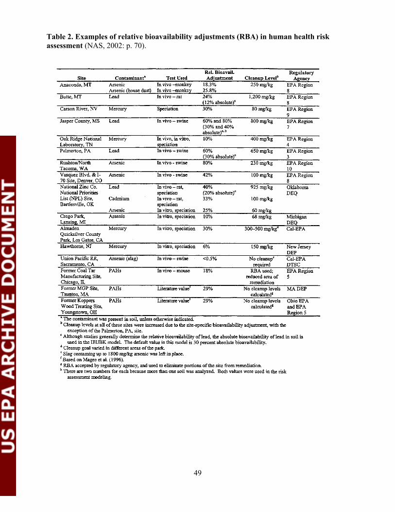
Table 2. Examples of relative bioavailability adjustments (RBA) in human health risk assessment (NAS, 2002: p. 70).

49

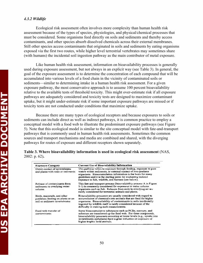
4.3.2 Wildlife

Ecological risk assessment often involves more complexity than human health risk assessment because of the types of species, physiologies, and physical/chemical processes that must be considered. Some organisms feed directly on soils and sediments and thereby access contaminants, and other species absorb dissolved chemicals across their external membranes. Still other species access contaminants that originated in soils and sediments by eating organisms exposed via the first two routes, while higher level terrestrial vertebrates may sometimes share (with humans) the incidental soil ingestion pathway as the main contributor of metal exposure.

Like human health risk assessment, information on bioavailability processes is generally used during exposure assessment, but not always in an explicit way (see Table 3). In general, the goal of the exposure assessment is to determine the concentration of each compound that will be accumulated into various levels of a food chain in the vicinity of contaminated soils or sediments—similar to determining intake in a human health risk assessment. For a given exposure pathway, the most conservative approach is to assume 100 percent bioavailability relative to the available tests of threshold toxicity. This might over-estimate risk if all exposure pathways are adequately considered and toxicity tests are designed to maximize contaminant uptake, but it might under-estimate risk if some important exposure pathways are missed or if toxicity tests are not conducted under conditions that maximize uptake.

Because there are many types of ecological receptors and because exposures to soils or sediments can include direct as well as indirect pathways, it is common practice to employ a conceptual model with a food web to illustrate the predominant exposure pathways (see Figure 5). Note that this ecological model is similar to the site conceptual model with fate-and-transport pathways that is commonly used in human health risk assessments. Sometimes the common sources and transport mechanisms and media are combined and shared, with the diverging pathways for routes of exposure and different receptors shown separately.

Table 3. Where bioavailability information is used in ecological risk assessment (NAS, 2002: p. 62).

50

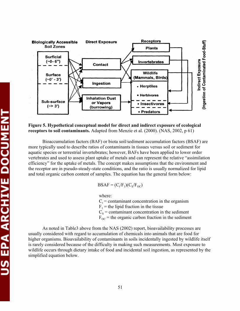
Figure 5. Hypothetical conceptual model for direct and indirect exposure of ecological receptors to soil contaminants. Adapted from Menzie et al. (2000). (NAS, 2002, p 61)

Bioaccumulation factors (BAF) or biota soil/sediment accumulation factors (BSAF) are more typically used to describe ratios of contaminants in tissues versus soil or sediment for aquatic species or terrestrial invertebrates; however, BAFs have been applied to lower order vertebrates and used to assess plant uptake of metals and can represent the relative “assimilation efficiency” for the uptake of metals. The concept makes assumptions that the environment and the receptor are in pseudo-steady-state conditions, and the ratio is usually normalized for lipid and total organic carbon content of samples. The equation has the general form below:

BSAF = (Ct/F1)(CS/FOC)

where:Ct = contaminant concentration in the organismF1 = the lipid fraction in the tissueCS = contaminant concentration in the sedimentFOC = the organic carbon fraction in the sediment

As noted in Table3 above from the NAS (2002) report, bioavailability processes are usually considered with regard to accumulation of chemicals into animals that are food for higher organisms. Bioavailability of contaminants in soils incidentally ingested by wildlife itself is rarely considered because of the difficulty in making such measurements. Most exposure to wildlife occurs through dietary intake of food and incidental soil ingestion, as represented by the simplified equation below.

51

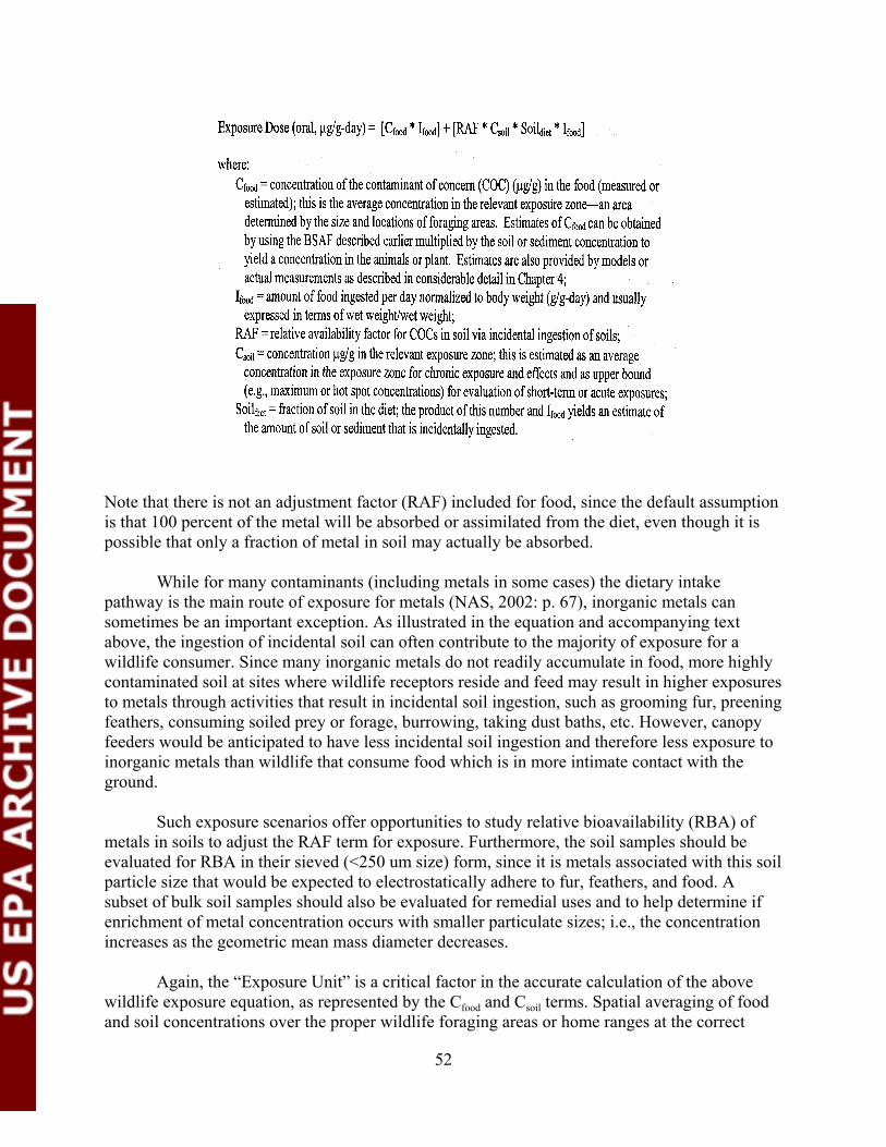
Note that there is not an adjustment factor (RAF) included for food, since the default assumption is that 100 percent of the metal will be absorbed or assimilated from the diet, even though it is possible that only a fraction of metal in soil may actually be absorbed.

While for many contaminants (including metals in some cases) the dietary intake pathway is the main route of exposure for metals (NAS, 2002: p. 67), inorganic metals can sometimes be an important exception. As illustrated in the equation and accompanying text above, the ingestion of incidental soil can often contribute to the majority of exposure for a wildlife consumer. Since many inorganic metals do not readily accumulate in food, more highly contaminated soil at sites where wildlife receptors reside and feed may result in higher exposures to metals through activities that result in incidental soil ingestion, such as grooming fur, preening feathers, consuming soiled prey or forage, burrowing, taking dust baths, etc. However, canopy feeders would be anticipated to have less incidental soil ingestion and therefore less exposure to inorganic metals than wildlife that consume food which is in more intimate contact with the ground.

Such exposure scenarios offer opportunities to study relative bioavailability (RBA) of metals in soils to adjust the RAF term for exposure. Furthermore, the soil samples should be evaluated for RBA in their sieved (<250 um size) form, since it is metals associated with this soil particle size that would be expected to electrostatically adhere to fur, feathers, and food. A subset of bulk soil samples should also be evaluated for remedial uses and to help determine if enrichment of metal concentration occurs with smaller particulate sizes; i.e., the concentration increases as the geometric mean mass diameter decreases.

Again, the “Exposure Unit” is a critical factor in the accurate calculation of the above wildlife exposure equation, as represented by the Cfood and Csoil terms. Spatial averaging of food and soil concentrations over the proper wildlife foraging areas or home ranges at the correct

52

exposure times of the year will provide appropriate food and soil concentration terms. Usually these spatial and temporal scales are selected to coincide with the respective toxicity benchmark (e.g., subchronic sampling based on reproductive endpoints in the feeding area of nesting birds). Other input factors such as area use and dietary fractions might need to be included in many exposure equations for more accurately estimating wildlife food chain exposures. Some examples of studies of bioavailability processes are shown in Table 4 (NAS, 2002).

4.3.3 Plants

The most common route of metal exposure in plants is through the roots. Ions and organic molecules contact roots via the transpiration stream, diffusive transport, and microbe-facilitated transport. At the root surface, soluble contaminants have the potential to enter into the root tissue through the transpiration stream or through a range of mechanisms that are designed to facilitate nutrient uptake. In general, it is thought that only uncomplexed, free ionic species of cations and ions can be taken up by roots. This has been described using a free ion activity model—FIAM (Lund, 1990; Parker and Pedler, 1997). However, exceptions to this model have been identified. Ionic or organometallic complexes that increase the total concentration of elements at the root surface have been correlated with increased uptake, either through disassociated ions or through uptake of intact complexes (McLaughlin et al., 1994: Parker et al., 2001). In addition, it is not clear how well plants can distinguish between ions of similar size and charge. The size of solid particles precludes their entry into plant roots, even for very small particles like colloids, such that contaminant release from the solid phase is a prerequisite regardless of the underlying uptake mechanism. Plant uptake of macronutrients is much better understood than uptake of micronutrients or contaminants, with the primary work on uptake of micronutrients focusing on iron (Welch, 1995). Different mechanisms have been identified that control macronutrient uptake by plants, providing a means through which contaminants can enter root tissue, as shown by the diagram below (NAS, 2002: p. 149).

Plant bioassays can be used to measure bioavailability processes (bioaccumulation factor, BAF) for a variety of compounds in soils. Two types of results can be generated, with the first providing a more accurate measure of BAF from co-located root-tip soil metals:

1) Plant tissue can be “directly” analyzed for BAF to determine if the contaminants of concern are present at elevated or potentially toxic levels. It is relatively straightforward to analyze plant tissue for concentrations of metals.

2) Measure BAF “indirectly” via the growth and vigor of plants (phytotoxicity). If the plant can grow in the presence of a contaminant, then one can conclude that the contaminant is not present in phytotoxic concentrations.

53

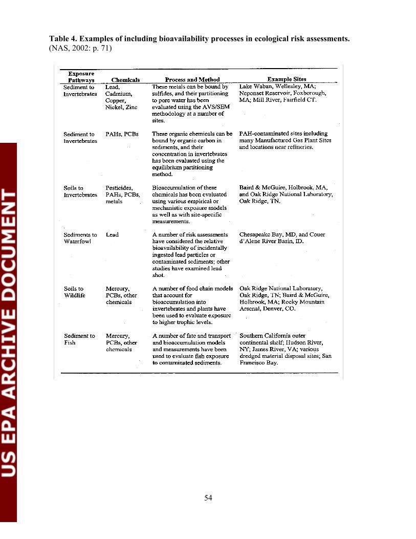
Table 4. Examples of including bioavailability processes in ecological risk assessments. (NAS, 2002: p. 71)

54

For both types of assays, the results can be used to determine either the direct or indirect value of bioavailability of contaminants in plants, and to extrapolate an indirect estimate of RBA to organisms that consume the plants (assuming a correlation between plant and animal uptake).

This type of testing has been routinely done in agriculture for decades and has been used to validate extraction tests. For example, growth tests are commonly used to better understand the bioavailability of herbicides, and tests that measure plant tissue concentrations are routinely conducted to evaluate plant nutrient status. Tests have most often focused on identifying plant deficiencies of particular elements, but are easily adapted to evaluate toxicities (Gettier et al., 1985). Plant uptake has been used to evaluate the effect of soil contamination as well as the ability of in situ treatments to reduce those effects (Pierzynski and Schwab, 1993; Chaney and Ryan, 1994; U.S. EPA, 1995a; Laperche et al., 1997). When used appropriately, plant tissue analysis can provide an indirect semiquantitative assessment of bioavailability processes. (NAS, 2002)

The utility of plant bioassays for measuring bioavailability of metals depends on the receptor (either the plant itself or a forager), as well as the particular metal, its route of uptake, and its potential mode of toxicity. For example, since zinc, nickel, copper, and manganese can cause phytotoxicity under field conditions, the potential toxicity to plants must be considered in evaluations of bioavailability for these elements to foragers. For other metals, concentrations in plants do not vary significantly, even with changes in soil concentration that span orders of magnitude. For certain other elements, consumption of enriched (metal accumulating) forages is the primary pathway through which these elements can enter the food chain and cause harm. In the latter case, plant tissue concentration is a viable means of measuring exposure to metals in higher organisms, even though plant yields may not be impacted by elevated metal concentrations in plant tissues. Specific examples of each of these cases follow.

Cadmium, lead, arsenic, chromium, and cobalt are usually not phytotoxic, even in cases of severe soil contamination in the field. Furthermore, lead, arsenic, chromium and cobalt are generally not taken up by plants in measurable quantities (Xu and Thornton, 1985; Chaney and Ryan, 1994; McGrath, 1995; Chaney et al., 2000). When these four metals have been found to be toxic to plants, uptake was generally confined to root tissues; thus, measurements of plant shoot concentrations would not be useful for risk assessments, since consumption of contaminated plant material is not a relevant exposure pathway for higher organisms.

For other elements, consumption of vegetation with elevated metal concentrations can be an important exposure pathway for consumers, although the metals are not phytotoxic. For example, consumption of plants containing elevated concentrations of cadmium has resulted in human fatalities (Kobayashi, 1978). In the case of selenium and molybdenum, uptake into the edible portion of plant tissues is generally not sufficient to cause plant toxicities but has lead to toxicities of animals consuming enriched plant tissue (Foy et al., 1978; Bingham et al., 1986; McGrath, 1995). Thus, measuring plant uptake of metals from soil is a means to evaluate metal exposure to higher organisms. It should be remembered when sampling plants as part of an ecological risk assessment that different wildlife species may feed on different plant parts at different seasons (which is also true for human risk assessments), resulting in differential accumulation of metals.

55

Plants are quite sensitive to manganese and zinc, with phytotoxicity of zinc being one of the primary concerns of excess zinc in soils. Because zinc kills plants at concentrations lower than those generally associated with adverse health effects in animals, phytotoxicity prevents zinc transfer from soil at toxic levels through the food chain (Chaney and Ryan, 1994). Plant zinc concentrations are also an effective measure of changes in bioaccessibility as a function of soil treatment with amendments, such that a reduction of plant tissue concentrations of zinc following an amendment is accepted as evidence of reduced environmental availability of the metal (Basta and Sloan, 1999; Brown et al., 2000).

As with any toxic endpoint, not a single metal concentration is associated with growth suppression and phytotoxicity across all plant species. For example, concentrations of zinc in plant tissue associated with phytotoxicity vary greatly both within and across species. Twenty varieties of soybean grown on the same high zinc soil, were found to have different uptake as well as yield responses (White et al., 1979). Four barley cultivars grown under identical conditions had zinc concentrations ranging from 52 to 126 mg/kg (Chang et al., 1984). Values for phytotoxic concentrations have been reported to range from 200 mg/kg (Bingham et al., 1986) to 500 to 1500 mg/kg (Chaney et al., 2000). For phytotoxic metal concentrations to be effectively used as an indirect measure of bioavailability, it is important that the threshold values of the plant tested are well understood. In addition, toxicities of certain metal elements are associated with deficiencies of others. For example, increased zinc, copper, and nickel toxicities can be associated with iron deficiencies (Bingham et al., 1986), while increased lead and zinc toxicities can also be related to phosphorus deficiencies (Laperche et al., 1997; Brown et al., 1999, 2000). Behavior of plant species in response to nutrient deficiencies varies, and this response can affect the uptake of potentially toxic metal elements (Marshner, 1998). Because of these multiple confounding factors, the bioavailability of metals in plants (as well as to consumers) is more accurately and reliably measured directly as the edible plant tissue concentrations of the metal in association with soil metal concentrations in the root zone (NAS, 2002, p. 248).

As with aquatic and lower terrestrial animals, the BSAF (biota soil/sediment accumulation factor) or BAF (bioaccumulation factor) can be used to measure the fraction of metal that is taken up into a plant from the environmentally available metal in the soil. This ratio or fraction is best expressed as a slope (assuming a linear or log-linear function) when tested over a gradient of soil concentrations, rather than derived from a narrow set of tissues and soil, and should include testing of relevant reference areas of soils and plants. Sometimes the dose- or concentration-response curves are U-shaped or flat, respectively, where apparent uptake ratios are greater at the lowest and highest concentrations of metals in soils compared to the middle concentrations of metals in soils, and where tissue metal concentrations remain stable over a wide range of soil metal concentrations. This discussion does not include comments on how soil physical/chemical characteristics affect BSAFs or BAFs.

Landscape plots with randomized subplot designs for sampling plant diversity and abundance plus phytotoxicity of metals may offer stronger scientific approaches for risk assessment (U.S. EPA 2000f; Henningsen 1998). Obtaining root-tip soil samples for co-location with plant metal concentrations is preferable to routine sampling that is taken for other purposes in risk assessments. Seasonal considerations in sampling are important for both phytotoxicity as well as for translocation of metals, which can change tissue concentrations by several orders of magnitude within weeks (U.S. EPA, 2000b). It is also critical to sample both the washed and

56

unwashed portions of plant tissues for metal analysis, because the washed portion can better reflect the BAF, while the unwashed portion may better represent the total exposure for consumers.

The proper edible portions of plants should be segregated for sampling to help evaluate exposures to consumers, while whole plants can be analyzed for tissue residues of metals for determining the BAFs. Noting the many confounding factors that can affect the uptake of metals in plants is important, especially as one attempts to adjust exposure estimates for consumers in food webs of risk assessments. Various confounding factors that should be considered in sampling plans and risk assessments include variations in climate, agricultural practices (irrigation—may cause leaching of metals; liming—may alter soil pH; grazing versus harvesting—may change plant growth physiology; mulching—may change TOC; fertilizer—may add phosphate salts or other metal anions to bind or precipitate metals, etc.); presence of accumulator (locoweed as Se indicators) or sensitive (alfalfa and Cu) plants; and plant senescence or seasonal effects (translocation of metals can occur from roots to edible stems and leaves). Cautious use for rough screening purposes only in risk assessments, should be made of generic literature BAFs for plants, such as those published by the Soil Conservation Service.

4.3.4 Soil Community: Invertebrates and Microorganisms

Metal speciation is the primary consideration in assessing the bioavailability/toxicity of metals to soil invertebrates and microbes in soil systems, whether it is at present time or some time in the future. However, major assumptions regarding metal exposure in aquatic systems, such as a the relatively homogenous dissolution of metals in the exposure water, may not be applicable or apply at different scales in soil systems. While soil microbes may be immersed in soil solution films surrounding soil particles, few invertebrates are exposed to metals in this manner. Exposure usually consists of partial contact of soil solution films with the surfaces of the invertebrates that are capable of absorbing metals (e.g., earthworm dermal surfaces). Direct contact with membranes across which metal uptake can occur does not take place for many soil invertebrates (e.g., arthropods), and metal uptake is almost entirely through the ingestion of metal associated with particulate matter or soil solution. For these reasons, exposure cannot be expressed similarly for each organism in the soil ecosystem, and an understanding of primary routes and mechanisms of metal exposure must be established for species or groups of similar organisms.

Understanding metal speciation, as determined by metal levels and soil physical/chemical characteristics, is a prerequisite for understanding any relationships between soil metal level and bioavailability/toxicity to soil-dwelling invertebrates/microbes. Three issues of understanding are necessary for linking metal speciation to bioavailability and toxicity in soil invertebrates and microbes:

1) Speciation as determined by chemists to define metal species in bulk soil solution and the intensity and capacity of metal species in solution.

2) Speciation as influenced by the biological surfaces and matrices (e.g., gastrointestinal tract, microbial surface) of organisms.

3) Speciation of metals in the organism and the effects on metabolism (i.e., speciation as related to metabolism, toxicity, and detoxification).

57

Metal species in bulk soil solution also need to be defined in terms of current potential toxic impacts (i.e., What metal species are organisms currently exposed to, and how should this be interpreted?) and short- and long-term partitioning/desorption behavior of metals (i.e., What metal species will be present in the exposure matrix in the next 10 months and the next 10 years, and how will this impact soil-dwelling organisms?). This may be better described in terms of intensity and capacity, with intensity defined as the amount of metal currently bioaccessible to the organism (e.g., pore water metal concentration or some surrogate measure), and capacity defined as the ability of the soil to replenish or maintain the concentration of metal in the pore water (i.e., short- and long-term desorption kinetics). Although intensity and capacity are concepts that are usually determined by soil chemists and models, understanding how soil invertebrates and microbes can modify the intensity and capacity of metals in soil systems is necessary.

Effects of Speciation (Bioaccessibility). In aquatic systems, metal speciation has a great impact on the bioavailability of metals for binding to gill membranes (Paquin et al., 2002), or as defined in this document, metal bioaccessibility by aquatic organisms. For soil-dwelling organisms, it is assumed that some metal species (e.g., divalent cations) are more bioaccessible than other metal species. However, little data exists on which metal species adsorb to surfaces of soil invertebrates and microbes, and which metal species are subsequently absorbed. Understanding which species of metals are available for sorption and uptake is fundamental for the development of a Biotic Ligand Model (BLM) for metals in soil systems.

Developing relationships between metal species present in soil pore water or a reasonable surrogate will form the basis of expressing the exposure dose for metals to soil invertebrates and microbes for the development of more accurate dose-response relationships. Due to the uncertain nature of metal speciation in soil systems and metal absorption and metabolism by soil invertebrates, an exposure dose-response relationship may still not be as accurate as using an internal metal burden in an organism for the development of dose-response relationships. In terms of expressing the exposure dose in a dose-response relationship for soil invertebrates and microbes, it is imperative to determine which chemical measure in the soil best describes exposure for a specific organism. Exposure dose can be expressed in a number of ways:

• Total metal (e.g., aqua regia digestion).

• Total environmentally available metal (e.g., weak salt extractable).

• Bioaccessible dose (e.g., theoretical portion that comes in contact with the surface of the organism and is available for sorption).

• Absorbed dose (e.g., actually taken up by organism).

In order to define metal exposure, metal measurements that would be useful in a model to predict metal effects to soil invertebrates and microbes can be categorized according to the metals speciation description provided previously. Specific measurements that would be needed include:

1) Metal speciation as determined by chemists to define metal species in bulk soil solution. This involves a sufficient characterization of the most important soil physical/chemical

58

characteristics that determine metal speciation (e.g., pH, organic C).

2) Metal speciation as influenced by the biological surfaces of organisms to determine the bioaccessible fraction of metals in soils. This would apply mostly to soil microbes that modify the environment immediately adjacent to their cell wall via exudates.

3) Pools of metals that are present internally in organisms (e.g., What ligands do metals form in organisms, and how are they detoxified?). This would apply mostly to soil invertebrates and would be more difficult to measure in soil microbes.

Metal Speciation in Soils. The various abiotic factors that affect metal speciation in soils are covered in the Environmental Chemistry issues paper. The Environmental Chemistry issues paper also provides some methods for determining metal speciation in soils.

Metal Speciation as Affected by Soil Organisms. Little information exists regarding the ability of soil microbes to modify metal speciation and toxicity in oxic soils. Similarly, little is known regarding the ability of soil invertebrates (e.g., earthworms) to alter metal speciation. Methods to evaluate effects of organisms on metal speciation in soil have not been developed, and it is not clear whether such research would provide a major contribution to our understanding of metal toxicity in oxic soils.

Metal Speciation within Soil Invertebrates. Once metals are absorbed, they are distributed to target tissues (sites of potential toxic action) and non-target tissues where the toxic interaction is non-existent or minimal and where detoxification can occur. The distribution of metals can differ for essential and non-essential metals. The distribution of absorbed metals and interactions with tissues is critical to our understanding of the potential toxic effects. Distribution should be examined both at the tissue/organ and subcellular level. In addition, due to competition of metals in absorption and metabolism, the absorption and distribution of large amounts of individual metals affects the mass and patterns of distribution of other metals (Scott-Fordsmand and Odegard, 2002). Such metal-metal interactions should be considered in all aspects of bioavailability and bioaccumulation.

The metabolism of metals determines the forms (species) that are present in organisms. Essential metal metabolism will be different from non-essential metals in that organisms will attempt to maintain a constant level of essential elements (e.g., Cu, Zn) regardless of whether external metal levels are deficient or elevated. Non-essential metals are more likely to accumulate to a level at which they cause toxic effects. Understanding the toxicodynamics of these elements will better aid in the development of specific biomarkers for their assessment.

Another area of metal metabolism that would be important in understanding the mechanisms of toxicity is examining the similarities and differences in metal exposure via dietary and external (waterborne) pathways. Metals absorbed from the intestinal tract are initially metabolized by digestive organs such as the intestine and hepatopancreas or similar structures. Metals that are bioaccessible to vascular tissues (e.g., earthworm epidermis) will be distributed to many tissues in general circulation.

Bioaccumulation and Biomagnification. Bioaccumulation of metals in soil invertebrates can be viewed as the net flux of metals into or onto an organism as a result of

59

absorption/adsorption, distribution, and excretion. Biomagnification of metals has not been generally observed to occur in soil invertebrates

Measures of Bioaccumulation

Bioaccumulation of hydrophobic organic compounds by soil organisms is typically described quantitatively by a biota-soil accumulation factor (BSAF), which is represented by the ratio of the chemical concentration in the organism to the chemical concentration in the soil and might be normalized for organism lipid content and soil organic carbon levels. Unlike bioaccumulation of hydrophobic organic compounds by aquatic organisms, bioaccumulation factors for metals by soil invertebrates are typically <1. However, these bioaccumulation factors (BAFs) are expressed as a ratio of total metals in the invertebrates to total metal levels in the soil sample. BSAFs expressed in this manner may be suitable for comparing metal bioaccumulation when the soil type is kept relatively constant (e.g., experiments conducted using artificial soil). However, for soils differing in metal bioavailability due to varying soil physical/chemical characteristics (e.g., pH, organic carbon, clay content), a BSAF expressed in this manner may not be suitable for comparing metal bioaccumulation. This may not be the best representation of metal bioaccumulation as it does not fully account for metal bioavailability in the soil system.

The whole body metal concentration in a soil invertebrate does represent metal bioavailability to the organism, but not all the metal in the soil is bioavailable to the organism. A ratio of total metal in the organism to some measure of the bioavailable fraction of metal in the soil (e.g., free ion concentration, weak salt extractable) may be more appropriate for expressing a BSAF, allowing a comparison of bioaccumulation of metals among different soils. Another approach to bioaccumulation was presented by Scott-Fordsmand and Odegard (2002) where earthworms exposed to various levels of Cu were analyzed by ICP spectroscopy to determine the concentrations of a wide range of metals. The patterns of metal accumulation varied with the Cu exposure concentration and could be separated using multivariate statistical approaches.

Models for Bioaccumulation

Bioaccumulation is typically modeled using a one-compartment, first order kinetics (1CFOK) model. Major assumptions of this model are (Spacie and Hamelink 1995):

1) Organisms are exposed to a constant concentration of chemical in the environment. 2) Uptake is proportional to the exposure concentration. 3) Every compartment within the organism is equally available for depuration. 4) Depuration follows first order kinetics.

Although this model may be applicable to hydrophobic organic contaminants in soil systems (Belfroid et al., 1995) and has also been used successfully for the bioaccumulation of some metals by soil invertebrates (Janssen et al., 1997; Conder et al., 2002), most of the assumptions of the model are violated when applied to bioaccumulation of metals by soil invertebrates. Soil invertebrates are not exposed to a constant concentration of metals in the soil over space and time. In fact, we are unsure of how to even express metal exposure, given that total metal concentration is inappropriate. We are not sure if uptake is proportional to exposure concentration since we cannot define the actual exposure concentration. Sufficient data exists on the metabolism of metals to show that all pools of metal taken up by the soil invertebrates are

60

not equally available for depuration; some are actually never depurated and are released only when the organism dies.

The 1CFOK model also assumes that the chemical concentration in the organism reaches a steady state that is proportional to the external concentration. Many studies have shown that this assumption is not valid for either essential or non-essential metals. Internal essential metal concentrations, such as Cu and Zn, are regulated and remain relatively constant over a wide range of soil metal concentrations. Although pseudo-first order kinetics may be observed in some situations, they generally do not apply to all metals. Only when normal regulatory mechanisms are overwhelmed do internal levels of essential metals increase. Accumulation of non-essential metals also violates the assumption of steady state for different reasons. Organisms have evolved mechanisms for the detoxification of non-essential metals that involve the internal accumulation of the metal in forms that are not toxic to the organism, such as incorporation into inorganic granules or binding to organic molecules to form metal ligands (e.g., metallothionein).

In many cases, accumulation of non-essential metals continues for the duration of exposure and/or the lifetime of the organism. In these cases, depuration rates, as defined in a 1CFOK model, are extremely slow or non-existent. Physiological mechanisms for the distribution and excretion of metals also differ among groups of soil invertebrates, so uptake and depuration kinetics are rarely similar among different groups of soil invertebrates. In practice, the assumptions of the 1CFOK model are indeed violated when examining the bioaccumulation of metals by earthworms (Eisenia andrei) and potworms (Enchytraeus crypticus) from different soils (Janssen et al., 1997; Peijnenburg et al., 1999a, 1999b). For some soils with some metals (e.g., Pb), 1CFOK was observed and a steady-state internal metal concentration was achieved. For other metals (e.g., Cu and Zn), internal levels rose rapidly and were maintained over a wide range of soil metal concentrations, suggesting regulation of these metals by the worms. For other metals, concentrations increased steadily and did not reach a plateau level.

For these reasons, the bioaccumulation of metals in soil organisms cannot reasonably be predicted. Questions that need to be answered in relation to metal bioaccumulation for soil invertebrates to allow the development of models for predicting metal bioaccumulation include:

1) How does metal bioaccumulation differ among different groups of soil invertebrates (e.g., Lumbricidae, Enchytraeidae, Isopoda, Collembola, Acaridae) with respect to metal uptake and depuration?

2) Are there taxonomic, physiological, or morphological relationships in metal metabolism that would allow us to group organisms together to allow the development of three or four general metal bioaccumulation models dependent upon how organisms metabolize metals?

3) What portions of the heterogeneous mixture of metals and soils do different groups of soil invertebrates “sample,” and do they modify their external environment to affect metal partitioning?

4) What chemical methods for metal measurement (e.g., pore water, free ion, weak salt extractable, total) are best correlated with metal bioaccumulation for the different groups of soil invertebrates?

61

Models for the prediction of metal bioaccumulation by soil invertebrates are primarily empirical in nature, describing relationships between metal body burdens in oligochaetes and collembola, soil metal concentrations, and soil physical/chemical characteristics. Statistical relationships have been established using univariate and multiple regression approaches. Peijnenburg et al. (1999b) established a monovariate regression formula for describing the quantitative relationship between log-transformed steady-state body concentrations of Cr, Cu, Ni, and Zn in Eisenia andrei and log-transformed total metal content of Dutch field soils (Peijnenburg et al., 1999b). Significant relationships were found for Cr, Cu, and Zn, with coefficients of determination of 0.61, 0.69, and 0.83, respectively. No significant relationship was found for Ni.

Peijnenburg et al. (1999a, 1999b) also derived multivariate regression relationships to describe uptake rate constants, steady-state concentrations, and bioaccumulation factors for Eisenia andrei and Enchytraeus crypticus as a function of soil characteristics. The soil parameters that generally contributed the most to explaining the variance between uptake rate constants and bioaccumulation factors were pH (for Cd, Zn), but also cation exchange capacity (CEC, for Pb) and clay content (for Cd). In general, the authors found that the effect of soil characteristics on metal bioaccumulation by Eisenia andrei and Enchytraeus crypticus was similar, suggesting that routes of metal uptake are similar within terrestrial oligochaetes. Similar studies are needed for describing relationships between soil physical/chemical characteristics and metal bioaccumulation in other groups of soil invertebrates such as Collembola and isopods.

Multiple regression models assume independence of the various parameters used to describe soil physical/chemical characteristics and do not consider covariation between parameters such as soil pH and clay content. Path analysis has been suggested as an alternative for multiple regression in describing these relationships and partitions simple correlations into direct and indirect effects, providing a numerical value for each direct and indirect effect and indicates the relative strength of that correlation or causal influence (Basta et al., 1993). Bradham (2002) used path analysis and backwards stepwise regression analysis to derive statistical models capable of predicting effects of As, Cd, Pb, and Zn on earthworm mortality, earthworm metal concentrations, and cocoon production based on soil properties. Both path analysis and backwards step-wise regression suggested that pH explained the greatest amount of variation in the effects of Cd, Pb, and Zn on earthworm mortality, with organic carbon also having a significant effect on Pb-induced mortality. Clay content was the only significant variable in explaining the variation in mortality of earthworms exposed to As.

Saxe et al. (2001) have described a model for predicting whole body concentrations of Cd, Cu, Pb, and Zn in Eisenia andrei as a function of pH, soluble metals in the soil at gut and environmental pH, and soluble organic carbon (SOC) in soil extracts. The model also included parameters that characterize the ability of worms to regulate the metal body burden, whether metal uptake is via the epidermal or gut surface, and whether the metal is essential. These models were very good at predicting metal accumulation from the Dutch field soils described by Janssen et al. (1997). The models also suggested that uptake of Cd, Cu, and Pb was almost exclusively across the epidermis and that only 18 percent of Zn uptake was across the gut.

Critical Body Residues and the Biotic Ligand Model. Critical body residues (CBRs) are an extension of the concept of bioaccumulation to internal concentrations of metals that are correlated with some toxic response, and hence represent toxicological bioavailability (Lanno et

62

al., 1998; Conder et al., 2002). CBRs in the appropriate species have been suggested to reduce uncertainties in ecological risk assessment procedures (Van Wensem et al., 1994; Van Straalen, 1996). Crommentuijn et al. (1994, 1997) and Smit (1997) established CBRs for sublethal effects for Cd and Zn, respectively, in Folsomia candida. Recently, Conder et al. (2002) examined the kinetics of Cd in Eisenia fetida exposed to Cd spiked in artificial soil at the level of the LC50. Worms were partitioned into two fractions by homogenization and centrifugation, and Cd kinetics was determined in each fraction. The idea here was to separate the total Cd pool in the earthworm into fractions representing toxicological bioavailability and a pool of detoxified Cd.

Cd in the two fractions exhibited different kinetics, with supernatant Cd increasing in a linear manner over the 16-day exposure period, and the pellet fraction exhibiting first order kinetics and reaching a steady state in about 4 days. The pellet fraction could represent a CBR as it was associated with the LC50 for the earthworms. Although empirical in nature, centrifugation/fractionation techniques have been used to separate metals in the various pools of invertebrates in order to isolate the fraction that correlates best with toxicity (Lanno et al., submitted; Jenkins and Mason, 1988). This approach takes into account the differences in metabolism between metals and organic compounds, where lipid is thought to contain most of the toxic organic compounds. If future research can isolate the fraction of an invertebrate that represents toxicological bioavailability, then it may be possible to estimate a toxicological biota-soil accumulation factor (TBSAF) representing a relationship between a specific fraction of metal that accumulates in the organism and a measure of chemical bioavailability in the soil.

In addition to the development of empirical models from primary laboratory data sets, researchers have developed more general models to estimate levels of metals in earthworms to be used in ecological risk assessment. Sample et al. (1999) developed a data base of soil and tissue concentrations of a number of metals (As, Cd, Cr, Cu, Hg, Mn, Ni, Pb, Zn) using total soil metal concentrations and total metal concentrations in depurated worms. Uptake factors and simple and multiple regression models of natural log-transformed concentrations of each metal in soil and earthworms were developed. Significant single variable regressions (soil metal concentration) were obtained for all metals except Cr. Inclusion of Ca as variable improved model fits for Cd and Pb, and the addition of pH only marginally improved model fits. The best general estimates of metal concentrations in earthworms were generated by simple ln-ln regression models for As, Cd, Cu, Hg, Mn, Pb and Zn, with no method accurately estimating Cr or Ni levels in earthworms.

Bioaccumulation represents the amount of metal adsorbed or absorbed by an organism from the bioaccessible metal encountered by the organism. The most accurate BSAF would represent the metal level in the organism and the metal bioaccessible to the organism, not the total concentration of metal in a volume of test soil. Somehow it is necessary to determine what portion of the test soil a soil organism actually encounters or samples. The assumption made in aquatic bioconcentration tests that the organism is exposed to a test medium with a constant, unchanging concentration of metal is not valid for soil test systems.

The premise and development of the biotic ligand model (BLM) in aquatic systems has been discussed extensively in section 4.1. Theoretically, a BLM could be developed for metal toxicity in soil systems for predicting metal toxicity to soil organisms. Models predicting metal speciation in soils would be needed and metal speciation must be correlated with some type of biotic ligand in a soil organism and an observed effect. The development of BLMs for soil

63

systems are being investigated (W. Peijnenburg, C.A.M. van Gestel, pers. comm.) and are still in their infancy.

Metal-Specific Effects Soil Invertebrates and Microbes. The effects of metals on soil invertebrates and soil invertebrate populations have been observed both in laboratory toxicity tests and in field studies. Although these effects were observed in relation to metals in these particular studies, these effects are not specific to metals. Biomarkers appear to be a more promising tool for assessing metal-specific exposure and effects in soil invertebrates. Biomarkers for metals can be classified according to whether they indicate exposure or effects and the level of biological organization at which they are measured, including cellular and subcellular (e.g., enzymes, metallothionein, genomics).

Specific to long-term metal exposure is the presence of inorganic granules containing high levels of various metals such as Cu, Cd, Pb, and Zn in various tissues, such as the hepatopancreas or chloragogenous tissues, of soil invertebrates (Morris and Morgan, 1986; Morgan and Morgan, 1998; Hopkin, 1989). The presence of granules is a clear indication of metal exposure, and determining the elemental composition of the granules can define to which metals exposure has occurred. However, this technique is not suitably quantitative for developing dose-response relationships.

The neutral red retention assay (NRRA) has been used as a biomarker of metal exposure in earthworms. This procedure involves examining the activity or amount of lysosomal enzyme that leaks through the lysosomal membrane after metal exposure. Coelomocytes from earthworms are exposed to neutral red, a supravital dye, for a specific time to allow uptake of the dye. Lysosomes in healthy cells permanently retain the dye but damaged lysosomes slowly leak the dye into the cytoplasm. The retention time of neutral red is negatively correlated with metal exposure and has been used to define good dose-response relationships with metal exposure in earthworms (Svendsen and Weeks, 1995; Scott-Fordsmand, 1998). Although dose-response relationships have been established with metal exposure, more research is needed to define how specific the response is to metal exposure or whether it simply suggests oxidative damage to lysosomal membranes.

Metallothioneins (MT) and other metal-binding proteins have been identified in many groups of soil invertebrates. The most thoroughly examined terrestrial invertebrate MTs are those of snails and slugs which are organ- and metal-specific and react differently when exposed to different metals (Dallinger, 1996). Some midgut isoforms of snails are induced rapidly by Cd and exclusively loaded with Cd (Berger et al., 1995), while other isoforms, such as Cu-MT, are non-inducible by either Cu or Cd (Dallinger et al., 1997). Metal-binding proteins have also been identified in earthworms, with some resembling MT in structure, while others are quite different, containing few cysteine and more aromatic amino acid residues (Morgan et al., 1989; Dallinger, 1996). MT and MT-like proteins in soil invertebrates provide a good measure of exposure to metals, but dose-response relationships are not clear, especially once toxicity is observed. The utility of MTs as a biomarker for metals would be restricted to exposure assessment with limited application for linkages to effects in organisms. However, MT-bound metals may be available for trophic transfer to predators, establishing this linkage with potential for trophic transfer.

Increased expression of other proteins, such as heat shock proteins (HSP), has been observed in response to metals exposure. However, these proteins are induced by a number of

64

environmental stressors and are not specific enough to prove useful in the assessment of metals exposure.

Promising biomarkers are being developed in the area of genomics, gene expression, and proteomics. These techniques involve measuring real-time alterations in specific messenger RNA. The underlying concept is that exposure to a particular chemical (e.g., Cd) will result in the transcription of messenger RNA sequences specific to proteins involved in the metabolism and/or detoxification of Cd. This may provide a chemical specific “fingerprint” for the type and quantity of chemical involved in the exposure. Microarray techniques where thousands of DNA sequences are sorbed to a glass slide, are being developed for Lumbricus rubellus (P. Kille, University of Cardiff, pers. comm.) and will be used in the near future for examining gene product responses of L. rubellus exposure to metals in soil.

Another approach to examining the expression of gene products is to separate and quantify proteins produced by the organism after exposure to metals. This proteomics approach is also currently being developed in soil organisms exposed to unexploded ordinances (UXOs) in soil (R. Kuperman, US Army, pers. comm.). Although both these techniques show considerable promise, they need to be validated with varying doses of different metals to determine if molecular responses are sufficiently specific to discriminate between exposures to different metals and doses. To date, most exposure have been in vitro in nature, with mammalian tissues exposed to different classes of compounds (e.g., heavy metals, various organics). These techniques have been able to discriminate between genetic responses to the different classes of compounds, and sometimes between doses of individual compounds. More validation of these techniques needs to be conducted in experiments where soil invertebrates are exposed in soils containing heavy metals. In conjunction, it is imperative to measure whole organism responses, the potentially bioaccessible metal fraction in the soils, and basic soil physical/chemical characteristics. Without the simultaneous measurement of all these parameters, model development for predicting metal bioavailability will not be possible, relegating genomics to the level of another biomarker of metal exposure that cannot be used to its fullest extent in ecological risk assessment or the development of regulations.

Application of Bioavailability in Soil Ecotoxicology. The major focus of applying bioavailability measurements in soil ecotoxicology is in determining the exposure dose of metals in soil that is best correlated with organism responses. In specific laboratory studies, total metal concentrations may prove a useful estimate of exposure dose, but when comparisons of toxicity among soils varying in physicochemical characteristics are made, total metal concentrations are often not predictive of toxicity. This is due to the effect of various modifying factors that alter the exposure dose by making metals less bioavailable to soil organisms. In site-specific risk assessments, alternatives to total metals, such as weak salt extractable metal levels, should be provided as estimates of metal exposure. For the development of national soil quality guidelines, laboratory data where exposure is based upon measures of potentially bioavailable metal levels in soil should be used to develop and express exposure dose.

4.4 Speciation: Its Role in Assessing Bioavailability in the Terrestrial Environment

The National Research Council (NRC) review on bioavailability (NAS, 2002) defined “bioavailability processes” in terms of three key processes. One of these processes, “contaminant interactions between phases,” is more commonly referred to as speciation. For a given metal or

65

metalloid, the term speciation describes a chemical’s ability to interact with its biological or chemical surroundings by characterizing its physicochemical properties that are relevant to bioavailability. Four toxicologically important determinants relate speciation to bioavailability:

1) Chemical form or species 2) Particle-size of the metal form 3) Lability of the chemical form 4) Source of metal

A wide variety of analytical tools have been used to characterize metal speciation as it is found to exist in various media. Currently, for risk assessment purposes (except for phytotoxicity), where large sites with numerous media, pathways, and metals must often be characterized in a reasonable time frame, electron probe microanalysis-scanning electron microscope (EMPA/SEM) techniques provide the greatest information on metal speciation. Other techniques such as extended x-ray absorption fine structure (EXAFS) and x-ray absorption near edge structure spectroscopy (EXANES) show great promise and will be important in solving key mechanistic questions. In the case of phytotoxicity, speciation of metals by direct measurement or chemical models of pore water chemistry is most valuable. Further work needs to be done in developing analytical tools for the speciation of the methyl-forming (Hg, As, Sb, Se, Sn) metals in soils and sediments.

4.4.1 Speciation

For a given metal or metalloid the term speciation refers to its chemical form or species, including its physicochemical characteristics that are relevant to bioavailability. Unlike organic compounds, metals do not degrade, but cycle through the environment in various forms or species. Bulk chemistry, TCLP (toxicity characterization leaching procedure), or SLP (soluble leaching procedure) concentrations for any metal provide neither sufficient chemical information to understand the environmental behavior of a metal nor to develop remedies for its safe management. Although these tests are essential for site characterization and management, they offer no insight into risk. Rather, the speciation and bioavailability of a metal play a significant role in the risk assessment of contaminated media.

The NRC review on bioavailability (NAS, 2002) defined “bioavailability processes” in terms of three key processes:

1) Contaminant interactions between phases—(Association-Dissociation/Bound-Released) 2) Transport of contaminants to organism 3) Passage across physiological membrane

This first process, contaminant interactions between phases, has more commonly been termed speciation. Determining the species of a toxic metal in the environment is a critical component of any health risk assessment. The concept of speciation describes the ability of a metal to interact with its biological or chemical surroundings by characterizing its physicochemical properties. The four toxicologically important determinants that relate speciation to bioavailability (chemical form or species, particle-size, liability, and source) will discussed in more detail below.

66

Chemical Form or Species. The solid phase in a medium that controls the activity of a metal in solution, whether the solution be surface/ground/pore water or gastrointestinal fluids, plays a profound role in metal bioavailability. Studies have shown that metal species found in a solid medium are often diverse, and data suggest that the bioavailability may be significantly influenced by site-specific variations in identified metal species (Davis et al., 1993; Ruby et al., 1992; Drexler, 1995, 1997).

Particle-Size of Metal Species. Particle-size of a metal form is an important factor in the mobilization of the metal ions. This is primarily the result of a relative increase in the surface area to mass of the particle, as the geometric mean diameter size decreases, ultimately yielding an increase in solubility of the metal. Thus, although solubility is not the only control for bioavailability, a decrease in particle size has been directly attributed to an increase in bioavailability—presumably through increased dissolution of the metal. Barltrop and Meek (1979) observed that “the smaller the lead particle, the higher blood lead level.” Similar observations were made by Healy et al. (1982) using galena (PbS) and an in vitro dissolution technique. Drexler (1997) presented in vitro results on numerous lead-bearing phases ranging in particle size from 35 to 250 microns and showed an increase in Pb bioavailability with decreasing particle-size; more significantly, not all forms showed the same magnitude of change. Finally, such laboratory data have been corroborated by extensive epidemiological evidence, supporting the importance of particle size on bioavailability (Bornschein et al., 1987; Brunekreef et al., 1983; Angle, 1984).

Lability of Particle. The impact of the lability of a metal particle or its strength associations within a medium matrix, on bioavailability is not well documented, but it follows the theoretical premise put forth by many of the developing, treatment technologies—to be bound or relatively isolated from the environment. Data from several EPA Superfund sites and from Region 8 swine studies suggest that matrix associations, such as liberated versus enclosed particles of metals, can play an important role in bioavailability. Two different media with similar total lead concentrations and lead forms (slag, lead oxide, and lead arsenate) can exhibit significantly different bioavailabilities. In situ observations can be very useful in understanding the mechanistic phenomena controlling bioavailability. In addition, such data on the liability of metal in particles will aid in the development and validation of models used to predict metal interactions with their environment.

Source of Metal. Although the source of a metal is not directly related to bioavailability, it does play an important role in risk assessment by evaluating pathways, background, and apportionment. It is important to understand the pathways of exposure and transport of a metal before any remedial action can be taken; otherwise, recontamination of the primary pathway and reexposure can occur. A knowledge of background metal levels is required by federal statute, as an action level cannot be established below natural background levels. Finally, cost recovery can be an important factor in a remedial action, as it is the responsibility of the agency to identify and, if possible, to seek the assistance of responsible parties to address sources of metal contamination. Source can play a more direct role in bioavailability, especially for ecological receptors and in human risk analyses when multiple exposure pathways through diet and nondietary sources exist, or when background metal levels can contribute substantially the receptor exposure—thus confounding the determination of bioavailability.

67

4.4.2 Tools

A wide variety of analytical and chemical techniques have been used to characterize metal speciation in various media (Hunt et al., 1992; Manceau et al., 1996, 2000; Welter et al., 1999; Szulczewski et al., 1997; Isaure et. al., 2002; Lumsdon and Evans, 1995; Gupta and Chen, 1975; Ma and Uren, 1995; Charlatchka et al., 1997). These techniques must provide information on speciation, particle size, and the source of the metal and also quantitatively determine the metal level present. Of the techniques tested (physicochemical, extractive, and theoretical), the tools that have been used most often to evaluate speciation include:

Particle-Bound Metal:

XAS X-ray absorption spectroscopy XRD X-ray diffraction PIXE and µPIXE Particle induced x-ray emission EPMA-SEM Electron probe microanalysis-scanning electron microscopeSIMS Secondary ion mass spectrometryXPS X-ray photoelectron spectroscopy

Sequential extractions Single chemical extractions

Over the past decade, numerous advances in materials science have led to the development of a wide range of analytical tools for determining metal concentrations, bonds, and valences of individual particles on a scale that can be considered useful for the speciation of environmentally important materials (soils, wastes, sediments, and dust). Although most of these tools are scientifically sound and offer important information on the mechanistic understanding of metal occurrence and behavior, only a few provide currently useful information on metal bioavailability for use at a “site” level (see Table 5). However, one may still find other techniques to be essential for conducting a detailed characterization of a selected material to describe the chemical or kinetic factors controlling the release, transport, and/or exposure of a metal.

An indirect approach to speciation, compared to the direct methods previously described, include the functional or operational extraction techniques that have been used extensively (Tessier and Campbell, 1979, 1988; Gupta and Chen, 1975). These methods use either a single or sequential extraction procedure to release species associated with a particular metal within a medium.

Single chemical extractions are generally used to determine the bioavailable amount of metal in a functional class (e.g., water-soluble, exchangeable, organically bonded, Fe-Mn bound, or insoluble). In a similar approach, sequential extractions treat a sample with a succession of reagents that are intended to specifically dissolve different and less available phases. Many of these techniques are a variation on the classical method of Tessier et al. (1979), in which metal associated with exchangeable, carbonate-bound, Fe-Mn bound, organically bound, and residual species are determined. A number of excellent reviews on the use and abuse of extraction techniques are available (Beckett, 1989; Kheboian and Bauer, 1987; Foerstner, 1987). These techniques can be useful in a study of metal uptake by plants and soil invertebrates, where transfer takes place predominantly from a water solution phase. However, one must keep in mind that these methods are not “selective” for metal species, and above all, these leachable fractions have never actually been correlated to bioavailability.

68

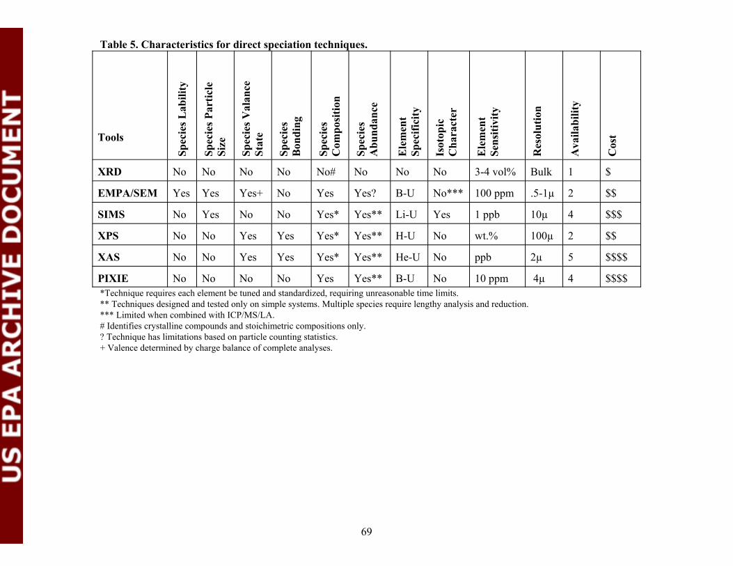
Tools

XRD No No No No No# No No No 3-4 vol% Bulk 1 $

EMPA/SEM Yes Yes Yes+ No Yes Yes? B-U No*** 100 ppm .5-1µ 2 $$

SIMS No Yes No No Yes* Yes** Li-U Yes 1 ppb 10µ 4 $$$

XPS No No Yes Yes Yes* Yes** H-U No wt.% 100µ $$

XAS No No Yes Yes Yes* Yes** He-U No ppb 2µ $$$$

PIXIE No No No No Yes Yes** B-U No 10 ppm 4µ 4 $$$$

2

5

Spec

ies L

abili

ty

Spec

ies P

artic

le

Size

Spec

ies V

alan

ce

Stat

e

Spec

ies

Table 5. Characteristics for direct speciation techniques.

Spec

ies

Com

posi

tion

Spec

ies

Abu

ndan

ce

Ele

men

t Sp

ecifi

city

Isot

opic

C

hara

cter

Ele

men

t Se

nsiti

vity

Res

olut

ion

Ava

ilabi

lity

Cos

t

*Technique requires each element be tuned and standardized, requiring unreasonable time limits.B

ondi

ng** Techniques designed and tested only on simple systems. Multiple species require lengthy analysis and reduction. *** Limited when combined with ICP/MS/LA.# Identifies crystalline compounds and stoichimetric compositions only.? Technique has limitations based on particle counting statistics.+ Valence determined by charge balance of complete analyses.

69

Solution Speciation (Computer-Based Models). Computer-based models are either based upon equilibrium constants or Gibbs free energy values in order to determine metal speciation from solution chemistry conditions (concentration, pH, Eh, organic complexes, adsorption/desorption sites, and temperature). Both approaches are subject to mass balance and equilibrium conditions that must be controlled. These models have undergone a great deal of development in recent years, as reliable thermodynamic data have become available and can provide some predictive estimates of metal behavior. A good review of these models and their applications is provided by Lumsdon and Evans (1995). Examples of computer-based speciation models include MINTEQL, REDEQL2, ECOSAT, MINTEQA2, HYDRAQL, PHREEQE, and WATEQ4F.

In some instances, metal speciation may be controlled by simple reactions. However, in many cases, (particularly in contaminated media) the state of equilibrium and reversibility of metal reactions are unknown. In addition, these mathematical thermodynamic equilibrium models suffer from other limitations:

• Lack of reliable thermodynamic data on relevant species • Inadequacies in models to correct for high ionic strength • Poorly known reaction kinetics • Complex reactions and lack of models for co-precipitation/adsorption

This first limitation is perhaps the most significant for contaminated media. As an example, none of the models would predict the common, anthropogenic, lead phases of paint, solder, or slag.

Plants. When considering the bioavailability of a metal to plants from soil and sediments, it is generally assumed that both the kinetic rate of supply and the speciation of the metal to either the root or shoot are the most important factors. In soils and sediments, there is generally a small volume of water in contact with the chemical form of the metal. Although the proportion of soluble metal in pore water is small compared to the bulk soil/sediment metal concentrations, it is this phase in pore water which is directly available to plants at the root tips. Therefore, understanding porewater chemistry is critical; that is, measuring metal concentrations as simple inorganic species, organic complexes, or colloid complexes is most important.

Tools currently used for metal speciation in plants include:

• In situ measurements, using ion selective electrodes (Gundersen et al., 1992; Archer et al., 1989; Wehrli et al., 1994).

• In situ collection techniques using DET (diffusive equilibrium thin films) and DGT (diffusive gradient thin films) followed by laboratory analyses (Davison et al., 1991, 1994; Davidson and Zhang, 1994; Zhang et al., 1995).

• Equilibrium models (SOILCHEM) (Sposito and Coves, 1988).

4.5 Predictive Assays for Terrestrial Mammals

Measurement of metal bioavailability in animals or humans and plants has a number of potential benefits, but it also can be a relatively slow and costly process when compared to potential lab methods (if validated), plus the conduct of in vivo studies may not be a feasible option in all cases. For these reasons a number of scientists have worked to develop alternative

70

in vitro procedures that may provide faster and less costly alternatives for estimating the relative bioaccessibility of a metal in soil or soil-like samples (Miller et al., 1982; Imber et al., 1985; Ruby et al., 1993; Ruby et al., 1996; Medlin 1997; Rodriquez et al., 1999; Drexler et al., 2003). These methods are based on the concept that the rate and/or extent of metal solubilization in the gastrointestinal fluid is likely to be an important determinant of metal bioavailability in vivo, and most in vitro tests are aimed at measuring the rate or extent of metal solubilization in an extraction solvent that resembles gastric fluid. Based on a review of all methods, it is clear that bioaccessibility for certain metals can be determined using an in vitro method with reasonably high precision and accuracy. Only two in vitro methods (Medlin, 1997; Drexler et al., 2003) establish a defensible bioequivalency with in vivo models of bioavailability for metals.

The incidental ingestion of contaminated soil is the most significant pathway of exposure to metals in humans (Calabrese et al., 1987; Barltrop, 1973; Mushak, 1991; U.S. EPA, 1989b). However, even though a completed exposure pathway is established, uptake can be altered as a result of social (Casteel et al., 1997), biological (Mushak, 1991), or physicochemical (Van Borm et al., 1988; Davis et al., 1993; Drexler, 1995) factors. These chemical and physical properties of the soil medium tend to influence (usually decrease) the bioavailability of the metal when ingested. Thus, equal ingested doses of different forms of metal in different soils or media may not have the same bioavailability and so would not pose equal health risks. Studies now indicate that metal bioavailability may span a wide range of values for certain metals (U.S. EPA, 2002b; Drexler et al., 2003). Therefore, an accurate estimate of bioavailability of metals, prior to the evaluation of potential human health risk is essential for reducing uncertainty and for accurate risk-based decision-making.

Historically, bioavailability has been estimated based on either 1) experimental animal models (in vivo), 2) validated toxicokinetic models, or 3) epidemiological studies. These methods are generally complex, slow, expensive, and thus often limited in application to large sites that often exhibit wide ranges of variability in bioavailability. In vitro testing, on the other hand, can be simple, rapid, and inexpensive; however, these tests cannot reflect the complex physiological or pharmacokinetic aspects of human absorption. Therefore, in order to be scientifically defensible, an in vitro/in vivo correlation (IVIVC) must be developed and validated; that is, a bioequivalence must be established.

Physiology of the GI Tract. In order to evaluate the bioavailability of metals by the human body through digestion, numerous factors must be considered. A precursor to understanding the dissolution and absorption process is to be familiar with the fundamental structure and chemical environment of the digestive system.

Digestion of material entering the oral cavity begins in the mouth. Saliva is excreted continuously throughout the day (1 to 2 liters), and its pH ranges from 6.2 to 7.4, depending on the amount and type of food present, but pH values as low as 3 can be produced around the teeth by the action of bacteria. Transit in the mouth is so short (10 to 20 seconds) that little to no digestion occurs other than the mechanics of particle-size reduction by the teeth. From the mouth, food is transported to the stomach via the esophagus (25 cm long). The pH of the esophagus is between 6 and 7, in which the majority of the fluid present is from saliva. Transit time is very short, from 10 to 14 seconds.

The stomach is a reservoir for food, secreting acid and pepsinogen as it processes food into chyme and begins to digest proteins. The volume of gastric fluid produced on a daily basis by the stomach is approximately 1 to 1.5 liters. The pH of the fluid averages 2.7 over a 24-hour

71

period. However, positionally within the stomach or during times of fasting, gastric pH can range from 1.6 to 4.5. Stomach pH is generally lowest early in the morning, and men have a slightly lower basal pH (2.16) than do women (2.79). No significant difference in gastric pH has been observed with age. Hydrochloric acid, the primary component of gastric juice, is secreted at a rate of between 60 to 200 ml/hr in the average adult. Secretion continues until all food has left the stomach.

When food is ready to leave the stomach, it passes to the small intestine through the pyloric sphincter. Pancreatic and bile ducts open into the small intestine at a point very near the pylorus. The alkaline content of pancreatic and biliary secretions neutralizes the acid of the chyme and changes the pH to slightly alkaline (pH 7 to 8). The small intestine is the longest section of the GI tract, extending from the duodenum to the ileum, approximately 5 to 6 meters in length. The prominent feature of the small intestine is the elaborate folding of the epithelium, villi and microvilli, producing a usable surface area of approximately 200 m2 in the average adult, (Washington et al., 2001) thus providing an optimum environment for digestion and absorption. Approximately 2 to 3 liters of fluid are secreted from these sources in an average day, with a pH between 7.5 and 8.

By the time ingested material enters the large intestine, more than 80 percent of the dietary and secreted fluid has been absorbed along with most nutrients. Transit times within the small intestine vary from minutes (in the duodenum) to more than 12 hours in the lower portions. Some metals are absorbed, including sodium, calcium, iron, cobalt, zinc, mercury and lead (Bezwoda et al., 1978; Endo et al., 1986; Henning and Cooper, 1988). The ileum, the anterior section of the small intestine, is the primary site for nutrient absorption. The jejunum is the distal section of the small intestine, and after leaving the jejunum, undigested food material passes into the large intestine. Along this approximately 125 cm route, a pH of 6.4 to 7.0 is maintained while water and electrolytes are absorbed, producing a solid stool for defecation. Total transit time for the large intestine ranges from 7 to 14 hours.

Biological Mechanisms of Metal Uptake. The biochemical factors that influence gastrointestinal absorption of most metals are complex, and the reader is directed to Morton et al. (1985) and Mushak (1991) for a more complete review. The epithelial lining of the small intestine is the principal site of uptake and transport of dissolved metals from the lumen. Experimental studies indicate two primary transepithelial interactions between metal solutions and intestinal epithelium: 1) active transport and 2) passive transport mechanisms. Active transport is enzymatic and cofactor based, a mechanism that is saturable and therefore rate-limited for transport, and it is thus more significant at low concentrations of metals. Passive transport can be “carrier-mediated” transport, such as illustrated by the protein ferritin and its role in the uptake of iron (Adams et al., 1991) or with cysteine and the uptake of zinc (Hempe and Cousins, 1992). Metal uptake can also take place by simple diffusion through small pores (10 to 16 D) in the tight junctions between adsorptive cells (Morton et al., 1985). Pinocytosis of small particles also occurs by phagocytic cells in the small intestine.

In Vitro Model Design. Model development has focused on the simulation of complex physiological and biological functions within the GI tract, including considerations of:

• pH. • Solid/liquid ratios. • Motility/transit.

72

• Solution chemistry instead of establishing a bioequivalence between in vivo and in vitro results.

The two-solution method has been most common addressing pH changes in the GI tract, providing an exposure to both the low pH of the stomach (methods pH ranging from 1.3 to 3.0) and the higher pH of the intestine (5.5 to 7.0) (Table 6). Solution pH is usually maintained either by titrations with drop-wise addition of acid or base while solutions are continuously monitored or using buffers.

The solid:fluid ratio used for in vitro models has ranged from 1:10 to approximately 1:150 (g/ml) (Table 6). None of these reflects the 2:1 ratio observed in adults (3000 g daily food intake versus the 1500 ml stomach volume) (Washington et al., 2001). It is recommended that this ratio be dictated by practical considerations. Therefore, a sample mass should be provided that can be accurately weighed and is representative, along with a volume that can help maintain good particle to solution contact and minimize any unusual kinetics.

The motility and transit time within the GI tract is difficult to model with standardization. Both processes vary greatly within the GI tract and can be affected by diet and daily cycles. Historically, authors have used either diffusers, stirrers, or rotation devices to mimic these factors. All methods are adequate; however, the diffuser system is difficult to control and clean. Also, rotation mechanisms are not favorable to techniques which require constant pH monitoring.

Variations observed in extraction fluid chemistry are by far the greatest source of method deviations. Although most methods have the gastric solution dominated by HCl, other acids, proteins, and peptides have been added with extraction times of about one hour. Intestinal solutions have their pH adjusted by addition of sodium bicarbonate and/or other biological salts and are extracted for 3 to 5 hours. Most systems were maintained at a temperature of 37°C and some methods used argon to maintain anaerobic conditions, even though the GI tract is aerobic in humans.

73

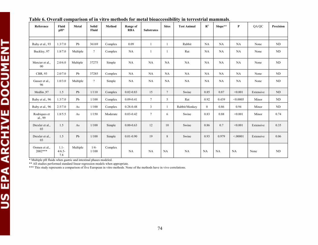
Table 6. Overall comparison of in vitro methods for metal bioaccessibility in terrestrial mammals. Reference Fluid

pH* Metal Solid/

Fluid Method Range of

RBA Substrates Sites Test Animal R2 Slope** P QA/QC Precision

Ruby et al., 93 1.3/7.0 Pb 36169 Complex 0.09 1 1 Rabbit NA NA NA None ND

Buckley, 97 1.8/7.0 Multiple ? Complex NA 1 1 Rat NA NA NA None ND

Mercier et al., 00

2.0/6.0 Multiple Simple NA NA NA NA NA NA NA None ND

CBR, 93 2.0/7.0 Pb 37285 Complex NA NA NA NA NA NA NA None ND

Gasser et al., 96

1.0/3.0 Multiple ? Simple NA NA NA NA NA NA NA None ND

Medlin ,97 1.5 Pb 1/110 Complex 0.02-0.83 15 7 Swine 0.85 0.87 <0.001 Extensive ND

Ruby et al., 96 1.3/7.0 Pb 1/100 Complex 0.09-0.41 7 5 Rat 0.92 0.439 <0.0005 Minor ND

Ruby et al., 96 2.5/7.0 As 1/100 Complex 0.28-0.48 3 1 Rabbit/Monkey 0 0.86 0.94 Minor ND

Rodriques et al., 99

1.8/5.5 As 1/150 Moderate 0.03-0.42 7 6 Swine 0.83 0.88 <0.001 Minor 0.74

Drexler et al., 03

1.5 As 1/100 Simple 0.00-0.63 12 10 Swine 0.86 0.7 <0.001 Extensive 0.35

Drexler et al., 03

1.5 Pb 1/100 Simple 0.01-0.90 19 8 Swine 0.93 0.979 <.00001 Extensive 0.06

Oomen et al., 2002***

1.1-4/6.5-

7.8

Multiple 1/4-1/100

Complex NA NA NA NA NA NA NA None ND

37275

* Multiple pH fluids when gastric and intestinal phases modeled. ** All studies performed standard linear regression models when appropriate. *** This study represents a comparison of five European in vitro methods. None of the methods have in vivo correlations.

74

Evaluation of In Vitro Methods. Bioequivalency tests that an in vitro dissolution test must be both discriminatory and reproducible. To meet these objectives, a useful in vitro method must provide the following:

• An In Vivo–In Vitro Correlation (IVIVC) • A method validation • Quality Assurance/ Quality Control (QA/QC) • A sensitivity analysis

Correlation:

It is imperative that a scientifically acceptable in vitro method be significantly correlated with an in vivo/in vitro method that is based upon:

• An acceptable animal model • Its regression parameters • The range in RBA from in vivo results • Variety of mineralogical metal forms tested.

Numerous animal models have been used to produce in vivo estimates of metal bioavailability: rabbits, mice, rats, dogs, swine, monkeys, and, in a few instances, children and adult humans. However, at the present time, juvenile swine (LaVelle et al., 1991) are the model accepted by EPA for the determination of lead and arsenic bioavailability. To ensure the in vitro method is discriminatory, it is very important that the correlation be based on a wide-range of in vivo RBA estimates based upon large numbers of tested substrates.

Validation:

To further assess the quality of the method, both a inter- and intra-laboratory validation should be performed. The interlaboratory validation will provide important information on the precision of the method, while accounting for analytical, procedural, and operator bias. The intralaboratory study will independently validate the work and dictate the repeatability of the method as a potential industry standard.

QA/QC:

Following Good Laboratory Practice (GLP) (Federal Register, 1989c), the in vitro method should provide a quality assurance/quality control (QA/QC) protocol. The protocol should include a method with standard operating procedures (SOPs), along with blanks, spikes (matrix and blank), duplicates, and traceability (chain of custody), plus criteria for frequency, acceptability and corrective action.

Sensitivity:

The final criterion used to assess the quality of an in vitro method is a sensitivity analysis; it can often explain why a method is not reproducible or discriminating. It is important to understand how the IVIVC is affected by variations in the components of the method.

75

Components to be evaluated should include, but may not be limited to, solid/liquid ratios, pH, temperature, gastric/intestinal and simple/complex, time, and post extraction stability.

Conclusions. A number of in vitro methods have been developed for the estimation of metal bioaccessibility in the human gastrointestinal tract (Table 6). These methods illustrate a broad range in scientific complexity but most have very limited scientific defensibility. Based on careful reviews of these methods, it is clear that bioaccessibility for certain metals can be determined using a validated in vitro approach, capable of attaining high precision and accuracy. Since the data derived from these methods may require and produce different levels of scientific quality, a number of the available methods may or may not meet the user’s needs for estimating bioaccessibility of metals in risk assessments. Only four of the eight methods produced an IVIVC, and only two methods (Medlin, 1997; Drexler et al., 2003) established a defensible bioequivalency. Therefore, only these latter two are recommended for quantitative risk analyses.

5. FUTURE DIRECTIONS TO IMPROVE CURRENT AGENCY PRACTICE

5.1 Aquatic-Based Assessments

Bioavailability and bioaccumulation of metals in aquatic systems are of prime importance in the context of reducing uncertainty in metals assessments because they are the mechanistic link between exposure and effects. The discussion in previous sections clearly highlights the complexity of assessing and predicting the bioavailability and bioaccumulation of metals in aquatic systems. This complexity arises from many factors including:

• Essentiality of some metals resulting in a “U”-shaped dose response curve. • Variation in assimilation efficiency for different species of metal, for different biota and at

different sites of uptake. • Ability to modulate uptake at the various sites of uptake. • Contributions of different routes of entry to the metal body burden and effects. • Ability to sequester, store, detoxify and eliminate bioaccumulated metals. • All metals will bioaccumulate to some degree without impacts as a result of exposure to

natural background concentrations.

Incomplete characterization of these and other complexities contributes to uncertainty in the assessment of metals, and these uncertainties can be amplified in assessments that involve applications across multiple geographical scales, receptors, and metal compounds.

Much progress has been made over recent years in refining the understanding of the geochemistry of metals in aquatic systems in relation to bioavailability and how this can be applied to reduce the uncertainty by explaining the variability observed in toxic responses. Modeling approaches such as the free ion activity model (FIAM) and the biotic ligand model (BLM) have been shown to offer significant improvements over hardness equations in linking exposure and acute impacts. Although not without its own set of limitations, the BLM has a mechanistic basis and considers not only the abiotic factors that affect bioavailability but also, at least conceptually, bioaccumulation. Although considerable advances have been made in understanding the mechanisms of metal bioaccumulation in biota, these have not yet contributed

76

substantially to reducing uncertainty. Arguably, from the regulatory context, the increased understanding of metal bioaccumulation has revealed more uncertainty than it explains.

Therefore, an obvious and important question is:

How (and to what extent) can the existing and emerging body of science pertaining to metal bioavailability and bioaccumulation be used to reduce uncertainty in the Agency’s metals assessments?

This is a particularly challenging question to address given the large volume and incomplete coverage of the metals literature, the complexity of the bioaccumulation process, and the diverse scope of the Agency’s assessment types (e.g., broad scale hazard classifications, national risk assessments, site-specific risk assessments).

Ultimately, to reduce uncertainty in metals assessments, more robust connections need to be established between the bioavailable form(s) of metals in various exposure media, their accumulation, metabolism and distribution in tissues, and the form(s) of metals that exert their toxicity directly to the organism or indirectly to its consumers. However, for many metal-organism combinations, data are lacking on the mechanism(s) of action (e.g. the site(s) of toxic action, the metal form(s) responsible for eliciting effects, the mechanisms and pathways for detoxification and storage and kinetic aspects of uptake, elimination, and metabolism), and these need to be understood in order for bioavailability and bioaccumulation models to improve linkages between exposure and effect or accumulation and effect.

Therefore, there is significant uncertainty as to the extent which total metal measurements in tissues of aquatic organisms (the format of most metal residue data) provide meaningful exposure metrics for estimating risk from direct or indirect (i.e., trophic transfer) toxicity. The steps taken to solidify the exposure-bioaccumulation-toxicity relationship should reflect the specific nature of various metal exposure-to-receptor scenarios and effectiveness of existing Agency programmatic controls, so that both uncertainty and risk reduction efforts are targeted and maximized. It is important that research to fill these data gaps be specifically focused so as to ensure the efficiency of resource expenditures. For example, future steps to improve our characterization and prediction of trophic transfer should target those metal-receptor scenarios where the uncertainty of trophic transfer is likely of greatest importance in the context of existing Agency programs.

Moving from the current situation to a revised, improved, and validated set of criteria and/or methodologies for assessing metal hazards and risks presents a number of options and challenges, as currently there would appear to be no clear alternatives ready for application. Because the processes of environmental assessment and scientific development is ongoing, the Agency should consider a flexible and interactive approach while developing and optimizing its Metals Assessment Framework. The ultimate goal would be to provide scientifically rigorous and validated methodologies and to address all possibilities. To achieve this, a variety of considerations and suggestions must be addressed and balanced in a complete, but also pragmatic and ongoing manner, as research results and consensus become available.

77

For example, not only has the use of BAFs and BCFs for hazard assessment of metals been challenged, but so has the concept of metal bioaccumulation itself. Even though this issue needs to be addressed, it must also be recognized that bioaccumulation is currently used for hazard-based assessments, and, therefore, solutions must be both scientifically and pragmatically based. As well, the concept of bioaccumulation is sound for use in assessing risk of metals for which effects can be expressed through residue-based mechanisms. However, with many metal-organism combinations, available data and tools do not characterize the bioavailability or bioaccumulation process with sufficient rigor to enable unambiguous predictions of metal residues that are toxicologically meaningful for evaluating impacts to aquatic organisms. In the case of direct toxic impacts, the rates of metal accumulation are perhaps more meaningful than tissue residues (the BLM being an exception with acute toxicity), while for indirect toxicity, the form of the bioaccumulated metal and internal distribution in prey organisms as well as the feeding ecology of the consumer are key factors for consideration in addition to the metal burden of prey.

Perhaps a more effective way is an organized and tiered transition moving from current applications to revised methodologies, with each phase providing additional reductions in uncertainty as the increasingly sophisticated scientific understanding of bioavailability and bioaccumulation is incorporated. The framework should therefore be sufficiently flexible to incorporate these transitions over time. With these considerations in mind, the following are some of the recommendations and concepts that may help to shape directions that can be included in the developing Metals Assessment Framework and other related actions in the context of metals bioavailability and bioaccumulation to aquatic organisms.

Use and Interpretation of Aquatic Bioaccumulation Data. Current Agency practice relies extensively on the use of aquatic BCF/BAF data for estimating and predicting the bioaccumulation potential of metals and metal compounds. Use of BCF/BAF data span the range of assessment types, including hazard classifications, national assessments, and site-specific assessments. The substantial quantity and availability of BCF/BAF data, combined with the relative simplicity in which these data can be incorporated into risk assessments undoubtedly contribute to their widespread use. However, data and uncertainties revealed in previous sections have important implications for the use and interpretation of metals bioaccumulation data. Based on recent reviews (e.g., McGeer et al., 2003), it would appear that for the vast majority of the metal/taxonomic group combinations assessed, the assumptions regarding the independence of BCF/BAF with exposure concentration and proportionality of hazard with increasing BCF/BAF do not hold true; this is particularly the case when the metal is actively regulated across wide environmental exposures or when background residues in organisms are significant relative to newly accumulated metal.

When the active regulation involves elimination of the metal from the organism, BCF/BAFs decline strongly as exposure increases. In situations where metals are stored in detoxified forms within the organism the negative correlation between BCF/BAF and exposure may be less dramatic. For both of these situations the linkage between bioaccumulation (as measured by whole body concentration) and potential for toxicological impact (the intent of the hazard assessment), is lacking. In these cases, the latest scientific data on bioaccumulation does not currently support the use of BCF and BAF data when applied as generic threshold criteria for the hazard potential of metals. Although a complete and comprehensive assessment of all

78

available species and metals has not been conducted, sufficient information exists that will give rise to significant uncertainty regarding the utility of representing bioaccumulation potential with a single BCF or BAF value. However, this does not suggest that bioaccumulation is not a useful component of the regulatory toolbox, but rather that current application requires improvement.

In the near term, the Agency should consider a careful evaluation of the existing BCF/BAF database for metals that formally documents the extent to which values represent bioaccumulation linked to toxic impact (both direct and indirect) and the resulting uncertainty introduced by concentration dependency and other aspects of the BCF/BAF database in Agency metal assessments. Development of additional guidance should be directed at reducing uncertainty and consideration should be given to:

• Articulating the limitations of the BCF/BAF approach (e.g., McGeer et al., 2003). • When the BCF/BAF approach is or is not applicable. • How the BCF/BAF approach could be modified. • What alternative measures and criteria could be used to better account for metal

bioaccumulation in relation to toxicity potential.

In this regard, some of the following approaches may help to better interpret BCF and BAF data for metals.

Subtracting “Normal”Accumulation. Separating the portion of metal that bioaccumulates from exposure under “normal” conditions from that portion that occurs as a result of exposure to elevated levels of metals may be one way to improve the linkage between exposure and bioaccumulation. This method was outlined by McGeer et al. (2003) where the bioaccumulation in unexposed control organisms was removed before calculating a value similar to BCF. The accumulation factor (ACF) applies the concept behind the added risk approach proposed in the European Union risk assessment process, accounting for the additional bioaccumulation that results from the added exposure. As well, the ACF value also accounts for the accumulation of essential metals required for physiological function. ACF values were dramatically lower than BCF values (illustrating the importance of normal bioaccumulation) for some metals particularly essential metals (see Table 7). However, there was no link to the potential for toxic impact, and there was an inverse correlation with exposure concentration (McGeer et al., 2003). Perhaps the most useful aspect of this measure is that it incorporates essential and normal metal bioaccumulation into considerations of overall bioaccumulation.

Calculating BCF and BAF Values over a Limited Range of Concentrations. Limiting the calculation of BAF and BCF values to concentrations that approximate the applicable water quality criterion has also been suggested as a method for reducing the uncertainty around BCF and BAF values in situations where concentration dependency is evident. This would account for bioaccumulation at an exposure level where concern over bioaccumulation might be expected. This measure was evaluated, at least partially, for some metals (McGeer et al., 2003) and did not appear to reduce the variability associated with BCF and BAF measurements (Table 7). An additional issue for this approach is that WQC reflect some of the more sensitive organisms while the BCF and BAF measurements are not necessarily from the same organisms and include data from biota that may not be near the threshold for chronic impacts. Therefore, as a modifier for broad-based application, this variation of the BCF/BAF methodology does not appear to explain

79

variability. However, on a site-specific basis where toxicity thresholds and species are better characterized, this approach may have value in reducing uncertainty.

Evaluating Slopes of BCF versus Exposure Concentration. Even though the inverse relationship between metal exposure and BCF/BAF values makes the application potentially problematic, the nature of the inverse relationship can be used to derive information on bioaccumulation processes. The slope of the BCF/BAF value to exposure relationship is directly related to the ability of biota to control bioaccumulation over a range of exposure concentrations. The slope of the BCF to exposure relationship ranges from 0 to –1 (log: log scale), with the more negative value suggesting a higher level of control over bioaccumulation. Examples from the data of McGeer et al. (2003) are shown in Table 8 where Zn, with a slope of -0.84, illustrated the lack of accumulation as exposure levels increase. Metals having a less negative slope (i.e., slope is closer to 0) indicate that tissue burdens are more closely linked to exposure suggesting less of an ability to control bioaccumulation, however this does not account for detoxification and storage. While conceptual evaluation of slope relationship may have the potential to discriminate between metals on the basis of bioaccumulation, in practice a number of issues are unaccounted for. As can be seen in Table 8, many metals are intermediate in terms of slopes. As well, there are significant differences when data are broken down and grouped according to species as compared to total pooled data.

Bioaccumulation in Relation to Dietary Toxicity. Discriminating between metals that have the potential to cause effects via trophic transfer and metals that do not is another approach that might be useful in distinguishing between metals based on bioaccumulation and impacts. Trophic transfer and biomagnification of metals are linked from the point of view that in some cases, bioaccumulation of metals in prey organisms may be quite high, especially in organisms at lower trophic levels such as high volume filter feeders. While this may represent a form of biomagnification, it is generally agreed that (with the exception of methyl Hg and some radionuclides) biomagnification across multiple trophic levels does not occur and that it is the potential for bioaccumulated metal in prey organisms to have an impact in predator organisms that is of primary concern. Metals that bioaccumulate to levels in prey organisms that cause impacts in predatory organisms are clearly important issues to address in assessment scales from site-specific risk assessments through to hazard classification.

80

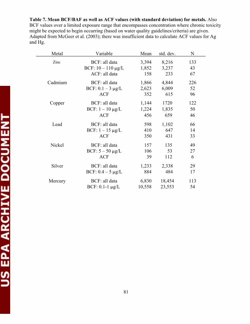
Table 7. Mean BCF/BAF as well as ACF values (with standard deviation) for metals. Also BCF values over a limited exposure range that encompasses concentration where chronic toxicity might be expected to begin occurring (based on water quality guidelines/criteria) are given. Adapted from McGeer et al. (2003); there was insufficient data to calculate ACF values for Ag and Hg.

Metal

Zinc

Cadmium

Copper

Lead

Nickel

Silver

Mercury

Variable

BCF: all dataBCF: 10 – 110 :g/L

ACF: all data

BCF: all dataBCF: 0.1 – 3 :g/L

ACF


ACF


ACF


ACF

BCF: all dataBCF: 0.4 – 5 :g/L

BCF: all dataBCF: 0.1-1 :g/L

Mean std. dev. N

3,394 8,216 133 1,852 3,237 43

158 233 67

1,866 4,844 226 2,623 6,009 52

352 615 96

1,144 1720 122 1,224 1,835 50

456 659 46

598 1,102 66 410 647 14 350 431 33

157 135 49 106 53 27

39 112 6

1,233 2,338 29 884 484 17

6,830 18,454 113 10,558 23,553 54

81

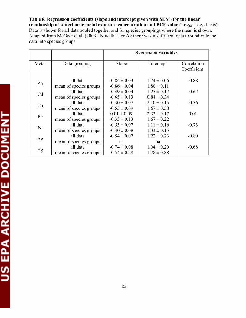
Table 8. Regression coefficients (slope and intercept given with SEM) for the linear relationship of waterborne metal exposure concentration and BCF value (Log10: Log10 basis). Data is shown for all data pooled together and for species groupings where the mean is shown. Adapted from McGeer et al. (2003). Note that for Ag there was insufficient data to subdivide the data into species groups.

Metal

Zn

Cd

Cu

Pb

Ni

Ag

Hg

Regression variables

Data grouping Slope Intercept Correlation Coefficient

all data -0.84 ± 0.03 1.74 ± 0.06 -0.88 mean of species groups -0.86 ± 0.04 1.80 ± 0.11



all data 0.01 ± 0.09 2.33 ± 0.17 0.01 mean of species groups -0.35 ± 0.13 1.67 ± 0.22


all data -0.54 ± 0.07 1.22 ± 0.23 -0.80 mean of species groups na na


82

It is important to note that much of the data on dietborne metal effects arise from laboratory studies of diet only exposure or studies of highly contaminated field sites. Assessments of metals should consider the potential for trophic transfer and toxic response in consumers, and those with significant potential should be examined in detail. In the summer of 2002, SETAC sponsored a workshop on the role of dietary exposure in the aquatic ecological risk assessment of metals. The outcomes of this workshop, to be published by SETAC Press, will include detailed information useful for Agency assessments as well as suggestions for regulatory approaches and future research. It should be an invaluable tool for understanding the trophic transfer potential of metals in aquatic systems.

A general approach to account for potential impacts arising from trophic transfer would be to link bioaccumulation in prey items to exposure in the water column as well as potential impacts in consumers. One methodology to achieve this is to integrate tissue burden to toxicity relationships (prey: predator interactions) with exposure to bioaccumulation relationships (e.g., BCF and BAF values). A theoretical example of this approach, developed by Brix et al. (www.epa.gov/ncea/raf/pdfs/metals/sumryrprt_metals.pdf) is shown in Figure 6. Within the context of this approach, it would be necessary for relevance to ensure that the species being considered were linked within trophic foodwebs (i.e., the exposure to bioaccumulation relationship was for prey items being consumed by the predators that are sensitive to trophic transfer).

Some data already exists to begin these evaluations. For example, it is possible to derive the water concentrations necessary to produce impacts via dietary exposure (see Brix et al. reference above) and site-specific case studies would be valuable in illustrating, testing, and validating these relationships. The potential benefits from this approach would be reducing the uncertainty from extrapolations across exposure concentrations currently being made with metals BCF/BAF data. Also, there would be an ability to link impacts through to waterborne metal concentrations. However, particularly if BCF and BAF data is used, this approach would bring with it the inherent uncertainty associated with predicting tissue metals burdens (e.g., the high variability) and the inability to account for geochemical influences on uptake and accumulation.

Alternatives to Tissue Burdens and Bioaccumulation. One of the key parameters that a bioaccumulation measure should be validated against is chronic toxicity. Since the use of bioaccumulation criteria within the context of PBT is used as a indicator of chronic toxicity (Franke et al., 1994; OECD 2001), validation of linkages to chronic metal toxicity would provide confidence in their use and application. A number of key issues should be addressed when considering bioaccumulation of metals in relation to the potential for chronic impacts, and these add uncertainty to the interpretation of data. However, unlike the substances that the PBT concept was originally developed for, there is often substantial information on the chronic toxicity of metals.

83

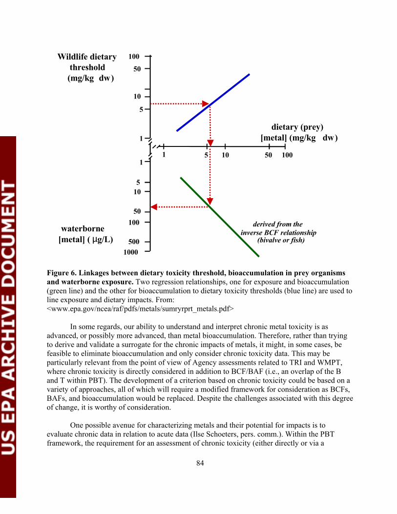
Wildlife dietary threshold (mg/kg dw)

waterborne [metal] ( µg/L)

100

50

10

5

dietary (prey) 1 [metal] (mg/kg dw)

100 1

5 10

50 100 derived from the

inverse BCF relationship 500 (bivalve or fish)

1 5 0 50 1

1000

Figure 6. Linkages between dietary toxicity threshold, bioaccumulation in prey organisms and waterborne exposure. Two regression relationships, one for exposure and bioaccumulation (green line) and the other for bioaccumulation to dietary toxicity thresholds (blue line) are used to line exposure and dietary impacts. From: <www.epa.gov/ncea/raf/pdfs/metals/sumryrprt_metals.pdf>

In some regards, our ability to understand and interpret chronic metal toxicity is as advanced, or possibly more advanced, than metal bioaccumulation. Therefore, rather than trying to derive and validate a surrogate for the chronic impacts of metals, it might, in some cases, be feasible to eliminate bioaccumulation and only consider chronic toxicity data. This may be particularly relevant from the point of view of Agency assessments related to TRI and WMPT, where chronic toxicity is directly considered in addition to BCF/BAF (i.e., an overlap of the B and T within PBT). The development of a criterion based on chronic toxicity could be based on a variety of approaches, all of which will require a modified framework for consideration as BCFs, BAFs, and bioaccumulation would be replaced. Despite the challenges associated with this degree of change, it is worthy of consideration.

One possible avenue for characterizing metals and their potential for impacts is to evaluate chronic data in relation to acute data (Ilse Schoeters, pers. comm.). Within the PBT framework, the requirement for an assessment of chronic toxicity (either directly or via a

84

surrogate measure such as bioaccumulation) depends in part on how well acute toxicity captures the potential for impacts. For metals with a low acute to chronic ratio (ACR), addressing chronic toxicity will not add significantly to the assessment because it will duplicate the concern that acute toxicity captures. However, for metals with a high ACR it would be relevant and important to assess the potential for chronic impacts. As in the case of dietary toxicity, this method will serve as a screening tool to identify metals that might warrant further detailed examination. For example the ratio of CMC to CCC criteria values for Zn (1) or Cu (1.4) compared to that for Pb (26) might suggest that the latter should receive more focused effort in terms of assessing chronic impacts and/or bioaccumulation. In practice, the application of this approach may be problematic as ACR data are quite variable across species and are fraught with problems such as those related to chronic test duration and the testing of the life stage.

The conceptual model of Rainbow (1999; 2002; see section 4.2.2), the essence of which is a modified spillover hypothesis model, may be useful for considering bioaccumulation in relation to toxicity. The increase of metabolically available bioaccumulated metal, and whether the toxicity threshold concentration is reached depends on the rate of metal uptake relative to the rate of removal from the pool via elimination and storage. The key variables in this model relate to the rates up uptake, elimination, and storage. If the rate of uptake exceeds the combined rates of elimination and storage, then the metal level in the metabolic pool will increase eventually resulting in effects. The application of this conceptual model requires a significant understanding of accumulation from both waterborne and dietary sources, as well as the physiological processes involved in uptake, internal handling, storage, and elimination of metals. Because our level of understanding is currently lacking, we encourage research that will help to deliver the data required to build the database necessary to establish this type of assessment process. As research develops it may be possible to initially consider these approaches on a site-specific basis, followed by more general applications with increased understanding.

Emerging Techniques for Addressing Bioavailability and Bioaccumulation. Of the many issues related to bioavailability, one that is often overlooked is the transformation and dissolution of metal substances. Assessments and evaluations for aquatic systems are primarily done on the basis of dissolved metal concentration but many metals are used as insoluble or sparingly soluble substances. Previous approaches which assume that all substances have the potential to produce dissolved metal species have recently been refined to account for the rate of transformation and dissolution into aquatic media. This approach, which has been developed through the OECD’s globally harmonized system for hazard classification, links the rate and extent of chemical dissolution with the relative toxicity of the metal being released. Although these concepts might not be directly applicable to processes conducted by the Agency, they may be of value in helping to focus on accounting for the fraction of metal that is bioavailable in aquatic systems.

Similarly, while this issue paper does not deal with the issue of persistence, it is useful to note that one of the proposed solutions for the issue of persistence, such as assessing the half-life of dissolved metal species in the water column (Skeaff et al., 2002), can be refined through linkages to bioavailability as the persistence of bioavailable forms is of greatest concern.

Mechanistic approaches for assessing and predicting metal bioavailability, bioaccumulation, and toxicity hold substantial promise compared to purely empirical methods,

85

and they need continued research support. Specifically, expansion of BLM models to address acute toxicity, dietary uptake (for those metal-receptor scenarios where this is of particular concern), and chronic toxicity is strongly encouraged, and some work in this regard is ongoing. Linkage of BLM-type approaches to pharmacokinetic models may be needed for some metals since data indicate that the kinetics of metal bioaccumulation can govern the expression of effects, not just the extent of bioaccumulation and partitioning of metals.

In situations where trophic transfer is of concern, research to quantify the fraction of metal in tissues that is most bioavailable to aquatic and terrestrial consumers should be conducted, keeping in mind the effects of food preparation (cooking) on bioavailability to human consumers. Available kinetic models for predicting metal bioaccumulation in aquatic food webs show the most promise when applied and calibrated on a site-specific basis, and efforts should continue to refine, evaluate, and apply these models where more intensive efforts are warranted. For these steps to refine predictions of metal bioavailability and bioaccumulation to be successful, greater understanding of the mechanistic basis of metal toxicity will be needed to define the output requirements of bioaccumulation models. A simple but important role that the Agency (and others) can have in promoting these approaches is to ensure that the data on metals that is collected is sufficient and complete enough to support current and future attempts to integrate data into the developing models.

BLM approaches are continuing to be developed for both acute and chronic metal toxicity, although the latter are certainly less developed. In the case of acute toxicity, the original mechanistic derivation of the relationship between geochemistry and toxic bioaccumulation in the fish gill appears to be sufficiently robust to permit the successful extension to a variety of species and model calibration solely to toxicity. However for chronic toxicity predictions there is a need to further refine these geochemistry, bioaccumulation, and toxicity relationships. One of the difficulties in developing chronic toxicity prediction models relates to a the lack of knowledge on chronic toxicity endpoint, particularly from the point of view of bioaccumulated metals.

Research on chronic BLMs is continuing and has met with some success. For example chronic BLMs for Zn have been developed for three trophic levels (algae, invertebrates, fish), and their application has recently been proposed in the context of the Zn risk assessment exercise that is being conducted within the European Union (H. Waeterschoot, pers comm.). Chronic Cu BLMs are also being developed for a similar EU risk assessment for Cu. The proposed application of the newly developed chronic BLMs for Zn is as exposure geochemistry specific modifiers of baseline criteria values. This application is essentially using the model as a water effect ratio (WER) adjustment tool, which was one of the original suggested applications of the acute BLMs (Di Toro et al., 2001). Using chronic BLMs in this manner would serve to integrate site-specific considerations into assessments at a variety of different levels. Studies are currently underway to apply this WER approach to assessing the potential for chronic impacts downstream of mine effluent discharges. In the case of Cu and Ag, the use of BLM approaches would appear to offer significant advantages over hardness adjustments in accounting for site specific geochemistry effects on toxicity (B. Vigneault and M. Schwartz pers. comm.).

The future developments of BLM approaches will revolve around improved understanding of metal uptake and distribution in biota, which has been discussed by Paquin et al. (2002) and more broadly in the September 2002 special issue of Comparative Biochemistry and

86

Physiology Part C. It would seem likely that the development of modeling approaches for chronic bioaccumulation and toxicity may require alternative approaches to those of the acute BLM which relies on equilibrium modeling. For example, a physiologically-based model with internal Na+ balance as the modeling endpoint has been proposed by Paquin et al. (2002). Other physiologically-based models are proposed for development, which account for aquatic geochemistry in terms of uptake from multiple exposure surfaces (gill, GI tract), exchange within body compartments, detoxification, and elimination. These will likely serve to integrate and apply existing, ongoing, and future research results.

5.2 Research Needs

5.2.1 Aquatic

Future areas of research to better understand bioaccumulation processes involving metals in aquatic organisms include:

• Evaluation of the bioaccumulation of metals bound to colloidal material in ambient water.

• More thorough evaluation of the efflux rates of metals from different animals, including specific tissues, following bioaccumulation from the dissolved phase and from the dietary pathway.

• Evaluation of metal bioaccumulation in aquatic bacteria, which may influence the fluxes of certain metals in aquatic systems and which may introduce metals into bacteria-based food chains.

• For organisms that are used or at least have the potential to serve as bioindicator organisms, a more detailed knowledge base is required on their basic physiology and ecology; further, monitoring programs could focus on key biomarkers of exposure and effects and would be wise to develop an algorithm to calculate an integrated stress index.

• New approaches to evaluate the bioaccumulation of metals from waters in which there are numerous contaminants (such as would be found in most contaminated harbors or rivers) to assess synergistic and antagonistic effects.

5.2.2 Terrestrial

Soil organisms. Future areas of research to better understand bioavailability and bioaccumulation involving metals and soil-dwelling organisms include:

• Development and validation of empirical and mechanistic models linking soil physicochemical characteristics, metal speciation, and toxic effects and bioaccumulation in soil invertebrates (e.g., BLM for soil organisms).

• Development and validation of kinetics models describing metal bioaccumulation in soil invertebrates.

87

• Basic research on the physiology of metal metabolism in various groups of soil invertebrates; evaluation of the relevance of soil pore water or diet in exposure and partitioning of metals in soil invertebrates.

• Identification of the risks for predators associated with the consumption of soil invertebrates containing metals; evaluation of the risk of consumption of by predators of metal partitioned to different fractions in soil invertebrates (e.g., storage granules versus metallothionein).

• Development of metal-specific biomarkers capable of quantitatively detecting magnitude and species of metal exposure.

6. LITERATURE CITED

Adams, W.J. 2000. Hazard identification for metals and metal compounds: An alternative to the U.S. EPA strategy for identifying hazards associated with metals and metal substances. Presentation at the expert workshop: state of the science regarding PBT concepts and metals and metal compounds. U.S. EPA, EPRI, ICA, ILZRO, NiPERA and ICME. Arlington, VA. January 19.

Adams, P.C., R. Zhong, J. Haist, P.R. Flangan and D.R. Grant. 1991. Mucosal iron in the control of iron absorption in rat intestinal transplant model. Gastroenterology, 100: 370-374.

Alsop, D.K. and C.M. Wood. 2000. Kinetic analysis of zinc accumulation on the gills of juvenile rainbow trout: effects of zinc acclimation and implications for biotic ligand modeling. Environ. Toxicol. Chem. 19:1911-1918.

Alsop, D.K., J.C. McGeer, D.G. McDonald and C.M. Wood. 1999a. Costs of chronic waterborne zinc exposure and the consequences of zinc accumulation on the gill/zinc interactions of rainbow trout in hard and soft water. Environ. Toxicol. Chem. 18:1014-1025.

Alsop, D.H., J.C. McGeer, D.G. McDonald and C.M. Wood. 1999b Assessing the costs and consequences of chronic waterborne zinc exposure to juvenile rainbow trout in hard and soft water. Environ. Toxicol. Chem. 18: 1014-1025.

Angle, C.R., A. Marcus, I.-H. Chengand M.S. and McIntire. 1984. Omaha childhood blood lead and environmental lead: A linear total exposure model. Environ. Res. 35:160-170.

Ankley, G.T., N.A. Thomas, D.M. Di Toro, D.J. Hansen, J.D. Mahony, W.J. Berry, R.C. Swartzand and R.A. Hoke. 1994. Assessing potential bioavailability of metals in sediments: A proposed approach. Environ. Manage. 18:331-337.

Archer, D., S. Emersonand and C. Reimers. 1989. Dissolution of calcite in deep-sea sediments: pH and oxygen microelectrode results. Geochim. Cosmochim. Acta 53:2831-2845.

American Society of Testing and Materials (ASTM). 1997. Standard guide for determination of bioaccumulation of sediment-associated contaminants by benthic invertebrates. E1688-97a. In: ASTM annual book of standards, v. 11.05. American Society of Testing and Materials, Philadelphia, PA, pp. 1072-1121.

88

Baines, S.B., N.S. Fisher and R. Stewart. 2002. Assimilation and retention of selenium and other trace elements from crustacean food by juvenile striped bass (Morone saxatilis). Limnol. Oceanogr. 47:646-655.

Banerjee, S., S.H. Yalkowsky, and S.C. Valvani. 1980. Water solubility and octanol/water partition coefficients or organics. Limitations of the solubility-partition coefficient correlation. Environ. Sci. Technol. 14: 1227-1229.

Barltrop, D. 1973. Sources and significance of environmental lead for children. In: Proceedings of the International Symposium on Environmental Health Aspects of Lead. Commission of European Communities, Center for Information and Documentation, Luxemburg.

Barltrop, D. and F. Meek. 1979. Effect of particle size on lead absorption from the gut. Arch. Environ. Health 34:280-285.

Barron, M.G. 1990. Bioconcentration. Environ. Sci. Technol.1612-1618.

Barron, M.G., G.R. Stehly, and W.L. Hayton. 1990. Pharmacokinetic modeling in aquatic animals I. models and concepts. Aquat. Toxicol. 18: 61-86.

Basta, N.T., D.J. Pantone and M.A. Tabatabai. 1993. Path analysis of heavy metal adsorption by soil. Agron. J. 85:1054-1057.

Beckett, P.H.T. 1989. The use of extractants in studies on trace metals in soil, sewage sludges, and sludge-treated soils. Adv. Soil Sci. 9:143-176.

Belfroid, A., M. Van der Berg, W. Seinen, J. Hermens and C.A.M. Van Gestel. 1995. Uptake, bioavailability and elimination of hydrophobic compounds in earthworms (Eisenia andrei) in field-contaminated soil. Environ. Toxicol. Chem. 14:605-612.

Benet, L.Z., Kroetz, D.L. and L.B. Sheiner. 1996. Pharmacokinetics: The dynamics of drug absorption, distribution, and elimination. In: Molinoff, P.B., and R.W. Ruddon, eds. Goodman and Gilman’s The pharmacological basis of therapeutics. New York: McGraw Hill.

Berger, B., R. Dallinger and A. Thomaser. 1995. Quantification of metallothionein as a biomarker for cadmium exposure in terrestrial gastropods. Environ. Toxicol. Chem. 14:781-791.

Bergman, H.L. and E.J. Doward-King. 1997. Reassessment of metals criteria for aquatic life protection. SETAC Press, Pensacola, FL.

Berry, W.J., M. Cantwell, P. Edwards, J. Serbst and D.J. Hansen. 1999. Predicting the toxicity of sediments spiked with silver in the laboratory. Environ. Toxicol. Chem. 18:40-48.

Bezwoda, W., R. Charlton, T. Bothwell, J. Torrance and F. Mayet, 1978. The importance of gastric hydrochloric acid in the adsorption of nonheme food iron. J. Lab. Clin. Med. 41:108-116.

Bingham, F.T., G. Sposito, and J.E. Strong. 1986. The effect of sulfate on the availability of cadmium. Soil Sci. 141:172-177.

89

Bjerregaard, P., S. Topçuo_lu, N.S. Fisher and S.W. Fowler. 1985. Accumulation and retention of 237Pu and 241Am in the mussel Mytilus edulis. Mar. Ecol. Prog. Ser. 21:99-111.

Bleeker, E.A.J., M.H.S. Kraak and C. Davids. 1992. Ecotoxicity of lead to the zebra mussel Dreissena polymorpha, Pallas. Hydrobiol. Bull. 25:233-236.

Bodar, C.W.M., I. van der Sluis, J.C.P. van Montfort, P.A. Voogt and D.I. Zandee. 1990. Cadmium resistance in Daphnia magna. Aquat. Toxicol. 16:33-40

Bornschein, R.L., Succop, P.A., Krafft, K.M., Clark, C.S., et al. 1987. Exterior surface dust lead, interior house dust lead and childhood lead exposure in an urban environment. In: Hemphill, D.D. (Ed.), Trace Substances in Environmental Health–XX. Proceedings of the University of Missouri’s 20th annual Conference, June 1986, pp. 322-332. University of Missouri, Columbia, MO.

Bradham, K.D. 2002. Effect of soil properties on the bioavailability and toxicity of metals to Eisenia andrei. Ph.D. diss, Dept. of Zoology, Oklahoma State University.

Bradley, R.W., C. DuQuesnay and J.B. Sprague. 1985. Acclimation of rainbow trout, Salmo gairdneri Richardson, to zinc: Kinetics and mechanism of enhanced tolerance induction. J. Fish Biol. 27: 367-379.

Branson, D.R., G.E. Blau,, H.C. Alexander, and W.B. Neely. 1975. Bioconcentration of 2,2’,4,4’-tetrachlorobiphenyl in rainbow trout as measured by an accelerated test. Trans. Am . Fish. Soc. 4:785-792.

Brix, K.V. and D.K. DeForest. 2000. Critical review of the use of bioconcentration factors for hazard classification of metals and metal compounds. Parametrix, Inc., Kirkland, WA. April. 71+pp.

Brown, B.E. 1982. The form and function of metal-containing 'granules' in invertebrate tissues. Biol. Rev. 57:621-667.

Brown, S.L., C.L. Henry, H. Compton, R.L. Chaney, and P. DeVolder. 2000. Using municipal biosolids in combination with other residuals to restore metal-contaminated mining areas. Chap. 1 in: Proceedings of a Symposium on Mining, Forest and Land Restoration: The Successful Use of Residual/Biosolids/Organic Matter for Reclamation Activities. Denver, CO.: Rocky Mountain Water Environment Association. July 17-20.

Brown, S.L., R.L. Chaney, and W. Berti. 1999. Field test of amendments to reduce the insitu availability of soil lead. In: Abstracts of the 5th International Conference on Biogeochemistry of Trace Elements. Wenzel, W.w., D.C. Adriano, B. Alloway, H.E. Dorner, C. Keller, N.W. Lepp, M. Mench, R. Naidu, and G.M. Pierzynski, eds. Vienna, Austria: International Society for Trace Element Research. July 11-15, pp. 506-507.

90

Brown, L., S. Casteel, R. Cowart, J. Turk, T. May, E. Hoffman, G. Henningsen, C. Weis and W. Brattin. 1998. Composite soil lead relative bioavailability in three age categories of swine. Toxicologist 127, p. 25.

Brown, L., R. Cowart, J. Turk, T. May, E. Hoffman, G. Henningsen, C. Weis and S. Casteel. 1998. Key advantages of swine gestational and transplacental model for metal bioavailability. Toxicol. Lett. 95(Suppl. 1):215.

Brunekreef, B.D., D. Noy, K. Biersteker and J. Boleij. 1983. Blood-lead levels of Dutch city children and their relationship to lrad in the environment. J. Air Pollut. Control Assoc. 33:872-876.

Bustamante, P., F. Caurant, S.W. Fowler and P. Miramand. 1998. Cephalopods as a vector for the transfer of cadmium to top marine predators in the north-east Atlantic Ocean. Sci. Total. Environ. 220:71-80.

Calabrese, E.J., P.T. Kosteecki and C.E. Gilbert. 1987. How much soil do children eat? An emerging consideration for environmental health risk assessment. Comments Toxicol.

Calamari, D., G.F. Gaggino, and G. Pacchetti. 1982. Toxicokinetics of low levels of Cd, Cr, Ni and their mixture in long-term treatment on Salmo gairdneri Rich. Chemosphere 11: 59-70.

Campbell, P.G.C. 1995. Interactions between trace metals and aquatic organisms: A critique of the free-ion activity model. In: Tessier, A. and D.R. Turner, eds. Metal Speciation and Bioavailability in Aquatic Systems. Chichester, UK: Wiley, pp. 45-102.

Casteel, S., L. Brown, R. Cowart, J. Turk, T. May, E. Hoffman, G. Henningsen, C. Weis and W. Brattin. 1998. Lead disposition in maternal and fetal swine tissues. Toxicologist 1062, p. 216.

Casteel, S., L. Brown, R. Cowart, L. Pace, C. Weis, E. Hoffman and G. Henningsen. 1998. Bioavailability of arsenic in contaminated media. Toxicol. Lett. 95(Suppl. 1):135.

Casteel, S., L. Brown, R. Cowart, J. Turk, T. May, E. Hoffman, G. Henningsen and C. Weis. 1998. Distribution of lead in the pregnant swine model. Toxicol. Lett. 95(Suppl. 1):127.

Casteel, S.W., R.P. Cowart, J.T. Payne, S.L. Stockman, J.R. Turk, C.P. Weis, G.M. Henningsen, E. Hoffman, W.J. Brattin and S.V. Becker. 1996. Determining the bioavailability of lead in contaminated soil. Toxicologist 30(1, pt. 2):11.

Casteel, S., R. Cowart, C. Weis, G. Henningsen, E. Hoffman, W. Brattin, R. Guzman, M. Starost, J. Payne, S. Stockham, S. Becker, J. Drexler and J. Turk. 1997. Bioavailability of lead to juvenile swine dosed with soil from the Smuggler Mountain NPL Site of Aspen, Colorado. Fund Appl Toxicol. 36:177-187.

Casteel, S.W., Cowart, R.P., Weiss, C.P., Henningsen, G.M.,Hoffman, E., Brattin, W.J., Guzman, R.E., Starost, M.F., Payne, J., Stockman, S.L., Becker, S.V., Drexler, J.W. and Turk, J.R., 1997. Bioavailability of Lead in Soil from the Smuggler Mountain Site of Aspen, Colorado. Fundam. Appl. Toxicol. 36:177-187.

91

CB Research International. 1993. Report: Development of a physiologically relevant extraction procedure. Sidney, BC, Canada, 68 pp.

Chaney, R.L. and J.A. Ryan. 1994. Risk-based standards for arsenic, lead and cadmium in urban soils. Frankfurt, Germany: DECHMEA.

Chaney, R.L., S.L. Brown, J.S. Angle, T.I. Stuczynski, W.L. Daniels, C.L. Henry, G. Siebielec, Y.M. Li, J.A. Ryan and H. Compton. 2000. In situ remediation/reclamation/restoration of metals contaminated soils using tailor-made biosolids mixtures. In: Proceedings of Mining, Forest and Land Restoration Symposium/Workshop. Rocky Mountain Water Environment Association Biosolids Committee. July 17-19, Golden, CO.

Chang, S.I. and J.R. Reinfelder. 2000. Bioaccumulation, subcellular distribution, and trophic transfer of copper in a coastal marine diatom. Environ. Sci. Technol. 34:4931-4935.

Chang, A.C., A.L. Page, and J.E. Warneke. 1984. A sequential extraction of soil heavy metals following sludge application. J. Environ. Qual. 13:33-38.

Chapman, P.M. 1996. Hazard identification, hazard classification and risk assessment for metals and metal compounds in the aquatic environment. International Council on Metals and the Envrionment. Ottawa, Canada. 31 pp.

Chapman, P.M., H.E. Allen, K. Godtfredsen and M.N. Z'Graggen. 1996. Evaluation of bioaccumulation factors in regulating metals. Environ. Sci. Technol. 30:448-452.

Charlatchka, R., P. Cambier and S. Bourgeois. 1997. Mobilization of trace metals in contaminated soils under anaerobic conditions. In: Prost, R. ed. Contaminated soils, Proceedings of the 3rd International Conference on Biogeochemistry Trace Elements, Paris (France). May 15-19. pp. 159-174.

Chen, Z. and L.M. Mayer. 1999. Sedimentary metal bioavailability determined by the digestive constraints of marine deposit feeders: gut retention time and dissolved amino acids. Mar. Ecol. Prog. Ser. 176:139-151.

Chiou, C.T., V.H. Freed, D.W. Schmedding and R.L. Kohnert. 1977. Partition coefficient and bioaccumulation of selected organic chemicals. Environ. Sci. Tech. 11: 475-478

Clayton Jr., J.R., S.P. Pavlou and N.F. Beitner. 1977. Polychlorinated biphenyls in coastal marine zooplankton: Bioaccumulation by equilibrium partitioning. Environ. Sci. Technol. 11: 676-682

Conder, J.M., L.D. Seals and R.P. Lanno. 2002. Method for determining toxicologically relevant cadmium residues in the earthworm Eisenia fetida. Chemosphere 49:1-7.

Cowart, R., L Brown, S. Casteel, J. Turk, T. May, E. Hoffman, G. Henningsen, C. Weis, W. Brattin and T. Hammon. 1998. A mathematical formula for characterizing maternal contributions to fetal tissue lead. Toxicologist 1063:216. Seattle, WA, Mar 1-5.

92

Cowgill, U.M. 1976. The chemical composition of two species of Daphnia their algal food and their environment. Sci. Total Environ. 6: 79-102.

Crommentuijn, T., C.J.A.M. Doodeman, J.J.C. Van der Pol, A. Doornekamp, M.C.J. Rademaker and C.A.M. Van Gestel. 1994. Lethal body concentrations and accumulation patterns determine time-dependent toxicity of cadmium in soil arthropods. Environ. Toxicol. Chem. 13:1781-1789.

Crommentuijn, T., C.J.A.M. Doodeman, J.J.C. Van der Pol, A. Doornekamp and C.A.M. Van Gestel. 1997. Bioavailability and ecological effects of cadmium on Folsomia candida (Willem) in an artificial soil substrate as influenced by pH and organic matter. Appl. Soil Ecol. 5:261-271.

Dahlgaard, H. 1986. Effects of season and temperature on long-term in situ loss rates of Pu, Am, Np, Eu, Ce, Ag, Tc, Zn, Co and Mn in a Baltic Mytilus edulis population. Mar. Ecol. Prog. Ser. 33:157-165.

Dallinger, R. 1996. Metallothionein research in terrestrial invertebrates: Synopsis and perspectives. Comp. Biochem. Physiol. 113C:125-133.

Dallinger, R., B. Berger, P.E. Hunziker and J.H.R. Kagi.1997. Metallothionein in snail Cd and Cu metabolism. Nature 388:237-238.

Davidson, W., G.W. Grime, J.A.W. Morgan and K. Clarke. 1991. Distribution of dissolved iron in sediment pore waters at submillimetre resolution. Nature 352:323-325.

Davidson, W. and H. Zhang. 1994. In situ speciation measurements of trace components in natural waters using thin-film gels. Nature 367:546-548.

Davidson, W. and H. Zhang and G.W. Grime. 1994. Performance characteristics of gel probes used for measuring pore waters. Environ. Sci. Technol. 28:1623-1632.

Davis, A., J.W. Drexler, M.V. Ruby and A. Nicholson. 1993. Micromineralogy of mine wastes in relation to lead bioavailability, Butte, Montana. Environ. Sci. Technol. 27:1415-1424.

de Nicola, M., N. Cardellicchio, C. Gambardella, S.M. Guarino and C. Marra. 1993. Effects of cadmium on survival, bioaccumulation, histopathology and PGM polymorphism in the marine isopod Idotea baltica, In Ecotoxicology of Metals in Invertebrates, Dallinger R, Rainbow PS, eds. Boca Raton, FL: Lewis Publishers, pp 103-116.

de Schamphelaere, K.A.C., D.G. Heijerick and C.R. Janssen. 2002. Refinement and field validation of a biotic ligand model predicting acute copper toxicity to Daphnia magna. Comp. Biochem. Physiol. 133C: 243-258.

Devillers, J. D. Domine, S. Bintein and W. Karcher. 1998. Comparison of fish bioconcentration models. In: Comparative QSAR. Devillers, J, ed.. Washington D.C.: Taylor and Francis, pp. 1-50.

Di Toro, D.M., H.E. Allen, H.L. Bergman, J.S. Meyer, P.R. Paquin and R.C. Santore. 2001. Biotic ligand model of the acute toxicity of metals. 1. Technical basis. Environ. Toxicol. Chem. 20:2383-2396.

93

Di Toro, D.M., D.J. Hansen, J.A. McGrath and W.J. Berry. 1999. Predicting the toxicity of metals in sediments. Integrated approach to assessing the bioavailability and toxicity of metals in surface waters and sediments. USEPA 822-E-99-01.

Di Toro, D.M., J.D. Mahony, D.J. Hansen, K.J. Scott, A.R. Carlson and G.T Ankley. 1992. Acid volatile sulfide predicts the acute toxicity of cadmium and nickel in sediments. Environ. Sci. Technol. 26:96-101.

Di Toro, D.M., J.D. Mahony, D.J. Hansen, K.J. Scott, M.B. Hicks, S.M. Mayr and M.S. Redmond. 1990. Toxicity of cadmium in sediments: The role of acid volatile sulfide. Environ. Toxicol. Chem. 9:1487-1502.

Drexler, J.W. 1997. Validation of an in vitro method: A tandem approach to estimating the bioavailability of lead and arsenic in humans. Presented at IBC Conference on Bioavailability, Scottsdale, AZ.

Drexler, J.W. and P. Mushak.1995. Health risks from extractive industry wastes: Characterization of heavy metal contaminants and quantification of their bioavailability and bioaccessibility. In: Prost, R. ed. Contaminated soils. Proceedings of the 3rd International Conference on Biogeochemistry Trace Elements, Paris (France). May 15-19.

Drexler, J.W., C. Weis and W. Brattin. 2003. Relative bioavailability of lead: A validated in vitro procedure. J. Appl. Toxicol. Submitted.

Endo, T., S. Nakaya, R. Kimura and T. Murata. 1986. Gastrointestinal adsorption of inorganic mercuric compounds in vitro. Toxicol. Appl. Pharmacol. 83:187-196.

Erickson, R.J. and J.M. McKim. 1990. A model for exchange of organic chemicals at fish gills: flow and diffusion limitations. Aquat. Toxicol. 18: 175-198.

Erickson, R.J., D.A. Benoit, V.R. Mattson, H.P. Nelson Jr. and E.N. Leonard. 1996. The effects of water chemistry on the toxicity of copper to fathead minnows. Environ. Toxicol. Chem. 15: 181-193.

Everett, S., G. Henningsen, M. Wickstrom, R. Graham, S. Callio, P. Mushovic, B. Everett and D. Bird. 1998. Tissue concentrations of selected metals and radionuclides in exposed cattle, deer and other biota near a former uranium mill processing site. Toxicologist 1134.

Federal Register, 1989, Final Rule for Good Laboratory Practice Standards Under the Federal Insecticide, Fungicide, and Rodenticide Act, Code of Federal Regulations Title 40, Pt. 160; pp. 34067-34074.

Feijtel, T., P. Kloepper-Sams, K. den Haan, R. van Egmond, M. Comber, R. Heusel, P. Wierich, W. Ten Berge, A. Gard, W. de Wolf and H. Niessen. 1997. Integration of bioaccumulation in an environment of risk assessment. Chemosphere 34: 2337-2350.

Fisher, N.S. 1985. Accumulation of metals by marine picoplankton. Mar. Biol. 87:137-142.

94

Fisher, N.S., M. Bohé and J.-L. Teyssié. 1984. Accumulation and toxicity of Cd, Zn, Ag, and Hg in four marine phytoplankters. Mar. Ecol. Prog. Ser. 18:201-213.

Fisher, N.S. and M. Wente. 1993. The release of trace elements by dying marine phytoplankton. Deep-Sea Res. 40:671-694.

Fisher, N.S. and J.R. Reinfelder. 1995. The trophic transfer of metals in marine systems. In: Tessier, A. and D.R. Turner, eds. Metal speciation and bioavailability in aquatic systems. Chichester, UK: Wiley, pp. 363-406.

Fisher, N.S., J.-L. Teyssié, S.W. Fowler and W.-X. Wang. 1996. Accumulation and retention of metals in mussels from food and water: a comparison under field and laboratory conditions. Environ. Sci. Technol. 30:3232-3242.

Fisher, N.S., I. Stupakoff, S.A. Sañudo-Wilhelmy, W.-X. Wang, J.-L. Teyssié, S.W. Fowler and J. Crusius. 2000. Trace metals in marine copepods: a field test of a bioaccumulation model coupled to laboratory uptake kinetics data. Mar. Ecol. Prog. Ser. 194:211-218.

Foerstner, U. 1987. Sediment-associated contaminants: An overview of scientific basis for developing remidial options. Hydrobiologia, 149:221-246.

Fowler, S.W. 1982. Biological transfer and transport processes. In: Kullenberg, G., ed. Pollutant transfer and transport in the sea, Vol.II, Boca Raton, FL: CRC Press, pp. 1-65.

Foy, C.D., R.L. Chaney and M.C. White. 1978. The physiology of metal toxicity in plants. Ann. Rev. Plant Physiol. 29:511-566.

Franke, C. 1996. How meaningful is the bioconcentration factor for risk assessment? Chemosphere 32: 1897-1905.

Franke, C., G. Studinger, G. Berger, D. Bohling, U. Bruckmann, D. Cohors-Fresenborg and U. Johncke. 1994. The assessment of bioaccumulation. Chemosphere 29:1501-1514.

Freeman, G.B., J.D. Johnson, J.M. Killinger, S.C. Liao, A.O. Davis, M.V. Ruby, R.L. Chaney, S.C. Lovre and P.D. Bergstrom. 1993. Bioavailability of arsenic in soil impacted by smelter activities following oral administration in rabbits. Fund. Appl. Toxicol. 21: 83-88.

Gagnon, C. and N.S. Fisher. 1997. The bioavailability of sediment-bound Cd, Co, and Ag to the mussel Mytilus edulis. Can. J. Fish. Aq. Sci. 54:147-156.

Gasser, U.G., W.J. Walker, R.S. Borch and R.G. Burau. 1996. Lead release from smelter and mine waste impacted materials under simulated gastric conditions and relation to speciation. Environ. Sci. Technol. 30:761-769.

George, S.G., B.J.S. Pirie, A.R. Cheyne, T.L. Combs and P.T. Grant. 1978. Detoxification of metals by marine bivalves; ultrastructural study of the compartmentalisation of copper and zinc in the oyster, Ostrea edulis. Mar. Biol. 45:147-156.

95

George, S.G. and B.J.S. Pirie. 1980. Metabolism of zinc in the mussel, Mytilus edulis (L.): A combined ultrastructural and biochemical study. J. Mar. Biol. Assoc. U.K. 60:575-590.

George, S.G. 1990. Biochemical and cytological assessments of metal toxicity in marine animals. In: Heavy metals in the marine environment. Furness, R.W. and P.S. Rainbow, eds. Boca Raton, FL: CRC Press, pp.123-142.

Gettier, S.W., D.C. Martens and S.I. Donohue. 1985. Soybean yield response prediction from soil and tissue manganese levels. Agron. J. 77:63-67.

Goldberg, E.D., V.T. Bowen, J.W. Farrington, G.R. Harvey, J.H. Martin, P.L. Parker, R.W. Risebrough, W. Robertson, E. Schneider and E. Gamble. 1978. The mussel watch. Environ. Cons. 5:101-125.

Goldberg, E.D., M. Koide, V. Hodge, A.R. Flegal and J. Martin. 1983. US Mussel Watch: 1977-1978. Results on trace metals and radionuclides. Estuar. Coastal Shelf Sci. 16:69-93.

Gorree, M., W.L.M. Tamis, T.P. Traas and M.A. Elbers. 1995. BIOMAG: A model for biomagnification in terrestrial food chains. The case of cadmium in the Kempen, The Netherlands. Sci. Total Environ. 168:215-223.

Gray, J.S., 2002. Biomagnification in marine systems: the perspective of an ecologist. Mar. Pollut. Bull. 45:46-52.

Griffin, S., C. Weis and A. Marcus.1993. Application of a pharmacokinetic model in assessing risk to multi-media lead exposure at the Butte, Montana, Superfund site. Toxicologist 13:142.

Griscom, S.B., N.S. Fisher and S.N. Luoma. 2002. Kinetic modeling of Ag, Cd and Co bioaccumulation in the clam Macoma balthica; quantifying dietary and dissolved sources. Mar. Ecol. Prog. Ser. 240:127-141.

Grosell, M.H., C. Hogstrand and C.M. Wood. 1997. Cu uptake and turnover in both Cu-acclimated and non-acclimated rainbow trout (Oncorhynchus mykiss). Aquat. Toxicol. 38:257-276.

Grosell, M.H., J.C. McGeer and C.M. Wood. 1998. Renal Cu and Na excretion and hepatic Cu metabolism in both Cu-acclimated and non-acclimated rainbow trout (Oncorhynchus mykiss). Aquat. Toxicol. 40:275-291.

Grosell, M.H., C. Hogstrand and C.M. Wood. 2001. Copper toxicokinetics and hepatobiliary excretion in copper-acclimated and non-acclimated freshwater rainbow trout (Oncorhynchus mykiss). Am. J. Physiol. 280:797-806.

Gundersen, J.K., E.L. Jorgensen, E. Larsen and H.W. Jannasch. 1992. Mats of giant sulfur bacteria on deep-sea sediments due to fluctuating hydrothermal flow. Nature 360:454-455.

Gupta, S.K. and K.Y. Chen. 1975. Partitioning of trace elements in selective chemical fractions of nearshore sediments. Environ. Lett. 10:129-158.

96

Hamilton, S.J. and P.M. Mehrle. 1986. Metallothionein in fish: review of its importance in assessing stress from metal contaminants. Trans. Am. Fish. Soc. 115:569-609.

Handy, R.D. 1993. The effect of acute exposure to dietary Cd and Cu on organ toxicant concentrations in rainbow trout, Oncorhynchus mykiss. Aquat. Toxicol. 27:1-14.

Hansen, D.J., W.J. Berry, J.D. Mahony, W.S. Boothman, D.L. Robson and G.T. Ankley. 1996. Predicting the toxicity of metals-contaminated field sediments using interstitial concentration of metal and acid volatile sulfide normalizations. Environ. Toxicol. Chem. 15:2080-2094.

Harris, Z.L. and J.D. Gitlin. 1996. Generic and molecular basis for copper toxicity. Am. J. Clin. Nutr. 63: 836S-841S.

Healy, M.A., P.G. Harrison, M. Aslam, S.S. Davis and C.G. Wilson. 1982. Lead sulfide and traditional preparations: Routes for ingestion and solubility and reactions in gastric fluid. J. Clin. Hosp. Pharm. 7:169-173.

Heijerick, D.G., K.A.C. de Schamphelaere and C.R. Janssen et al. 2002. Biotic ligand model development predicting Zn toxicity to the alga Pseudokirchneriella subcapitata: possibilities and limitations. Comp. Biochem. Physiol. 133C: 207-218.

Hempe, J.M. and R.J. Cousins. 1992. Cysteine-rich intestinal protein and intestinal metallothionein: an inverse relationship as a conceptual model for zinc absorption in rats. J. Nutri. 122: 89-95.

Henning, S.J. and C.C. Cooper. 1988. Intestinal accumulation of lead salts and milk lead by suckling rats. Proc. Soc. Exp. Biol. Med. 187:110-116.

Henningsen, G., C. Weis, S. Casteel, L. Brown, E. Hoffman, W. Brattin, J. Drexler and S. Christensen. 1998. Differential bioavailability of lead mixtures from 20 different soil matrices at superfund mining sites. Toxicologist 128, p. 26.

Henningsen G, Weis C, Hoffman E, Casteel S, Brattin W and Hammon T. 1999. Lead Saturation in the Blood Compartment: GI Tract Absorption or Circulatory System Kinetics? Lead Model Development: Probabilistic Risk Assessment And Biokinetic Modeling, U.S. EPA Workshop, RTP, NC, June 14 17, 1999.

Henningsen G, Weis C, Hoffman E, Casteel S, Brattin W and Hammon T. 1999. Studies on Bioavailability of Soil Lead by U.S. EPA R8 Using Juvenile Swine as a Model for Young Children. Lead Model Development: Probabilistic Risk Assessment And Biokinetic Modeling, U.S. EPA Workshop, RTP, NC, June 14 17, 1999.

Henningsen, G., M. Wickstrom, B. Rimar, S. Everett, E. Dorward-King, R. Graham and D. Hoff. 1998. Screening ecological risks at Superfund sites by comparing exposed receptors—comparing tissue residues to background burdens from reference areas. Society of Environmental Toxicology and Chemistry (SETAC), Denver, CO. November.

97

Hering, J.G. and F.M.M. Morel. 1990. Kinetics of trace metal complexation: ligand exchange reactions. Environ. Sci. Technol. 24: 242-252.

Heyraud, M. and R.D. Cherry. 1979. Polonium-210 and lead-210 in marine food chains. Mar. Biol. 52:227-236.

Hogstrand, C., S.D. Reid and C.M. Wood. 1995. Ca2+ versus Zn2+ transport in the gills of freshwater rainbow trout and the costs of adaptation to waterborne Zn2+. J. Exp. Biol. 198: 337-348.

Holden, A.V. 1962. A study of the absorption of 14C labeled DDT from water by fish. Ann. Appl. Biol. 50:467-477.

Hollis, L., J.C. McGeer, D.G. McDonald and C.M. Wood. 1999. Cadmium accumulation, gill Cd binding, acclimation, and physiological effects during long term sublethal Cd exposure in rainbow trout. Aquat. Toxicol. 46:101-119.

Hollis, L., J.C. McGeer, D.G. McDonald and C.M. Wood. 2000. Effects of long term sublethal Cd exposure in rainbow trout during soft water exposure: implications for biotic ligand modeling. Aquat. Toxicol. 51:93-105.

Hook, S.E. and N.S. Fisher. 2001. Reproductive toxicity of metals in calanoid copepods. Mar. Biol. 138:1131-1140.

Hopkin, S.P. and J.A. Nott. 1979. Some observations on concentrically structured, intracellular granules in the hepatopancreas of the shore crab Carcinus maenas (L.). J. Mar. Biol. Assoc. U.K. 59:867-877.

Hudson, R.J.M. 1998. Which aqueous species control the rates of trace metal uptake by aquatic biota? Observations and predictions of non-equilibrium effects. Sci. Total Environ. 219:95-115.

Hopkin, S.P. 1989. Ecophysiology of metals in terrestrial invertebrates. London: Elsevier Applied Science.

Hunt, A., D.L. Johnson, J.M. Watt,and I. Thorton. 1992. Characterizing the sources of particulate lead in house dust by automated scanning electron microscopy. Environ. Sci. Technol. 26:1513-1523.

Hutchins, D.A., W.-X. Wang and N. Fisher. 1995. Copepod grazing and the biogeochemical fate of diatom iron. Limnol. Oceanogr. 40:989-994.

Hylland, K., T. Kaland and T. Andersen. 1994. Subcellular Cd accumulation and Cd-binding proteins in the netted dog whelk, Nassarius reticulatus L. Mar. Environ. Res. 38:169-193.

IAEA. In press. Sediment Kds and Concentration Factors for Radionuclides in the Marine Environment. International Atomic Energy Agency, Vienna.

98

Imber, B.E., M.G. Robinson, A.M. Ortega, A.M. and J.D. Burton. 1985. Complexation of zinc by exudates from skeletonema costatum grown in culture. Mar. Chem. 16: 131-139.

Isaure, M.-P., A. Laboudique, A. Manceau, G. Sarret, C. Tiffreau, P. Trocellier, G. Lamble, J.-L. Hazemann and D. Chateigner. 2002. Quantitative Zn speciation in a contaminated dredged sediment by µPixe, µ-SXRF, EXAFS spectroscopy and principal component analysis. Geochim. Cosmochim. Acta 66(9):1549-1567.

Janes, N. and R.C. Playle. 1995. Modeling silver binding to gills of rainbow trout (Oncorhynchus mykiss). Environ. Toxicol. Chem. 14: 1847-1858.

Janssen, R.P.T., L. Posthuma, R. Baerselman, H.A. Den Hollander, R.P.M. Van Veen and W.J.G.M. Peijnenburg. 1997. Equilibrium partitioning of heavy metals in Dutch field soils. II. Prediction of metal accumulation in earthworms. Environ. Toxicol. Chem. 16:2479-2488.

Jenkins, K.D. and A.Z. Mason, 1988. Relationships between subcellular distributions of cadmium and perturbations in reproduction in the polychaete Neanthes arenaceodentata. Aquat. Toxicol. 12:229-244.

Kaland, T., T. Andersen and K. Hylland. 1993. Accumulation and subcellular distribution of metals in the marine gastropod Nassarius reticulatus L., In Ecotoxicology of Metals in Invertebrates, Dallinger R, Rainbow PS, eds. Boca Raton, FL: Lewis Publishers, pp. 37-53.

Kamunde, C., M.H. Grosell and C.M. Wood. 2002. Copper metabolism in actively growing rainbow trout (Oncorhynchus mykiss): interactions between dietary and waterborne copper uptake. J. Exp. Biol.

Kenaga, E.E. 1980. Correlation of bioconcentration factors of chemicals in aquatic and terrestrial organisms with their physical and chemical properties. Environ. Sci. Technol. 14: 553-556.

Kheboian C. and C.F. Bauer. 1987. Accuracy of selective extraction procedures for metal speciation in model aquatic sediments. Anal. Chem. 59:1417-1423.

Kiss, T. and O.N. Osipenko. 1994. Toxic effects of heavy metals on ionic channels. Pharmacol. Rev. 46: 245-267.

Kraak, M.H.S., M. Toussaint, E.A.J. Bleeker, and D. Lavy. 1993. Metal regulation in two species of freshwater bivalves, In Ecotoxicology of Metals in Invertebrates, Dallinger R, Rainbow PS, eds. Boca Raton, FL: Lewis Publishers, pp. 175-186.

Kraak, M.H.S., Y.A Wink., S.C. Stuijfzand, M.C. Buckert-de Jong, C.J. de Groot and W. Admiraal. 1994. Chronic ecotoxicity of Zn and Pb to the zebra mussel Dreissena polymorpha. Aquat. Toxicol. 30:77-89.

Ke, C.H. and W.X. Wang. 2001. Bioaccumulation of Cd, Se, and Zn in an estuarine oyster (Crassostrea rivularis) and a coastal oyster (Saccostrea glomerata). Aquat. Toxicol. 56:33-51.

99

Kobayashi, J. 1978. Pollution by cadmium and the itai-itai disease in Japan. In: Toxicity of Heavy Metals in the Environment, Oehme F.W., ed. New York: Marcel Dekker, pp. 199-260.

Krzeminski, S.F., J.T. Gilbert and J.A. Ritts. 1977. A pharmokinetic model for predicting pesticide residues in fish. Arch. Environ. Contam. Toxicol. 5: 157-166.

Landrum, P.F., H. Lee and M.J. Lydy. 1992. Toxicokinetics in aquatic systems: model comparisons and use in hazard assessment. Environ. Toxicol. Chem. 11:1709-1725.

Langston, W.J., M.J. Bebianno and G.R. Burt. 1998. Metal handling strategies in molluscs, In Langston WJ, Bebianno MJ, eds, Metal Metabolism in Aquatic Environments. London, UK: Chapman and Hall, pp. 219-283.

Langston, W.J. and M. Zhou. 1986. Evaluation of the significance of metal-binding proteins in the gastropod Littorina littorea. Mar. Biol. 92:505-515.

Langston, W.J. and G.W. Bryan. 1984. The relationship between metal speciation in the environment and bioaccumulation in aquatic organisms. In: Complexation of trace metals in natural waters. Kramer, C.J.M. and J.C. Duinker, eds. The Hague, NL: Martinus Nijhoff/Dr. W. Junk Publishers, pp. 375-392.

Lanno, R.P., B. Gunadi, N.T. Basta, K. Bradham, M. Vijver and W.A. Peijnenburg. Submitted. A fractionation procedure for the development of critical body residues for metals in earthworms. Pedobiologia.

Lanno, R.P., S. LeBlanc, B. Knight, R. Tymowski and D.G. Fitzgerald. 1998. Application of body residues as a tool in the assessment of soil toxicity. In: Sheppard, S., J. Bembridge, M. Holmstrup, and L. Posthuma, eds. Advances in earthworm ecotoxicology. Pensacola, FL: SETAC Press, pp. 41-53.

Laperche, V., T.I. Logan, P. Gaddam and S.J. Traina SJ. 1997. Effect of apatite amendments on plant uptake of lead from contaminated soil. Environ. Sci. Technol. 31:2745-2753.

Laurén, D.J. and D.G. McDonald. 1987b. Acclimation to copper by rainbow trout, Salmo gairdneri: biochemistry. Can. J. Fish. Aquat. Sci. 44, 105-111.

Laurén, D.J. and D.G. McDonald. 1987a. Acclimation to copper by rainbow trout, Salmo gairdneri: physiology. Can. J. Fish. Aquat. Sci. 44, 99-104.

LaVelle, J.M., R.H. Poppenga, B.J. Thacker, J.P. Giesy, C.P. Weis, R. Othoudt and C. Vandervoort. 1991. Bioavailability of lead in mining waste: An oral intubation study in young swine. In: Proceedings of the International Symposium on the Bioavailability and Dietary Uptake of Lead. Science and Technology Letters 3:105-111.

Linder, M.C. and M. Hazegh-Azam. 1996. Copper biochemistry and molecular physiology. Am. J. Clin. Nutr. 63: 797S-811S.

100

Lumsdon, D.G. and Evans, L.J. 1995. Predicting chemical speciation and computer simulation. In: A.M. Ure and C.M. Davidson, eds. Chemical speciation in the environment. London: Blackie, pp. 86-134.

Luoma, S.N., C. Johns, N.S. Fisher, N.A. Steinberg, R.S. Oremland and J.R. Reinfelder. 1992. Determination of selenium bioavailability to a benthic bivalve from particulate and solute pathways. Environ. Sci. Technol. 26:485-491.

Ma, Y.B. and N.C. Uren. 1995. Application of new fractionation scheme for heavy metals in soils. Commun. Soil Sci. Plant Anal. 26:3291-3303.

Ma, H., S.D. Kim, D.K. Cha and H.E. Allen. 1999. Effects of kinetics of complexation by humic acid on toxicity of copper to Ceriodaphnia dubia. Environ. Toxicol. Chem. 18: 828-837.

Mackay, D. 1977. Environ. Sci. Technol. 11: 1219.

Mackay, D. 1982. Correlation of bioconcentration factors. Environ. Sci. Technol. 16: 274-278.

MacRae, R.K., D.E. Smith, N. Swoboda-Colberg, J.S. Meyer and H.L. Bergman. 1999. Copper binding affinity of rainbow trout (Oncorhynchus mykiss) and brook trout (Salvelinus fontinalis) gills: implications for assessing bioavailable metal. Environ. Toxicol. Chem. 18: 1180-1189.

Maddaloni, M., et al. 1998. Meal-weighted bioavailability of soil-bourne lead in adults: Use of empirical data analyzed by stable isotope dilution, and probabilistic worker exposure scenarios. Toxicologist 124:25, Seattle, WA, Mar 1-5.

Manceau, A., B. Lanson, M.L. Schlegel, J.-C. Harge, M. Musso, L. Eybert-Berard, J.-L. Hazemann, D. Chateigner and G.M. Lamble. 2000. Quantitative Zn speciation in smelter-contaminated soils by EXAFS spectroscopy. Fr. American J. Sci. 300(4):289-343.

Manceau, A., M.-C. Boisset, G. Sarret, J.-L. Hazemann, M. Mench, P. Cambier and R. Prost. 1996. Direct determination of lead speciation in contaminated soils by EXAFS spectroscopy. Environ. Sci. Technol. 30:1540-1552.

Mason, A.Z. and K.D. Jenkins. 1995. Metal detoxification in aquatic organisms. In: Tessier, A. and D.R. Turner, eds. Metal speciation and bioavailability in aquatic systems. Chichester, UK: Wiley, pp. 479-608.

Marshner H. 1998. Soil-root interface: biological and biochemical processes. In: Soil Chemistry and Ecosystem Health, Huang, P.M., ed. Madison, WI: Soil Science Society of America,. pp. 191-232.

Mason, R.P., J.R. Reinfelder and F.M.M. Morel. 1996. Uptake, toxicity, and trophic transfer of mercury in a coastal diatom. Environ. Sci. Technol. 30:1835-1845.

Mayer, L.M., L.L. Schick, R.F.L. Self, P.A. Jumars, R.H. Findlay, Z. Chen and S. Sampson. 1997. Digestive environments of benthic macroinvertebrate guts: enzymes, surfactants and dissolved organic matter. J. Mar. Res. 55:785-812.

101

McCarty, L.S. and D. Mackay. 1993. Enhancing ecotoxicological modeling and assessment. Environ. Sci. Technol. 27: 1719-1728.

McDonald, D.G. and C.M. Wood. 1993. Branchial mechanisms of acclimation to metals in freshwater fish, In Fish Ecophysiology, Rankin J.C., Jensen F.B, eds. London, UK: Chapman & Hall, pp. 297-321.

McGeer, J.C., K.V. Brix, J.M. Skeaff, D.K. DeForest, S.I. Brigham, W.J. Adams and A. Green. 2003. Inverse relationship between bioconcentration factor and exposure concentration for metals: implications for hazard assessment of metals in the aquatic environment. Environ. Toxicol. Chem. 22.

McGeer, J.C., C. Szebedinszky, D.G. McDonald and C.M. Wood. 2002. The role of DOC in moderating the bioavailability and toxicity of copper to rainbow trout during chronic waterborne exposure. Comparative Biochemistry and Physiology 133C: 147-160.

McGeer, J.C., C. Szebedinszky, D.G. McDonald and C.M. Wood. 2000a. Effects of chronic sublethal exposure to waterborne Cu, Cd or Zn in rainbow trout 1: Iono-regulatory disturbance and metabolic costs. Aquat. Toxicol. 50: 231-243.

McGeer, J.C., C. Szebedinszky, D.G. McDonald and C.M. Wood. 2000b. Effects of chronic sublethal exposure to waterborne Cu, Cd or Zn in rainbow trout 2: Tissue specific metal accumulation. Aquat. Toxicol. 50: 245-256.

McGeer, J.C., R.C. Playle, C.M. Wood and F. Galvez. 2000c. A physiologically based acute toxicity model for predicting the effects of waterborne silver on rainbow trout in fresh waters. Environ. Sci. Technol. 34:4199-4207.

McGeer, J.C. and C.M. Wood. 1998. Protective effects of water Cl- on physiological responses to waterborne silver in rainbow trout. Can. J. Fish. Aquat. Sci. 55:2447-2454.

McGrath, S.P. 1995. Chromium and nickel. In: Heavy metals in soils, Alloway, B.J., ed. London: Blackie Academic and Professional, pp. 152-178.

McKim, J.M. 994 Physiological and biochemical mechanisms that regulate the accumulation and toxicity of environmental chemicals in fish. In: Bioavailability: Physical, chemical and biological interactions. Hamelink, J.L., P.F. Landrum, H.L. Bergman and W.H. Benson, eds. Boca Raton, FL: CRC Press Ltd., pp 179-201.

McLaughlin, M.J., K.G. Tiller, T.A. Beech and M.K. Smart. 1994. Soil salinity causes elevated cadmium concentrations in field-grown tubers. Aust. J. Soil Res. 35:1-17.

Medlin, E.A. 1997. Master’s thesis, Department of Geological Sciences, University of Colorado. 111 pp.

Meili, M. 1997. Mercury in lakes and rivers. Met. Ions Biol. Syst. 34:21-51.

102

Meyer, et al. In press. The role of dietary exposures in the evaluation of risk of metals to aquatic organisms. Pensacola, FL: SETAC Press.

Mercier, G., J. Duchesne and A. Carles-Gibergues. 2000. A new in vitro test to simulate gastric absorption of copper, lead, tin and zinc from polluted soils. Environ. Technol. 23:121-133.

Meyer, J.S., W.J. Adams, K.V. Brix, S.N. Luoma, D.R. Mount, W.A. Stubblefield and C.M. Wood, eds. In press. Toxicity of Dietborne Metals to Aquatic Biota. Pensacola, FL: SETAC Press.

Meyer, J. 2002. The utility of the terms "bioavailability" and "bioavailable fraction" for metals. Mar. Environ. Res. 53:417-423.

Meylan, W.M., P.H. Howard, R.S. Boethling, D.Aronson, H. Printup and S. Gouchie. 1999. Improved method for estimating bioconcentration/bioaccumulation factor from octanol/water partition coefficient. Environ. Toxicol. Chem. 18: 664-672.

Miller, D.D., B.R. Schricker, R.R. Rasmussen and D. Van Campen. 1982. An in vnitro method for estimation of iron availability for meals, Am. J. Clin. Nutr. 34: 2248-2256.

Morgan, J.E. and A.J. Morgan. 1988. Calcium-lead interactions involving earthworms. Part 2. The effects of accumulated lead on endogenous calcium in Lumbricus rubellus. Environ. Pollut. 55:41-54.

Morgan, J.E. and A.J. Morgan. 1998. The distribution and intracellular comparmentation of metals in the endogeic earthworm Aporrectodea caliginosa sampled from an unpolluted and a metal-contaminated site. Environ. Pollut. 99:167-175.

Morgan, I.J., R.P. Henry and C.M. Wood. 1997. The mechanisms of actue silver nitrate toxicity in freshwater rainbow trout (Oncorhynchus mykiss) is inhibition of gill Na+ and Cl- transport. Aquat. Toxicol. 38: 145-163.

Morgan, J.E., C.G. Norey, A.J. Morgan and J. Kay. 1989. A comparison of the cadmium binding proteins isolated from the posterior alimentary canal of the earthworms Dendrodrilus rubidus and Lumbricus rubellus. Comp. Biochem. Physiol. 92:15-21.

Morris, B. and A.J. Morgan. 1986. Calcium-lead interactions in earthworms: Observations on Lumbricus terrestris L. sampled from a calcareous abandoned lead mine site. Bull. Environ. Contam. Toxicol. 37:226-233.

Morton, A.P., S. Partridge and J.A. Blair. 1985. The intestinal uptake of lead. Chem. Brit. 21: 923-927.

Mushak, P. 1991. Gastro-intestinal adsorption of lead in children and adults: Overview and biological and biophysical-chemical aspects. Chem. Spec. Bioavail. 3:87-104.

Muyssen, B. and C.R. Janssen. 2001. Multigeneration zinc acclimation and tolerance in Daphnia magna: Implications for water-quality guidelines and ecological risk assessment. Environ. Toxicol. Chem. 20: 2053-2060.

103

Nan, Z., J. Li, J. Zhang and G. Cheng. 2002. Cadmium and zinc interactions and their transfer in soil-crop system under actual field conditions. Sci. Total Environ. 285:187-195.

National Academy of Sciences (NAS). 2002. Bioavailability of contaminants in soils and sediments: Processes, tools and applications. The National Academy Press. 346 pp. Pre-publication copy.

Neely, B.W., D.R. Branson and G.E. Blau. 974. Partition coefficient to measure bioconcentration potential or organic chemicals in fish. Environ. Sci. Technol. 8: 1113-1115.

Newman, M.C. 1995. Bioaccumulation. In: Quantitative methods in aquatic ecotoxicology. Newman M.C., ed. Boca Raton, FL: CRC Press, pp. 59-118.

Newman, M.C. and C.H. Jagoe. 1994. Ligands and the bioavailability of metals in aquatic environments. In: Bioavailability: Physical, chemical and biological interactions. Hamelink, J.L., P.F. Landrum, H.L. Bergman and W.H. Benson, eds. Boca Raton, FL: CRC Press, pp. 39-61.

NOAA. 1998. Sampling and analytical methods of the National Status and Trends Program Mussel Watch Project: 1993-1996 update. Technical Memorandum NOS ORCA 130, Silver Spring, Maryland, USA.

Noel-Lambot, F., J.M. Bouquegneau, F. Frankenne and A. Disteche. 1980. Cadmium, zinc and copper accumulation in limpets (Patella vulgata) from Bristol Channel with special reference to metallothioneins. Mar. Ecol. Prog. Ser. 2:81-89.

Nott, J.A. and A. Nicolaidou. 1990. Transfer of metal detoxification along marine food chains. J. Mar. Biol. Ass. U.K. 70:905-912.

Nott, J.A. and A. Nicolaidou. 1993. Bioreduction of zinc and manganese along a molluscan food chain. Comp. Biochem. Physiol. 104A:235-238.

Nott, J.A. and A. Nicolaidou. 1994. Variable transfer of detoxified metals from snails to hermit crabs in marine food chains. Mar. Biol. 120:369-377.

Organization for Economic Cooperation and Development (OECD). 2001. Classification of metals and metal compounds. Chapter 7 in: Guidance document on the use of the harmonized system for the classification of chemicals which are hazardous for the aquatic environment. (OECD Series on testing and assessment, Number 27). pp. 97-115. Document ENV/JM/MONO(2001)8; July 23, 2001. Paris, France.

Oomen, A.G., A. Hack, M. Minekus, E. Zeijder, C. Cornelis, G. Schoeters, W.T. Verstraete,Van DeWiele, J. Wragg, C. Rompelberg, A. Sips and J. Wijnen. 2002. Comparison of five in vitro digestion models to study the bioaccessibility of soil contaminants. Environ. Sci. Technol. 36:3326-3334.

Pagenkopf, G.K. 1983. Gill surface interaction model for trace-metal toxicity to fishes: Role of complexation, pH and water hardness. Environ. Sci. Technol. 17: 342-347

104

Paquin, P.R., J.W. Gorsuch, S. Apte and 19 others. 2002. The biotic ligand model: A historic overview. Comp. Biochem. Physiol. 133C:3-36.

Parametrix. 1995. Persistence, bioaccumulation and toxicity of metals and metal compounds. International Council on Metals and the Enviroment, Ottawa, Canada, 93 pp.

Parker, D.R. and J.F. Pedler 1997. Reevaluating the free ion activity model of trace metal availability to higher plants. In: Plant Nutrition for Sustainable Food Production and Environment, Ando, T, Fujita K, Mae T, Matusumoto H, Mori S, Sekija J, Ando, T, Fujita K, Mae T, Matusumoto H, Mori S, Sekija J, eds. Dordrecht, The Netherlands: Kluwer, pp. 107-112.

Peijnenburg, W.J.G.M., R. Baerselman, A.C. De Groot, D.T. Jager, L. Posthuma and R.P.M. Van Veen. 1999a. Relating environmental availability to bioavailability: Soil-type dependent metal accumulation in the oligochaete Eisenai andrei. Ecotoxicol. Environ. Saf. 44:294-310.

Peijnenburg, W.J.G.M., L. Posthuma, P.G.P.C. Zweers, R. Baerselman, A.C. De Groot, R.P.M. Van Veen and D.T. Jager. 1999b. Prediction of metal bioavailability in Dutch field soils for the oligochaete Enchytraeus crypticus. Ecotoxicol. Environ. Saf. 44:170-186.

Pelgrom, S.M.G.J., R.A.C. Lock, P.H.M. Balm and S.E. Wendelaar Bonga. 1995. Integrated physiological response of tilapia, Oreochromic mossambicus, to sublethal copper exposure. Aquat. Toxicol. 32: 303-320.

Pesch, C.E. and D. Morgan. 1978. Influence of sediment in copper toxicity tests with the polychaete Neanthes arenaceodentata. Water Res. 12:747-751.

Phillips, D.J.H. 1980. Quantitative Aquatic Biological Indicators. London, UK: Applied Science.

Phinney, J.T. and K.W. Bruland. 1994. Uptake of lipophilic organic Cu, Cd and Pb complexes in the coastal diatom, Thalassiosira weissflogii. Environ. Sci. Technol. 28:1781-1790.

Pierzynski, G.M. and A.P. Schwab. 1993. Bioavailability of zinc, cadmium, and lead in a metal-contaminated alluvial soil. J. Environ. Qual. 22:247-254.

Playle, R.C. 1998. Modelling metal interactions at fish gills. Sci. Tot. Environ. 219: 147-163.

Playle, R.C., D.G. Dixon and K. Burnison. 1993a. Copper and cadmium binding to fish gills: modification by dissolved organic carbon and synthetic ligands. Can. J. Fish. Aquat. Sci. 50: 2667-2677.

Playle, R.C., D.G. Dixon and K. Burnison. 1993b. Copper and cadmium binding to fish gills: estimates of metal-gill stability constants and modelling of metal accumulation. Can. J. Fish. Aquat. Sci. 50: 2678-2687.

Poppenga, R., C. Weis, G. Henningsen, B. Thacker, T. Harpstead, R. Jolly and J. Byron. 1994. Features of an immature-swine model for children to evaluate oral soil-lead absorption. Toxicologist 14:19.

105

Pringle B.H., D.E. Hissong, E.L. Katz and S.T. Mulawka. 1968. Trace metal accumulation by estuarine mollusks. J. Sanit. Eng. Div. Proc. Am. Soc. Civ. Eng. 94:455-475.

Rainbow, P.S. 2002. Trace metal concentrations in aquatic invertebrates: why and so what? Environ. Poll. 120: 497-507.

Rainbow, P.S. 1999. Bioaccumulation of trace metals: biological significance. Oceanis 25(4): 547-561.

Rainbow, P.S. 1988. The significance of trace metal concentrations in decapods. Symp. Zool. Soc. Lond. 59:291-313.

Rainbow, P.S. and S.L. White. 1989. Comparative strategies of heavy metal accumulation by crustaceans: zinc, copper, and cadmium in a decapod, an amphipod and a barnacle. Hydrobiologia 174: 245-262.

Rainbow, P.S. and R. Dallinger. 1993. Metal uptake, regulation, and excretion in freshwater invertebrates, In Ecotoxicology of Metals in Invertebrates, Dallinger R, Rainbow PS, eds. Boca Raton, FL: Lewis Publishers, pp. 119-131.

Rainbow, P.S., D.J.H. Phillips and M.H. Depledge. 1990. The significance of trace metal concentrations in marine invertebrates: A need for laboratory investigations of accumulation strategies. Mar. Pollut. Bull. 21:321-324.

Rainbow, P.S., A.G. Scott, E.A. Wiggins and R.W. Jackson. 1980. Effect of chelating agents on the accumulation of cadmium by the barnacle Semibalanus balanoides and complexation by soluble Cd, Zn, and Cu. Mar. Ecol. Prog. Ser. 2:143-152.

Reid, S.D., and D.G. McDonald. 1988. Effects of cadmium, copper and low pH on ion fluxes in the rainbow trout, Salmo gairdneri.Can. J. Fish. Aquat. Sci. 45: 244-253.

Reinfelder, J.R. and N.S. Fisher. 1991. The assimilation of elements ingested by marine copepods. Science 251:794-796.

Reinfelder, J.R. and N.S. Fisher. 1994a. The assimilation of elements ingested by marine planktonic bivalve larvae. Limnol. Oceanogr. 39:12-20.

Reinfelder, J.R. and N.S. Fisher. 1994b. Retention of elements absorbed by juvenile fish (Menidia menidia, M. beryllina) from zooplankton prey. Limnol. Oceanogr. 39:1783-1789.

Reinfelder, J.R., N.S. Fisher, S.N. Luoma, J.W. Nichols and W.-X. Wang. 1998. Trace element trophic transfer in aquatic organisms: a critique of the kinetic model approach. Sci. Total Environ. (Special Issue: Paradigms of Trace Metal Bioaccumulation in Aquatic Ecosystems) 219:117-135.

Roditi, H.A., N.S. Fisher and S.A. Sañudo-Wilhelmy. 2000. Field testing a metal bioaccumulation model for zebra mussels. Environ. Sci. Technol. 34:2817-2825.

Rodriguez, R.R., N.T. Basta, S.W. Casteel and Pace, L.W. 1999. An in vitro gastrointestinal

106

method to estimate bioavailable arsenic in contaminated soils and soil media. Environ. Sci. Technol. 33:642-649.

Roesijadi, G. 1980. Influence of copper on the clam Protothaca staminea: effects on gills and occurence of copper-binding proteins. Biol. Bull. 158:233-247.

Rowan, D.J. and J.B. Rasmussen. 1994. Bioaccumulation of radiocesium by fish - the influence of physicochemical factors and trophic structure. Can. J. Fish. Aquat. Sci. 51:2388-2410.

Ruby, M.V., A. Davis, T.E. Link, R. Schoof, R.L. Chaney, G.B. Freeman and P. Bergstrom. 1993, Development of an in vitro screening test to evaluate the in vivo bioaccessibility of ingested mine-waste lead. Environ. Sci. Technol. 27:2870-2877.

Ruby, M.V., A. Davis, R. Schoof, S. Eberle and C.M. Sellstone. 1996. Estimation of lead and arsenic bioavailability using a physiologically based extraction test. Environ. Sci. Technol. 30:422-430.

Sample, B.E., J.J. Beauchamp, R. Efroymson and G.W. Suter. 1999. Literature-derived bioaccumulation models for earthworms: Development and validation. Environ. Toxicol. Chem. 18:2110-2120.

Sample, B.E., J.J. Beauchamp, R. Efroymson and G.W. Suter. 1998. Development and validation of bioaccumulation models for small mammals. ES/ER/TM-219. Oak Ridge National Laboratory, Lockheed Martin Energy Systems Environmental Restoration Program, Oak Ridge, TN.

Santore, R.C., D.M. Di Toro, P.R. Paquin, H.E. Allen and J.S. Meyer. 2001. Biotic ligand model of the acute toxicity of metals. 2. Application to acute copper toxicity in freshwater fish and Daphnia. Environ. Toxicol. Chem. 20:2397-2402.

Saxe, J.K., C.A. Impellitteri, W.J.G.M. Peijnenburg and H.E. Allen. 2001. Novel model describing trace metal concentrations in the earthworm, Eisenia andrei. Environ. Sci. Technol. 35:4522-4529.

Schulz-Baldes, M. 1974. Lead uptake from sea water and food, and lead loss in the common mussel Mytilus edulis. Mar. Biol. 25:177-193.

Scott, G.R., K.A. Sloman, C. Rouleau, and C.M. Wood. 2003. Cadmium disrupts behavioral and physiological responses to alarm substances in rainbow trout (Oncorhynchus mykiss). Journal of Experimental biology 206: 1779-1790.

Scott-Fordsmand, J.J. 1998. Biomarkers of contaminated soil. Ph.D. diss. Division of Zoology, School of Animal and Microbial Sciences, University of Reading, Reading, UK.

Scott-Fordsmand, J.J. and K. Odegard. 2002. Multi-element analysis as a marker of metal exposure in Eisenia veneta. 7th International Symposium on Earthworm Ecology, Cardiff, Wales, Sep. 1-6, 2002. Poster presentation.

Shearer, K.D. 1984. Changes in elemental composition of hatchery-reared rainbow trout, Salmo

107

gairdneri, associated with growth and reproduction. Can. J. Fish. Aquat. Sci. 41:1592-1600.

Shepard, K. and K. Simkiss. 1985. The effects of heavy metal ions on Ca2+ ATPase extracted from fish gills. Comp. Biochem. Physiol. 61B, 69-72.

Shuster, C.N. and B.H. Pringle. 1969. Trace metal accumulation by the American eastern oyster, Crassostrea virginica. Proceedings of the National Shellfish Association 59:91-103.

Silverthorn, D.U. 1998. Human Physiology, An Integrated Approach. Upper Saddle River, N.J: Prentice Hall.

Simas, T.C., A.P. Ribeiro and J.G. Ferreira. 2001. Shrimp—A dynamic model of heavy-metal uptake in aquatic macrofauna. Environ. Toxicol. Chem. 20:2649-2656.

Simkiss, K. and M.G. Taylor. 1989. Metal fluxes across the membranes of aquatic organisms. Rev. Aquat. Sci. 1:173-188.

Skeaff, J.M., A.A. Dubreuil and S.I. Brigham. 2002. The concept of persistence as applied to metals for aquatic hazard identification. Env. Toxicol. Chem. 21: 2581-2590

Smit, E. 1997. Field relevance of the Folsomia candida soil toxicity test. Ph.D. diss. Vrije Universiteit, Amsterdam.

Spacie, A. and J.L. Hamelink. 1995. Bioaccumulation. In: Rand, G., ed. Fundamentals of aquatic toxicology. Washington, D.C: Taylor & Francis, pp. 1052-1082.

Sposito, G. and J. Coves. 1988. SOILCHEM: A computer program for the calculation of chemical speciation in soils. Kerney Foundation of Soil Science, University of California, Berkeley, CA.

Stewart, G.M. and N.S. Fisher. 2003. Bioaccumulation of polonium-210 in marine copepods. Limnol. Oceanogr.48:1193-1201.

Svendsen, C. and J.M. Weeks. 1995. The use of a lysosomal assay for the rapid assessment of cellular stress from copper to the freshwater snail Viviparous contectus (Millet). Mar. Pollut. Bull. 31:139-142.

Szulczewski, M.D., P.A. Helmke and W.F. Bleam. 1997. Comparison of XANES analyses and extractions to determine chromium speciation in contaminated soils. Environ. Sci. Technol. 31:2954-2959.

Szebedinszky, C., J.C. McGeer, D.G. McDonald and C.M. Wood. 2001. Effects of chronic Cd exposure via the diet or water on internal organ-specific distribution and subsequent gill Cd uptake kinetics in juvenile rainbow trout (Oncorhynchus mykiss). Environ. Toxicol. Chem. 20:597-60

Tessier, A. and P.G.C. Campbell. 1988. Partitioning of trace metals in sediments. In: Metal Speciation: Theory, Analysis and Application, J.R. Kramer and H.E. Allen eds.. Chelsea, MI: Lewis Publishers, pp.183-199.

108

Tessier, A., P.G.C. Campbell and M. Bissom. 1979. Sequential extraction procedure for the speciation of particulate trace metals. Anal. Chem. 51:844-850.

Thomann, R.V., F. Shkreli and S. Harrison. 1997. A pharmacokinetic model of cadmium in rainbow trout. Environ. Toxicol. Chem. 16: 2268-2274.

Timmermans, K.R. and P.A. Walker. 1989. The fate of trace metals during metamorphosis of chironomids (Diptera, Chironomidae). Environ. Pollut. 62:73-85.

Toxicology Excellence for Risk Assessment (TERA). 1998. Independent peer review: Research program for an in-vitro method for measuring bioavailability of lead and arsenic in soils. April. <http://www.tera.org/news/april27s.htm>

Torres, K.C. and M.L. Johnson. 2001a. Bioaccumulation of metals in plants, arthropods, and mice at a seasonal wetland. Environ. Toxicol. Chem. 20:2617-2626.

Torres, K.C. and M.L. Johnson. 2001b. Testing of metal bioaccumulation models with measured body burdens in mice. Environ. Toxicol. Chem. 20:2627-2638.

Turk J, S. Casteel, D. Brown, R. Cowart, T. May, E. Hoffman, G. Henningsen, C. Weis and W. Brattin. 1998. Bone-blood lead ratios in juvenile, open gilt, pregnant gilt, and fetal swine tissues. Toxicologist 121:25. Seattle, WA, Mar 1-5.

U.S. EPA. 2003a. Reference dose for chronic oral exposure: cadmium. IRIS. [see website at: http://www.epa.gov/iris/ ]

U.S. EPA. 2003b. Reference dose for chronic oral exposure: manganese. IRIS. [see website at: http://www.epa/gov/iris/ ]

U.S. EPA. 2002a. Procedures for deriving equilibrium partitioning sediment benchmarks (ESBs) for the protection of benthic organisms: Metal mixtures (cadmium, copper, lead, nickel, silver, and zinc). EPA-600-R-02-011. Office of Research and Development. Washington, DC.

U.S. EPA. 2002b. Estimation of relative bioavailability of lead in soil and soil-like test materials by in vivo and in vitro methods. (In Review).

U.S. EPA. 2001a. Integrated exposure uptake biokinetic model for lead in children (IEUBKwin v1.0). Office of Emergency and Remedial Response, Washington, DC.

U.S. EPA. 2001c. Lead and lead compounds: Lowering of reporting thresholds; Community right-to-know toxic chemical release reporting; final rule. Fed. Reg. 66(11):4500-4547, January 17.

U.S. EPA. 2001b. Risk Assessment Guidance for Superfund (RAGS): Volume I - Human Health Evaluation Manual (Part D, Standardized Planning, Reporting and Review of Superfund Risk Assessments) Final December 2001. Pub 9285.7-47. Washington, D.C. [ see website at: http://www.epa.gov/superfund/programs/risk/tooltrad.htm ]

109

U.S. EPA. 2001b. User's guide for the integrated exposure uptake biokinetic model for lead in children (IEUBKwin). Office of Emergency and Remedial Response. Washington, DC.

U.S. EPA. 2000a. Region 10 guidance for Superfund human health risk assessment: interim. EPA Region 10, Seattle, WA. September.

U.S. EPA. 2000b. Data Quality Objectives Process: EPA QA/G-4 Final. EPA/600/R-96/055. Washington, D.C. [see website at: http://www.epa.gov/quality/qa_docs.html ]

U.S. EPA. 2000c. Methodology for deriving ambient water quality criteria for the protection of human health (2000). EPA-822-B-00-004. Office of Water, Washington, DC. October.

U.S. EPA. 2000d. Ecological soil screening level guidance; draft. Office of Emergency and Remedial Response, Washington, DC. July 10.

U.S. EPA. 2000e. Waste minimization prioritization tool background document for the tier III PBT chemical list; draft. Office of Solid Waste, Office of Pollution Prevention and Toxics, Washington, DC. July 31.

U.S. EPA. 2000f. Tier 2 ecological risk assessment addendum for Summitville Mine Superfund Site. EPA Region 8, Denver, CO.

U.S. EPA. 2000g. Memorandum from Charles J. Fox, Assistant Administrator for Water to Chair of U.S. EPA Science Advisory Board regarding SAB Review of the Biotic Ligand Model for Acute Toxicity of Metals. EPA-SAB-EPEC-00-006. May 12.

U.S. EPA. 2000h. Response to comments received on the August 3, 1999, Proposed Rule (64 FR 42222) to Lower the EPCRA Section 313 Reporting Thresholds for Lead and Lead Compounds. Office of Information Analysis and Access, Washington, DC (available in the docket).

U.S. EPA. 1999a. IEUBK model bioavailability variable. EPA/540-F-00-006. Technical Review Workgroup for Lead, Office of Emergency and Remedial Response, Washington DC. October. <http://www.epa.gov/superfund/programs/lead/products/sspbbioc.pdf>

U.S. EPA. 1999b. Persistent bioaccumulative toxic (PBT) chemicals; Lowering of reporting thresholds for certain PBT chemicals; Addition of certain PBT chemicals; Community right-to-know toxic chemical reporting. Fed. Reg. 64(209):58665-58753.

U.S. EPA. 1997a. Ecological risk assessment guidance for superfund: process for designing and conducting ecological risk assessments. EPA/540-R-97-006. Office of Solid Waste and Emergency Response, Washington, DC. June.

U.S. EPA. 1997b. Mercury study report to congress (Volume VI): An ecological assessment of anthropogenic mercury emissions in the United States. EPA/452/R-97-008. Office of Air Quality Planning and Standards and Office of Research and Development. <http://www.epa.gov/oar/mercury.htm>

U.S. EPA 1996a. Bioavailability of arsenic and lead in environmental substrates 1. Results of an

110

oral dosing study of immature swine. EPA 910/R-96-002.<http://www.epa.gov/r10earth/offices/oea/risk/bioavail.pdf>

U.S. EPA. 1996b. Recommendations of the technical review workgroup for lead for an approachto assessing risks associated with adult exposures to lead in soil. EPA-540-R-03-001.

U.S. EPA. 1995a. A guide to the biosolids risk assessments for the EPA Part 503 Rule. EPA 832-B-93-005. Office of Water, Office of Wastewater Management, Washington, DC. September.

U.S. EPA. 1995b. Final water quality guidance for the Great Lakes system; final rule. Fed. Reg.60(56):15366-15425. March 23.

U.S. EPA. 1994. Interim guidance on determination and use of water-effect ratios for metals.EPA-823-B-94-001. Office of Water, Office of Science and Technology, Washington, DC.

U.S. EPA. 1991. Statement of policy and guidance for petitions under Section 313 of theEmergency Planning and Community Right-to-Know Act of 1986. Federal Register, Volume56(100), May 23, p. 23703.

U.S. EPA. 1990. Guidance for data usability in risk assessment. EPA/540/G-90/008. Washington,DC.

U.S. EPA. 1989a. Risk assessment guidance for Superfund: Human health evaluation manual,part A, interim final. EPA/540/1-89/002. Office of Solid Waste and Emergency Response,Washington, DC.

U.S. EPA. 1989b. Exposure factors handbook. EPA/600/8-89/043. Office of Health andEnvironmental Assessment. U.S. EPA, 1989c. Final rule for good laboratory practice standards under the federal insecticide,fungicide, and rodenticide act. Federal Register. 40 CFR Part 160, pp. 34067-34074.

U.S. EPA. 1985. Guidelines for deriving numerical national water quality criteria for theprotection of aquatic organisms and their uses. Office of Research and Development, Duluth,MN. 98 pp.

Vallee, B.L. and K.H. Falchuk. 1993. The biochemical basis of zinc physiology. Physiol. Rev.73:79-118.

Van Borm, W., T. Keersmaekers, F. Adams. 1988. Characteristics of resuspended soil particleswith high concentrations of Cu, Zn, Cd, and Pb as a function of particle size. Aerosol. Sci.19:1287-1289.

Van Straalen, N.M. 1996. Critical body concentrations: Their use in bioindication. In: VanStraalen, N.M. and D.A. Krivolutsky, eds. Bioindicator systems for soil pollution. Dordrecht, TheNetherlands: Kluwer. pp. 5-16.

Van Wensem, J., J.J. Vegter and N.M. Van Straalen, 1994. Soil quality criteria derived fromcritical body concentrations of metals in soil invertebrates. Appl. Soil Ecol. 1:185-191.

111

Veith, G.D., D.L DeFoe and B.V. Bergstedt. 1979. Measuring and estimating the bioconcentration factor of chemicals in fish. J. Fish. Res. Bd. Can. 36: 1040-1048.

Verbost, P.M., J. Van Rooij, G. Flik, R.A.C. Lock and S.E. Wendelaar Bonga. 1989. The movement of cadmium through freshwater trout branchial epithelium and its interference with calcium transport. J. Exp. Biol. 145: 185-197.

Viarengo, A. and J.A. Nott. 1993. Mechanisms of heavy metal cation homeostasis in marine invertebrates. Comp. Biochem. Physiol. 104C:355-372.

Wallace, W.G. and G.R. Lopez. 1997. Bioavailability of biologically sequestered cadmium and the implications for metal detoxification. Mar. Ecol. Prog. Ser. 147:149-157.

Wallace, W.G., G.R. Lopez and J.S. Levinton. 1998. Cadmium resistance in an oligochaete and its effect on cadmium trophic transfer to an omnivorous shrimp. Mar. Ecol. Prog. Ser. 172:225-237.

Wang, W.-X. 2002. Interactions of trace metals and different marine food chains. Mar. Ecol. Prog. Ser. 243:295-309.

Wang, W. X. and N.S. Fisher. 1999. Assimilation efficiencies of chemical contaminants in aquatic invertebrates: a synthesis. Environ. Toxicol. Chem. 18:2034-2045.

Wang, W.-X. and N.S. Fisher. 1997. Modeling metal bioavailability for marine mussels. Rev. Environ. Contam. Toxicol. 151:39-65.

Wang, W.-X. and N.S. Fisher. 1996. Assimilation of trace elements and carbon by the mussel Mytilus edulis: effects of food composition. Limnol. Oceanogr. 41:197-207.

Wang, W.-X., N.S. Fisher and S.N. Luoma. 1996. Kinetic determinations of trace element bioaccumulation in the mussel Mytilus edulis. Mar. Ecol. Prog. Ser. 140:91-113.

Washington, Washington, and Wilson, eds. 2001. Physiological Pharmaceutics: Barriers to drug absorption, 2nd ed. New York: Taylor and Francis, 312 pp.

Wehrli, B., C. Dinkel and B. Muller. 1994. Measurement of benthic gradients in deep lakes with ion selective electrodes and video endoscopy. Mineral. Mag. 58A:961-962.

Welter, E., W. Calmano, S. Mangold and L. Troger. 1999. Chemical speciation of heavy metals in soils by use of XAFS spectroscopy and electron microscopical techniques. Fr. J. Anal. Chem. 364:238-244.

Weis, C.P., S.W. Casteel, G.M. Henningsen, B. Lavelle, T.L. Hammon and W.J. Brattin. 2000. Gastrointestinal bioavailability of soil arsenic to immature swine. Abstract. Society for Environmental Geochemistry and Health (SEGH) Meetings, San Diego, CA.

Weis, C., K. Hemlein and J. Drexler. 1992. Collection and characterization of mine waste for the purpose of determining lead bioavailability. Toxicologist 12:211.

112

Weis, C., G. Henningsen, R. Poppenga and B. Thacker. 1993. Pharmacokinetics of lead in blood of immature swine following acute oral and iv exposures. Toxicologist 13:175.

Weis, C.P. and J.M. LaVelle. 1991. Characteristics to consider when choosing an animal model for the study of lead bioavailability. In: The Proceedings of the International Symposium on the Bioavailability and Dietary Uptake of Lead. Science and Technology Letters 3:113-119.

Weis, C.P., R.L. Poppenga, G.M. Henningsen, B.J. Thacker and T. Harpstead. 1996. Lead distribution between cortical and trabecular bone in an immature swine model. Toxicologist 30:(1, pt.2):295.

Weis C.P., R. Poppenga, B.J. Thacker and G.M. Henningsen. 1993. Systemic availability of lead (Pb2+) from mineral extraction process waste to young swine: A model for human children. Abstract. Presented at Annual ASTM Meeting, Boulder, CO, Jul 26.

Weis C, R. Poppenga, B. Thacker, G. Henningsen and A. Curtis. 1995. Design of pharmacokinetic and bioavailability studies of lead in an immature swine model. In: Beard, M.E. and S.D.A. Iske, ed. ASTM Special Technical Publication, 1226. Lead in paint, soil and dust: health risks, exposure studies, control measures, measurement methods, and quality assurance. Philadelphia, PA, pp. 3-11.

Weis, C., R. Poppenga, B. Thacker, G. Henningsen, A. Curtis, R. Jolly and T. Harpstead. 1994. Pharmacokinetics of soil-lead absorption into immature swine following subchronic oral and iv exposure. Toxicologist 14:119.

White M.C., A.M. Decker, and R.L. Chaney RL. 1979. Differential cultivar tolerance in soybean to phytotoxic levels of soil zinc: range of cultivar response. Agron. J. 71:121-126.

Wicklund Glynn, A. 1991. Cadmium and zinc kinetics in fish: studies on water-borne 109Cd and 65Zn turnover and intracellular distribution in minnows Phoxinus phoxinus. Pharmacol. Toxicol. 69, 485-491.

World Health Organization (WHO). 1995. IPCS Environmental Health Criteria 165 Inorganic Lead.

Williams, R.F.P. 1981. Physico-chemical aspects of inorganic element transfer through membranes. Phil. Trans. R. Soc. Lond. B 294:57-74.

Wood, C.M. 2001. Toxic responses of the gill, In: Schlenk DW, Benson WH, eds. Target organ toxicity in marine and freshwater teleosts, Volume 1 - Organs. Washington, DC: Taylor and Francis.

Xu J. and I. Thornton. 1985. Arsenic in garden soils and vegetable crops in Cornwall, England: Implications for human health. Environ. Geochem. Health 7:131-133.

Young, J.S., R.L. Buschbom, J.M. Gurtisen and S.P. Joyce. 1979. Effects of copper on the sabellid polychaete, Eudistylia vancourveri: I. Concentration limit for copper accumulation. Arch. Environ. Contam. Toxicol. 8:97-106.

113

Zaroogian, G.E., G.E. Morrison and J.F. Heltshe. 1979. Crassostrea virginica as an indicator of lead pollution. Mar. Biol. 52:189-196.

Zhang, H., W. Davidson, S. Miller and W. Tych. 1995. In situ high resolution measurements of fluxes of Ni, Cu, Fe and Mn and concentrations of Zn and Cd in pore waters by DGT. Geochim. Cosmochim. Acta 59:4181-4192.

Zhao, X.G., W.-X. Wang, K.N. Yu and P.K.S. Lam. 2001. Biomagnification of radiocesium in a marine piscivorous fish. Mar. Ecol. Prog. Ser. 222:227-237.

114

Documents

ISSUE PAPER ON - EPA Archives PAPER ON THE BIOAVAILABILITY ... 4.2.4 Adaptation and Acclimation ... bioaccessibility in terrestrial mammals