ITERATED CHVATAL-GOMORY CUTS AND THE GEOMETRY OF NUMBERS · ITERATED CHVATAL-GOMORY CUTS AND THE GEOMETRY OF NUMBERS ISKANDER ALIEV AND ADAM LETCHFORD Abstract. Chv atal-Gomory cutting

ITERATED CHVATAL-GOMORY CUTS

AND THE GEOMETRY OF NUMBERS

ISKANDER ALIEV AND ADAM LETCHFORD

Abstract. Chvatal-Gomory cutting planes (CG-cuts for short) are afundamental tool in Integer Programming. Given any single CG-cut, onecan derive an entire family of CG-cuts, by ‘iterating’ its multiplier vectormodulo one. This leads naturally to two questions: first, which iteratescorrespond to the strongest cuts, and, second, can we find such strongcuts efficiently? We answer the first question empirically, by showingthat one specific approach for selecting the iterate tends to perform muchbetter than several others. The approach essentially consists in solvinga nonlinear optimization problem over a special lattice associated withthe CG-cut. We then provide a partial answer to the second question,by presenting a polynomial-time algorithm that yields an iterate that isstrong in a certain well-defined sense. The algorithm is based on resultsfrom the algorithmic geometry of numbers.

1. Introduction

Let x ∈ Zn be a vector of integer-constrained decision variables, and letAx ≤ b be a system of linear inequalities, where A ∈ Zm×n and b ∈ Zm. AChvatal-Gomory cutting plane, or CG-cut for short, is a linear inequality ofthe form

(1.1)(λTA

)x ≤

⌊λTb

⌋,

for some multiplier vector λ ∈ Rm≥0 with λTA ∈ Z. (Here, b·c denotes

rounding down to the nearest integer. If λTb ∈ Z, we call the CG-cut (1.1)trivial.)

CG-cuts are so-called because they were derived by Chvatal [13], based onearlier work of Gomory [19, 20]. They form a fundamental family of cuttingplanes for Integer Linear Programs (ILPs); see, e.g., [36, 46].

A large number of papers have appeared that use CG-cuts either the-oretically or algorithmically. We survey some of them in Section 2. Onewell-known operation in the literature for creating new CG-cuts from oldones is to take a multiplier vector λ and an integer t, and create the newmultiplier vector tλ mod 1 := tλ − btλc. (When b·c is applied to a vec-tor, each component of the vector is rounded down.) We call this operation‘iterating modulo 1’.

Date: Published in SIAM Journal on Optimization, August 2014.2000 Mathematics Subject Classification. Primary: 90C10; Secondary: 90C27 , 52C17,

11H16, 11J71.Key words and phrases. integer programming, cutting planes, covering radius, distri-

bution of lattices.

1

2 ISKANDER ALIEV AND ADAM LETCHFORD

This leads naturally to two questions: first, which choices for the inte-ger t correspond to strong cuts, and, second, can we find such strong cutsefficiently? In this paper, we answer the first question empirically, by show-ing that one specific approach for selecting t tends to perform much betterthan several others. The approach essentially amounts to solving a nonlin-ear optimization problem over a special lattice associated with the initialcut. To address the second question, we first show that for a ‘typical’ cutthe covering radius of the associated lattice is small. This result justifiesusing the covering radius for estimating the quality of the iterates. We thenprovide a partial answer to the second question, by showing the existenceof a polynomial-time algorithm that computes an iterated CG-cut that isstrong in a certain well-defined sense. The algorithm is based on resultsfrom the algorithmic geometry of numbers and computational Diophantineapproximations.

The structure of the paper is as follows. The relevant literature is brieflyreviewed in the next section. In Section 3, we describe several rules, bothknown and new, for selecting the integer t, and study their empirical per-formance. In Section 4, we study the properties of the iterates for the casein which λ is random. The polynomial-time algorithm mentioned aboveis presented in Section 5. Finally, some concluding remarks are made inSection 6.

2. Literature Review

In this section, we review some relevant papers, introducing some usefulnotation and terminology along the way.

2.1. Gomory fractional cuts. The original method of Gomory [19] wasdesigned for ILPs of the form:

maxcTx : Cx = d, x ∈ Zn+

,

where c ∈ Zn, C ∈ Zp×n and d ∈ Zp. The first step is to solve the LinearProgram (LP)

maxcTx : Cx = d, x ∈ Rn+

by the simplex method. Let x∗ be the optimal solution to this LP, andsuppose that x∗k /∈ Z for some 1 ≤ k ≤ n. Then xk is basic, and there existsa row of the simplex tableau of the form:

(2.1) xk +∑i∈B

αixi = x∗k,

where B is the set of non-basic variables. Rounding down each coefficientto the nearest integer, we obtain the valid inequality:

xk +∑i∈Bbαicxi ≤ bx∗kc.

Using the equation (2.1), this inequality can be written as:

(2.2)∑i∈Bαixi ≥ x∗k,

ITERATED CHVATAL-GOMORY CUTS 3

where r = r − brc is the fractional part of r. The inequality (2.2) hascome to be known as the Gomory fractional cut. We will write GF-cut forshort.

Gomory ([20], Section 4) pointed out that, by taking integral combina-tions of the rows of the simplex tableau, one can create new equations, fromwhich further GF-cuts can be derived. In this way, he derived a ‘group’of GF-cuts. He showed that, unless the original ILP possesses an unusualdegree of symmetry, then the group is cyclic, which means that the entiregroup can be derived by taking integral multiples of one single equation inthe tableau.

2.2. Separation of Chvatal-Gomory cuts. Returning to CG-cuts, definethe polyhedron

(2.3) P = x ∈ Rn : Ax ≤ b ,

and let PI be the convex hull of P ∩ Zn, i.e., the so-called integral hull ofP . Chvatal [13] defined the elementary closure of the P , denoted by P ′,as the convex set that remains after all CG-cuts have been added. Clearly,PI ⊆ P ′ ⊆ P . Schrijver [42] showed that P ′ is a polyhedron, or, equivalently,that a finite subset of the CG-cuts dominates all others.

Now we consider the separation problem for CG-cuts. If P is pointed andx∗ is a fractional extreme point of P , then one can generate a violated CG-cut via the following four-step procedure: (i) add slack variables to convertthe inequality system Ax ≤ b into an equation system, (ii) express x∗ asa basic feasible solution to that equation system, (iii) generate a GF-cut,and (iv) convert the GF-cut into a CG-cut by eliminating slack variables.(For details, see, e.g., Sect. II.1.3 of [36].) For general x∗, however, separa-tion over P ′ is NP -hard (Eisenbrand [16]). Fischetti and Lodi [18] presentan integer programming approach for separating over P ′ in practice. Fastseparation heuristics have been presented, for example, in [9, 10, 32].

2.3. Cut strengthening. GF-cuts and CG-cuts may induce facets of PIin certain cases (see again [9, 10]). In general, however, the GF-cuts gener-ated by Gomory’s method, or the CG-cuts generated by existing separationheuristics, can be rather weak. There is a considerable literature on thederivation of general families of valid linear inequalities which dominate theGF-cuts and/or CG-cuts (e.g., [12, 14, 21, 33, 36, 37]). The drawback of theinequalities described in those papers is that their coefficients are typicallynumerically less stable than those of GF-cuts and CG-cuts. (Recall thatCG-cuts have integer coefficients by definition, and that any GF-cut can bewritten as a CG-cut.)

An alternative way to address the issue of cut weakness is to developprocedures which take one or more vectors α mod 1 (or, equivalently, oneor more multiplier vectors λ), and attempt to construct another vector withmore desirable properties. (Here, α is the vector with components αi from(2.1).) Here are three examples of such procedures:

• Gomory ([20], Section 5) pointed out that, if x∗i < 1/2, then onecan obtain a GF-cut that is at least as strong as the original, by


multiplying the equation (2.1) by the largest positive integer t suchthat 1/2 ≤ tx∗i < 1.• For the same case, Letchford and Lodi [33] suggested instead to

multiply the equation (2.1) by −1.• Ceria et al. [11] gave a heuristic, based on solving systems of linear

congruences, to find a member of the group of GF-cuts with as manyzero left-hand side coefficients as possible.

We follow the same approach in this paper, but use more sophisticatedalgorithmic tools.

We remark that sequences tλ mod 1 have been investigated in a com-pletely different context, that of the method of good lattice points in nu-merical integration. See, e.g., [28, 30, 44]. We remark also that this isnot the first paper to apply tools from the geometry of numbers to integerprogramming; see the survey [17].

3. Rules for Finding a Good Iterate

In this section, we examine various rules for finding a good iterated CG-cut, or, equivalently, for selecting the integer t. Throughout this section, andin the following two, we make an important assumption. Let x∗ ∈ P \P ′ bea fractional point that we wish to separate, and let λ be an initial multipliervector. The assumption is that λT (b − Ax∗) = 0, i.e., that all inequalitieswith a positive multiplier have zero slack at x∗. This assumption holds,for example, when x∗ is an extreme point of P and the CG-cut has beengenerated by the four-step procedure mentioned in Subsection 2.2. It alsoholds when the CG-cut has been generated using the separation heuristicsin [10, 32]. It has the important implication that, regardless of the integert, every non-trivial iterated CG-cut will be violated by x∗.

In the following three subsections, we present some useful notation, de-scribe six specific rules for selecting an iterate, and present some preliminarycomputational results.

3.1. Some useful notation. It follows from results in Schrijver [42] thatwe can assume, without loss of generality, that λ is rational. Further-more, the CG-cut

(λTA

)x ≤

⌊λTb

⌋is implied by Ax ≤ b and the CG-

cut((λ mod 1)TA

)x ≤

⌊(λ mod 1)Tb

⌋. Thus we may also assume that

λ ∈ [0, 1)m.Therefore we can write

λ =

(p1

q,p2

q, . . . ,

pmq

)T,(3.1)

where q is a positive integer and p1, p2, . . . , pm are non-negative integers withgcd(p1, p2, . . . , pm, q) = 1. Then, for any integer 1 ≤ t < q, the inequality

(3.2)((tλ mod 1)TA

)x ≤

⌊(tλ mod 1)Tb

⌋is a (possibly trivial) iterated CG-cut.

The family of iterated CG-cuts formed in this way is analogous to thegroup of GF-cuts described by Gomory, or, more precisely, to the subgroupof GF-cuts that can be derived by taking integer multiples of one single row


of the tableau. Note that q can be exponentially large, and so can the familyof iterated CG-cuts.

At this point, it is helpful to define the slack vector s = b− Ax and therounding effect ν =

λTb

. Then, the iterated CG-cut (3.2) can be written

in the alternative form:

(3.3) (tλ mod 1)Ts ≥ tν .

Now, since we are assuming that λTs = 0 at x∗, the left-hand side of (3.3)at x∗ will be zero. This means that, provided that an iterated CG-cut isnot trivial, it will be violated by x∗.

3.2. Six specific rules. Now we consider how to select the integer t. Atrivial strategy, which we call Strategy 0, is to select t = 1. As mentionedin Subsection 2.3, Gomory [20] suggested to set t = 1 if ν < 1/2, but tothe largest integer such that tν < 1 otherwise; and Letchford and Lodi [33]suggested to set t = 1 if ν < 1/2, but to −1 otherwise. We will call theseapproaches Strategy 1 and Strategy 2, respectively. Another approach, thatwe call Strategy 3, is to select an integer t such that the right-hand side of(3.3) is maximised.

The previous three strategies are concerned only with making the right-hand side of (3.3) (rounding effect) large. It is also desirable for the left-handside to have small norm. In this paper we propose to optimize these twoquantities simultaneously. We consider two strategies, multiplicative andadditive, to ensure that the norm of the multiplier vector is small, but therounding effect is large.

The multiplicative strategy attempts to minimise the ratio

||tλ mod 1||/tν

over all iterations with positive rounding effect tν. Here || · || denotes theEuclidean norm. That is, we are solving the following optimization problem:

min ||tλ mod 1||/tν : t = 1, . . . , q − 1, tν > 0 .(3.4)

We will call this Strategy 4. Unfortunately, the complexity of this problemis unknown. We conjecture that it is NP -hard.

Let us now construct the augmented vector

ν = (λ1, . . . , λm, ν)T

and put for x = (x1, . . . , xd−1, xd)

N(x) = ||(x1, . . . , xd−1, 1− xd)|| .

The additive strategy attempts to find a vector ξ = tν mod 1 with min-imum value N(x) and positive last entry ξd = tν, which represents therounding effect of the iterated cut. That is, we are solving the followingoptimization problem:

min N(tν mod 1) : t = 1, . . . , q − 1, tν > 0 .(3.5)

We call this Strategy 5. We conjecture that this problem too is NP -hard.In Section 5, we show that both problems (3.4) and (3.5) can be solvedapproximately in polynomial time.


Table 1. Computational results

m n A0(m,n) A1(m,n) A2(m,n) A3(m,n) A4(m,n) A5(m,n)

10 19.29 35.46 30.98 34.99 45.94 45.025 20 18.89 29.14 23.56 33.67 36.00 40.84

30 14.09 21.76 17.23 19.99 21.20 29.74

10 4.52 5.95 4.66 6.68 13.22 10.4610 20 3.14 5.90 4.97 7.13 11.37 8.90

30 3.85 6.63 4.93 6.28 10.49 9.44

10 5.89 9.02 7.53 10.02 15.92 16.3915 20 1.86 2.94 2.51 3.68 14.16 12.15

30 2.87 4.04 3.16 3.28 10.25 10.00

As : 8.27 13.43 11.06 13.97 19.83 20.33

Note that the new Strategies 4 and 5 (as well as the Strategies 0–3) do notdepend on the objective function. Finding an effective strategy that employsthe parameters of the objective function is a topic for future research.

3.3. Preliminary computational results. In order to gain some insightinto the performance of the six strategies mentioned in the previous subsec-tion, we performed some computational experiments on some small ILPs.We began by creating 45 random ILPs of the form

maxcTx : Ax ≤ b, x ∈ Zn+

,

where c ∈ Zn+, A ∈ Zm×n+ and b ∈ Zm+ . (Note that instances of this formare guaranteed to be feasible, since the origin is feasible.) For any pair(n,m) with m ∈ 5, 10, 15 and n ∈ 10, 20, 30, 5 such instances (m,n, k),k ∈ 1, . . . , 5 were constructed. The ci were random integers distributeduniformly between 1 and 5. The Aij were random integers with a 50%chance of being distributed uniformly between 1 and 5, but a 50% chance ofbeing zero. This was to mimic the sparsity that is usually found in real-lifeILPs. (If any column of A had fewer than two non-zeroes, the column wasdiscarded and another one generated. This is to ensure boundedness.) Thebj were set to

⌈12

∑ni=1Aij

⌉.

For each instance (m,n, k), the LP relaxation was solved to optimalityand the optimal simplex tableau computed using exact rational arithmetic.(To avoid numerical problems, instances for which the determinant D of thebasis matrix exceeded 2 · 106 were discarded. The desire to keep D smallalso motivated the above restrictions on the coefficients.) Then, for eachvariable taking a fractional value in the LP solution, whether a structuralvariable or a slack variable, a GF-cut was generated and converted into aCG-cut. At the end, for the instance (m,n, k) and for each of the strategiess ∈ 0, . . . , 5, we stored the average As(m,n, k), over all considered CG-cuts, of the percentage of the integrality gap closed by a CG-cut.

In Table 1 below, we compare all six strategies. For each value of (n,m)and for each of the strategies s ∈ 0, . . . , 5, we report the averageAs(m,n) =

(1/5)∑5

k=1As(m,n, k). In the last row of the table, the numbers As =


(a) (b)

(c) (d)

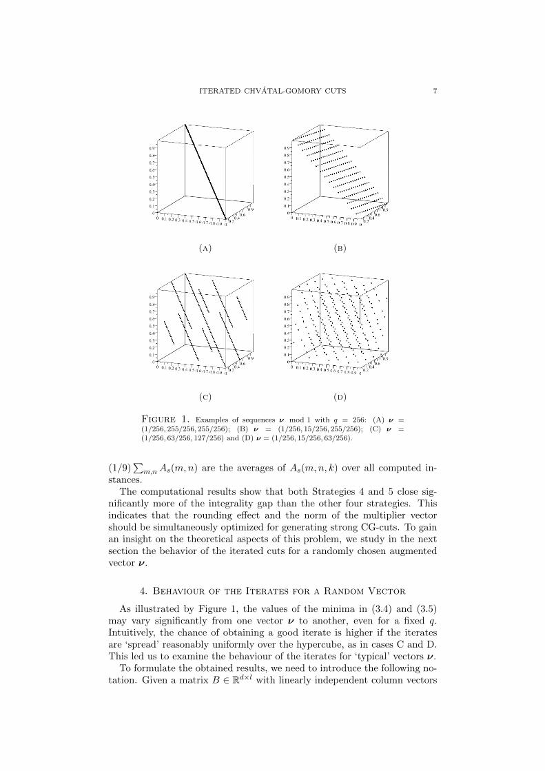
Figure 1. Examples of sequences ν mod 1 with q = 256: (A) ν =

(1/256, 255/256, 255/256); (B) ν = (1/256, 15/256, 255/256); (C) ν =(1/256, 63/256, 127/256) and (D) ν = (1/256, 15/256, 63/256).

(1/9)∑

m,nAs(m,n) are the averages of As(m,n, k) over all computed in-stances.

The computational results show that both Strategies 4 and 5 close sig-nificantly more of the integrality gap than the other four strategies. Thisindicates that the rounding effect and the norm of the multiplier vectorshould be simultaneously optimized for generating strong CG-cuts. To gainan insight on the theoretical aspects of this problem, we study in the nextsection the behavior of the iterated cuts for a randomly chosen augmentedvector ν.

4. Behaviour of the Iterates for a Random Vector

As illustrated by Figure 1, the values of the minima in (3.4) and (3.5)may vary significantly from one vector ν to another, even for a fixed q.Intuitively, the chance of obtaining a good iterate is higher if the iteratesare ‘spread’ reasonably uniformly over the hypercube, as in cases C and D.This led us to examine the behaviour of the iterates for ‘typical’ vectors ν.

To formulate the obtained results, we need to introduce the following no-tation. Given a matrix B ∈ Rd×l with linearly independent column vectors


b1, . . . , bl ∈ Rd, the set

L(b1, . . . , bl) = u1b1 + · · ·+ ulbl : u1, . . . , ul ∈ Z

is called a lattice of rank (or dimension) l with basis b1, . . . , bl and determi-nant

det(L(b1, . . . , bl)) =√

det(BTB) .

For a comprehensive and extensive survey on lattices and Minkowski’s geom-etry of numbers we refer the reader to the book of Gruber and Lekkerkerker[24].

Given lattice L, we will denote by L∗ its dual lattice, that is

L∗ = y ∈ spanR(L) : yTx ∈ Z for all x ∈ L .

Let Bd(x, r) denote a d-dimensional ball of radius r centered at x. Givenany l-dimensional lattice Λ ⊂ Rd we also denote by λi = λi(Λ) its ithsuccessive minimum

λi = minr > 0 : dim spanR(Bd(0, r) ∩ Λ) ≥ i , 1 ≤ i ≤ l .

Recall that the inhomogeneous minimum of a set S ⊂ spanR(L) withrespect to a lattice L is defined as

µ(S,L) = infσ > 0 : L+ σS = spanR(L) .

The covering radius τ(L) of a lattice L is the inhomogeneous minimum ofthe unit ball B in spanR(L) with respect to L,

τ(L) = µ(B,L) .

Let also d (resp. d) denote the Vinogradov symbol with the constantdepending on d only. The notationd is interpreted as bothd andd

hold.We will first study the ‘typical’ behaviour of the iterates, for a random

vector ν sampled from a certain natural distribution. In particular, we showthat the covering radius of a lattice associated with ν is relatively small onaverage. This is important because the quality of the approximation algo-rithm presented in Section 5 will be defined in terms of the covering radius.(Of course, a multiplier vector obtained in a real cutting-plane algorithmwill not be truly random. Nevertheless, the insights gained in this sectionwill be useful for what follows.)

In more detail, we study in this section the behavior of the points tνmod 1 for a random vector ν uniformly chosen from the set of rationalvectors of the form

ν =

(p1

q,p2

q, . . . ,

pdq

)T, p1, p2, . . . , pd, q ∈ Z>0 ,

max1≤i≤d

pi < q , gcd(p1, p2, . . . , pd, q) = 1(4.1)

that have denominator q ≤ T , for some T ≥ 1. Our aim is to understandhow well the points tν mod 1 are distributed ‘on average’.

The iterates tν mod 1 can be naturally embedded in the lattice

Lν = z + (tν mod 1) : z ∈ Zd , t = 1, . . . , q − 1 .(4.2)


Equivalently, Lν = Zd + Zν. This observation allows us to use results fromMinkowski’s geometry of numbers and, via the transference principle (see,e.g., [7]), Schmidt’s theorems [40] on the distribution of integer sublattices.

The first result of this paper aims to understand the ‘typical’ behavior ofthe covering radius τ(Lν) for ν of the form (4.1) with common denominatorq ≤ T . Note that for any dimension d and any common denominator q > 1there exist vectors ν such that the covering radius τ(Lν) is relatively large.For instance, it is easy to see that τ(L(1/q,...,1/q)) > 1/4 for any integer q > 1.In what follows, we will show that for a ‘typical’ vector ν the covering radiusτ(Lν) has the order q−1/d.

For technical reasons it is convenient to replace the rationals with boundeddenominators by the primitive integer vectors in a bounded domain. Let

Nd+1 be the set of integer vectors in Rd+1 with positive co-prime coefficients,and let

Dd+1 =

(x1, . . . , xd, xd+1) ∈ Rd+1

≥0 : maxj=1,...,d

xj < xd+1 ≤ 1

.

Then for T ≥ 1, the elements a = (p1, . . . , pd, q) of the set Nd+1 ∩ TDd+1

will correspond to the rational vectors ν of the form (4.1) and the commondenominator q ≤ T . Since Lν is uniquely defined by the integer vectora = (p1, . . . , pd, q), we will also denote the lattice Lν by La.

For any T ∈ R≥1 and R ∈ R>0, we define the quantity

Pd(T,R) =1

#(Nd+1 ∩ TDd+1)#a ∈ Nd+1 ∩ TDd+1 : τ(La)a

1/dd+1 > R

.

Roughly speaking, Pd(T,R) is the probability of uniformly picking up arational vector ν of the form (4.1) with denominator q ≤ T , such thatthe iterations tν mod 1 are relatively badly distributed in [0, 1)d or, moreprecisely, such that the covering radius of the lattice Lν is bigger thanRq−1/d.

Theorem 4.1. Let d ≥ 2. Then

Pd(T,R)d R−d ,(4.3)

uniformly over all T ≥ 1 and all R > 0. Furthermore,

Pd(T,R) = 0 whenever R >

√d

2T 1/d .(4.4)

A celebrated result of Kannan [29] implies that the Frobenius number

associated with an integer vector a ∈ Nd+1 can be estimated in terms of thecovering radius of the dual lattice L∗a. (For more details we refer the readerto the book of Ramirez Alfonsin [39].) The following proof of Theorem4.1 is based on a recent far-reaching refinement due to Strombergsson [45]of the approach used in [2] and [3] for estimating the expected value ofFrobenius numbers, combined with the Banaszczyk transference theorem[7]. The approach is built on results from the Minkowski’s geometry ofnumbers (see e. g. [23], [24]) and results on the distribution of integerlattices obtained by Schmidt in [40].


Proof of Theorem 4.1. Observe that Zd is a sublattice of La and hence

τ(La) ≤ τ(Zd) =

√d

2.(4.5)

Note also that for all a ∈ Nd+1 ∩ TDd+1 we have ad+1 ≤ T . Hence theinequality (4.5) implies (4.4).

Let us now prove that the inequality (4.3) holds. For a subset Y ⊂ Rd+1

we denote by πd+1(Y ) the orthogonal projection of Y onto the coordinate

hyperplane xd+1 = 0; we view πd+1(Y ) as a subset of Rd. Given a ∈ Nd+1,we define the lattice

Λa = x ∈ Zd+1 : xTa = 0

and set Ma = πd+1(Λa). Then Ma is a sublattice of Zd of determinantdet(Ma) = ad+1 (see e. g. [1], Section 2) It is well-known that Ma = L∗a(see e.g. [1]).

By Banaszczyk transference theorem [7], we have

λ1(Ma) ≤ d

2τ(La).

Since Ma embedded in Rd+1 is the orthogonal projection of Λa on thecoordinate hyperplane xd+1 = 0 and ad+1 = maxi ai, we have λ1(Λa) ≤√d+ 1λ1(Ma) and, consequently,

λ1(Λa) ≤ d√d+ 1

2τ(La).(4.6)

In the rest of this subsection we modify the proof of Theorem 3 in [45]for our case. Roughly speaking, the main difference is that, due to thetransference principle reflected in the inequality (4.6), we need to work withthe first successive minimum λ1(Λa), whilst in the case of the Frobeniusnumber the last successive minimum λd(Λa) plays the major role.

Note first that #(Nd+1 ∩ TDd+1) d Td+1 uniformly over all T ≥ 1

and that det(Λa) = ||a|| ≥ ad+1. Therefore

Pd(T,R)d T−(d+1)×

×#

Λ ∈ Ld : det(Λ) ≤

√d+ 1T, λ1(Λ) <

d√d+ 1 det(Λ)1/d

2R

,

(4.7)

where Ld is the set of all d-dimensional sublattices of Zd+1.Let

ρj(Λ) = λj+1(Λ)/λj(Λ) , j = 1, . . . , d− 1 .

For any r = (r1, . . . , rd−1) ∈ Rd−1≥1 we set

Ld(r) = Λ ∈ Ld : ρj(Λ) ≥ rj , 1 ≤ j ≤ d− 1 .

Let also Xd be the set of all lattices L ⊂ Rd of determinant one and µd beSiegel’s measure (see [43]) on Xd, normalized to be a probability measure.The main ingredient of the proof is the following result.


Theorem 4.2 (Schmidt [40]). For any r ∈ Rd−1≥1 and T > 0 we have

#Λ ∈ Ld(r) : det(Λ) ≤ T =π

d+12

2Γ(1 + d+1

2

) d∏j=2

ζ(j)

××µd (L ∈ Xd : ρj(L) ≥ rj , 1 ≤ j ≤ d− 1)T d+1

+Od

d−1∏j=1

r−(j− 1

d)(d−j)

j

T d+1− 1d

.

(4.8)

Furthermore,

µd(L ∈ Xd : ρj(L) ≥ rj , 1 ≤ j ≤ d− 1)d

d−1∏j=1

r−j(d−j)j .(4.9)

From the above theorem we get the upper bound

# Λ ∈ Ld(r) : det(Λ) ≤ T d Td+1×

×d−1∏j=1

r−j(d−j)j

1 + T−1d

d−1∏j=1

r1d

(d−j)j

.(4.10)

By Minkowski’s Second theorem, for any d-dimensional lattice Λ we have

λ1(Λ)d =

∏dj=1 λj(Λ)∏d−1

j=1 ρj(Λ)d−jd

det(Λ)∏d−1j=1 ρj(Λ)d−j

.(4.11)

Thus there exists a constant c1 = c1(d) > 0 such that for any d-dimensionallattice Λ and any R > 0, we have

λ1(Λ) <d√d+ 1 det(Λ)1/d

2R⇒

d−1∏j=1

ρj(Λ)d−j > c1Rd .(4.12)

Assume without loss of generality R > ec− 1

d1 (the inequality (4.3) is trivial

when R 1 as Pd(T,R) ≤ 1), put

B = blog(c1Rd)− dc ∈ Z≥0 ,(4.13)

and denote

R(d,R) = (eb1/(d−1), eb2/(d−2), . . . , ebd−2/2, ebd−1) :

b ∈ Zd−1≥0 ,

d−1∑j=1

bj = B .(4.14)

If Λ is an d-dimensional lattice with∏d−1j=1 ρj(Λ)d−j > c1R

d, then for bj =

b(d− j) log ρj(Λ)c we have

d−1∑j=1

bj >

d−1∑j=1

((d− j) log ρj(Λ)− 1) > log(c1Rd)− (d− 1)

> log(c1Rd)− d ≥ B .

(4.15)


Thus we can decrease some of the numbers bj ’s so as to make∑d−1

j=1 bj = B,

while keeping b = (b1, . . . , bd−1) ∈ Zd−1≥0 . The new vector b still satisfies

bj ≤ (d − j) log ρj(Λ) for each j, that is ρj(Λ) ≥ ebj/(d−j). Therefore, for

any d-dimensional lattice Λ with∏d−1j=1 ρj(Λ)d−j > c1R

d, there exists some

r ∈ R(d,R) such that rj ≤ ρj(Λ) for all j.By (4.12), the set in the right hand side of (4.7) is contained in the union

of Ld(r) over all r ∈ R(d,R). Hence we have for all T ≥ 1 and all R ≥ ec1d1 ,

Pd(T,R)d T−(d+1)×

×∑

r∈R(d,R)

#

Λ ∈ Ld(r) : det(Λ) ≤√d+ 1T

.(4.16)

By (4.10),

Pd(T,R)d

∑b ∈ Zd−1

≥0

b1 + . . .+ bd−1 = B

exp

−d−1∑j=1

jbj

+T−

1d

∑b ∈ Zd−1

≥0

b1 + . . .+ bd−1 = B

exp

−d−1∑j=1

(j − 1

d

)bj

.

(4.17)

If d = 2 we get

P2(T,R) R−2 + T−12R−1.

If R ≤√

22 T

1/2 then this implies P2(T,R) R−2. On the other hand, if

R >√

22 T

1/2 then P2(T,R) = 0 by (4.4).

Let us now assume d ≥ 3. Observe that for any b ∈ Zd−1≥0 with b1 + . . .+

bd−1 = B and b2 + . . .+ bd−1 = s, we have

d−1∑j=1

jbj ≥ B + s

and

d−1∑j=1

(j − 1

d

)bj ≥

(1− 1

d

)B + s .

Next, for s ∈ 0, 1, . . . , B there are exactly(s+d−3d−3

)vectors b ∈ Zd−1

≥0 withb1 + . . .+ bd−1 = B and b2 + . . .+ bd−1 = s. Therefore

Pd(T,R)d

B∑s=0

(s+ d− 3

d− 3

)e−B−s

+T−1d

B∑s=0

(s+ d− 3

d− 3

)e−(1− 1

d)B−s d e−B + T−

1d e−(1− 1

d)B

d R−d(1 + T−

1dR) .


If R ≤√d

2 T1/d then this implies Pd(T,R) R−d. On the other hand, if

R >√d

2 T1/d then Pd(T,R) = 0 by (4.4). The proof is complete.

5. The Approximation Algorithm

We will assume for this section that d ≥ 2. Theorem 4.1 shows that thequantity 1/q1/d is a good predictor for the covering radius of the lattice Lν .Let S = [0,+∞)d−1 × (−∞, 1). The following result states the existence ofa polynomial-time algorithm which computes a point of the set Lν ∩ S in acertain ball of radius bounded in terms of τ(Lν). The obtained bound willbe used to estimate the quality of polynomial-time approximations for themultiplicative and additive strategies (i.e., Strategies 4 and 5) introduced inSection 3.

For r ∈ R set

c(r) = (r, . . . , r, 1− r) ∈ Rd .

Theorem 5.1. There is a polynomial time algorithm which, given a rationalvector ν of the form (4.1) and any rational ε ∈ (0, 1), finds a point ξ ∈Lν ∩ S, such that

ξ ∈ B(c(r), 2d/2τ(Lν)) with 0 < r ≤ 2d/2τ(Lν) + ε .(5.1)

The proof is constructive. We present the polynomial time algorithm inSection 5.1.

5.1. Proof of Theorem 5.1. .We need to find in polynomial time a point of the set Lν ∩ S in a ball

Bd(c(r), r). The main challenge of the proof is to choose the radius r d

τ(Lν) as small as possible. Note that computing the covering radius of alattice is conjectured in [35] to be NP-hard (see also [27], [25] and [15]). TheBanaszczyk transference theorem [7] gives the estimate

τ(Lν) ≤ d

2λ1(L∗ν),

which allows to approximate τ(Lν) in polynomial time within the factor

d2d/2−1 using the celebrated LLL algorithm [31]. The approximation can bethen used for computing a relatively small radius r.

In this paper we use a slightly different approach. We will choose a suit-able radius r by combining binary search in a certain interval with Babai’snearest plane algorithm. The nearest plane algorithm finds in polynomialtime an approximation to a solution of the closest vector problem. Thequality of the approximation is given by the following result.

Theorem 5.2 (Babai [5]). Let L be a lattice of rank d in Qd. Given anybasis of L and any c ∈ Qd as input, the nearest plane algorithm computes avector x ∈ L such that

||x− c|| ≤ 2d/2 miny∈L||y − c|| .(5.2)


Babai’s nearest plane algorithm is based on using the LLL algorithmand, in fact, makes use also of the transference principle, via Gram-Schmidtorthogonalization. Note also that the approximation factor 2d/2 in (5.2) can

be replaced by 2O(d(log log d)2/ log d) by applying the algorithm of Schnorr [41].We shall now give a high level description of a polynomial-time algorithm

that satisfies conditions stated in Theorem 5.1. Given rational ν of the form(4.1), we first compute a basis u1,u2, . . . ,ud of the Lν . To perform this step,we use a link between iterations of ν modulo one and the computationalDiophantine approximations. Next we use a version of binary search to findin the interval [0, 1] two rationals r− and r+ with r− < r+, satisfying thefollowing properties. First, the numbers r−, r+ are relatively close to eachother, so that r+− r− < ε. Second, Babai’s nearest plane algorithm appliedto u1,u2, . . . ,ud and c = c(r+) finds a lattice point ξ ∈ Lν such that ξ ∈ Sand the same algorithm applied to u1,u2, . . . ,ud and c = c(r−) fails to finda lattice point in S. This will imply that ξ satisfies conditions of Theorem5.1.

The algorithm is given below.

Algorithm

Input : ν of the form (4.1) and rational ε ∈ (0, 1).Output : ξ ∈ Lν satisfying conditions of Theorem 5.1.Step 0 : Set r− := 0, r+ := 1 and ξ := c(1).Step 1 : Compute a basis u1,u2, . . . ,ud of the lattice Lν .Step 2 : While r+ − r− > ε do

2.1 Set m := (r− + r+)/2 and c := c(m).2.2 Apply the Babai’s algorithm for finding a nearby lattice point

to the basis u1, . . . ,ud and the point c. The algorithm returnsa lattice point χ ∈ Lν .

2.3 If χ ∈ S then set r+ := m else set r− := m end if.end while.

Step 3 : Output vector ξ.

Let us now analyze the algorithm. Clearly, Step 0 can be done in poly-nomial time. In Step 1 we can compute a basis of Lν as follows. Considerthe matrix G(ν) ∈ Qd×(d+1) defined as

G(ν) =

1 0 . . . 0 p1/q0 1 . . . 0 p2/q...

.... . .

......

0 0 . . . 1 pd/q

and denote by gi its ith column vector. Observe that Lν = y1g1 + . . . +yd+1gd+1 : y1, . . . , yd+1 ∈ Z. Thus we can find a basis of Lν in polynomialtime by Corollary 5.4.8 of [22] (see also [8]).

The while loop at Step 2 is performing a binary search in the interval [0, 1]with approximation error bounded by ε and thus will be executed O(l(ε))times, where l(ε) is the length of the binary expansion of the rational numberε. The algorithm of Babai (see [5]), applied at Step 2.2, runs in polynomialtime. Step 2.3 can be done in polynomial time as well.


Thus it is now enough to show that the vector ξ output at Step 3 sat-isfies conditions of Theorem 5.1. By Theorem 5.2, we clearly have ξ ∈B(c(r+), 2d/2τ(Lν)). Next, since Babai’s algorithm applied to u1, . . . ,udand the point c(r−) returns a lattice point outside of S, we also conclude

by Theorem 5.2 that r− ≤ 2d/2τ(L). The latter inequality together withr+ − r− ≤ ε implies then

r+ ≤ 2d/2τ(L) + ε .

Therefore the point ξ satisfies conditions of Theorem 5.1.Remark. It is easy to see that, in fact, we are solving in the above

proof a problem of simultaneous Diophantine approximation of rationalsp1/q, . . . , pd/q. Indeed, all points of the lattice Lν have the form (y1 −yd+1p1/q, . . . , yd−yd+1pd/q) with integer numbers yi. It may also be worth-while using another standard approach to computing Diophantine approx-imations with bounded denominators for a given rational vector. In thiscase, we construct a basis of a special lattice Ω ∈ Qd+1 with πd+1(Ω) = Lν .For details, see the proof of Theorem 5.3.19 in [22] or, for a more recentapproach, Chapter 6 in [31].

5.2. Approximation for the multiplicative strategy. For the rest ofthe paper we set d = m+ 1. Given the multiplier vector λ of the form (3.1),we construct the augmented vector

ν = (λ1, . . . , λm, ν)T ∈ (0, 1)d,

and attempt to find a vector ξ = tν mod 1, ξd > 0, with minimum ratio

r(ξ) = ||πd(ξ)||/ξd .Recall that for Y ⊂ Rd by πd(Y ) we understand the orthogonal projectionof Y onto the coordinate hyperplane xd = 0; we view πd(Y ) as a subset ofRd−1.

As it was remarked in Section 4, for any given common denominatorq > 1 there exist rational vectors ν of the form (4.1) with τ(Lν) 1.However, due to Theorem 4.1, for a typical ν the covering radius of thelattice Lν is of order q−1/d. In the following we show the existence of avector ξ = tν mod 1, with ratio r(ξ) bounded in terms of the coveringradius. We also show the existence of a polynomial-time algorithm whichcomputes an approximation of that vector ξ.

For 0 < R < 1/2 set

a(d,R) =(1−R)((d− 1)R2 − 2R+ 1)1/2 − (d− 1)1/2R2

dR2 − 2R+ 1

and

r(d,R) =

(a(d,R)−2 − 1)1/2 for 0 < R < 1/2 ,+∞ otherwise .

We will first prove a simple geometric lemma.

Lemma 5.1. Let 0 < R < 1/2. Then

maxr(x) : x ∈ Bd(c(R), R) = r(d,R) .(5.3)


Proof. For any fixed 1−R ≤ y ≤ 1 , the maximum

maxr(x) : x = (x1, . . . , xd−1, y) ∈ Bd(c(R), R)

is attained at a point of the form (x, . . . , x, y). Thus we can consider only twovariables, x and y, and (5.3) reduces to solving a 2-dimensional trigonometricproblem. Straightforward computation gives

max

√d− 1 x

y: (x, . . . , x, y) ∈ Bd(c(R), R)

= r(d,R) .(5.4)

By (5.4), we also have r(d,R)d R when 0 < R < 1/2.

Proposition 5.1. There exists a point ξ = tν mod 1, 1 ≤ t ≤ q − 1, with

r(ξ) ≤ minr(d, τ(Lν)), 2√d− 1 .(5.5)

Proof. Observe first that there is a positive integer t0 such that 1/2 ≤t0ν < 1. Thus for ξ = t0ν mod 1, we have

r(ξ) < 2√d− 1 .

This justifies the second bound in (5.5).Recall that the iterations tν mod 1 can be naturally embedded in the

lattice Lν . Thus, it is enough to show that there exists a nonzero pointξ ∈ Lν ∩ [0, 1)d that satisfies the first inequality in (5.5). If τ(Lν) ≥ 1/2, thelatter inequality holds by the definition of r(d,R). Suppose that τ(Lν) <1/2. By the definition of the covering radius there exists a point ξ ∈ Lν ∩Bd(c(τ(Lν)), τ(Lν)). Since τ(Lν) < 1/2, the point ξ is in [0, 1)d. The firstinequality in (5.5) now holds by Lemma 5.1.

On the algorithmic side, Theorem 5.1 implies the following result.

Corollary 5.1. There is a polynomial-time algorithm which, given an aug-mented vector ν = (λ1, . . . , λm, ν) of the form (4.1) and any rational ε ∈(0, 1), finds a point ξ = tν mod 1, 1 ≤ t ≤ q − 1, with

r(ξ) < minr(d, 2d/2τ(Lν) + ε), 2√d− 1 .(5.6)

Proof. The first bound in (5.6) immediately follows from Theorem 5.1 and

Lemma 5.1, where we take R = 2d/2τ(Lν) + ε.Next, if ν ≥ 1/2, we have r(ν) < 2

√d− 1, so the second bound in (5.6)

holds for ξ = ν. If 0 < ν < 1/2, then we can take ξ = t0ν mod 1 witht0 = b1/νc when b1/νcν 6= 1 and t0 = b1/νc − 1 otherwise.

5.3. Approximation for the additive strategy. Now we move on tothe additive strategy. As in the previous section, for a non-trivial CG-cut(1.1) with λ of the form (3.1) we construct the augmented vector ν =(λ1, . . . , λm, ν)T . One can easily obtain the following bound for Problem3.5.


Proposition 5.2. There exists a point ξ = tν mod 1, 1 ≤ t ≤ q − 1, with

N(ξ) ≤ (1 +√d)τ(Lν) .(5.7)

Furthermore,

tν > 0 whenever τ(Lν) < 1/2 .(5.8)

Proof. Observe that the set Bd(c(0), (1 +√d)τ(Lν)) ∩ S contains the ball

Bd(c(τ(Lν)), τ(Lν)). By the definition of the covering radius there exists

a point χ ∈ Lν ∩ Bd(c(τ(Lν)), τ(Lν)), so that N(χ) ≤ (1 +√d)τ(Lν).

If χ ∈ Zd then we may assume without loss of generality that χ = c(1).Thus in this case we can take ξ = ν. Otherwise, since χ ∈ S \ Zd, wehave 0 < N(χ mod 1) ≤ N(χ). Thus, the point ξ = χ mod 1 satisfiescondition (5.7).

Suppose now that τ(Lν) < 1/2. Then for all sufficiently small ε > 0the ball Bd(c((τ(Lν) + ε)), τ(Lν)) contains a point of the set Lν ∩ (0, 1)d.Since Lν is a discrete set, we conclude that there exists a point ξ ∈ Lν ∩Bd(c(τ(Lν)), τ(Lν)) ∩ (0, 1)d. This point clearly satisfies (5.8).

On the other hand, Theorem 5.1 implies the following

Corollary 5.2. There is a polynomial-time algorithm which, given an aug-mented vector ν = (λ1, . . . , λm, ν) of the form (4.1) and any rational δ ∈(0, 1), finds a point ξ = tν mod 1, 1 ≤ t ≤ q − 1, with

N(ξ) < (1 +√d)2d/2τ(Lν) + δ .(5.9)

Furthermore,

tν > 0 whenever τ(Lν) < 2−d/2−1(1− δ/d√de) .(5.10)

Proof. By Theorem 5.1, given ν = (λ1, . . . , λm, ν) and ε = δ/d√de ∈ (0, 1)

we can compute in polynomial time a point ξ ∈ Lν ∩ S such that ξ ∈B(c(r), 2d/2τ(Lν)) with 0 < r ≤ 2d/2τ(Lν) + ε. Thus N(ξ) ≤ N(c(r)) +

2d/2τ(L) and, consequently,

N(ξ) ≤ (2d/2τ(L) + ε)√d+ 2d/2τ(L) ≤ (1 +

√d)2d/2τ(L) + δ.

Therefore the point ξ satisfies the inequality (5.9).

Suppose now that τ(Lν) < 2−d/2−1(1− δ/d√de). Clearly, tν = ξd, so

it is enough to show that ξd ∈ (0, 1). Since ξ ∈ S, the number ξd is positive.On the other hand, we have

ξd ≤ r + 2d/2τ(L) ≤ 2d/2+1τ(L) + δ/d√de < 1 .

5.4. Approximation error. As it is shown in Sections 5.2 and 5.3, thecomputed approximations of the optimal values of r(ξ) andN(ξ) are boundedin terms of the covering radius and thus are small for a typical augmentedvector. We conjecture that the iterated CG-cuts found by the algorithmsobtained in Corollaries 5.1 and 5.2 solve problems (3.4) and (3.5), respec-

tively, with the multiplicative approximation error 2O(d). In this section we


prove the second conjecture for the special case τ(Lν) q−1/d, where isthe Vinogradov symbol.

Let ν = (λ1, . . . , λm, ν) be a vector of the form (4.1) and let δ ∈ (0, 1)∩Q.We will denote by madd = madd(ν) the value of the minimum in (3.5), thatis

madd(ν) = min N(tν mod 1) : t = 1, . . . , q − 1, tν > 0 .We will also denote by ξadd = ξadd(ν, δ) the output vector of the algorithmobtained in Corollary 5.2.

Proposition 5.3. Let ν be a vector of the form (4.1) with common denom-inator q. Then

N(ξadd(ν, 1/q))

madd(ν)< 23d/2−1(1 +

√d)τ(Lν)dq + 1 .(5.11)

Proof. Recall that Lν = Zd+Zν. Therefore for the first successive minimumλ1 = λ1(Lν) we obtain the inequalities 1/q ≤ λ1 ≤ madd(ν). Together with(5.9) this observation implies the inequality

N(ξadd(ν, 1/q))

madd(ν)<

(1 +√d)2d/2τ(Lν)

λ1+ 1 .(5.12)

By Minkowski’s Second theorem for spheres, 1/q = det(Lν) ≤ λ1λ2 · · ·λdand hence

λ1 ≥1

qλd−1d

.(5.13)

Next, by Jarnik’s inequalities (cf. [24, p. 99, p. 106])) we have λd ≤ 2τ(Lν).Consequently, by (5.13)

λ1 ≥1

2d−1qτ(Lν)d−1.(5.14)

Combining (5.12) and (5.14), we obtain the inequality (5.11).

Proposition 5.3 immediately implies the inequality N(ξadd(ν, 1/q)) <

2O(d)madd(ν), provided τ(Lν) q−1/d.A natural step towards establishing both conjectures would be to show

that the approximation error is independent of the common denominatorq. In this light, Proposition 5.3, together with Theorem 4.3 imply that fora typical input vector ν the problem (3.5) can be approximated with themultiplicative approximation error that only depends on d.

6. Concluding Remarks

Although Chvatal-Gomory cuts have been around for over 50 years andhave been studied in depth, many important questions about them remainunanswered. We have studied the behavior of the iterated CG-cuts fora randomly chosen augmented vector and have shown the existence of apolynomial-time algorithm that computes approximations for the problems3.4 and 3.5. For computed approximations the values of r(ξ) and N(ξ)


are bounded in terms of the covering radius and thus are small for a typ-ical augmented vector. On the other hand, we do not know the preciseapproximation ratio that this algorithm yields. Nor do we know the pre-cise approximability (or inapproximability) status of the problems 3.4 and3.5. Moreover, our algorithm seems at present of mainly theoretical interest,though this may change in the near future, given the intensive recent workon algorithms for integer lattices (see the survey [26]).

We also remark that the strategy presented in this paper is designed tooptimize individual CG-cuts only. On the other hand, since the work ofBalas et al. [6], most integer programmers prefer to work with collections ofcutting planes rather than individual ones. (Specifically, given a fractionalsimplex tableau, one can generate one GF-cut for each fractional variable,and add all such GF-cuts to the LP relaxation.) It is not clear that optimis-ing each CG-cut in a collection will improve the effectiveness of the entirecollection. Indeed, in our computational experiments, we often observedthat different CG-cuts led to the same strengthened iterated CG-cut, sothat a large collection of weak CG-cuts was converted into a small collectionof strong ones. This suggests that a suitable topic for future research mightbe the simultaneous optimization of a collection of CG-cuts. A methodfor strengthening a collection of Gomory mixed-integer cuts, rather thanGF-cuts, was presented in [4].

References

[1] I. Aliev, P.M. Gruber, Best simultaneous Diophantine approximations under a con-straint on the denominator. Contrib. Discr. Math. 1 (2006) 29–46.

[2] I. Aliev, M. Henk, Integer knapsacks: average behavior of the Frobenius numbers.Math. Oper. Res. 34 (2009) 698–705.

[3] I. Aliev, M. Henk, A. Hinrichs, Expected Frobenius numbers. J. Comb. Th. A 118(2011) 525–531.

[4] K. Andersen, G. Cornuejols, Y. Li, Reduce-and-split cuts: improving the performanceof mixed-integer Gomory cuts. Management Science, 51 (2005) 1720–1732.

[5] L. Babai, On Lovasz’ lattice reduction and the nearest lattice point problem. Combi-natorica 6 (1986) 1–13.

[6] E. Balas, S. Ceria, G. Cornuejols, N. Natraj, Gomory cuts revisited. Oper. Res. Lett.19 (1996) 1-9.

[7] W. Banaszczyk, New bounds in some transference theorems in the geometry of num-bers. Mathematische Annalen 296 (1993) 625-635.

[8] J. Buchmann, M. Pohst, Computing a lattice basis from a system of generating vectors,Proceedings of EUROCAL 1987, Lecture Notes in Computer Science 378 (1987) 54–63.

[9] A. Caprara, M. Fischetti, 0, 12-Chvatal-Gomory cuts. Math. Prog. 74 (1996) 221–

235.[10] A. Caprara, M. Fischetti, A.N. Letchford, On the separation of maximally violated

mod-k cuts. Math. Prog. 87 (2000) 37-56.[11] S. Ceria, G. Cornuejols, M. Dawande, Combining and strengthening Gomory cuts. In

E. Balas & J. Clausen (eds.), Proceedings of IPCO 1995, pp. 438–451.[12] W. Cook, R. Kannan, A.J. Schrijver, Chvatal closures for mixed integer programming

problems. Math. Program. 47 (1990) 155-174.[13] V. Chvatal, Edmonds polytopes and a hierarchy of combinatorial problems. Discr.

Math. 4 (1973) 305-337.[14] S. Dash, O. Gunluk, Valid inequalities based on simple mixed-integer sets. Math.

Program. 105 (2006) 29–53.


[15] M. Dutour Sikiric, A. Schurmann, F. Vallentin, Complexity and algorithms for com-puting Voronoi cells of lattices, Math. Comp. 78 (2009) 1713-1731.

[16] F. Eisenbrand, On the membership problem for the elementary closure of a polyhedron.Combinatorica 19 (1999) 297–300.

[17] F. Eisenbrand, Integer programming and algorithmic geometry of numbers, 50 Yearsof Integer Programming 1958-2008 (2010): 505–559.

[18] M. Fischetti, A. Lodi, Optimizing over the first Chvatal closure. Math. Prog. 110(2007), 3–20.

[19] R.E. Gomory, Outline of an algorithm for integer solutions to linear programs. Bull.Amer. Math. Soc. 64 (1958) 275-278.

[20] R.E. Gomory, An algorithm for integer solutions to linear programs. In: R.L. Graves& P. Wolfe (eds.), Recent Advances in Mathematical Programming. McGraw-Hill,New York, 1963.

[21] R.E. Gomory, An algorithm for the mixed-integer problem. Report RM-2597, RandCorporation (unpublished) (1963).

[22] M. Grotschel, L. Lovasz, A. Schrijver, Geometric Algorithms and Combinatorial Op-timization, Algorithms and Combinatorics vol. 2, Springer-Verlag, Berlin, 1988.

[23] P.M. Gruber, Convex and Discrete Geometry, Springer, Berlin, 2007.[24] P.M. Gruber, C.G. Lekkerkerker, Geometry of Numbers, North–Holland, Amsterdam

1987.[25] V. Guruswami, D. Micciancio, O. Regev, The complexity of the covering radius prob-

lem. Comput. Complexity 14 (2005) 90-121.[26] G. Hanrot, D. Stehle, X. Pujol, Algorithms for the Shortest and Closest Lattice Vector

Problems, IWCC 2011, to appear.[27] I. Haviv, O. Regev, Hardness of the covering radius problem on lattices. Chic. J.

Theor. Comput. Sci., 2012. Preliminary version in CCC 2006.[28] E. Hlawka, Zur angenaherten Berechnung mehrfacher Integrale. Monatshefte fur

Mathematik 66 (1962) 150–151.[29] R. Kannan, Lattice translates of a polytope and the Frobenius problem, Combinatorica,

12(2)(1992), 161–177.[30] N.M. Korobov, The approximate computation of multiple integrals. Doklady Akademii

Nauk SSSR 124 (1959) 1207–1210.[31] A.K. Lenstra, H.W. Lenstra Jr., L. Lovasz, Factoring polynomials with rational coef-

ficients. Math. Ann. 261 (1982) 515–534.[32] A.N. Letchford, Totally tight Chvatal-Gomory cuts. Oper. Res. Lett. 30 (2002) 71–73.[33] A.N. Letchford, A. Lodi, Strengthening Chvatal-Gomory cuts and Gomory fractional

cuts. Oper. Res. Lett. 30 (2002) 74-82.[34] H. Marchand, A. Martin, R. Weismantel, L. A. Wolsey, Cutting planes in integer and

mixed integer programming, Discrete Appl. Math., 123 (2002) 397–446.[35] D. Micciancio, Almost perfect lattices, the covering radius problem, and applications

to Ajtais connection factor, SIAM J. on Comp., 34 (2004) 118–169.[36] G.L. Nemhauser, L.A. Wolsey, Integer and Combinatorial Optimisation, Chichester:

Wiley, 1988.[37] G.L. Nemhauser, L.A. Wolsey, A recursive procedure to generate all cuts for 01 mixed

integer programs. Math. Program. 46 (1990) 379–390.[38] P. Nguyen, B. Vallee (eds.), The LLL Algorithm. Springer-Verlag; Berlin–Heidelberg.

2010.[39] J. L. Ramırez Alfonsın, The Diophantine Frobenius problem, Oxford Lecture Series

in Mathematics and its Applications 30 (2005), xvi+243.[40] W.M. Schmidt, The distribution of sublattices of Zm. Monatsh. Math. 125 (1998)

37–81.[41] C.-P. Schnorr, A hierarchy of polynomial time lattice basis reduction algorithms,

Theor. Comput. Sci. 53 (1987) 201-224.[42] A. Schrijver, On cutting planes. Ann. Discr. Math 9 (1980) 291–296.[43] C.L. Siegel, A mean value theorem in geometry of numbers. Ann. Math. 46 (1945)

340–347.


[44] I. Sloan, S. Joe, Lattice Methods for Multiple Integration, Oxford University Press,New York and Oxford, 1994.

[45] A. Strombergsson, On the limit distribution of Frobenius numbers. Acta Arith. 152(2012) 81–107.

[46] L.A. Wolsey, Integer Programming. New York: Wiley.

School of Mathematics, Cardiff University, Cardiff, Wales, UKE-mail address: [email protected]

Department of Management Science, Lancaster University, Lancaster, UKE-mail address: [email protected]

Documents

ITERATED CHVATAL-GOMORY CUTS AND THE GEOMETRY OF NUMBERS · ITERATED CHVATAL-GOMORY CUTS AND THE GEOMETRY OF NUMBERS ISKANDER ALIEV AND ADAM LETCHFORD Abstract. Chv atal-Gomory cutting