Embed Size (px)
DESCRIPTION
Iterative Deepening. CPSC 322 – Search 6 Textbook § 3.7.3 January 24, 2011. Lecture Overview. Recap from last week Iterative Deepening. Search with Costs. Sometimes there are costs associated with arcs. In this setting we often don't just want to find any solution - PowerPoint PPT Presentation
Citation preview
Iterative Deepening
CPSC 322 – Search 6
Textbook § 3.7.3
January 24, 2011
Lecture Overview
• Recap from last week
• Iterative Deepening
Slide 2
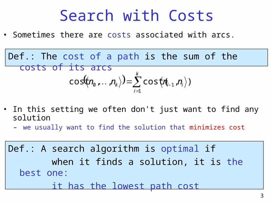
Search with Costs• Sometimes there are costs associated with arcs.
• In this setting we often don't just want to find any solution– we usually want to find the solution that minimizes cost
),cost(,,cost1
10
k
iiik nnnn
Def.: The cost of a path is the sum of the costs of its arcs
Def.: A search algorithm is optimal if when it finds a solution, it is the best one: it has the lowest path cost
3
• Expands the path with the lowest cost on the frontier.
• The frontier is implemented as a priority queue ordered by path cost.
• How does this differ from Dijkstra's algorithm?- The two algorithms are very similar- But Dijkstra’s algorithm
- works with nodes not with paths- stores one bit per node (infeasible for infinite/very large
graphs)- checks for cycles
Lowest-Cost-First Search (LCFS)
4
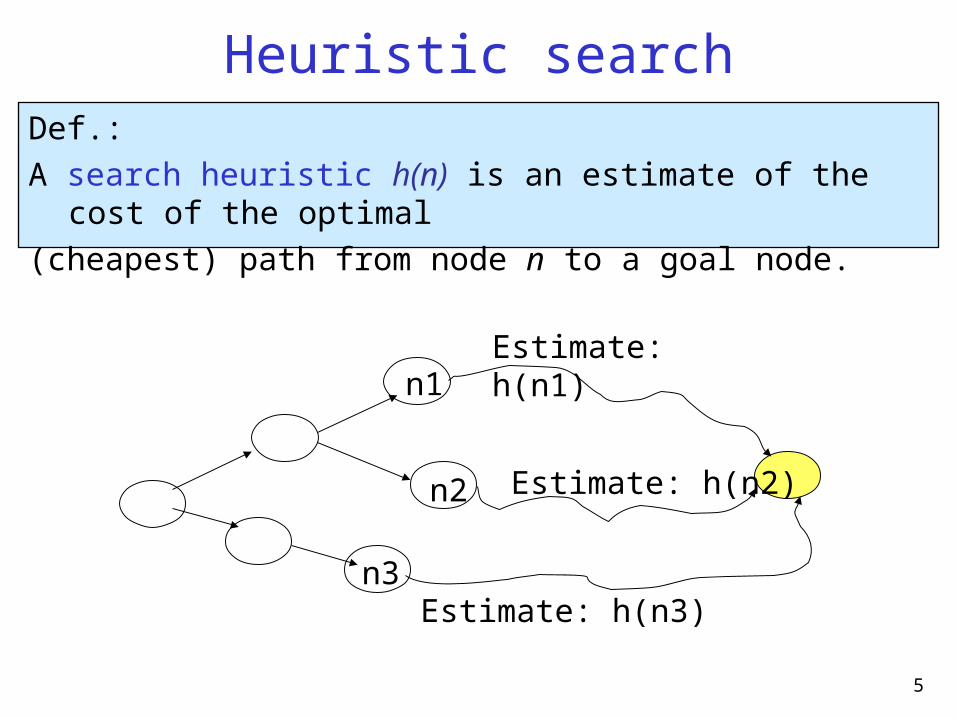
Heuristic searchDef.: A search heuristic h(n) is an estimate of the cost of the
optimal (cheapest) path from node n to a goal node.
Estimate: h(n1)
5
Estimate: h(n2)
Estimate: h(n3)n3
n2
n1
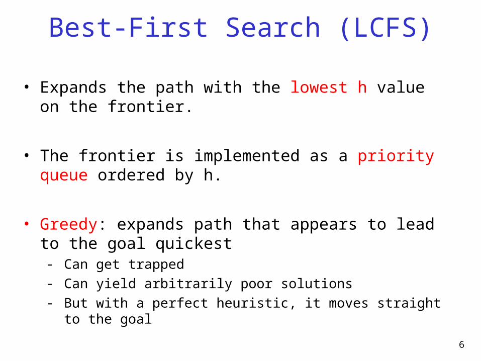
• Expands the path with the lowest h value on the frontier.
• The frontier is implemented as a priority queue ordered by h.
• Greedy: expands path that appears to lead to the goal quickest- Can get trapped- Can yield arbitrarily poor solutions- But with a perfect heuristic, it moves straight to the goal
Best-First Search (LCFS)
6
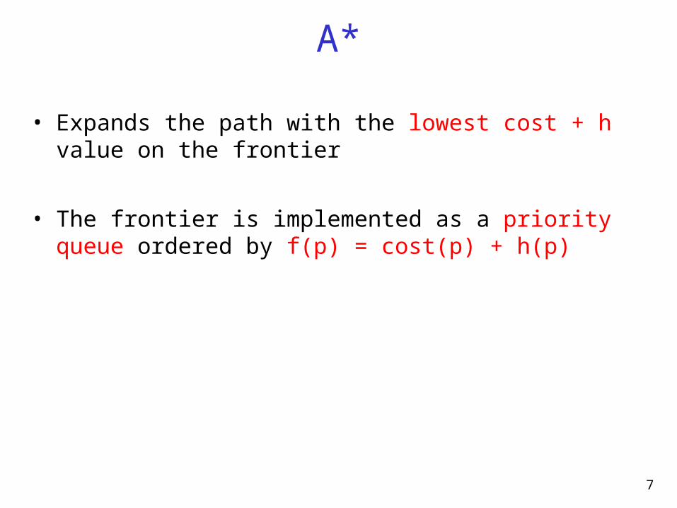
• Expands the path with the lowest cost + h value on the frontier
• The frontier is implemented as a priority queue ordered by f(p) = cost(p) + h(p)
A*
7
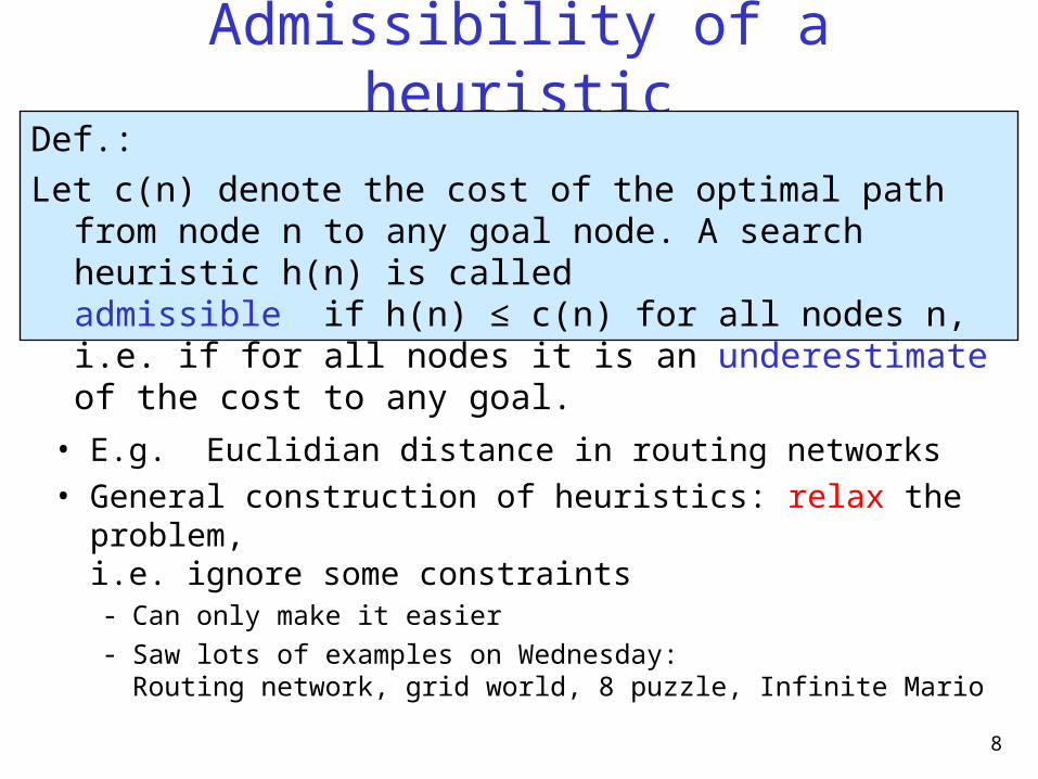
Admissibility of a heuristic
• E.g. Euclidian distance in routing networks• General construction of heuristics: relax the
problem, i.e. ignore some constraints- Can only make it easier- Saw lots of examples on Wednesday:
Routing network, grid world, 8 puzzle, Infinite Mario
8
Def.: Let c(n) denote the cost of the optimal path from node
n to any goal node. A search heuristic h(n) is called admissible if h(n) ≤ c(n) for all nodes n, i.e. if for all nodes it is an underestimate of the cost to any goal.
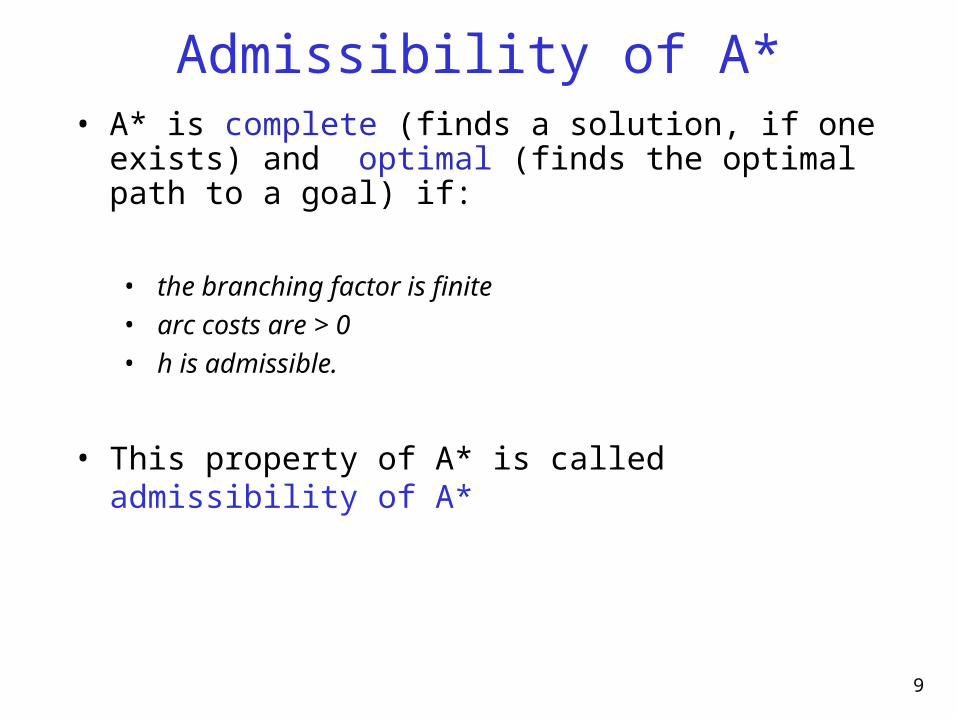
• A* is complete (finds a solution, if one exists) and optimal (finds the optimal path to a goal) if:
• the branching factor is finite• arc costs are > 0 • h is admissible.
• This property of A* is called admissibility of A*
Admissibility of A*
9
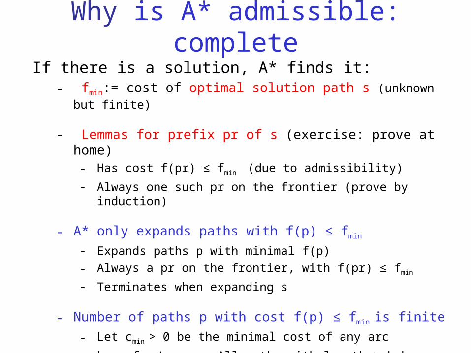
If there is a solution, A* finds it: - fmin:= cost of optimal solution path s (unknown but finite)
- Lemmas for prefix pr of s (exercise: prove at home)- Has cost f(pr) ≤ fmin (due to admissibility)
- Always one such pr on the frontier (prove by induction)
- A* only expands paths with f(p) ≤ fmin
- Expands paths p with minimal f(p)
- Always a pr on the frontier, with f(pr) ≤ fmin
- Terminates when expanding s
- Number of paths p with cost f(p) ≤ fmin is finite
- Let cmin > 0 be the minimal cost of any arc
- k := fmin / cmin. All paths with length > k have cost > fmin
- Only bk paths of length k. Finite b finite
Why is A* admissible: complete
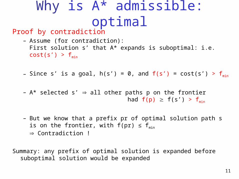
Why is A* admissible: optimalProof by contradiction
– Assume (for contradiction):First solution s’ that A* expands is suboptimal: i.e. cost(s’) > fmin
– Since s’ is a goal, h(s’) = 0, and f(s’) = cost(s’) > fmin
– A* selected s’ all other paths p on the frontier had f(p) f(s’) > fmin
– But we know that a prefix pr of optimal solution path s is on the frontier, with f(pr) ≤ fmin
Contradiction !
Summary: any prefix of optimal solution is expanded before suboptimal solution would be expanded
11
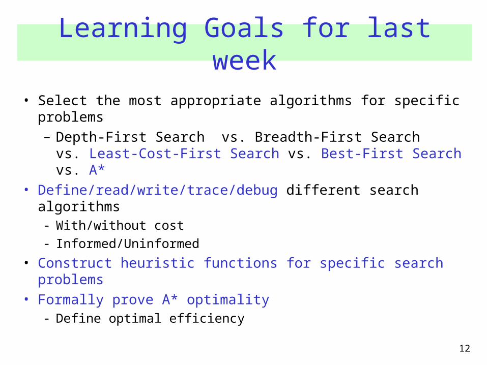
• Select the most appropriate algorithms for specific problems– Depth-First Search vs. Breadth-First Search
vs. Least-Cost-First Search vs. Best-First Search vs. A*• Define/read/write/trace/debug different search
algorithms- With/without cost- Informed/Uninformed
• Construct heuristic functions for specific search problems
• Formally prove A* optimality- Define optimal efficiency
12
Learning Goals for last week
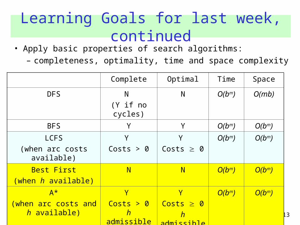
• Apply basic properties of search algorithms: – completeness, optimality, time and space complexity
13
Learning Goals for last week, continued
Complete Optimal Time Space
DFS N (Y if no cycles)
N O(bm) O(mb)
BFS Y Y O(bm) O(bm)
LCFS(when arc costs
available)
Y Costs > 0
Y Costs 0
O(bm) O(bm)
Best First(when h available)
N N O(bm) O(bm)
A*(when arc costs and h
available)
Y Costs > 0
h admissible
Y Costs 0
h admissible
O(bm) O(bm)
Lecture Overview
• Recap from last week
• Iterative Deepening
14
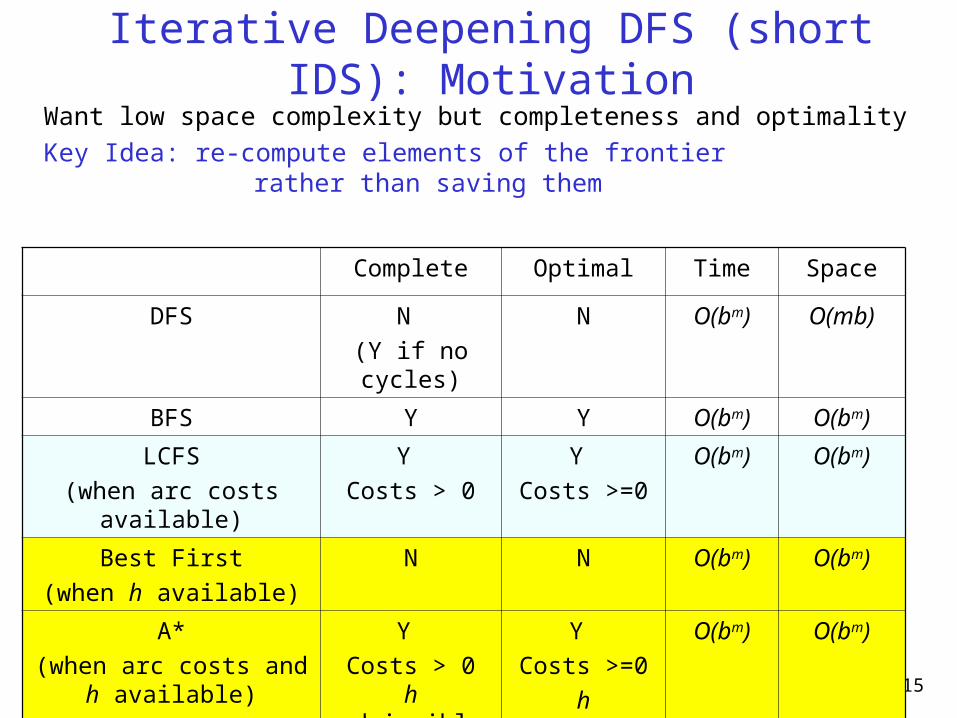
Want low space complexity but completeness and optimalityKey Idea: re-compute elements of the frontier
rather than saving them
15
Complete Optimal Time Space
DFS N (Y if no cycles)
N O(bm) O(mb)
BFS Y Y O(bm) O(bm)
LCFS(when arc costs
available)
Y Costs > 0
Y Costs >=0
O(bm) O(bm)
Best First(when h available)
N N O(bm) O(bm)
A*(when arc costs and h
available)
Y Costs > 0
h admissible
Y Costs >=0
h admissible
O(bm) O(bm)
Iterative Deepening DFS (short IDS): Motivation
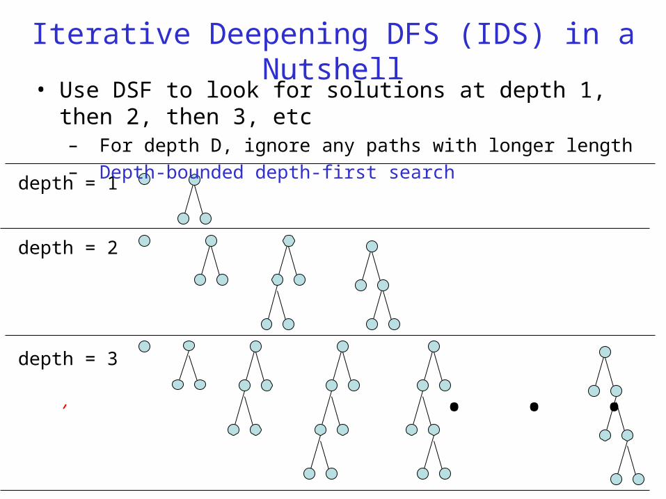
depth = 1
depth = 2
depth = 3
. . .
Iterative Deepening DFS (IDS) in a Nutshell
• Use DSF to look for solutions at depth 1, then 2, then 3, etc– For depth D, ignore any paths with longer length– Depth-bounded depth-first search
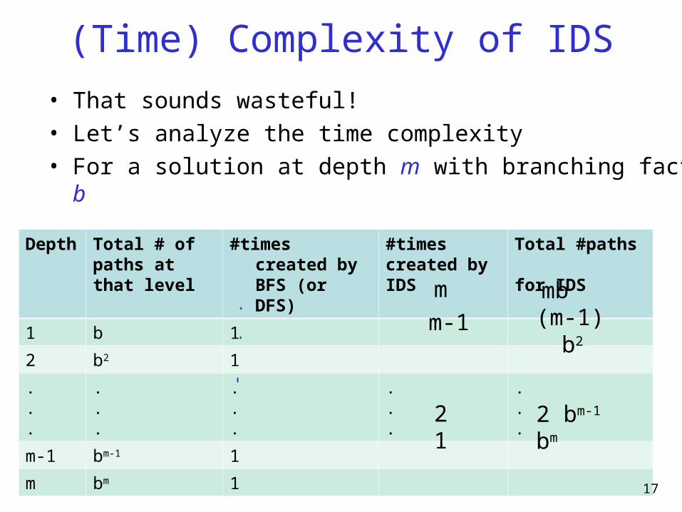
(Time) Complexity of IDS
Depth
Total # of paths at that level
#times created by BFS (or DFS)
#times created by IDS
Total #paths for IDS
1 b 1
2 b2 1
.
.
.
.
.
.
.
.
.
.
.
.
.
.
.
m-1 bm-1 1
m bm 1 17
mm-1
21
mb(m-1) b2
2 bm-1
bm
• That sounds wasteful!• Let’s analyze the time complexity• For a solution at depth m with branching factor b
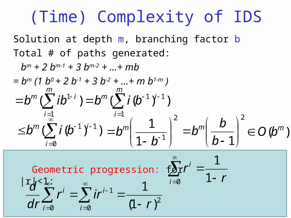
Solution at depth m, branching factor bTotal # of paths generated: bm + 2 bm-1 + 3 bm-2 + ...+ mb = bm (1 b0 + 2 b-1 + 3 b-2 + ...+ m b1-m )
))(()(1
11
1
1
m
i
imm
i
im bibibb
(Time) Complexity of IDS
rr
i
i
1
1
0
Geometric progression: for |r|<1:
)( mbO
20
1
0 )1(
1
rirr
dr
d
i
i
i
i
))((0
11
i
im bib2
11
1
b
bm
2
1
b
bbm
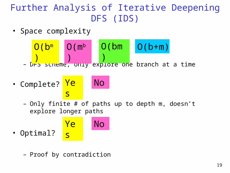
Further Analysis of Iterative Deepening DFS (IDS)
• Space complexity
– DFS scheme, only explore one branch at a time
• Complete?
– Only finite # of paths up to depth m, doesn’t explore longer paths
• Optimal?
– Proof by contradiction
19
O(b+m)O(bm) O(bm)O(mb)
Yes No
Yes No
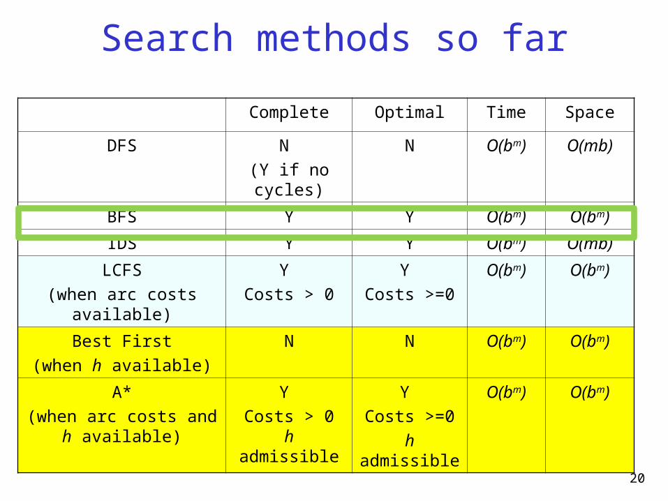
Search methods so far
20
Complete Optimal Time Space
DFS N (Y if no cycles)
N O(bm) O(mb)
BFS Y Y O(bm) O(bm)
IDS Y Y O(bm) O(mb)
LCFS(when arc costs
available)
Y Costs > 0
Y Costs >=0
O(bm) O(bm)
Best First(when h available)
N N O(bm) O(bm)
A*(when arc costs and h
available)
Y Costs > 0
h admissible
Y Costs >=0
h admissible
O(bm) O(bm)
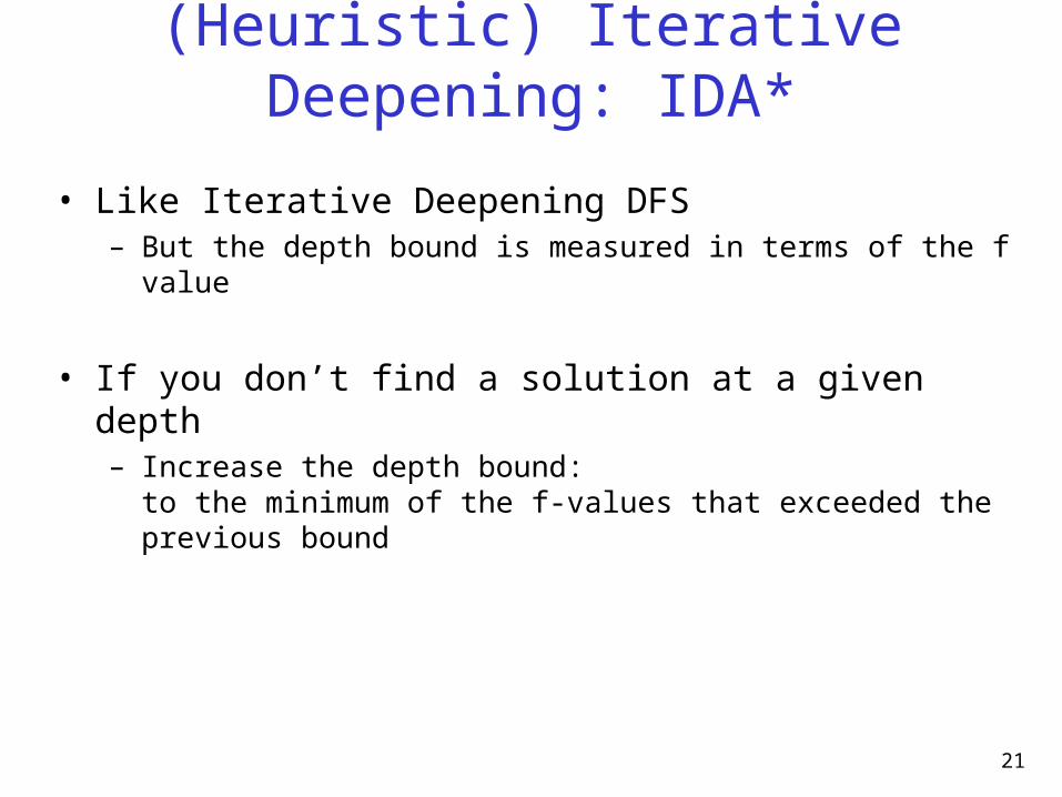
(Heuristic) Iterative Deepening: IDA*
• Like Iterative Deepening DFS– But the depth bound is measured in terms of the f value
• If you don’t find a solution at a given depth– Increase the depth bound:
to the minimum of the f-values that exceeded the previous bound
21
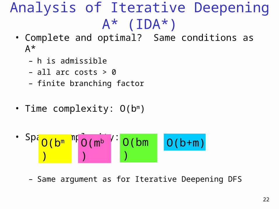
Analysis of Iterative Deepening A* (IDA*)
• Complete and optimal? Same conditions as A*– h is admissible– all arc costs > 0– finite branching factor
• Time complexity: O(bm)
• Space complexity:
– Same argument as for Iterative Deepening DFS
22
O(b+m)O(bm) O(bm)O(mb)
Examples and Clarifications• On the white board …
23
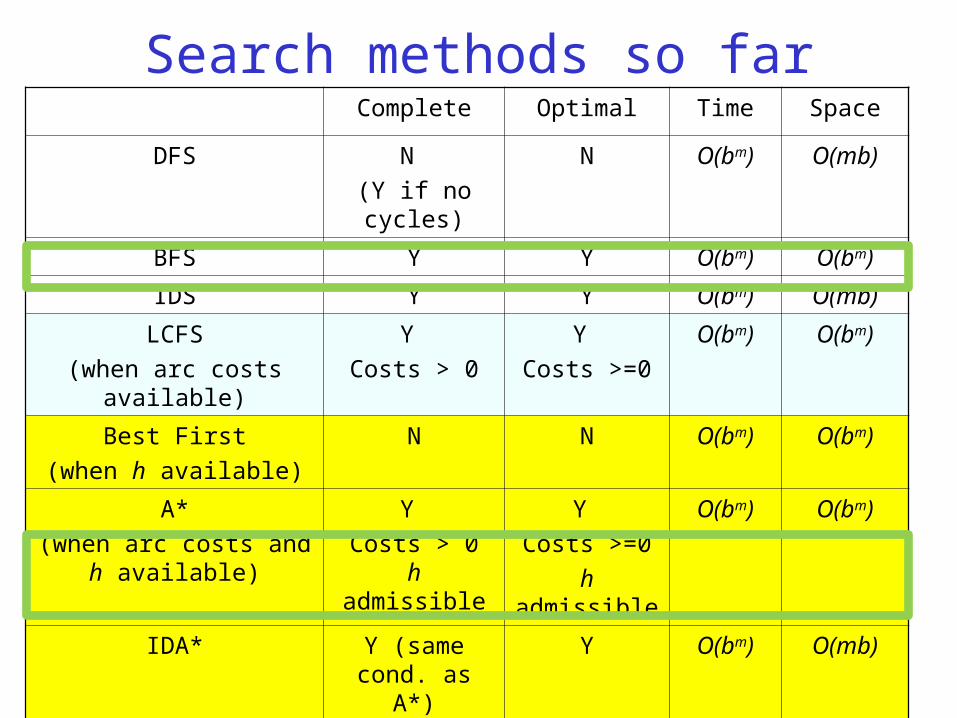
Search methods so farComplete Optimal Time Space
DFS N (Y if no cycles)
N O(bm) O(mb)
BFS Y Y O(bm) O(bm)
IDS Y Y O(bm) O(mb)
LCFS(when arc costs
available)
Y Costs > 0
Y Costs >=0
O(bm) O(bm)
Best First(when h available)
N N O(bm) O(bm)
A*(when arc costs and h
available)
Y Costs > 0
h admissible
Y Costs >=0
h admissible
O(bm) O(bm)
IDA* Y (same cond. as A*)
Y O(bm) O(mb)
Branch & Bound Y (same cond. as A*)
Y O(bm) O(mb)
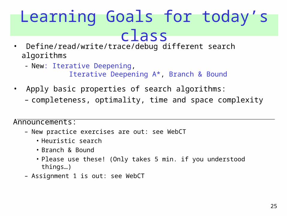
• Define/read/write/trace/debug different search algorithms- New: Iterative Deepening,
Iterative Deepening A*, Branch & Bound
• Apply basic properties of search algorithms: – completeness, optimality, time and space complexity
Announcements: – New practice exercises are out: see WebCT
• Heuristic search• Branch & Bound• Please use these! (Only takes 5 min. if you understood things…)
– Assignment 1 is out: see WebCT
25
Learning Goals for today’s class