Embed Size (px)
Citation preview
Linkoping Studies in Science and TechnologyDissertations, No. 1593
Iterative Methods for Solving the
Cauchy Problem for the Helmholtz
Equation
Lydie Mpinganzima
Department of MathematicsLinkoping University, SE-581 83 Linkoping, Sweden
Linkoping 2014
ii
Iterative Methods for Solving the Cauchy Problem for
the Helmholtz Equation
Copyright c© 2014 Lydie Mpinganzima
Matematiska institutionenLinkopings universitetSE-581 83 Linkoping, [email protected]
Linkoping Studies in Science and TechnologyDissertations, No. 1593
LIU-TEK-LIC-2012:15ISBN 978-91-7519-350-2ISSN 0345-7524
Printed by LiU-Tryck, Linkoping 2014
iii
Abstract
The inverse problem of reconstructing the acoustic, or electromagnetic, field from inex-act measurements on a part of the boundary of a domain is important in applications,for instance for detecting the source of acoustic noise. The governing equation forthe applications we consider is the Helmholtz equation. More precisely, in this thesiswe study the case where Cauchy data is available on a part of the boundary and weseek to recover the solution in the whole domain. The problem is ill-posed in thesense that small errors in the Cauchy data may lead to large errors in the recoveredsolution. Thus special regularization methods that restore the stability with respectto measurements errors are used.
In the thesis, we focus on iterative methods for solving the Cauchy problem.The methods are based on solving a sequence of well-posed boundary value problems.The specific choices for the boundary conditions used are selected in such a way thatthe sequence of solutions converges to the solution for the original Cauchy problem.For the iterative methods to converge, it is important that a certain bilinear form,associated with the boundary value problem, is positive definite. This is sometimesnot the case for problems with a high wave number.
The main focus of our research is to study certain modifications to the prob-lem that restore positive definiteness to the associated bilinear form. First we addan artificial interior boundary inside the domain together with a jump condition thatincludes a parameter µ. We have shown by selecting an appropriate interior boundaryand sufficiently large value for µ, we get a convergent iterative regularization method.We have proved the convergence of this method. This method converges slowly. Wehave therefore developed two conjugate gradient type methods and achieved muchfaster convergence. Finally, we have attempted to reduce the size of the computa-tional domain by solving well–posed problems only in a strip between the outer andinner boundaries. We demonstrate that by alternating between Robin and Dirichletconditions on the interior boundary, we can get a convergent iterative regularizationmethod. Numerical experiments are used to illustrate the performance of the methodssuggested.
Acknowledgements
I take this opportunity to express my gratitude to my supervisors Vladimir Kozlov,Bengt Ove Turesson and Fredrik Berntsson for the guidance, encouragement, patienceand good collaboration. Thanks also to Bjorn Textorius for all the discussions onvarious subjects in mathematics. Thanks to Martin Singull and Johan Thim for Latextemplates, and the Department of Mathematics at Linkoping Universtiy for providinga good working environment.
My studies have been supported by the Swedish International Development Co-operation Agency (Sida) and the University of Rwanda. I am grateful for that.
Linkoping, Mars 31, 2014
Lydie Mpinganzima
iv
Popularvetenskaplig sammanfattning
Det inversa problemet att rekonstruera akustiska eller elektromagnetiska falt i ettomrade fran inexakta matningar pa en del av omradets rand ar viktigt for att t.ex.detektera kallan for akustiskt brus. Sadana problem beskrivs av Helmholtz ekvation.
I avhandlingen studerar vi sadana problem dar Cauchydata ar givna endast paen del av omradets rand och man vill finna losningen i hela omradet. Vi vill alltsalosa Cauchyproblem for Helmholtz ekvation. Sadana problem ar illa stallda, vilketinnebar att sma fel i Cauchydata kan medfora stora fel i losningen. Sarskilda regu-lariseringsmetoder maste darfor anvandas for att ge stabilitet med avseende pa matfel.
Avhandlingens syfte ar att utveckla iterativa losningsmetoder for dessa Cauchy-problem. Metoderna gar ut pa att man loser av en foljd av valstallda randvarde-sproblem for den ursprungliga ekvationen, dar randvillkoren valjs sa att foljden avlosningar konvergerar mot losningen till det ursprungliga Cauchyproblemet. For attde iterativa metoderna skall konvergera ar det viktigt att en viss bilinjar form, somges av randvardesproblemet, ar positivt definit. Detta villkor ar inte alltid uppfylltfor problem med hogt vagtal.
I avhandlingens fokus star darfor studiet av sadana modifieringar av problemetatt den associerade bilinjara formen ar positivt definit. Vi lagger forst till en artificiellinre rand i omradet tillsammans med ett sprangvillkor, som innehaller en parameter µ.Vi visar att man genom att valja den inre randen och parametern lampligt far enkonvergent iterativ regulariseringsmetod. Konvergensen ar langsam, och vi utvecklardarfor i stallet tva metoder av konjugerad gradienttyp, vilka ger mycket snabbarekonvergens.
Slutligen minskar vi berakningsomradets storlek genom att losa de valstalldaproblemen endast i strimman mellan den yttre och den inre randen och visar att mangenom att vaxla mellan Robin och Dirichletvillkor pa den inre randen far en kon-vergent iterativ regulariseringsmetod. Numeriska experiment illustrerar de foreslagnametoderna.
v
List of Papers
The thesis contains three articles and a technical report:
0. F. Berntsson, V.A. Kozlov, L. Mpinganzima, and B.O. Turesson, Numericalsolution for the Cauchy problem for the Helmholtz equation, Technical report,LiTH-MAT-R-2014/04–SE, Department of Mathematics, Linkoping University.
1. F. Berntsson, V.A. Kozlov, L. Mpinganzima, and B.O. Turesson, An alternatingiterative procedure for the Cauchy problem for the Helmholtz equation, InverseProblems in Science and Engineering 22(2014), No. 1, 45–62.
2. F. Berntsson, V.A. Kozlov, L. Mpinganzima, and B.O. Turesson, An acceler-ated alternating iterative procedure for the Cauchy problem for the Helmholtzequation, submitted.
3. F. Berntsson, V.A. Kozlov, L. Mpinganzima, and B.O. Turesson, Robin-Dirichletalgorithms for the Cauchy problem for the Helmholtz equation, manuscript.

vi
vii
Contents
Introduction 1
1 The alternating iterative method 3
2 Summary of papers 4
Paper 0: Numerical solution for the Cauchy problem for the Helmholtz
equation 15
1 Introduction 15
2 An ill–posed operator equation 17
2.1 The operator equation . . . . . . . . . . . . . . . . . . . . . . . . . 172.2 A concrete test problem . . . . . . . . . . . . . . . . . . . . . . . . 18
3 Numerical implementation 20
3.1 The Helmholtz equation in a rectangle . . . . . . . . . . . . . . . . 203.2 The matrix approximation . . . . . . . . . . . . . . . . . . . . . . . 21
4 Numerical study of the Helmholtz equation 22
5 An overview of regularization methods 22
5.1 Direct regularization methods . . . . . . . . . . . . . . . . . . . . . 235.2 Iterative regularization methods . . . . . . . . . . . . . . . . . . . . 26
6 Concluding Remarks 28
Paper 1: An alternating iterative procedure for the Cauchy problem
for the Helmholtz equation 33
1 Introduction 33
1.1 The Helmholtz equation . . . . . . . . . . . . . . . . . . . . . . . . 331.2 The alternating algorithm . . . . . . . . . . . . . . . . . . . . . . . 351.3 Non–convergence of the standard algorithm . . . . . . . . . . . . . 361.4 A modified alternating algorithm . . . . . . . . . . . . . . . . . . . 37
2 Bilinear form and properties of traces 38
2.1 Function spaces . . . . . . . . . . . . . . . . . . . . . . . . . . . . . 382.2 A bilinear form aµ and a sufficient condition for aµ to be positive
definite . . . . . . . . . . . . . . . . . . . . . . . . . . . . . . . . . 392.3 Traces and their properties . . . . . . . . . . . . . . . . . . . . . . 41
3 The main theorem 43
4 Numerical results 46

viii
Paper 2: An accelerated alternating procedure for the Cauchy problem
for the Helmholtz equation 57
1 Introduction 57
1.1 The Helmholtz equation . . . . . . . . . . . . . . . . . . . . . . . . 571.2 The modified alternating algorithm . . . . . . . . . . . . . . . . . . 58
2 Preliminaries 61
2.1 Function spaces . . . . . . . . . . . . . . . . . . . . . . . . . . . . . 612.2 Weak solutions . . . . . . . . . . . . . . . . . . . . . . . . . . . . . 622.3 Inner products . . . . . . . . . . . . . . . . . . . . . . . . . . . . . 63
3 Two operator equations 63
3.1 The first operator equation . . . . . . . . . . . . . . . . . . . . . . 633.2 The second operator equation . . . . . . . . . . . . . . . . . . . . . 653.3 Stopping rule for the modified algorithm . . . . . . . . . . . . . . . 67
4 Conjugate gradient methods 67
4.1 The conjugate gradient method (CGNE) . . . . . . . . . . . . . . . 674.2 Stopping rule for CGNE . . . . . . . . . . . . . . . . . . . . . . . . 684.3 The minimal error method (CGME) . . . . . . . . . . . . . . . . . 694.4 Stopping rule . . . . . . . . . . . . . . . . . . . . . . . . . . . . . . 70
5 Numerical results 71
5.1 Numerical discretization . . . . . . . . . . . . . . . . . . . . . . . . 715.2 Numerical tests . . . . . . . . . . . . . . . . . . . . . . . . . . . . . 735.3 Discussions . . . . . . . . . . . . . . . . . . . . . . . . . . . . . . . 77
6 Conclusions 79
Paper 3: Robin–Dirichlet algorithms for the Cauchy problem for the
Helmholtz equation 87
1 Introduction 87
2 Preliminaries 89
3 Description of the algorithm 89
3.1 The first algorithm . . . . . . . . . . . . . . . . . . . . . . . . . . . 893.2 The second algorithm . . . . . . . . . . . . . . . . . . . . . . . . . 91
4 Sufficient condition for aµ to be positive definite 92
4.1 Example . . . . . . . . . . . . . . . . . . . . . . . . . . . . . . . . . 924.2 Validity of relation (3.4) in a two dimensional case . . . . . . . . . 93
5 Numerical experiments 94
5.1 Finite difference approximation . . . . . . . . . . . . . . . . . . . . 955.2 Numerical tests and discussions . . . . . . . . . . . . . . . . . . . . 97
6 Conclusions 100
1
Introduction
The Helmholtz equation arises in a wide range of applications related to acousticand electromagnetic waves. Depending on the type of the boundary conditions,it is involved in the determination of acoustic cavities [14], the detection of thesource of acoustical noise [17], the description of underwater waves [18], thedetermination of the radiation field surrounding a source of radiation [15], thelocalization of a tumor in a human body [16], the identification and location ofvibratory sources [23], the detection of surface vibrations from interior acousticalpressure [20], etc.
In this paper, we consider the inverse problem of reconstructing the acousticor electromagnetic field from inexact data given only on an open part of theboundary of a given domain. The governing equation for such problem is theHelmholtz equation. This problem is known as the Cauchy problem for theHelmholtz equation and it is ill–posed. According to Hadamard’s definitionof well–posedness, a problem is well–posed if it satisfies the following threerequirements; (see [19]):
1. Existence: There exists a solution of the problem.
2. Uniqueness: There is at most one solution of the problem.
3. Stability: The solution depends continuously on the data.
Any problem that does not possess at least one of these requirements is said tobe ill–posed. However, more attention is usually paid to the third requirement.Indeed, the existence and the uniqueness parts in the Hadamard definition areimportant but if they are not satisfied, they can be enforced by adding addi-tional requirements to the solution or relaxing the notion of a solution. Therequirement that the solution should depend continuously on the data is impor-tant in the sense that if one wants to approximate the solution to a problem,whose solution does not depend continuously on the data by a traditional nu-merical method, then one has to expect that the numerical solution becomesunstable. The computed solution thus has nothing to do with the true solution;see Engl et al. [7].
This definition is made precise with the specification of the function spacesin which the solution is sought and the boundary data are set.
As examples, we consider two Cauchy problems, problems for which theboundary data are given only on a part of the boundary of the domain. Thefirst example is the classical example introduced by Hadamard; see [9]. Thesecond one concerns the main subject of our thesis.
2
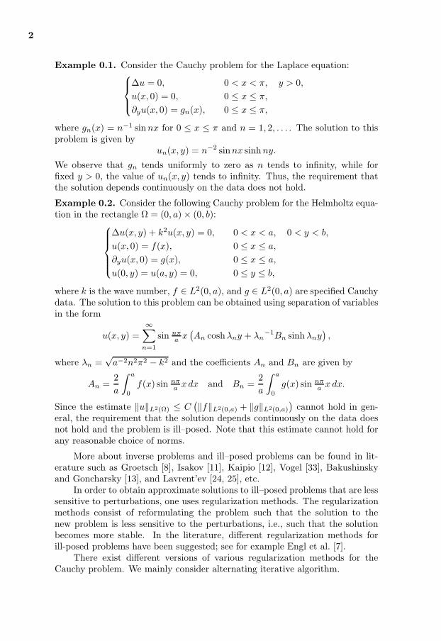
Example 0.1. Consider the Cauchy problem for the Laplace equation:
∆u = 0, 0 < x < π, y > 0,
u(x, 0) = 0, 0 ≤ x ≤ π,
∂yu(x, 0) = gn(x), 0 ≤ x ≤ π,
where gn(x) = n−1 sinnx for 0 ≤ x ≤ π and n = 1, 2, . . . . The solution to thisproblem is given by
un(x, y) = n−2 sinnx sinhny.
We observe that gn tends uniformly to zero as n tends to infinity, while forfixed y > 0, the value of un(x, y) tends to infinity. Thus, the requirement thatthe solution depends continuously on the data does not hold.
Example 0.2. Consider the following Cauchy problem for the Helmholtz equa-tion in the rectangle Ω = (0, a)× (0, b):
∆u(x, y) + k2u(x, y) = 0, 0 < x < a, 0 < y < b,
u(x, 0) = f(x), 0 ≤ x ≤ a,
∂yu(x, 0) = g(x), 0 ≤ x ≤ a,
u(0, y) = u(a, y) = 0, 0 ≤ y ≤ b,
where k is the wave number, f ∈ L2(0, a), and g ∈ L2(0, a) are specified Cauchydata. The solution to this problem can be obtained using separation of variablesin the form
u(x, y) =
∞∑
n=1
sin nπa x
(An coshλny + λn
−1Bn sinhλny),
where λn =√a−2n2π2 − k2 and the coefficients An and Bn are given by
An =2
a
ˆ a
0
f(x) sin nπa x dx and Bn =
2
a
ˆ a
0
g(x) sin nπa x dx.
Since the estimate ‖u‖L2(Ω) ≤ C(‖f‖L2(0,a) + ‖g‖L2(0,a)
)cannot hold in gen-
eral, the requirement that the solution depends continuously on the data doesnot hold and the problem is ill–posed. Note that this estimate cannot hold forany reasonable choice of norms.
More about inverse problems and ill–posed problems can be found in lit-erature such as Groetsch [8], Isakov [11], Kaipio [12], Vogel [33], Bakushinskyand Goncharsky [13], and Lavrent’ev [24, 25], etc.
In order to obtain approximate solutions to ill–posed problems that are lesssensitive to perturbations, one uses regularization methods. The regularizationmethods consist of reformulating the problem such that the solution to thenew problem is less sensitive to the perturbations, i.e., such that the solutionbecomes more stable. In the literature, different regularization methods forill-posed problems have been suggested; see for example Engl et al. [7].
There exist different versions of various regularization methods for theCauchy problem. We mainly consider alternating iterative algorithm.
3
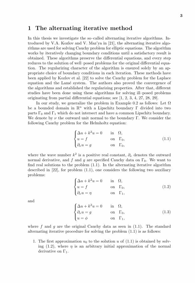
1 The alternating iterative method
In this thesis we investigate the so–called alternating iterative algorithms. In-troduced by V.A. Kozlov and V. Maz’ya in [21], the alternating iterative algo-rithms are used for solving Cauchy problem for elliptic equations. The algorithmworks by iteratively changing boundary conditions until a satisfactory result isobtained. These algorithms preserve the differential equations, and every stepreduces to the solution of well–posed problems for the original differential equa-tion. The regularizing character of the algorithm is ensured solely by an ap-propriate choice of boundary conditions in each iteration. These methods havebeen applied by Kozlov et al. [22] to solve the Cauchy problem for the Laplaceequation and the Lame system. The authors also proved the convergence ofthe algorithms and established the regularizing properties. After that, differentstudies have been done using these algorithms for solving ill–posed problemsoriginating from partial differential equations; see [1, 2, 3, 4, 27, 28, 29].
In our study, we generalize the problem in Example 0.2 as follows: Let Ωbe a bounded domain in R
n with a Lipschitz boundary Γ divided into twoparts Γ0 and Γ1 which do not intersect and have a common Lipschitz boundary.We denote by ν the outward unit normal to the boundary Γ. We consider thefollowing Cauchy problem for the Helmholtz equation:
∆u+ k2u = 0 in Ω,
u = f on Γ0,
∂νu = g on Γ0,
(1.1)
where the wave number k2 is a positive real constant, ∂ν denotes the outwardnormal derivative, and f and g are specified Cauchy data on Γ0. We want tofind real solutions to the problem (1.1). In the alternating iterative algorithmdescribed in [22], for problem (1.1), one considers the following two auxiliaryproblems:
∆u+ k2u = 0 in Ω,
u = f on Γ0,
∂νu = η on Γ1,
(1.2)
and
∆u+ k2u = 0 in Ω,
∂νu = g on Γ0,
u = φ on Γ1,
(1.3)
where f and g are the original Cauchy data as seen in (1.1). The standardalternating iterative procedure for solving the problem (1.1) is as follows:
1. The first approximation u0 to the solution u of (1.1) is obtained by solv-ing (1.2), where η is an arbitrary initial approximation of the normalderivative on Γ1.
4
2. Having constructed u2n, we find u2n+1 by solving (1.3) with φ = u2non Γ1.
3. We then find u2n+2 by solving (1.2) with η = ∂νu2n+1 on Γ1.
Using the problem stated in Example 0.2, we show in Paper 1; see [31], that for
k2 ≥ π2(a−2 + (4b)−2)
this algorithm diverges and it thus cannot be applied for large values of theconstant k2 in the Helmholtz equation. We therefore need to develop appro-priate iterative methods that can be used to solve the Cauchy problem for theHelmholtz equation.
2 Summary of papers
Paper 0
In this paper we study the Cauchy problem for the Helmholtz equation in de-tail. The problem is severely ill-posed and thus challenging to solve numerically.The degree of ill-posedness for a problem is often defined in terms of the singu-lar value decomposition of a linear operator related to the inverse problem wewant to solve. Also, standard numerical methods for solving ill-posed problemsare also often formulated in terms of linear operators, or matrices for discreteproblems. Thus it is often useful to reformulate the Cauchy problem as a linearoperator equation.
Since we are interested in studying the Cauchy problem numerically weselect a concrete test case: Let the domain be Ω=[0, 1]× [0, L] and consider thefollowing well–posed boundary value problem: Find u(x, y) such that
∆u+ k2u = 0, 0 < x < 1, 0 < y < L,uy(x, 0) = 0, 0 < x < 1,u(0, y) = u(1, y) = 0, 0 < y < L,u(x, L) = f(x), 0 < x < 1,
(2.1)
where k2 is the wave number. Using this boundary value problem we define alinear operator
K1 : f(x) 7→ u(x, 0) = g(x). (2.2)
The Cauchy problem for the Helmholtz equation is thus reformulated as a linearoperator equation K1f = g. By discretizing the above mixed boundary valueproblem using finite differences, we approximate the linear operator K1 by amatrix (also denoted by K1) and we are left with a linear system of equations,
K1F = G.
The linear system K1F = G can be analyzed in terms of the singular valuedecomposition. The rate of decay of the singular values determine the degree
5
of ill-posedness of the problem. In the paper we study how the singular valuesdepend on the size of the domain, i.e. the parameter L, and also on the wavenumber k2, and conclude that L significantly influences the stability of theproblem, while the wave number k2 does not.
Further, after having reduced the Cauchy problem to a linear system ofequations, K1F = G, we demonstrate that standard regularization techniques,such as Tikhonov’s method, or the conjugate gradient method, can be used forsolving the problem.
Paper 1
The main idea in this paper is to introduce an artificial interior boundary γ anda positive constant µ. We then assume that
ˆ
Ω
(|∇u|2 − k2u2
)dx+ µ
ˆ
γ
u2 dS > 0, (2.3)
for u ∈ H1(Ω) such that u 6= 0. We denote by [u] and by [∂νu] the jump ofthe function u and the jump of the normal derivative ∂νu across γ, respectively.We propose a modified iterative algorithm that consists of solving the followingboundary value problems alternatively:
∆u+ k2u = 0 in Ω\γ,u = f on Γ0,
∂νu = η on Γ1,
[∂νu] + µu = ξ on γ,
[u] = 0 on γ,
(2.4)
and
∆u+ k2u = 0 in Ω\γ,∂νu = g on Γ0,
u = φ on Γ1,
u = ϕ on γ.
(2.5)
The modified alternating iterative algorithm for solving (1.1) is as follows:
1. The first approximation u0 to the solution of (1.1) is obtained by solv-ing (2.4), where η is an arbitrary initial approximation of the normalderivative on Γ1 and ξ is an arbitrary approximation of [∂νu] + µu on γ.
2. Having constructed u2n, we find u2n+1 by solving (2.5) with φ = u2n on Γ1
and ϕ = u2n on γ.
3. We then obtain u2n+2 by solving the problem (2.4) with η = ∂νu2n+1
on Γ1 and ξ = [∂νu2n+1] + µu2n+1 on γ.
6
In this paper, problems (2.4)–(2.5) are solved in the weak sense. This modifi-cation thus consists of solving two well-posed mixed boundary value problemsfor the original equation. Since the algorithm described through auxiliary prob-lems (2.4) and (2.5) makes sense if (2.3) holds, a sufficient condition concerningthe choice of γ and µ so that (2.3) holds is proved in this paper. It is also shownthat if the positivity condition (2.3) is satified, the sequence (un)
∞n=0 obtained
from this procedure converges in the space H1(Ω) given that the Cauchy data fand g belong to H1/2(Γ0) and H
1/2(Γ0)∗; respectively, and the initial approxi-
mations η and ξ belong to H1/2(Γ1)∗ and ξ ∈ H1/2(γ)∗. In the case of inexact
data, the stopping rule is suggested in Paper 2. This stopping rule is based onthe stopping rule for alternating procedure proposed in [3]. This algorithm thusproduce a stable sequence in the presence of noisy data.
The numerical implementation is based on solving the well-posed boundaryvalue problems (2.4) and (2.5) using the finite difference method. This methodis easy to implemente and during the computations, two matrices together withtheir LU decompositions are also saved which reduces the computation speed.
Paper 2
The convergence of iterative method presented in Paper 1 has been reportedslow. In this paper, we demonstrate how to instead use conjugate gradientmethods for accelerating the convergence. The main requirement for the formu-lation of these methods is the positivity condition (2.3). We thus assume firstthat the interior boundary γ and the constant µ described in Paper 1 are chosenso that the positivity condition (2.3) is satified. We then present two equivalentoperator formulations of problem (1.1). The first formulation corresponds to twoiterations in the modified algorithm and the second to one iteration. The firstone involves the operator B. This operator is defined through the first two iter-ations in the algorithm described in Paper 1. The second one is the operator Nthat is defined from auxiliary problem (2.4). Using auxiliary problem (2.5), wealso find an adjoint operator N∗ to the operator N . We finally prove that thetwo operator equations are identical by showing that N∗N = I −B, where I isthe identity operator.
The convergence results for the conjugate gradient type methods in thecase of exact and inexact Cauchy data proposed by Hanke in [32] are also sug-gested. It is also proved that the modified algorithm presented in Paper 1 canbe interpreted as the Landweber iterative method under some conditions. Fornumerical implementation different choices of the interior boundary have beenalso considered. The numerical results have confirmed that the conjugate gradi-ent methods proposed in this paper accelerate the convergence of the algorithmin Paper 1.
Paper 3
In this paper, we propose two new methods based on iterative procedure sug-gested in [22]. The first algorithm is a slight change of the original method. In
7
Section 1, we present the original algorithm based on solving two well–posedboundary value problems with the Dirichlet and Neumann boundary conditionsiteratively alternated on Γ0 and Γ1. We propose here to instead alternate theDirichlet and Neumann boundary conditions on Γ0 and the Robin and Dirich-let boundary conditions on Γ1. In the same idea, we propose another iterativemethod that consists on introducing first an artificial interior boundary γ in-side Ω and a positive constant µ. In this algorithm, we alternate the Dirichletand Neumann boundary conditions on Γ0 and Γ1 and the Robin and Dirichletboundary conditions on γ.
The first algorithm is described as follows: let us assume that µ is a positiveconstant chosen so that
ˆ
Ω
(|∇u|2 − k2u2
)dx+ µ
ˆ
Γ1
u2 dS > 0, (2.6)
for all u ∈ H1(Ω), such that u 6= 0. Consider now the following boundary valueproblems
∆u+ k2u = 0 in Ω,
u = f on Γ0,
∂νu+ µu = η on Γ1,
(2.7)
and
∆u+ k2u = 0 in Ω,
∂νu = g on Γ0,
u = φ on Γ1.
(2.8)
Assume that f ∈ H1/2(Γ0) and g ∈ H1/2(Γ0)∗ are as in (1.1). The algorithm
for solving (1.1) is described as follows:
1. The first approximation u0 is obtained by solving (2.7), where η is anarbitrary initial approximation of the Robin condition on Γ1.
2. Having constructed u2n, we find u2n+1 by solving (2.8) with φ = u2non Γ1.
3. We then obtain u2n+2 by solving (2.7) with η = ∂νu2n+1 + µu2n+1 on Γ1.
The convergence of this algorithm follows from the convergence of the algorithmin [22]. The main idea in the second algorithm is to introduce an artificialinterior boundary γ and a positive constant µ such that
ˆ
Ω
(|∇u|2 − k2u2
)dx+ µ
ˆ
γ
u2 dS > 0, (2.9)
for all u ∈ H1(Ω), u 6= 0. The new alternating procedure consists of solving the
8
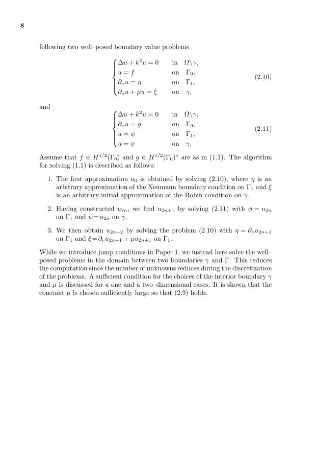
following two well–posed boundary value problems
∆u+ k2u = 0 in Ω\γ,u = f on Γ0,
∂νu = η on Γ1,
∂νu+ µu = ξ on γ,
(2.10)
and
∆u+ k2u = 0 in Ω\γ,∂νu = g on Γ0,
u = φ on Γ1,
u = ψ on γ.
(2.11)
Assume that f ∈ H1/2(Γ0) and g ∈ H1/2(Γ0)∗ are as in (1.1). The algorithm
for solving (1.1) is described as follows:
1. The first approximation u0 is obtained by solving (2.10), where η is anarbitrary approximation of the Neumann boundary condition on Γ1 and ξis an arbitrary initial approximation of the Robin condition on γ.
2. Having constructed u2n, we find u2n+1 by solving (2.11) with φ = u2non Γ1 and ψ=u2n on γ.
3. We then obtain u2n+2 by solving the problem (2.10) with η = ∂νu2n+1
on Γ1 and ξ=∂νu2n+1 + µu2n+1 on Γ1.
While we introduce jump conditions in Paper 1, we instead here solve the well–posed problems in the domain between two boundaries γ and Γ. This reducesthe computation since the number of unknowns reduces during the discretizationof the problems. A sufficient condition for the choices of the interior boundary γand µ is discussed for a one and a two–dimensional cases. It is shown that theconstant µ is chosen sufficiently large so that (2.9) holds.
9
References
[1] S. Avdonin, D. Maxwell, M. Truffer and M. Stuefer, An iterative schemefor determining glacier velocities and stresses, Journal of Glaciology, 54(2008), no. 188, 888–898.
[2] S. Avdonin, V. Kozlov, D. Maxwell and M. Truffer, Iterative methods forsolving a nonlinear boundary inverse problem in glaciology, J. Inv. Ill–PosedProblems, 17 (2009), 239–258.
[3] G. Bastay, T. Johansson, V.A. Kozlov and D. Lesnic,An alternating methodfor the stationary Stokes system, ZAMM, Z. Angew. Math. Mech., 86
(2006), no. 4, 268–280.
[4] R. Chapko and B.T. Johansson, An alternating potential–based approachto the Cauchy problem for the Laplace equation in a planar domain witha cut, Computational Methods in Applied Mathematics, 8 (2008), no. 4,315–335.
[5] D. Colton and R. Kress, Inverse Acoustic and Electromagnetic ScatteringTheory, Second edition, Springer–Verlag, 1998.
[6] A.M. Denisov, Elements of the Theory of Inverse Problems, VSP BV, 1999.
[7] H.W. Engl, M. Hanke and A. Neubauer, Regularization of Inverse Prob-lems, Kluwer Academic Publishers, 2000.
[8] C.W. Groetsch, Inverse Problems in Mathematical Sciences, Vieweg, 1993.
[9] J. Hadamard, Lectures on Cauchy’s Problem in Linear Partial DifferentialEquations, Dover Publications, New York, 1952.
[10] P.C. Hansen, Discrete Inverse Problems: Insight and Algorithms, SIAM,2010.
[11] V. Isakov, Inverse Problems for Partial Differential Equations, Springer–Verlag, 1998.
[12] J. Kaipio and E. Somersalo, Statistical and Computational Inverse Prob-lems, Springer–Verlag, 2005.
[13] A. Bakushinsky and A. Goncharsky, Ill–Posed Problems: Theory and Ap-plications, Kluwer Academic Publishers, 1994.
[14] J.T. Chen and F.C. Wong, Dual formulation of multiple reciprocity methodfor the acoustic mode of a cavity with a thin partition, Journal of Soundand Vibration, 217(1):75–95, 1998.
[15] T. Reginska and K. Reginski, Approximate solution of a Cauchy problemfor the Helmholtz equation, Inverse Problems, 22(3):975–989, 2006.
10
[16] J.D. Shea, P. Kosmas, S.C. Hagness, and B.D. Van Veen, Three–dimensional microwave imaging of realistic numerical breast phantomsvia a multiple frequency inverse scattering technique, Medical Physics,37(8):4210–4226, 2010.
[17] T. Delillo, V. Isakov, N. Valdivia, and L. Wang, The detection of the sourceof acoustical noise in two dimensions, SIAM J. Appl. Math., 61(6):2104–2121, 2001.
[18] G.J. Fix and S.P. Marin, Variational methods for underwater acoustic prob-lems, J. Comput. Phys., 28:253–270, 1978.
[19] A. Kirsch, An Introduction to the Mathematical Theory of Inverse Prob-lems, Springer–Verlag, 1996.
[20] T. Delillo, V. Isakov, N. Valdivia, and L. Wang, The detection of surfacevibrations from interior acoustical pressure, Inverse Problems 19 (2003),507–524
[21] V.A. Kozlov and V.G. Maz’ya, On iterative procedures for solving ill–posed boundary value problems that preserve differential equations, Algebrai Analiz, 192 (1989), 1207–1228.
[22] V.A. Kozlov, V.G. Maz’ya and A.V. Fomin, An iterative method for solvingthe Cauchy problem for elliptic equations, Comput. Maths. Math. Phys.,31 (1991), no. 1, 46–52.
[23] C. Langrenne, M. Melon and A. Garcia, Boundary element method forthe acoustic characterization of a machine in bounded noisy environment,J. Acoust. Soc. Am., 121 (2007), no. 5, 2750–2757.
[24] M.M. Lavrent’ev, V.G. Romanov and S.P. Shishatskii, Ill–Posed Problemsof Mathematical Physics and Analysis, American Mathematical Society,1986.
[25] M.M. Lavrent’ev, Some Improperly Posed Problems of MathematicalPhysics, Springer–Verlag, 1967.
[26] M.M. Lavrent’ev and L.Ya. Savel’ev, Linear Operators and Ill–Posed Prob-lems, Translated form Russian by Nauka Publishers Moscow, 1995.
[27] D. Lesnic, L. Elliot and D.B. Ingham, An alternating boundary elementmethod for solving numerically the Cauchy problems for the Laplace equa-tion, Engineering Analysis with Boundary Elements, 20 (1997), no. 2, 123–133.
[28] D. Lesnic, L. Elliot and D.B. Ingham, An alternating boundary elementmethod for solving Cauchy problems for the biharmonic equation, InverseProblems in Engineering, 5 (1997), no. 2, 145–168.
11
[29] L. Marin, L. Elliott, P.J. Heggs, D.B. Ingham, D. Lesnic and X. Wen, Analternating iterative algorithm for the Cauchy problem associated to theHelmholtz equation, Comput. Math. Appl. Mech. Eng., 192 (2003), 709–722.
[30] M. Hanke, The minimal error conjugate gradient method is a regularizationmethod, Proceedings of the AMS, 123 (1995), no. 11.
[31] F. Berntsson, V.A. Kozlov, L. Mpinganzima, and B.O. Turesson, An alter-nating iterative procedure for the Cauchy problem for the Helmholtz equa-tion, Inverse Problems in Science and Engineering, 22 (2014), no. 1, 45—62.
[32] M. Hanke, Conjugate Gradient Type Methods for Ill–Posed Problems,Longman Scientific and Technical, Harlow, Essex, 1995.
[33] C.R. Vogel, Computational Methods for Inverse Problems, SIAM, 2002.

12

Papers
The articles associated with this thesis have been removed for copyright reasons. For more details about these see: http://urn.kb.se/resolve?urn=urn:nbn:se:liu:diva-105879