iTOUGH2-EOS1sc Users Guide

LBNL-7017E

iTOUGH2-EOS1SC:

Multiphase Reservoir Simulator for Water under

Sub- and Supercritical Conditions

User’s Guide

Lilja Magnúsdóttir Stefan Finsterle

Earth Sciences Division Lawrence Berkeley National Laboratory

Berkeley, CA 94720

October 2015

This work was supported, in part, by the U.S. Dept. of Energy under Contract No. DE-AC02-05CH11231.

iTOUGH2-EOS1SC USER’S GUIDE

DISCLAIMER This document was prepared as an account of work sponsored by the United States Government. While this document is believed to contain correct information, neither the United States Government nor any agency thereof, nor The Regents of the University of California, nor any of their employees, makes any warranty, express or implied, or assumes any legal responsibility for the accuracy, completeness, or usefulness of any information, apparatus, product, or process disclosed, or represents that its use would not infringe privately owned rights. Reference herein to any specific commercial product, process, or service by its trade name, trademark, manufacturer, or otherwise, does not necessarily constitute or imply its endorsement, recommendation, or favoring by the United States Government or any agency thereof, or The Regents of the University of California. The views and opinions of authors expressed herein do not necessarily state or reflect those of the United States Government or any agency thereof or The Regents of the University of California.

Ernest Orlando Lawrence Berkeley National Laboratory is an equal opportunity employer.

iTOUGH2-EOS1SC USER’S GUIDE iii LIST OF FIGURES

TABLE OF CONTENTS 1. INTRODUCTION ......................................................................................................................... 5

2. INSTALLATION AND EXECUTION ........................................................................................ 6

3. THERMODYNAMIC FORMULATION ..................................................................................... 7

4. iTOUGH2-EOS1SC INPUT FORMATS ................................................................................... 11

5. EXAMPLES ................................................................................................................................ 13

5.1 Five-Spot Geothermal Production/Injection under Supercritical Conditions ..................... 13

6. CONCLUDING REMARKS ...................................................................................................... 17

7. ACKNOWLEDGMENT ............................................................................................................. 17

8. REFERENCES ............................................................................................................................ 17

LIST OF FIGURES Figure 1. Regions used in EOS1sc. .................................................................................................. 8Figure 2. Schematic illustration of how the density ρ and internal energy u is calculated outside

the supercritical range based on temperature T and pressure p using IAPWS-95. ........... 9Figure 3. Example of MOMOP block used for the selection of the thermodynamic formulation. ... 11Figure 4. Example of ROCKS block used for specifying depth- or temperature-dependent changes

in permeability and heat capacity. .................................................................................. 12Figure 5. Five-spot injection/production problem showing the element in the middle between the

injector and the producer in gray. ................................................................................... 14Figure 6. TOUGH2-EOS1sc input file (only part of ELEME and CONNE data blocks is shown). 15Figure 7. Pressure-temperature diagram for the element in the middle between the injector and

the producer (shown in gray in Figure 5). ...................................................................... 16

LIST OF TABLES Table 1. Components, phases, and primary variables for EOS1sc. ................................................... 8

Table 2. Start value for density for T>1200°C. ............................................................................... 10

Table 3. Reservoir model parameters. ............................................................................................. 14

iTOUGH2-EOS1SC USER’S GUIDE iv LIST OF FIGURES

PAGE INTENTIONALLY LEFT BLANK

iTOUGH2-EOS1SC USER’S GUIDE PAGE 5 OF 17

1. INTRODUCTION Supercritical fluids exist near magmatic heat sources in geothermal reservoirs, and the high enthalpy fluid is becoming more desirable for energy production with advancing technology. In geothermal modeling, the roots of the geothermal systems are normally avoided but in order to accurately predict the thermal behavior when wells are drilled close to magmatic intrusions, it is necessary to incorporate the heat sources into the modeling scheme. Modeling supercritical conditions poses a variety of challenges due to the large gradients in fluid properties near the critical zone. This work focused on using the iTOUGH2 simulator to model the extreme temperature and pressure conditions in magmatic geothermal systems. The iTOUGH2 simulation-optimization code [Finsterle, 2007a,b,c; http://esd.lbl.gov/iTOUGH2) can be used for history matching, whereby observations reflecting natural state conditions and data obtained during exploitation are analyzed to estimate hydrological and thermal properties as well as other model parameters. iTOUGH2 is based in the TOUGH2 nonisothermal multiphase flow and transport simulator [Pruess et al., 2011; http://esd.lbl.gov/TOUGH2] which has been extensively used to predict the production of fluid mixtures from geothermal reservoirs. However, the standard TOUGH2 module used for such simulations is limited to sub-critical conditions. A new equation-of-state (EOS) module was developed (termed EOS1sc) to extend the operational range of temperature and pressure in iTOUGH2 from 350°C and 100 MPa to 1,000°C and 1,000 MPa and beyond. This manual describes the thermodynamic formulation implemented in iTOUGH2-EOS1SC, and presents examples demonstrating the use of the module.


2. INSTALLATION AND EXECUTION

Compilation and installation of iTOUGH2 is described in Section 5 of Finsterle [2007a] as well as in read-me files distributed with the code. To make an iTOUGH2-EOS1SC executable, the following steps have to be performed:

(1) Adjust maximum array dimensions in file maxsize.inc. A run-time error message will be issued if arrays are insufficiently dimensioned.

(2) Compile file eos1sc.f and link it to the standard iTOUGH2 object files to create the executable. (On Unix platforms, you may use the script it2make [options] 1sc.)

Like any iTOUGH2 application, iTOUGH2-EOS1SC reads in two main input files: an iTOUGH2 and a TOUGH2 input file; options specific to iTOUGH2-EOS1SC are described in Section 4.

iTOUGH2-EOS1SC is executed like any standard iTOUGH2 application, i.e., either using the executable directly, or (preferably) using the script file itough2 (Linux/Unix) or itough2.bat (PC).


3. THERMODYNAMIC FORMULATION EOS1SC is an extension of the EOS1 module for supercritical conditions. In EOS1SC, the IFC-67 thermodynamic formulation given by the International Formulation Committee [1967] and used in EOS1 has been replaced by the IAPWS-IF97 [International Association for the Properties of Water and Steam, 2007] and the IAPWS-95 [International Association for the Properties of Water and Steam, 2002] thermodynamic formulations.

The IAPWS-95 formulation currently serves as the international standard for water’s thermodynamic properties. The operational range for IAPWS-95 has been tested and accepted by the International Association for the Properties of Water and Steam (IAPWS) for up to 1000°C and 100 MPa. The IAPWS-IF97 formulation is a separate, faster formulation based on IAPWS-95, and maintained for industrial use. IAPWS-IF97 is accepted by IAPWS for up to 800°C and 100 MPa, and for up to 2000°C for pressure at or below 50 MPa. Both the IAPWS-95 and IAPWS-IF97 formulations can be extrapolated to extremely high temperatures and densities above the operational limit tested by IAPWS [Magnusdottir and Finsterle, 2015; Yamazaki and Muto, 2004]. Three options to select the thermodynamic formulation are available in EOS1SC: (1) IFC-67, which is only valid for subcritical conditions, (2) IAPWS-IF97, or (3) IAPWS-95 for temperature above or equal to 800°C, and IAPWS-IF97 for temperature below 800°C. For the last option, IAPWS-95 is not used for the whole temperature range because IAPWS-IF97 is significantly faster; IAPWS-IF97 has been accepted by IAPWS to accurately approximate IAPWS-95 within 800°C and 100 MPa.

In the EOS1 module, the primary variables are the same as those of the IFC-67 formulation, i.e. (P, T) for single-phase points, and (Pg, Sg) for two-phase points. In EOS1SC, the primary variables were modified to account for the supercritical region; the same primary variables were used as in the IAPWS-IF97 formulation so that the formulation can be used directly without need for iteration. The IAPWS-IF97 formulation is given in terms of regions nominally defined as liquid, vapor, supercritical, two-phase, and high temperature vapor as shown in Figure 1. Regions 1, 2 and 5 in Figure 1 are individually covered by a fundamental equation for the specific Gibbs free energy given in terms of pressure and temperature. Region 3 is covered by a fundamental equation for the specific Helmholtz free energy and is given in terms of density and temperature. Region 4, i.e., the saturation curve, is given by a saturation-pressure equation. The corresponding primary variables in EOS1SC are (P, T) for the liquid and vapor regions, (Pg, Sg) for the two-phase region, and (ρ, T) for the supercritical region. Thus, the primary variables need to be switched when a region boundary is crossed. An iterative process is used to calculate the thermodynamic variables at the end of every time step and when a region boundary is crossed, the iteration is stopped on a boundary point between the two regions. In EOS1, that boundary point is chosen by projecting the initially calculated new state point vertically onto the boundary to preserve the new temperature. In EOS1SC, an exception has to be made as described by Croucher and O’Sullivan [2008], because the boundary between the liquid and supercritical regions is vertical (see Figure 1). Thus, the boundary point is determined by preserving density for transitions from supercritical to liquid, and by maintaining pressure for transitions from liquid to supercritical. The boundaries of the regions for the IAPWS-IF97 formulation are chosen arbitrarily; they are different from the true phase boundaries. Thus, if the temperature and pressure is above the critical point, the corresponding region in Figure 1 might be vapor with pressure and temperature being used as primary variables, although the true phase is supercritical. The boundary between regions 1 and 3 is at 350°C, the boundary between regions 2 and 5 is at 800°C, and the boundary between regions 2 and 3 is defined by a so-called B23-equation as described by Wagner et al. [2000]. It is not necessary to identify the exact location of the boundaries when using EOS1SC, because the initial conditions can be given in terms of pressure and temperature for all phases. Additionally, the initial conditions can be given in


terms of density and temperature; if the first primary variable is less than 1100, it is assumed to be density. If the IAPWS-IF97 formulation is used above its operational limit, region 5 in Figure 1 is extrapolated. Region 5 can be extrapolated to high temperatures and pressures but extrapolating region 2 gives inaccurate thermodynamic properties [Magnusdottir and Finsterle, 2015]. Table 1 summarizes the components, phases, and primary variable choices for EOS1SC.

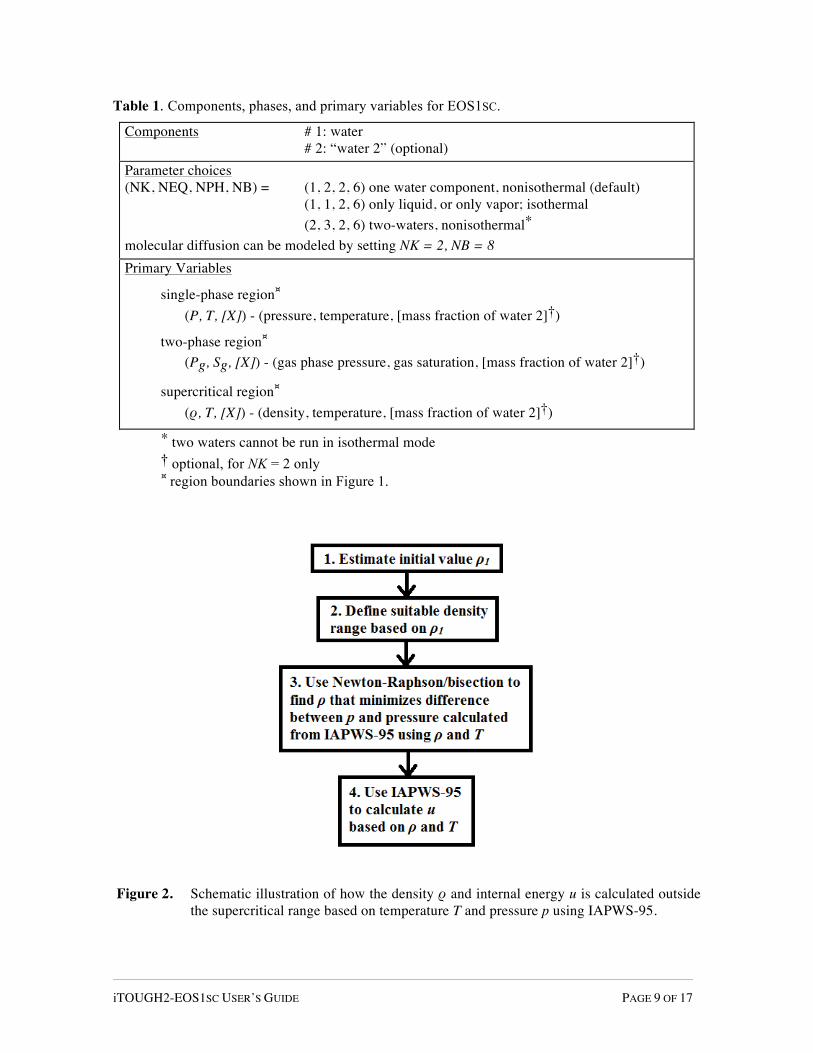
The IAPWS-95 formulation is given by the fundamental equation for the specific Helmholtz free energy. The primary variables are density and temperature for the entire state space. Thus, iterative function inversions are required when using IAPWS-95 outside of the supercritical region in Figure 1. A schematic illustration is provided in Figure 2 of how the density and internal energy are calculated in these regions using IAPWS-95. The function that calculates density, ρ, is used to iteratively evaluate density, because the primary variables of the IAPWS-95 formulation are density and temperature. First, an initial density value, ρ1, is calculated based on temperature and pressure. The IAPWS-IF97 formulation is used to calculate ρ1 if T ≤ 1200°C and the constraints listed in Table 2 are used for T > 1200°C where p1100 is the lower limit of pressure for ρ = 1100 kg/m3 and p800 is the upper limit of pressure for ρ = 800 kg/m3. Then, the lower limit of density is set as 0.8 × ρ1 and the upper limit is set as 1.2 × ρ1. If needed, this range is incrementally increased until the difference between the pressure given and the pressure calculated using IAPWS-95 based on the upper limit of density has an opposite sign to the difference between the pressure given and the pressure calculated based on the lower limit of the density. That way, the root of the function describing the difference between the pressure given and the pressure calculated using IAPWS-95 can be found within the density range using a combination of the Newton-Raphson and bisection methods [Press, 1992] to determine the density corresponding to the pressure given (Step 3 in Figure 2). Once the density has been calculated, the internal energy is calculated based on pressure and density using the IAPWS-95 formulation.

Figure 1. Regions used in EOS1SC.


Table 1. Components, phases, and primary variables for EOS1SC.

Components # 1: water # 2: “water 2” (optional) Parameter choices (NK, NEQ, NPH, NB) = (1, 2, 2, 6) one water component, nonisothermal (default) (1, 1, 2, 6) only liquid, or only vapor; isothermal (2, 3, 2, 6) two-waters, nonisothermal*

molecular diffusion can be modeled by setting NK = 2, NB = 8 Primary Variables

single-phase region¤ (P, T, [X]) - (pressure, temperature, [mass fraction of water 2]†)

two-phase region¤ (Pg, Sg, [X]) - (gas phase pressure, gas saturation, [mass fraction of water 2]†)

supercritical region¤ (ρ, T, [X]) - (density, temperature, [mass fraction of water 2]†)

* two waters cannot be run in isothermal mode † optional, for NK = 2 only ¤ region boundaries shown in Figure 1.

Figure 2. Schematic illustration of how the density ρ and internal energy u is calculated outside

the supercritical range based on temperature T and pressure p using IAPWS-95.


Table 2. Start value for density for T>1200°C.

TOUGH2 bases its calculations on mass and energy balances for each phase; however, there is no phase distinction in the supercritical region. Thus, the saturation line was artificially extended into the supercritical region similarly as described by Croucher and O’Sullivan [2008] for implementing IAPWS-IF97 into AUTOUGH2. Above the extended line the supercritical fluid is theoretically defined ‘liquid’ and below it is called ‘vapor’, although there is no change in physical properties when the line is crossed in the supercritical region. The primary variables in the supercritical region are density and temperature, but in TOUGH2 the first primary variable is assumed to always be pressure. This assumption was removed by making changes to the iTOUGH2 code similar to those described by Talman et al. [2004] for simulating geological CO2 storage.

Constraint Start value for density p > p1100 ρ1 = 1200 kg/m3 pc < p ≤ p1100 ρ1 = 1000 kg/m3 else if steam and… p < 5×104 Pa p > 100×105 Pa 5×104 Pa ≤ p ≤100×105 Pa

ρ1 = 0.1 kg/m3

ρ1 = 100 kg/m3

ρ1 = 1 kg/m3


4. iTOUGH2-EOS1SC INPUT FORMATS

The thermodynamic formulation to be used in EOS1SC are specified in the TOUGH2 input file by defining MOP2(11) in block MOMOP as follows: Record MOMOP

Format (80I1) (MOP2(I),I=1,80)

MOP2(11) Selects thermodynamic formulation

0: IFC-67; for subcritical conditions only

1: IAPWS-IF97

2: IAPWS-IF97 for T<800°C IAPWS-95 for T≥800°C

(Additional MOMOP options are described in the report Enhancements to the TOUGH2 Simulator Implemented in iTOUGH2 [Finsterle, 2015] and in the header of each TOUGH2 output file.)

An example of a MOMOP block invoking a combination of the IAPWS-IF97 and IAPWS-95 formulations is shown in Figure 3.

MOMOP----1----*----2----*----3----*----4----*----5----*----6----*----7----*----8 2

Figure 3. Example of MOMOP block used for the selection of the thermodynamic formulation.


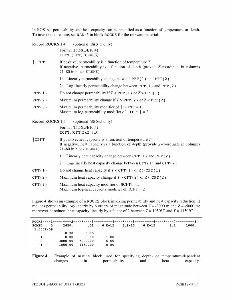
In EOS1sc, permeability and heat capacity can be specified as a function of temperature or depth. To invoke this feature, set NAD=5 in block ROCKS for the relevant material. Record ROCKS.1.4 (optional, NAD=5 only) Format (I5,5X,3E10.4) IPFT, (PFT(I),I=1,3)

|IPFT| If positive, permeability is a function of temperature T If negative, permeability is a function of depth (provide Z-coordinate in columns

71–80 in block ELEME)

1: Linearly permeability change between PFT(1) and PFT(2)

2: Log-linearly permeability change between PFT(1) and PFT(2)

PFT(1) Do not change permeability if T < PFT(1) or Z > PFT(1)

PFT(2) Maximum permeability change if T > PFT(2) or Z < PFT(2)

PFT(3) Maximum permeability modifier of |IPFT| = 1; Maximum log-permeability modifier of |IPFT| = 2 Record ROCKS.1.5 (optional, NAD=5 only) Format (I5,5X,3E10.4) ICFT, (CFT(I),I=1,3)

|IPFT| If positive, heat capacity is a function of temperature T If negative, heat capacity is a function of depth (provide Z-coordinate in columns

71–80 in block ELEME)

1: Linearly heat capacity change between CFT(1) and CFT(2)

2: Log-linearly heat capacity change between CFT(1) and CFT(2)

CFT(1) Do not change heat capacity if T < CFT(1) or Z > CFT(1)

CFT(2) Maximum heat capacity change if T > CFT(2) or Z < CFT(2)

CFT(3) Maximum heat capacity modifier of |ICFT| = 1; Maximum log-heat capacity modifier of |ICFT| = 2

Figure 4 shows an example of a ROCKS block invoking permeability and heat capacity reduction. It reduces permeability log-linearly by 6 orders of magnitude between Z = -3000 m and Z = -5000 m; moreover, it reduces heat capacity linearly by a factor of 2 between T = 1050°C and T = 1150°C.

ROCKS----1----*----2----*----3----*----4----*----5----*----6----*----7----*----8 POMED 5 2650. .01 6.E-15 6.E-15 6.E-15 2.1 1000. 1.000E-09 3 0.30 0.05 1 0.00 0.00 1.00 -2 -3000.00 -5000.00 -6.00 1 1050.00 1150.00 0.50

Figure 4. Example of ROCKS block used for specifying depth- or temperature-dependent changes in permeability and heat capacity.


5. EXAMPLES The examples in this section are all tutorial. Their purpose is to demonstrate the use of iTOUGH2-EOS1SC features.

5.1 Five-Spot Geothermal Production/Injection under Supercritical Conditions The problem presented is a modified version of the geothermal five-spot problem described by Pruess et al. [2012]. The five-spot well pattern shown in Figure 5 has a high degree of symmetry so only one-eighth of the pattern including one injector and one producer is modeled. The reservoir parameters are summarized in Table 3. The reservoir is modeled as a homogeneous porous medium with thickness 305 m, porosity 0.01, and permeability 6 × 10-15 m2. The grain density of the rock is 2650 kg/m3, the specific heat is 1000 J/kg°C, and the heat conductivity is 2.1 W/m°C. EOS1SC can be used to model the extreme temperature and pressure conditions likely to be present at the roots of magmatic geothermal reservoirs. For this case, the initial temperature of the reservoir is set as 1200°C, and the initial pressure is set as 50 MPa. The injection and production rates are 24 kg/s, and the enthalpy of the injected fluid is set as 3000 kJ/kg.

The input file for use with the EOS1SC module is shown in Figure 6. For the first simulation, MOP2(11) is set as 1 so that only the IAPWS-IF97 formulation is used. The cooling of the reservoir is simulated for 55 years of production. Figure 7 shows the pressure-temperature diagram for the element located in the middle between the injector and the producer (element #6, shown in gray in Figure 5). The temperature of the reservoir is initially at 1200ºC and has decreased to 1125°C after 55 years. The temperatures and pressures are always within the operational limit of the IAPWS-IF97 formulation; an extrapolation of the formulation is not required. Next, MOP2(11) is set as 2 so that a combination of the IAPWS-IF97 and IAPWS-95 formulations is used. For this option, IAPWS-95 is used for temperature above or equal to 800°C, and IAPWS-IF97 is used to increase computational speed once the temperature drops below 800°C. In this case, the initial temperature of 1200°C is above the operational temperature limit of 1000°C for IAPWS-95. However, the temperature and pressure results for the element located in the middle between the injector and the producer are identical to when only IAPWS-IF97 is used (see Figure 7). Hence, this extrapolation of the IAPWS-95 formulation above its operational limit gives accurate results.

The main disadvantage of using IAPWS-95 is the relatively slow computational speed. The IAPWS-IF97 formulation is based on IAPWS-95, and it is significantly faster, as discussed by Magnusdottir and Finsterle [2015]. For this case, the CPU time increases by a factor of 10 when using a combination of IAPWS-95 and IAPWS-IF97 instead of using only IAPWS-IF97. This factor would increase for higher simulation temperatures as it depends on how many times the thermodynamic properties are calculated for temperatures above 800°C (i.e. how many times the IAPWS-95 formulation is used during the simulation compared to how many times the IAPWS-IF97 formulation is used). Thus, for faster computational speed it is recommended that IAPWS-IF97 (MOP2(11)=1) is used. For modeling extreme temperatures and pressures above the operational limit of the chosen thermodynamic formulation, it is important to study the accuracy of the extrapolated formulation.


Figure 5. Five-spot injection/production problem showing the element in the middle between the

injector and the producer in gray.

Table 3. Reservoir model parameters.

Formation

Rock grain density 2650 kg/m3 Specific heat 1000 J/kg˚C Heat conductivity 2.1 W/m˚C Porosity 1% Permeability 6.0×10-15 m2 Thickness 305 m Relative permeability: Corey curves irreducible liquid saturation 0.30 irreducible gas saturation 0.05 Initial Conditions Temperature 1200 ˚C Liquid saturation 0.99 Pressure 50 MPa Production/Injection Pattern area 1 km2 Production rate* 24 kg/s

Injection rate* 24 kg/s Injection enthalpy 3000 kJ/kg * Full well basis


sam1sc: Five spot injection/production in supercritical geothermal reservoir ROCKS----1----*----2----*----3----*----4----*----5----*----6----*----7----*----8 POMED 2650. .01 6.E-15 6.E-15 6.E-15 2.1 1000. START----1----*----2----*----3----*----4----*----5----*----6----*----7----*----8 PARAM----1----*-123456789012345678901234----*----5----*----6----*----7----*----8 39999 999910000000000000 4 0 1.736e+9 1.0E05 3.15576E5 1.000e-05 1.000e-01 5.000000000000e+007 1.200000000000e+003 MOMOP----1----*----2----*----3----*----4----*----5----*----6----*----7----*----8 1 RPCAP----1----*----2----*----3----*----4----*----5----*----6----*----7----*----8 3 .30 .05 1 1.0 ELEME----1----*----2----*----3----*----4----*----5----*----6----*----7----*----8 1 POMED0.1906E+060.1250E+04 0. 0.0.1525E+03 2 POMED0.7625E+060.5000E+04 0.7071E+02 0.0.1525E+03 3 POMED0.7625E+060.5000E+04 0.1414E+03 0.0.1525E+03 4 POMED0.7625E+060.5000E+04 0.2121E+03 0.0.1525E+03 5 POMED0.7625E+060.5000E+04 0.2828E+03 0.0.1525E+03 6 POMED0.7625E+060.5000E+04 0.3536E+03 0.0.1525E+03 . ......................... .............................. 30 POMED0.1525E+070.1000E+05 0.3536E+030.2121E+030.1525E+03 31 POMED0.1525E+070.1000E+05 0.4243E+030.2121E+030.1525E+03 32 POMED0.7625E+060.5000E+04 0.4950E+030.2121E+030.1525E+03 33 POMED0.7625E+060.5000E+04 0.2828E+030.2828E+030.1525E+03 34 POMED0.1525E+070.1000E+05 0.3536E+030.2828E+030.1525E+03 35 POMED0.7625E+060.5000E+04 0.4243E+030.2828E+030.1525E+03 36 POMED0.3812E+060.2500E+04 0.3536E+030.3536E+030.1525E+03 CONNE----1----*----2----*----3----*----4----*----5----*----6----*----7----*----8 1 2 10.3536E+020.3536E+020.1078E+05 2 3 10.3536E+020.3536E+020.1078E+05 2 12 20.3536E+020.3536E+020.2157E+05 3 4 10.3536E+020.3536E+020.1078E+05 3 13 20.3536E+020.3536E+020.2157E+05 4 5 10.3536E+020.3536E+020.1078E+05 4 14 20.3536E+020.3536E+020.2157E+05 5 6 10.3536E+020.3536E+020.1078E+05 5 15 20.3536E+020.3536E+020.2157E+05 6 7 10.3536E+020.3536E+020.1078E+05 6 16 20.3536E+020.3536E+020.2157E+05 .. .. ............................... 30 34 20.3536E+020.3536E+020.2157E+05 31 32 10.3536E+020.3536E+020.2157E+05 31 35 20.3536E+020.3536E+020.2157E+05 33 34 10.3536E+020.3536E+020.2157E+05 34 35 10.3536E+020.3536E+020.2157E+05 34 36 20.3536E+020.3536E+020.2157E+05 GENER----1----*----2----*----3----*----4----*----5----*----6----*----7----*----8 1 1 0 MASS 3.00 3.0E6 11 1 0 MASS -3.00 INCON----1----*----2----*----3----*----4----*----5----*----6----*----7----*----8 ENDCY----1----*----2----*----3----*----4----*----5----*----6----*----7----*----8

Figure 6. TOUGH2-EOS1SC input file (only part of ELEME and CONNE data blocks is shown).


Figure 7. Pressure-temperature diagram for the element in the middle between the injector and

the producer (shown in gray in Figure 5).

.


6. CONCLUDING REMARKS The IAPWS-95 and IAPWS-IF97 thermodynamic formulations were added to the iTOUGH2 simulator to extend the applicability of the TOUGH2-based code to temperatures and pressures above 800°C and 100 MPa. Such extreme conditions are likely to occur in magmatic geothermal reservoirs where the heat sources can reach relatively shallow depths. Subcritical conditions and supercritical conditions close to the critical point can be modeled using the thermodynamic formulations IAPWS-IF97, and a combination of IAPWS-95 and IAPWS-IF97. It is recommended that IAPWS-IF97 be used because of its significantly higher computational speed.

7. ACKNOWLEDGMENT We would like to thank Adrian Croucher and Michael O’Sullivan, University of Auckland, New Zealand, for making their AUTOUGH2 code available to us. AUTOUGH2 served as a starting point for the development of EOS1SC. The work of Lilja Magnúsdóttir was funded by the Geothermal Research Group (GEORG), Iceland. Stefan Finsterle was supported, in part, by the U.S. Dept. of Energy under Contract No. DE-AC02-05CH11231.

8. REFERENCES Croucher, A.E., and M.J. O’Sullivan, Application of the computer code TOUGH2 to the simulation

of supercritical conditions in geothermal systems, Geothermics, 37, 662–634, 2008. Finsterle, S., iTOUGH2 User’s Guide, Report LBNL-40040, Lawrence Berkeley National

Laboratory, Berkeley, Calif., 2007a. Finsterle, S., iTOUGH2 Command Reference, Report LBNL-40041 (Updated reprint), Lawrence

Berkeley National Laboratory, Berkeley, Calif., 2007b. Finsterle, S., iTOUGH2 Sample Problems, Report LBNL-40042 (Updated reprint), Lawrence

Berkeley National Laboratory, Berkeley, Calif., 2007c. Finsterle, S., Enhancements to the TOUGH2 Simulator Implemented in iTOUGH2, Report LBNL-

TBD, Lawrence Berkeley National Laboratory, Berkeley, Calif., 2015. IAPWS, Revised release on the IAPWS Industrial Formulation 1997 for the thermodynamic

properties of water and steam, The International Association for the Properties of Water and Steam, Lucerne, Switzerland, 2007.

IAPWS, Release on the IAPWS formulation 2008 for the viscosity of ordinary water substance, The International Association for the Properties of Water and Steam, Berlin, Germany, 2008.

International Formulation Committee of the 6th International Conference on the Properties of Steam, The 1967 IFC Formulation for Industrial Use, Verein Deutscher Ingenieure, Düsseldorf, 1967.

Magnusdottir, L, and Finsterle, S., Extending the applicability of the iTOUGH2 simulator to supercritical conditions, Proceedings, World Geothermal Congress, Melbourne, Australia, 2015.

Pruess, K., C. Oldenburg, and G. Moridis, TOUGH2 User’s Guide, Version 2.1, Report LBNL-43134, Lawrence Berkeley Laboratory, Berkeley, Calif., 2012.

Talman S.J., J.J. Adams, and R.J. Chalaturnyk, Adapting TOUGH2 for general equations of state with application to geological storage of CO2, Comput. Geosci., 20, 543–552, 2004.

Documents

iTOUGH2-EOS1sc Users Guide