Its Imprint on the Cosmic Microwave Background

Initial Condition of the Inflationary Universe and

Its Imprint on the Cosmic Microwave Background

Department of Physics

College of Science

National Taiwan University

Doctoral Dissertation

Yu-Hsiang Lin

Advisor: Pisin Chen, Ph.D.

June 2017

arX

iv:1

710.

1076

3v1

[gr

-qc]

30

Oct

201

7

Acknowledgments

I want to thank Prof. Pisin Chen for bringing me into the field of physics research,

giving me the environment and opportunity to fully dedicate myself into physics.

His support started from the time before I entered the physics department, all the

way to the time I’m leaving. I also have my deepest gratitude to my mother and

my father. You are very successful parents who help your son grow into a man who

can face the challenges in life and pass them. I love you. To my partner and my

guardian, the most beautiful Ting-An: Thank you for sharing the life with me.

I thank Prof. Jiunn-Wei Chen, Prof. Yu-tin Huang, Dr. Dong-han Yeom, and

Dr. Frederico Arroja for being my thesis examination committee and their effort.

I would also like to thank: Dr. Mariam Bouhmadi-Lopez and Yu-Chien Huang for

giving me the opportunity to collaborate; Prof. Keisuke Izumi and Dr. Lance Labun

for their support and many discussions, and being models of good researchers for me;

Dr. Frederico Arroja for his careful reading and thoughtful comments, from which

I benefited a lot; Dr. Dong-han Yeom for working with me and his many interest-

ing ideas; Prof. Teruaki Suyama, Prof. Pei-Ming Ho, Dr. Je-An Gu, Dr. Christo-

pher Gauthier, Dr. Sean Downes, and Dr. Jinn-Ouk Gong, for their discussion and

help; Prof. Jiwoo Nam for his teaching in physics and Korean; Prof. Tom Abel and

Prof. Greg Madejski for having me at the KIPAC family in SLAC; Prof. Leonardo

Senatore, Prof. Stephen Shenker, Prof. Eva Silverstein, and Prof. Andrei Linde for

their discussion at SITP, Stanford University; Prof. Hitoshi Murayama, Prof. Ya-

sunori Nomura, and Dr. Keisuke Harigaya for their help and discussion at Berkeley.

i

Special thanks go to all friends, faculties, and secretaries in LeCosPA, NTU, for

helping me and supporting me all the time. The thesis and related works are in ad-

dition supported by Taiwan Ministry of Science and Technology, as well as Taiwan

National Center for Theoretical Sciences.

It has been a precious and wonderful journey through the ocean of life for me.

Prof. Cha-Ray Chu once said, “Artistic creation is a constant progression. A creator

must cherish her own work; even if it is not perfect, it is what she devoted herself

to.” I am grateful for being lucky to have the opportunity of creating something,

and being able to experience what she said. As American writer Elizabeth Gilbert

put it in her book, Big Magic, “you must stubbornly walk into that room, regardless,

and you must hold your head high. You make it; you get to put it out there. Never

apologize for it, never explain it away, never be ashamed of it. You did your best

with what you knew, and you worked with what you had, in the time that you were

given. You were invited, and you showed up, and you simply cannot do more than

that.” The spirit of the Sand Hill Road days will always be a part of me.

ii

Abstract

There is an apparent power deficit relative to the ΛCDM prediction of the cosmic

microwave background spectrum at large scales, which, though not yet statistically

significant, persists from WMAP to Planck data. It is well-motivated to consider

such power suppression as the imprint of the preinflationary era. The observations

show that about the last 60 e-folds of inflation operates at the energy scale of 1016

GeV. If at the higher energy scales the matter content is in a different phase, or that

the gravity is modified, the evolution of the geometry in the preinflationary universe

may not be the de Sitter expansion in a spatially flat universe, as it is deep in the

inflationary era. In the scenario of “just-enough” inflation, the perturbations at the

largest scales we observe today exit the horizon around the transition time from

preinflation to inflation era, hence carrying the characteristics of the preinflationary

universe. The large-scale spectrum may therefore serve as the window to peek into

the preinflationary universe.

We first present a simple toy model corresponding to a network of frustrated

topological defects of domain walls or cosmic strings that exist previous to the

standard slow-roll inflationary era of the universe. If such a network corresponds

to a network of frustrated domain walls, it produces an earlier inflationary era

that expands more slowly than the standard one does. On the other hand, if the

network corresponds to a network of frustrated cosmic strings, the preinflationary

universe would expand at a constant speed. Those features are phenomenologically

modeled by a Chaplygin gas that can interpolate between a network of frustrated

iii

topological defects and a de Sitter–like or a power-law inflationary era. We show

that these scenarios can alleviate the quadrupole anomaly of the cosmic microwave

background spectrum, based on the approximate initial conditions for the long-

wavelength perturbations. A more thorough and systematic analysis on the initial

vacuum carried out later will show that the preinflationary domain wall dominated

era has a different vacuum state from the approximate one and does not suppress

the long-wavelength spectrum.

We then go further to show that the large-scale spectrum at the end of infla-

tion reflects the super-horizon spectrum of the initial state of the inflaton field. By

studying the curvature perturbations of a scalar field in the Friedmann-Lemaıtre-

Robertson-Walker universe parameterized by the equation of state parameter w, we

find that the large-scale spectrum at the end of inflation reflects the superhorizon

spectrum of the initial state. The large-scale spectrum is suppressed if the universe

begins with the adiabatic vacuum in a superinflation (w < −1) or positive-pressure

(w > 0) era. In the latter case, there is however no causal mechanism to establish

the initial adiabatic vacuum. On the other hand, as long as the universe begins with

the adiabatic vacuum in an era with −1 < w < 0, even if there exists an interme-

diate positive-pressure era, the large-scale spectrum would be enhanced rather than

suppressed. We further calculate the spectrum of a two-stage inflation model with

a two-field potential and show that the result agrees with that obtained from the ad

hoc single-field analysis.

Neither of the two possibilities discovered earlier—the preinflationary superinfla-

tion and positive-pressure eras—that attempt to account for the power suppression

is completely satisfactory as a realistic initial condition of the inflationary universe.

This difficulty may be a hint that the origin of the power suppression does not lie

in the semi-classical physics, but in the quantum theory of gravity. We consider

the Hartle-Hawking no-boundary wave function, which is a solution to the Wheeler-

iv

DeWitt equation, as the initial condition of the universe. We find that the power

suppression can be the consequence of a massive inflaton, whose initial vacuum is

the Euclidean instanton in a compact manifold. We calculate the primordial power

spectrum of the perturbations and show that, as long as the scalar field is moderately

massive, the power spectrum is suppressed at the long-wavelength scales.

Keywords – Cosmic microwave background, large-scale power suppression, topo-

logical defect, domain wall, cosmic string, Chaplygin gas, cosmological perturbation

theory, adiabatic vacuum, inflation, initial condition, spectrum evolution, superin-

flation, two-field inflation, Hartle-Hawking no-boundary wave function, Wheeler-

DeWitt equation, minisuperspace model.

v

vi

Contents

Acknowledgments . . . . . . . . . . . . . . . . . . . . . . . . . . . . . . i

Abstract . . . . . . . . . . . . . . . . . . . . . . . . . . . . . . . . . . . . iii

List of Figures . . . . . . . . . . . . . . . . . . . . . . . . . . . . . . . . viii

List of Tables . . . . . . . . . . . . . . . . . . . . . . . . . . . . . . . . . xv

1 Introduction 1

1.1 Topological Defects . . . . . . . . . . . . . . . . . . . . . . . . . . . . 3

1.2 Relation between initial state and power spectrum . . . . . . . . . . . 5

1.3 Initial Condition from Quantum Cosmology . . . . . . . . . . . . . . 7

2 Preinflationary Network of Frustrated Topological Defects 11

2.1 Model Building and Parameters Fixing . . . . . . . . . . . . . . . . . 13

2.2 Scalar Perturbations . . . . . . . . . . . . . . . . . . . . . . . . . . . 22

3 Power Spectrum in the Universe with Constant Equation of State 31

3.1 Perturbations with Constant Equation of State . . . . . . . . . . . . 32

3.2 Assumption and Character of the Small-Scale Solution . . . . . . . . 36

3.3 Scaling Relation . . . . . . . . . . . . . . . . . . . . . . . . . . . . . . 37

4 Evolution of the Power Spectrum 43

4.1 Slow-Roll . . . . . . . . . . . . . . . . . . . . . . . . . . . . . . . . . 44

4.2 Kinetic—Slow-Roll . . . . . . . . . . . . . . . . . . . . . . . . . . . . 45

4.3 Slow-Roll—Kinetic—Slow-Roll . . . . . . . . . . . . . . . . . . . . . . 50

vii

4.4 Superinflation—Slow-Roll . . . . . . . . . . . . . . . . . . . . . . . . 55

5 Two-field cascade inflation 61

5.1 Background Evolution and the Attractor Solution . . . . . . . . . . . 61

5.2 Perturbations and Initial Conditions . . . . . . . . . . . . . . . . . . 64

5.3 Numerical Solution and the CMB Spectrum . . . . . . . . . . . . . . 67

5.4 Spectrum Evolution Involving a Zero-Pressure Era . . . . . . . . . . . 72

6 No-Boundary Wave Function as the Initial Condition of Inflation 77

6.1 Minisuperspace model . . . . . . . . . . . . . . . . . . . . . . . . . . 78

6.2 Basis functions on the closed universe . . . . . . . . . . . . . . . . . . 81

6.3 Perturbation spectrum from the wave function . . . . . . . . . . . . . 82

6.4 Effect of mass on the power spectrum . . . . . . . . . . . . . . . . . . 86

7 Conclusions and Discussions 97

Bibliography 101

viii

List of Figures

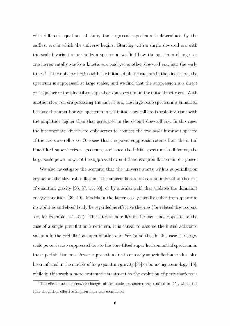
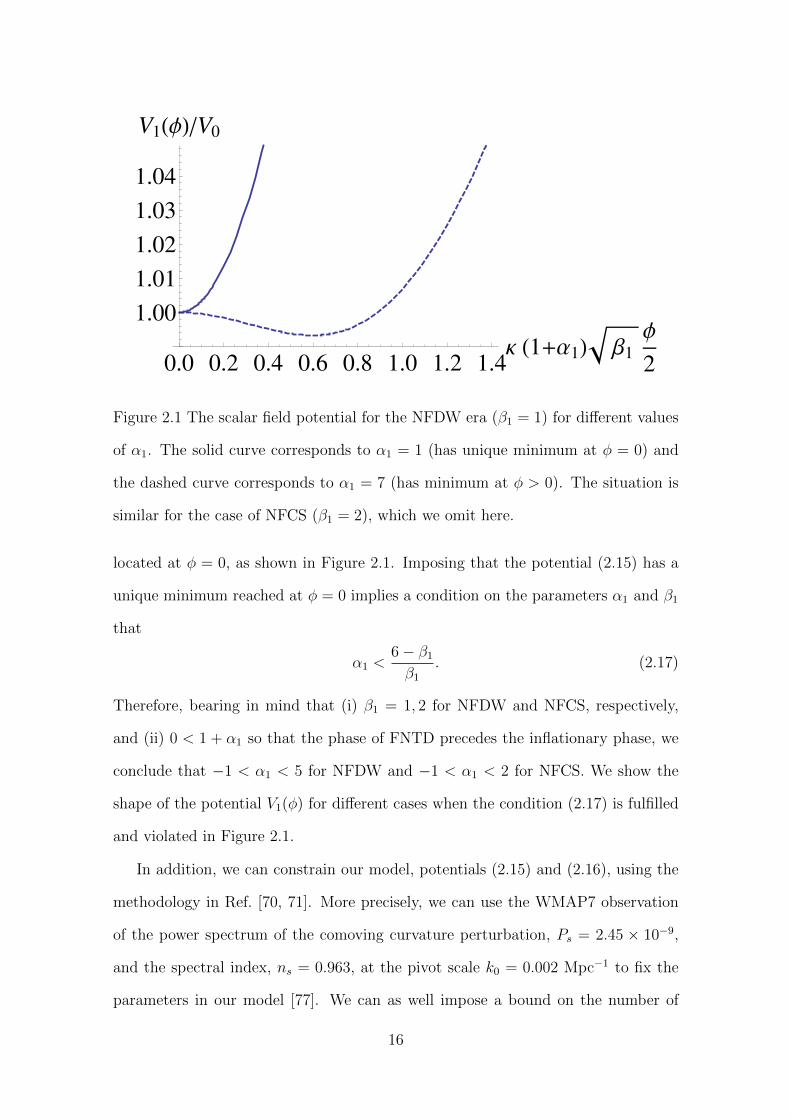
2.1 The scalar field potential for the NFDW era (β1 = 1) for different

values of α1. The solid curve corresponds to α1 = 1 (has unique

minimum at φ = 0) and the dashed curve corresponds to α1 = 7 (has

minimum at φ > 0). The situation is similar for the case of NFCS

(β1 = 2), which we omit here. . . . . . . . . . . . . . . . . . . . . . . 16

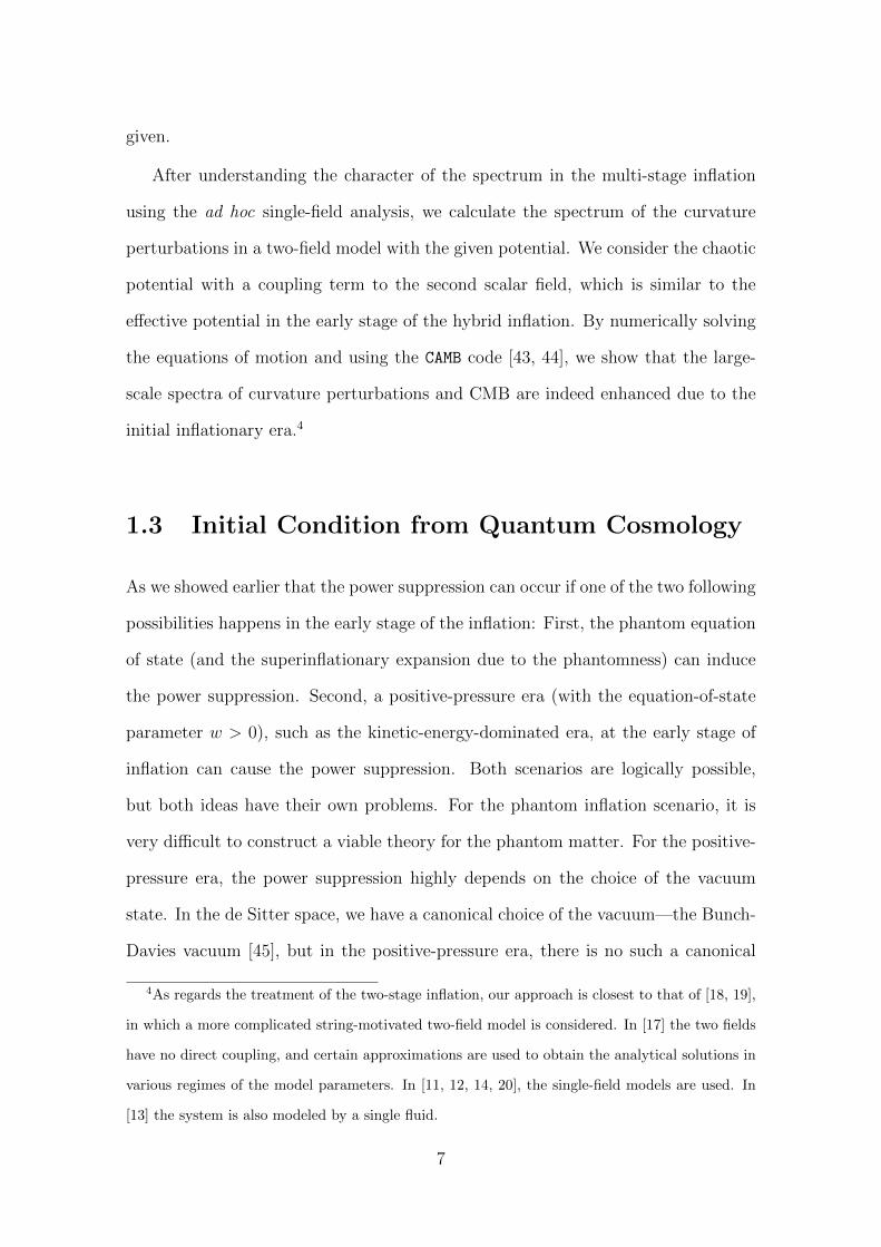
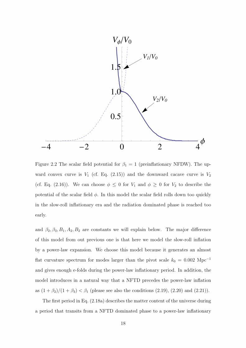
2.2 The scalar field potential for β1 = 1 (preinflationary NFDW). The

upward convex curve is V1 (cf. Eq. (2.15)) and the downward cacave

curve is V2 (cf. Eq. (2.16)). We can choose φ ≤ 0 for V1 and φ ≥ 0

for V2 to describe the potential of the scalar field φ. In this model

the scalar field rolls down too quickly in the slow-roll inflationary era

and the radiation dominated phase is reached too early. . . . . . . . . 18

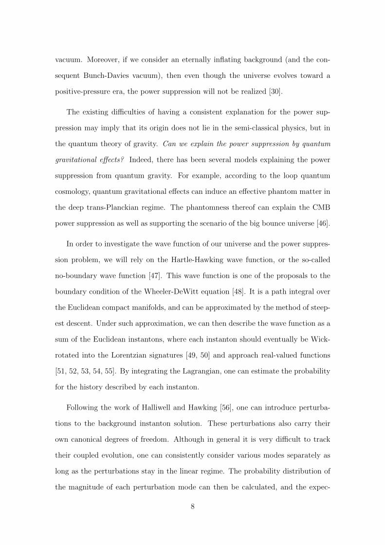
2.3 This plot shows the rescaled potentials given in Eqs. (2.23) and (2.25)

versus the scalar field φ, where V0 = A1/(1+β3)2 (A2/B2)−(1+β2)/(q(1+β3)).

The blue curve corresponds to the NFCS case, and the red curve

corresponds to the NFDW case. The energy scale of inflation, V0, in

our model is about 1015 GeV for both NFDW and NFCS. . . . . . . . 21

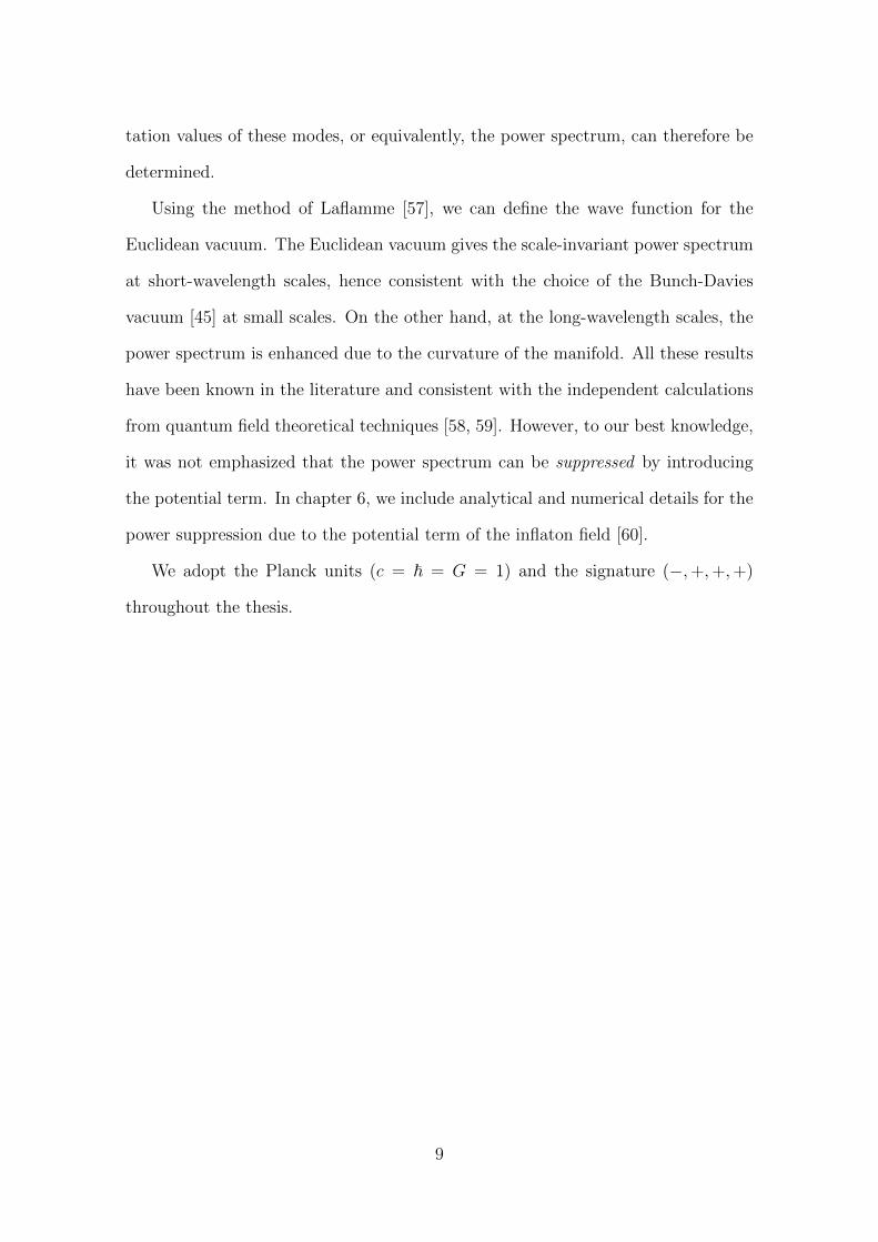
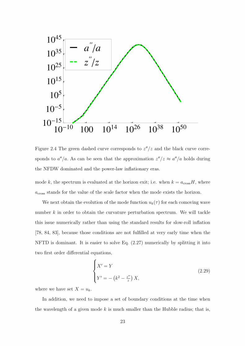
2.4 The green dashed curve corresponds to z′′/z and the black curve cor-

responds to a′′/a. As can be seen that the approximation z′′/z ≈ a′′/a

holds during the NFDW dominated and the power-law inflationary

eras. . . . . . . . . . . . . . . . . . . . . . . . . . . . . . . . . . . . . 23

ix

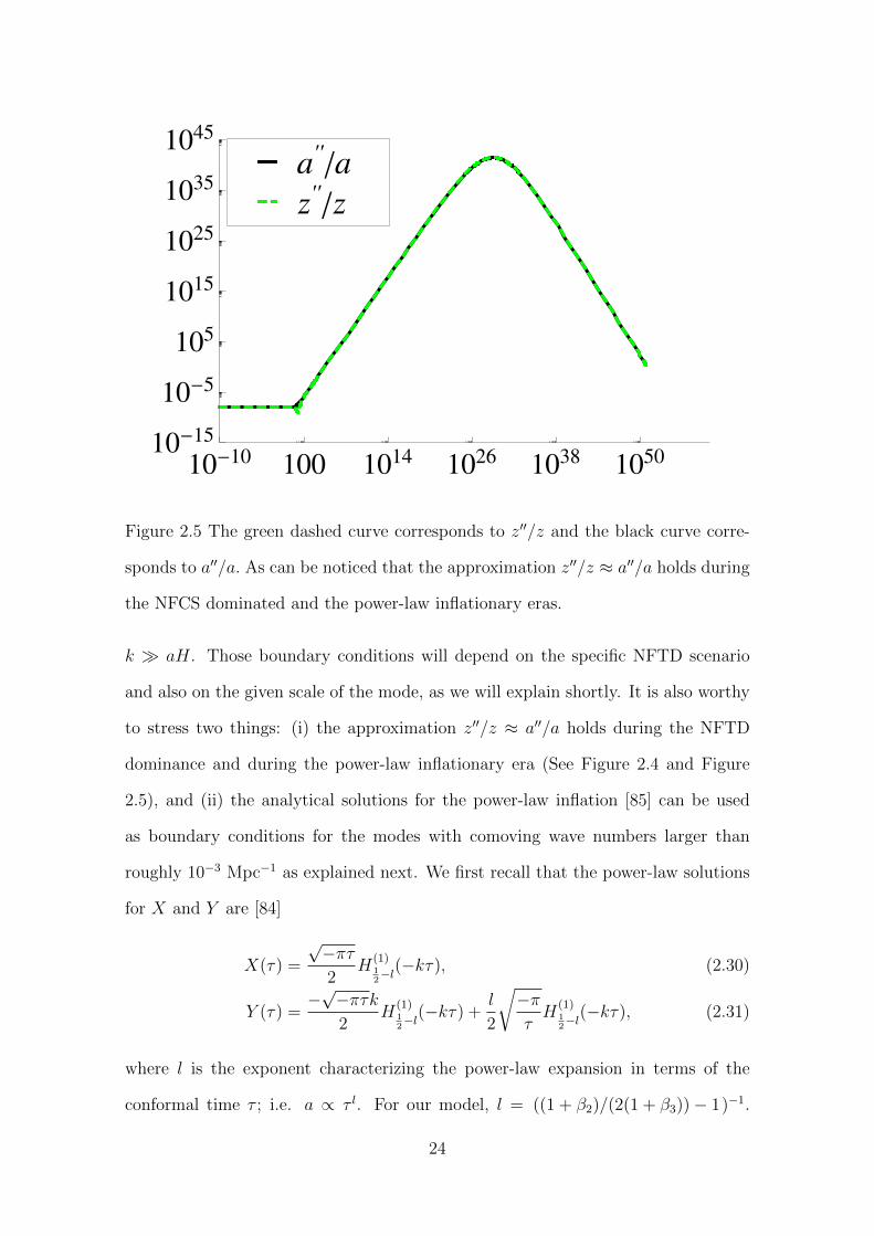
2.5 The green dashed curve corresponds to z′′/z and the black curve cor-

responds to a′′/a. As can be noticed that the approximation z′′/z ≈

a′′/a holds during the NFCS dominated and the power-law inflation-

ary eras. . . . . . . . . . . . . . . . . . . . . . . . . . . . . . . . . . . 24

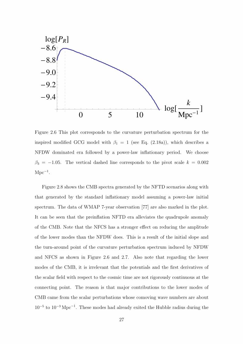
2.6 This plot corresponds to the curvature perturbation spectrum for

the inspired modified GCG model with β1 = 1 (see Eq. (2.18a)),

which describes a NFDW dominated era followed by a power-law

inflationary period. We choose β3 = −1.05. The vertical dashed line

corresponds to the pivot scale k = 0.002 Mpc−1. . . . . . . . . . . . . 27

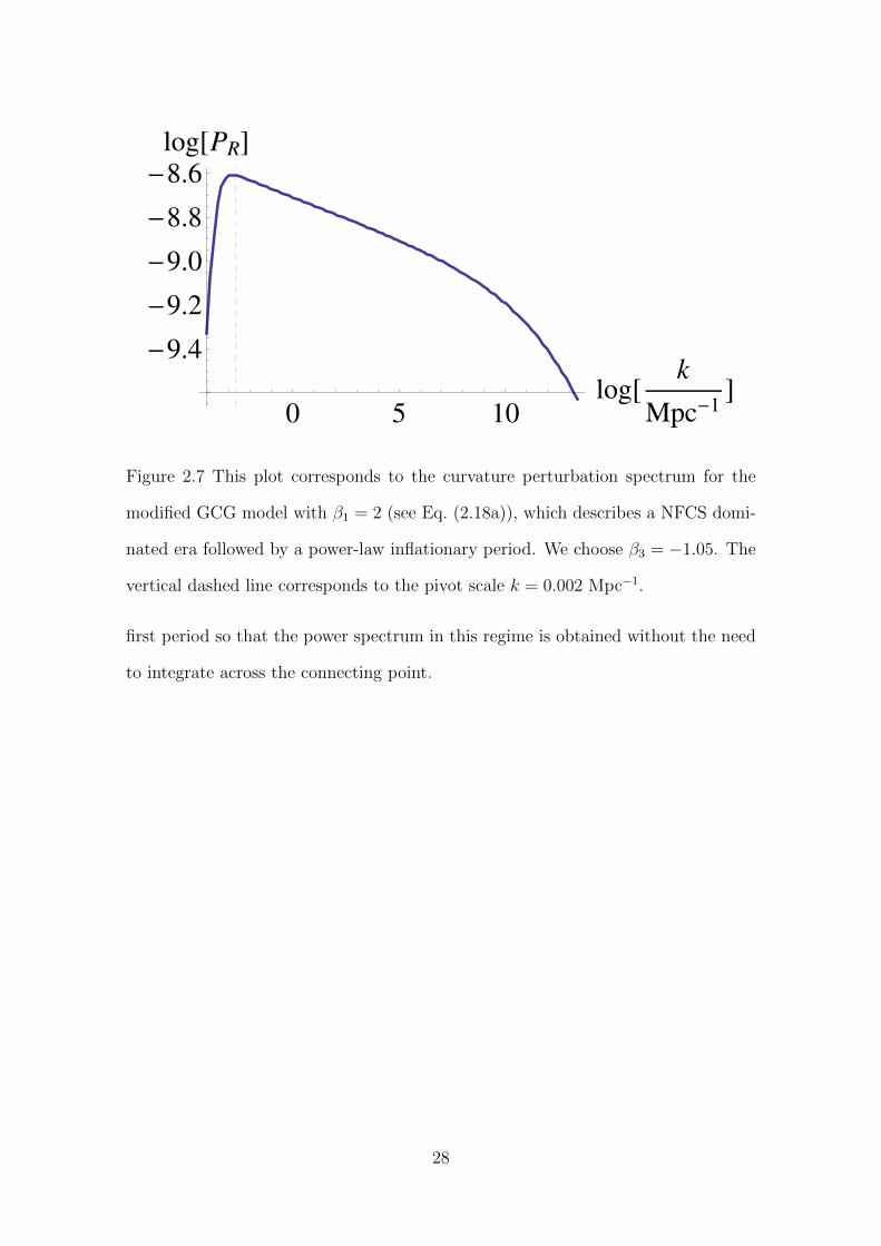
2.7 This plot corresponds to the curvature perturbation spectrum for the

modified GCG model with β1 = 2 (see Eq. (2.18a)), which describes

a NFCS dominated era followed by a power-law inflationary period.

We choose β3 = −1.05. The vertical dashed line corresponds to the

pivot scale k = 0.002 Mpc−1. . . . . . . . . . . . . . . . . . . . . . . . 28

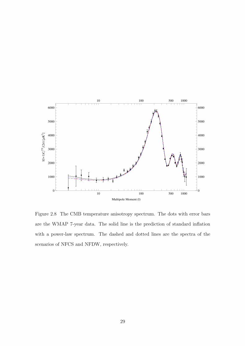
2.8 The CMB temperature anisotropy spectrum. The dots with error

bars are the WMAP 7-year data. The solid line is the prediction

of standard inflation with a power-law spectrum. The dashed and

dotted lines are the spectra of the scenarios of NFCS and NFDW,

respectively. . . . . . . . . . . . . . . . . . . . . . . . . . . . . . . . 29

3.1 The power spectra (3.29) with sample parameters w = −1.2, −2/3,

0, 1/3, 1, 5, and at the slow-roll limit w ' −1. They are plotted

with normalizations such that they have the same magnitude at the

sub-horizon limit. For w ' −1 the power spectrum is given by (3.31),

and the normalization is instead πεP/H2i . The complete relationship

between the slope of the super-horizon spectrum and the equation-

of-state parameter is described by the scaling relation (3.38), and is

plotted in Figure 3.2. . . . . . . . . . . . . . . . . . . . . . . . . . . . 40

x

3.2 The plot of −2µ + 3, the exponent of the power-law scaling relation

(3.38) with respect to the equation-of-state parameter, w. . . . . . . . 41

4.1 Time evolution of the power spectrum in era C in the case of single-

stage evolution (only era C). The solid curves are the spectra of R

from early time to late time (from light to dark). The vertical dashed

lines denote the comoving horizon size at the corresponding instants

(also from light to dark). . . . . . . . . . . . . . . . . . . . . . . . . . 46

4.2 Time evolution of the power spectrum in era B in the case of two-

stage evolution (era B and C). The solid curves are the spectra of R




4.3 Time evolution of the power spectrum in era C in the case of two-

stage evolution (era B and C). The solid curves are the spectra of R




4.4 Illustration of the evolution of the physical wavelengths of the modes

and the Hubble radius with respect to the number of e-fold, N . The

three parallel straight lines denote the modes with three different

wavelengths, long to short from top to bottom (color online). The

corresponding features they generate in the power spectrum, Figure

4.3, are labeled in the legends (top to bottom corresponding to long

to short wavelengths). The black piecewise-connected lines denote

the Hubble radius evolving from the kinetic era to the slow-roll era,

and finally into the ΛCDM era. The shaded region denotes the scales

within which are causally connected. . . . . . . . . . . . . . . . . . . 51

xi

4.5 Time evolution of the power spectrum in era B in the case of three-

stage evolution (era A, B, and C). The solid curves are the spectra

of R from early time to late time (from light to dark). The vertical

dashed lines denote the comoving horizon size at the corresponding

instants (also from light to dark). . . . . . . . . . . . . . . . . . . . . 53

4.6 Time evolution of the power spectrum in era C in the case of three-

stage evolution (era A, B, and C). The solid curves are the spectra

of R from early time to late time (from light to dark). The vertical

dashed lines denote the comoving horizon size at the corresponding

instants (also from light to dark). . . . . . . . . . . . . . . . . . . . . 54

4.7 Illustration of the evolution of the physical wavelengths of the modes

and the Hubble radius with respect to the number of e-fold, N .

The five parallel straight lines denote the modes with different wave-

lengths, long to short from top to bottom (color online). The corre-

sponding features they generate in the power spectrum, Figure 4.6,

are labeled in the legends (top to bottom corresponding to long to

short wavelengths). The black piecewise-connected lines denote the

Hubble radius evolving from the first slow-roll era to the kinetic era,

then to the second slow-roll era, finally into the ΛCDM era. The

shaded region denotes the scales within which are causally connected. 56

4.8 Time evolution of the power spectrum in era S in the case of two-

stage evolution (era S and C), with w = −1.2. The solid curves are

the spectra of R from early time to late time (from light to dark).

The vertical dashed lines denote the comoving horizon size at the

corresponding instants (also from light to dark). . . . . . . . . . . . . 58

xii

4.9 Time evolution of the power spectrum in era C in the case of two-

stage evolution (era S and C), with w = −1.2, NS = 6, and ε = 0.1.

The solid curves are the spectra of R from early time to late time

(from light to dark). The vertical dashed lines denote the comoving

horizon size at the corresponding instants (also from light to dark). . 59

5.1 The spectra of the curvature perturbations with φi = 3.63MP , 3.65MP ,

and 3.67MP . The other parameters are held fixed as λ′ = 10−9,

ψi = 1.60MP , and m = 1.22× 10−6MP . . . . . . . . . . . . . . . . . . 68

5.2 The CMB temperature-temperature correlation (TT) spectra with

φi = 3.63MP , 3.65MP , and 3.67MP . The dots with error bars are the

Planck 2013 data. The other parameters are held fixed as λ′ = 10−9,

ψi = 1.60MP , and m = 1.22× 10−6MP . . . . . . . . . . . . . . . . . . 69

5.3 The CMB TT spectra with ψi = 1.50MP , 1.60MP , and 1.64MP . The

dots with error bars are the Planck 2013 data. The other parameters

are held fixed as λ′ = 10−9, φi = 3.65MP , and m = 1.22× 10−6MP . . 70

5.4 The CMB TT spectra with λ′ = 10−10, 10−9, and 3× 10−9. The dots

with error bars are the Planck 2013 data. The other parameters are

held fixed as φi = 3.65MP , ψi = 1.60MP , and m = 1.22× 10−6MP . . . 71

5.5 Time evolution of the power spectrum in era B in the case of three-

stage evolution (era A, B, and C), in which w = 0 in era B. The solid

curves are the spectra of R from early time to late time (from light

to dark). The vertical dashed lines denote the comoving horizon size

at the corresponding instants (also from light to dark). . . . . . . . . 74

xiii

5.6 Time evolution of the power spectrum in era C in the case of three-

stage evolution (era A, B, and C), in which w = 0 in era B. The solid

curves are the spectra of R from early time to late time (from light

to dark). The vertical dashed lines denote the comoving horizon size

at the corresponding instants (also from light to dark). . . . . . . . . 75

6.1 The power spectrum obtained by numerically solving the perturba-

tions with m = 0, H0 =√

8π/3. . . . . . . . . . . . . . . . . . . . . . 89


tions with m = 1000√

0.1, H0 =√

8π/3. . . . . . . . . . . . . . . . . 89


tions with m =√

0.1×0, 1, . . . , 10, from top to bottom. All spectra

are plotted with H0 =√

8π/3. . . . . . . . . . . . . . . . . . . . . . . 90

6.4 The time evolution of power spectrum in the case of m = 0, H0 =√8π/3. The darker curves correspond to the spectra at later times.

The lightest curve is the initial Lorentzian spectrum at time ti. For

each n mode, the power is evaluated up to its horizon crossing time. . 91

6.5 The time evolution of power spectrum in the case of m = 0.5H0,

H0 =√

8π/3. The darker curves correspond to the spectra at later

times. The lightest curve is the initial Lorentzian spectrum at time

ti. For each n mode, the power is evaluated up to its horizon crossing

time. . . . . . . . . . . . . . . . . . . . . . . . . . . . . . . . . . . . . 92

6.6 The time evolution of power spectrum in the case of m = H0, H0 =√8π/3. The darker curves correspond to the spectra at later times.



xiv

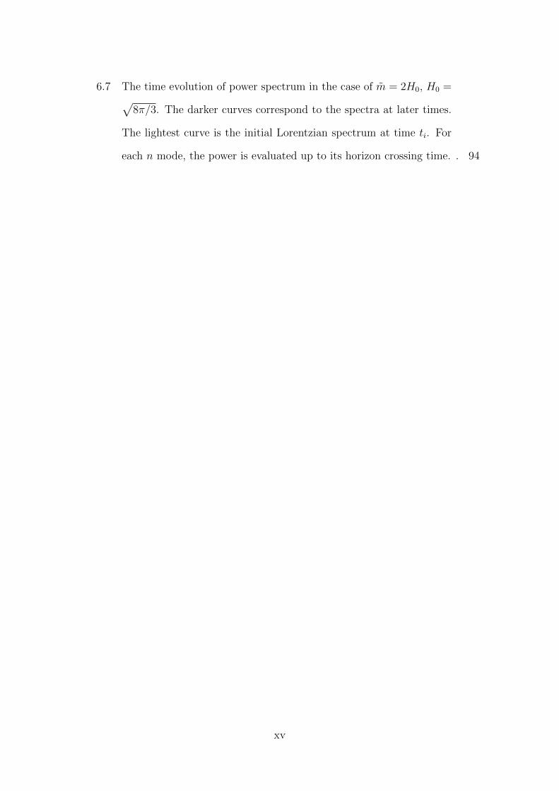
6.7 The time evolution of power spectrum in the case of m = 2H0, H0 =√8π/3. The darker curves correspond to the spectra at later times.



xv

xvi

List of Tables

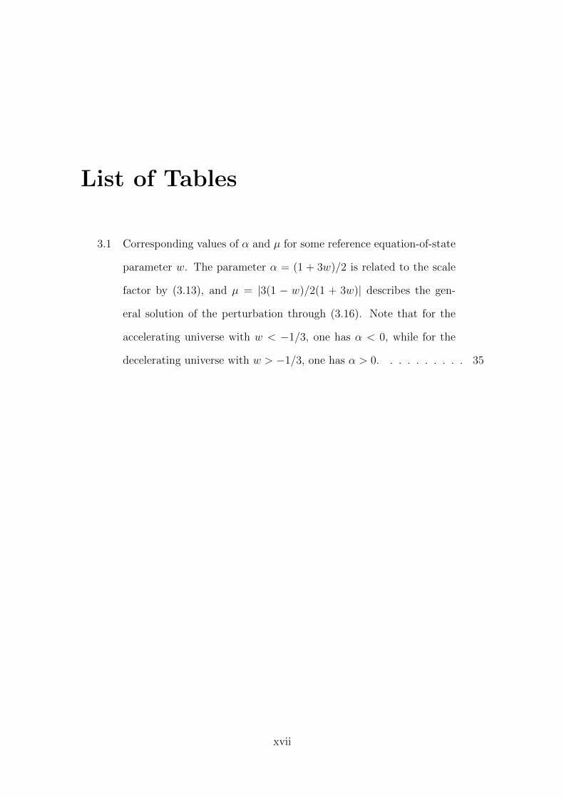
3.1 Corresponding values of α and µ for some reference equation-of-state

parameter w. The parameter α = (1 + 3w)/2 is related to the scale

factor by (3.13), and µ = |3(1 − w)/2(1 + 3w)| describes the gen-

eral solution of the perturbation through (3.16). Note that for the

accelerating universe with w < −1/3, one has α < 0, while for the

decelerating universe with w > −1/3, one has α > 0. . . . . . . . . . 35

xvii

Chapter 1

Introduction

The ΛCDM model of cosmology with an early inflationary era is very successful in

explaining the cosmic microwave background (CMB) power spectrum. However, it

has been observed in the COBE data that the quadrupole power is lower than the

model prediction [1, 2]. This observation is further confirmed by WMAP, reporting

the quadrupole power lower than the theoretical expectation by more than 1σ but

less than 2σ [3]. Although this stand-alone low quadrupole mode may be explained

by the cosmic variance, the Planck observation analyzed the low-` (` < 30) and

high-` (` ≥ 30) spectra separately, and showed that the best-fit amplitude for the

low-` spectrum is 10% lower than that for the high-` one at 2.5–3σ significance

[4, 5].1

The CMB quadruple originates from the lowest modes of the primordial power

spectrum with comoving wave number k of the order of 10−3 Mpc−1. These lowest

modes are the first modes that exit the horizon during inflation and the last ones

that reenter in the radiation, matter, or dark energy dominated eras. Consequently,

we expect that these modes are heavily affected by the physics of the very early

1This low-`/high-` tension is present even when the particularly low quadrupole mode is ex-

cluded from the analysis [4]. In [5] it is further pointed out that the low-` power deficit is mainly

caused by the low multipoles between ` = 20 and 30.

1

universe, possibly the physics prior to the slow-roll inflationary era. Based on this

reasoning, there have been attempts to explain the low-` power suppression of the

CMB by introducing some preinflation era that breaks the slow-roll condition at

about 60 e-folds before the end of inflation [6, 7, 8, 9, 10, 11, 12, 13, 14, 15]. The

basic argument about how an era that deviates from the slow-roll dynamics could

suppress the power is that the amplitude of the curvature perturbation,R ∼ Hδφ/φ,

would decrease as |φ| increases. This scenario is first realized in the single-field

chaotic inflation with potential V = m2φ2/2, where m is the mass of the inflaton. If

the inflaton φ starts with large speed φ2 m2φ2, the kinetic energy dominates the

preinflation universe, and the power at the horizon scale is suppressed [6]. Other

scenarios of violating the slow-roll evolution include the preinflation era filled with

some radiation [7], the primordial black hole remnants [8], or the frustrated network

of topological defects [9]. There are also preinflation models in which the universe

is dominated by the spatial curvature as the emergent property from a number of

moduli fields in the models of solid inflation [16, 10]. All of the models above report

power suppression at the large scales.

On the other hand, the existence of the preinflation decelerating era in models

that predict multi-stage inflation does not always result in power suppression [17,

18, 19, 11, 20, 12, 13, 14]. In the presence of two fields with mass hierarchy, there are

two inflationary eras connected by a decelerating era. With the second inflationary

era identified as the last 60 e-folds of the inflation, it is shown that the power is

enhanced, rather than suppressed, at large scales that cross the horizon during the

first inflationary era or the decelerating era [17]. Similar evolution also occurs in

the early times of the hybrid inflation [21], in which the heavy field is played by the

“waterfall field” who acquires the mass through the coupling to the inflaton field.

In this case, it is however inferred that when the coupling term dominates at the

early times, the inflaton field rolls faster due to the coupling, and eventually leads

2

to the power suppression [6]. Among other models of multi-stage inflation which

commonly have a decelerating era before the last inflationary era, some predict

power suppression at large scales [11, 12, 14], while some predict enhancement [17,

18, 19, 20, 13]. One therefore naturally wonders: What initial condition of inflation

generated by the preinflation era would actually suppress the CMB power spectrum

at large scales?

1.1 Topological Defects

As a toy model to study the preinflation era, we propose a new cosmological pe-

riod just before the slow-roll inflationary era. This period corresponds to an era

described by a network of topological defects, which we will assume to be frustrated

domain walls or cosmic strings [22, 23, 24, 25, 26]. We expect that the production

of topological defects at those scales follows the prediction of high energy physics.

In addition, given that the topological defects era precedes the slow-roll inflation-

ary era, the topological networks will affect mainly the lower modes of the power

spectrum of the scalar and tensorial perturbations. Afterwards, they will soon be

diluted during most of the inflationary era.

Topological defects such as domain walls or cosmic strings can naturally arise in

the history of the universe. In a system that has spontaneous symmetry breaking,

the symmetry that is broken at low temperature is restored at high temperature.

The standard model of the elementary particles has such scenarios including the

electro-weak and GUT (grand unified theory) scale symmetry breaking. In the

early universe, when the temperature is higher than the symmetry breaking scale,

the field is in a global minimum (with quantum fluctuation around the minimum).

As the universe expands, the temperature will eventually drop below the critical

temperature associated with the symmetry. In the low temperature, the potential

of the field has multiple degenerate vacua, and the field will fall down to one of the

3

vacua randomly. Across the space in the universe, there are therefore many spatial

regions in which the field drops to different vacua. Two regions in different vacua are

separated by a domain wall, usually in the case of the discrete symmetry. Cosmic

strings can arise from the breaking of a local U(1) symmetry in the Abelian Higgs

model, which allows the solution of vortex lines [27].

Topological defects are interesting subjects in cosmology for several reasons.

An early one is that it could possibly seed the large-scale structure we observe

today. Planar domain walls, for example, repel the baryonic matter and induce

inhomogeneities [28]. However, if the domain walls are produced too early in the

history of the universe, their energy density may dominate over the other radiation

and baryonic matter sources and significantly alter the observed expansion history.

On the other hand, if the domain walls are created at lower energy scales, while

their energy density will be subdominant, the kinetic energy of them may still spoil

the isotropy of the CMB we observe today.

The network of frustrated domain walls and cosmic strings are considered to

be viable components of the universe because they will not destroy the isotropy of

CMB [29], nor cluster at the small scale [22]. This is because the network structure

makes the domain walls behave like some kind of solid, whose elastic resistance is

only shear deformations. It is hard to have large kinetic movement in orders higher

than the bulk velocity. Moreover, due to their topological nature, the pressure of

such networks of topological defects is negative and of the same order of their energy

density, so their speed of sound is close to the speed of light. As a consequence, their

Jeans length is comparable to the size of the horizon, and they does not collapse at

small scales. One example of the network of domain walls joined by cosmic strings

is given by the complex U(1) scalar field, such as axions [28]. In this type of simple

models the string and anti-directed string will soon annihilate each other within the

Hubble radius, therefore unable to form the stable network structure. To maintain

4

a network structure, one can instead consider, for example, the O(N) field [28],

which has different types of cosmic strings. In this scenario, the probability of pair-

annihilations of the cosmic strings are suppressed because the same type of strings

collide less frequently.

1.2 Relation between initial state and power spec-

trum

One of our most important findings is that, in general, the long-wavelength spectrum

at the end of inflation reflects the super-horizon spectrum of the initial state [30].

To establish such relationship between the initial state and the power spectrum,

we first find the spectrum of the adiabatic vacuum in the universe with a constant

equation of state driven by a scalar field. The conditions of having the blue-tilted,

red-tilted, or scale-invariant spectra at the super-horizon scales are found. The

spectra obtained are based on the assumption that the mode solutions approach the

Minkowski limit at small scales. We point out that in the decelerating universe the

super-horizon modes would enter the horizon and become sub-horizon, which means

that these super-horizon modes are initially causally disconnected. Such assumption

in an initially decelerating universe therefore relies on the final state of the mode

evolution to govern its initial state, which reverses the cause and effect. Later it was

shown that the large-scale power suppression in models with preinflation decelerating

era is actually a consequence of this unnatural yet widely adopted assumption.2

In the next step, we demonstrate that for the universe experiencing several eras

2Such a choice of the initial state for inflation, often referred to as the Bunch-Davies vacuum,

even if there exists a non-slow-roll preinflation phase, has been commonly assumed in the literature

(see, for example, [6, 18, 7, 13, 9, 15, 10]). There also exist numerous proposals of a non-Bunch-

Davies vacuum as the basis of the initial condition for a universe that does not begin with a

slow-roll phase (see, for example, [31, 32, 33, 34]).

5

with different equations of state, the large-scale spectrum is determined by the

earliest era in which the universe begins. Starting with a single slow-roll era with

the scale-invariant super-horizon spectrum, we find how the spectrum changes as

one incrementally stacks a kinetic era, and yet another slow-roll era, into the early

times.3 If the universe begins with the initial adiabatic vacuum in the kinetic era, the

spectrum is suppressed at large scales, and we find that the suppression is a direct

consequence of the blue-tilted super-horizon spectrum in the initial kinetic era. With

another slow-roll era preceding the kinetic era, the large-scale spectrum is enhanced

because the super-horizon spectrum in the initial slow-roll era is scale-invariant with

the amplitude higher than that generated in the second slow-roll era. In this case,

the intermediate kinetic era only serves to connect the two scale-invariant spectra

of the two slow-roll eras. One sees that the power suppression stems from the initial

blue-tilted super-horizon spectrum, and once the initial spectrum is different, the

large-scale power may not be suppressed even if there is a preinflation kinetic phase.

We also investigate the scenario that the universe starts with a superinflation

era before the slow-roll inflation. The superinflation era can be induced in theories

of quantum gravity [36, 37, 15, 38], or by a scalar field that violates the dominant

energy condition [39, 40]. Models in the latter case generally suffer from quantum

instabilities and should only be regarded as effective theories (for related discussions,

see, for example, [41, 42]). The interest here lies in the fact that, opposite to the

case of a single preinflation kinetic era, it is causal to assume the initial adiabatic

vacuum in the preinflation superinflation era. We found that in this case the large-

scale power is also suppressed due to the blue-tilted super-horizon initial spectrum in

the superinflation era. Power suppression due to an early superinflation era has also

been inferred in the models of loop quantum gravity [36] or bouncing cosmology [15],

while in this work a more systematic treatment to the evolution of perturbations is

3The effect due to piecewise changes of the model parameter was studied in [35], where the

time-dependent effective inflaton mass was considered.

6

given.

After understanding the character of the spectrum in the multi-stage inflation

using the ad hoc single-field analysis, we calculate the spectrum of the curvature

perturbations in a two-field model with the given potential. We consider the chaotic

potential with a coupling term to the second scalar field, which is similar to the

effective potential in the early stage of the hybrid inflation. By numerically solving

the equations of motion and using the CAMB code [43, 44], we show that the large-

scale spectra of curvature perturbations and CMB are indeed enhanced due to the

initial inflationary era.4

1.3 Initial Condition from Quantum Cosmology

As we showed earlier that the power suppression can occur if one of the two following

possibilities happens in the early stage of the inflation: First, the phantom equation

of state (and the superinflationary expansion due to the phantomness) can induce

the power suppression. Second, a positive-pressure era (with the equation-of-state

parameter w > 0), such as the kinetic-energy-dominated era, at the early stage of

inflation can cause the power suppression. Both scenarios are logically possible,

but both ideas have their own problems. For the phantom inflation scenario, it is

very difficult to construct a viable theory for the phantom matter. For the positive-

pressure era, the power suppression highly depends on the choice of the vacuum

state. In the de Sitter space, we have a canonical choice of the vacuum—the Bunch-

Davies vacuum [45], but in the positive-pressure era, there is no such a canonical

4As regards the treatment of the two-stage inflation, our approach is closest to that of [18, 19],

in which a more complicated string-motivated two-field model is considered. In [17] the two fields

have no direct coupling, and certain approximations are used to obtain the analytical solutions in

various regimes of the model parameters. In [11, 12, 14, 20], the single-field models are used. In

[13] the system is also modeled by a single fluid.

7

vacuum. Moreover, if we consider an eternally inflating background (and the con-

sequent Bunch-Davies vacuum), then even though the universe evolves toward a

positive-pressure era, the power suppression will not be realized [30].

The existing difficulties of having a consistent explanation for the power sup-

pression may imply that its origin does not lie in the semi-classical physics, but in

the quantum theory of gravity. Can we explain the power suppression by quantum

gravitational effects? Indeed, there has been several models explaining the power

suppression from quantum gravity. For example, according to the loop quantum

cosmology, quantum gravitational effects can induce an effective phantom matter in

the deep trans-Planckian regime. The phantomness thereof can explain the CMB

power suppression as well as supporting the scenario of the big bounce universe [46].

In order to investigate the wave function of our universe and the power suppres-

sion problem, we will rely on the Hartle-Hawking wave function, or the so-called

no-boundary wave function [47]. This wave function is one of the proposals to the

boundary condition of the Wheeler-DeWitt equation [48]. It is a path integral over

the Euclidean compact manifolds, and can be approximated by the method of steep-

est descent. Under such approximation, we can then describe the wave function as a

sum of the Euclidean instantons, where each instanton should eventually be Wick-

rotated into the Lorentzian signatures [49, 50] and approach real-valued functions

[51, 52, 53, 54, 55]. By integrating the Lagrangian, one can estimate the probability

for the history described by each instanton.

Following the work of Halliwell and Hawking [56], one can introduce perturba-

tions to the background instanton solution. These perturbations also carry their

own canonical degrees of freedom. Although in general it is very difficult to track

their coupled evolution, one can consistently consider various modes separately as

long as the perturbations stay in the linear regime. The probability distribution of

the magnitude of each perturbation mode can then be calculated, and the expec-

8

tation values of these modes, or equivalently, the power spectrum, can therefore be

determined.

Using the method of Laflamme [57], we can define the wave function for the

Euclidean vacuum. The Euclidean vacuum gives the scale-invariant power spectrum

at short-wavelength scales, hence consistent with the choice of the Bunch-Davies

vacuum [45] at small scales. On the other hand, at the long-wavelength scales, the

power spectrum is enhanced due to the curvature of the manifold. All these results

have been known in the literature and consistent with the independent calculations

from quantum field theoretical techniques [58, 59]. However, to our best knowledge,

it was not emphasized that the power spectrum can be suppressed by introducing

the potential term. In chapter 6, we include analytical and numerical details for the

power suppression due to the potential term of the inflaton field [60].

We adopt the Planck units (c = ~ = G = 1) and the signature (−,+,+,+)

throughout the thesis.

9

10

Chapter 2

Preinflationary Network of

Frustrated Topological Defects

One natural candidate that may cause the power suppression at the lowest modes of

the CMB spectrum is the primordial topological defect produced during some phase

transition in the preinflationary era. If the universe is populated with the topolog-

ical defects before the slow-roll inflation, the expansion rate of the preinflationary

universe is generally different from that of the de Sitter universe. Therefore, the

curvature perturbations evolves differently in the preinflationary era from the way

they do in the inflationary era. If inflation sustains for just about 60 e-folds, we can

then see the imprint of the transition from the preinflationary to the inflationary

era on the perturbation spectrum.

In this chapter we consider two of the most common types of topological defects—

domain walls and cosmic strings—arising from the phase transitions at the cosmic

scale. To model the transition from the preinflationary to the inflationary era,

we introduce the generalized Chaplygin gas (GCG) [61, 62, 63, 64, 65]. The idea of

describing the early universe by the Chaplygin gas was first suggested in Refs. [66, 67]

(see also [68, 69]) and later extended in Refs. [70, 71, 72, 73, 74, 75]. The energy

density of a network of frustrated topological defects (NFTD) can be described in

11

a compact way, for example, as

ρ =

(B1

aβ1(1+α1)+ A1

)1/(1+α1)

, (2.1)

where a is the scale factor, B1 and A1 are constants related to the energy scale of the

NFTD and the de Sitter-like inflationary era, respectively, α1 and β1 are constants

such that β1 = 1, 2 for the network of frustrated domain walls (NFDW) and the

network of frustrated cosmic strings (NFCS), respectively. We assume that 1 + α1

is positive such that the inflationary era is preceded by a topological dominance

phase. Let us be reminded in this regard that the energy density of NFDW and

NFCS scales as 1/a and 1/a2, respectively [27]. It is worthy to stress that the NFTD

epoch preceding the slow-roll inflationary can in principle produce inflation as well;

indeed this is the case for NFDW, but this inflation is much slower, i.e. much lazier

than the slow-roll inflation. Moreover, for a NFCS dominated period the universe

is increasing its size at a constant speed; i.e. with no acceleration or deceleration.

From now on whenever we refer to a preinflationary era, we will be referring to a

pre-slow-roll inflationary era.

We consider a spatially flat Friedmann-Lemaıtre-Robertson-Walker (FLRW) uni-

verse filled with the matter content described by Eq. (2.1). The energy conservation

gives

ρ+ 3H(ρ+ p) = 0, (2.2)

where a dot corresponds to a derivative with respect to the cosmic time and H

stands for the Hubble rate. By inserting Eq. (2.1) into Eq. (2.2), one obtains the

pressure of the matter content

p =

(β1

3− 1

)ρ− β1

3

A1

ρα1. (2.3)

Note that in terms of the equation of state,

p = wρ, (2.4)

12

where w is the equation-of-state parameter, the universe is in the state of w = −2/3

and w = −1/3 for β = 1 (NFDW dominated) and β = 2 (NFCS dominated),

respectively.

In the Planck unit, the Friedmann equation reads

H2 =κ2

3ρ, (2.5)

where κ2 ≡ 8πG = 8π. The conformal time τ can be expressed as

τ =

√3

κ

b

cA−(b+c)1

(B1

A1

)byc 2F1(c, 1− b, c+ 1, y), (2.6)

where y =[1 + (B1/A1) a−β1(1+α1)

]−1, b = 1 /[β1 (1 + α1)] , c = (−2 + β1)/[2(1 +

α1)β1], and 2F1 is a hypergeometric function [76]. Eq. (2.6) describes that the

universe began in NFTD dominated era in the past infinity, and turned into a de

Sitter-like space, in which a ∝ 1/τ , at later time.

2.1 Model Building and Parameters Fixing

We divide the expansion of the universe into three successive periods: the preinfla-

tionary NFTD dominated era, the slow-roll inflating phase, and the standard ΛCDM

epoch. The energy density of each of these periods can be modeled as

ρ =

[B1

aβ1(1+α1)+ A1

]1/(1+α1)

, (2.7a)[A2 +

B2

a4(1+α2)

]1/(1+α2)

, (2.7b)

ρr0

(a0

a

)4

+ ρm0

(a0

a

)3

+ ρΛ. (2.7c)

Expression (2.7a) describes the energy density of the NFTD era, which was in-

troduced in Eq. (2.1), followed by the de Sitter-like inflating phase. The model

described by Eq. (2.7b) was previously studied within an inflationary framework

in Ref. [70, 71] (see also Ref. [65]) and, under suitable constraints on A2, B2, and

α2, can depict the transition from the de Sitter-like era to the radiation dominated

13

era. The energy density (2.7c) is the standard ΛCDM model, in which ρr0, ρm0,

and ρΛ are the energy densities of the radiation, matter, and dark energy today,

respectively. As we will show later, the parameters of the model can be constrained

using observational data corresponding to the present energy density of radiation,

the scalar power spectrum, and the spectral index at a given pivot scale. In addition,

by requiring that the energy density is continuous at each transition, we have the

conditions

A1 = A(1+α1)/(1+α2)2 , (2.8)

B2 =(ρr0a

40

)1+α2 . (2.9)

In order to obtain the scalar power spectrum, it is useful to model the matter

content in the first two periods of Eq. (2.7); i.e. those described by Eqs. (2.7a)

and (2.7b), through a scalar field, with the condition that the energy density and

pressure of the scalar field are the same as that given by Eqs. (2.7a) and (2.7b). The

energy density and pressure of the scalar field are

ρφ =φ′2

2 a2+ V (φ), pφ =

φ′2

2 a2− V (φ), (2.10)

where the primes denote the derivatives with respect to the conformal time. The

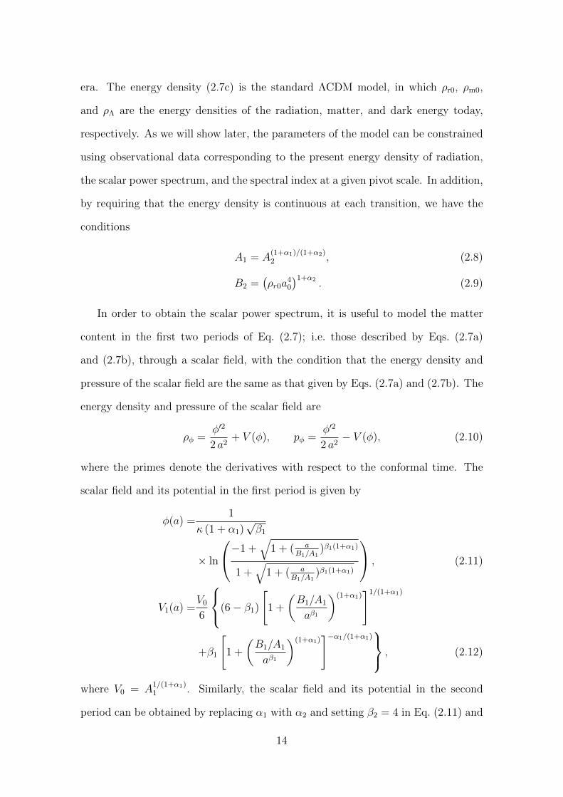
scalar field and its potential in the first period is given by

φ(a) =1

κ (1 + α1)√β1

× ln

−1 +√

1 + ( aB1/A1

)β1(1+α1)

1 +√

1 + ( aB1/A1

)β1(1+α1)

, (2.11)

V1(a) =V0

6

(6− β1)

[1 +

(B1/A1

aβ1

)(1+α1)]1/(1+α1)

+β1

[1 +

(B1/A1

aβ1

)(1+α1)]−α1/(1+α1)

, (2.12)

where V0 = A1/(1+α1)1 . Similarly, the scalar field and its potential in the second

period can be obtained by replacing α1 with α2 and setting β2 = 4 in Eq. (2.11) and

14

Eq. (2.12), giving

φ(a) =1

2κ (1 + α2)

× ln

−1 +√

1 + ( aB2/A2

)4(1+α2)

1 +√

1 + ( aB2/A2

)4(1+α2)

, (2.13)

V2(a) =V0

3

[1 +

(B2/A2

a4

)(1+α2)]

1/(1+α2)

+2

[1 +

(B2/A2

a4

)(1+α2)]−α2/(1+α2)

. (2.14)

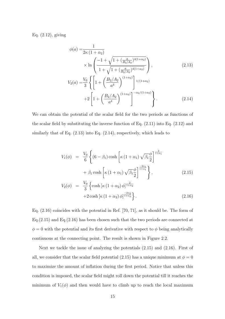
We can obtain the potential of the scalar field for the two periods as functions of

the scalar field by substituting the inverse function of Eq. (2.11) into Eq. (2.12) and

similarly that of Eq. (2.13) into Eq. (2.14), respectively, which leads to

V1(φ) =V0

6

(6− β1) cosh

[κ (1 + α1)

√β1φ

2

] 21+α1

+ β1 cosh

[κ (1 + α1)

√β1φ

2

]−2α11+α1

, (2.15)

V2(φ) =V0

3

cosh [κ (1 + α2)φ]

21+α2

+2 cosh [κ (1 + α2)φ]−2α21+α2

. (2.16)

Eq. (2.16) coincides with the potential in Ref. [70, 71], as it should be. The form of

Eq.(2.15) and Eq.(2.16) has been chosen such that the two periods are connected at

φ = 0 with the potential and its first derivative with respect to φ being analytically

continuous at the connecting point. The result is shown in Figure 2.2.

Next we tackle the issue of analyzing the potentials (2.15) and (2.16). First of

all, we consider that the scalar field potential (2.15) has a unique minimum at φ = 0

to maximize the amount of inflation during the first period. Notice that unless this

condition is imposed, the scalar field might roll down the potential till it reaches the

minimum of V1(φ) and then would have to climb up to reach the local maximum

15

0.0 0.2 0.4 0.6 0.8 1.0 1.2 1.4Κ H1+Α1L Β1

Φ

2

1.00

1.01

1.02

1.03

1.04

V1HΦLV0

Figure 2.1 The scalar field potential for the NFDW era (β1 = 1) for different values

of α1. The solid curve corresponds to α1 = 1 (has unique minimum at φ = 0) and

the dashed curve corresponds to α1 = 7 (has minimum at φ > 0). The situation is

similar for the case of NFCS (β1 = 2), which we omit here.

located at φ = 0, as shown in Figure 2.1. Imposing that the potential (2.15) has a

unique minimum reached at φ = 0 implies a condition on the parameters α1 and β1

that

α1 <6− β1

β1

. (2.17)

Therefore, bearing in mind that (i) β1 = 1, 2 for NFDW and NFCS, respectively,

and (ii) 0 < 1 + α1 so that the phase of FNTD precedes the inflationary phase, we

conclude that −1 < α1 < 5 for NFDW and −1 < α1 < 2 for NFCS. We show the

shape of the potential V1(φ) for different cases when the condition (2.17) is fulfilled

and violated in Figure 2.1.

In addition, we can constrain our model, potentials (2.15) and (2.16), using the

methodology in Ref. [70, 71]. More precisely, we can use the WMAP7 observation

of the power spectrum of the comoving curvature perturbation, Ps = 2.45 × 10−9,

and the spectral index, ns = 0.963, at the pivot scale k0 = 0.002 Mpc−1 to fix the

parameters in our model [77]. We can as well impose a bound on the number of

16

e-folds, Nc, since a given mode exits the horizon until the end of inflation as done in

Ref. [70, 71]. This gives the best-fit values for α2, V0, and, therefore, A2. Notice that

once V0 is fixed, the parameter A1 is fixed for a given α1 as well, since V0 = A1/(1+α1)1 .

The parameter B1 in Eq. (2.7a) fixes the energy density of the NFTD, which

strongly affects the lowest modes that exited the horizon around the onset of infla-

tion, and causes a significant drop on the lowest modes of the primordial spectrum

of the curvature perturbation. Although we expect that the NFTD would affect the

lowest modes, we must make sure that the curvature power spectrum Ps and the

spectral index ns at the pivot scale k0 are consistent with the observations. There-

fore, we choose the value of B1 such that Ps and ns match the observed values at k0,

and that the amplitude of Ps drops at the scales whose comoving wave numbers are

smaller than k0. Roughly speaking, the parameter B1 controls the horizontal shift

of the curvature power spectrum.

However, following this procedure, it turns out that we can not find a set of

values for the parameter B1 that satisfies the constraint on the spectral index. In

fact, in this model B1 turns out to be always smaller than 0.9. This drawback

originates from the second period described by Eq. (2.7b), which corresponds to

the transition from the slow-roll inflationary era to the radiation dominated period.

More precisely, the model described by Eq. (2.7) does not give enough e-folds during

the slow-roll inflationary era. We show, as an example, in Figure 2.2 how the scalar

field rolls too quickly and the radiation dominated phase is reached too early in the

case corresponding to a NFDW.

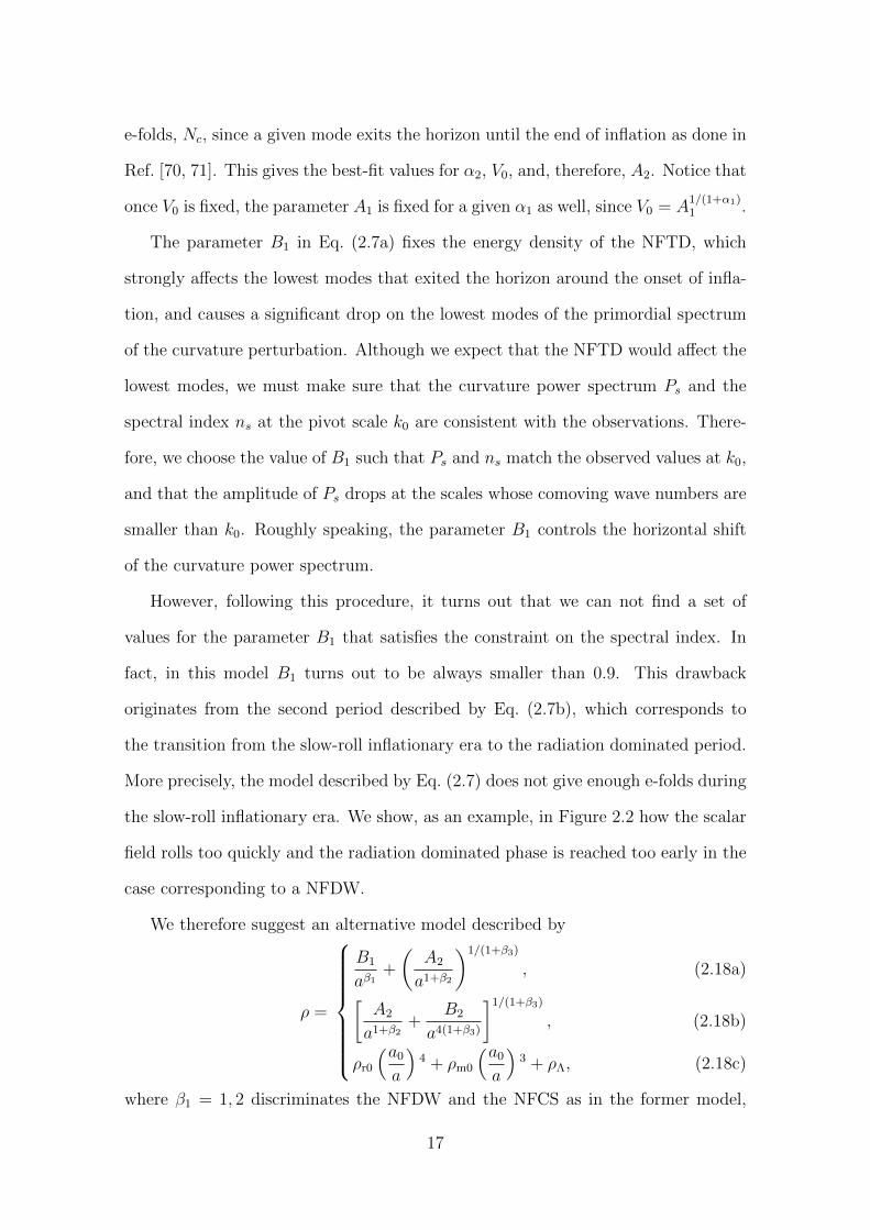
We therefore suggest an alternative model described by

ρ =

B1

aβ1+

(A2

a1+β2

)1/(1+β3)

, (2.18a)[A2

a1+β2+

B2

a4(1+β3)

]1/(1+β3)

, (2.18b)

ρr0

(a0

a

)4 + ρm0

(a0

a

)3 + ρΛ, (2.18c)

where β1 = 1, 2 discriminates the NFDW and the NFCS as in the former model,

17

-4 -2 0 2 4Φ

0.5

1.0

1.5

VΦV0

V1V0

V2V0

Figure 2.2 The scalar field potential for β1 = 1 (preinflationary NFDW). The up-

ward convex curve is V1 (cf. Eq. (2.15)) and the downward cacave curve is V2

(cf. Eq. (2.16)). We can choose φ ≤ 0 for V1 and φ ≥ 0 for V2 to describe the

potential of the scalar field φ. In this model the scalar field rolls down too quickly

in the slow-roll inflationary era and the radiation dominated phase is reached too

early.

and β2, β3, B1, A2, B2 are constants we will explain below. The major difference

of this model from out previous one is that here we model the slow-roll inflation

by a power-law expansion. We choose this model because it generates an almost

flat curvature spectrum for modes larger than the pivot scale k0 = 0.002 Mpc−1

and gives enough e-folds during the power-law inflationary period. In addition, the

model introduces in a natural way that a NFTD precedes the power-law inflation

as (1 + β2)/(1 + β3) < β1 (please see also the conditions (2.19), (2.20) and (2.21)).

The first period in Eq. (2.18a) describes the matter content of the universe during

a period that transits from a NFTD dominated phase to a power-law inflationary

18

era. The parameters B1 and A2 are associated with the energy scale of the NFTD

and that of the power-law inflation, respectively. The second period with the energy

density (2.18b) was previously studied within another inflationary framework in

Ref. [72, 73]. It connects smoothly a power-law inflating phase with a radiation

dominated universe, and the constraints on the parameters β2 and β3 are,1

1 + β2 < 0, (2.19)

1 + β3 < 0, (2.20)

2(1 + β3) < 1 + β2. (2.21)

These constraints imply that (i) there is a power-law inflating phase, (ii) the in-

flationary era precedes the radiation dominated period, and (iii) the null energy

condition is always fulfilled so that there is no superinflationary phase. Finally,

the energy density described by (2.18c) corresponds to the ΛCDM model as that

described by Eq. (2.7c).

Although there seems to be many free parameters, they can be fixed down to

only one by the following procedure: (i) Fix B2 by the current amount of radiation

for a given β3. (ii) Constrain the power-law expansion quantified by A(1+β3)/(1+β2)2

by the WMAP7 data of the curvature power spectrum Ps and the spectral index

ns. Since there are three parameters (A2, β2 and β3) to be constrained by only

two conditions (Ps and ns), we are left with the only one free parameter, which we

choose to be β3. (iii) Fix B1 such that Ps and ns remain the correct values at the

pivot scale k0, and Ps drops only at comoving wave numbers smaller than k0.

Again, it is suitable to introduce a scalar field that mimics the matter content

described in Eqs. (2.18a) and (2.18b); i.e. we describe the dynamics of the model

through a scalar field with a potential whose energy density and pressure can be

obtained from Eq. (2.10). During the NFTD period (cf. Eq. (2.18a)), the mapping

1The notation is different from the one used in the work [72, 73]. The parameters β and α in

Ref. [72, 73] are denoted as β2 and β3 here, respectively.

19

between the scalar field φ and the perfect fluid of our model leads to

φ(a) =√v coth−1

√β1

v

−√β1 tanh−1

√ζ + (1− ζ)

v

β1

, (2.22)

V1(a) =1

6

[(5 +

β3 − β2

1 + β3

)(A2

a1+β2

) 11+β3

+ (6− β1)B1

aβ1

], (2.23)

where ζ = [1 + (A1/(1+β3)2 /B1)aβ1−v]−1, v = (1 + β2)/(1 + β3), and V1(φ) stands for

the scalar field potential during this period. Similarly, we map the perfect fluid with

the energy density (cf. Eq. (2.18b)) to the scalar field φ with a new potential V2(φ)

[72, 73]

φ(a) =1

qκ

[4 tanh−1

√1 +

q

4(1 + β3)

1

1 + ξ− 2

√ζ coth−1

√4

ζ

(1 +

q

4(1 + β3)

1

1 + ξ

)],

(2.24)

V2(a) = A1/(1+β3)2

(A2

B2

)−ζ/q(1 + ξ)1/(1+β3)

ξ−ζ/q(

1

3− q

6(1 + β3)

1

1 + ξ

),

(2.25)

where ξ = (B2/A2)aq and q = 1+β2−4(1+β3). The potential (2.25) was previously

obtained in Ref. [72, 73]. Such a potential, with an appropriate initial condition,

drives a power-law inflation and mimics a radiation dominated universe afterwards.

Unlike the previous model described by Eq. (2.11)-(2.12) and Eq. (2.13)-(2.14),

here it is not feasible to find analytically the inverse functions of Eq. (2.22) and

Eq. (2.24), so we cannot obtain the analytical forms of the potential as functions

of φ. We thus connect the scalar field potential numerically. V1(a) and V2(a) are

connected at the intersection of the first two periods (Eq. (2.18a) and Eq. (2.18b)),

20

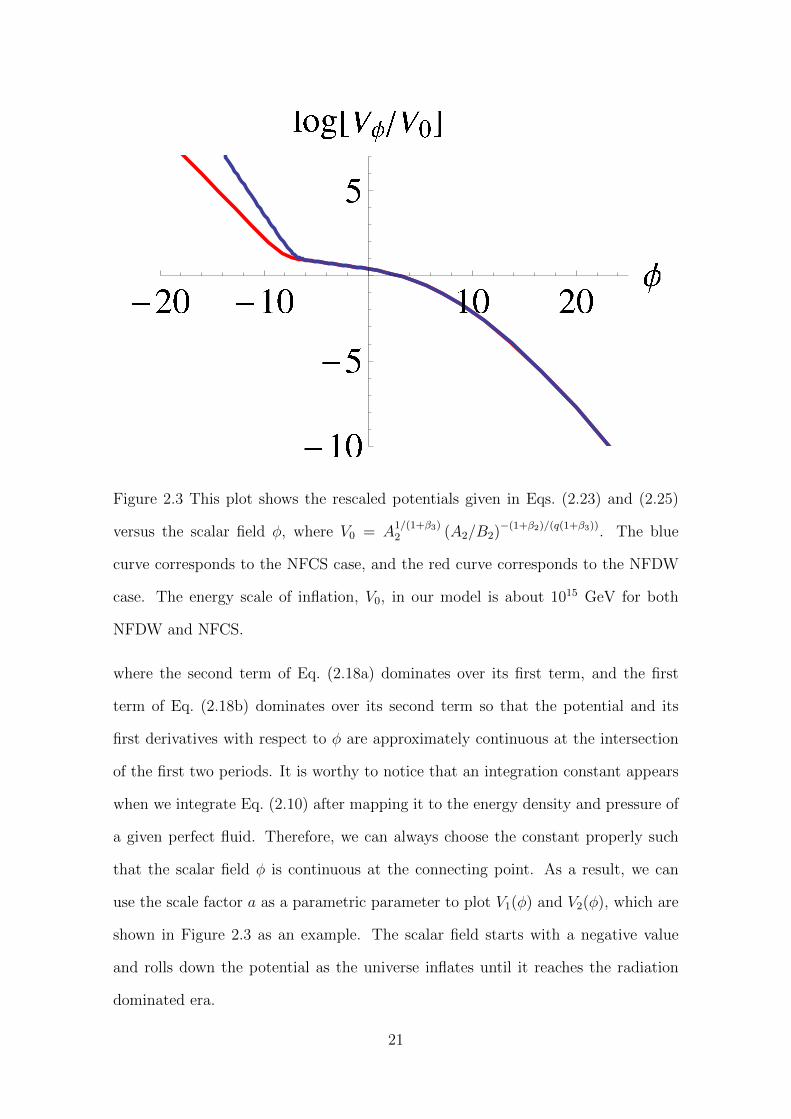
Figure 2.3 This plot shows the rescaled potentials given in Eqs. (2.23) and (2.25)

versus the scalar field φ, where V0 = A1/(1+β3)2 (A2/B2)−(1+β2)/(q(1+β3)). The blue

curve corresponds to the NFCS case, and the red curve corresponds to the NFDW

case. The energy scale of inflation, V0, in our model is about 1015 GeV for both

NFDW and NFCS.

where the second term of Eq. (2.18a) dominates over its first term, and the first

term of Eq. (2.18b) dominates over its second term so that the potential and its

first derivatives with respect to φ are approximately continuous at the intersection

of the first two periods. It is worthy to notice that an integration constant appears

when we integrate Eq. (2.10) after mapping it to the energy density and pressure of

a given perfect fluid. Therefore, we can always choose the constant properly such

that the scalar field φ is continuous at the connecting point. As a result, we can

use the scale factor a as a parametric parameter to plot V1(φ) and V2(φ), which are

shown in Figure 2.3 as an example. The scalar field starts with a negative value

and rolls down the potential as the universe inflates until it reaches the radiation

dominated era.

21

2.2 Scalar Perturbations

The accelerated expansion of the universe during the primordial inflationary era con-

verts the initial quantum fluctuations in the universe into macroscopic cosmological

perturbations, which leads to the inhomogeneity we observe nowadays in the CMB

[78, 79]. Following the standard approach, we will use gauge invariant quantities

that involve the metric perturbations and the scalar field fluctuations [80]. For con-

venience, we will choose the comoving curvature perturbation, R, which in addition

is conserved on large scales [81, 82].

We expect that a NFTD in the very early universe and just before the infla-

tionary era could give the appropriate corrections to the quadrupole modes of the

CMB data as observed nowadays [77]. We will next quantify the quantum cosmolog-

ical perturbations during that period and obtain the power spectrum of the scalar

perturbations.

The scalar perturbations can be described by introducing the variable (see, for

example, Ref. [83])

u = zR, (2.26)

where z ≡ aφH

. The variable u can be decomposed into Fourier modes, uk, which

fulfill the field equation [83]

d2ukdτ 2

+

(k2 − 1

z

d2z

dτ 2

)uk = 0. (2.27)

The modes uk can be mapped to the spectrum of the comoving curvature perturba-

tions which reads [83]

2π2

k3PR(k) =

|uk|2

z2. (2.28)

Given that we are dealing with adiabatic perturbations, the comoving curvature

perturbations remain constant on large scales and consequently we can equate the

power spectrum at the horizon exit with the power spectrum of the primordial scalar

perturbations at the horizon reentry as observed on the CMB. Therefore, for a given

22

10-10

100 1014

1026

1038

1050

10-15

10-5

105

1015

1025

1035

1045

z''z

a''a

Figure 2.4 The green dashed curve corresponds to z′′/z and the black curve corre-

sponds to a′′/a. As can be seen that the approximation z′′/z ≈ a′′/a holds during

the NFDW dominated and the power-law inflationary eras.

mode k, the spectrum is evaluated at the horizon exit; i.e. when k = acrossH, where

across stands for the value of the scale factor when the mode exists the horizon.

We next obtain the evolution of the mode function uk(τ) for each comoving wave

number k in order to obtain the curvature perturbation spectrum. We will tackle

this issue numerically rather than using the standard results for slow-roll inflation

[78, 84, 83], because those conditions are not fulfilled at very early time when the

NFTD is dominant. It is easier to solve Eq. (2.27) numerically by splitting it into

two first order differential equations,X ′ = Y

Y ′ = −(k2 − z′′

z

)X,

(2.29)

where we have set X = uk.

In addition, we need to impose a set of boundary conditions at the time when

the wavelength of a given mode k is much smaller than the Hubble radius; that is,

23

10-10

100 1014

1026

1038

1050

10-15

10-5

105

1015

1025

1035

1045

z''z

a''a

Figure 2.5 The green dashed curve corresponds to z′′/z and the black curve corre-

sponds to a′′/a. As can be noticed that the approximation z′′/z ≈ a′′/a holds during

the NFCS dominated and the power-law inflationary eras.

k aH. Those boundary conditions will depend on the specific NFTD scenario

and also on the given scale of the mode, as we will explain shortly. It is also worthy

to stress two things: (i) the approximation z′′/z ≈ a′′/a holds during the NFTD

dominance and during the power-law inflationary era (See Figure 2.4 and Figure

2.5), and (ii) the analytical solutions for the power-law inflation [85] can be used

as boundary conditions for the modes with comoving wave numbers larger than

roughly 10−3 Mpc−1 as explained next. We first recall that the power-law solutions

for X and Y are [84]

X(τ) =

√−πτ2

H(1)12−l(−kτ), (2.30)

Y (τ) =−√−πτk2

H(1)12−l(−kτ) +

l

2

√−πτH

(1)12−l(−kτ), (2.31)

where l is the exponent characterizing the power-law expansion in terms of the

conformal time τ ; i.e. a ∝ τ l. For our model, l = ((1 + β2)/(2(1 + β3))− 1)−1.

24

For those modes whose k ≥ 10−3 Mpc−1, we can start the numerical integration of

Eq. (2.29) during the power-law inflationary era where the condition k aH is

still satisfied. However, for scales roughly smaller than 10−3 Mpc−1, we split the

boundary conditions imposed on the NFDW and the NFCS separately.2 Despite

the general solutions (2.30) and (2.31) are still valid for the NFTD, the exponent

describing the power-law expansion, l, depends on the specific characters of the

NFTD:

• During NFDW dominant era, ρ ∼ B1/aβ1 with β1 = 1, which also implies a

power-law expansion because a(τ) ∝ τ 1/(β1/2−1). Thus we can use the solutions

(2.30) and (2.31) as boundary conditions with l = 1/(β1/2− 1).

• During the NFCS dominant era, ρ ∼ B1/aβ1 with β1 = 2. Note that for this

value of β1 the exponent l in Eqs. (2.30) and (2.31) is not well-defined, so we

need to fix the initial condition in this case in a different way. It can be shown

from Eq.(2.5) that a′′/a is a constant if ρ ∝ 1/a2. Introducing a new variable

k ≡√k2 − a′′/a, the wave equation (2.27) becomes

d2ukdτ 2

+ k2uk = 0, (2.32)

which has two properly normalized linearly independent solutions,

uk(τ, k) =e−ikτ√

2k,

eikτ√2k. (2.33)

We then choose the solution with exponent −ikτ because it reduces to the

Minkowski initial condition [78].

2We will show in the next chapter that, through a more detailed and systematic analysis, the

initial vacua have different structures from the approximation made here. As a consequence, the

power spectra obtained from the initial vacua adopted in the next chapter also differ from those in

this chapter. In particular, we will see that for the case of the preinflationary NFDW dominated

era, the large-scale spectrum is actually enhanced, rather than suppressed.

25

Finally, it is easier to use the scale factor as the independent variable in the

numerical integration of Eq. (2.29) instead of the conformal time. The relation

between the conformal time τ and the scale factor a is

τ =

√3

κ

1

h (β1 − ζ)B1−1/2

(B1

A21/(1+β3)

)hxh

2F1 [h, 1− g, h+ 1;x] , (2.34)

where x = 1 − [1 + (A1/(1+β3)2 /B1)aβ1−ζ ]−1, g = (1 − 1/(2ζ))/(β1 − ζ), and e =

(β1/2− 1)/(β1 − ζ).

The resulting curvature power spectra are shown in Figure 2.6 and Figure 2.7,

corresponding to the NFDW and the NFCS, respectively. Let us recall that all the

parameters used here have been fixed by imposing the observational constraints in

the way stated in Sec. 2.1. For modes k such that 10−3 Mpc−1 < k < 105 Mpc−1,

we obtain a constant slope for the spectrum of the curvature perturbation. This

is a simple consequence of the intermediate phase given in Eq.(2.18b) previously

analyzed in Ref. [72, 73], and implies a power-law inflation. Our new and important

result is the drop of PR for the modes whose k ≤10−3Mpc−1, which is helpful in

explaining the quadrupole anomaly through an alternative way from those used in

Refs. [6, 86, 87, 8, 88]. Such a decrease of PR is a consequence of the NFTD era just

before the inflation.

We calculate the CMB temperature anisotropy spectrum by the numerical pack-

age CMBFAST [89, 90, 91] with minor modifications to the form of specifying the

primordial power spectrum. In the modified version of CMBFAST, the primordial

power spectrum is fed into the code as an interpolating function instead of a func-

tional form. This adjustment is made so that rather than accepting only the nearly-

scale-invariant spectrum as its initial condition, CMBFAST is now compatible with

any general shape of initial spectrum. This feature is essential to our case since

the primordial spectra obtained from our scenarios severely deviate from the scale-

invariant form in large scales whose wave numbers are smaller than 10−3 Mpc−1.

26

0 5 10log@

k

Mpc-1D

-9.4

-9.2

-9.0

-8.8

-8.6log@PRD

Figure 2.6 This plot corresponds to the curvature perturbation spectrum for the

inspired modified GCG model with β1 = 1 (see Eq. (2.18a)), which describes a

NFDW dominated era followed by a power-law inflationary period. We choose

β3 = −1.05. The vertical dashed line corresponds to the pivot scale k = 0.002

Mpc−1.

Figure 2.8 shows the CMB spectra generated by the NFTD scenarios along with

that generated by the standard inflationary model assuming a power-law initial

spectrum. The data of WMAP 7-year observation [77] are also marked in the plot.

It can be seen that the preinflation NFTD era alleviates the quadrupole anomaly

of the CMB. Note that the NFCS has a stronger effect on reducing the amplitude

of the lower modes than the NFDW does. This is a result of the initial slope and

the turn-around point of the curvature perturbation spectrum induced by NFDW

and NFCS as shown in Figure 2.6 and 2.7. Also note that regarding the lower

modes of the CMB, it is irrelevant that the potentials and the first derivatives of

the scalar field with respect to the cosmic time are not rigorously continuous at the

connecting point. The reason is that major contributions to the lower modes of

CMB came from the scalar perturbations whose comoving wave numbers are about

10−5 to 10−3 Mpc−1. These modes had already exited the Hubble radius during the

27

0 5 10log@

k

Mpc-1D

-9.4

-9.2

-9.0

-8.8

-8.6log@PRD

Figure 2.7 This plot corresponds to the curvature perturbation spectrum for the

modified GCG model with β1 = 2 (see Eq. (2.18a)), which describes a NFCS domi-

nated era followed by a power-law inflationary period. We choose β3 = −1.05. The

vertical dashed line corresponds to the pivot scale k = 0.002 Mpc−1.

first period so that the power spectrum in this regime is obtained without the need

to integrate across the connecting point.

28

10 100 500 10000

1000

2000

3000

4000

5000

6000

10 100 500 1000

0

1000

2000

3000

4000

5000

6000

Multipole Moment HlL

lHl+

1LC

lT

TH

2ΠL@Μ

K2D

Figure 2.8 The CMB temperature anisotropy spectrum. The dots with error bars

are the WMAP 7-year data. The solid line is the prediction of standard inflation

with a power-law spectrum. The dashed and dotted lines are the spectra of the

scenarios of NFCS and NFDW, respectively.

29

30

Chapter 3

Power Spectrum in the Universe

with Constant Equation of State

In the previous chapter, we studied two scenarios of the preinflationary era that

may potentially account for the power suppression of the long-wavelength CMB

spectrum. There are, however, a few things we want to improve. First of all, in the

previous treatment, we introduced the generalized Chaplygin gas (GCG) to model

the preinflationary and inflationary (as well as the following ΛCDM) eras. The

GCG model is actually a complicated model in the sense that there are many model

parameters. Moreover, not any type of such models can fit a given set of observation

results. As we have already seen in the previous chapter, a careful model selection is

needed to ensure that we can fit the model with the observations. Second of all, the

initial conditions in the preinflationary era rely on the solutions (2.30) and (2.31)

that approximate the background evolution by the power-law expansion. It would

be preferable if we can find an exact solution in the general background.1 Last

of all, although we studied two possibilities, there have been many other models

proposed to explain the power suppression. What are the common characters that

are essential for a model to be viable?

1Note that in the case of NFCS, the initial conditions were fixed in a different way.

31

We conduct a series of investigations to address the above issues in this and the

following chapters. In this chapter, we first find the single-field model that gives

the background evolution with a given equation-of-state parameter, w, and the

corresponding general solutions to the curvature perturbations. We then discuss

the common assumption on the small-scale behavior of the solution and its causal

character. In the end we find the power spectrum in the background with given w

and its power-law relation with respect to the wavenumber k.

3.1 Perturbations with Constant Equation of State

We consider a scalar field φ in an expanding Friedmann-Lemaıtre-Robertson-Walker

(FLRW) universe with the action

S =

∫d4x√−gP (X,φ), (3.1)

where the kinetic term

X = −1

2∂µφ∂

µφ. (3.2)

The energy-momentum tensor can be put into the form of the perfect fluid,

Tµν = Pgµν + (ρ+ P )uµuν , (3.3)

by identifying P as the pressure, and the energy density and the velocity as

ρ =2X∂P

∂X− P, (3.4)

uµ =∂µφ√2X

. (3.5)

The background evolution with constant equation of motion, −1 < w ≤ 1, can

be modeled by the Lagrangian,

P = X − V (φ), (3.6)

32

where, in the homogeneous and isotropic background, X = φ2/2 ≥ 0, and assuming

the potential V ≥ 0.2 The dots denote the time derivatives. If one only requires

ρ = X + V to be positive and allows V to be negative, then one can have w > 1

when −X < V < 0.3

In the conformal Newtonian gauge, the perturbed FLRW metric is

ds2 = −(1 + 2Φ)dt2 + a2(t)(1 + 2Ψ)dx2, (3.7)

where a is the scale factor, and Φ and Ψ are the metric perturbations. The equa-

tion of motion of the curvature perturbation, R, is given by the Mukhanov-Sasaki

equation in the Fourier space [94, 95],

R′′ + 2A′

AR′ + k2R = 0, (3.8)

where

R =Ψ− H

φδφ, (3.9)

A =a√ρ+ P

H, (3.10)

k is the wavenumber, H = a/a is the Hubble parameter, δφ is the field perturbation.

The primes denote the derivative with respect to the conformal time η, defined by

2With (3.6), the evolution of constant w > −1 and given initial values φi and φi can be realized

by the ad hoc potential

V (φ) =φ2i (1− w)

2(1 + w)exp

[√24π(1 + w) (φ− φi)

].

3A negative potential with w > 1 may be invoked, for example, in the cyclic universe scenario

[92]. It requires special care to treat the perturbations in such models [93]. If we assume the

universe is not cyclic, and starts from a big bang followed by a decelerating era (which includes

the case w > 1), then, as we point out in this work, the initial adiabatic vacuum is acausal.

In the cyclic universe scenario, the density perturbations in the post-bounce expanding phase

is proposed to be seeded by the perturbations generated in the pre-bounce contracting phase.

However, the treatment of perturbations in the contracting phase and across the bounce is still

under investigation. See, for example, [93] for a review.

33

dt = adη. Introducing the new variable u = −AR, we can get rid of the first-

derivative term, turning (3.8) into

u′′ +

(k2 − A′′

A

)u = 0. (3.11)

If the evolution of the universe is described by a constant w > −1, there is a

simple relation A′′/A = a′′/a since

A =

√3(1 + w)

8πa. (3.12)

The scale factor evolves as

a(η) = ai(1 + αξ)1/α, (3.13)

where ξ = aiHi(η − ηi), ai and Hi denote the initial values at η = ηi, and

α =1 + 3w

2. (3.14)

Equation (3.11) then reads

d2u

dξ2+

[κ2 − β

(1 + αξ)2

]u = 0, (3.15)

with κ = k/aiHi and β = (1− 3w)/2. The general solution is

u(ξ) = C1M0,µ

[2iκ

(ξ +

1

α

)]+ C2W0,µ

[2iκ

(ξ +

1

α

)], (3.16)

in which Mν,µ(z) and Wν,µ(z) are the Whittaker functions, and

µ =3

2

∣∣∣∣ 1− w1 + 3w

∣∣∣∣ . (3.17)

Note that w = −1/3 is a singular case.4 Corresponding α and µ for some reference

values of w are listed in Table 3.1.4The super-horizon spectrum is asymptotically divergent for w = −1/3 (or µ = 0). To un-

derstand why, first note that in this case the universe does not accelerate nor decelerate (a = 0),

so the comoving scale of Hubble horizon is constant in time. If w is slightly smaller than −1/3,

the universe accelerates but slowly. It takes a long time for the horizon to shrink a little. At

the meantime the amplitudes of the fluctuations inside the horizon keep decaying, therefore the

amplitude of the power spectrum changes much within a small range of k.

34

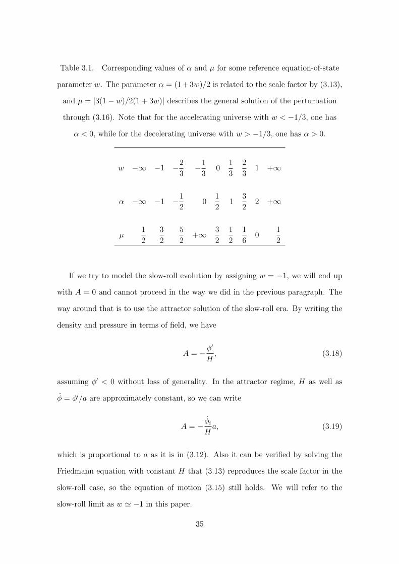
Table 3.1. Corresponding values of α and µ for some reference equation-of-state

parameter w. The parameter α = (1 + 3w)/2 is related to the scale factor by (3.13),

and µ = |3(1− w)/2(1 + 3w)| describes the general solution of the perturbation

through (3.16). Note that for the accelerating universe with w < −1/3, one has

α < 0, while for the decelerating universe with w > −1/3, one has α > 0.

w −∞ −1 −2

3−1

30

1

3

2

31 +∞

α −∞ −1 −1

20

1

21

3

22 +∞

µ1

2

3

2

5

2+∞ 3

2

1

2

1

60

1

2

If we try to model the slow-roll evolution by assigning w = −1, we will end up

with A = 0 and cannot proceed in the way we did in the previous paragraph. The

way around that is to use the attractor solution of the slow-roll era. By writing the

density and pressure in terms of field, we have

A = −φ′

H, (3.18)

assuming φ′ < 0 without loss of generality. In the attractor regime, H as well as

φ = φ′/a are approximately constant, so we can write

A = − φiHa, (3.19)

which is proportional to a as it is in (3.12). Also it can be verified by solving the

Friedmann equation with constant H that (3.13) reproduces the scale factor in the

slow-roll case, so the equation of motion (3.15) still holds. We will refer to the

slow-roll limit as w ' −1 in this paper.

35

For the superinflationary universe with w < −1, we model it by the Lagrangian,

P = −X − V (φ), (3.20)

with the sign of the kinetic term reversed. With the requirement ρ = −X + V > 0,

one generally has V > X > 0, and the scale factor still evolves as (3.13). By

substituting the original definition of A with

A =a√−ρ− PH

, (3.21)

it turns out that the equation of motion of the curvature perturbation can still be

written in the form of the Mukhanov-Sasaki equation (3.8), and the rest of the

analysis follows.

3.2 Assumption and Character of the Small-Scale

Solution

The common assumption on the initial condition is that the mode solution ap-

proaches the Minkowski limit in the short-wavelength limit,

u(η) =1

(2π)3/2√

2ke−ikη (for kη →∞). (3.22)

The Whittaker function that matches this form when z 1 is

W0,µ(2iz) = e−iz[1 +O

(1

z

)]. (3.23)

Therefore, the requirement of matching the adiabatic vacuum picks out the solution,

u(ξ) =eiκ/α

(2π)3/2√

2aiHiκW0,µ

[2iκ

(ξ +

1

α

)]. (3.24)

If at early times of the inflationary history, the universe is initially accelerat-

ing and evolves with a constant equation of state, then by assuming the adiabatic

vacuum at the sub-horizon limit, we obtain the initial condition (3.24). This sub-

horizon initial condition, combined with the quasi-de Sitter expansion, predicts the

36

observed nearly scale invariant super-horizon spectrum in the ΛCDM universe. One

of the reasons that make this scenario attractive is that the quantum fluctuations

we learn well in the local Minkowski spacetime, after being stretched to the cosmic

scale by inflation, also form the seed of the cosmic structure.

When applying the limit (3.22) to a decelerating universe, this sub-horizon as-

sumption becomes acausal. In the decelerating universe, the Hubble horizon grows

faster than the perturbations do, just like in the late-time universe dominated by

matter or radiation. The sub-horizon spectrum is therefore formed after the super-

horizon modes enter the horizon. The estimation we make to the super-horizon

spectrum is then based on that, after the modes enter the horizon, they must fall in

the vacuum state at the small-scale limit. Through the analysis in the next section,

we will see that the large-scale power suppression caused by the preinflation kinetic

era actually originates from the super-horizon spectrum deduced from this picture.

3.3 Scaling Relation

The power spectrum of R is defined through the expectation value of R2(x, t),

〈R2(x, t)〉 =

∫dk

kP (k). (3.25)

Expanding R in terms of the creation and annihilation operators,

R(x, t) =

∫d3k

[akRk(t)e

ik·x + a†kR∗k(t)e

−ik·x], (3.26)

and using the commutator

[ak, a†k′ ] = δ3(k− k′), (3.27)

one finds that

P (k) = 4πk3|Rk|2. (3.28)

37

Recalling that R = −u/A, we find that, for w 6= −1 (so α 6= −1), the power

spectrum given by the solution (3.24) is

P =H2i κ

2|1 + αξ|−2/α

π|1 + α|

∣∣∣∣W0,µ

[2iκ

(ξ +

1

α

)]∣∣∣∣2 . (3.29)

For the slow-roll case, we approximate A by the slow-roll limit (3.19), and the mode

function in that limit is then given by (3.24) with w ' −1. In terms of the slow-roll

parameter,

ε ≡ 1

16π

(1

V

∂V

∂φ

)2

=4πφ2

H2, (3.30)

the power spectrum at the slow-roll limit is given by

P =H2i κ

2|1 + αξ|−2/α

πε

∣∣∣∣W0, 32

[2iκ

(ξ +

1

α

)]∣∣∣∣2 . (3.31)

Using the small-argument expansion of the Whittaker function [96], the super-

horizon limits of the power spectrum are found for different ranges of w. For w <

−1/3 and w > 1 except w = −1, one has

Pκ1 =H2i Γ2(2µ)

πΓ2(µ+ 12)|1 + α|

∣∣∣α2

∣∣∣2µ−1

κ−2µ+3. (3.32)

For w ' −1, the slow-roll power spectrum (3.31) recovers the familiar scale-invariant

spectrum

Pκ1 =H2i

πε. (3.33)

For −1/3 < w < 1, the super-horizon power spectrum decays with time, given by

Pκ1 =H2i Γ2(2µ)

πΓ2(µ+ 12)|1 + α|

∣∣∣α2

∣∣∣2µ−1

κ−2µ+3T (ξ), (3.34)

with the time-dependence

T (ξ) = |1 + αξ|−6(1−w)/(1+3w). (3.35)

For w = 1, the spectrum is

Pκ1 =H2i

3π2κ3T (ξ), (3.36)

38

with

T (ξ) =

∣∣∣∣ln [2iκ(ξ +1

α

)]+ γ − 2 ln 2

∣∣∣∣2 , (3.37)

where γ is the Euler-Mascheroni constant.

We can summarize the power-law relations of the super-horizon power spectrum

with respect to the normalized wavenumber κ by the scaling relation5

P ∝ κ−2µ+3, (3.38)

where the correspondence between the case of w ' −1 and the slow-roll limit is

understood. For the convenience of readers, we also state this result in terms of the

more familiar parameter, w. For w < −1/3 and w > 1,

P ∝ κ6(1+w)/(1+3w). (3.39)

For −1/3 < w < 1,

P ∝ κ12w/(1+3w). (3.40)

The super-horizon behavior of the spectrum can be divided into three types

according to the scaling relation. Some typical cases are plotted in Figure 3.1. For

µ = 3/2, the spectrum is scale-invariant. This is the case for w ' −1 (slow-roll)

and w = 0. When µ < 3/2, the spectrum is blue-tilted and the power is lower

than the scale-invariant spectrum at super-horizon scales. This is attainable from

the positive-pressure (w > 0) or superinflation era (w < −1). In the third case, the

super-horizon spectrum is red-tilted, which is achieved when µ > 3/2, or equivalently

an era with −1 < w < 0 except w = −1/3 (Figure 3.2). Here we reiterate that the

spectra obtained are based on the adiabatic vacuum (3.22), where the corresponding

initial condition for the decelerating universe (w > −1/3) is acausal.

5This relation is also derived in [97] as the approximation to the super-horizon spectrum at

the end of the multi-stage inflationary evolution. The authors focus on the recursive matrix

formalism of the multi-stage preinflationary era, with the assumption that every preinflation era

is an accelerating expansion (or decelerating contraction in the bounce inflation scenario).

39

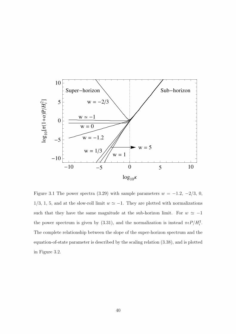
Sub-horizonSuper-horizon

w = -1.2

w > -1

w = -23

w = 0

w = 13w = 1

w = 5

-10 -5 0 5 10

-10

-5

0

5

10

log10Κ

log

10@ΠH1+ΑLPH

i2D

Figure 3.1 The power spectra (3.29) with sample parameters w = −1.2, −2/3, 0,

1/3, 1, 5, and at the slow-roll limit w ' −1. They are plotted with normalizations

such that they have the same magnitude at the sub-horizon limit. For w ' −1

the power spectrum is given by (3.31), and the normalization is instead πεP/H2i .

The complete relationship between the slope of the super-horizon spectrum and the

equation-of-state parameter is described by the scaling relation (3.38), and is plotted

in Figure 3.2.

40

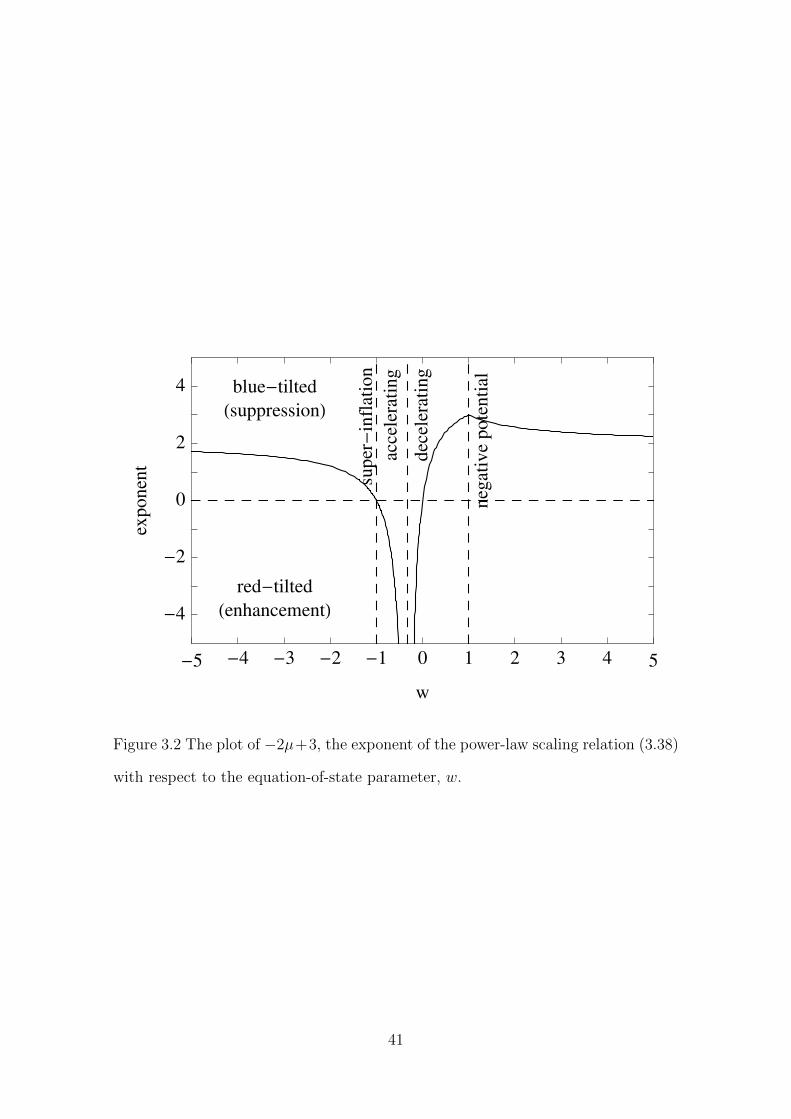
blue-tilted

HsuppressionL

red-tilted

HenhancementL

sup

er-

infl

atio

n

acce

lera

tin

g

dec

eler

atin

g

neg

ativ

ep

ote

nti

al

-5 -4 -3 -2 -1 0 1 2 3 4 5

-4

-2

0

2

4

w

exp

on

ent

Figure 3.2 The plot of −2µ+3, the exponent of the power-law scaling relation (3.38)

with respect to the equation-of-state parameter, w.

41

42

Chapter 4

Evolution of the Power Spectrum

As the universe evolves from the preinflationary era to the inflationary era, the

equation of state changes accordingly. To understand how the initial spectrum of

the preinflationary era is constantly shaped by the expansion of the background

geometry, eventually evolving into the super-horizon spectrum, we develop a use-

ful technique to analyze this process: the spectrum evolution. By analyzing the

evolution of the spectrum, we find that the character of the long-wavelength spec-

trum at the end of inflation actually reflects the nature of the initial state in the

preinflationary era. If at early times before the onset of inflation, the universe is

initially described by some adiabatic vacuum in the background with constant equa-

tion of state, the power spectrum is given by (3.29) during that era. As the universe

evolves with time, although the power spectrum transforms continuously, the spec-

tral shape at the long-wavelength limit is nevertheless not affected by the evolution;

it is preserved in the late-time spectrum.

We demonstrate in this chapter that the spectra can be radically different at

large scales for distinct initial vacua. Particularly, if the universe transits from a

kinetic era into the inflation era, the large-scale spectrum is suppressed because of

the initial adiabatic vacuum assumed in the kinetic era. If the initial vacuum is

different—for example, changed by an earlier accelerating era before the kinetic era,

43

as discussed in this section—the large-scale spectrum may even become enhanced.

We compare the evolution of the power spectrum in three cases, modeled phe-

nomenologically by the single field dynamics. The first one is a single slow-roll era

(denoted as era C) with Hubble parameter HC . The second one is the slow-roll

era (era C) preceded by a kinetic era (era B). In the third case we add one more

slow-roll era (era A), with Hubble parameter HA, before the kinetic era (era B),

which is again followed by the slow-roll era (era C). When applicable, the quantities

at the transition from era A to B are denoted by subscript 1 (so, for example, the

scale factor at the transition is equal to a1), and those at the transition from B to

C are by subscript 2.

In view of the acausal character of the adiabatic vacuum in the initially deceler-

ating era (the second case with only era B and C), we also analyze the case of having

a superinflation era (era S) before the slow-roll era (era C), which also implies power

suppression at large scales but is free from the acausal property. Analogously, the

quantities at the transition from era S to C are denoted by subscript 2.

4.1 Slow-Roll

In the slow-roll era (era C), the general solution to the mode function at the slow-roll

limit w ' −1 is

uC = C+

(1− i aC

kC

)e−ikC/aC

+ C−

(1 + i

aC

kC

)eikC/aC , (4.1)

where kC = k/a2H2 and aC = a/a2 = [1− a2H2(η − η2)]−1. Here a2 and H2 can be

viewed as quantities at some reference time, η2. The notations are chosen for the

convenience of later comparison and should not cause confusion. Note that in the

slow-roll era, one can approximate HC ≈ H2 as a constant. The normalized power

44

spectrum is given by

PC =k3C

a2C

∣∣∣∣C+

(1− i aC

kC

)e−ikC/aC

+C−

(1 + i

aC

kC

)eikC/aC

∣∣∣∣2 , (4.2)

where C± =√a2H2C±, and

PC =εP

16π2H2C

, (4.3)

ε =4πφ2

H2

∣∣∣∣∣C

. (4.4)

are the normalized power spectrum and the slow-roll parameter evaluated in era C,

respectively.

In the adiabatic vacuum (3.22), only the second term in (4.1) remains, and the

mode function reduces to

uC =1

(2π)3/2√

2k

(1 + i

aC

kC

)eikC/aC . (4.5)

The power spectrum is

PC =1

16π3

(1 +

k2C

a2C

), (4.6)

which recovers the well-known form in the super-horizon limit,

P =1

π

(H2C

ε

). ( kC 1 at aC = 1 ) (4.7)

The comoving horizon size decreases with time, moving toward the right to the small

scales in Figure 4.1. After the mode exits the horizon, lying on the left-hand side of

the horizon scale, the power stays scale-invariant.

4.2 Kinetic—Slow-Roll

In the second case, the energy density is dominated by the kinetic energy at η < η2,

with

H ≈ −√

4π

3

φ′

a, (4.8)

45

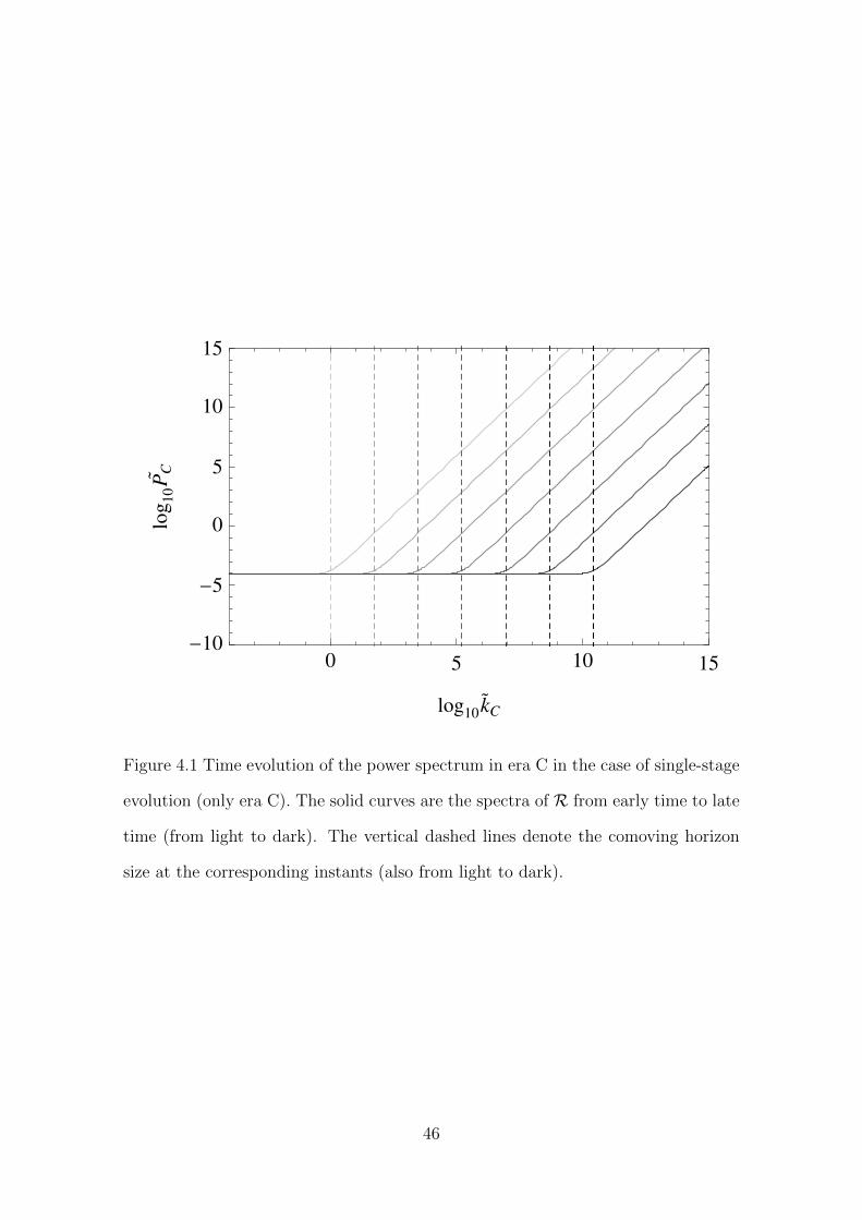
0 5 10 15-10

-5

0

5

10

15

log10k

C

log

10P

C

Figure 4.1 Time evolution of the power spectrum in era C in the case of single-stage

evolution (only era C). The solid curves are the spectra of R from early time to late

time (from light to dark). The vertical dashed lines denote the comoving horizon

size at the corresponding instants (also from light to dark).

46

assuming φ′ ≤ 0 without lose of generality. In the kinetic era, w = 1 and the mode

function can be written in terms of the Hankel functions,

uB =B+aBH(1)0

(1

2kBa

2B

)+B−aBH

(2)0

(1

2kBa

2B

), (4.9)

where we denote kB = k/a1H1 and aB = a/a1 =√

1 + 2a1H1(η − η1). Similarly,

for later convenience, we choose η1 < η2 to be some reference time for era B. The

power spectrum in the kinetic era is given by

PB = k3B

∣∣∣∣B+H(1)0

(1

2kBa

2B

)+B−H

(2)0

(1

2kBa

2B

)∣∣∣∣2 , (4.10)

where B± =√a1H1B±, and

PB =3P

16π2H21

. (4.11)

At η > η2, the universe shifts into the slow-roll stage, and the solution is given

by (4.1). To match the boundary between the eras, we fix the coefficients C+ and

C− by the continuity of R and R′. One finds

C+ =eikC

2kC

[kCH

(1)0,C − (1− ikC)H

(1)1,C

]B+

+[kCH

(2)0,C − (1− ikC)H

(2)1,C

]B−

, (4.12)

C− =e−ikC

2kC

[kCH

(1)0,C − (1 + ikC)H

(1)1,C

]B+

+[kCH

(2)0,C − (1 + ikC)H

(2)1,C

]B−

, (4.13)

where H(1)0,C is the shorthand of H

(1)0 (kC/2) and so on. The power spectrum in era

C is given by (4.2) with C+ and C− substituted by (4.12) and (4.13), respectively.

If the universe is in the adiabatic vacuum in era B, only the second term in (4.9)

presents in the mode function,

uB =1

8πaBH

(2)0

(1

2kBa

2B

), (4.14)

47

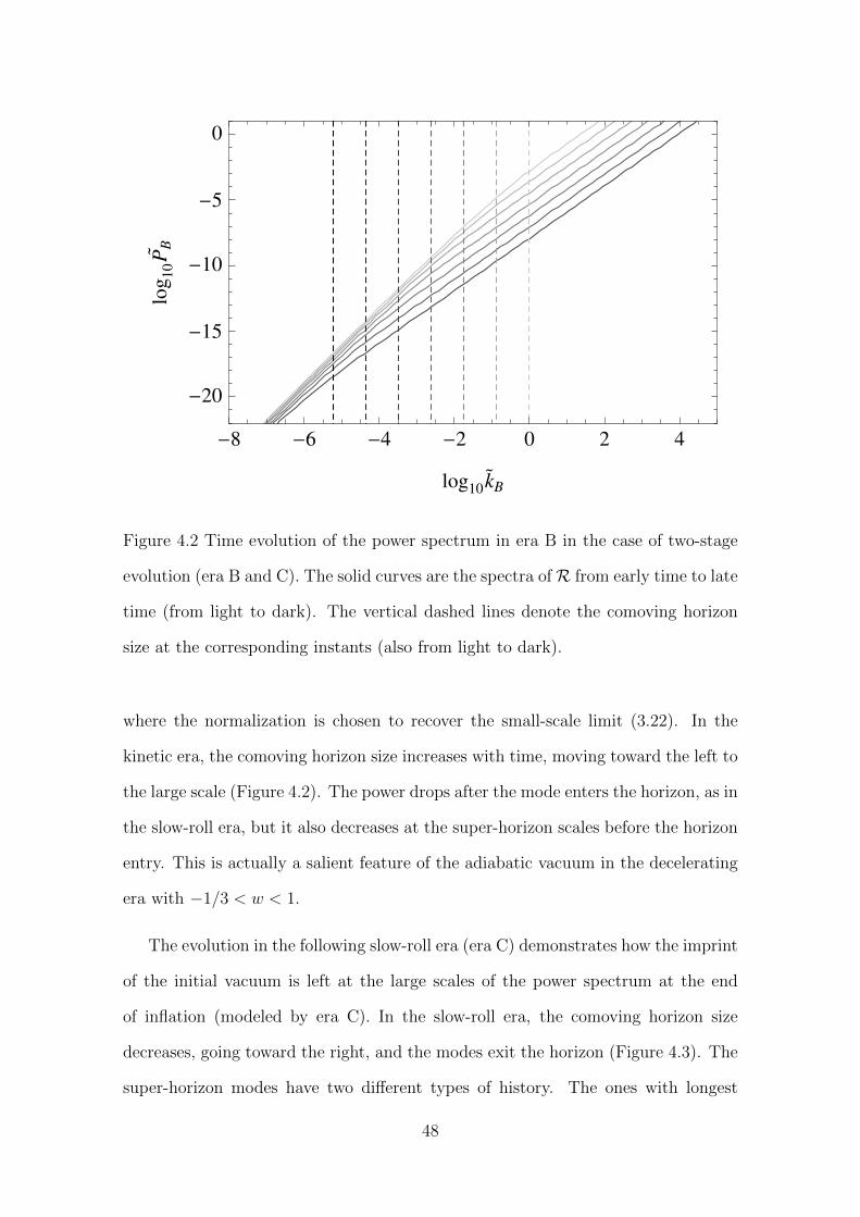
-8 -6 -4 -2 0 2 4

-20

-15

-10

-5

0

log10k

B

log

10P

B

Figure 4.2 Time evolution of the power spectrum in era B in the case of two-stage

evolution (era B and C). The solid curves are the spectra ofR from early time to late



where the normalization is chosen to recover the small-scale limit (3.22). In the

kinetic era, the comoving horizon size increases with time, moving toward the left to

the large scale (Figure 4.2). The power drops after the mode enters the horizon, as in

the slow-roll era, but it also decreases at the super-horizon scales before the horizon

entry. This is actually a salient feature of the adiabatic vacuum in the decelerating

era with −1/3 < w < 1.

The evolution in the following slow-roll era (era C) demonstrates how the imprint

of the initial vacuum is left at the large scales of the power spectrum at the end

of inflation (modeled by era C). In the slow-roll era, the comoving horizon size

decreases, going toward the right, and the modes exit the horizon (Figure 4.3). The

super-horizon modes have two different types of history. The ones with longest

48

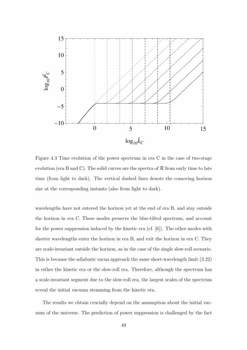
0 5 10 15-10

-5

0

5

10

15

log10k

C

log

10P

C

Figure 4.3 Time evolution of the power spectrum in era C in the case of two-stage

evolution (era B and C). The solid curves are the spectra ofR from early time to late



wavelengths have not entered the horizon yet at the end of era B, and stay outside

the horizon in era C. These modes preserve the blue-tilted spectrum, and account

for the power suppression induced by the kinetic era (cf. [6]). The other modes with

shorter wavelengths enter the horizon in era B, and exit the horizon in era C. They

are scale-invariant outside the horizon, as in the case of the single slow-roll scenario.

This is because the adiabatic vacua approach the same short-wavelength limit (3.22)

in either the kinetic era or the slow-roll era. Therefore, although the spectrum has

a scale-invariant segment due to the slow-roll era, the largest scales of the spectrum

reveal the initial vacuum stemming from the kinetic era.

The results we obtain crucially depend on the assumption about the initial vac-

uum of the universe. The prediction of power suppression is challenged by the fact

49

that it originates from the blue-tilted super-horizon initial spectrum in the prein-

flation decelerating era, in which the super-horizon modes have not been in causal

contact throughout the history. We demonstrate this point by an illustration show-

ing the evolution of the Fourier wavelengths and the Hubble horizon (Figure 4.4).

In the decelerating universe, such as the initial kinetic era, the Hubble horizon

grows faster than the Fourier wavelengths do. At the end of the initial decelerat-

ing era and the beginning of the accelerating inflation, the modes that are about

to enter the horizon—those who are the origin of the suppressed large-scale modes

today—will soon be expanded and kept outside the horizon by inflation. If the uni-

verse starts with the decelerating era before inflation, these mode are then insulated

from any sub-horizon dynamics throughout the history. Therefore, the spectrum

of the perturbations beyond the horizon size at the end of the decelerating era is

not the consequence of causal physics, and the common approach of deducing the

initial conditions through requiring the spectrum recover the Minkowski limit at

the sub-horizon scale is therefore a posteriori. This is of the same footing as the

“horizon problem” the big bang cosmology faced before the picture of inflation was

introduced.

4.3 Slow-Roll—Kinetic—Slow-Roll

With the additional slow-roll era (era A) prepending the kinetic era (era B), we

simply apply solution (4.1) at η < η1,

uA = A+

(1− i aA

kA

)e−ikA/aA

+ A−

(1 + i

aA

kA

)eikA/aA , (4.15)

50

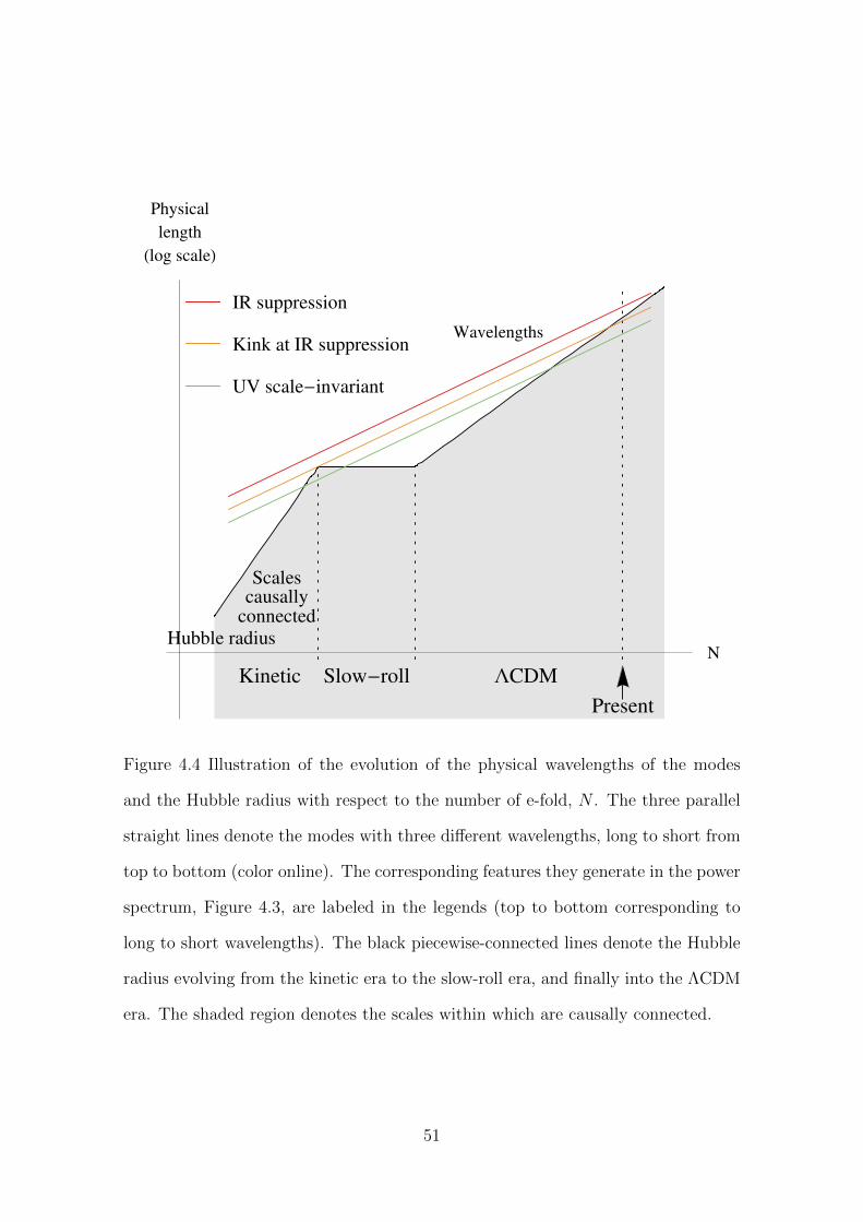
Kinetic Slow-roll LCDM

Present

Hubble radius

Wavelengths

Scalescausally

connected

IR suppression

Kink at IR suppression

UV scale-invariant

N

Physical

length

Hlog scaleL

Figure 4.4 Illustration of the evolution of the physical wavelengths of the modes

and the Hubble radius with respect to the number of e-fold, N . The three parallel

straight lines denote the modes with three different wavelengths, long to short from

top to bottom (color online). The corresponding features they generate in the power

spectrum, Figure 4.3, are labeled in the legends (top to bottom corresponding to

long to short wavelengths). The black piecewise-connected lines denote the Hubble

radius evolving from the kinetic era to the slow-roll era, and finally into the ΛCDM

era. The shaded region denotes the scales within which are causally connected.

51

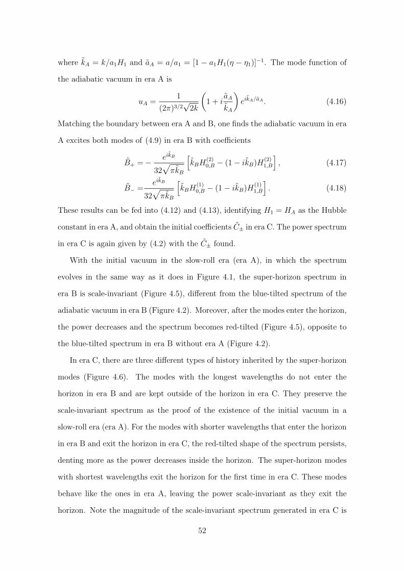
where kA = k/a1H1 and aA = a/a1 = [1 − a1H1(η − η1)]−1. The mode function of

the adiabatic vacuum in era A is

uA =1

(2π)3/2√

2k

(1 + i

aA

kA

)eikA/aA . (4.16)

Matching the boundary between era A and B, one finds the adiabatic vacuum in era

A excites both modes of (4.9) in era B with coefficients

B+ =− eikB

32√πkB

[kBH

(2)0,B − (1− ikB)H

(2)1,B

], (4.17)

B− =eikB

32√πkB

[kBH

(1)0,B − (1− ikB)H

(1)1,B

]. (4.18)

These results can be fed into (4.12) and (4.13), identifying H1 = HA as the Hubble

constant in era A, and obtain the initial coefficients C± in era C. The power spectrum

in era C is again given by (4.2) with the C± found.

With the initial vacuum in the slow-roll era (era A), in which the spectrum

evolves in the same way as it does in Figure 4.1, the super-horizon spectrum in

era B is scale-invariant (Figure 4.5), different from the blue-tilted spectrum of the

adiabatic vacuum in era B (Figure 4.2). Moreover, after the modes enter the horizon,

the power decreases and the spectrum becomes red-tilted (Figure 4.5), opposite to

the blue-tilted spectrum in era B without era A (Figure 4.2).

In era C, there are three different types of history inherited by the super-horizon

modes (Figure 4.6). The modes with the longest wavelengths do not enter the

horizon in era B and are kept outside of the horizon in era C. They preserve the

scale-invariant spectrum as the proof of the existence of the initial vacuum in a

slow-roll era (era A). For the modes with shorter wavelengths that enter the horizon

in era B and exit the horizon in era C, the red-tilted shape of the spectrum persists,

denting more as the power decreases inside the horizon. The super-horizon modes

with shortest wavelengths exit the horizon for the first time in era C. These modes

behave like the ones in era A, leaving the power scale-invariant as they exit the

horizon. Note the magnitude of the scale-invariant spectrum generated in era C is

52

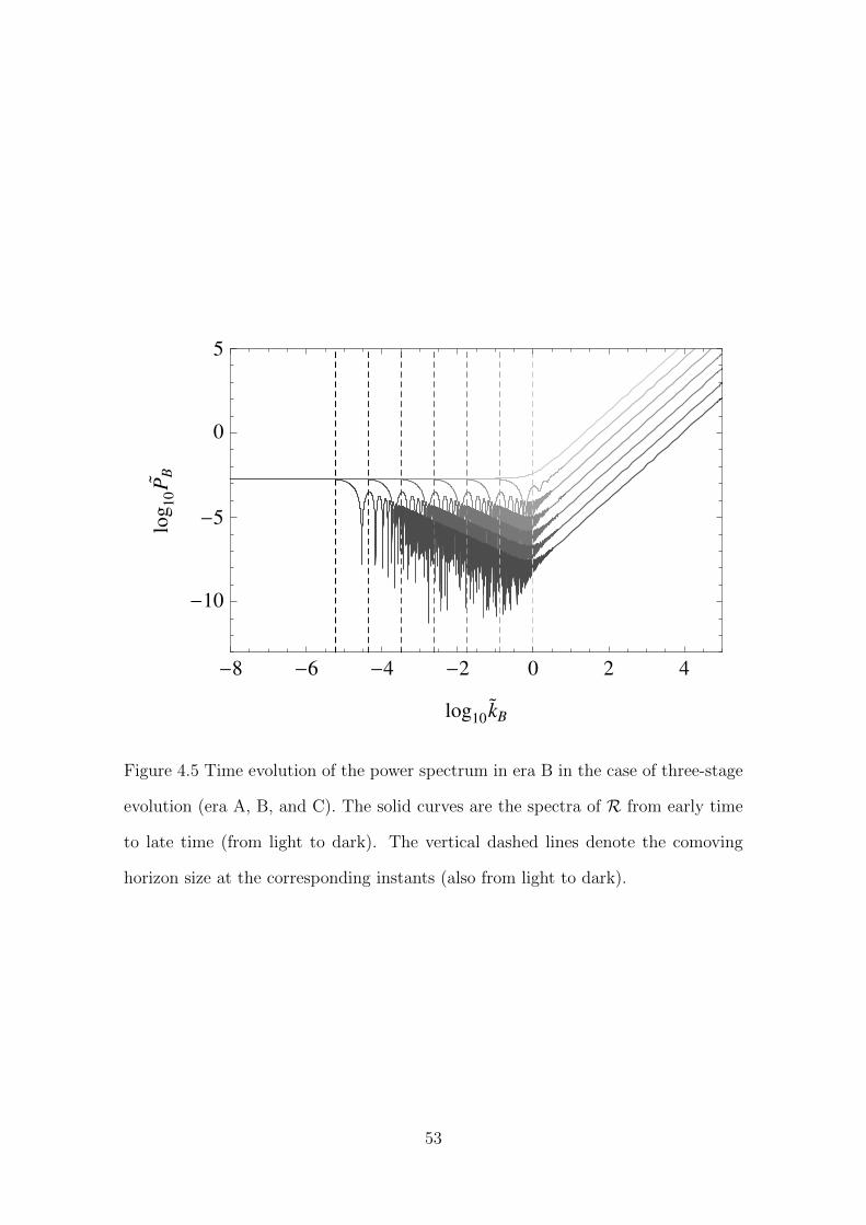
-8 -6 -4 -2 0 2 4

-10

-5

0

5

log10k

B

log

10P

B

Figure 4.5 Time evolution of the power spectrum in era B in the case of three-stage

evolution (era A, B, and C). The solid curves are the spectra of R from early time

to late time (from light to dark). The vertical dashed lines denote the comoving

horizon size at the corresponding instants (also from light to dark).

53

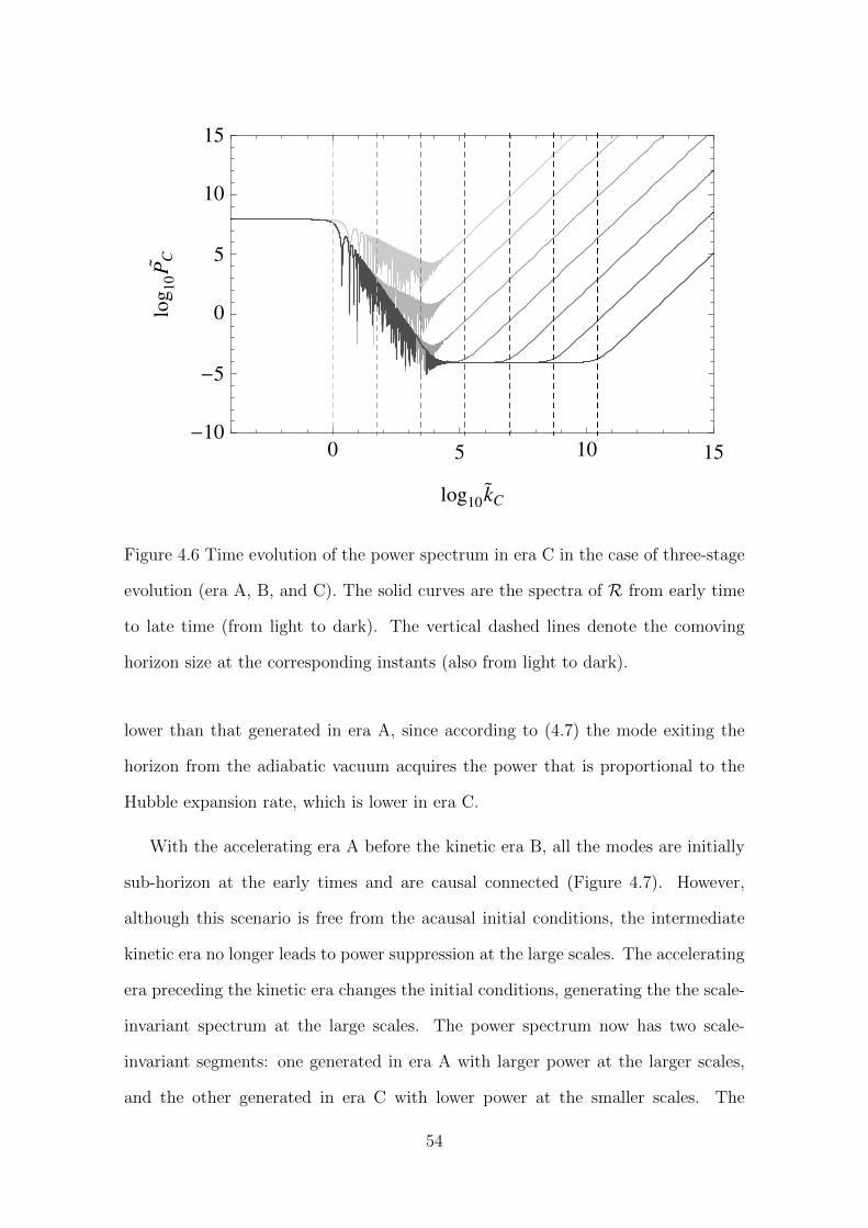
0 5 10 15-10

-5

0

5

10

15

log10k

C

log

10P

C

Figure 4.6 Time evolution of the power spectrum in era C in the case of three-stage

evolution (era A, B, and C). The solid curves are the spectra of R from early time

to late time (from light to dark). The vertical dashed lines denote the comoving

horizon size at the corresponding instants (also from light to dark).

lower than that generated in era A, since according to (4.7) the mode exiting the

horizon from the adiabatic vacuum acquires the power that is proportional to the

Hubble expansion rate, which is lower in era C.

With the accelerating era A before the kinetic era B, all the modes are initially

sub-horizon at the early times and are causal connected (Figure 4.7). However,

although this scenario is free from the acausal initial conditions, the intermediate

kinetic era no longer leads to power suppression at the large scales. The accelerating

era preceding the kinetic era changes the initial conditions, generating the the scale-

invariant spectrum at the large scales. The power spectrum now has two scale-

invariant segments: one generated in era A with larger power at the larger scales,

and the other generated in era C with lower power at the smaller scales. The

54

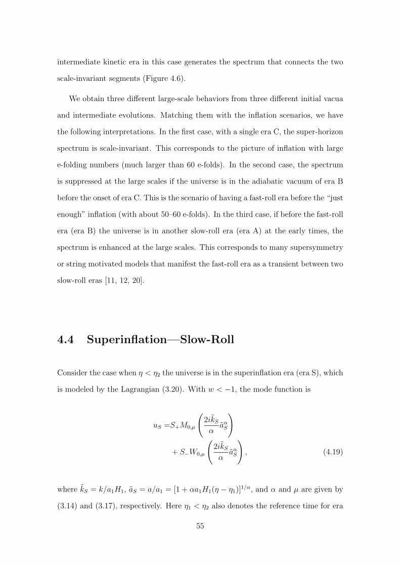
intermediate kinetic era in this case generates the spectrum that connects the two

scale-invariant segments (Figure 4.6).

We obtain three different large-scale behaviors from three different initial vacua

and intermediate evolutions. Matching them with the inflation scenarios, we have

the following interpretations. In the first case, with a single era C, the super-horizon

spectrum is scale-invariant. This corresponds to the picture of inflation with large

e-folding numbers (much larger than 60 e-folds). In the second case, the spectrum

is suppressed at the large scales if the universe is in the adiabatic vacuum of era B

before the onset of era C. This is the scenario of having a fast-roll era before the “just

enough” inflation (with about 50–60 e-folds). In the third case, if before the fast-roll

era (era B) the universe is in another slow-roll era (era A) at the early times, the

spectrum is enhanced at the large scales. This corresponds to many supersymmetry

or string motivated models that manifest the fast-roll era as a transient between two

slow-roll eras [11, 12, 20].

4.4 Superinflation—Slow-Roll

Consider the case when η < η2 the universe is in the superinflation era (era S), which

is modeled by the Lagrangian (3.20). With w < −1, the mode function is

uS =S+M0,µ

(2ikSα

aαS

)

+ S−W0,µ

(2ikSα

aαS

), (4.19)

where kS = k/a1H1, aS = a/a1 = [1 + αa1H1(η − η1)]1/α, and α and µ are given by

(3.14) and (3.17), respectively. Here η1 < η2 also denotes the reference time for era

55

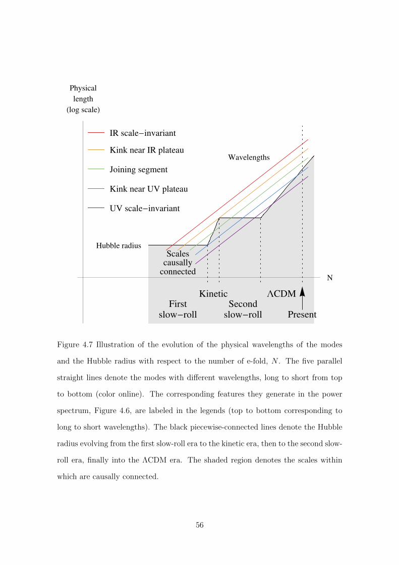
Firstslow-roll

KineticSecond

slow-roll

LCDM

Present

Hubble radius

Wavelengths

Scalescausally

connected

IR scale-invariant

Kink near IR plateau

Joining segment

Kink near UV plateau

UV scale-invariant

N

Physical

length

Hlog scaleL

Figure 4.7 Illustration of the evolution of the physical wavelengths of the modes

and the Hubble radius with respect to the number of e-fold, N . The five parallel

straight lines denote the modes with different wavelengths, long to short from top

to bottom (color online). The corresponding features they generate in the power

spectrum, Figure 4.6, are labeled in the legends (top to bottom corresponding to

long to short wavelengths). The black piecewise-connected lines denote the Hubble

radius evolving from the first slow-roll era to the kinetic era, then to the second slow-

roll era, finally into the ΛCDM era. The shaded region denotes the scales within

which are causally connected.

56

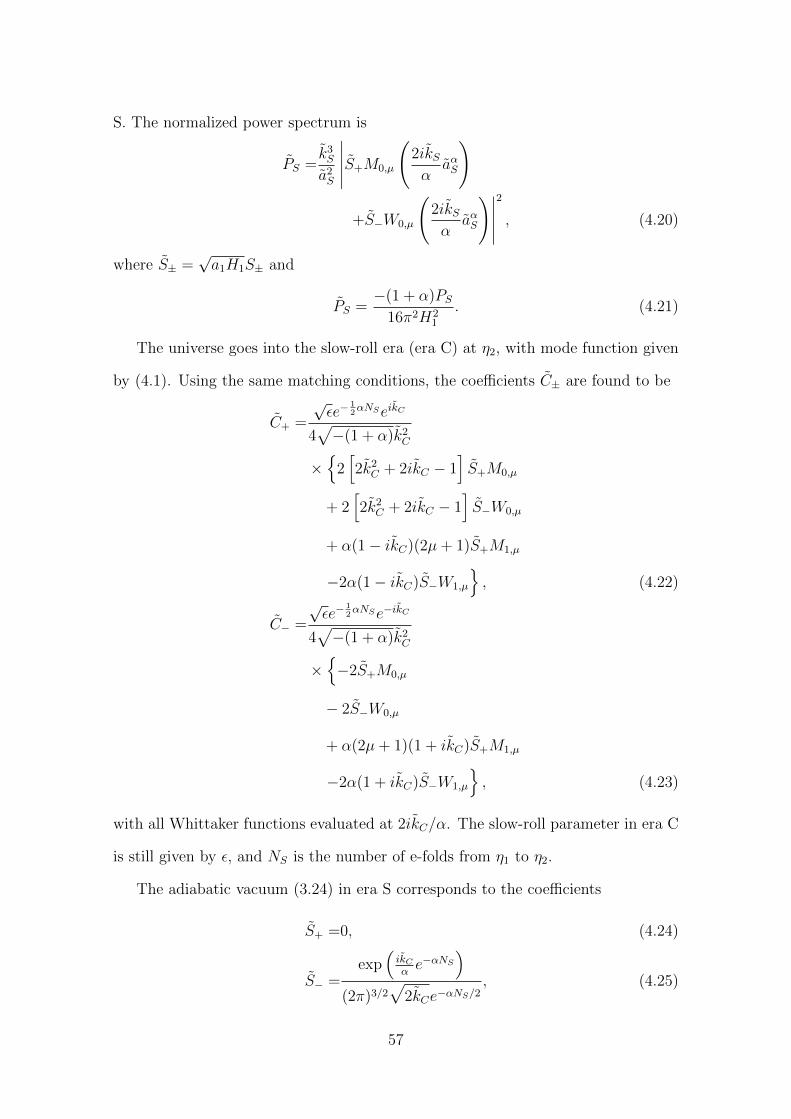
S. The normalized power spectrum is

PS =k3S

a2S

∣∣∣∣∣S+M0,µ

(2ikSα

aαS

)

+S−W0,µ

(2ikSα

aαS

)∣∣∣∣∣2

, (4.20)

where S± =√a1H1S± and

PS =−(1 + α)PS

16π2H21

. (4.21)

The universe goes into the slow-roll era (era C) at η2, with mode function given

by (4.1). Using the same matching conditions, the coefficients C± are found to be

C+ =

√εe−

12αNSeikC

4√−(1 + α)k2

C

×

2[2k2

C + 2ikC − 1]S+M0,µ

+ 2[2k2

C + 2ikC − 1]S−W0,µ

+ α(1− ikC)(2µ+ 1)S+M1,µ

−2α(1− ikC)S−W1,µ

, (4.22)

C− =

√εe−

12αNSe−ikC

4√−(1 + α)k2

C

×−2S+M0,µ

− 2S−W0,µ

+ α(2µ+ 1)(1 + ikC)S+M1,µ

−2α(1 + ikC)S−W1,µ

, (4.23)

with all Whittaker functions evaluated at 2ikC/α. The slow-roll parameter in era C

is still given by ε, and NS is the number of e-folds from η1 to η2.

The adiabatic vacuum (3.24) in era S corresponds to the coefficients

S+ =0, (4.24)

S− =exp

(ikCαe−αNS

)(2π)3/2

√2kCe−αNS/2

, (4.25)

57

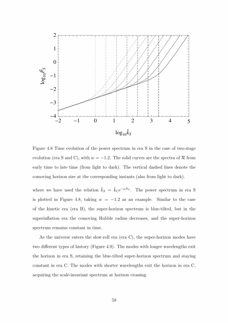
-2 -1 0 1 2 3 4 5-4

-3

-2

-1

0

1

2

log10k

S

log

10P

S

Figure 4.8 Time evolution of the power spectrum in era S in the case of two-stage

evolution (era S and C), with w = −1.2. The solid curves are the spectra of R from

early time to late time (from light to dark). The vertical dashed lines denote the

comoving horizon size at the corresponding instants (also from light to dark).

where we have used the relation kS = kCe−αNS . The power spectrum in era S

is plotted in Figure 4.8, taking w = −1.2 as an example. Similar to the case

of the kinetic era (era B), the super-horizon spectrum is blue-tilted, but in the

superinflation era the comoving Hubble radius decreases, and the super-horizon

spectrum remains constant in time.

As the universe enters the slow-roll era (era C), the super-horizon modes have

two different types of history (Figure 4.9). The modes with longer wavelengths exit

the horizon in era S, retaining the blue-tilted super-horizon spectrum and staying

constant in era C. The modes with shorter wavelengths exit the horizon in era C,

acquiring the scale-invariant spectrum at horizon crossing.

58

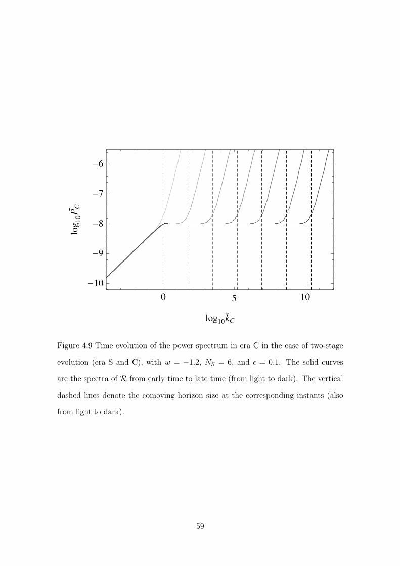
0 5 10

-10

-9

-8

-7

-6

log10k

C

log

10P

C

Figure 4.9 Time evolution of the power spectrum in era C in the case of two-stage

evolution (era S and C), with w = −1.2, NS = 6, and ε = 0.1. The solid curves

are the spectra of R from early time to late time (from light to dark). The vertical

dashed lines denote the comoving horizon size at the corresponding instants (also

from light to dark).

59

60

Chapter 5

Two-field cascade inflation

After establishing the understanding of the spectrum evolution in multi-stage infla-

tion using the ad hoc single-field analysis, in this chapter we calculate the spectrum

generated by a two-stage inflation model from the given potential. The purposes

are to show that the evolution pattern we obtain in the single-field analysis is also

reflected in the two-field dynamics, and to check whether the large-scale power is

suppressed due to the coupling between the two fields.

5.1 Background Evolution and the Attractor So-

lution

We investigate a simple two-field cascade inflation, which is driven by a heavy scalar

field ψ and a light scalar field φ with the action

S =

∫d4x√−g[−1

2∂αφ∂

αφ− 1

2∂αψ∂

αψ − V (φ, ψ)

]. (5.1)

In large field inflation, the field operates at the super-Plankian scale when the coeffi-

cient of the kinetic term is normalized to 1/2. If the field value is of the order of the

Planck mass, MP = 1/√G, the energy scale of inflation is determined by the mass of

the field. The typical evolution can therefore be divided into four stages. The first

61

stage is the inflationary era driven by the heavy field, with fields starting far away

from the potential minimum and rolling down alone the hillside of the potential. At

the second stage the heavy field falls into the potential minimum and oscillates with

damping amplitude. As the energy drops to the scale of the light field mass, the

universe enters the third stage in which the light field initiates the other inflation

era. Finally at the fourth stage the light field decays, ending the inflation, and the

standard ΛCDM evolution begins.

Consider the cascade inflation realized by the potential

V (φ, ψ) =λ′

2φ2ψ2 +

1

2m2φ2. (5.2)

The heavy-field inflation is driven by the coupling term λ′φ2ψ2/2, and the light-field

inflation is driven by the mass term m2φ2/2. At the stage of heavy-field inflation,

the fields follow the attractor solutions, which can be obtained through expressing

the equations of motion in terms of the number of e-folds, N ≡ ln(a/ai), where ai

is some initial scale factor. The Friedmann equation is

H2 =8π3V

1− 4π3

[(dφdN

)2+(dψdN

)2] , (5.3)

where H = a/a. The dots denote the derivatives with respect to t. The equations

of motion can be casted into the form

d2φ

dN2− 4π

[(dφ

dN

)2

+

(dψ

dN

)2

− 3

4π

]

×(dφ

dN+

1

8πV

∂V

∂φ

)= 0, (5.4)

d2ψ

dN2− 4π

[(dφ

dN

)2

+

(dψ

dN

)2

− 3

4π

]

×(dψ

dN+

1

8πV

∂V

∂ψ

)= 0. (5.5)

It can be shown that the attractor solutions satisfy

dφ

dN=− 1

8πV

∂V

∂φ, (5.6)

dψ

dN=− 1

8πV

∂V

∂ψ, (5.7)

62

provided (dφ/dN)2 +(dψ/dN)2−3/4π < 0 as constrained by (5.3).1 With potential

dominated by λ′φ2ψ2/2, the attractor solutions are

φ(N) =

√φ2i −

1

2π(N −Ni), (5.8)

ψ(N) =

√ψ2i −

1

2π(N −Ni), (5.9)

where the subscripts i denote the initial values.

At the second stage, ψ exits the slow-roll regime and oscillates at the minimum of

the potential with its amplitude damped with time. The potential is still dominated

by the coupling term before the next inflation begins. During the oscillatory stage,

φ remains slow roll, while ψ acquires a large kinetic energy that is of the same

order of the potential energy, ψ2 ∼ λ′φ2ψ2 ∼ H2, and the energy density evolves

effectively according to w = 0 (zero pressure). Ignoring the kinetic energy of φ in

the Friedmann equation, we have(dψ

dN

)2

+λ′φ2

H2ψ2 =

3

4π. (5.10)

With A ≡ H/√λ′φ, we parametrize ψ and dψ/dN by the amplitude A and the

phase θ,

dψ

dN=

√3

4πcos θ, (5.11)

ψ =

√3

4πA sin θ. (5.12)

Combining (5.5) and (5.10), we obtain a set of differential equations of A and θ

dA

dN=− A cos2 θ

(3 +

1

φ

dφ

dN

), (5.13)

dθ

dN=

1

A+ cos θ sin θ

(3 +

1

φ

dφ

dN

). (5.14)

1For φ, the type of the attractor considered here is the horizontal trajectory on the φ–dφ/dN

plane; that is, the one with (d/dφ)(dφ/dN) = 0. Since d2φ/dN2 = (dφ/dN)× (d/dφ)(dφ/dN), we

obtain the condition for the attractor solution with non-vanishing dφ/dN as d2φ/dN2 = 0, which

in turn leads to (5.6). Similar argument applies to ψ.

63

Among the two terms contributing to the frequency dθ/dN , the first term 1/A is of

the order of 1/ψ, since A = H/√λ′φ ≈

√λ′φψ/

√λ′φ = ψ. The second term is of

order unity as φ slow rolls. After ψ drops below the Planck mass, 1/A dominates

and θ oscillates rapidly, so we can approximate cos2 θ in (5.13) by 1/2. With φ given

by the slow-roll solution (5.8), A and θ can then be integrated to yield

A(N) = Ai

(1− N −Ni

2πφ2i

)−1/4

e−32

(N−Ni), (5.15)

θ(N) = θi +N −Ni

Ai− (N −Ni)

2

16πφ2iAi

. (5.16)

As the field ψ attenuates, gradually the energy density from the coupling term

is taken over by the m2φ2/2 term. The universe enters the third stage, in which the

other inflation driven by the light-field begins. This stage is effectively described by

the single-field inflation, with the same attractor solution (5.8) for φ.

5.2 Perturbations and Initial Conditions

Here we consider the perturbation to the homogeneous background in the conformal

Newtonian gauge. The field perturbations are

φ(x, t) = φ(t) + δφ(x, t), (5.17)

ψ(x, t) = ψ(t) + δψ(x, t), (5.18)

where φ(t) and ψ(t) denote the background solutions. The equations of motion of

the perturbations in the Fourier space are

δφ+ 3Hδφ+

(k2

a2+∂2V

∂φ2

)δφ =

− ∂2V

∂φ∂ψδψ − 2

∂V

∂φΨ + 4 ˙φΨ, (5.19)

δψ + 3Hδψ +

(k2

a2+∂2V

∂ψ2

)δψ =

− ∂2V

∂φ∂ψδφ− 2

∂V

∂ψΨ + 4 ˙ψΨ, (5.20)

Ψ +HΨ = 4π( ˙φδφ+ ˙ψδψ). (5.21)

64

Note that the energy-momentum tensor of action (5.1) has no velocity perturbations

either anisotropic inertia, so the Einstein equation gives Φ = Ψ. The curvature

perturbation in two-field system is

R = −Ψ−H˙φδφ+ ˙ψδψ

˙φ2 + ˙ψ2. (5.22)

The initial conditions for the sub-horizon modes are set in the era of the heavy-

field inflation by the method of iteration. We first neglect the metric perturbations

Ψ and find the solutions to δφ and δψ at the short-wavelength limit. The initial

conditions for the sub-horizon field perturbations are set as the normalized positive-

frequency solutions. We then feed the initial δφ and δψ back into the Einstein

equations and obtain the initial conditions of Ψ. At the end we perform the consis-

tency check to see whether the initial Ψ obtained are indeed much smaller than δφ

and δψ at the short-wavelength limit.

To solve the field perturbations, first note that the equations of motion (5.19)

and (5.20) can be put into a simpler form by substitute t by the conformal time η,

and introducing the new variables w = aδφ and q = aδψ. Neglecting the metric

perturbation, the equations for w and q are

w′′ +

(k2 +

∂2V

∂φ2− a′′

a

)w =− ∂2V

∂φ∂ψa2q, (5.23)

q′′ +

(k2 +

∂2V

∂ψ2− a′′

a

)q =− ∂2V

∂φ∂ψa2w, (5.24)

where the primes denote the derivatives with respect to the conformal time η. For

k aH the two equations decouple and reduce to the equations of harmonic oscil-

lators

w′′ + k2w = 0, (5.25)

q′′ + k2q = 0. (5.26)

65

After the quantization, the normalized positive-frequency mode functions are

δφ(η) =e−ikη

(2π)3/2√

2k a, (5.27)

δψ(η) =e−ikη

(2π)3/2√

2k a, (5.28)

which are the initial conditions for the sub-horizon field perturbations. Feeding

(5.27) and (5.28) into the Einstein equation

Ψ =1

˙φ2 + ˙ψ2 − k2

4πa2

[˙φδφ+ ˙ψδψ

+

(3H ˙φ+

∂V

∂φ

)δφ+

(3H ˙ψ +

∂V

∂ψ

)δψ

], (5.29)

one obtains the initial conditions for the sub-horizon metric perturbations.

To justify that the metric perturbations are negligible when finding solutions to

the field perturbations, in this paragraph we are going to show that Ψ obtained by

(5.29) is much smaller than δφ and δψ at the short-wavelength limit in the era of

heavy-field inflation. The following discussion in this paragraph assumes k aH.

First note that from (5.8) and (5.9) one has ˙φ ∼ H/φ and ˙ψ ∼ H/ψ. The metric

perturbation (5.29) therefore goes like

Ψ ∼ 1(kaH

)2

[δφ

Hφ+

δψ

Hψ

+

(1

φ+λ′φψ2

H2

)δφ+

(1

ψ+λ′φ2ψ

H2

)δψ

], (5.30)

where we have omitted all the constant coefficients and used the fact that the po-

tential is dominated by λ′φ2ψ2/2 during the heavy-field inflation. From solutions

(5.27) and (5.28) one has

δφ = −Hδφ(

1 +ik

aH

)∼ k

aδφ (5.31)

and similarly for δψ. The first two terms in the bracket of (5.30) then go like

(k/aH) · (δφ/φ) and (k/aH) · (δψ/ψ). Using the Friedmann equation we know that

λ′φψ2/H2 ∼ 1/φ and λ′φ2ψ/H2 ∼ 1/ψ, therefore the last two terms in the bracket

66

of (5.30) go like δφ/φ and δψ/ψ. Since during the heavy-field inflation φ and ψ is

of order O(1) in Planck units, one has

Ψ ∼ 1(kaH

) (δφφ

+δψ

ψ

). (5.32)

Therefore the initial Ψ is indeed much smaller than the initial δφ and δψ at the

limit of k aH in the era of heavy-field inflation.

5.3 Numerical Solution and the CMB Spectrum

The CMB spectrum is found by three steps of numerical calculations. We first obtain

the background dynamics by solving (5.4) and (5.5). The reheating energy scale is

assumed to be 7.19 × 10−4MP ∼ 1016GeV. The evolution of perturbations is then

solved by integrating (5.19), (5.20), and (5.21), with the initial conditions set by

(5.27), (5.28), and (5.29). The spectrum of the curvature perturbations is found by

evolving each Fourier mode until it reaches the steady value after the horizon exit.

The resulting spectrum is then fed into CAMB [43, 44], which is modified to accept

arbitrary initial spectrum represented by an interpolating function, to calculate the

spectrum of the CMB temperature fluctuations.

There are two parameters and four initial conditions in our model. The two

parameters are the coupling constant, λ′, and the mass of the light field, m. The

four initial conditions are the initial values and derivatives of the fields φ and ψ. We

assume that the light field drives about the last 60 e-folds of inflation, so the mass

m is determined by the Hubble scale during inflation deduced by the observation.

The initial derivatives of φ and ψ are set to zero, leaving the system released from

rest and evolving into the attractor solutions.

The initial value of the light field φ determines the behavior of the system in two

ways. First, it determines the energy scale of the heavy-field inflation as well as that

of the oscillatory period, since at the beginning of the oscillatory stage ψ ∼MP and

67

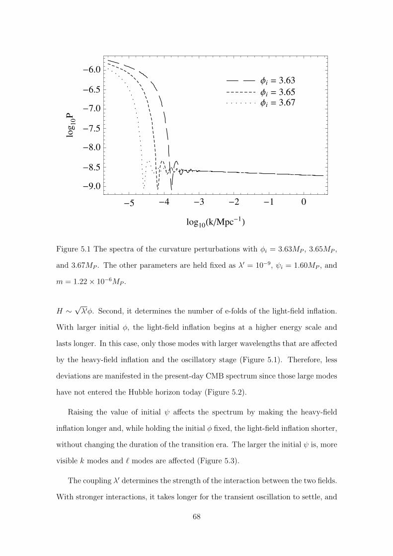
Φi = 3.63

Φi = 3.65Φi = 3.67

-5 -4 -3 -2 -1 0

-9.0

-8.5

-8.0

-7.5

-7.0

-6.5

-6.0

log10HkMpc-1L

log

10P

Figure 5.1 The spectra of the curvature perturbations with φi = 3.63MP , 3.65MP ,

and 3.67MP . The other parameters are held fixed as λ′ = 10−9, ψi = 1.60MP , and

m = 1.22× 10−6MP .

H ∼√λ′φ. Second, it determines the number of e-folds of the light-field inflation.

With larger initial φ, the light-field inflation begins at a higher energy scale and

lasts longer. In this case, only those modes with larger wavelengths that are affected

by the heavy-field inflation and the oscillatory stage (Figure 5.1). Therefore, less

deviations are manifested in the present-day CMB spectrum since those large modes

have not entered the Hubble horizon today (Figure 5.2).

Raising the value of initial ψ affects the spectrum by making the heavy-field

inflation longer and, while holding the initial φ fixed, the light-field inflation shorter,

without changing the duration of the transition era. The larger the initial ψ is, more

visible k modes and ` modes are affected (Figure 5.3).

The coupling λ′ determines the strength of the interaction between the two fields.

With stronger interactions, it takes longer for the transient oscillation to settle, and

68

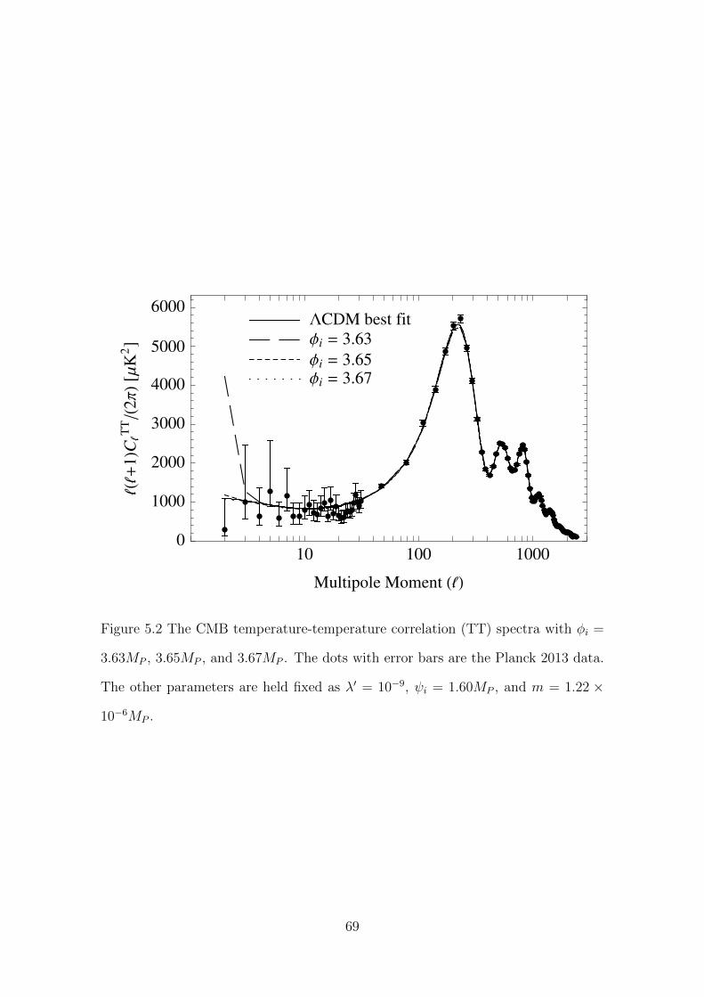
LCDM best fit

Φi = 3.63

Φi = 3.65Φi = 3.67

10 100 10000

1000

2000

3000

4000

5000

6000

Multipole Moment HL

H+

1LC

T

TH

2ΠL@Μ

K2D

Figure 5.2 The CMB temperature-temperature correlation (TT) spectra with φi =

3.63MP , 3.65MP , and 3.67MP . The dots with error bars are the Planck 2013 data.

The other parameters are held fixed as λ′ = 10−9, ψi = 1.60MP , and m = 1.22 ×

10−6MP .

69

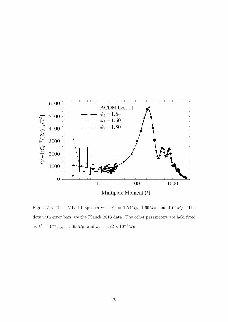
LCDM best fit

Ψi = 1.64

Ψi = 1.60

Ψi = 1.50

10 100 10000

1000

2000

3000

4000

5000

6000

Multipole Moment HL

H+

1LC

T

TH

2ΠL@Μ

K2D

Figure 5.3 The CMB TT spectra with ψi = 1.50MP , 1.60MP , and 1.64MP . The

dots with error bars are the Planck 2013 data. The other parameters are held fixed

as λ′ = 10−9, φi = 3.65MP , and m = 1.22× 10−6MP .

70

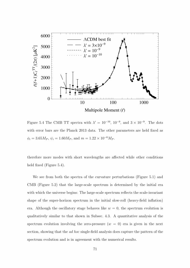
LCDM best fit

Λ' = 3´10-9

Λ' = 10-9

Λ' = 10-10

10 100 10000

1000

2000

3000

4000

5000

6000

Multipole Moment HL

H+

1LC

T

TH

2ΠL@Μ

K2D

Figure 5.4 The CMB TT spectra with λ′ = 10−10, 10−9, and 3 × 10−9. The dots

with error bars are the Planck 2013 data. The other parameters are held fixed as

φi = 3.65MP , ψi = 1.60MP , and m = 1.22× 10−6MP .

therefore more modes with short wavelengths are affected while other conditions

held fixed (Figure 5.4).

We see from both the spectra of the curvature perturbations (Figure 5.1) and

CMB (Figure 5.2) that the large-scale spectrum is determined by the initial era

with which the universe begins: The large-scale spectrum reflects the scale-invariant

shape of the super-horizon spectrum in the initial slow-roll (heavy-field inflation)

era. Although the oscillatory stage behaves like w = 0, the spectrum evolution is

qualitatively similar to that shown in Subsec. 4.3. A quantitative analysis of the

spectrum evolution involving the zero-pressure (w = 0) era is given in the next

section, showing that the ad hoc single-field analysis does capture the pattern of the

spectrum evolution and is in agreement with the numerical results.

71

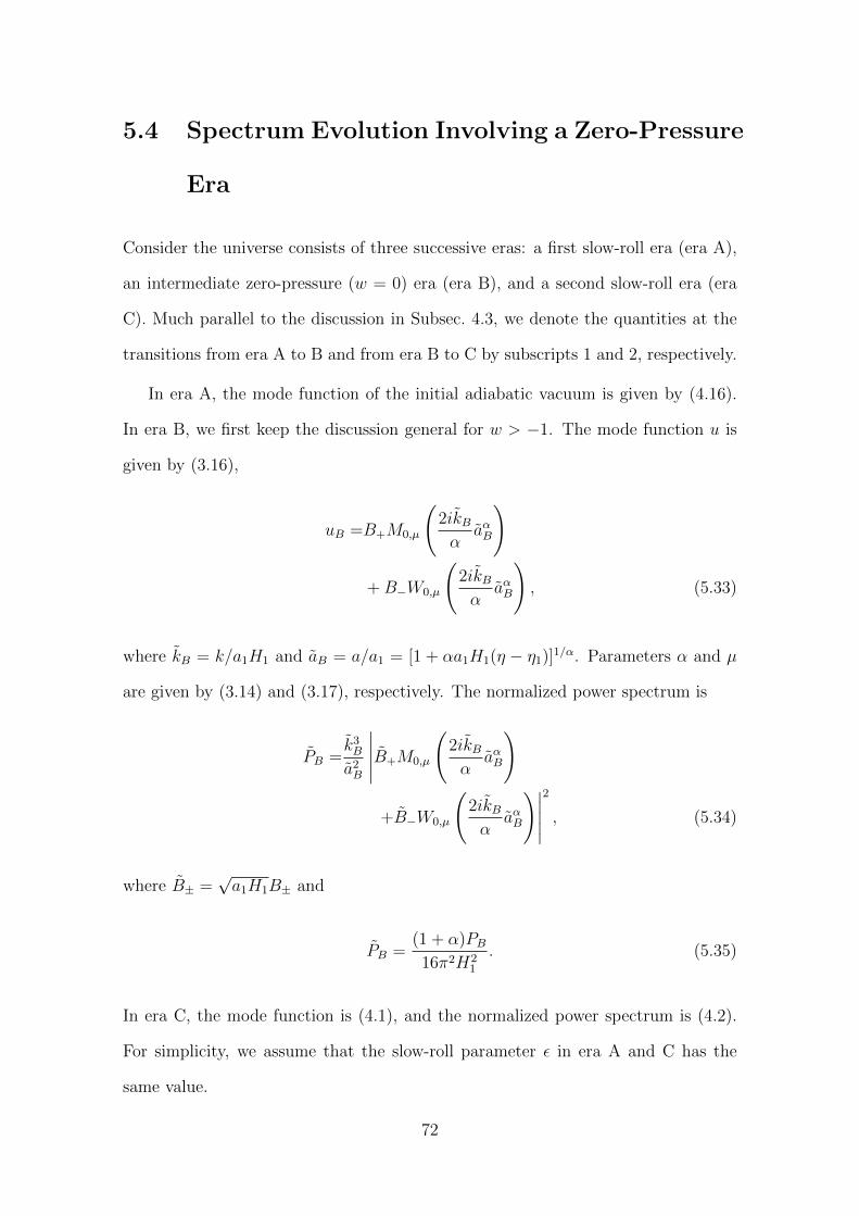
5.4 Spectrum Evolution Involving a Zero-Pressure

Era

Consider the universe consists of three successive eras: a first slow-roll era (era A),

an intermediate zero-pressure (w = 0) era (era B), and a second slow-roll era (era

C). Much parallel to the discussion in Subsec. 4.3, we denote the quantities at the

transitions from era A to B and from era B to C by subscripts 1 and 2, respectively.

In era A, the mode function of the initial adiabatic vacuum is given by (4.16).

In era B, we first keep the discussion general for w > −1. The mode function u is

given by (3.16),

uB =B+M0,µ

(2ikBα

aαB

)

+B−W0,µ

(2ikBα

aαB

), (5.33)

where kB = k/a1H1 and aB = a/a1 = [1 + αa1H1(η − η1)]1/α. Parameters α and µ

are given by (3.14) and (3.17), respectively. The normalized power spectrum is

PB =k3B

a2B

∣∣∣∣∣B+M0,µ

(2ikBα

aαB

)

+B−W0,µ

(2ikBα

aαB

)∣∣∣∣∣2

, (5.34)

where B± =√a1H1B± and

PB =(1 + α)PB16π2H2

1

. (5.35)

In era C, the mode function is (4.1), and the normalized power spectrum is (4.2).

For simplicity, we assume that the slow-roll parameter ε in era A and C has the

same value.

72

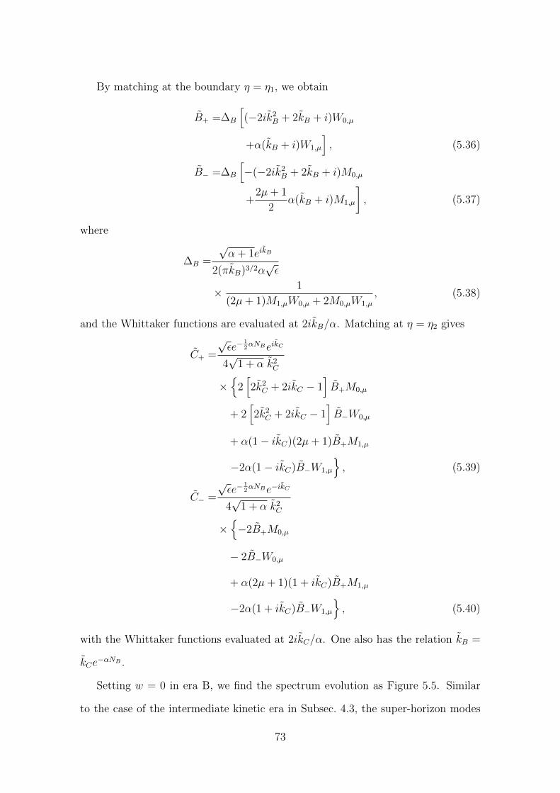
By matching at the boundary η = η1, we obtain

B+ =∆B

[(−2ik2

B + 2kB + i)W0,µ

+α(kB + i)W1,µ

], (5.36)

B− =∆B

[−(−2ik2

B + 2kB + i)M0,µ

+2µ+ 1

2α(kB + i)M1,µ

], (5.37)

where

∆B =

√α + 1eikB

2(πkB)3/2α√ε

× 1

(2µ+ 1)M1,µW0,µ + 2M0,µW1,µ

, (5.38)

and the Whittaker functions are evaluated at 2ikB/α. Matching at η = η2 gives

C+ =

√εe−

12αNBeikC

4√

1 + α k2C

×

2[2k2

C + 2ikC − 1]B+M0,µ

+ 2[2k2

C + 2ikC − 1]B−W0,µ

+ α(1− ikC)(2µ+ 1)B+M1,µ

−2α(1− ikC)B−W1,µ

, (5.39)

C− =

√εe−

12αNBe−ikC

4√

1 + α k2C

×−2B+M0,µ

− 2B−W0,µ

+ α(2µ+ 1)(1 + ikC)B+M1,µ

−2α(1 + ikC)B−W1,µ

, (5.40)

with the Whittaker functions evaluated at 2ikC/α. One also has the relation kB =

kCe−αNB .

Setting w = 0 in era B, we find the spectrum evolution as Figure 5.5. Similar

to the case of the intermediate kinetic era in Subsec. 4.3, the super-horizon modes

73

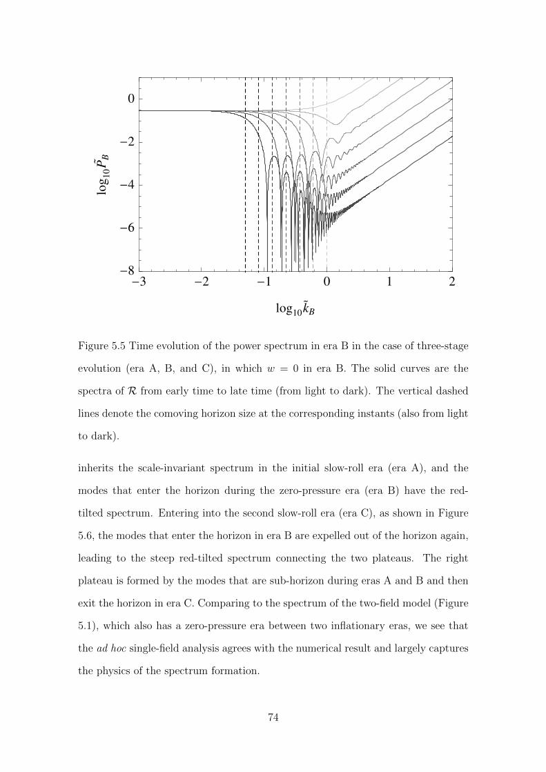
-3 -2 -1 0 1 2-8

-6

-4

-2

0

log10k

B

log

10P

B

Figure 5.5 Time evolution of the power spectrum in era B in the case of three-stage

evolution (era A, B, and C), in which w = 0 in era B. The solid curves are the

spectra of R from early time to late time (from light to dark). The vertical dashed

lines denote the comoving horizon size at the corresponding instants (also from light

to dark).

inherits the scale-invariant spectrum in the initial slow-roll era (era A), and the

modes that enter the horizon during the zero-pressure era (era B) have the red-

tilted spectrum. Entering into the second slow-roll era (era C), as shown in Figure

5.6, the modes that enter the horizon in era B are expelled out of the horizon again,

leading to the steep red-tilted spectrum connecting the two plateaus. The right

plateau is formed by the modes that are sub-horizon during eras A and B and then

exit the horizon in era C. Comparing to the spectrum of the two-field model (Figure

5.1), which also has a zero-pressure era between two inflationary eras, we see that

the ad hoc single-field analysis agrees with the numerical result and largely captures

the physics of the spectrum formation.

74

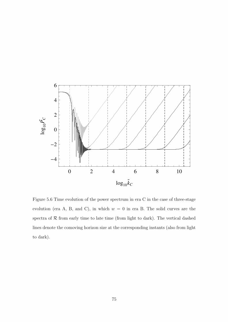
0 2 4 6 8 10

-4

-2

0

2

4

6

log10k

C

log

10P

C

Figure 5.6 Time evolution of the power spectrum in era C in the case of three-stage

evolution (era A, B, and C), in which w = 0 in era B. The solid curves are the

spectra of R from early time to late time (from light to dark). The vertical dashed

lines denote the comoving horizon size at the corresponding instants (also from light

to dark).

75

76

Chapter 6

No-Boundary Wave Function as

the Initial Condition of Inflation

The two candidates we found in the previous analysis—a preinflationary superin-

flation era and a positive-pressure era—both have their difficulties as the realistic

initial condition to the universe. On the one hand, the phantomness of the super-

inflationary era requires a gravitational theory that is self-consistent while breaking

the energy conditions, which is hard to construct. On the other hand, as a decelerat-

ing phase, the positive-pressure era does not have a canonical choice of the vacuum

state such as the Bunch-Davies vacuum. These difficulties may imply that, instead

of struggling in the realm of the semi-classical models, the power suppression can

be more naturally addressed by a quantum gravity theory.

In this chapter, we first describe the Hartle-Hawking no-boundary wave func-

tion, which is a solution to the Wheeler-DeWitt equation that forms the foundation

of quantum gravity, in the minisuperspace model [49, 50]. Especially, we focus on

the background-level solution. We then review the dynamics of the matter field

and metric perturbations introduced by Halliwell and Hawking [56]. By using the

steepest decent approximation, we can calculate the expectation values of perturba-

tions. In the end of this chapter we compute the power spectra of the inflaton field

77

perturbations and show that, with a moderate mass scale, the massive inflaton can

induce the suppression of the long-wavelength spectrum.

6.1 Minisuperspace model

The ADM metric [98] for the homogeneous closed universe is

ds2 = σ2[−(N2 − NiN

i)dλ2 + 2Nidxidλ

+hijdxidxj

], (6.1)

where σ is a constant normalization, and

N = N0(λ), (6.2)

Ni = 0, (6.3)

hij = a2(λ)γij, (6.4)

γijdxidxj = dχ2 + sin2 χ(dθ2 + sin2 θdϕ2) = dΩ2

3. (6.5)

The action for a scalar field in the close universe is

I =1

16π

∫d4x√−gR

+

∫d4x√−g[−1

2∂µΦ∂µΦ− V (Φ)

], (6.6)

where

V (Φ) = V0 +1

2m2Φ2. (6.7)

Defining the variables

φ =

√4π

3Φ, (6.8)

V (Φ) =8πσ2

3V (Φ), (6.9)

78

and integrating over the compact geometry, the action can be expanded as

I[N0, a, φ] =3πσ2

4

∫dλ N0

−a(a′

N0

)2

+ a

+a3

[(φ′

N0

)2

− V (Φ)

], (6.10)

where the primes denote the derivatives against λ. It is convenient to further define

V0 =8πσ2

3V0, (6.11)

m = σm, (6.12)

so that

V = V0 + m2φ2. (6.13)

The no-boundary wave function can be written as the path integral,

Ψ =

∫DaDφDN e−

1~ I[a,φ,N ], (6.14)

where a, φ, and N are the corresponding fields in the Euclidean metric,

ds2 = σ2[N2

0dλ2 + a2dΩ2

3

], (6.15)

obtained from the Lorentzian one by substituting N0 by −iN0 and adding hats to

other fields for clarity. The Euclidean action is taken as I = −iI|N0=−iN0:

I =1

16π

∫d4x√

+gR

+

∫d4x√

+g

[−1

2∂µΦ∂µΦ− V (Φ)

]. (6.16)

After integration, we have

I[N0, a, φ] =3πσ2

4

∫dλ N0

−a(a′

N0

)2

− a

+a3

( φ′

N0

)2

+ V (Φ)

. (6.17)

79

Doing variation with respect to N0, we obtain the Hamiltonian constraint,

˙a2 − 1 + a2[− ˙φ2 + V (Φ)

]= 0, (6.18)

where dots denote derivatives against τ , which is defined by

dτ = N0dλ. (6.19)

Using the steepest descent approximation, the wave function is dominated by the

extreme path (aext(τ), φext(τ)) that satisfies

δI

δa= 0, (6.20)

δI

δφ= 0, (6.21)

which are

¨a+ 2a˙φ2 + aV (Φ) = 0, (6.22)

¨φ+ 3

˙a

a˙φ− 1

2

∂V

∂φ= 0, (6.23)

respectively. Note that the Hamiltonian constraint (6.18) is used when deriving the

equations above.

To solve a(τ), we consider the case in which˙φ2 is negligible, and combine (6.18)

and (6.22) to obtain

a¨a− ˙a2 + 1 = 0. (6.24)

The “no-boundary” boundary condition at τ = 0 sets a(0) = 0. To keep (6.23)

finite, we also require˙φ(0) = 0. Then by the Hamiltonian constraint (6.18) we know

˙a(0) = 1. The only free initial conditions left are the real and imaginary parts of

φ(0).

Equation (6.24) has four solutions,

a(τ) = ± 1

H0

sin [H0(τ − τ0)] , (6.25)

a(τ) = ± 1

H0

sinh [H0(τ − τ0)] . (6.26)

80

For physical solutions we should pick the plus sign. By requiring a(0) = 0 we have

τ0 = 0, and automatically we have consistently ˙a(0) = 1. In order to connect to the

Lorentzian space, which requires a′(τconnect) = 0, the qualified solution is

a(τ) =1

H0

sin(H0τ). (6.27)

The solution connects to the Lorentzian space at τconnect = π/2H0. In Lorentzian

space, we define

dt = N0dλ, (6.28)

therefore dτ = idt. We can then describe the Euclidean trajectory by τ = 0 to

π/2H0, and the Lorentzian one by the complex contour

τ =π

2H0

+ it (6.29)

with t > 0. We then have the Lorentzian solution

a(t) =1

H0

cosh(H0t). (6.30)

6.2 Basis functions on the closed universe

The scalar harmonics are the solutions to

∂i∂iQn(~x) + (n2 − 1)Qn(~x) = 0, (n = 1, 2, 3 . . . ). (6.31)

and each Qn(~x) is a finite sum over l and m (with l = 0, 1, . . . , n − 1 and m =

−l,−l + 1, . . . , l) like the familiar spherical harmonics Ylm(θ, ϕ) on S2. We write

Qn(~x) as

Qnlm(χ, θ, ϕ) = Πnl(χ)Ylm(θ, ϕ). (6.32)

In closed universe, the Laplacian is

~∇2 =1

sin2 χ

[sin2 χ

∂2

∂χ2+ 2 sinχ cosχ

∂

∂χ+

1

sin θ

∂

∂θ

(sin θ

∂

∂θ

)+

1

sin2 θ

∂2

∂ϕ2

].

(6.33)

81

One can recognize that the last two terms in the bracket are actually the operator

of spherical harmonics. The Fock harmonics Πnl satisfy

d2Πnl

dχ2+ 2 cotχ

dΠnl

dχ+

[(n2 − 1)− l(l + 1)

sin2 χ

]Πnl = 0. (6.34)

The solutions are

Πnl(χ) =

√2

nπ

(n− l − 1)!

(n+ l)!(sinχ)l

(d

d cosχ

)l+1

cos(nχ), (6.35)

Ylm(θ, ϕ) =

√2l + 1

4π

(l −m)!

(l +m)!Pml (cos θ)eimϕ, (6.36)

with orthonormal inner products∫ π

0

dχ

∫ π

0

dθ

∫ 2π

0

dϕ sin2 χ sin θ [Πn′l′(χ)Yl′m′(θ, ϕ)]∗ [Πnl(χ)Ylm(θ, ϕ)] = δnn′δll′δmm′ .

(6.37)

Similar definitions exist for other basis functions.

6.3 Perturbation spectrum from the wave func-

tion

The perturbations to the spatial part of the metric in the S3 × R closed universe

can be organized as

hij = a2γij,

γij = γij + εij, (6.38)

where εij denotes

εij =∑n,l,m

[√6qnlm

1

3γijQnlm +

√6bnlm(Pij)nlm

+√

2conlm(Soij)nlm +√

2cenlm(Seij)nlm

+2donlm(Goij)nlm + 2denlm(Ge

ij)nlm], (6.39)

82

and

Pij =1

n2 − 1∇i∇jQ+

1

3γijQ. (6.40)

Here the covariant derivatives are with respect to γij. The first, second, and third

lines of (6.39) denote the scalar, vector, and tensor perturbations, respectively. Sup-

pressing the spherical coordinate indices, n, l, m, the coefficients, q, b, co, ce, do, de,

are time dependent, while the basis, Q, Pij, Soij, S

eij, G

oij, G

eij, are space dependent.

The perturbations to the lapse and the shift functions are

N = N0

[1 +

∑n,l,m

1√6gnlmQnlm

], (6.41)

Ni = a∑n,l,m

[1√6knlm(Pi)nlm +

√2jnlm(Si)nlm

], (6.42)

where

Pi =1

n2 − 1∇iQ. (6.43)

Finally, the perturbation to the scalar field is

Φ =

√3

4πφ+

∑n,l,m

√3π

2fnlmQnlm. (6.44)

Among the perturbations, q, b, g, k, and f are the scalar ones, j, co and ce are the

vector ones, and do and de are the tensor ones.

The action can be expanded around the background fields to the second order

as the sum of the eigenmodes [56],

I = I0(a, φ, N0)

+∑n,l,m

Inlm(a, φ, N0; qnlm, . . . , knlm). (6.45)

Choosing the gauge in which qnlm = bnlm = 0, the constraint equations can be

obtained by variating the quadratic part of the perturbation action with respect to

83

gnlm and knlm,

gnlm = 3(n2 − 1)Hφfnlm + φfnlm + m2φfnlm

(n2 − 4)H2 + 3φ2, (6.46)

knlm = 3(n2 − 1)N0a

× Hφfnlm +Hm2φfnlm − 3φ(−H2 + φ2)fnlm

(n2 − 4)H2 + 3φ2. (6.47)

Here the dots denote derivatives against the Lorentzian time t. The equation of

motion for fnlm can be obtained by the variation with respect to fnlm,

fnlm + 3Hfnlm +

(m2 +

n2 − 1

a2

)fnlm

= −2m2φgnlm + φgnlm −φknlmN0a

. (6.48)

The amplitude of the perturbations of the scalar field, δΦ, can be obtained

through calculating the expectation value with the no-boundary wave function, fo-

cusing on the part relevant for fnlm. Using the steepest descent approximation,

the Euclidean action I in the wave function receives contributions mostly from the

solution to the equations of motion, evaluated to be

I ≈ a3

2iN

(fnlm

dfnlmdτ− dφ

dτgnlmfnlm

)=

1

2a3

(fnlm

dfnlmdt− dφ

dtgnlmfnlm

). (6.49)

We therefore have

Ψ[fnlm] ≈ Bnlm exp

[−1

2a3(fnlmfnlm − φgnlmfnlm

)], (6.50)

where the dots denote derivatives against t. The normalization can be fixed by

requiring

|Bnlm|2∫ ∞−∞

dfnlm∣∣∣∣exp

[−1


)]∣∣∣∣2 = 1. (6.51)

84

The expectation of the field perturbations averaged over the space is given by

〈δΦ2(t, ~x)〉 =1

2π2

∫dχdθdϕ sin2 χ sin θ

× 3π

2

∑nlm

∑n′l′m′

〈fnlmfn′l′m′〉QnlmQn′l′m′

=3

4π

∑nlm

〈f 2nlm〉, (6.52)

where

〈f 2nlm〉 = |Bnlm|2

∫ ∞−∞

dfnlm

f 2nlm

∣∣∣∣exp

[−1


)]∣∣∣∣2 . (6.53)

Defining the power spectrum, P (n), as

〈δΦ2(t, ~x)〉 =∑n

1

nP (n), (6.54)

with l and m summed over, we then find

P (n) =3n

4π

∑l,m

〈f 2nlm〉. (6.55)

Note that if 〈f 2nlm〉 depends only on n, the summation over l and m can be imme-

diately carried out, leaving

P (n) =3n3

4π〈f 2n〉. (6.56)

To evaluate the expectation value 〈f 2nlm〉, we adopt the proposal of [57]. We

replace fnlm by a combination of the canonical variable fnlm and its c-number value

fnlm,

fnlm →˙fnlm

fnlmfnlm. (6.57)

When φ or the metric perturbations gnlm are negligible, the wave function is then

Ψ[fnlm] = Bnlm exp

(−a

3 ˙fnlm

2fnlmf 2nlm

). (6.58)

85

The normalization is evaluated as

|Bnlm|2 =

√√√√a3 ˙fnlm

πfnlm. (6.59)

The expectation value can then be found to be

〈f 2nlm〉 =

fnlm

2a3 ˙fnlm. (6.60)

6.4 Effect of mass on the power spectrum

In the Euclidean space, we consider the scale factor solution (6.27) and a constant

scalar field in the background. Neglecting the metric perturbations gn (we suppress

the indices l and m in this section, since the equation of motion does not depend on

them), we calculate the field perturbations fn (we ignore the tilde that denotes the

c-number solution wherever no confusion arises) by numerically solving the equation

of motion

d2fndτ 2

+ 3H0 cot(H0τ)dfndτ−[m2 +

(n2 − 1)H20

sin2(H0τ)

]fn = 0, (6.61)

where we use the hat to emphasize that it is the solution in the Euclidean space.

In order to keep equation (6.61) finite, we require that both fn(τ) and f ′n(τ) vanish

at τ = 0. More precisely, we adopt the following ansatz as the initial condition for

numerical calculations:

fn(τi) =1

2ετ 2i , (6.62)

˙fn(τi) = ετi, (6.63)

where τi 1 is the initial Euclidean time from which we start to integrate the dif-

ferential equations, and ε is an arbitrary parameter. Note that since the expectation

value 〈f 2n〉 depends only on the ratio fn/

˙fn, the power spectrum is independent of

the choice of ε. In our numerical calculation, we set τi = 10−4 and ε = 1, and evolve

the Euclidean system from τi to τf = π/2H0.

86

In the Lorentzian spacetime, we use the analytical solution (6.30) for the scale

factor and a constant scalar field in the background to model the slow-roll inflation.

The equation of motion for the field perturbation reads

d2fndt2

+ 3H0 tanh(H0t)dfndt

+

[m2 +

(n2 − 1)H20

cosh2(H0t)

]fn = 0. (6.64)

The boundary conditions connecting the Euclidean and Lorentzian solutions are the

Cauchy-Riemann conditions [51, 52, 53, 54, 55]

Ref(ti) = Ref(τf ), (6.65)

Imf(ti) = Imf(τf ), (6.66)

Ref(ti) = −Im ˙f(τf ), (6.67)

Imf(ti) = Re ˙f(τf ), (6.68)

where we set ti = 0 to be the initial time of integration in the Lorentzian space. We

then solve the system from ti to the horizon-exit time,

texit =1

H0

sinh−1 n, (6.69)

for mode n. Note that for each mode, the expectation value (6.60), hence the power

spectrum (6.55), is evaluated at its horizon-exit time.1

The Hubble parameter in the Lorentzian space is

H(t) = H0 tanh(H0t). (6.70)

Therefore H0 corresponds to the Hubble constant during the exponentially growing

period. To fix the value of H0, we consider the Hamiltonian constraint in Lorentzian

1The power spectrum in general does not conserve at super-horizon scales, given that we are

calculating the spectrum of the inflaton field perturbations in a closed FLRW universe, adopting the

wave function interpretation to deduce the expectation values of the perturbations. The relation

between this formulation and the approach of traditional quantum field theory still requires further

clarification, which we leave to the future works.

87

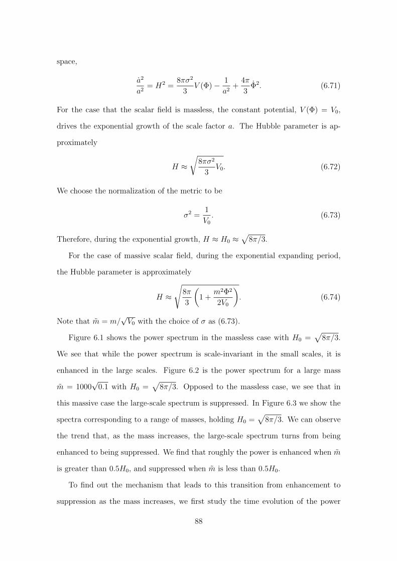
space,

a2

a2= H2 =

8πσ2

3V (Φ)− 1

a2+

4π

3Φ2. (6.71)

For the case that the scalar field is massless, the constant potential, V (Φ) = V0,

drives the exponential growth of the scale factor a. The Hubble parameter is ap-

proximately

H ≈√

8πσ2

3V0. (6.72)

We choose the normalization of the metric to be

σ2 =1

V0

. (6.73)

Therefore, during the exponential growth, H ≈ H0 ≈√

8π/3.

For the case of massive scalar field, during the exponential expanding period,

the Hubble parameter is approximately

H ≈

√8π

3

(1 +

m2Φ2

2V0

). (6.74)

Note that m = m/√V0 with the choice of σ as (6.73).

Figure 6.1 shows the power spectrum in the massless case with H0 =√

8π/3.

We see that while the power spectrum is scale-invariant in the small scales, it is

enhanced in the large scales. Figure 6.2 is the power spectrum for a large mass

m = 1000√

0.1 with H0 =√

8π/3. Opposed to the massless case, we see that in

this massive case the large-scale spectrum is suppressed. In Figure 6.3 we show the

spectra corresponding to a range of masses, holding H0 =√

8π/3. We can observe

the trend that, as the mass increases, the large-scale spectrum turns from being

enhanced to being suppressed. We find that roughly the power is enhanced when m

is greater than 0.5H0, and suppressed when m is less than 0.5H0.

To find out the mechanism that leads to this transition from enhancement to

suppression as the mass increases, we first study the time evolution of the power

88

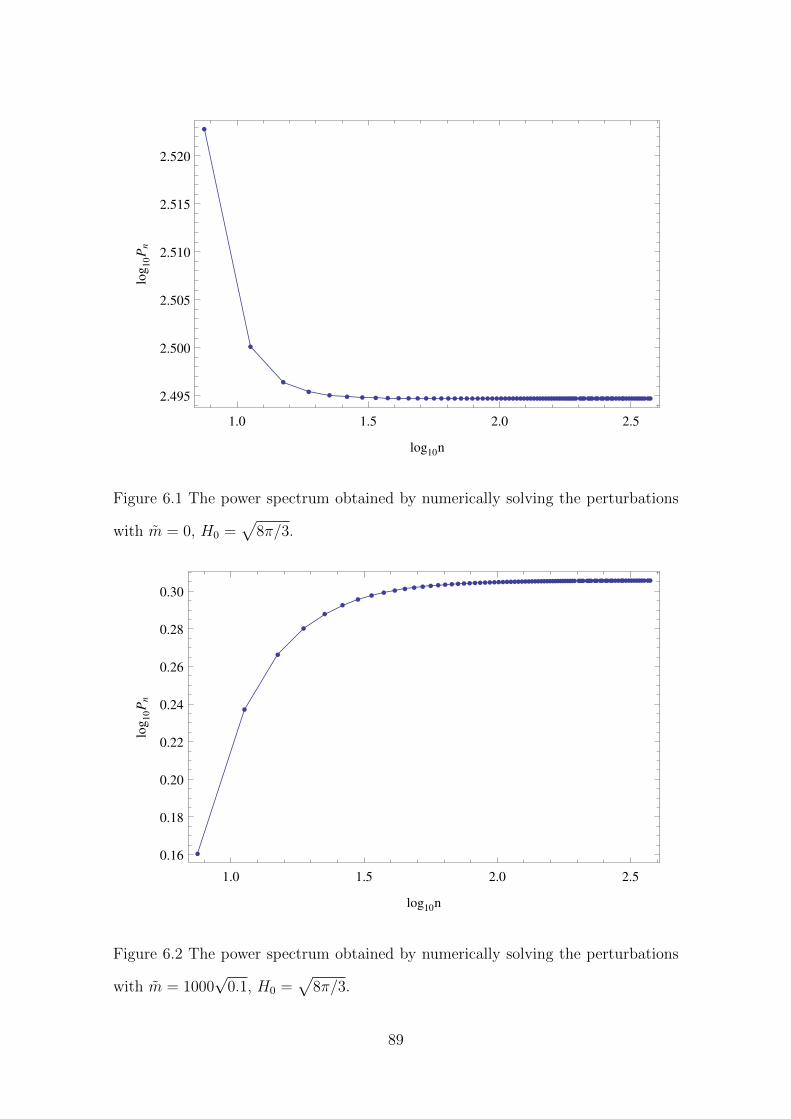
1.0 1.5 2.0 2.5

2.495

2.500

2.505

2.510

2.515

2.520

log10n

log

10P

n

Figure 6.1 The power spectrum obtained by numerically solving the perturbations

with m = 0, H0 =√

8π/3.

1.0 1.5 2.0 2.5

0.16

0.18

0.20

0.22

0.24

0.26

0.28

0.30

log10n

log

10P

n


with m = 1000√

0.1, H0 =√

8π/3.

89

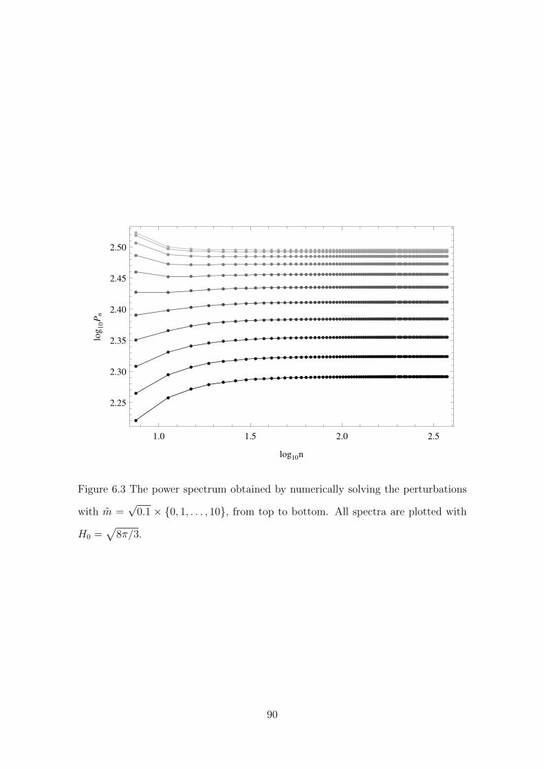
1.0 1.5 2.0 2.5

2.25

2.30

2.35

2.40

2.45

2.50

log10n

log

10P

n


with m =√

0.1 × 0, 1, . . . , 10, from top to bottom. All spectra are plotted with

H0 =√

8π/3.

90

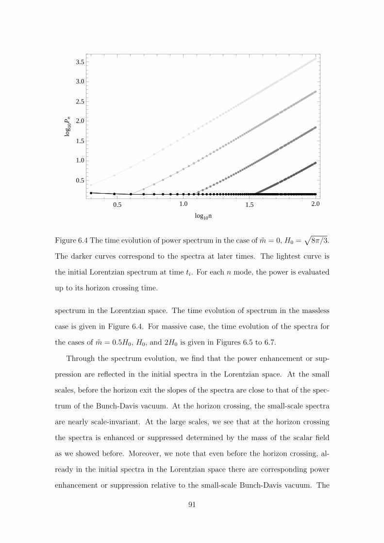
0.5 1.0 1.5 2.0

0.5

1.0

1.5

2.0

2.5

3.0

3.5

log10n

log

10P

n

Figure 6.4 The time evolution of power spectrum in the case of m = 0, H0 =√

8π/3.

The darker curves correspond to the spectra at later times. The lightest curve is

the initial Lorentzian spectrum at time ti. For each n mode, the power is evaluated

up to its horizon crossing time.

spectrum in the Lorentzian space. The time evolution of spectrum in the massless

case is given in Figure 6.4. For massive case, the time evolution of the spectra for

the cases of m = 0.5H0, H0, and 2H0 is given in Figures 6.5 to 6.7.

Through the spectrum evolution, we find that the power enhancement or sup-

pression are reflected in the initial spectra in the Lorentzian space. At the small

scales, before the horizon exit the slopes of the spectra are close to that of the spec-

trum of the Bunch-Davis vacuum. At the horizon crossing, the small-scale spectra

are nearly scale-invariant. At the large scales, we see that at the horizon crossing

the spectra is enhanced or suppressed determined by the mass of the scalar field

as we showed before. Moreover, we note that even before the horizon crossing, al-

ready in the initial spectra in the Lorentzian space there are corresponding power

enhancement or suppression relative to the small-scale Bunch-Davis vacuum. The

91

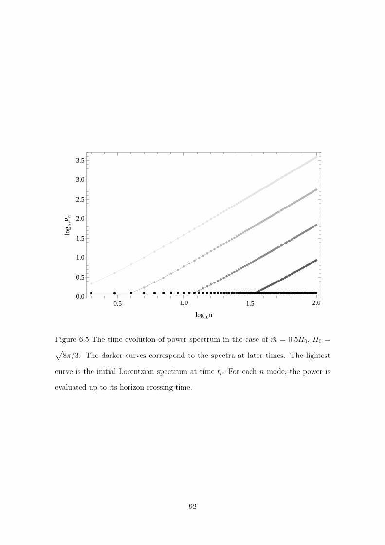
0.5 1.0 1.5 2.00.0

0.5

1.0

1.5

2.0

2.5

3.0

3.5

log10n

log

10P

n

Figure 6.5 The time evolution of power spectrum in the case of m = 0.5H0, H0 =√8π/3. The darker curves correspond to the spectra at later times. The lightest

curve is the initial Lorentzian spectrum at time ti. For each n mode, the power is

evaluated up to its horizon crossing time.

92

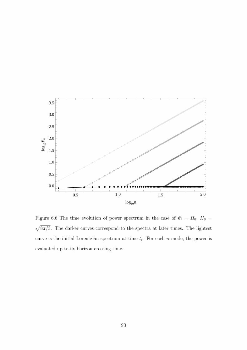
0.5 1.0 1.5 2.0

0.0

0.5

1.0

1.5

2.0

2.5

3.0

3.5

log10n

log

10P

n

Figure 6.6 The time evolution of power spectrum in the case of m = H0, H0 =√8π/3. The darker curves correspond to the spectra at later times. The lightest



93

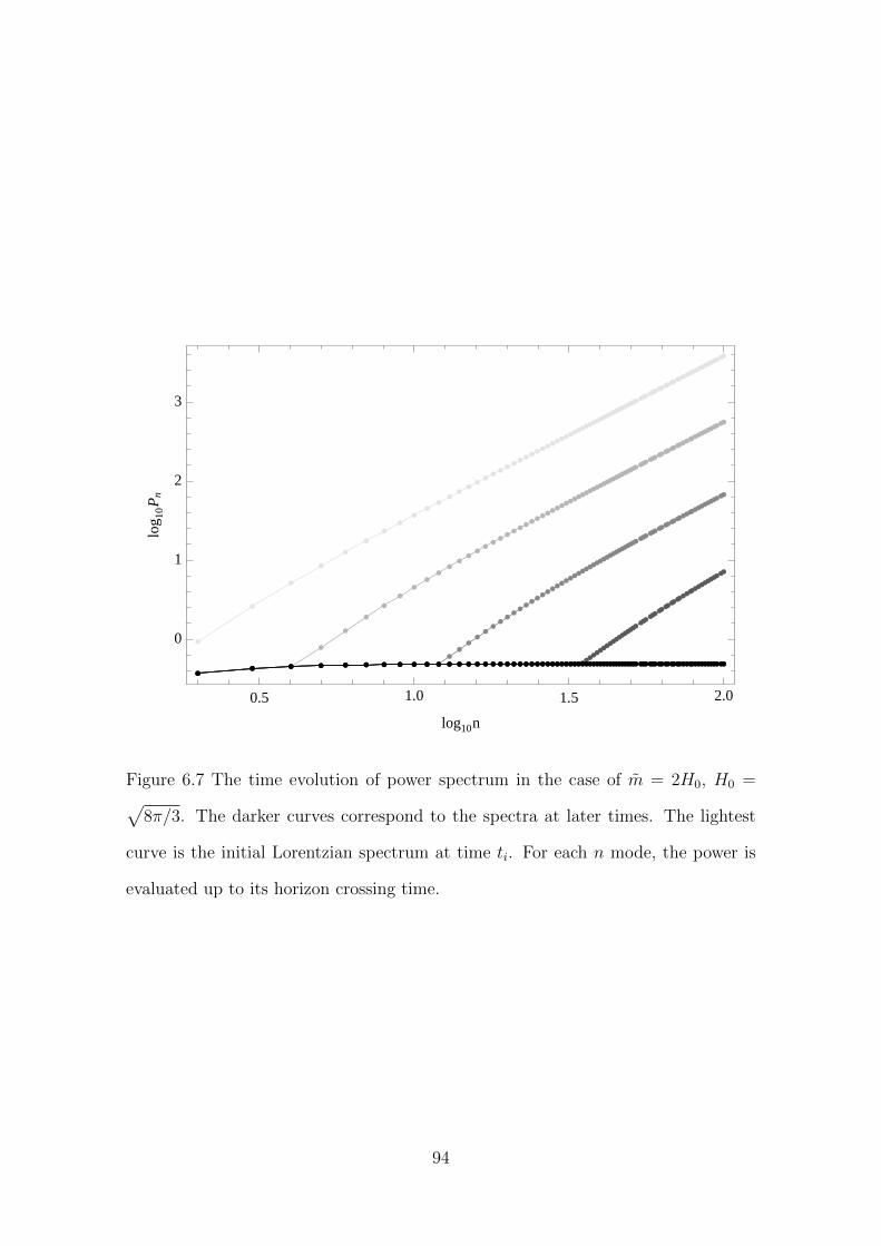
0.5 1.0 1.5 2.0

0

1

2

3

log10n

log

10P

n

Figure 6.7 The time evolution of power spectrum in the case of m = 2H0, H0 =√8π/3. The darker curves correspond to the spectra at later times. The lightest



94

origin of the power enhancement or suppression therefore lies on the Lorentzian

initial condition, or, equivalently, on the Euclidean final spectrum.

To find out the effect of mass on the Euclidean final spectrum, we note that the

Euclidean equation of motion (6.61) can also be analytically solved, yielding the

solution

fn(τ) = AP nν [cos(H0τ)]

sin(H0τ), (6.75)

where A is an overall coefficient that has no effect on the final Euclidean spectrum,

ν =−1 +

√9− 4m2/H2

0

2, (6.76)

and we have picked the solution that is consistent with the no-boundary initial

condition. When m2/H20 > 9/4, ν and fn(τ) become complex. The power spectrum

at the beginning of the Lorentzian time can be evaluated using the Euclidean solution

at τ = π/2H0 through the boundary conditions. When evaluating the ratio fn/˙fn

with complex fn, we interpret it as the amplitude |fn/ ˙fn|. We then have the initial

power spectrum in the Lorentzian space as

P (n) =3n3H2

0

8π

∣∣∣∣ P nν (0)

P nν′(0)

∣∣∣∣ . (6.77)

In the large-mass limit, we can intuitively understand the power suppression of the

initial power spectrum induced by the mass term in the following way. In such a

limit, the solution to the equation of motion (6.61) roughly consists of an expo-

nentially growing mode, exp(mτ), and an exponentially decaying mode, exp(−mτ).

Hence, the amplitude |fn/ ˙fn| is roughly of the order of 1/m, which is suppressed by

m = m/√V0. Note that the large-mass limit actually lies beyond the linear regime

of perturbations, and the purpose of considering it is only to provide an intuitive

understanding. As shown in Figure 6.3, the long-wavelength spectrum is already

suppressed as m2/H20 is as small as roughly 0.1

√6/√

8π/3 ≈ 0.43. Therefore, it

only requires a moderate mass to induce the effect of suppression.

95

96

Chapter 7

Conclusions and Discussions

In this thesis we explore the initial conditions to the inflationary universe using the

long-wavelength suppression of the CMB spectrum as an important observational

clue. We start by considering the toy model to the preinflationary era that consists of

the NFTD of two kinds: (i) a NFDW that induces an accelerating rate smaller than

that of the standard slow-roll inflation, and (ii) a NFCS that describes a universe

expanding in a constant rate. We model such a matter content for the very early

universe as a kind of the generalized Chaplygin gas described by Eq. (2.18) (see also

Eq. (2.1)), which gives a smooth transition from a NFTD dominated era to a de

Sitter-like phase or a power-law inflationary era. We constrain our model using the

WMAP7 data for the power spectrum of the scalar perturbations, Ps = 2.45×10−9,

and the spectral index, ns = 0.963, at the pivot scale, k0 = 0.002 Mpc−1 [77]. After

fixing the parameters of the model and imposing the approximate initial vacuum

states for the perturbations, we obtain the curvature power spectra for the cases of a

NFDW and a NFCS, as shown in Figures 2.6 and 2.7. The most important feature of

the spectra is the drop of the power for the long-wavelength modes with k ≤ 0.002

Mpc−1. Nevertheless, through a more detailed and systematic analysis presented

later, the initial vacua are found to have different structures from the approximated

ones used here. In particular, we will see that for the case of the preinflationary

97

NFDW dominated era, the large-scale spectrum is actually enhanced, rather than

suppressed.

We then systematically investigate the power spectrum in the general background

geometry. We study the curvature perturbations of a scalar field in the FLRW

universe parameterized by the equation of state parameter w, and find that the

large-scale spectrum at the end of inflation reflects the super-horizon spectrum of

the initial state. We show that if the universe begins in the superinflation era (w <

−1) or that with positive pressure (w > 0), the large-scale curvature perturbation

spectrum is suppressed due to the blue-tilted super-horizon spectrum in the initial

era. We first find the scaling relation of the super-horizon spectrum for a scalar

field in the FLRW background with constant equation of state. At the large scales,

the spectrum is blue-tilted for positive-pressure (w > 0) or superinflation (w < −1)

era, and red-tilted for the era with −1 < w < 0, except the singular case with w =

−1/3. In the slow-roll (w ' −1) and zero-pressure (w = 0) background, the super-

horizon spectrum is scale-invariant. We also point out that the conclusions are drawn

from assuming the mode function approaches the Minkowski limit at small scales.

Although being natural in the accelerating universe, this assumption becomes a

posteriori in the decelerating universe since the sub-horizon modes are evolved from

the super-horizon modes, which are initially across causally disconnected regions

before entering the horizon.

We develop the method of spectrum evolution to analyze how the expansion of

the background geometry transforms the initial spectrum in the preinflationary era

into the super-horizon spectrum in the inflationary era. By analyzing three scenar-

ios: a single slow-roll era, a slow-roll era preceded by a kinetic era, and two successive

slow-roll eras connected by a kinetic era, we show the following two facts. First, the

large-scale power suppression in the model with a single preinflation kinetic era

stems from the blue-tilted super-horizon spectrum of the initial kinetic era. Second,

98

the additional slow-roll era preceding the kinetic era changes the super-horizon ini-

tial spectrum, so the large-scale power is enhanced, rather than suppressed. These

results show that the large-scale spectrum depends sensitively on the initial vacuum.

In the universe beginning with the positive-pressure era, as we pointed out earlier,

the super-horizon modes are initially across causally disconnected regions, and the

well-motivated assumption on the initial state is still lacking. Some investigations

about the effect of the different initial vacuum on the spectrum have been carried

out in the literature [31, 32, 33, 34]. We also explore the case that is free from the

acausal issue: a superinflation era preceding the slow-roll era, and show that the

large-scale spectrum is suppressed due to the initially blue-tilted spectrum in the

superinflation era.

To show that the pattern of evolution we obtain through the single-field analysis

also applies to the two-field systems, we calculate the curvature perturbation and

CMB spectra of a two-stage inflation model from the given two-field potential. We

show that the large-scale power is enhanced due to the initial spectrum set in the first

accelerating era, and the effect of the intermediate decelerating era on the spectrum

is connecting the two plateaus generated in the two accelerating eras, which agrees

with the picture obtained through the ad hoc single-field analysis.

In view of the shortcomings of the positive-pressure era and the superinflation

era as consistent initial conditions to the universe, we explore other possibilities pro-

vided by the quantum gravitational theory. Particularly, we investigate the power

spectrum of perturbations with the no-boundary wave function [47] as the initial con-

dition of the inflationary universe. We have relied on very conservative approaches,

including the canonical quantization [48], the Euclidean path integral approach and

the steepest descent approximation [47], and the use of instantons at the background

as well as perturbation levels [56], which are consistent with traditional techniques of

quantum field theory in several regimes [99]. We find that the inflationary universe is

99

approximately scale-invariant at the short-wavelength scales, while the power spec-

trum of the pure de Sitter space is enhanced at the long-wavelength scales. We

also find that the power spectrum can be either enhanced or suppressed due to the

detailed choice of the potential; for example, the mass term of the inflaton field. In

particular, as long as the inflaton is moderately massive, the long-wavelength spec-

trum is suppressed. This opens a possibility that the power suppression is indeed a

hint to that our universe starts from an instanton with a massive inflaton field that

approximates the Hartle-Hawking wave function.

This line of exploration definitely needs more work. It will be interesting to

see more detailed calculations for other realistic inflationary scenarios; e.g., the

Starobinsky-type inflation models [100]. Also, we investigated for compact and ho-

mogeneous instantons, but there are other instantons that also explain the origin of

our universe; e.g., the Coleman-De Luccia instantons [101] or the Euclidean worm-

holes [102, 103, 104]. Another brave question is: what is the relation between the

big bounce model of the loop quantum cosmology [46] and the Hartle-Hawking wave

function [47]? Both approaches explain the power suppression, but it is yet unclear

which one is more suitable as the model of the beginning of our universe. We leave

these interesting issues as future research topics.

100

Bibliography

[1] G. F. Smoot et al., Structure in the COBE differential microwave radiometer

first-year maps, Astrophys. J. 396 (Sep, 1992) L1–L5.

[2] M. Tegmark, The angular power spectrum of the four-year COBE data,

Astrophys. J. 464 (1996) L35.

[3] C. L. Bennett, D. Larson, J. L. Weiland, N. Jarosik, G. Hinshaw,

N. Odegard, K. M. Smith, R. S. Hill, B. Gold, M. Halpern, E. Komatsu,

M. R. Nolta, L. Page, D. N. Spergel, E. Wollack, J. Dunkley, A. Kogut,

M. Limon, S. S. Meyer, G. S. Tucker, and E. L. Wright, Nine-year Wilkinson

Microwave Anisotropy Probe (WMAP) observations: Final maps and results,

Astrophys. J. Suppl. Ser. 208 (2013), no. 2 20.

[4] Planck Collaboration, Planck 2013 results. XV. CMB power spectra and

likelihood, Astron. Astrophys. 571 (2014) A15.

[5] Planck Collaboration, Planck 2015 results. XI. CMB power spectra,

likelihoods, and robustness of parameters, Astron. Astrophys. 594 (2016) A11.

[6] C. R. Contaldi, M. Peloso, L. Kofman, and A. Linde, Suppressing the lower

multipoles in the CMB anisotropies, J. Cosmol. Astropart. Phys. 07 (2003)

002.

[7] I.-C. Wang and K.-W. Ng, Effects of a preinflation radiation-dominated

epoch to CMB anisotropy, Phys. Rev. D 77 (Apr, 2008) 083501.

101

[8] F. Scardigli, C. Gruber, and P. Chen, Black hole remnants in the early

universe, Phys. Rev. D 83 (Mar, 2011) 063507.

[9] M. Bouhmadi-Lopez, P. Chen, Y.-C. Huang, and Y.-H. Lin, Slow-roll

inflation preceded by a topological defect phase a la Chaplygin gas, Phys. Rev.

D 87 (May, 2013) 103513.

[10] S. Kouwn, O.-K. Kwon, and P. Oh, Large scale suppression of scalar power

on a spatial condensation, Phys. Rev. D 91 (Mar, 2015) 063521.

[11] R. K. Jain, P. Chingangbam, J.-O. Gong, L. Sriramkumar, and

T. Souradeep, Punctuated inflation and the low CMB multipoles, J. Cosmol.

Astropart. Phys. 01 (2009) 009.

[12] E. Dudas, N. Kitazawa, S. Patil, and A. Sagnotti, CMB imprints of a

pre-inflationary climbing phase, J. Cosmol. Astropart. Phys. 05 (2012) 012.

[13] M. H. Namjoo, H. Firouzjahi, and M. Sasaki, Multiple inflationary stages

with varying equation of state, J. Cosmol. Astropart. Phys. 2012 (2012),

no. 12 018. arXiv:1207.3638.

[14] J. White, Y.-l. Zhang, and M. Sasaki, Scalar suppression on large scales in

open inflation, Phys. Rev. D 90 (Oct, 2014) 083517.

[15] T. Biswas and A. Mazumdar, Super-inflation, non-singular bounce, and low

multipoles, Class. Quant. Grav. 31 (2014), no. 2 025019.

[16] S. Endlich, A. Nicolis, and J. Wang, Solid inflation, J. Cosmol. Astropart.

Phys. 10 (2013) 011.

[17] D. Polarski and A. Starobinsky, Spectra of perturbations produced by double

inflation with an intermediate matter-dominated stage, Nucl. Phys. B 385

(1992) 623.

102

[18] A. Ashoorioon and A. Krause, Power spectrum and signatures for cascade

inflation, arXiv:hep-th/0607001.

[19] A. Ashoorioon, A. Krause, and K. Turzynski, Energy transfer in multi field

inflation and cosmological perturbations, J. Cosmol. Astropart. Phys. 02

(2009) 014.

[20] D. Yamauchi, A. Linde, A. Naruko, M. Sasaki, and T. Tanaka, Open

inflation in the landscape, Phys. Rev. D 84 (Aug, 2011) 043513.

[21] A. Linde, Hybrid inflation, Phys. Rev. D 49 (Jan, 1994) 748–754.

[22] M. Bucher and D. Spergel, Is the dark matter a solid?, Phys. Rev. D 60 (Jul,

1999) 043505.

[23] R. A. Battye, M. Bucher, and D. Spergel, Domain wall dominated universes,

arXiv:astro-ph/9908047.

[24] D. Spergel and U.-L. Pen, Cosmology in a string-dominated universe,

Astrophys. J. Lett. 491 (1997), no. 2 L67.

[25] M. Bouhmadi-Lopez, P. F. Gonzalez-Dıaz, and A. Zhuk, On new

gravitational instantons describing creation of brane worlds, Class. Quant.

Grav. 19 (2002) 4863.

[26] M. Bouhmadi-Lopez, P. F. Gonzalez-Dıaz, and A. Zhuk, Topological defect

brane world models, Grav. Cosmol. 8 (2002) 285.

[27] A. Vilenkin and E. Shellard, Cosmic Strings and Other Topological Defects.

Cambridge University Press, 2000.

[28] H. Kubotani, The domain wall network of explicitly broken O(N) model,

Prog. Theor. Phys. 87 (1992), no. 2 387.

103

[29] Y. Nambu, H. Ishihara, H. Gouda, and H. Sugiyama, Anisotropies of the

cosmic background radiation by domain wall networks, Astrophys. J. Lett.

373 (1991) L35.

[30] P. Chen and Y.-H. Lin, What initial condition of inflation would suppress the

large-scale CMB spectrum?, Phys. Rev. D 93 (Jan, 2016) 023503.

[31] L. Sriramkumar and T. Padmanabhan, Initial state of matter fields and

trans-Planckian physics: Can CMB observations disentangle the two?, Phys.

Rev. D 71 (May, 2005) 103512.

[32] D. Boyanovsky, H. J. de Vega, and N. G. Sanchez, CMB quadrupole

suppression. I. initial conditions of inflationary perturbations, Phys. Rev. D

74 (Dec, 2006) 123006.

[33] R. Holman and A. J. Tolley, Enhanced non-gaussianity from excited initial

states, J. Cosmol. Astropart. Phys. 05 (2008) 001.

[34] I. Agullo and L. Parker, Non-gaussianities and the stimulated creation of

quanta in the inflationary universe, Phys. Rev. D 83 (Mar, 2011) 063526.

[35] V. Mukhanov and M. Zelnihov, What kinds of perturbation spectra can be

produced by inflation?, Phys. Lett. B 263 (1991), no. 2 169 – 175.

[36] S. Tsujikawa, P. Singh, and R. Maartens, Loop quantum gravity effects on

inflation and the CMB, Class. Quant. Grav. 21 (2004), no. 24 5767.

[37] A. Ashtekar and D. Sloan, Loop quantum cosmology and slow roll inflation,

Phys. Lett. B 694 (2010), no. 2 108 – 112.

[38] G. Domenech and M. Sasaki, Conformal frame dependence of inflation, J.

Cosmol. Astropart. Phys. 04 (2015) 022.

104

[39] Y.-S. Piao and Y.-Z. Zhang, Phantom inflation and primordial perturbation

spectrum, Phys. Rev. D 70 (Sep, 2004) 063513.

[40] M. Baldi, F. Finelli, and S. Matarrese, Inflation with violation of the null

energy condition, Phys. Rev. D 72 (Oct, 2005) 083504.

[41] S. M. Carroll, M. Hoffman, and M. Trodden, Can the dark energy

equation-of-state parameter w be less than −1?, Phys. Rev. D 68 (Jul, 2003)

023509.

[42] J. M. Cline, S. Jeon, and G. D. Moore, The phantom menaced: Constraints

on low-energy effective ghosts, Phys. Rev. D 70 (Aug, 2004) 043543.

[43] A. Lewis, A. Challinor, and A. Lasenby, Efficient computation of CMB

anisotropies in closed frw models, Astrophys. J. 538 (2000) 473–476.

[44] A. Lewis and A. Challinor, Code for anisotropies in the microwave

background, http://camb.info/ Oct.

[45] T. S. Bunch and P. C. W. Davies, Quantum field theory in de Sitter space:

Renormalization by point-splitting, Proceedings of the Royal Society of

London. A. Mathematical and Physical Sciences 360 (1978), no. 1700

117–134.

[46] A. Ashtekar and A. Barrau, Loop quantum cosmology: From pre-inflationary

dynamics to observations, Class. Quant. Grav. 32 (2015), no. 23 234001.

arXiv:1504.07559 [gr-qc].

[47] J. B. Hartle and S. W. Hawking, Wave function of the universe, Phys. Rev.

D 28 (1983) 2960.

[48] B. S. DeWitt, Quantum theory of gravity. I. the canonical theory, Phys. Rev.

160 (Aug, 1967) 1113–1148.

105

[49] J. B. Hartle, S. W. Hawking, and T. Hertog, The no-boundary measure of

the universe, Phys. Rev. Lett. 100 (2008) 201301.

[50] J. B. Hartle, S. W. Hawking, and T. Hertog, Classical universes of the

no-boundary quantum state, Phys. Rev. D 77 (Jun, 2008) 123537.

[51] D. Hwang, H. Sahlmann, and D. Yeom, The no-boundary measure in

scalar-tensor gravity, Class. Quant. Grav. 29 (2012) 095005. arXiv:1107.4653

[gr-qc].

[52] D. Hwang, B. H. Lee, H. Sahlmann, and D. Yeom, The no-boundary measure

in string theory: Applications to moduli stabilization, flux compactification,

and cosmic landscape, Class. Quant. Grav. 29 (2012) 175001.

arXiv:1203.0112 [gr-qc].

[53] D. Hwang and D. Yeom, Toward inflation models compatible with the

no-boundary proposal, J. Cosmol. Astropart. Phys. 1406 (2014) 007.

arXiv:1311.6872 [gr-qc].

[54] D. Hwang, S. A. Kim, and D. Yeom, No-boundary wave function for two-field

inflation, Class. Quant. Grav. 32 (2015) 115006. arXiv:1404.2800 [gr-qc].

[55] P. Chen, T. Qiu, and D. Yeom, Phantom of the Hartle-Hawking instanton:

connecting inflation with dark energy, Eur. Phys. J. C 76 (2016), no. 2 91.

arXiv:1503.08709 [gr-qc].

[56] J. J. Halliwell and S. W. Hawking, Origin of structure in the universe, Phys.

Rev. D 31 (Apr, 1985) 1777–1791.

[57] R. Laflamme, The euclidean vacuum: Justification from quantum cosmology,

Phys. Lett. B 198 (1987), no. 2 156 – 160.

106

[58] A. A. Starobinsky, Spectrum of initial perturbations in open and closed

inflationary models, arXiv:astro-ph/9603075.

[59] J. J. Halliwell, Introductory lectures on quantum cosmology, in Proceedings:

Quantum cosmology and baby universes, 1990. arXiv:0909.2566 [gr-qc].

[60] P. Chen, Y.-H. Lin, and D. Yeom, Suppression of long-wavelength CMB

spectrum from the no-boundary initial condition, arXiv:1707.01471.

[61] A. Y. Kamenshchik, U. Moschella, and V. Pasquier, An alternative to

quintessence, Phys. Lett. B 511 (2001) 265.

[62] N. Bilic, G. B. Tupper, and R. D. Viollier, Unification of dark matter and

dark energy: The inhomogeneous Chaplygin gas, Phys. Lett. B 535 (2002) 17.

[63] M. C. Bento, O. Bertolami, and A. A. Sen, Generalized Chaplygin gas,

accelerated expansion and dark energy matter unification, Phys. Rev. D 66

(2002) 043507.

[64] M. Bouhmadi-Lopez and J. A. J. Madrid, Escaping the big rip?, J. Cosmol.

Astropart. Phys. 2005 (2005) 005.

[65] L. P. Chimento and R. Lazkoz, Duality extended Chaplygin cosmologies with

a big rip, Class. Quant. Grav. 23 (2006) 3195.

[66] M. Bouhmadi-Lopez and P. V. Moniz, Frw quantum cosmology with a

generalized Chaplygin gas, Phys. Rev. D 71 (2005) 063521.

[67] M. Bouhmadi-Lopez and P. V. Moniz, Brane world states from a generalized

Chaplygin gas, AIP Conf. Proc. 736 (2005) 188.

[68] O. Bertolami and V. Duvvuri, Chaplygflation, Phys. Lett. B 640 (2006) 121.

107

[69] M. Bouhmadi-Lopez, C. Kiefer, B. Sandhofer, and P. V. Moniz, On the

quantum fate of singularities in a dark-energy dominated universe, Phys.

Rev. D 79 (2009) 124035.

[70] M. Bouhmadi-Lopez, P. F. ao, and A. B. Henriques, Stochastic gravitational

waves from a new type of modified Chaplygin gas, Phys. Rev. D 81 (2010)

063504.

[71] M. Bouhmadi-Lopez, P. F. ao, and A. B. Henriques, Gravitons production in

a new type of GCG, arXiv:1002.4785.

[72] M. Bouhmadi-Lopez, P. Chen, and Y. W. Liu, Cosmological imprints of a

generalized Chaplygin gas model for the early universe, Phys. Rev. D 84

(2011) 023505.

[73] M. Bouhmadi-Lopez, P. Chen, and Y. W. Liu, Constraints on single entity

driven inflationary and radiation eras, AIP Conf. Proc. 1458 (2011) 327.

[74] M. Bouhmadi-Lopez, J. a. Morais, and A. B. Henriques, Smoking guns of a

bounce in modified theories of gravity through the spectrum of gravitational

waves, Phys. Rev. D 87 (May, 2013) 103528.

[75] M. Bouhmadi-Lopez, J. Morais, and A. B. Henriques, The spectrum of

gravitational waves in an f(R) model with a bounce, arXiv:1302.2038.

[76] I. S. Gradshteyn and I. Rhyzik, Tables of Integrals, Series and Products.

Academic Press, 1994.

[77] E. Komatsu, K. M. Smith, J. Dunkley, C. L. Bennett, B. Gold, G. Hinshaw,

N. Jarosik, D. Larson, M. R. Nolta, L. Page, D. N. Spergel, M. Halpern,

R. S. Hill, A. Kogut, M. Limon, S. S. Meyer, N. Odegard, G. S. Tucker, J. L.

Weiland, E. Wollack, and E. L. Wright, Seven-year Wilkinson Microwave

108

Anisotropy Probe (WMAP) observations: Cosmological interpretation,

Astrophys. J. Suppl. Ser. 192 (2011) 18.

[78] D. Langlois, Lectures on inflation and cosmological perturbations, Lect. Notes

Phys. 800 (2010) 1.

[79] V. Mukhanov, H. Feldman, and R. Brandenberger, Theory of cosmological

perturbations, Physics Reports 215 (1992), no. 56 203 – 333.

[80] A. R. Liddle and D. H. Lyth, Cosmological Inflation and Large-Scale

Structure. Cambridge University Press, 2000.

[81] D. Wands, K. A. Malik, D. H. Lyth, and A. R. Liddle, A new approach to

the evolution of cosmological perturbations on large scales, Phys. Rev. D 62

(2000) 043527.

[82] D. H. Lyth and D. Wands, Conserved cosmological perturbations, Phys. Rev.

D 68 (2003) 103515.

[83] B. A. Bassett, S. Tsujikawa, and D. Wands, Inflation dynamics and

reheating, Rev. Mod. Phys. 78 (May, 2006) 537–589.

[84] J. E. Lidsey, A. R. Liddle, E. W. Kolb, E. J. Copeland, T. Barreiro, and

M. Abney, Reconstructing the inflaton potential: an overview, Rev. Mod.

Phys. 69 (Apr, 1997) 373–410.

[85] P. M. Sa and A. B. Henriques, Gravitational wave generation in power-law

inflationary models, Gen. Rel. Grav. 41 (2009) 2345.

[86] D. Boyanovsky, H. J. de Vega, and N. G. Sanchez, CMB quadrupole

suppression. II. the early fast roll stage, Phys. Rev. D 74 (Dec, 2006) 123007.

[87] B. A. Powell and W. H. Kinney, Pre-inflationary vacuum in the cosmic

microwave background, Phys. Rev. D 76 (Sep, 2007) 063512.

109

[88] Y.-S. Piao, Possible explanation to a low CMB quadrupole, Phys. Rev. D 71

(Apr, 2005) 087301.

[89] U. Seljak and M. Zaldarriaga, A line-of-sight integration approach to cosmic

microwave background anisotropies, Astrophys. J. 469 (1996) 437.

[90] M. Zaldarriaga, U. Seljak, and E. Bertschinger, Integral solution for the

microwave background anisotropies in nonflat universes, Astrophys. J. 494

(1998) 491.

[91] M. Zaldarriaga and U. Seljak, CMBFAST for spatially closed universes,

Astrophys. J. Suppl. Ser. 129 (2000) 431.

[92] P. J. Steinhardt and N. Turok, Cosmic evolution in a cyclic universe, Phys.

Rev. D 65 (May, 2002) 126003.

[93] D. Battefeld and P. Peter, A critical review of classical bouncing cosmologies,

Physics Reports 571 (2015) 1 – 66.

[94] V. Mukhanov, Gravitational instability of the universe filled with a scalar

field, JETP Lett. 41 (1985) 493.

[95] M. Sasaki, Large scale quantum fluctuations in the inflationary universe,

Progress of Theoretical Physics 76 (1986), no. 5 1036–1046.

[96] F. Olver, D. Lozier, R. Boisvert, and C. Clark, NIST Handbook of

Mathematical Functions. National Institute of Standards and Technology

and Cambridge University Press, Cambridge, England, 2010.

[97] Y. Cai, Y.-T. Wang, and Y.-S. Piao, Preinflationary primordial

perturbations, Phys. Rev. D 92 (Jul, 2015) 023518.

[98] R. Arnowitt, S. Deser, and C. Misner, Republication of: The dynamics of

general relativity, General Relativity and Gravitation 40 (2008) 1997–2027.

110

[99] D.-i. Hwang, B.-H. Lee, E. D. Stewart, D. Yeom, and H. Zoe, Euclidean

quantum gravity and stochastic inflation, Phys. Rev. D 87 (Mar, 2013)

063502.

[100] A. Starobinsky, A new type of isotropic cosmological models without

singularity, Phys. Lett. B 91 (1980), no. 1 99 – 102.

[101] S. Coleman and F. De Luccia, Gravitational effects on and of vacuum decay,

Phys. Rev. D 21 (Jun, 1980) 3305–3315.

[102] P. Chen, Y. C. Hu, and D. Yeom, Fuzzy Euclidean wormholes in de Sitter

space, arXiv:1611.08468.

[103] S. Kang and D. Yeom, Fuzzy Euclidean wormholes in anti-de Sitter space,

arXiv:1703.07746.

[104] P. Chen and D. Yeom, Why concave rather than convex?, arXiv:1706.07784.

111

Documents

Its Imprint on the Cosmic Microwave Background