Embed Size (px)
Citation preview

A STUDY OF DIFFUSIVITY IN THE BCC SOLIDSOLUTION OF Nb-Al AND
Nb-Ti-Al SYSTEM
P DTICELECTENOV 3o01993
A-
J.BYJOSE GUADALUPE LUIS RUIZ APARICIO
A THESIS PRESENTED TO THE GRADUATE SCHOOLOF THE UNIVERSITY OF FLORIDA
IN PARTIAL FULFILLMENT OF THE REQUIREMENTSFOR THE DEGREE OF MASTER OF SCIENCE
I UNIVERSITY OF FLORIDA
S1990
93 11 029 078 93-29193

p
I
To Lauita
Accesion For
NTIS CRA&IeDTIC rAEb -Unannc,: ;ce.`Ju..............................
By..-.... ............
Di. t t 1,(
st.cial
D=I QUALITY INSPECTED 5

S~To my ParentsLuis y Reyna
Sand my brothersJorge
JeCristina
MariselaMauricio
.• Arturo
Hugo
I

p
ACKNOWLEDGEMENTS
The author is profoundly grateful to Dr. Fereshteh Ebrahimi,
supervisory committee chairperson, for her advise, support, andpatience for the achievement of this research. Her guidance andinspiration throughout this work will be always appreciated. Theauthor wishes to thank Dr. Robert T. DeHoff, member of thesupervisory committee, for his invaluable contributions during theelaboration of this work, and Dr. Ellis D. Verink Jr., member of thesupervisory committee, for his continuous encouragement for the
realization of this investigation.I would like to express my deepest appreciation to the National
University of Mexico, especially to Dr. Francisco Barnez de Castro,
Chairman of the Chemistry School, Dr. Alejandro Pissanty Baruch andmembers of the Scholarship Subcommittee of the Chemistry School,and to the members of the Scholarship Committee (DGAPA), forgiving me the opportunity to perform my graduate studies abroad.
I am also very grateful to the faculty of the Department ofMaterials Science and Engineering who always were ready to help
me throughout the course of my studies. I am obliged to WayneAcree for helping me during the evaluation of the samples usingelectron microprobe for this research. Last, but not least, I wish to
thank to my friends and classmates during these last two years,especially Dr. Yoeng Seo Kim, Jesus Castillo, Lixion Lu, Joe and
Arindam De. It was fun guys!The financial support from the DARPA Composites Program
(contract # N00014-88-Jl100) is gratefully appreciated.
I|i

p
TABLE OF CONTENTS
Page
ACKNOWLEDGMENTS ....................................................................................... i. vLIST OF TABLES .................................................................................................. viiiLIST OF FIGURES ................................................................................................ ixABSTRACT ............................................................................................................ xix
p CHAPTER
1 INTRODUCTION ............................................................................................ 1
2 LITERATURE REVIEW .......................................................................... 5
"2.1 Nb-Al-Ti System ......................................................................... 52.1.1 Phase Diagram ................................................................ 52.1.2 Diffusivity ........................................................................ 122.1.3 Oxidation ......................................................................... 34
2.2 Diffusion Theory and Mechanism ..................................... 402.2.1 Binary Diffusion ........................................................... 40
S2.2.1.1 Fick's Laws of Diffusion .................................. 41a) D Constant, steady- and no-steady states ....... 42
b)The Boltzmann-Matano method ....................... 43_U 2.2.1.3 Binary Diffusion by a Vacancy
MechanismThe Kirkendall Effectand Darken Analysis .................................... 46
2.2.2 Ternary Diffusion ....................................................... 562.2.1.1 The Diffusivity Matrix ................................ 562.2.2.2 Experimental Determination of [Dij].
The Infinite Diffusion Couple ....................... 602.2.2.3 Diffusion Penetration Tendencies and
Composition Path Patterns ....................... 662.2.2.4 Zero Flux Plane .............................................. 72
v

Page3 MATERIALS AND EXPERIMENTAL PROCEDURE ............. 73
3.1 M aterials ............................................................................ 7 33.2 Alloy Preparation ................................................................... 7 63.3 Preparation of Diffusion Couples ........................................... 7 9
3.4 Interdiffusion Heat Treatments ..................... ...................... 863.5 Analytical Microscopy ............................................................ 873.6 Calculation Method ................................................................. 89
4 DIFFUSIVITY EVALUATION IN THE BINARY Nb-AlSY STEM .................................................................................................... 9 0
4.1 Diffusion Couple Preparation ........................ 90a) As Arc-Melt Structure ...................................................... 9 1b) Homogenized Structure ................................................... 95c) Diffusion Bonding .................................................................. 108
4.2 Diffusivity Analysis ................................ ............................... 1 12
4.2.1 Post Diffusion Microstructural Analysisof Binary Diffusion Couples ........................................ 114
4.2.2 Measurement of Concentration Profiles ............... 1 144.2.3 Concentration Profile Analysis ................. 1184.2.4 Calculation of the Interdiffusion Coefficient ...... 122
a) Determination of the Matano Interface .......... 1 22b) Evaluation of Ji(x) ................................................ 134c) Evaluation of the Concentration Gradient ..... 137d) Evaluation of Diffusivity, Activation
Energy and Frequency Factor ......................... 1404.2.5 Calculation of Intrinsic Diffusivities .................. 154
4.3 D iscussion ...................................................................................... 1624.4 Sum m ary ..................................................................................... 1 67
5 DIFFUSIVITY ANALYSIS IN THE TERNARY Nb-Ti-AlSY STE M .................................................................................................... 17 0
5.1 Microstructural Analysis ................................................... 1 7 25.2 Composition Profiles ............................................................ 1 84
5.2.1 The P11/X Couples: Effect of Ti content ................. 1935.2.2 Effect of Concentration Gradient ......................... 1 935.2.3 Critical Points .................................................................. 2045.2.5 Temperature Effect ...................................................... 208
5.3 Penetration Depth .................................... 208
5.4 Composition Paths ......................................................................... 218
vi

p5.4.1 The Nb-rich Com er ....................................................... 2 18
Page5.4.2 The Constant Nb:Ti Ratio Zone .................................. 2215.4.3 The Ti-Rich Comer ........................................................ 221
5.5 K irkendall Shifts ........................................................................ 2 2 85.5 Crossover Displacements ........................................................ 2305 .6 D iscussion ...................................................................................... 2 3 15 .7 Sum m ary ...................................................................................... 2 3 6
6 CON CLU SION S .......................................................................................... 238
APPENDIX A PROBLEMS ASSOCIATED WITH THEMEASUREMENTOF COMPOSITION PROFILESBY MICROPROBE ANALYSIS ...................................... 240
'IREFERENCES ...................................................... 247
BIOGRAPHICAL SKETCH .......................................................... 253
S~vii
9l

II
LIST OF TABLES
Table Page
2.1 Self-diffusion coefficients of Ti as measured by Tracediffusivity [211 and calculated by [20] .................................. 1 7
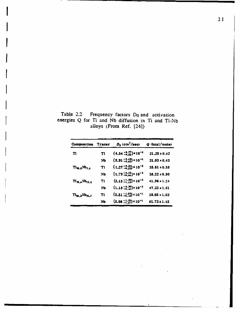
2.2 Frequency factors Do and activation energies Q for Tiand Nb diffusion in Ti and Ti-Nb alloys (FromRef. [24]) ............................................................................................. 2 1
2.3 The pre-exponential constants for diffusion of Aluminumin alpha Ti according to [40] and references therein ......... 30
2.4 The pre-exponential constants for diffusion of Aluminumin beta Ti according to [40] and references therein ...... 3 1
3.1 Ingot analysis of pure materials ................................................. 7 53.2 Alloy compositions ......................................................................... 773.3 Comparison of chemical analysis results for binaryU
alloy .' (Nb-4.5AI) ................... ............... 7 83.4 List of diffusion couples .............................. 854.1 Interstitial content of alloys (ppm) ..................................... 11 64.2 Temperature and concentration dependencies of the
interdiffusion coefficient in the system Nb-AlSsystem ................................ 15 1
4.3 Activation energy and frequency factor values forinterdiffusion in b.c.c. Nb-Al alloy a different AlScom position .................................................................................... 1 53
4.4 Intrinsic diffusivity of Al in (bcc) Nb .................................. 1554.5 Composition -dependent activation energy and
frequency factor values for intrinsic diffusion of Al ...... 1614.6 Solute diffusion in Nb-X system (From Ref. [77]) .......... 1 66I 4.7 Interdiffusivity data for the phases in the
Nb-Al system .............. ........................ 1685.1 Depth of penetration in ternary diffusion couples of
system (B.C.C.) Nb-Ti-Al .......................................................... 2 1 55.2 Kirkerdall shift measurements ................................................. 2295.3 Penetration ratios observed in the ternary couples
of this study ...................................................................................... 2 3 2
viii

Ip
9 LIST OF FIGURES
9 Figure Page
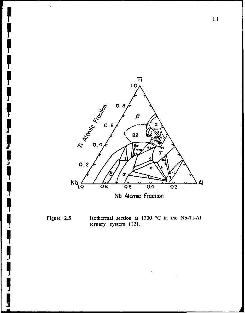
2 1 The Ti-Nb phase diagram [9] ..................................................... 62.2 The Al-Nb phase diagram [10] ................................................... 72.3 The Ti-Al phase diagram [ 11] ..................................................... 82.4 The Nb-Ti-Al Liquidus Projection [12] .................................. 1 02.5 Isothermal section at 1200 °C in the Nb-Ti-Al ternary
system [12] ............................................................................................ 1 12.6 Temperature dependence of the diffusion of Ti44
and V48 in titanium [18] ............................................................. 142.7 Computer fit of the experimental data for the diffusion
of Ti44 in titanium to the proposed by Kidson [19].(From [18]) ....................................................................................... 1 6
2.8 Measured diffusion coefficients of Ti (circles) and Nb(triangles) in different Ti-Nb alloys as a function oftemperature [24] ............................................................................ 1 9
2.9 Diffusion coefficients of Ti (circles) and Nb (triangles)as a function of composition for 3 different temperatures[24] ..................................................................................................... 2 0
2.10 Self-diffusion in b.c.c. metals. Plot of the self-diffusioncoefficient against the reduced reciprocal temperature[28] .......................................................................................................... 2 3
2.11 Concentration dependence of coefficient of mutual diffusionin Ti-Nb system: 1-1400°, 2- 1300', 3- 12000, 4- 11000, 5-1000 *C. From [30] ......................................................................... 24
2.12 Concentration dependence of activation energy and pre-exponential factor of mutual diffusion in the Ti-Nb system[30] ..................................................................................................... 2 5
2.13 Interdiffusion coefficients vs at% for the diffusion of Al in
ax-Ti. The present data obtained at 9000 and 635 'C arecompared with results published by 1) [38], and 2) [39].(From Ref. [36]) .............................................................................. 29
Six

Figure Page
2.14 The diffusivities of oxygen and Al in a-Ti. The numbersin the plot correspond to the series numbers in 'fable2.3 [401 .............................................................................................. 3 2
2.15 The diffusivities of 0, Al, and V in P-Ti. The numbers inthe plot correspond to the series numbers in Tables 2.4
[401 ........................................................................................................ 3 32.1 6 Diffusion coefficient as a function of reciprocal
temperature of unalloyed Nb, and apparent diffusioncoefficient for 2 Nb-Ti alloys [43] .......................................... 3 5
2.17 Parabolic rate constant vs Temperature for oxidationresistance materials [46] ............................................................. 3 8
2.18 Typical composition profile of an annealed diffusion couple.The Matano interface is positioned to make the hatched
areas on (cross hatched area), and the tangent valuesemployed to calculate the intertdiffusion coefficient at acomposition c= 0.2.co................................................................. 45
2.19 Atomic jumps in a b.c.c. crystal considered in the modelcalculation made by [59]. a) Type A: jumps to thenearest-neighbour position, b) Type B: jumps to the secondnearest-neighbor position, c) Type C: jumps to the thirdnearest-neighbour position ....................................................... 4 8
2.20 Potential barriers for the cited types of individual jumpsstarting at r= 0 and ending at r= 1. The maximum value ofeach curve corresponds to the migration energy for the
particular hopping event[59] ................................................... 49p 2.21 Migration energy for self-diffusion in dependence on thebinding energy of the crystal in comparison with theexperimental data refered therein. The line drawn presents
_ the calculated relation by [59] ................................................ 5 12.22 The Lattice Reference Frame .................................................... 5 552.23 Composition Paths in a teiliary system isotherm ............. 5 92.24 Evaluation of Matano integrals and slopes at a given
composition for evaluation of diffusion coefficients inI ternary system s ............................................................................ 62
2.25 a) The direct coefficient of diffusion for Cu, D 13 in units10-12 cm2/sec, at 725 'C. Filled circles indicate intersectionsof diffusion paths, and open squares indicate extreme pointsin the composition profile [65] ................................................. 64
x

Figure Page
2.25 Continue b) The direct coefficient of diffusion forAg D223 inunitslo- 12 cm2/sec, at 725 *C. Filled circles indicateintersections of diffusion paths, and open squares indicateextreme points in the composition profile [651 ................. 64
2.26 a) Model for a ternary diffusion couple with independentconcentration penetration tendencies; b) total concentrationcurve; c) computation of Kirkendall shift; d) prediction ofKirkendall shift; e) atom-fraction penetration profiles for
the unrelaxedlattice; and f) computed composition path[69] ..................................................................................................... 6 8
2.27 a) Model for a ternary diffusion couple with concentration
dependent penetration tendencies; b) total concentrationcurve; c) computation of Kirkendall shift; d) prediction ofKirkendall shift; e) atom-fraction penetration profiles forthe unrelaxed lattice; and f) computed composition path.Note the ondulation in component B (e) and thedisplacement of the crossover point on the path (f).[69] ..................................................................................................... 7 1
3.1 A flow chart showing the experimental procedure for
the preparation and analysis of the diffusion couples ....... 743.2 Furnace assembly used for all heat treatments
in this research ............................................................................... 803.3 Experimental set-up for hot-pressing bonding of diffusion
couples ............................................................................................... 8 44.1 Optical micrograph showing the dendritic microstructure in
a Nb-4.5AI alloy after arc-melted. Note the big columnargrains .................................................................................................. 9 2
4.2 A typical experimental composition profile for aluminumobtained by microprobe analysis showing themicrosegregation present in an arc-melted Nb-4.5AIspecim en ............................................................................................ 9 3
4.3 a) BSE micrograph, and b) a typical experimentalcomposition profile for Al obtained by microprobe analysisshowing microsegregation through a dendrite in an arc-melted Nb-4.5A1 specimen ........................................................ 94
4.4 BSE micrograph of the levitated and cooper-chilledquenched Nb-7.1AI alloy after homogenization at 1400°Cfor 2 hours and furnace cooling. Presence of particles Nb3A 1in the matrix (J phase) is observed ....................................... 96
xi

Figure Page
4.5 BSE micrograph showing the two-phase structureobtained in a Nb-4.5AI alloy after annealing at 14000Cfor 8.5 hrs ........................................................................................ 9 8
4.6 a) Secondary Electron micrograph, and b) EDX spectrumobtained from the matrix (P3 phase) of a Nb-4.5AI alloy after
annealing at 1400"C for 8.5 hours .......................................... 994.6 (Continued) c) EDX spectrum obtained from a precipitate
formed inside a grain of a Nb-4.5AI alloy after annealing at1400°C for 8.5 hours ................................................................... 1 00
4.7 a) Secondary Electron micrograph, and b) EDX spectrumobtained from a precipitate formed at the grain boundaryof a Nb-4.5AI alloy after annealing at 14000C for 8.5hours .................................................................................................. 1 0 1
4.8 Auger analysis of a precipitate located inside a grainof Nb-4.5AI alloy annealed at 14000C for 8.5 hours ......... 1 02
4.9 Standard Auger spectrum obtained from pure alumina[731 ......................................................................................................... 1 0 4
4.10 Auger spectrum obtained from the matrix (P3 phase)
of a Nb-4.5AI alloy after annealing at 1400 'C for8.5 hours ............................................................................................. 10 5
4.11 Optical micrographs showing the microstructure of a Nb-4.5A1 alloy after two different homogenization treatments:a) 1400 °C for 8.5 hours, b) 1400 'C for 6 hours ............ 1 06
4.12 A low magnification BSE micrograph of a Nb-4.5AI alloyafter being heat treated at 1400'C for 6 hours. Note howthe amount of alumina precipitation lessen from top
(sample surface) to bottom (sample middle section) ....... 1 074.13 BSE micrograph of a Nb-4.5AI sample as-homogenized
condition. Alumina presence in the P3-phase matrix is veryscarce ..................................................................................................... 1 0 9
4.14 a) Secondary Electron micrograph, and b) Al composition
profile of P3-phase matrix close to an alumina particle... 110.4.15 A low magnification BSE micrograph of a diffusion couple
with zirconia markers: a) Before diffusion treatment, andb) after diffusion treatment at 1400'C for 4 hours .......... 1 11
4.16 a) BSE micrograph of diffusion couple interface with Yttriamarkers before diffusion treatment, and b) the aluminumconcentration profile across the boundary ........................ 11 3
pi

Figure Page
4.17 Backscattered electron micrographs showing the resultantmicrostructures of a Nb/Nb-4.5Al diffusion couple afterdiffusion treatment. a) Near interface. b) Away frominterface .......................................................................................... 11 5
4.18 A typical experimental composition profile for aluminumobtained by microprobe analysis of a diffusion coupleNb/Nb-4.5AI after annealing at1450 'C for 4.5 hours. Notethe sudden drop in the Al composition profile in the Nb side
of the couple ................................................................................. 11 74.19 a) Secondary electron micrograph, and b) a typical
experimental composition profile for Al obtained bymicroprobe analysis of a Nb/Nb-4.5AI diffusion couple after
Sannealing at 1350 IC for 5.5 hours ...................................... 11 94.20 Schematic representation of the modified cubic spline
intervals employed for curve fitting ................................... 1 214.21 A typical composition profile for aluminum after incorrect
spline cubic fitting. Note the discontinuities along thecurve ..................................................................................................... 12 3
4.22 Fitting of experimental composition profiles by the splinecubic method for the Nb/Nb-4.5AI couple heat treated at1350 *C: a) Experimental carve,b) Fitted profile ........ 1 24
4.23 Fitting of experimental composition profiles by the splinecubic method for the Nb/Nb-4.5AI couple heat treated at1400 *C: a) Experimental curve, b) Fitted profile ....... 1 26
4.24 Fitting of experimental composition profiles by the splinecubic method for the Nb/Nb-4.5AI couple heat treated at1450 'C: a) Experimental curve, b) Fitted profile ....... 1 28
4.25 Fitting of experimental composition profiles by the splinecubic method for the Nb/Nb-4.5AI couples heat treated at1500 *C: a) Experimental curve, b) Fitted profile ....... 1 30
4.26 Fitting of experimental composition profiles by the splinecubic method for Nb/Nb-4.5AI couple heat treated at1550°C: a) Experimental curve, b) Fitted profile ............... 1 32
4.27 a) Typical calculated interdiffusion flux profiles forbinary diffusion couples Nh/Nb-4.5AI interdiffused at
1350 0C ................................................................................................. 13 54.28 b) Typical calculated interdiffusion flux profiles for
binary diffusion couples Nb/Nb-4.5AI interdiffused at1550 0 C ................................................................................................. 13 6
I xiii

I Figure Page
4.29 Typical calculated composition gradient and interdiffusioncoefficient profiles illustrating false peaks due to a baddesignation of parabolic regions during the fittingprocedure for binary diffusion couples Nb/Nb-4.5AIinterdiffused at 1550 'C. a) Derivative, b) Coefficient ofInterdiffusion ................................................................................ 1 38
S4.30 a) Composition gradient, and b) interdiffusion coefficientprofiles for Nb/Nb-4.5AI diffusion couple heat treated at1350 oC ................................................................................................. 14 1
4.31 a) Composition gradient, and b) interdiffusion coefficientprofiles for Nb/Nb-4.5AI diffusion couple heat treated at1400 OC ................................................................................................. 14 3
4.32 a) Composition gradient, and b) interdiffusion coefficientprofiles for Nb/Nb-4.5AI diffusion couple heat treated at1450 0 C ................................................................................................. 14 5
4.33 a) Composition gradient, and b) interdiffusion coefficient
profiles for Nb/Nb-4.5AI diffusion couple heat treated at1500 0 C ................................................................................................. 14 7
4.34 a) Composition gradient, and b) interdiffusion coefficientprofiles for Nb/Nb-4.5AI diffusion couple heat treated atI 1550 °C ................................................................................................. 14 9
4.35 Dependency of the interdiffusion coefficient on the Alcomposition at several temperatures .................................. 1 52
4.36 The temperature dependency of the intrinsic diffusion
coefficient of Al in Nb at the aluminum concentration of3.0 at% .................................................................................................. 15 6
4.37 The temperature dependency of the intrinsic diffusion
coefficient of Al in Nb at the aluminum concentration of2.5 at% .................................................................................................. 1 5 7
4.38 The temperature dependency of the intrinsic diffusioncoefficient of Al in Nb at the aluminum concentration of2.0 at% ................................................................................................. 1 5 8
4.39 The temperature dependency of the intrinsic diffusioncoefficient of Al in Nb at the aluminum concentration of1.5 at% .................................................................................................. 1 5 9
4.40 The temperature dependency of the intrinsic diffusioncoefficient of Al in Nb at the aluminum concentration of1.0 at% .................................................................................................. 1 6 0
4.41 Comparison between this work and Ref. [6] for thetemperature dependence of the diffusion coefficientof A l in N b ........................................................................................... 16 3
xiv

Figure Page
5.1 Schematic representation of the ternary diffusion couplesemployed in this research ........................................................ 1 7 1
5.2 Micrographs showing the duplex structure (a+J3) of the as-received Ti: a) Optical micrograph, as-etched condition; b)B SE im age ............................................................................................ 17 4
5.3 BSE micrograph of 131 alloy (Nb-42.5Ti-15AI) afterhomogenization at 1400 'C for 6 hours .............................. 1 75
5.4 Optical micrograph of the bonded interface in diffusioncouple #12 (131/Ti) after bonding at 700 *C for 2 hoursshowing the duplex structure a+13 of the Ti side of thecouple ............................................................................................... 1 7 6
5.5 a) BSE micrograph of interface in diffusion couple#12 (131/Ti) before diffusion treatment; b) the three
composition profiles across the boundary ......................... 1 77S5.6 Optical micrograph of the Ti side next to the bondedinterface in diffusion couple #12 (131/Ti) after diffusiontreatment at 1200 'C for 6 hours. Note the duplex (a+13)zone with the acicular morphology next to theinterface ......................................................................................... 1 79
5.7 Optical micrograph showing precipitation of a phase atthe interface and grain boundaries of the ternary 13I(Nb-42.5Ti-15AI) side of the couple after bonding at900 'C for 2 hours ........................................................................... 180
5.8 BSE micrographs showing precipitation of a phase in theternary side of the couples along the interface:a) diffusion couple #9 (131/133); and b) diffusion couple#11 (132/130) ........................................................................................ 18 1
5.9 BSE micrograph of bonded interface in diffusion couple#10 (021p3) after bonding at 900 'C for 2 hours showingthe presence of second phase (a)on both sides of theinterface ......................................................................................... 1 82
5.10 BSE micrograph of the interface in diffusion couple #6(131/Nb) after diffusion treatment at 1400 'C for 6 hours.Microprobe analysis contamination over the precipitation-free structure is detailed .......................................................... 1 83
xv

Figure Page
5.11 BSE micrograph of the 132 side away of the interface ofdiffusion couple #10 (132/133) after diffusion treatmentat 1200 °C for 6 hours, and subsequent treatment at920 0C for 2 hours. Reprecipitation of the second phaseis observed .......................................................................................... 1 8 5
5.12 Penetration curves of the 3 components in the couple#6 (131/Nb), heat treated at 1400 °C for 6 hours ............ 1 86
5.13 Penetration curves of the 3 components in the couple#7 (031/133), heat treated at 1400 °C for 6 hours ................. 1 87
5.14 Penetration curves of the 3 components in the couple
#8 (131/Nb) heat treated at 1200 °C for 6 hours ................. 1 88U 5.15 Penetration curves of the 3 components in the couple#9 (131/133), heat treated at 1200 'C for 6 hours ................. 1 89
5.16 Penetration curves of the 3 components in the couple#10 (132/133), heat treated at 1200 *C for 6 hours .............. 1 90
5.17 Penetration curves of the 3 components in the couple#11 (132/130), heat treated at 1200 'C for 6 hours ............... 1 9 1
5.18 Penetration curves of the 3 components in the couple#12 (131i/Ti), heat treated at 1200 °C for 6 hours ............... 1 92
5.19 Penetration curves of Al in three different diffusioncouples heat treated at 1200 °C for 6 hours ..................... 1 94
5.20 Penetration curves of Nb in three different diffusioncouples heat treated at 1200 *C for 6 hours .................... 1 95
5.21 Penetration curves of Ti in three different diffusionScouples heat treated at 1200 °C for 6 hours ..................... 1 965.22 Composition profiles of Al in diffusion couples #9 and #10
after heat treatment at 1200 'C for 6 hours ............ 975.23 Composition profiles of Nb in diffusion couples #9 and #10
after heat treatment at 1200 °C for 6 hours .................... 1 985.24 Composition profiles of Ti in diffusion couples #9 and #10
after heat treatment at 1200 °C for 6 hours .................... 1 99
5.25 Composition profiles of the 3 components at constant Alconcentration (couple #9 131/133)) after heat treatment at1200 *C for 6 hours ........................................................................ 200
5.26 Comparison of penetration depth of Al in couples involvingalloy 132 (#10 (133/132) and #11 (130/132)) ...................................... 201
5.27 Comparison of penetration depth of Nb in couples involvingalloy 132 (#10 (133/132) and #11 (130/132)) ..................................... 202
xvi

Figure Page
5.28 Compariscn of penetration depth of Ti in couples involvingalloy 132 (#10 (133/132) and #11 (130/132)) ..................................... 203
5.29 Critical point observed in the Al composition profile afterdiffusion treatment of couple #11(130/132) at 1200 'C forh2hours ..................................................................................................... 2 0 5
5.30 Critical point observed in the Nb composition profile afterdiffusion treatment of couples #7 (130/132), #9 (133/131) and#10 (133/132) at 1200 'C for 6 hours .......................................... 206
5.31 Critical point observed in the Ti composition profile afterdiffusion treatment of couple #9 133/131 at 1200 'C for 6
hours ..................................................................................................... 2 0 75.32 Composition profile for Al after interdiffusion treatment at
1200 *C (#8) and 1400 *C (#6) for 6 hours ......................... 2095.33 Composition profile for Nb after interdiffusion treatment at
1200 *C (#8) and 1400 *C (#6) for 6 hours ....................... 2105.34 Composition profile for Ti after interdiffusion treatment at
1200 'C (#8) and 1400 *C (#6) for 6 hours ...................... 2 115.35 Composition profile for Al after interdiffusion treatment at
1200 *C (#7) and 1400 *C (#9) for 6 hours .......................... 2125.36 Composition profile for Ti after interdiffusion treatment at
1200 *C (#7) and 1400 'C (#9) for 6 hours ..................... 2 1 35.37 Composition profile for Ti after interdiffusion treatment at
1200 *C (#7) and 1400 TC (#9) for 6 hours .......................... 2145.38 Composition path for diffusion couple #8 (131/Nb), and
schematic representation of the crossover displacement.A Middle point composition
O M atano plane composition .................................................... 2195.39 Composition path for diffusion couple #6 (131/Nb). and
schematic representation of the crossover displacement.A Middle point composition.SM atano plane composition .................................................... 220
5.40 Composition path for diffusion couple #11(130/132).andschematic representation of the crossover displacement.A Middle point composition0 M atano plane composition .................................................... 222
SI xvii
pAbstract of Thesis Presented to the Graduate School of
the University of Florida in Partial Fulfillment of3 the Requirements for the Degree of Master of Science.
EVALUATION OF THE DIFFUSIVITY OF ALUMINUM INNIOBIUM BASED ALLOYS
BYp J. G. LUIS RUIZ APARICIO
DECEMBER 1990
Chairperson: Dr. Fereshteh Ebrahimi
Major Department: Materials Science and Engineering
F• Niobium alloys with improved resistance to oxidation are
needed for use as structural alloys. The feasibility of forming
protective alumina scales in Nb-AI-X alloys by the selective oxidation
of aluminum has been demonstrated and also has been shown that a
low aluminum diffusivity is the major factor limiting the selective
5• oxidation of aluminum. Additions of certain elements such as
titanium are thought to have a beneficial action on accelerating this
.1 diffusivity but information on the effect of alloying additions is
limited.
In this thesis, diffusion studies in the binary Nb-Al system by
ji the Matano-Boltzmann method, and diffusion analyses in the ternary
Nb-Al-Ti system thrcugh concepts such as Kirkendall shift, crossover
I displacements, penetration tendencies and composition paths, were
conducted to evaluate the diffusiv'v.y of Al and the effect of Ti on Nb-
based alloys.
3 Nb-Al, Nb-Ti, Nb-Al-Ti (b.c.c.) solid solutions were prepared by
arc-melting and were homogenized in a high vacuum furnace before
the fabrication of diffusion couples. Bonding of the diffusion couples
i xix

p was obtained by hot pressing in a temperature range of 7000 to 1000
0C for two hours. A fine dispersion of yttiria chopped fibers was used
as markers. The diffusion treatment temperatures were varied from
13500 to 1550 *C and 1200 0C to 1400 °C for the binary and ternaryF studies respectively. Microprobe analysis was employed for the
evaluation of composition profiles in all the diffusion couples.
Tne interdiffusion coefficient for the 0 solid solution of Nb-Al
system varied linearly with Al concentration in the range of 1-3 at%I: and it followed a linear Arrhenius behavior as a function of
temperature in the range of 1350 *C-1550'C. The average activation
energy for diffusivity of Al in Nb was calculated to be 78.4 Kcal/mole
with a frequency factor of 4.5 x 10⁻² cm2 /sec. These values are
smaller than those reported in the literature for a higher
I• temperature range. This discrepancy is attributed to the differences
in the evaluation method and the temperature range. The influencep of divacancy mechanism, which is known to operate at higher5 temperatures in Nb, may account for the higher diffusion rate and
activation energy.P• The composition path and penetration tendencies in the Nb-Ti-
Al system suggest that Ti is the fastest element in the J0 solid
solution. Qualitatively the penetration tendencies correlate with the
melting point of the alloys. The results of Kirkendall shift
measurement were found to be in agreement with the calculated
crossover displacement. The results obtained in this study suggest
that the addition of Ti to the binary alloy increases the general
diffusivity of the system.
Ix

CHAPTER 1INTRODUCTION
During the last decade, the necessity of both higher
performance requirements and new applications for spacecrafts has
renewed the interest in the development of advanced aerospace
materials. The aerospace industry has set the reduction of aircraft5 weight, extension of flying ranges, increment of payloads and
shortening of take-off requirements among its permanent objectives.
The accomplishment of these goals demands the development of
materials with improved physical and mechanical properties such as
strength to density ratio, fatigue resistance, high temperature
rupture strength, creep resistance, high temperature corrosion
resistance and fracture toughness. Currently, it is thought thatI. aircraft engines work at half of their potential horsepower due to
limitations such as strength and melting point of the existing high-
temperature Ni-based superalloys, which are the major structural
material used in military aircraft turbine engines. State-of-the-art
superalloys are limited in temperature capability to 1100 0 C.
However, there is an immediate need for a metallic material capable
of withstanding temperatures up to 1400 °C.
I Because of their special properties at high temperature,
refractory alloys were considered in the development of aerospace
materials in the early '60's, when aircraft and aerospace. nuclearII.I

I 2
5 propulsion were developed. Among these refractory metals, the5 lower density niobium alloys were investigated for turbine
applications. Their long-term, high -temperature strength, ductility,
p and creep resistance are well retained at high temperatures,
comparable to those obtained in nickel-base superalloys, but their
poor oxidation resistance in environments rich in atmospheric gas
species [1, 21 and the arrival of superalloys properly cooled halted
their development [3]. At present, niobium alloys are used in non-
critical sections of aircraft engines, like exhaust nozzle components,
where their high melting temperature are needed.I A recent approach to solving the problem of poor oxidation of
many high temperature structural materials is the addition of
aluminum as an alloying element. Alumina A1203 is a stable oxide
that usually shows a good adherence to the metallic alloys. There are
two main problems associated with the oxidation behavior of theU aluminum containing high temperatures alloys. In the case of alloys3 such as Fe-Cr-Al, the fast diffusion of cations through the alumina
scale leads to the occurrence of the oxidation process at gas/oxide
interface and consequently voids are formed at oxide/metal
i nterface, which results in oxide spallation and poor adherence of theI oxide to the alloy. In the case of Nb alloys it has been suggested [4]3 that the slow diffusivity of aluminum prevents the continuous
formation of alumina and transition oxides are rapidly formed and3 hence undesirable high oxidation rates are achieved. Oxidation
studies on Nb-Al alloys [5] have indicated that a minimum aluminum
content of 50 at% is required to obtain a continuous alumina scale.

3
The addition of alloying elements such as Ti, Mo and V has been
shown to reduce the oxidation rate of Nb alloys.
Although the poor oxidation resistance of the Al containing Nb
alloys has been related to the low diffusivity of Al, there have been
very limited studies [6) in which the diffusivity of Al in Nb has been
measured indirectly. The purpose of this research was to evaluate
the diffusivity of aluminum in binary Nb-Al and ternary Nb-Al-Ti
solid solution alloys. The experimental approach used in this study is
based on the diffusion couple technique [7] with post-diffusion
treatment evaluation of composition profiles by electron microprobe
analysis (EPMA). Optical and scanning electron microscopy (SEM)
methods were employed for the evaluation of the microstructure.
The alloys were prepared by arc-melting of high purity metals. The
diffusivity measurements were conducted in the temperature range
of 1350 °C to 1550 °C for the binary case and 1200 °C to 1400 *C for
the ternary one.
The first part of this thesis approaches briefly the theory of
diffusion from both a phenomenological and an atomistic point of
view. In addition, a mathematical analysis of the theory is presented
as it provides the basis for the Fortran-77 source code [8] used for
the evaluation of the coefficient of diffusion of Al in the binary
system. The basis for the experimental techniques employed through
this work, as well as a review of the previous work done in the
binary Nb-AI system and the ternary Nb-Al-Ti system are also
presented in this chapter. Chapter 3 simply describes the materials
used and the experimental procedures followed throughout this
research. The results for the binary Nb-Al system and for the

* 4
ternary Nb-Al-Ti system are presented and discussed in Chapters 4
and 5, respectively. Results in Chapter 4 include a discussion about
the experimental difficulties found during the preparation of the
binary alloy Nb-Al used in the binary couples. The discussion of the
ternary diffusion results in Chapter 5 is based on a phenomenological
approach of basic concepts such as composition paths, Kirkendall
-- displacements and penetration tendencies. A summary of results for
binary and ternary diffusion is given at the end of the respective
3 chapters, with the final conclusions of this research presented in
-- Chapter 6.
I
U
I

IIII
CHAPTER 2LITERATURE REVIEW
This chapter is divided into three sections. First the literature
concerning the Nb-Ti-AI system is reviewed. The subjects prevalent
to this section include phase stability, diffusivity and oxidation in
I ternary and the constitutive binary systems. The second part of this
review concentrates on the mathematical formalism and mechanisms
I of diffusion in binary and ternary systems consisting of single phase
crystalline materials.
2.1 Nb-Ti-Al systemI2.1.1 Phase diagram
This section is devoted to establish the limits of both
tempe ature and composition for the b.c.c. P3 phase in the Nb-Al-Ti
I ternary phase diagram.
The binary diagrams composing this ternary system are
presented in Figures 2.1-2.3. The Nb-Ti system, Figure 2.1, features
an isomorphous-type, complete solubility of both components in a
b.c.c. phase at temperatures above 882 0C at the Ti side [9]. This
phase field extends to room temperature as Nb content increases.
5

1 6
Ij Weight Pleraent Nootasum
II
TI Atomic Percent Niobium Nk
5Figure 2.1 The Ti-Nb phase diagram [9].

40 wog~fat Percent Niobium0 00 N30 4* so so 79 g
Ij a-a,- L
'4"4"
0.4
SA: Atmi julen N-bmM
Figue 22 Th AINb pasediagam 10]

:I
IWOJ Reotihi P'•re.ent A|:s~nnlanm
toI 2S -30 4, sf 41 ,O 7g • .
l]4-
*U b (PTI)
"Am TIAInum .
E Ti3AI :
-TA1IaI
aTIA1.3 (AI)-
O 30 0 36 40 so 7O 40 is lTi Atomic Percent Aluminum Al
Fi2ure 2.3 The Ti-Al phase diagram [11].IIIIl!I__
9
The other phase present is the h.c.p. a-Ti phase, which is stable at
high Ti contents and temperatures below 882 "C.
Nb-Al and Ti-Al systems exhibit intermetallic compound
formation, namely: (12-Ti 3Al (DO19), y-TiAl (LI0), and ri-TiAl 3 (D022) in
the Ti-Al system, and 8-Nb 3Al (A15), a-Nb 2 Al (D8B), and -I-NbAl3
(D022) in the Nb-Al system, in addition to the terminal solid
solutions. The solubility of Al in Nb at room temperature is not very
well established. The phase diagram [10] suggests a solubility limit of
!1! 7.5 at%. Maximum solubility of Al in b.c.c. Nb is 23 at% which is
reached at 1960 'C. The 03 phase in the Ti-Al [11] phase diagram is
stable only at elevated temperatures. The solubility of Al in JP-Ti
I increases with temperature, reaching a 48.5 at% maximum solubility
at 1475 OC.
SThe ternary Nb-Al-Ti system has been the subject of several
investigations during the last decade as a result of the recent activity
Ii on development of alloys for high temperature applications. It is a
rather complicated system featuring several transition equilibria.
Perepezko et. al. [12] and Kaltenbach et. al. [13] recently have
* performed a systematic evaluation of this system including mappings
of liquidus projections and determination of isothermal sections of
I the system at 1200 °C. Both studies show excellent agreement with
each other and studies made by Benderzky et al. [14] and Jewet et.
al. [15]. Examples of liquidus projections and the isothermal section
at 1200 *C are given in Figures 2.4 and 2.5. The liquidus surface
features several four-phase equilibria (I-IV) with the subscripts 1,
l 2,... indicating the temperature sequence (1 higher than 2). In
i accordance with [12], the binary invariant reactions are represented
SI

p 10
1.0 tool"
I I.0.8
S0.6
0 ,. ,1 \
!0.4-4 ~ p 44 g 370
41a3:01
N- r1. . , ft I6 to 0.4
Nb Atmi Fraction
INbAoi!Fato
10TiII
.•0
0.
Nb . .. Al1.0 0.8 0.6 0.4 02
SNb Atomic FractionIFigure 2.5 Isothermal section at 1200 °C in the Nb-Ti-Al
ternary system [121.'I,II

1 12
as pi (peritectic) and ei (eutectic). There is only one saddle point in
the system which is indicated by an open circle in Figure 2.4. The
arrows inscribed upon the lines show the directions of the slopes for
the univariant equilibria (liquidus valleys) toward lower
temperatures.
It is observed that the liquidus valleys decrease in
temperature from the high temperature peritectic points in the Nb-
Al side swinging clockwise towards the Al corner of the triangle. The
13-phase surface exhibits the highest melting points and it covers a
big range of the total area of the liquidus projection surface. The
large solubility of Al in 03 phase decreases with temperature. This can9 be observed by contrasting the extension of the 13-phase field of the
liquidus projections with their respective isotherm at 1200 *C. In
accordance with these projections, the solubility limit for Al in the
b.c.c. solid solution depends on both the temperature and the Nb (or
I Ti) content. As the temperature is raised and the Ti content
increased, Al becomes more soluble.
2.1.2 Diffusivity
I In general, 'normal' diffusion in metals is characterized by the
following properties 1,61:
1) Do and Q are temperature independent over a wide range of
temperatures,
2) DO lies in a range of 0.05 to 5 cm2/sec,
3) Q (cal/mole) is approximately equal to 34.Tm (melting
temperature, K),
SI

F 13
4) The diffusion value for substitutional impurities is within an
order of magnitude of the self-diffusion rate of the host atoms.
In accordance with diffusivity investigations, there are a number of
b.c.c. metals which show anomalous diffusion behaviors. They do not
present "normal" diffusion. For these metals the Arrhenius plot
presents a curvature that is more pronounced than that seen in f.c.c.P metals, for which is a result of divacancies contributions [17]. As
mentioned earlier, the Ti-Nb system exhibits a complete solubility in
b.c.c. phase at elevated temperatures. Ti, among others, is one of
these b.c.c. metals with anomalous behavior [18]. Murdock et. al. [18]
found that In D vs l/T plots for diffusion of Ti44 in Ti were fitted best
by a line of continuous curvature (Figure 2.6), which indicated an
increase in Q and Do with the temperature. They proposed the model
that Kidson [19] used for the diffusivity of Zr (b.c.c.) to explain their
results. In accordance with this model, there are two competing
volume diffusion mechanisms operating in the two temperature
regions: intrinsic and extrinsic. He [19] attributed the low-
temperature 'extrinsic' region to the presence of a temperature-
independent concentration of vacancies due to the presence of
impurities, like oxygen atoms, which cause the concentration of this
type of vacancies to be much greater than the concentration of
'intrinsic' or thermal vacancies at low temperature. The total curve
can be obtained by the sum of 2 exponential terms representing each
of these contribution. The resulting equation obtained by Murdock et.
al. [20] for the Ti case is:
DTi 44= 3.58xiO-4 exp(-31,200IRT) +
1.09 exp(-60,000/RT) cm2 /sec .......... (2.1)
I

14
IITEMPERATURE VC)
woo 15W AWO 1300 QOO 1100 to00 900
U*2 _ _ _
I v lo nw ---
- 2
16 *
0.5 0.6 00.9
l;Figure 2.6 Temperature dependence of the
II diffusion of Ti44 and V48 in titanium[181.
II
I .. I"••

I '!U
X _ _
0 . 5 0 6 0 ? 0.6 0..I!
Figure 2.7 Computer fit of the experimentaldata for the diffusion of Ti4 4 intitanium to the proposed by Kidson[191. (From [181).
I.1I

p 17
Cu
0 ca a 00en 00
Z; uC.)~Fl UU r
-xFC% 00
'IC.)

Pi 18
p the Arrhenius plot which they assumed was caused by a divacancy
effect at high temperatures and was fitted by the expression:
D= (3.7+0.3) exp(-4.54 eV/kT) +
(8±3) x 10-3 exp(-3.62 eV/kT) cm 2/s .......... (2.2)
Pontau and Lazarous [24] experimentally evaluated the diffusivity ofI Ti and Nb in b.c.c. Ti-Nb alloys at different concentrations, which9 were chosen to avoid the a/P3 transition and to obtain the metastable
co phase [25]. This co phase as discussed earlier is thought to enhance
diffusion in other b.c.c. materials like Ti and Zr [20, 261. They [24]
determined simultaneously the diffusion coefficients for Ti and NbI radioactive tracers over the temperature range of 950*-1511 'C
using lathe-sectioning techniques. Their results are presented in
Figures 2.8 and 2.9 and Table 2.2. They found no evidence of
anomalous behavior in the diffusivity behavior, except for low values
of DO and Q compared to those reported by [27]. Their Arrhenius
plots were moderately curved, but due to lack of enough points an
accurate two exponential fit to their data could not be performed.
They did not found any evidence that supported the enhancement of
diffusion at low temperatures by the presence of wo-phase nor via
dislocations, and concluded that an operating normal relaxed
vacancy-divacancy mechanism was consistent with their results.
Newmann and Tolle [28] recently analyzed the published data
in self-diffusion of b.c.c. metals by assuming a two-defect model and
various one-defect models. They found that Nb self-diffusion data
"could be fitted accurately by the 2-exponential model proposed by
Eizinger et. al. [23]. They pointed out that oxygen contents up to 800
p.p.m. have no influence on the diffusion coefficient. In accordance
III ~ n annum ~ m • - - - -. .

19
T"1;OM4 0.4j5.6
,N5 .7 ____ 5_ ____ 7
Figure 2.8 Measured diffusion coefficients of Ti (circles)
and Nb (triangles.) in different Ti-Nb alloys as a
function of temperature [24].II
I ,0 56 f 6468 . 768

20
IiIdr
I _ _ _ _ _ _ _ _ _ _ _ _ _ _ _ _ _ _ _ _ _ _ _ _ _ _ _ _ _ _ _ _
I a 1511"C
I
I IA
- ( I I , I Ii010
to 0% 0 30%I Atom % l7. wff
Figure 2.9 Diffusion coefficients of Ti (circles) and Nb(triangles) as a function of composition for 3different temperatures [241.
I21
III
Table 2.2 Frequency factors Do and activationenergies Q for Ti and Nb diffusion in Ti and Ti-Nb
alloys (From Ref. [241)
Composition Tracer D9 (cm-/sec/ Q fkcal/mole)
TI Tt (4.34 ::-)x 10"' 31.30 * 0.43
-(2.9 x 10⁻⁴ 31.03 a 0.43
TI,.ANb. TI (t.• •jIJ • 10" 35.61 * 0.58
Nb (1.79 : 10-, 38.22 zO.sO
Tls.49b,. TI (3.15 :•;:)x 10-' 41.96 * 1.24
Nb (.S:::;")x1o" 47.33 1.61
TI.3,4b 1.? TI (2.351.":!) x10 59.02 a 1.03
Nb (2.98 :l:,",)x 101 61.73* 1.45

22
with their analysis, ".c. metals can be divided in three groups:
Group IVb (Ti, Zr, Hf) where the metals show an abnormally high
diffusivity at low temperatures, Group V and VI (refractory metals)
which show a more or less normal behavior, and Group I (alkaline
metals) which fall in between the previous two. This classification is
better observed in the normalized plot in Figure 2.10. They
concluded that one-defect mechanism is improbable for both
refractory and alkaline b.c.c. metals, but they could not discuss either
the nature of the diffusion mechanisms that operate at high
temperature.
Hu An et. al. [29] measured the interdiffusivity of the Nb-Ti
system at low temperatures (300 *-350 'C) using X-ray diffraction
techniques in compositionally modulated structures with an initial
content of 50 at% Ti and 50 at% Nb. They determined a value lower
than 10-20 cm 2/sec for the interdiffusion of the system, which is in
agreement with the diffusivity results obtained at high temperature
by Ugaste and Zaykin [30] using tracer technique. Ugaste and Zaykin
[301 also investigated the concentration dependence of the
interdiffusion coefficient in this system. Figure 2.11 shows a
comparison of their results with those from other authors which
prove to be completely inconsistent. Figure 2.12 also gives the
concentration dependence of the activation energy Q and the pre-
exponential factor Do. Despite the inconsistency in concentration
dependence of D values, the Q values seem to he consistent with the
values given in Table 2.2. In general, D increases strongly with the Ti
concentration, which is consistent with the concentration dependence
of the solidus temperature. Consistently, the activation energy

1 23
I1 -6-
p O_7-10-41_
0U -Z
TraiTio'To
5 10-15
Figure 2.10 Self-diffusion in b.c.c. metals. Plot of theself-diffusion coefficient against thereduced reciprocal temperature [281.
I!

p24
loIU
10-IwNt.% 77"I
Figure 2.11 Concentration dependence of coefficientof mutual diffusion in Ti-Nb system:1-1400, 2- 13000, 3- 12000, 4- 11000,5- 1000 *C. From [301.
,II

P 25
I
50
0
60 o , 0
NDA% 7t
Figure 2.12 Concentration dependence of activationenergy and pre-exponential factor ofmutual diffusion in the Ti-Nb system[30].
I

rI 26
I increases with the Nb content.
The only information available on the diffusivity of Al in Nb is
the back-calculated diffusivity from the evaporation rates of
aluminum from dilute Nb-Al alloys conducted by Nikolaev and
Bodrov [6]. In accordance with their experiments, the aluminum
diffusivity follows an Arrhenius behavior that can be expressed as:
DAI= 450+/-10 exp[-(102730 +/- 7 000)/RT) cm2/sec ...... (2.3)
They evaluated *he thermodynamic and kinetic characteristics of the
evaporation of aluminum present in niobium as an impurity (10-2-
10-3 at%) by atomic absorption spectroscopy in an argon atmosphere.
Their proposed method to measure the diffusivity of impurities in9 the solid phase is based on measuring the rate of decay of the atomic
absorption by plotting the kinetic curves for the evaporation process.
9 They found that at a given temperature the concentration of
aluminum vapor over the sample stays close to the equilibrium value
for a short period of time (30 seconds), followed by a steep fall of the
vapor pressure curve due to a depletion of aluminum from the
surface of the sample. After measuring the absorption of aluminum
9 vapors from pure aluminum and alloys containing a known amount
of it, they calculated the Al activity coefficient and its temperature
dependence. From these experiments they were able to determine
I the kinetics of the evaporation process, that is, the motion of the
atoms in the solid phase. During the first part of the process the
3 transport of the aluminum atoms from the surface of the sample is
achieved by evaporation. The subsequent decay of the absorption
I curve denoted a rate limitation on the availability of aluminum
atoms caused by the diffusion of the aluminum in the niobium. They
!

P 27
implied that the diffusion step of the evaporation process obeyed the
expression 131):
Ns(t)/Nos = exp [y2 ] erfc (y) (2.4)
where NS(t) and Nos are the aluminum concentrations at the surface
of the sample at the time of the measurement and at the beginning
of the experiment respectively, and
y2= p32 tDs (2.5)
where DS is the diffusion coefficient to be calculated and 03 is an
experimental constant. In accordance with their research this method
offers speed of operation, continuous observation of the diffusion
process, and application to the solid state diffusion of alloy3 components at the impurity concentration level (<10-2 at.%).
However, the method is not direct and is based on many
assumptions.
Raissanen et. al. [32] investigated the diffusivity of Al in
polycrystalline ion-implanted a-Ti in the temperature range of 600
'C to 950 *C using ion-beam techniques. They found the following
expression for the coefficient of diffusion:
D (cm 2/sec) = 7.4x10- 7 exp[-1.62 (eV)/kT] .......... (2.6)
Pokoev et. al. [331 also investigated the Al diffusivity in a-Ti using x-
ray diffraction techniques at 700-850 °C in a vapor deposited Al
layer on Ti foil. They found that the temperature dependence of the
diffusion coefficient is given by the following equation:
D (cm 2/sec) = 9.7x10⁻⁵exp [27,500 (cal/mole)/RT] (2.7)
Chaplanov et. al. [34] conducted annealings on Ti-Al films at 200-500
""C temperature range. Below 300 DC interdiffusion occurred with
subsequent formation of Ti-Al solid solutions. However, above this
I

28
temperature intermetallic phases such as TiAI3 , TiAl were formed.
The formation of a TiA13 has been reported elsewhere [35-37]. Zhao
et. al. [35] studied the reaction kinetics of Ti films on Al substrate at
450-550 'C, and found that the formation of a TiAI3 layer always
occurs at the Ti/AI interface. Rao and Houska [36] studied the inverse
case, i. e. Al film-Ti substrate, and found the same TiAI3 layer
formed. However, when the film was initially heated up to 900 "C,
there was a release of Al into a -Ti in the first stages, but longer
annealing times eventually led to the decomposition of the TiAI3
layer with a substantial release of Al into the substrate. According
with their results, the variation of the coefficient of diffusion with
composition was less than one order of magnitude when the
composition changed from 0 to 20 at% (Figure 2.13) [38, 39]. Because
p of the limited solubility, they could not calculate accurately the
coefficient of diffusion for the TiA13 phase, but it was estimated that
it tended to be one order of magnitude smaller than the diffusion in
the ot-Ti (Al) phase at 900 *C.
Liu and Welch [40] made a survey of the diffusion data
for aluminum in both a- and 13-Ti. Tables 2.3 and 2.4 show the pre-
exponential and activation energy of aluminum diffusion in a- and 13-
Ti, respectively, and Figures 2.14 and 2.15 present the Arrhenius
plots coefficient of diffusion. The Al diffusion data in a-Ti show poor
agreement as they are scattered. As to the diffusivity data for 13-Ti
phase, again the differences in the reported values for Al are
considerable, and no clear explanation is offered about it.
The diffusion of interstitial elements in Nb-Ti and Ti-Al alloys
has been extensively studied. Vasileva et. al. [41], for example,

p 29
p0 (1) 900-C
I
'a
*1
10' PRESENT 6350C
(2)6356C
0.00 10 20
% AL
Figure 2.13 Interdiffusion coefficients vs at% for thediffusion of Al in oc-Ti. The present dataobtained at 9000 and 635 0 C arecompared with results published by 1)[38], and 2) [391. (From Ref. [36]).
I

30
Cuu
- L.2
.I~i <~~P P
-U,.
-' T oo
ux 2 x xX
U~--a.--D
CV.1
CuLE~

a W%
I- 0
-: E * x xx
CCU o ~Eas-

P 32
Temoerature (°C)
I I _ _
P -
i. i i iji-t,
- I I *' i 1
S-m" -----.----.--- _ ,,_
11 ( -1
numer in Tal 2 "+: " .I3N [401.
p + + I t, IM I +
24 I IFIi __ _ __0.5 0.1/ 0.3 ~ 1. I i .S I.7P l.g
SFigure 2.14 The diffusivities of oxygen and Al in a-Ti. The
numbers in the plot correspond to the series
numbers in Table 2.3 [40].
I
I

I 33
Temperature (OC)Aw1100 Soo...7TO 60
4 IAit I
,, ••,\VI ____- __
v 1L-12 ,%
p '1 L i1E4
- i - JI7t -
0.5 0.7 0.9 1.1 1.3 1.5
1l/T (K-") X10-8
P Figure 2.15 The diffusivities of 0, Al, and V in P-Ti.
The numbers in the plot correspond tothe series numbers in Tables 2.4 [40].
II
34
determined the activation energies for N diffusion at 600-800 'C in
Nb (21.2 kcal/mole), and Nb-10 at%Ti (26-26.2 kcal/mole). Lauf [421
studied the effect of additions of substitutional solutes to Nb in the
oxygen diffusivity. He found that additions up to 5 % of Ti resulted in
a decrease of the 0 diffusivity in as much as one order of magnitude.
It was suggested that this was caused by trapping of oxygen by
substitutional solute atoms, with a substitutional/oxygen binding
energy of 0.6-0.8 eV for the Ti case.
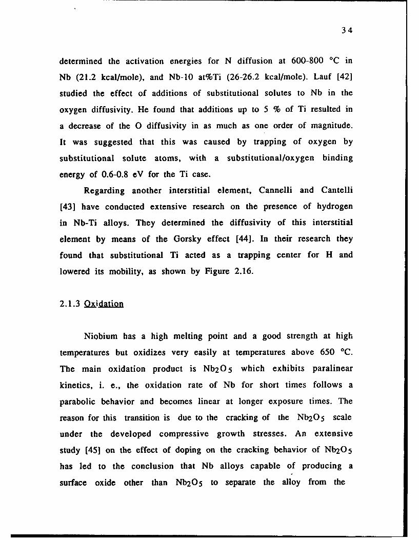
Regarding another interstitial element, Cannelli and Cantelli
[431 have conducted extensive research on the presence of hydrogen
in Nb-Ti alloys. They determined the diffusivity of this interstitial
element by means of the Gorsky effect [44]. In their research they
found that substitutional Ti acted as a trapping center for H and
lowered its mobility, as shown by Figure 2.16.
2.1.3 Oxidation
Niobium has a high melting point and a good strength at high
temperatures but oxidizes very easily at temperatures above 650 0C.
The main oxidation product is Nb205 which exhibits paralinear
kinetics, i. e., the oxidation rate of Nb for short times follows a
parabolic behavior and becomes linear at longer exposure times. The
reason for this transition is due to the cracking of the Nb205 scale
under the developed compressive growth stresses. An extensive
study [45] on the effect of doping on the cracking behavior of Nb20 5
has led to the conclusion that Nb alloys capable of producing a
surface oxide other than Nb205 to separate the alloy from the

35
-s 500400 300 T 2K)
llV Nb-TrI-H SYSTEM
A- UNALL.'0 N.O SOmUN %.i0•e.
10 -as 200 12
10OV
102 3 IOYT W) 6
Figure 2.16 Diffusion coefficient as a function ofreciprocal temperature of unalloyed Nb,
and apparent diffusion coefficient for 2Nb-Ti alloys [431.
I-I I I I

36
corrosive environment are required. The most effective alloying
additions, that is, those that produced the lowest axidation rates,
were found to be aluminum, chromium and iron.
Svedberg [5] studied the effect of alloying to improve the
oxidation resistance of Nb-based alloys. He has reported that the
lowest oxidation rate was observed for NbAI3, which forms a
protective continuous layer of alumina A1203 by the selective
oxidation of Al. Any tither Nb-Al alloy with an Al content less than
75 atomic % was not able to form alumina scales at 1200 'C. Although
the reason for this behavior is still not clear, it is known that the
formation of a protective layer generally requires that the oxide of
the added element to be more stable than any other oxide of the
major component of the alloy. Since alumina is very stable and
diffusivity of oxygen through its film is rather slow, aluminum is
preferred as an alloying element to improve oxidation resistance.
Generally, the parabolic rate constant of a material is a common
estimation of the maximum temperature of its useful resistance to
oxidation. In accordance with Wagner's Diffusion-controlled theory of
oxidation [461, when the cations are the more mobile species across
the oxide scale on the substrate surface, the parabolic rate constant
can be expressed as:
(m/A) = k" t .......... (2.8)
where A is the area over which reaction occurs. In this case, k" is also
referred to as a 'scaling constant', and was derived considering
measurements of the mass increase of the specimen m as the
reaction parameter to follow the oxidation reaction. Usually, a weight
gain of approximately 20 mg/cm 2 in 1000 hours exposure time,
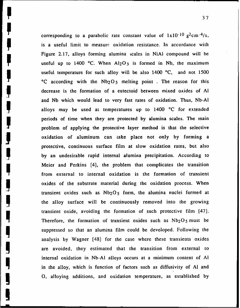
* 37
corresponding to a parabolic rate constant value of lxl0-10 g2cm-4/s,
is a useful limit to measure oxidation resistance. In accordance with
Figure 2.17, alloys forming alumina icales in NiAI compound will be
useful up to 1400 *C. When A1203 is formed in Nb, the maximum
useful temperature for such alloy will be also 1400 'C, and not 1500
'C according with the Nb205 melting point . The reason for this
decrease is the formation of a eutectoid between mixed oxides of Al
and Nb which would lead to very fast rates of oxidation. Thus, Nb-AI
alloys may be used at temperatures up to 1400 *C for extended
periods of time when they are protected by alumina scales. The main
problem of applying the protective layer method is that the selective
oxidation of aluminum can take place not only by forming a
protective, continuous surface film at slow oxidation rates, but also
by an undesirable rapid internal alumina precipitation. According to
Meier and Perkins [4], the problem that complicates the transition
from external to internal oxidation is the formation of transient
oxides of the substrate material during the oxidation process. When
transient oxides such as Nb20 5 form, the alumina nuclei formed at
the alloy surface will be continuously removed into the growing
transient oxide, avoiding the formation of such protective film [47].
Therefore, the formation of transient oxides such as Nb 2 0 5 must be
suppressed so that an alumina film could be developed. Following the
analysis by Wagner [48] for the case where these transients oxides
are avoided, they estimated that the transition from external to
internal oxidation in Nb-Al alloys occurs at a minimum content of Al
in the alloy, which is function of factors such as diffusivity of Al and
0, alloying additions, and oxidation temperature, as established by
U

38
TNFPKRATURgC- oc.•2000 Igoe 1600 14100 ].200 lose goo
WZIGUIT GAIN AT-310-10 qZCU"4$@C-1 -
100 he - 6 u/CU2
1000 he o - 19 /caZI -h . 60 ftq/CU2
-6
UbUA
00 -9
-10 ,- S0OC 1750 2S O OC LIMIT
I10 -1Sir
-13 .A1203 (NLt
-14S04 7 1
ýxoU 0- W
Figure 2.17 Parabolic rate constant vs Temperature for
oxidation resistance materials [46].
III

39
the following equation:
IBN0AI > [( (g*/3)" NO(s) (DoVm)/(DA1Vox) ]1/2 .......... (2.9)
which encourage the formation of the alumina at lower aluminum
compositions in the alloy by an increase in the aluminum diffusivity
and a decrease in the solubility and diffusivity of oxygen. Estimations
made by Perkins and Meier [41 indicated that it is very difficult to
form a protective alumina film on binary Nb-Al alloys at low enough
aluminum content to consider them still Nb-base. In accordance with
cbservations from other authors [49], the interdiffusion coefficient of
b.c.c. Nb-Al alloys has been found to increase considerably with
aluminum content, and the value reported by Bodrov and Nikolaev
(section 2.1.2) is probably an underestimate. It has been suggested
[50] that the probability of formation of an alumina external layer
would be enhanced by accelerating the diffusivity of aluminum by
means of the use of other alloying elements. In accordance with some
authors [4], an increase in the diffusivity of aluminum of about 2-3
orders of magnitude is possible if an extended b.c.c. solid solution
existed. The elements that increase the solubility of aluminum in
b.c.c. Nb are titanium, iron, chromium and vanadium.
The solubility of oxygen in the Nb-based alloys can be
suppressed by the additions of alloying elements by the gettering
effect of these elements. As mentioned in the previous section, Ti is
one of these elements which, in addition, forms an oxide that has a
desired stability between A1203 and Nb oxides. As explained by Lauf
et. al. [51], the addition of 1-5% of solutes such as Ta, Ti, V, or Zr to
Nb-based alloys decreases the 0 diffusivity significantly.

I 40
The topics of internal and external oxidation of alloy solutes
Shave been studied extensively [50, 52, 531. It is clear from these
investigations that oxidation protection can be obtained by means of
complex mechanisms that involve the diffusivity of 0 into the metal
I substrate to form oxide particles or films that require a solute to
diffuse out such substrate. Titanium would appear to be a probably
effective addition for increasing DAI and decreasing Do and No in Nb-
based alloys. Additions of 20% Ti should nearly double the solubility
of aluminum in niobium at 1400 "C as it forms a continuous b.c.c.
solid solution with niobium which can dissolve 42-48 at.% of
aluminum at 1400 *C [41.
2.2 Diffusion Theory and Mechanism
2.2.1 Binary Diffusion
I When two different components are placed in contact and
allowed to interact at a moderate temperature, thermodynamics
predicts that a variety of compositions and phases may form. Under
adequate experimental circumstances the interaction between the
two components, so-called Diffusion, eventually would lead to the
reproduction of all the phases between the end compositions.
Diffusion is defined as the movement of atoms in a solution as a
consequence of an initial chemical potential gradient, usually
expressed as a composition gradient, which the thermodynamically
unstable system try to eliminate by going to its lower energy state
(equilibrium). When the interaction between the two components is
conducted in single phase, the matter will flow in a manner that will

41
decrease the concentration gradient with the net flow of matter
ceasing when no chemical potential gradient exists anymore , that is,
when homogeneity in the system is reached. Specifically in solids, the
diffusion is conducted by either a vacancy mechanism (substitutional
solid solutions) or interstitial displacement of solute atoms
(interstitial solid solution) depending on the size difference between
the solute and solvent atoms making up the solution. Next, a brief
analysis of the fundamentals of the theory of diffusion for the
diffusivity, mostly in substitutional solid solutions, is presented.
2.2.1.1 Pick's Laws of Diffusion
Adolph Fick [54] proposed in 1885 an equation that fitted the
fact that the flow of matter of component i, Ji, across a given plane
goes to zero as the system reaches equilibrium, i.e., the concentration
gradient vanishes:
Ji = - Di [aci/ax] (i= 1,2) .......... (2.10)
where ci is the concentration If component i, and x is the distance
taken parallel to the concentration gradient of such component. The
proportional factor in equation 2.10 is known as the coefficient of
diffusion (or simply diffusivity). Originally D was conceived as a
constant at a fixed temperature, which later on was proved to be
true only for gas solutions.
Equation 2.10 is valid only whc.n the considered system is
under steady state conditions (no concentration changes in a point
with time). To take into account the variation of composition with
.I. ...

r- 42
U time, Fick's first law is inserted into an equation describing a local
3conservation of mass. "Ii,. Fick's second law can be expressed as:
dci/dt = divJi = -div [ -D Vck. .......... (2.11)
3 This equation has the properties of a continuity equation and stems
only from the conservation of matter. There are two classical
solutions to Fick's second law, which are discussed here.
a) D constant. steady- and non-steady states
If D is independent of position equation 2.11 can be expressed
as
dci/dt = D V[Vck] ==D V2ck .......... (2.12)
where V2 is the LaplacianV2 = a2 lax,ay,az .......... (2.13)
if a steady state exists, dcldt equals zero. Assuming the simplest case
(unidirectional diffusion) equation 2.12 reduces to D . (dc/dt)= 0. This
case does not occur very often. When the diffusivity is not a function
of composition (or position for that matter) but non-steady state is
acting, equation 2.11 is expressed as:
dc/dt = D a2c/ax2 .......... (2.14)
A solution to this equation will express the concentration of a
component i as a function of position and time, c(x,t), under the
-I adequate initial and boundary conditions. In the case of semi-infinite
solids:I c(x,t) = C'/2 [1 + erf (x/2Dt) .......... (2.15)
where c'=initial solute concentration of the richer side in component iz
erf= error function= (2/,4,) f exp (-u2 ) du0

* 43
1 1b) The Boltzmann-Matano Method
The coefficient of diffusion varies with composition in real
experiments. The dependence of D on composition forces the Fick's
I, second law to be written as:I aci//at= - a [Di(aci/ax)] /ax .......... (2.16)
This is an inhomogeneous differential equation, which its solution is
extremely difficult in the best case. The most common solution
employed in metallurgical studies on diffusion is the so-called
I Boltzmann-Matano analysis, which allows D to be calculated from a
concentration profile plot. This method is based on a solution of Fick's
second law proposed by Boltzmann [55] in 1884 and was proposed
for the first time by Matano [56] in 1933. After a diffusion couple
has been prepared and annealed at a fixed temperature during a
time t the experimental concentration-penetration curve c(x,t) is
experimentally determined (e.g. microprobe analysis). The resultant
curve should not be necessarily symmetric and in that case an error
function solution can not be applied. A solution to equation 2.16 may
be obtained by applying the so-called lamda substitution X [571:
I = Xlqt .......... (2.17)
which can convert the partial differential equation 2.16 into a total
, differential equation relating c and the variable X. This
transformation results in:
-[ /2] dc = d[D dc/dX] .......... (2.18)
Equation 2.18 is constituted only by total derivatives since c is only
function of X. Integrating 2.18:
II

* 44
I C C C
"-f X/2 dc = J d [D dc/dX] = [D dc/dXI I .......... (2.19)I C- C- C-
where c-=original composition (constant)
I c= variable composition at point A (or xt"112 )
= D(c) dc/d. - D(c.) dc/dX ....... (2.20)
Arranging 2.19: D(c) = [ - /2 dc] [ dX/dcl .......... (2.21)
Differentiating equation 2.17 at a fixed time gives:
dX. = dx/t-1/2 .......... (2.22)
Substituting in 2.21 yields:C
D(c) = -1/2t (dx/dc)c f x dc .......... (2.23)C-
This solution requires a proper evaluation of the x= 0 point
corresponding to the original interface, which may be evaluated by
applying a conservation of mass condition. A procedure to locate the
original interface from the composition profile considers Figure 2.18.
The total area under the curve is given by:*CJ c(x) dx .......... (2.24)C-
The plane at which x=O, so-called Matano interface, is determined by
finding the valae uA x in the diffusion zone (xo) such thatC C C
fJc.dx =Jfc+ dx =c(x) dx ...... (2.25)C- C- C-
Graphically, the Matano interface is the line that makes the two
hatched areas in Figure 2.18 equal. This figure also presents a sketch
of the area under the curve (fxdc) and the inverse of the slope dxldc
as a function of composition (position). Note that 'the Matano
I

p 45
1.0
0.8
_0.6
M--notano Interface
O.c Tonqmn,-
0.4-
10.:
-I
Figure 2.18 Typical composition profile of an annealedI diffusion couple. The Matano interface is
positioned to make the hatched areas ,n (crosshatched area), and the tangent values employedto calculate the intertdiffusion coefficient at acomposition c= 0.2-co.

46Iinterface is characterized by a maximum at the area under the curve
and a minimum in the inverse of the slope. The error in the
p calculated D is largest at the ends of the curve where c-Ic +
approaches zero or one as in those regions the integral is small and
dx/dc large. As mentioned before, the Matano-Boltzmann method is
widely employed in metallurgical diffusion studies as it is very
useful for determining D over a range of compositions in alloys.
Among its advantages are the wide availability and development of
both electron analysis techniques and computers, which make this
procedure highly automated. However, one detriment in the
procedure is that equation 2.23 assumes that the atomic volume ofproedureo is thteutoi.3asm s ta h atslomi volue. o
the alloy is independent of composition, which is a seldom case.
2.2.1.4 Binary Diffusion by a Vacancy Mechanism. The Kirkendall
Effect and Darken Analysis
Two mechanisms have been proposed to explain diffusion in
substitutional solid solutions. The first is the cooperative movement
of atoms. Zener's ring or direct interchange, described later in this
section, are examples of this mechanism. However, energetic
considerations and the fact that the Kirkendall effect occurs, ruled
out these mechanisms as possible ways for substitutional diffusion to
occur. The second kind of mechanism implies the movement of a
single atom at a time, and the example is the universally accepted
mechanism of vacancy diffusion. In this case, the atom of an adjacent
site simply jumps into the vacancy, but for that to happen, a small
displacement of the neighboring atoms is required, which constitutes

47Ione of the energy terms required for diffusion encountered in the
I expression:
D= a a2 Z u exp-(AGm + AGf)/RT .......... (2.26)
where Z= coordination number
I a= lattice parameter
a= crystallographic geometric factor
u= vibration frequency of a solute atom in an interstitial site
AGm= free energy per mole needed for solute atoms to jump
I between interstitial sites.
I AGf= free energy term per mole associated with the formation
of vacancies.
I pre-exponential factor is fairly constant with the temperature
and can be joined in a single term called frequency factor Do.
I Knowledge of the operating mechanisms of diffusion in b.c.c.
materials is not as extended as that for f.c.c. metals. Self-diffusion
and impurity diffusion in b.c.e. metals occurs via vacancies. In a b.c.c.
lattice the barrier for the jump of one atom into a neighbor vacant
site is more complex than it is in f.c.c. structures because of the
saddle point barrier with double maxima in energy that the hopping
atom must overcome [581. Fritzsch et. al. [59] studied the diffusion
via vacancies as the dominant mechanism in b.c.c. metals by
calculating the parameters of a given interaction, such as the
influence of lattice constant and binding energy, between the atoms
and the lattice. They considered three types of jumps as exemplified
in Figure 2.19, and calculated their potential curves (Figure 2.20),
which show that the jump to the next nearest neighbor type A is
favored due to the smaller distortion in the hopping event. They

48
o 0-a b Jc
Figure 2.19 Atomic jumps in a b.c.c. crystalconsidered in the model calculationmade by [59]. a) Type A: jumps to thenearest-neighbour position, b) Type B:jumps to the second nearest-neighborposition, c) Type C: jumps to the thirdnearest-neighbour position.

49
-- S
0 a5 TD.p_.Wiion -
Figure 2.20 Potential barriers for the cited types ofindividual jumps starting at r= 0 andending at r= 1. The maximum value ofeach curve corresponds to the migrationenergy for the particular hopping event[f9].

50
found a strong proportionality between migration energy and the
binding energy of the crystal for the self-diffusion case (Figure 2.21),
which is in good agreement with published experimental data. As to
the impurity diffusion case, it was concluded that the bigger the
impurity atom, the higher would be the migration energy, which also
agrees with experimental data presented by Tiwari et. al. [60]. The
binding energy found by [59] has only a small effect in this migration
energy.
Regarding with the soluLion to the diffusion equations
presented before, it should be pointed out that the Matano-
Boltzmann solution gives only one diffusion coefficient, D, that
completely describes the process. In this kind of experiment, the
coordinate system employed is fixed relative to the ends of the
specimen, and it is observed that the diffusivity gives rise to the
movement of one part of the diffusion couple relative to the other.
Therefore, ahy movement of lattice planes relative to the ends of the
couple is recorded as a flux and affects D (equation 2.10), even
though such translation does not correspond to any jumping of atoms
from one site to another. Since the process takes place in a chemical
concentration gradient the resultant D represents the cnemical
diffusion coefficient, also called the interdiffusion coefficient. For the
complete description of the diffusion behavior of binary
substitutional solid solutions, however, at least five different
diffusion coefficients are needed for each concentration, namely:
D= interdiffusion coefficient
DA,B= intrinsic diffusion coefficients of A and B components
D*A,B= tracer diffusion coefficients of A and B components

* 51
I
I • 00, -00
UA86 7
".1/o
Figure 2.21 Migration energy for self-diffusion independence on the binding energy ofU the crystal in comparison with theexperimental data refered therein. Theline drawn presents the calculated
relation by [59].
/,,I•o/ ',
I."I/ °,
* 52
The tracer diffusion coefficients arises from the fact that studies
showed that the self diffusion coefficients [61] are in general
different for the two elements. In self-diffusivity studies one studies
the diffusion of a radioactive isotope solute in a matrix of the same
p (non-radioactive) metal. Except for a small mass difference, the two
atomic species are identical. This mass difference permits to calculate
the jump freq'iency of the isotope and a self-diffusion coefficient,
which for b.c.c. metals is given by:
Db.c.c. = a2 /8• .......... (2.27)
where r is the dwell time of an atom in a lattice position. Thus, a
relationship between the chemical diffusion coefficient and the self-
diffusion coefficients must be found. Such relation was brought about
in 1947, when Kirkendall and Smigelskas [7] conducted diffusion
experiments on diffusion couples formed by a rectangular bar of 70-
30 brass plated with 0.1 inch of copper. The original feature of their
work was the incorporation of Mo wires in the interface of the two
materials as markers (Mo is insoluble in either Cu or Zn). After
annealing, a thin slice of the couple was cut and metallographically
3 prepared to measure the distance between markers. The experiment
was repeated at different annealing times. In all cases was found
that the markers distance decreased an amount proportional to the
square root of the annealing time, even after subtracting the small
volume change in adding Cu to brass. The only way to explain this
3 markers shift was that each of the two atomic forms moved with
different velocities, i. e., that the flux of Zn atoms outwards across the
markers plane be much larger than the flux of Cu atoms inwards
I

* 53I
across the same plane. Later work in different systems prove the
* generality of this concept.
The Kirkendall effect can be taken as a confirmation of the
vacancy mechanism of diffusion in cubic materials (f.c.c. and b.c.c.).
As mentioned earlier, another possible diffusion mechanism in
substitutional solid solutions of b.c.c. metals is the ring mechanism
proposed by Zener [62). Here, the energy needed for diffusion is
smaller due to a more open structure; however, experiments on
I many diffusion couples composed of a number of different b.c.c.
metals showed that a Kirkendall effect occurred. Interchange
mechanisms such as the ring one require that the rate at which
3 atoms of A move must equal the rate at which B atoms move in the
other direction. Consequently, no Kirkendall effect would be
* observed.
Kirkendall's experiment showed that the atoms of two species
in a diffusion couple move at different rates. Thus in accordance with
this concept, the interdiffusion coefficient previously defined should
be used only to describe the flow of components relative to some
* component averaged convective velocity and basically is the same
for components A and B. Kirkendall experiment showed that using
the right reference frame for the motion of the atoms, one can get a
* different result for the diffusion behavior of each of the components
and talk about a behavior which is intrinsic to each of the
* components.
In 1948, Darken [63] published an excellent phenomenological
analysis of diffusion of alloys based on such experiment. He
5 contended that the markers motion was due to an imbalance of flows
'I

5 54
of the two components, and that each component had a flow of rate
of his own, bringing along the definition of intrinsic diffusion
coefficients. Consider Figure 2.22 and define VL to be the local
velocity of the lattice during interdiffusion. In the Kirkendall
experiment, after some annealing time, the markers plane will move
in the positive direction. If markers are placed in all the couple,
those in the diffusion zone will move in a different extension. In the
comers there will not be movement and VL= 0, whereas in the
S middle (interface) VL will be maximum. From his analysis, Darken
derived two equations. The first one:
VL=[-DB + DA] (OXA/ax) .......... (2.38)
permits to obtain the Kirkendall velocity at any point. For example,
at the comers of a semi-infinite diffusion couple, dXAIdx equals zero,
and then VL=O, whereas at the interface the local gradient will be
maximum and VL will be maximum too. The value vL can be
measured experimentally by measuring the velocity of the markers
and the local concentration gradient by microprobe analysis. The
other Darken's equation can be expressed as:
D D=XBDA + XADB .......... (2.39)
Again, D can be determined experimentally by the Boltzmann-
Matano method. To obtain DA and DB at a given composition one
needs to determine the markers velocity and the interdiffusion at
the position in the couple where the markers reside. From the
composition profile obtained, for instance, by microprobe analysis
the variables XA, XB, and dXA/dx can be determined at that point.
Then by solving simultaneously equation 2.38 and 2.39, the intrinsic
diffusion coefficients can be calculated:
I

p 55
I/Co+0II
/. 0
F It
I (*1
U ICC~:i_ _

P 56
DA = D + XA VL [1XA/a}x]........................ .......... (2.40)9DB = D +XB VL [aXB/aX]
9• 2.2.2 Ternary Diffusion
9[ The analysis of a diffusion process in multicomponent systems
(ternary or higher order) is rather complicated. Even in the most
common case (temperature and pressure constant, no external force
fields) the appearance of diffusion flux of any component is able to
cause diffusion redistribution of all the other components. As to the
effort needed, in general the amount of experimental work required
increases approximately as the square of the multiplicity of the
system. In order to alleviate the complexity of the analysis, "the
experimental approach of ternary systems must be accompanied by
an exhaustive theoretical investigation of all aspects of the problem"
[641. In this section a brief review of the formal elements of the
ternary diffusion theory in single phase substitutional systems is
presented. For the sake of simplicity during the analysis possible
effects such as volume changes of mixing, lateral dimensional
changes and pore formation will be neglected.
2.2.2.1 The Diffusivitv Matrix
At present the most common method to define the total set of
mutual diffusion coefficients in multicomponent systems is that of
Matano-Kirkaldy [64]. A brief explanation of its fundaments follows.

p57
As in the binary case, the flux equations may be written in terms of
either the chemical potential gradient (cal/mole) or the concentration
gradient (mole/cm 3 ) in the Kirkendall (lattice fixed) frame of
reference. Generally, the flow equation (Fick's First Law) for this case
p] is:
Ji= I [D ij ]Vcj .......... (2.41)j-2
where [Dij] is known as the matrix of diffusivities. Note that j runs
from 2 to c in this equation. In a ternary system there are two
independent composition variables. Therefore, a diffusion couple
p experiment requires the determination of two independent
composition profiles to characterize a couple. Since to a good
approximation:
c I + c2 + c3 = c (moles/cm 3 )= constant .......... (2.42)
and its derivative:
IVl + Vc2 + Vc3 = 0 .......... (2.43)
then, the dependent variable:
Vc 3 = -(Vcl + Vc2 ).......... (2.44)
Regarding with the index i in the equation 2.41, it runs only over two
components because the 3 fluxes are not independents:
J Jl+J 2 +J 3 =0 .......... (2.45)
From Gibb's phase rule, ternary systems offer an extra degree
of freedom as compared to binary couples. This fact means that the
sequence of compositions (so-called composition path) in ternary
systems may be different from couple to couple in the same system.
.1 Such composition path is time invariant for semi-infinite couples and
is represented by a continuous curve on the Gibbs triangle ternary

P 58
phase diagram representation that connects the endpoint
compositions of the alloys making up the diffusion couple (Figure
2.23).
When the dependent variable is component 3, equation 2.41
can be expressed as:SJ 1 = - D11 •3 c /x - D12
3ac2/ix.......... (2.46)
J2 = - D2 13jl'&ix - D22
3ac2//xpOne problem associated with the definition of the diffusion
coefficient in a ternary system, however, is that it depends upon the
choices made for the dependent flux and concentration gradient; so,
the same equation 2.41 can be rewritten as (using short
nomenclature):Jl = - DII 2VCl - D 13
2Vc3........... (2.47)
J2 = - D 2 12 Vcl - D 23
2 Vc3
when component 2 is the dependent variable. Substituting 2.44 in
2.47:
J= D112 VCI - D 13
2 (-VCI - Vc2 )
J2= - D 2 12 VC1 - D 2 3
2 (-VCI - Vc 2 )p then, Jl = - [D112 - D13
2 ] VC, - D132 (-VCl - Vc 2 )
..................................(2.48)
J2 = - [D212 - D23
2 ] VC, - D 232 (-VCI - Vc 2 )
comparing with 2.46:D 1 1
3 = [DII 2 - D 132 ]
D 1 23 = - D132
I= 1 D .......... (2.49)D2 1
3 = [D 212- D23
2 ]
D 223 = -D232
These relationships among the coefficients of diffusion lack physical

59IIIII
I (C I C / ( ci7c*
j (c,.)
COMPONENT L
II Figure 2.23 Composition Paths in a ternary system isotherm.

60
meaning, and a result such as DII>D22 may not necessarily imply that
component 1 moves faster than component 2 in the system.
In equation 2.46, the on-diagonal element (i=j), known also as
the mutual diffusion coefficients, reflect how the gradient of
component iinfluences the flux of the same component. The so-called
off diagonal terms (or indirect coefficients) report how the gradient
of the other components affect the flux of the component i.
Frequently, the off-diagonal terms are much smaller than the on-
diagonal terms.
2.2.2.2 Experimental Determination of [Diil. The infinite Diffusion
As in the binary case, the infinite diffusion couple is one of the
most useful techniques to obtain solid-state ternay diffusion data
because the associate boundary conditions leads to a particular
rather simply integrals of the diffusion equation. For instance,
applying local conservation of mass on equation 2.46 it is possible to
derive the equivalent of Fick's Second Law:
ac l/at= a(D• ac 1/ax)/ax + a(D 123 ac2/ax)/ax
.......... (2.50)ac2/at= a(D 21
3 ac /ax)/ax + a(D 22 'c2/Iax)/ax
subject to the boundary and initial conditions:
Ci(± X, 0) = Ci(± 00, t) = Ci+ ....... (2.51)
As in the binary system, in this case it is possible to make the lamda-
substitution (equation 2.17), and convert the partial differential

61
equation 2.50 into a total differential equation, which after the
Matano-Boltzmann solution yields:
- (I/20 f X dcl = Dii3 dci/d). I + D123dc2/dX I.......... (2.52a)
ci.- c1Q.) c20.)
similarly,c2(.)
-(1/20 f X. dcl = D2 13 dcl/d. I + D22
3 dc2/d. I.......... (2.52b)
C2- cIO() c2(.)
The left side of equations 2.52 can be empirically evaluated with the
composition profile of each component (Matano Integral). This is
graphically illustrated in Figure 2.24. Then for a particular
composition, the information needed to evaluate equation 2.52 is
PAdc, obtained by a numerical technique, and the slope of the curve
at that composition point, which can be readily obtained. Thus, at any
composition there are two simultaneous linear equations with a set
of 4 unknowns: D11, D1 2 , D2 1 , D2 2 . To make the system determinate,
therefore, it is necessary to produce another independent diffusion
couple and perform the same analysis on its composition profile.
Consider Figure 2.23. If the diffusion couples have been chosen
so that their compositions paths on the ternary isotherm cross at
coordinates (c,,c 2), we see that there are 4 equations and 4 unknowns
soluble only at that concentration (c,,c 2) which is common to both
couples; the values of the set of form D ij's, being functions only of
compositions but not the gradients, will be the same for that
composition that appears in both couples. Thus, the bottom line is
that the matrix [Dij] can be determined by the Matano-like analysis
in two diffusion couples at their crossing points, over which no

62
A B
I I
''t3
C 2
__....IC_ 7€2/$6t
Figure 2.24 Evaluation of Matano integrals and slopes at a givencomposition for evaluation of diffusion coefficients internary systems.

63
control exists. One problem associated is that the crossing point
composition is usually one end of the composition path which makes
no easy the evaluation of the integral and slope, diminishing the
precision of the result. Then, the general strategy employed in
experimental studies generates a whole collection of diffusion
couples that survey the ternary region to be studied. After
determining the resultant composition profiles and their
corresponding composition paths, the integrals and derivatives are
evaluated at all crossing points that happen to develop between pairs
of couples. It should be pointed out that a given couple could have a
lot of intersections with other couples. The results of this kind of
study are usually reported as a counter map of each of the diffusion
coefficients: D11, D12 , D2 1 , D22 as a function of composition on the
Gibbs triangle (Figure 2.25) [65]. These values are far from the real
physical meaning, so that if Dll>D12 that does not mean necessarily
that component I moves faster than component 2. The interdiffusion
studies in Cu-Ag-Au system by Ziebold and Oglivie are a typical
application of these strategy [65].
The amount of experimental work required to survey the 2-
dimensional surface of the Gibbs' triangle for each Dij can be reduced
drastically by the use of special procedures and theoretical
knowledge about the diffusivities. Special procedures for evaluating
the 3 independent mutual coefficients have been described by [66-
681.
Some important experimental tendencies in typical ternary
studies indicate that the maximum in D occurs usually close to the
corresponding value of the minimum melting point. Another

64
GOLD. INTERSECTIONe EXTREME
20 %se 2 0IV
% % , f ,
I,
90 so
00
COPPER SILVER
Figure 2.25 a) The direct coefficient of diffusion for Cu D113in units 10-12 cm21sec at 725 OC. Filled circlesindicate intersections of diffusion paths. and
open squares indicate extreme points in thecomposition profile [651.
I | A

I 65
5 GOLD
"" INTERSECTION"" EXTREME
q .O 20 20 %
:•' ^•" /0 8" , 160 I), -
I FiueC2.Cniue.)Tedrc offceto ifsoCOPPR SLVS
(J 66333 130% -
q .4.,
A9 G 60 ir1 A.0
80 so
COPPER SILVER
Figure 2.25 (Continue) b) The direct coefficient of diffusionfor Ag D22 3 in units 10-12 cm 2/sec at 725 0C.Filled circles indicate intersections of diffusionpaths, and open squares indicate extreme pointsin the composition profile [65].
III
I
66P interesting observation is that to calculate D, jfrom extreme values
(maximum or minimum) in the composition profiles, we do not need
a crossing point since the Vcij equals to zero at that particular
concentration reducing the equations 2.46 to a system of 2 equations
and 2 unknowns:
J1= - Dli 3acl/ax - D12 3 &c2/ax = - Dli 3 acl/ax
... (2.53)
J2!= - D21ae /ax - Dz23 c2/ax = - D213 e I/lax
5p 2.2.2.4 Diffusion Penetration Tendencies and Composition Path
Patterns
In 1974, DeHoff et. al. [69] published a new viewpoint on the
analysis of the diffusion behavior in ternary systems where [Difj is
replaced by the relative penetration tendencies of the 3 species.
Through this approach, the calculation of a complete pattern of
composition paths and Kirkendall shifts on the Gibbs triangle for the
relative penetration tendencies of the components is relatively
simple.
During their analysis, they made 3 assumptions. First, the
interpenetrations of the species occur on a rigid lattice so that
appreciable excess and deficit of atoms can occur on one side and the
other. To do this, the normal continuous feedback of vacancies was
changed for a one-step feedback that permitted the readjustment of
the lattice. This was recognized as physically unreal, but essential for
the calculation of the Kirkendall shift for the system. The third
element of the approach was approximating the concentration-
I1

P 67
penetration curves for each component as straight line with the rigid
lattice as the coordinate system. In this case, when the depth of
penetration of an element depended on composition, the
concentration-penetration curve was approximated by two straight
line segments.
Consider a diffusion couple made up by alloys A-50at%B (P
side) and B-50at%C (Q side) in a single ternary system A-B-C whose
relative penetration depths are independent of composition and
already known: AŽ_B_ŽC. Figure 2.26a shows the linear composition
profiles (in atoms/cm 3 ) for this couple in a rigid lattice before and
after the diffusion treatment. In accordance with the relative depths
of penetration, component A draws deeply from the P side of the
couple and penetrates deeply in the Q side of the couple. Regardless
of its mobility, component B does not move since no concentration
gradient for it is present. Component C slightly penetrates into the P
side and draws from a shallow depth on the Q side. The total
concentration of atoms in the unshifted lattice (Figure 2.26b),
obtained by adding the number of atoms of the 3 species point by
point, clearly shows a deficiency of atoms/cm 3 in the P side and an
excess of them in the Q side. Since co is considered to be independent
of composition, it is necessary to generate a nur-ber of vacancies
proportional to the area A I in the right side, which in turn will
increase the thickness of the Q side and decrease the P side of the
couple. This unbalance will produce a Kirkendall shift (translation of
the original weld interface) toward the left side of the couple, shown
as Xk in Figure 2.26c. Since all the positions in the diffusion zone are
shifted by this process, the original coordinate system x- (rigid
I

P0 68
p _ _ _ x •
P Io I x
m V
c C
a)
CT O A2ý
Co
I o C
C)Co *
P
Figure 2.26 a) Model for a ternary diffusion couple with independent
concentration penetrauon tendencies; b) total concentration curve;
c) computation of Kirkendall shift: d) prediction of Kirkendall
shift: e) atom-fraction penetration profiles for the unrelaxed
Ilattice; and f) computed composition path [69).latc:adI optdcmoiinpt 6)
I

69
lattice) is transformed to a new coordinate system x which is all
moved to the left. The magnitude of this change, however, is
different in different positions. For example, at xj0this magnitude is
proportional to the volume change accumulated to the left of this
point by the annihilation of vacancies (area A3), which must be equal
to the to the volume occupied by these vacant sites prior to their
annihilation (area A4). By equating these two areas at each point of
the affected lattice, it is possible estimate the magnitude of the
lattice displacement of the original system, Ax. Note that the
Kirkendall shift is maximum at the weld interface (Figure 2.26d).
The atomic fractions of XA, XB, and XC are shown in Figure
2.26e. They are derived at any point of the unshifted system by
dividing the corresponding ci by the respective ct. This curves would
be the experimental result given by the microprobe analysis.
Observe how the profile corresponding to the component B varies up
I and down as it crosses the diffusion zone suggesting a movement of
3 atoms B from the right side of the couple in a possible uphill
diffusion way. However, as mentioned earlier there is not effective
flow of atoms B at all because of the absence of a B concentration
gradient, and the variation of its composition is due only to the
U !imbalance in the distribution of A and C atoms. Finally Figure 2.26f
shows a plot of the composition path and Kirkendall shift that would
be observed for this kind of system. There are some interesting
observations that should be noted in this plot. For example, the two
ends of the path point directly toward the corner of the fastest
component A, and the central part of the path tends to point toward
the corner of the slowest component C. This causes a considerable

I 70
deviation of the composition path from the straight line joining the
endpoint compositions (concentration tie-line) with the path curve
crossing at half way of this tie-line. The intersecting point is called
the cross over-point and is important in the determination of the
Kirkendall shift.
When the mobility of the atomic species in the couple varies
with composition, the depths of penetration and draw for each
component are different on the 2 sides of the couple. This case is
illustrated in Figure 2.27 [691. The only difference with the previous
case is that the penetration and draw depths are larger in the left
side of the couple (richest in the fastest component A) and more
shallow in the other side. The determination of the concentration at
the welded interface is given by the fact that the triangular areas on
both sides of the couple must be equal for each component
(conservation of atoms). A similar analysis to that given above would
explain the plots for this case. Nevertheless, some interesting
deviations in the composition path for this case must be mentioned.
One is the displacement of the crossover point toward the P side of
the couple. An important characteristic of the crossover point is that
its composition correspond to that of the original weld interface. The
Iother difference is that the penetration curves are skewed, which
causes an enlargement and a shortening in the the length of the
segments at the end of the composition path in the P and Q side,
respectively.
This approach was successfully applied by the authors to
generate simple penetration tendency models that reproduce

71
P X , P c i
x Xx
- C
C r
T
I
AX
IkI xC
a)
Figure 2.27 a) Model for a ternary diffusion couple with concentration dependent
penetration tendencies. b) total concentration curve; c) computation ofi Kirkendall shift; d) prediction of" Kirkendall shift. e) atom-fraction
penetration profiles for the unrelaxed lattice. and f) computedcomposition path. Note the ondulation in component B (e) and the
i ~displacement of" the crossover point on the path (f). [691
I • T

T 72
I experimental composition paths and Kirkendall shift patterns in
different ternary systems, such as Cu-Ag-Au, Cu-Ni-Zn and Cu-Ni-Zn.
2.2.2.3 Zero Flux Plane
I In 1979, Dayananda and Kim [70] described a different way to
calculate interdiffusion fluxes in binary and multicomponent systems
directly from composition profiles of isothermal diffusion couples by
an analysis directly derivable from the continuity equation without
the need for a prior knowledge of interdiffusion coefficients, the only
IJ assumption being constant molar volume. A major outcome of their
interdiffusivity studies on the Cu-Ni-Zn system was the identification
of 'zero flux plane' for each component within the diffusion zone of
the diffusion couples. They defined a 'zero flux plane' as the plane
where the interdiffusion flux of a component goes to zero and on
I either side of the plane occurs a change or reversal in the direction of
the interdiffusion flux of the component.
.iI
I

CHAPTER 3MATERIALS AND EXPERIMENTAL PROCEDURES
In this chapter a description of materials and experimental
techniques employed throughout this research is given. A flow chart
that represents the experimental procedure for preparation and
analysis of diffusion couples is given in Figure 3.1. The experimental
procedure consists of alloy preparation by arc-melting,
homogenization, diffusion couple preparation, interdiffusion heat
treatment, analytical analysis using microprobe, and computerized
analysis of the composition profiles. These steps are explained in the
following sections.
3.1 Materials
The alloys used in this study were prepared by arc-melting of
high purity materials (99.99% Nb and Ti, 99.999% Al). The pure
metals were in the form of a 5-mm-thick niobium sheet obtained
from Teledyne-Wah-Chang, a 6.35-mm-diameter titanium rod from
Aesar, and a 38-mm-diameter aluminum rod from United Mineral
Corporation. Table 3.1 gives the ingot analysis of the pure metals.
1 73

74II
I -"
I 0 -0
I 6.
o •to
C06,
I _- <I
00.
I <-5m
I -
OM.
1 1A

75
Cu V - .
.C
0E
COw
CLu
E c
U C
0
~v
E Z
"- Z V) ,
"2. C
•,. ,.,

76
3.2 Alloy Preparation
The binary and ternary alloys were prepared by arc melting
weighed amounts of pure metals on a water-cooled-jacket copper
stage under an oxygen-gettered argon atmosphere. Before melting, a
vacuum of 100 mtorr in the chamber was attained and then argon,
previously dried in a gettering furnace was allowed into the system
up to a pressure of -15 KPa. The purging operation was repeated at
least 4 times before proceeding to melt. The specimens were melted
under an Ar pressure of -35 KPa. Each specimen was melted at least
4 times to assure compositional homogeneity of the buttons. The
buttons were weighed after each melting operation so that Al losses
could be monitored. Weight losses were detected only in buttons of
the binary Nb-Al alloy and accounted for approximately 25% of the
initial Al weight. In order to obtain the desired composition in the
alloy, an excess of pure Al, equivalent to these losses, was added to
the samples before melting.
After metallography preparation, the alloys were analyzed by
microprobe analysis, whose results proved that the Al-loss
estimation was correct. The resultant compositions from the
microprobe analysis are shown in Table 3.2. In order to check their
accuracy, some of the alloys were sent out for wet chemical analysis.
Table 3.3 compares the results obtained by both techniques for the
binary alloy. A good agreement of results is observed.

77
I 00
tn 00 - 00 CNO 00-
0\0
cco tI* tn
U - - en~ en -

0
I., e-, .m
I-I

79
3.3 Preparation of Diffusion Couples
The arc melted buttons in the form of spherical cap-like shape
of approximately 3 gram weight and 8 mm height, were studied
using optical and electron microscopy. Microprobe analysis showed
macrosegregation and significant microsegregation in the
microstructure. Therefore, a homogenization of the alloys was
required. The buttons were plastically deformed to a disk-like shape,
5-mm thick, at room temperature using a press. The new shape
permitted to obtain flat surfaces and the plastic deformation
expedited the subsequent homogenization through breaking down of
the dendrite arms. All the heat treatments performed in this
research, i.e. the homogenization and the diffusion annealings, were
done in a Minivac Furnace Series 2400 Vacuum Bell Jar , which is an
ultra-high temperature vertical cold wall vacuum furnace capable of
temperatures up to 2000 °C. A schematic representation of the
furnace assembly employed for all the heat treatments is illustrated
in Figure 3.2 The pumping system, consisting of mechanical and
diffusion pumps and furnished with ionization gauges, is able to
produce a 10-6 torr vacuum in the bell jar. To prevent any
penetration of oxygen into the alloys during heat treatments, the
samples were wrapped in tantalum foil (100 gm thick). The binary
Nb-Al alloy (s00) proved to be also an excellent oxygen getter. Before
heating up the samples, a vacuum of 1E-5 was obtained in the bell
jar. The conditions for the homogenization treatment depended on
the chemical composition of the samples. In the case of binary alloy
P0o, the treatment was done at 1400 °C for 6 hours. For all other

I80I
102
I"
Cl
'00
p ___,__
E- Z
Cu fl ;
p Cu• rn ~
I o • ~i.-• l
:J•Lk-- I'I-LI
pp_- 7E. E. , , .- -

J 81
alloys, the homogenization was conducted at the same temperature
but for only 4 hours. The lower time is due to the presence of
titanium which reduces the melting point, and subsequently
increases the rate of diffusivity and the homogenization process. The
system was heated up to 950 'C for 30 minutes, and then brought to
the homogenization temperature of 1400 °C in 5 minutes. After
annealing, the samples were cooled down in the furnace. Optical
microscopy and backscattered electron analysis were performed on
the heat treated samples to ensure that the microsegregation was
removed and specimens were homogenized. Since an
environmentally affected zone, which is depleted in Al and has high
oxygen content, develops in the vicinity of the surface of the
homogenized specimens, the surface layer was removed and
rectangular specimens of (I x t x 0.5 cm 3) were cut from the
homogenized buttons. Samples were prepared metallographically for
the subsequent diffusion bonding using a fixture that permitted to
obtain parallel surface.
As mentioned in section 2.3, one of the simplest techniques to
assemble solid state diffusion couples is the window-frame technique
[71]. In this method, the two members of the couple are polished flat
and mechanically clamped together. In some cases, like in this study,
a short heat treatment at a temperature below the interdiffusion
heat temperature is used to facilitate the diffusion bonding. The use
of suitable markers to delineate the original bonded interface is
important. Their size should be small enough to avoid interferingI with the diffusion bonding process but big enough to be detected by
the SEM. They also should be chemically inert with the components
I

82
of the couple to avoid their decomposition during the heat
treatments. For this research, yttria (Y203) particles, 1 gim in size,
were employed.
The diffusion couples for this investigation were prepared
using a Centorr Series 600 Hot-Press Furnace. The steel chamber has
a workable space of 76 mm diameter x 127 mm high and is water
Jcooled by a flow of 5 GPM at 50 psi and 20 0 C. This system uses an
induction coil as a heater element to achieve temperatures up to
1500 °C in vacuum and neutral atmospheres. It is equipped with a
mechanical pump that permits to achieve a vacuum in the order of
1E-2 toff. For inert gas operations, inlet valves, relief valves and a
combination pressure-vacuum gauge are provided. To operate with
argon or any other inert gas atmosphere, the chamber can be
evacuated by means of the pumping system and then backfilled with
the desired inert gas. The specimens to form the diffusion couple
were compressed together by means of a hydraulic press with a steel
ram, 25.4 mm in diameter, coming down from the top of the
chamber. The temperature measurements were carried out by a fast-
respond optical pyrometer with adjusted chromatic compensation
and a precision of ± 10 °C.
Two kinds of diffusion couples were built for this research. For
the binary diffusion study a two-part couple was used, whereas for
the ternary diffusion case a sandwich-like couple was made. Small
drops of a dilute solution of the fine chopped yttria particles in
acetone were deposited as markers over the polished surface of the
specimens. The couple was compressed together inside a graphite
die. The 3-piece die consists of a stage where the sample to be
I!J

83
compressed rests, a ram through which the load is applied, and a
case to hold the whole system. Before setting the sample in the
graphite die, a very thin film of boron nitride, a very stable material
at the employed bonding temperatures, was sprayed over the faces
in contact with the specimen so that the diffusivity of the carbon into
the sample was prevented. In addition, a 100-ptm-thick tantalum foil
was placed between the boron nitride layer and the sample. The
whole system was then set into the induction coil in the chamber, as
shown in Figure 3.3. As in the arc melting operation, the chamber
was purged 5 times with gettered Ar before heating up the system to
the bonding temperature.
The diffusion couples investigated in this research are listed in
Table 3.3. The bonding temperature was 1030 ± 10 °C for the binary
diffusion system Nb(p)/130 and 930 ± 10 °C for the couples including
ternary alloys, except the couple made with pure Ti. Once at the
bonding temperature, a stress of approximately 2 MPa was applied
to the system and held for the length of the diffusion bonding. After
cooling down, the bonded diffusion couple was cut into two parts. A
section perpendicular to the bonded interface was metallographically
prepared for examining the quality of the bonded interface. The
characterization of the bonded interface prior to the interdiffusion
was done using optical microscopy, scanning electron microscopy and
microprobe analysis. A solution of Kroll's reagent (10 ml HF, 30 ml
H2NO3, 50 ml H20) was used as an etchant for revealing the
microstructure of the ternary Nb-AI-Ti alloys.

84
LOAD'I
GRAPHITE
DIE
TBoron Nitride-Tantalum Foil ••'-•- atlmFi
Cove r Tantalum FoilLayers Set
Diffusion Couple
Figure 3.3 Experimental set-up for hot-pressing bonding ofdiffusion couples.

85
'S -% % ' -3
7:3 ~ d
0 -A -u
<= I- 2 d-
I-V) -
- a - -- - - '
0 cr)
oý _n CO en
-ý r^ --
_-e 0 m c
0, - - - - M - - 0*~e 0n C11 00 0
o *- z z*. z-
m2 -t ~ tn % l- w0%
~ ei e '
u .~-~

86
3.4 Interdiffusion Heat Treatments
The diffusion couples were wrapped in tantalum foil, put upon
the alumina stage in the vacuum furnace, as shown in Figure 3.2, and
were surrounded by the Nb-Al binary alloy as a getter. A vacuum of
1E-5 torr was set in the bell jar before heating up to the
interdiffusion temperature. Again, similar to the homogenization
process, a short heating time (.5 minutes) from 950 °C to the
treatment temperature was registered. A close control of
temperature (±5 °C) was achieved by using a type C (W-5%Re)
thermocouple. Since the vacuum bell jar furnace lacks a quenching
capability, the samples were cooled inside the furnace. The cooling
rate, however, was fast enough to avoid further diffusion upon
cooling. For example, it took less than 90 seconds to go from 15500 to
950 °C, which is a n, )1igible time compared to the duration of the
interdiffusion treatments employed in this research.
To evaluate the diffusivity of aluminum in the binary Nb-Al
alloys, the couples (#1 to #5) were annealed for various lenght of
time in the temperature range of 1350°-1550 *C. The duration of the
heat treatment was limited by a lower bound sufficient to produce a
diffusivity zone of at least 25 gm at the lowest treatment
temperature, and an upper bound to avoid alumina formation in the
binary Nb-Al alloy at higher temperatures. Table 3.4 provides the
details regarding the binary interdiffusion treatments conducted.
With respect to the ternary system, diffusion treatments of the
sandwich-like diffusion couples were conducted at two different
temperatures (12000 and 1400 °C). First, diffusion couples #6 and #7

87
were treated at 1400 OC. Since the resultant penetration zone was
very large, the treatment temperature was decreased to 1200 'C. The
interdiffusion time for the ternary alloys was held constant (6 hours)
in order to compare the penetration tendencies in these couples.
3.5 Analytical Microscopy
The diffusion couples used in this study as well as the
materials employed during their construction were chemically
analyzed and structurally characterized by Microprobe Analysis
(EPMA), and Scanning Electron Microscopy (SEM) (Backscattering
Electron BSE and Secondary Electron SE modes), respectively. These
analyses were performed in the diffusion couples before and after
the diffusion treatment in order to check the extent of diffusion and
possible phase transformation during the bonding process, and to
obtain the respective concentration profiles for the diffusivity
analysis. Concentration profiles, were obtained using a JEOL
Superprobe 733 electron microprobe. This system is equipped with a
tungsten filament electron gun and four wavelength dispersive
spectrometers (WDS). A 15-kV, 1-pim electron beam with a current of
100 nanoamp was employed in this research. The quantitative
interpretation of the x-ray signal is obtained after applying the ZAF
technique, which is based on standard element intensities and
corrects the measured intensities for experimental effects such as
atomic number Z, absorption A and fluorescence F [72]. The
compositions of Nb, Al, and Ti were calculated by monitoring and
measuring the intensities of AlKa (E-1.487 keV, X= 8.339 A), TiKcz (E=

88
4.511 keV, X= 2.749 A), and NbLcz (E=2.166 keV, X= 5.724 A) x-ray
signals. The Nb- and Ti- x-ray radiations were detected using a
system of PET crystal/Xe gas filled detector. The PET crystal has a
Bragg's equation's characteristic 2d value of 8.742 A and is usually
used for relatively long wavelength radiations. On the other hand,
the Al x-ray signals were detected using a TAP (Thalium Acid
Phthalate) analyzing crystal with a characteristic 2d value of 25.757
A, and a PT1O-gas-flow (90% Ar-10% CH4 ) proportional counter. This
system is commonly used for detecting the x-ray energies of light
elements. The x-ray counting process during the microprobe analysis
was statistically controlled. A composition standard deviation of 0.1
at% Al, and a 200-second maximum counting time were set to obtain
all the composition profiles in this investigation. The concentration
profiles were determined by a point-to-point counting technique. For
the binary diffusion case the measurements were done using 1 jim
steps. Larger steps (5-10 gtm) were required for those ternary
diffusion couples (1400 'C treatments) which showed large
penetration zones.
Microstructural analysis of the samples were performed in a
SEM Jeol model 103. BSE analysis was conducted in samples where
chemical composition issues were wanted, whereas SE mode was
used when the morphology of the structure was being analyzed. This
microscope has the capability to detect elements with Z>5 for
qualitative analysis.

89
3.6 Calculation Method
The composition rofile data obtained from the binary
diffusion couples were then introduced to a Fortran-77 source code
[81 that includes several subroutines. The first of them was used to
fit a smooth composition curve to the experimental composition
profiles. Then, a different subprogram determined the position
where the Matano Interface was located in the fitted curve, and
finally, the last subroutine calculated the concentration gradient, the
interdiffusion flux, and the coefficients of interdiffusion on the basis
of the fitted concentration curve and the Matano plane location. Each
of the subprograms makes use of routines from the International
Mathematics and Statistics Library (IMSL). For the fitting of
experimental data, a modified cubic spline routine (ICSVKU) was
employed. The modifications to such routine include the introduction
in each side of the concentration profile of a linear zone, which spline
cubic equations can not account for, and a parabolic zone, which
smooths the connection between the linear and cubic curves. Details
regarding the problems arising by the set up of these zones are
provided in Chapter 4. The other two subroutines use a routine
(QDAG) to do numerical integration only. Regarding the ternary
diffusion results, the software described above was applied only to
determine the Matano interface location for individual elements. This
Fortran-77 program was run in the VAX System at the University of
Florida.

CHAPTER 4DIFFUSIVITY EVALUATION IN THE BINARY Nb-AI SYSTEM
This chapter presents the results and their discussion of the
binary diffusivity of Al in b.c.c. Nb. The chapter is divided into four
sections. The first one discusses the procedure performed for the
preparation of the diffusion couples used in this part of the study.
Then the results obtained for the evaluation of the binary diffusivity
are presented. The third section discusses these results, and a
summary of the findings is presented at the end of the chapter.
4.1 Diffusion Couple Preparation
This study is based on the evaluation of diffusivity by using
the traditional method of the diffusion couple whose fabrication
began by preparing buttons of Nb-4.5 at% Al alloy by arc-melting of
high purity materials (Al, Nb). In order to eliminate macro- and
microsegregation from the arc-melted button, it was deformed
plastically by compression and then annealed at 1400 °C. Once
homogenized, the specimen was prepared metallographically to be
bonded by the window-frame technique to a previously prepared
pure Nb sample. This section discusses the experimental details
involved in the preparation of the diffusion couples.
90

I 91
S a. As Arc-Melt Structure
The dendritic microstructure of the as arc-melted Nb-Al alloy
is shown in Figure 4.1. An oriented columnar grain structure permits
to assert the direction of solidification (from bDttom to top). The
average width of grains in the center of the samples was estimated
to be 300 gim. To have such large grains to start with is helpful for
bulk diffusion studies as it decreases the possible contribution of
grain boundary diffusivity.
The levels of both macro- and micro-segregation of the Al in
the arc-metced button were evaluated using microprobe analysis.
SThe macro-segregation of aluminum was measured using a large
beam of 20 gtm in diameter, which was scanned over the sample from5• top to bottom using 200 gim steps. Figure 4.2 shows the resultant
profile. A second type of analysis was conducted to evaluate the
I interdendritic microsegregation of aluminum. This information was
used to predict the annealing time needed to eliminate the
microsegregation of Al at the annealing temperature. Figure 4.3
depicts an example of the composition profile obtained from
dendritic arms. In accordance with above analyses, the aluminum
concentration in the sample after the arc-melting procedure was3 generally around 5.5 atomic percent in the Al-rich dendritic zones.
The interdendritic spacing was measured in the middle of the3 sample over a structure similar to the one shown in Figure 4.3a. The
average interdendritic spacing was found to be 20 gim (6.= 10 gim). The
homogenization time at 1400 °C was estimated using the data3 regarding the interdendritic spacing, and the Al concentration
I
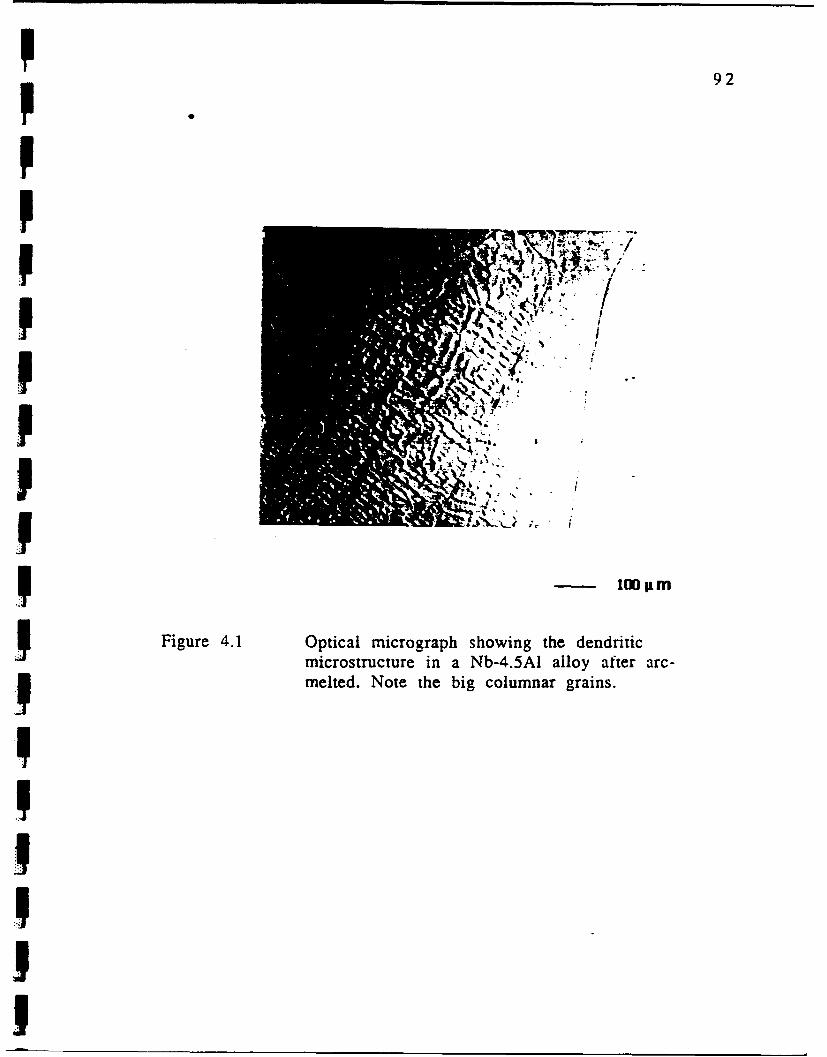
p 92
p
metd Not thebgcluma gan.
.I -- loo zm
SFigure 4.1 Optical micrograph showing the dendritic
microstructure in a Nb-4.5AI alloy after arc-I• melted. Note the big columnar grains.
U
I

p 93
pO
p ~6 U "F B
90 02-*
3 9
9 BB
Bottom Top
0 1000 2000 3000 4000 5000 6000
DistanceS~(Am)
Figure 4.2 A typical experimental composition profile foraluminum obtained by microprobe analysisshowing the microsegregation present in an arc-melted Nb-4.5Al specimen.
I,IJ

I 94
Ii
3 a)
- 10 pm
7-J 6
I€0C
-• <
* 0•
3-
0 10 20 30 40 50 60
Distance
(A m)
Figure 4.3 a) BSE micrograph, and b) a typicalI1 experimental composition profile for Alobtained by microprobe analysis showingmicrosegregation through a dendrite inan arc-melted Nb-4.5A1 specimen.
_I

I 95
gradient in the dendrite, arms in conjunction with the Al diffusion
coefficient reported in Reference [6]. Assuming that the concentration
dependence of Al on distance obeys a simple harmonic behavior [58],
the homogenization time for the arc-melted Nb-4.5at%Al was
1 calculated to be 8.5 hours at 1400 *C.
b. Homogenized Structure
In order to reduce the segregation observed in the as-cast
structure, and therefore reduce the homogenization time, the arc-
melted samples were deformed plastically in compression to a
thickness of about 2 mm from an original thickness of 5 mm. The
mechanical deformation applied broke down the dendritic structure,
making it easier to homogenize the sample. In addition, the specimen
size and shape factors were not a problem, since an adequate
specimen for bonding was easily obtained by trimming the
compressed sample after being annealed.
It should be mentioned that initially, based in the reported Nb-
Al phase diagram [101 a composition of Nb-7at%Al was chosen for
binary diffusion studies. This composition was close to the solubility
limit of Al at low temperatures. After homogenization the
segregation disappeared. However, a precipitate had formed at the
grain boundaries (Figure 4.4). Microprobe analysis showed that this
precipitate has a composition corresponding to Nb3AI (17.3 at%),
whereas the matrix composition was 6.8 at%. In accordance with the
Nb-rich part of the Nb-Al phase diagram (Figure 2.2), at 1400 OC the
solubility of Al in Nb is about 11% and <he second phase must have

96
I IFiue44BEmcor ap f h rleiadan opr
chile qunhe b".A aly-fe
I'
chlld uecedNb7.A 5loyame
homogenization at 1400"C for 2 hours andfurnace c.:oing. Presence of particles Nb 3AI inthe matrix (P3 phase) is observed.
Il

I 97
precipitated during cooling to room temperature Therefore, a lesser
amount of aluminum was added for the preparation of the arc-
melting samples to ensure complete solubility of Al in the 1 -Nb
matrix. The final Al content in alloy P3o used was 4.5 at%.
The plastically deformed samples with an Al content of 4.5 at%
were homogenized at different temperatures and times. When the
temperature and time of the heat treatment exceeded 1400 °C and 8
hours, respectively, extensive precipitation of a second phase in the93-Nb matrix was found. This new precipitate was observed not only
at the grain boundaries, but also inside the grains of the P• phase
(Figure 4.5), and it had a different morphology than that exhibited
by the Nb 3Al. All these characteristics led us to think that the new
second phase could be alumina A120 3. In order to prove this, EDX and
Auger analyses were conducted on a heat treated specimen.
EDX spectra from the matrix and precipitates, both at grain
boundaries and inside grains, were obtained. Results are presented in
Figures 4.6 and 4.7. The higher contents of aluminum and oxygen in
the precipitates in comparison to the matrix content suggest the
presence of aluminum oxide. The larger Nb peak in the spectrum of
the precipitate inside the grain comparing to that at the grain
boundary is probably due to the smaller thickness of the latter in
this instance.
The results from the Auger analysis of these precipitates
confirmed that they are alumina particles. Figure 4.8 shows the
results obtained from a particle which was initially sputtered to
remove the surface layer. The sputtering permitted to achieve a
chemical analysis over a 'fresh' surface approximately 50 A below
98
50ILM
Figure 4.5 BSE micrograph showing the two-phasestructure obtained in a Nb-4.5AI allov afterannealing at 1400"C for 8.5 hrs.

99
a)10 pm
Cursors O.M0keV * 0
I .,
M . .. .. . .I + ii.
0.000 WS 1 024 5.120
b)
Figure 4.6 a) Secondary Electron micrograph, and b) EDXspectrum obtained from the matrix (P3 phase) ofa Nb-4.5A1 alloy after annealing at 14000C for8.5 hours.
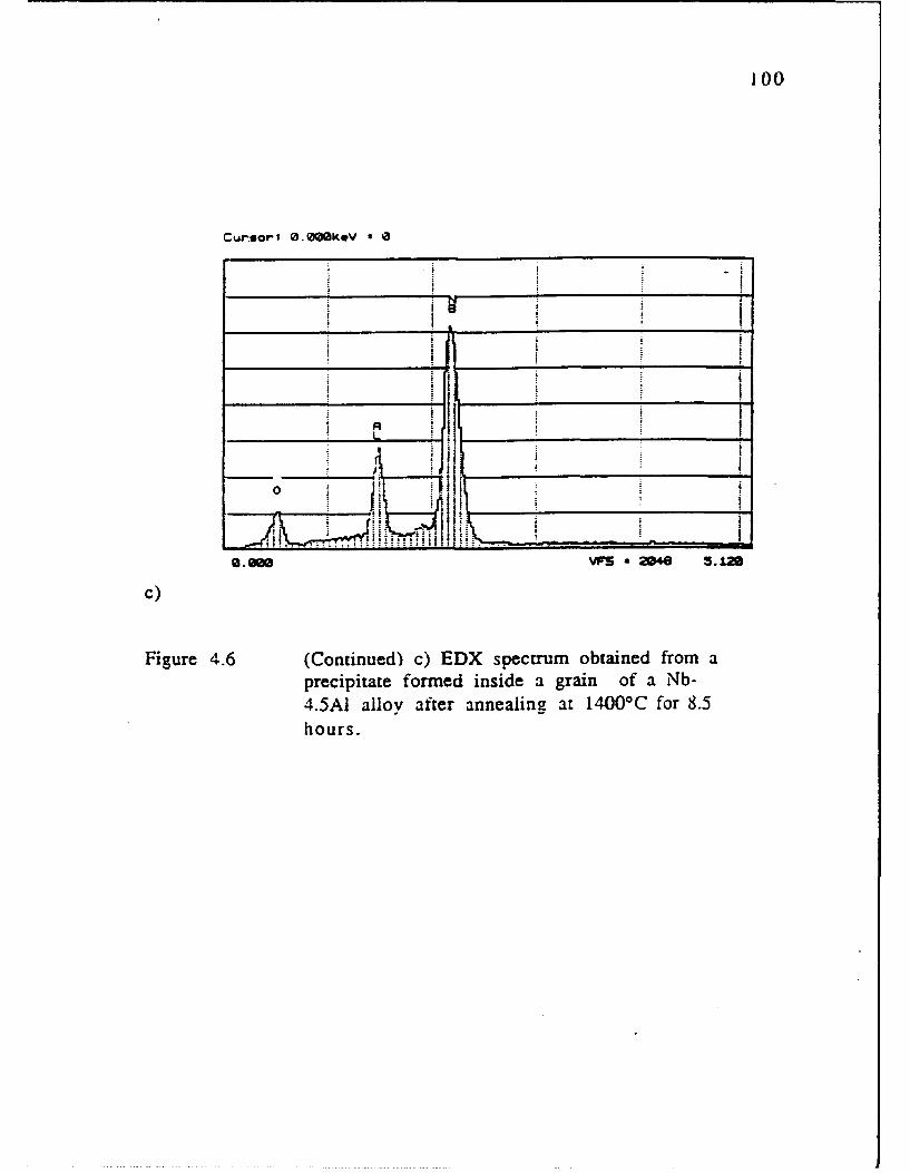
100
Cur~sorI 1. OMKOV
ii
0. Ow*S2D8 3 In
c)
Figure 4.6 (Continued) c) EDX spectrum obtained from aprecipitate formed inside a grain of a iNb-4.5AI alloy after annealing at 14001C for 8.5hours.

101
a)10 I'M
Cu;a-pt'~ O.Oink*V *0
b)~ ~ VF 12 .2
""he i b i
l a i f
__ _ _ " i __ _ __ _ __ _ __ _ _ I
*, [ ."II ' •U !'1_______I>
b) g.e.. ws . eim s.12•
Figure 4.7 a) Secondary Electron micrograph, and b) EDX
spectrum obtained from a precipitate formed atthe grain boundary of a Nb-4.5A1 alloy afterannealing at 1400°C for 8.5 hours.

102
SCALE FACTOR, OFFSEI:443.687, 2357.315 t COIITSSEC W8I.S9tU 81=8.83W8
08 Al
;5"^4w
58.8 258.8 458.8 658.8 891 1981258.8 1450.8 1658.8 185.8 2858.1
Figure 4.8 Auger analysis of a precipitate located inside agrain of Nb-4.5A1 alloy annealed at 1400"C for8.5 hours.
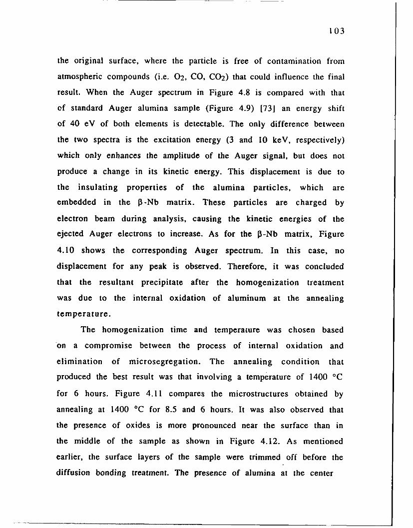
103
the original surface, where the particle is free of contamination from
atmospheric compounds (i.e. 02, CO, CO2 ) that could influence the final
result. When the Auger spectrum in Figure 4.8 is compared with that
of standard Auger alumina sample (Figure 4.9) [73] an energy shift
of 40 eV of both elements is detectable. The only difference between
the two spectra is the excitation energy (3 and 10 keV, respectively)
which only enhances the amplitude of the Auger signal, but does not
produce a change in its kinetic energy. This displacement is due to
the insulating properties of the alumina particles, which are
embedded in the P3-Nb matrix. These particles are charged by
electron beam during analysis, causing the kinetic energies of the
ejected Auger electrons to increase. As for the 13-Nb matrix, Figure
4.10 shows the corresponding Auger spectrum. In this case, no
displacement for any peak is observed. Therefore, it was concluded
that the resultant precipitate after the homogenization treatment
was due to the internal oxidation of aluminum at the annealing
temperature.
The homogenization time and temperature was chosen based
on a compromise between the process of internal oxidation and
elimination of microsegregation. The annealing condition that
produced the best result was that involving a temperature of 1400 0C
for 6 hours. Figure 4.11 compares the microstructures obtained by
annealing at 1400 °C for 8.5 and 6 hours. It was also observed that
the presence of oxides is more pronounced near the surface than in
the middle of the sample as shown in Figure 4.12. As mentioned
earlier, the surface layers of the sample were trimmed off before the
diffusion bonding treatment. The presence of alumina at the center

104
C I
! I€
1.,.
"" • .. . | •,)
S- ] 0
I I i , I I • I-zlU
liB I I I ii I i i i • II i i i i ii i

1 105
oco-
AAD
CD UCS! -S3
I CS!
j C=
I~C Co.o:p
Cbc36 LhA
_Co A
CIDo
c... CID
CC,!
CCo
- 0) 00 r. ~ , ~ ) C~ - CIIUA -C"ccLA
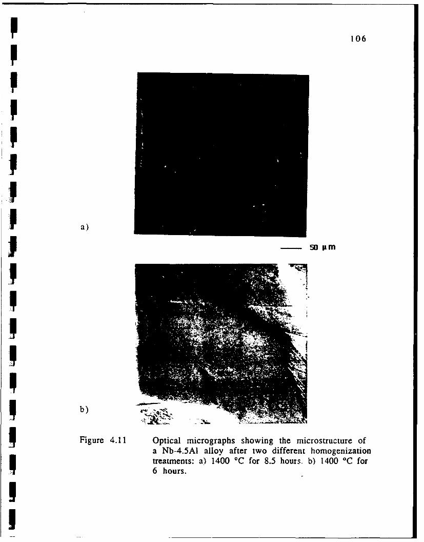
I 106
IaU
I
tramns a) 140_C_ or8._ hus.b)140__ o
6 h orm
I b)
SFigure 4.11 Optical micrographs showing the microstructure of
a Nb-4.5A1 alloy after two different homogenization
treatments: a) 1400 0 C for 8.5 hours. b) 1400 °C for
• 6 hours.U! _________________

5 107
SFigure 4.12 A low magnification BSE micrograph of a Nb-4.5A1 alloy after being heat treated at 14000C
.• for 6 hours. Note how the amount of alumina
precipitation lessen from top (sample surface)Sto bottom (sample middle section.).

P 108
P of specimens was very scarce, with an average separation larger than
100 microns (Figure 4.13). As will be confirmed later, this separation
between alumina particles is much larger than the penetration depth
yielded by the diffusion treatments. Also the aluminum
concentration gradient in the matrix close to the alumina particles
was very small, as illustrated by the microprobe analysis shown in
Figure 4.14. Therefore, even though we could not retard the internal
oxidation of the Nb-Al alloy, the extent of it was reduced
* considerably to such a grade that was considered not to have any
influence on the diffusivity measurements. The grain size achievedI. after the homogenization treatment was very large, approximately9 ASTM 2 size (Figure 4.11).
* c. Diffusion Bonding
After being homogenized and metallographically prepared, theI3-alloy specimen as well as the pure Nb sample were bonded
together in a hot-press furnace. Initially chopped zirconia (ZrO2)
particles of less than 1 gm in size were used as inner markers. Figure
4.15a shows the resultant bonded structure, which looks perfectly
clean, free of any kind of precipitation. After the diffusion treatment,
extensive precipitation of alumina appeared near the interface on the
Nb-Al side as shown in Figure 4.15b. According to thermodynamic
data given in Reference [74], zirconia and alumina have similar free
energy of formation for equal moles of oxygen. Alumina is more
I stable at lower temperatures but ZrO2 becomes more stable at higher
temperatures. According to the results found in this study

P 109
pp
I M
I -|
1 Figure 4.13 BSE micrograph of a Nb-4.5AI sample as-homogenized condition. Alumina presence inthe P-phase matrix is very scarce.I
I.UI.II_ ____

110
a) -
12-
a 10-
0 8
6-
b) 4- 1
0 10 20Distance
0(1m)
Figure 4.14 a) Secondary Electron micrograph, and b) Alcomposition profile of 13-phase matrix close to
San alumina particle.
1

p 111
I
P a)
P - 10 pm
b)
Figure 4.15 A low magnification BSE micrograph of a diffusioncouple with zirconia markers: a) Before diffusiontreatment, and b) after diffusion treatment at 1400*C for 4 hours.
I

112
apparently a reaction between Al and ZrO2 took place, and therefore
the use of zirconia markers was discarded and yttiria Y2 03 markers
were used instead. As in the previous case, a clean, precipitate-free
bond was obtained under the same experimental conditions. Figure
4.16 shows the structure at the interface along with the composition
profile obtained using microprobe analysis. The analytical result
suggests that the boundary is sharp, indicating very limited
diffusivity of aluminum in the Nb side, a highly desirable feature for
the initial bonding of the diffusion couples.
4.2 Diffusivity Analysis
The experimental concentration profile obtained by microprobe
analysis from each of the treated diffusion couples were fitted to a
smooth curve. Determination of the Matano plane position permitted
to compute the interdiffusion flux, concentration gradient and
interdiffusion coefficients at each diffusivity temperature. Under the
assumption that DAI.NNb>>DNb.NAI, the intrinsic diffusivity of Al in Nb
as a function of composition was determined. Then, the temperature
dependency of the coefficient of diffusion of Al in Nb, as well as the
corresponding activation energy and frequency factor values were
calculated.

113
a)10 PM
8-
6
0
0 - 4
E
2- interface
b) 0
0 10 DIstance 20 30
Figure 4.16 a) BSE micrograph of diffusion couple interfacewith Yttria markers before diffusion treatment,and b) the aluminum concentration profileacross the boundary.

114
4.2.1 Postdiffusion MicroStructural Analysis of Binary Diffusion
Couples
The use of yttria particles as markers in the diffusion couples
inhibited the alumina precipitation along the bonded interface after
the diffusion heat treatment. Figure 4.17 shows the resulting
microstructure of a couple after interdiffusion treatment. The alumina
in the structure of alloy P3o was present scarcely not only along the
bonded interface of the couples, but also in the matrix. This fact helps
to explain that zirconia particles were the source of oxygen for
extensive formation of alumina near the bonded interface, but the
material itself also had a propensity to internal oxidation of
aluminum in the alloy. Chemical analysis of the interstitial content of
the alloy 130 after diffusion treatment is reported in Table 4.1,
together with that for the ternary alloys.
4.2.2 Measurement of Concentration Profiles
The microprobe analysis performed used a beam size of
approximately one micron. Therefore, the data for the composition
profile were obtained from points one micron apart. A statistical
resolution (standard deviation) of 0.1 at.% in the counting process was
obtained by employing a beam intensity of 100 nanoamper and a
dwell time of 200 seconds maximum at each point. When either a
lower current or a shorter counting time was employed the tail of the
aluminum concentration profile on the Nb side of the couple was
missed (Figure 4.18). The compositional resolution obtained by the

115
a)
b)
Figure 4.17 Backscattered electron micrographs showingthe resultant microstructures of a Nb/Nb-4.5AIdiffu:ion couple after diffusion treatment.a) Near interface. b) Away from interface.

116
- I -
*
�J3U,
000 �oCu
o Cu
o 0
CU -�.- ,-
U,I-0 --- -
- CuE
0 U,>1
Cu CU-S
Cu
So �- �- �. �- -�
Q
*

117
5
1450 °C. 4.5 hrs
CL
Ea- 2-
00
0 10 20 30
Distance(Wnm)
Figure 4.18 A typical experimental composition profile foraluminum obtained by microprobe analysis of adiffusion couple Nb/Nb-4.5AI after aiinealing at1450 0C for 4.5 hours. Note the sudden drop inthe Al composition profile in the Nb side of thecouple.

118
microprobe analysis is governed by two factors: the background/peak
intensity ratio, and the counting statistics. When a standard deviation
larger than 0.1% is employed, e. g. 0.25%, the counting time for the
analysis is shorter, and the number of events (x-ray counts) detected
will be smaller. Consequently, in regions where the Al composition is
low, the x-ray counts will be insufficient to be taken into account, and
therefore the aluminum concentration at those points will be detected
as zero%. The change to the condition mentioned above permitted to
detect the missing part of the profile as more counts were detected at
longer times. On the other hand, it was observed that employing
longer analysis time results in a severe contamination of the surface
of the sample, as observed in Figure 4.19. However, comparison of the
experimental composition profiles obtained under the two conditions
revealed no differences in the general result. The measurement of the
Al concentration at each point took approximately 6-7 minutes. In
average, to obtain an entire profile took 5 hours. A minimum of two
profiles were measured for each diffusion couple. A typical
composition profile is shown in Figure 4.19.
4.2.3 Concentration Profile Analysis
The experimental raw data consisting of a set of positions along
the diffusion direction and the corresponding concentrations of
aluminum (atomic %) were fitted to a smooth curve using a modified
spline cubic method [8]. To do so, generally, the set of n data points is
divided into intervals separated by knots. These knots set imaginary
regions along the composition profile in accordance to the general

119
I a)
9 0.05 -
0.0 1350 OC. 21 hrs.
3 0.02-
3 0.01Markers Position
0.00 -010 2'0 30
DistanceI b)eerm ta (P~ M)
IFigure 4.19 a) Secondary electron micrograph, and b) atypical exeietlcomposition profile for
Alotie ymcorb nlssoNb/Nb-4.5A1 diffusion couple after annealingI at 1350 *C for 5.5 hours.

I 120
shape of the curve in that region (linear, parabolic, or spline cubic).
The spline cubic zone is also subdivided in intervals separated by
knots and then a cubic spline function fits a different cubic
polynomial to the data in each interval of this zone. For example, the
polynomial for the ith interval will be:
CAI(x) = cil + ci 2 (x-xi) + ci3 (x-xi) 2 + ci4(x-xi) 3 (4.6)3where CAI(x)= Fitted concentration curve in the ith. interval
cij = Cubic coefficients for the ith. interval
xi = position of the it data point
xi = position of the ith knot
The coefficients ci1 and the final knot positions are determined by1 minimizing the least squared error of the fitted curve to the
constraint that the function CAI(x) and its first two derivatives must
5 be continuous at each knot. The number of knots used for the cubic
spline fitting is important. The larger number of knots used tends to
minimize the least square error, i. e., increase the goodness of the fit.
_ In addition, five data points per interval must be set so that a third
degree polynomial is adequately fitted. For the case of the modified
spline cubic routine used in this research, the domain of data of the
diffusion experiments are divided into five different regions, as
shown in Figure 4.20. The central part of the data is fitted by a cubic
spline approximation as mentioned above, and the points deemed to
be outside of the diffusion zone are fitted with horizontal lines whose
ordinates are the end concentrations of the alloys forming the
diffusion couple. The reason for this horizontal line sections is that
cubic spline fits do not easily yield flat sections typical of diffusion
data outside the diffusion zone. Since neither the value of the spline
U

I 121
.c.
CP.I -CIS
L. > -"U CA
4D4, *Je-
Cb 4, *-I

I 122
cubic nor its first derivative may be specified at the edges of the
region fitted with cubic splines, small parabolic sections are used to
smoothly join the cubic spline region with the linear zones. These
parabolic sections are constrained to match ordinates and slopes with
the horizontal line sections and ordinates with the cubic spline curves.
When the limits for the parabolic section were not properly chosen,
the fitted curve exh ,ited small discontinuities that do not belong to
the data (Figure 4.21). To avoid this problem several intervals for the
parabolic limits where tried. This matter is discussed in detail in a
subsequent section.
I The program used for curve fitting produced two output files.
One file contained the polynomial equations employed for the other
subroutines to calculate parameters such as the Matano interface,
interdiffusion fluxes, concentration gradients, and coefficients of
interdiffusion; the other output file contained 100 data points of the
fitted curve, which were also computed by the polynomial equations
in the previous file. Figure 4.22-4.26 contrast the experimental
profiles with those after curve fitting for the different diffusion
treatments performed in this investigation. It can be observed that
there are not discontinuities along the entire profile and a smooth
curve could be obtained.
I 4.2.4 Calculation of the Interdiffusion Coefficient
5 a. Determination of the Matano Interface
J The position (,f the Matano interface was calculated in order to
evaluate the coefficient of interdiffusion in the binary alloy couple

123
I 1400 °C, 8,.5 hrs.0.05
5 discontinuity
c 0.03
7= o
0 0.02
I 0.01-
IC discontinuity
0 10 20 30 40Distance
(A M)
Figure 4.21 A typical composition profile for aluminumafter incorrect spline cubic fitting. Note thediscontinuities along the curve.
I

124
I
Figure 4.22 Fitting of experimental composition profiles by
the spline cubic method for the Nb/Nb-4.5AIcouple heat treated at 1350 'C:a) Experimental curve,b) Fitted profile.
IIIUII
U
|

P 125
I5I 1350 *C. 21 hrs.
I C 3-
o 2-
1Markers Position
0~010 20 30
a) Distance
(p m)
I ~4 _
1350 *C, 21 hrs.
ICc 3-0 E~ S
0a 2-
1 Markers Position
0~0 10 20 30Sb ) Distance
(O m)

126
SFigure 4.23 Fitting of experimental composition profiles bythe spline cubic method for the Nb/Nb-4.5Alcouple heat treated at 1400 *C:a) Experimental curve,b) Fitted profile.
iI
I1

127
0.04-
1400 *C. 8S hrs.
0.03-
C -
0.02-
E0
0.01
Markers Positon
0.00' .1-0 10 20 30
Distancea) (IL m)
0.04-
1400 SC. 8.5 hrs.0.03-
o
0.02-a_ u
oL aE
0.01,
Markers Position
0.00*0 10 20 30
b) Distance(ILm)

128
Figure 4.24 Fitting of experimental composition profiles bythe spline cubic method for the Nb/Nb-4.5A1couple heat treated at 1450 *C:a) Experimental curve,b) Fitted profile.

129
0.05
1450 *.4.5 hru.
0.04-
C - 0.03
o -~0.02-
0.01- 106
Markers Position
0.00-0 10 20 30
Distance
0 .05-
.2R
0 0.01-
0 20 30Distance
b) (ILmr)

130
Figure 4.25 Fitting of experimental composition profiles bythe spline cubic method for the NbfNb-4.5Alcouples heat treated at 1500 °C:a) Experimental curve,b) Fitted profile.

131
0.05
0.04 1500 *C. 5.5 hrs.
0.03-o
CLE •
o m 0.02-0-
0.01
Markers Position
0 .0 01 . I
0 10 20 30 40 50
a) Distance(rn m)
0.05
0.04-
1500 °C. 5.5 hrs.
c 0.03-
E .
o 0 0.02
0.01 -Markers Position
0.00-
0 10 20 30 40 50b) Distance
(PA m)

132
Figure 4.26 Fitting of experimental composition profiles bythe spline cubic method for Nb/Nb-4.5AIcouple heat treated at 1550 °C:a) Experimental curve,b) Fitted profile
Note: Position of the marker plane was notdetermined accurately at 1550 °C; instead,position of the Matano Plane in the fittedprofile is provided.
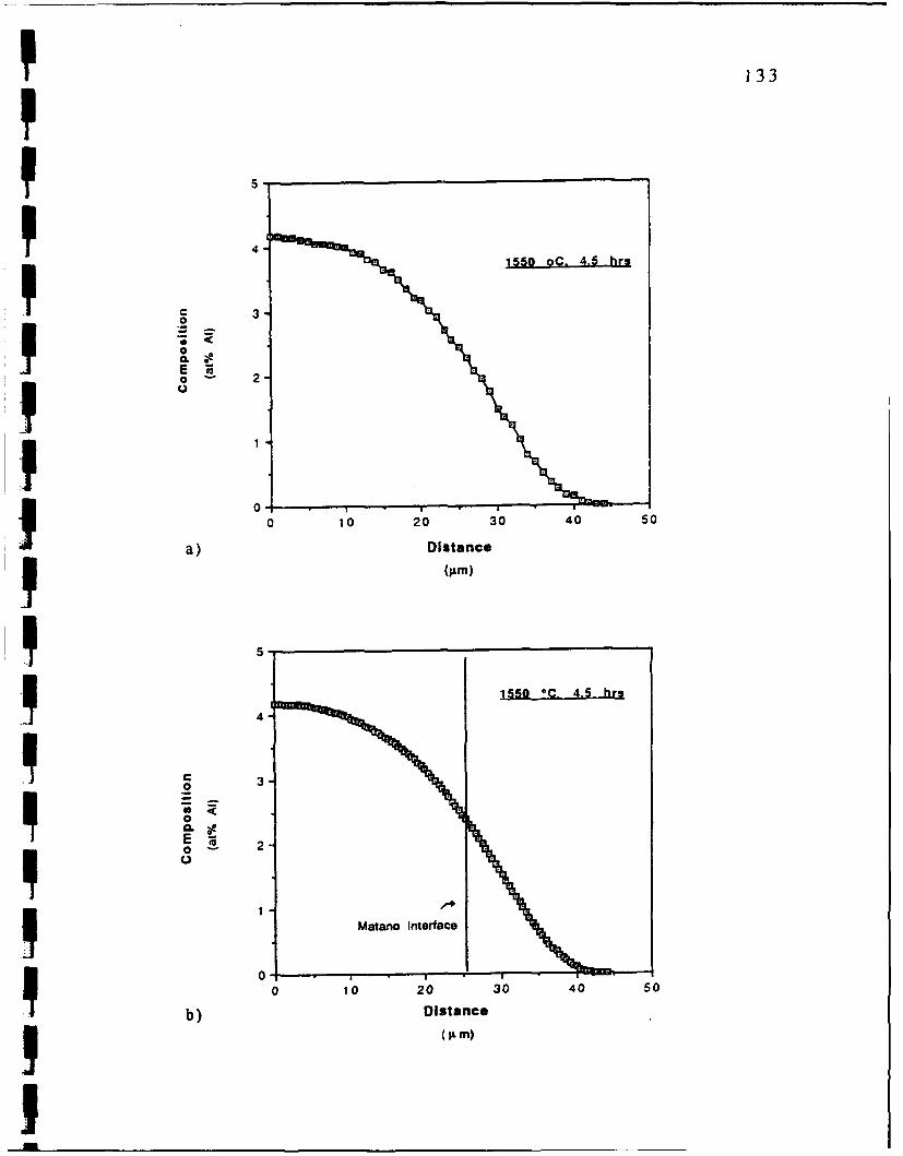
p 133
4_
1550 oC. 4.5 hrs1 3-
00
E a-a 2-
0 10 20 30 40 50
a) Distance
(gm)
!5
I 41550 O C 4.5 hrs
o- 2I 2-Matano Interface
0 10 20 30 40 50
b) Distance
(A M)

I 134
I using the Matano-Boltzmann technique. The position of the Matano
plane can be determined as a function of known quantities as:
Xm = (x- CAI- - X+ CAI+ + (A)) / (CAI- - CAI+) .......... (4.13)
where (A) = entire area under the curve.
x-, x+ = terminal position values at the end of the diffusion zone.
CAI-' CAI+ = terminal composition values at the end of the
diffusion zone.
Equation 4.13 was applied to the fitted composition profiles computed
for Al concentration data from each diffusion couple as those shownin Figures 4.22-4.26.
b. Evaluation of Ju(x)
The interdiffusion flux Ji was calculated as:
Ji(x) =l/2t [ (x - Xm) Ci(x) - ( x+ - Xm) Ci+ + J Cidx ] ...... (4.16)
Here t is the diffusion time and Ci+ is the terminal concentration of
the ith component at the right end of the diffusion zone. Once the
Matano interface is evaluated, all the parameters in equation 4.16 are
known, and the interdiffusion flux can be evaluated at each point on
the concentration fitted curve. Figure 4.27 and 4.28 show examples of
the computed interdiffusion flux profile. As expected, the maximum.I value of flux is obtained at the Matano plane location, and it is larger
at higher temperatures.

1 135
I1350 OC. 21 hrs.
I- 6
I -*En
S~Interface
N0
010 20 30Distance
a) (A M)
SFigure 4.27 a) Typical calculated interdiffusion flux profiles
I for binary diffusion couples Nb/Nb-4.5AIinterdiffused at 1350 *C.
Disanc

p 136
S1550
C. 4.5 hra.
40OI wS 30-
Co - 20
,•U.*0 o
S10 Matano
1 ~. .Interface
0 10 20 30 40 50Distance
b) 0( m)
"I Figure 4.28 b) Typical calculated interdiffusion flux profilesfor binary diffusion couples Nb/Nb-4.5Alinterdiffused at 1550 'C.
II

I 137
U c. Evaluation of Concentration Gradient
UThe composition gradient was calculated by finding the
analytical derivatives of the fitted equations to the concentration
profile. It was found that the calculated concentration gradient was
very sensitive to the choice of the limits for connecting the parabolic
zone to the linear and spline cubic regions during the curve fitting
procedure. Even though the concentration fitted curve appeared to be
smooth and continuous, the fitting method did not provide a
continuous derivative, and discontinuities and/or jumps in both
gradient concentration and diffusivity curves were observed (Figure
4.29). It was noted that the number of knots employed into the cubic
spline region affected such profiles. By try and error suitable limiting
positions of the different regions along with different number of
knots, that resulted in a smooth curve for the concentration gradient
as a function of position, were obtained. It was noted that the linear-
parabolic connection was easier to fit than the parabolic-spline cubic
one. The link of the three regions was easier to get in the pure Nb
side of the couple as the concentration profile was steeper at very low
Al concentrations, where the parabolic region extended for a few
microns. The connection on the other side of the couple, on the other
hand, was much more difficult as a larger penetration of the diffusion
zone in the Nb-Al alloy (P3o) was obtained, producing a less step
concentration gradient. This asymmetry in the concentration profile,
with a deeper penetration on the high aluminum side, reflects a
difference in the intrinsic diffusivity of the two components,
indicating that the aluminum may move faster than niobium.

1 138
Fiue42 T~ypical cacltdcomposition gradientaninterdiffusion coefficient profiles illustrating
I false peaks due to a bad designation ofparabolic regions during the fitting procedurefor binary diffusion couples Nb/Nb-4.5AIinterdiffused at 1550 *C.
a) Derivativeb) Coefficient of Interdiffusion
II
-1Fiue42 yia acltdcmoiingain n
. nedfuincefcen rflsilsrtnfas ek u oabddsgaino
paaoi ein uig h itn rcdr

1 139
10 ___________
1550 °C. 4.5 hrs.
I0N
"tl
.2-10
0 10 20 30 40 50
Distancea) iO m)I
10 _ _ _ _ _ _ _ _ _ _ _
- a
I2
00
0 10 20 30 40 50
Distanceb) I�9 m)

I 140
d. Evaluation of Diffusivity. Activation energy, and Frequency Factor
When adequate links were set, smooth profiles of interdiffusion
coefficient were obtained. Figures 4.30-4.34 present the calculated
composition gradient and composition-dependent interdiffusion
coefficient curves for the b.c.c. solid solution of the binary Nb-Al
system in the temperature range of 1350 °C to 1550 °C. The
interdiffusion coefficients are summarized in Table 4.2, where the
variation of the interdiffusivity with the composition is evident as it
drops at lower Al contents. The interdiffusion coefficient showed a
linear dependency on the Al concentration as shown in Figure 4.35.
The diffusivity coefficient doubles its value at a given temperature
with an increase in concentration from 1 to 3 at% Al. This strong
dependency suggests that the activity coefficient of Al depends
considerably on the composition of Al.
The variation of the interdiffusion coefficient as a function of
temperature was found to obey an Arrhenius type behavior. The
activation energy and frequency factor values were computed
according to:
D= Do exp (-Q/RT) .......... (4.17)
Table 4.3 shows the resultant values of Q and Do as a function of
composition. The average values for the activation energy Q and
frequency factor Do in the temperature range from 13500 to 1550 0C
were found to be:
Q= 80.165 Kcal
Do=0.1136cm 2/sec

141
Figure 4.30 a) Composition gradient, and b) interdiffusioncoefficient profiles for Nb/Nb-4.SAI diffusioncouple heat treated at 1350 0C.

1 142
151 1350 OC, 21 hru.
Tw E
C
a -
0
" E
0
0= 10 20 30
a) Distance
0.3 115 OC 1 r
u s 0. 2 1oi -= I. 1
0 is
C00.1-2 3
0a) Distance 203ILM

143
Figure 4.31 a) Composition gradient, and b) interdiffusioncoefficient profiles for Nb/Nb-4.5AI diffusioncouple heat treated at 1400 "C.

144
10"
1400 *C. 8.5 hr..
0
S S0.I
*-1
C '
-20I
c S -
o E0
-30-
-40-0 10 20 30
Distancea) (a m)
0.4
9-
W 0.3-
C0 1400 *C. 8.S hrs.
*;:00
.2 0.1.
0.00 10 20 30
Distance() IL m)

145
Figure 4.32 a) Composition gradient. and b) interdiffusioncoefficient profiles for Nb/Nb-4.5AI diffusioncouple heat treated at 1450 °C.

146
10'
1450 "C. 4.5 hr..
0.
* -10-
(3
c . 20,
.230
-40.50
0 10 20 30
Distance
a) OL m)
1.0'
14S0 C- 4.5 hr..
0.8
0.4
w
C o-02
0.0
0 10 20 30
b) Distanceb) M)

I 147
I
I
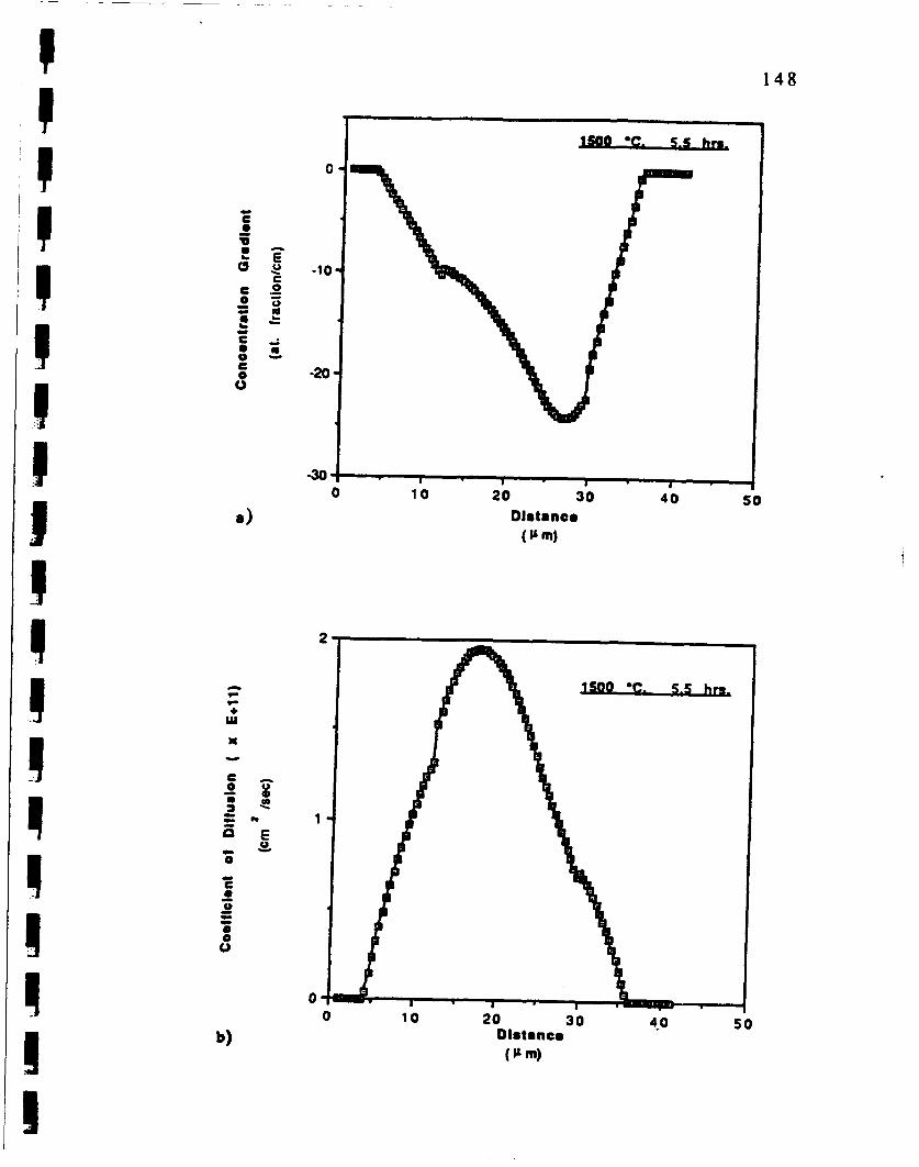
1 148
I1500 "C. 5.5 hrs..
C00
I* -~ E -10.
C
c.2* .w
0 -20
.30-0 10 20 310 40 50
Oa) Distance
(ILm)U* 2
S1So0 oC. 5-5 hr
SEI00
I00 10 20 3'0 4'0 50b) DistanceI (IL M)
I€

I 149.I
I
.11

1 150
50 1550 "C. 4.5 hra
I 0-S -10
-C!I
CE
0 * .h
o -I0-20 4
l0 O 20 30 40 50
a) ODistance
-1550 OC. 4.5 hi's
w 3-
(Am
!2-I 22
10 10 20 30 40 s0
b) DistanceI (it M)

151
I"q -T- -
I~ C 14r
C~
0 0
CaC
I, 00 00 r-
0 C4 -ý
C)
0.0

F 152
F-S
IIUC
0 0
(at% Al)
Figure 4.35 Dependec Of the iflterdiffusi0 n Coefficient 0,thAtcompositOn at several temperatures.

I 153
C
0" 0 r- w
CC
I =0
o ' - 00 00 - C 001~ 0 ..
r- '. - 'o c- A jcc'0 ~ '
> 3 - r ~

I 154
4.2.5 Calculation of Intrinsic Diffusivities
In accordance with Darken's analysis (section 2.2.1.4), equations
2.38 and 2.39 permit to evaluate the intrinsic diffusion coefficients of
binary system when the experimental parameters such as marker
velocity and concentration gradient are known. The results of this
research, however, indicated that the position of the Matano interface
is very close to the markers position; the distance between the final
marker position and the Matano interface for the largest depth of
penetration (1550 1C, 5 hours) was less than a few micrometers,
which is within the accuracy of the measurements. Therefore, the
interface velocity could not be calculated accurately. The intrinsic
diffusivity of Al was estimated (Table 4.4) by assuming that
DAI NNb >> DNb NAI:
D - DAI NNb
SThis assumptions is justified by the fact that the self-diffusion
coefficient of Nb in the temperature range of this study is in the order
of 10-13 cm2/sec. [22, 23]. It is acknowledge that alloying increases
the diffusivity of Nb, however, it is expected to be orders of
magnitude smaller than -10-11 cm2 /sec, which is the interdiffusion
coefficient calculated for the Nb-Al binary system. Furthermore
NAI<<NNb in the couples studied. Figures 4.36 to 4.40 present the
Arrhenius plots for different aluminum concentrations (1% to 3%).
The calculated activation energy and frequency factor values are
given in Table 4.5. The diffusivity data for lower and higher Al
I contents were not considered since large errors are obtained in the
.I

I 155
~ -N1 '0 --N -'rcN
1 -- - -T el
In 00e wl r n
I z,
0C
00 - er4 o0ý
0- Cý 4h 0I ~~~e co ' 0 ,i~-
0 w ri

P 156
p
pp -10.0
i 3 at% Al
Q= 78.7 Kcallmoi.2
Do: 0.1028 cm isee
-10.5
- E
-11.5
y = - 0.98784 - 1.7281x RA2 = 0.952-12.0,,,
5.4 5.6 5.8 6.0 6.2l/T (E+4)
Figure 4.36 The temperature dependency of the intrinsicdiffusion coefficient of Al in Nb at the aluminumconcentration of 3.0 at%.

!157
II -10.0 .
SQ, 81.2 Kcallmole
-10.50Do 0.1795 cm /30SC-10.5
I -11,5 O•'
y120-y0.74599. 1.7821x RA2 = 0.969".12.0-,,
5.4 5.6 5.8 6.0 6.2
lIT (E+4)
(K
Figure 4.37 The temperature dependency of the intrinsicdiffusion coefficient of Al in Nb at the aluminumconcentration of 2.5 at%.
II

I158I
I
I -10* __=__mole
Do= 0.1192 cm 2 !sC
p y . 3 -12 - 0 1 972
5.4 5.6 5.8 6.0 6.2
1/T (E+4)
: ~~(K"' oFigure 4.38 The temperature dependency ofthe intrinsic
diffusion coefficient of Al in Nb at the aluminumII concentration of 2.0 at%.
I- E
I

159
-10-1.5 at% Al
O= 80.4 Kcaumole
Do= 0.1013 cm /sec
01 -11
E
y = - 0.99457 - 1.7665x RA2 = 0.975
-12'5.4 5.6 5.8 6.0 6.2
11T (E+4)
(K)
Figure 4.39 The temperature dependency of the intrinsicdiffusion coefficient of Al in Nb at the aluminumconcentration of 1.5 at%.

160
-10
1. at% Al
Q= 80.1 KcalimoleDo= 0.0776 cm /sec
-12'
y ,, .M03 - 1.7596x r.'12 =0.977
-135.4 5.6 5.6 6.0 6.2
1/T (E+4)
.121
(K)
Figure 4.40 The temperature dependency of the intrinsicdiffusion coefficient of Al in Nb at the aluminumconcentration of 1.0 at%.

161
ppp
L..
0p C's00 � � '.0 -
0% - I- '.0C r- -
- - - -�I 0 - -
- '� C CI _
00, _-
00
00 00 ?-' I,,
0% � C'.'0 - r� �r -
- - - - C
('- 00 00 00 00 00
�ujI
� _I _
UII ____ ____
I<II

P 162
integration step when the composition is close to the terminal
compositions. The linear curve fitting obtained is very good as shown
by the values of the correlation coefficient R2 (>0.95) in the worst
case). The average values of the activation energy and frequency
factor for the diffusivity of Al in Nb in the composition range of 1.0 to
3.0 atomic percent of Al are calculated to be
p Do = 0.1161 cm2/sec,
Q = 80.2 Kcal/mole
i 4.3 Discussion
There has been only one reported study on the diffusivity of Al
in b.c.c. Nb [6]. As detailed in Chapter 2, Bodrov and Nikolaev [6]
calculated the diffusion coefficient of Al in Nb at the temperature
range of 15000 to 1950 'C by an analysis of the kinetics of
evaporation of Al present as a dilute impurity in Nb in a
concentration range of 10-2-10-3 at% using atomic absorption
spectroscopy. In order to compare the results of this study with
theirs, the DAI values were plotted as a function of Al concentration.
The DAI values for dilute solutions were estimated by the
extrapolation of the Al intrinsic diffusivity to zero concentration. With
the extrapolated results a new Arrhe•ius curve was obtained which is
shown in Figure 4.41 together with their results. The DA! values
calculated in this study are an order of magnitude smaller.
Furthermore the activation energy reported by Bodrov and Nikolaev
I

163
p
0 (Iccal/mole)
0 102 a Ref.161
-9- 74.3 0This wor
I"10
E -11
-12
1 -13-4.5 5.0 5.5 6.0 6.5
l/T (E÷4)I (K
Figure 4.41 Comparison between this work and Ref. [61 for thetemperature dependence of the diffusion coefficientof Al in Nb.
1lII

P I164
[61 is much larger (102 Kcal/mole) than the value obtained in this
study (74.3 kcal/mole). These discrepancies can be discussed in terms
of the differences between the two studies:
(i) Method: The indirect method of evaporation of Al employed
by Bodrov and Nikolaev involves assumptions, which their validity is
not justified (see section 2.1.2). The traditional method employed in
this sudy is a direct method and is believed to yield more accurate
results.
(ii) Temperature range: This study was conducted a lower
temperature range 1350-1550 °C in comparison to 1500-2000"C,
which was applied to their experiments. The self-diffusivity of Nb is
reported to be very high close to its melting point [23]. This
phenomenon has been attributed to the rapid motion of divacancies
at high temperatures [52]. This section was explained in detail in
section 2.1.2. The contrioution of divacancies at high temperatures
can explain a larger activation energy and higher diffusion coefficient
. at temperatures close to the solidus temperature of the alloy.
However, since there is an overlap of test temperature between this
study and that of Bodrov and Nikolaev the low diffusivity of Al
measured in this study can not be explained solely by a divacancy
mechanism.
(iii) Interstitial Content: The processes of bonding anid diffusion
treatment introduced a high concentration of nitrogen and oxygen in
the alloys used in this study (see Table 4.1). Eizinger et. al. [23] have
reported that oxygen content has no effect on the self-diffusion of Nb.
Al is expected to bind with oxygen, however, such trapping would
expect to increase the activation energy in comparison to a purer

I 165
system. Therefore, the observed inconsistency can not be attributed
to the relatively high concentration of interstitials in the alloys used
in this study.
Bodrov and Nikolaev also measured the intrinsic diffusivity of
Al in Ta:
Do= 1.525 cm 2/sec
Q= 73.14 kcal/mol
D 15000=1.3646 x 10⁻⁹ cm 2 /sec
It is interesting to note that the Q value for Ta-Al is much smaller and
closer to the Q value found in this study for the Nb-Al system.
Furthermore a recent work by Maslov et. al. [75], who have
9 investigated the diffusion of Al in V in the temperature range of
1000-1500 OC, gives:
9 Do= 0.084 cm 2/sec
Q= 64.1 kcal/mole
The activation energies for self-diffusion of Ta, Nb and V normalized
for melting point (Q/Tm) are very close [28, 76] (see Figure 2.10), and
the phase diagram of these elements with Al are very similar.
Therefore one would expect that the activation energy for diffusivity
of Al in Nb to be in between that in Ta and V, consistent with the
result obtained in this study.
Most of the existing interdiffusion studies including Nb as one of
the components are those involving another transition metal as the
Ssecond component in the diffusion couple. Table 4.6 [77] present the
value of the activation energy for the binary system Nb-X (X= Ti, V,
Zr, Mo, Ta, W, Al). In this Table the intrinsic diffusivities of the solutes
J are compared to the self-diffusion of Nb. All these elements form
!

p 166
Oo n'
z4NO~
2NCU 0 0i- >0

U 167
extensive b.c.c. solid solution regions in the phase diagram when
combined with Nb. Except for Mo and W, the other elements show
relatively a similar activation energy for diffusion. Although Al is not
a transition metal, the results of the ternary diffusivity obtained in
this study (see Chapter 5) suggest that in the Nb corner of the ternary
phase diagram Al and Ti have similar penetration tendencies at 1200
3 °C and 1400 'C annealing temperatures. Again, this observation
suggests that in comparison to the Bodrov and Nikolaev study the3 lower diffusivity coefficients obtained in this study correlate better
with the diffusivity of Ti in Nb.
The results of interdiffusivity for different phases in the Nb-AI
3 system are summarized in Table 4.7 [78-80]. The activation energy
for the interdiffusion in the [3 phase is somewhat smaller than Nb3AL.
3 The activation energy seems to decrease with increasing the Al
content and for NbAI3 it reaches the activation energy for self-
diffusion in pure Al (35 kcal/mole) [771.
4.4 Summary
The binary diffusion in the 1 Nb-AI solid solution was
evaluated by the Matano-Boltzmann method. The Nb-4.5AI alloy
5v used for this research was susceptible to internal oxidation. The
formation of A1203 near the interface could be lessened substantially
3 by using yttria markers instead of zirconia ones. Due to the oxidation
restriction both temperature and time of interdiffusion treatment
had to be shortened and therefore, the extent of composition profiles
3 obtained was limited to a maximum of 45 gim. As a result,
I

I 168
4 ) >
c
a Ci
ccI.
~d -

I 169
"U appreciable movement of markers after interdiffusivity was not
detected either.
Spline cubic fitting of the experimental composition profiles
vicrked successfully, even though difficulties arose during curve
fitting, specially in the parabolic region of the profile in the 1Po alloy
I side of the diffusion couple.
The results of this study indicate that the interdiffusion
coefficient in P3 solid solution of Nb-Al system varies linearly with Al
composition in the concentration range of 1-3 at% Al and it follows a
linear Arrhenius behavior as function of temperature in the 1350 'C-
1500 *C range. The activation energy for diffusivity of Al in Nb was
found to be 80.2 kcal/mole, wich is smaller than the previously
reported value of 102 kcal/mole that has been obtained in the 1500
*C-1900 0C temperature range. It is suggested that this discrepancy is
associated with the differences in the evaluation method and
possibly the temperature range.

CHAPTER 5DIFFUSIVITY ANALYSIS
IN THE TERNARY Nb-Ti-Al SYSTEM
The purpose of this part of the study was to investigate the
diffusivity in B.C.C. solid solution of ternary Nb-Ti Al system. The
ternary diffusion couples prepared in this study are illustrated in
Figure 5.1.
The Nb-42.5at%Ti-15at%Al (01) alloy was chosen as the main
alloy and it was coupled with pure Ti, pure Nb and the Nb-50at%Ti
([3) alloy. The composition of Al was chosen based on the information
available on the 13-transus temperature. An increase in the A] content
in this part of the ternary phase diagram results in an increase in the
S[3-transus temperature and order-disorder temp,-.ratures [811.
Therefore 15 at% was estimated to be the maximum Al content of an
alloy that would have a P3-transus and order-disorder temperatures
below 1000 *C. Two additional couples consisting of the Nb-
47.5at%Ti-5at%Al (132) alloy coupled with the 033 and 13o alloys were
also prepared to complement the binary diffusivity results.
In this chapter the results of the diffusivity experiments
performed on the ternary Nb-Al-Ti system and their discussion are
presented. The first part of the chapter deals with the
microstructural details of the ternary couples before and after the
diffusion treatment. Then, in order to have a better understanding of
5 170

3 171
I
I U
* 0.•
10
* •- ooK3
!C!0

5 172
the diffusivity behavior of the system, the composition profiles
5obtained by microprobe analysis are given in different groups
depending on -the compositional characteristic of the couple. The
information provided by these composition profiles is presented and
analyzed with the help of concepts such as Penetration Tendencies,
Composition Paths, Kirkendall Shifts, and Crossover Displacements. A
summary of the findings is given at the end of the chapter.
5.1 Microstructural Analysis
The microstructure of the individual alloys and the diffusion
couples after both the bonding and the diffusion treatments were
investigated using optical and electron microscopy techniques.
Pure Ti undergoes an allotropical transformation at 882 0C,
from a high temperature body-centered cubic (1) phase to a
I hexagonal close-packed (a) structure (see Figures 2.1 and 2.3). The Ti
alloy phase diagrams in the Ti-rich section are usually classified into
three types. Elements that stabilize a-phase and increase the a/P
transus. Aluminum and oxygen are the most important a stabilizers.
Elements that depress the a/03 transus and stabilize P-phase are
classified in two groups: those which form binary systems of the 03-
isomorphous type, such as Nb (see Figure 2.1) and those which
favour formation of a O3-eutectoid such as hydrogen. In general the
microstructure observed is sensitive to the cooling rate from the 13-
phase regime. A fast cooling rate can result in formation of
martensitic ac' phase.

I 173
The as-received Ti used in this study had a duplex
microstructure consisting of a + 10 phases as shown in Figure 5.2. The
small amounts of impurities (see Table 3.1) are sufficient to result in
I an (a + 0) microstructure rather than a single a-phase at room
temperature. On the other hand P3I(Nb-42.5Ti-15AI), 132 (Nb-47.5Ti-
5AI) and 133 (Nb-50Ti) alloys displayed a single phase microstructure
as shown in Figure 5.3, while the phase diagram suggests that these
alloys should consist of a and 13 phases at room temperature. This
observation can be explained by the low mobility of Nb at the a/13
transition temperature for these alloys. TEM analysis of a 50Nb-
40Ti-10AI alloy [821 has revealed that this alloy is composed of the
disorder 13-phase. Although the exact j3-transus temperature for
these alloys are not known, based on the binary Nb-Ti phase
I diagram, they can be estimated to be below 1000 'C.
As shown in Figure 5.4 the duplex microstructure of the pure
Ti persisted after bonding with the 13P alloy at a bonding temperature
of 700 *C, which is below the 13-transus temperature of titanium.
However, in the vicinity of the interface, where some interdiffusion
had occurred, the microstructure consists of a single phase as shown
in Figure 5.5a. The microprobe analysis showed slight penetration of
both Al and Nb to the single phase region as given in Figure 5.5b.
Since Al is a strong a-stabilizer it may be speculated that this narrow
zone of penetration consists of a-phase. Figure 5.5 also shows that a
thin darker band has developed in the ternary side of the couple.
This is probably due to the slight interdiffusion of Ti into the 131
phase which is detected by the composition dependent BSE image. A

I174I
IIIIII
a)I10 iPm1
IIII
b)
Figure 5.2 Micrographs showing the duplex structure(at+f) of the as-received Ti: a) Opticalmicrograph, as-etched condition; b) BSEimage.

I 175
I I0m
SFigure 5.3 BSE micrograph of PI1 alloy (Nb-42.5Ti-15AI) after
S~homogenization at 1400 'C for 6 hours.
I

176
pjpa
I0JI
•i ,-m ,• ~a- ,io.m
Figure 55.4 Optical micrograph of the bonded interface
in diffusion couple #12 (Pl1/Ti) after bonding
at 700 0C for 2 hours showing the duplex
structure cc+p of the Ti side of thecouple.
Ii

3 177
I12o
I ~~~~100- ••-;8TA
- 80
0"7b Al- 0080
220
00
40 Markers Plane •
b, 8 10 12 14 16 18 20Distance
(,.A m)
Figure 5.5 a) BSE micrograph of interface in diffusion
couple #12 (lI/Ti) before diffusion treatment;
b) the three composition profiles across theboundary
I2

I 178
diffusion treatment at 1200 'C resulted in a two-phase region
adjacent to the interfact (Figure 5.6). The microstucture resembles
the typical Widmanstatten (x + J0) structure that developes in Ti
Il alloys. The development of a two-phase region adjacent to the
interface in the 1200 'C treated couple can be attributed to the facts
that (i) at 1200 °C the microstructure consists of single 03 phase, (ii)
the higher temperature allows the diffusion of Nb into the Ti side,
and (iii) the cooling rate achieved in the vacuum furnace is faster
II than that obtained in the hot press, which was used for the bonding
treatment. The acicular morphology of this two-phase region in
comparison to the equiaxed morphology of Ti can be explained by
3 the higher alloying content of it.
Similarly the other ternary couples that were bonded at 900 *C
showed the formation of alpha phase, which precipitated along grain
boundaries and at the bonded interface as shown in Figure 5.7. These
areas have a higher surface energy, which induced the formation of ac
phase. Figure 5.8 shows BSE micrographs where this precipitate looks
dark indicating its high Al content. The effect of the aluminum
3 content on the presence of this second phase is corroborated by the
following observation. No precipitation was observed in the binary
Ti-Nb side of any couple (#7, #9). However, when a small amount of
Al (0.5 at%) was present in the Nb-Ti side (P33) of couple # 10,
precipitation was observed on both sides of the couple as shown in
Figure 5.9. After interdiffusion treatment at either 1200' or 1400 'C,
no a phase was detected anywhere (Figure 5.10), which means that
due to the higher temperature the structure transformed completely
to 13 phase and because of the redistribution of Al and Nb around the
I

p 179
I
I Figure 5.6 Optical micrograph of the Ti side next to thebonded interface in diffusion couple #12(01l/Ti) after diffusion treatment at 1200 'Cfor 6 hours. Note the duplex (ox+Pf) zone withthe acicular morphology next to the interface.
Ii
I=

180
0 Po
F 5 O c mi sw precipitationI of c phase
at t -" an bof
tny Ia bd i
Figure 5.7 Optical micrograph showing precipitation of a phase
at the interface and grain boundaries of the
ternary 131 (Nb-42.5Ti-15AI) side of the couple
after bonding at 900 °C for 2 hours.
IIII

P 181
P10 PmI
b)
SFigure 5.8 BSE micrographs showing precipitation ofox phase in the ternary side of the couplesalong the interface: a) diffusion couple #9
(101/133); and b) diffusion couple #11 (132/100).
I

9 182I
II p
SFigure 5.9 BSE micrograph of bonded interface In
diffusion couple #10 (132113) after bonding at900 °C for 2 hours showing the presence ofi, second phase (oa)on both sides of the interface.
I

183
-'I ,
Fig ure_.1 .roi af
c #6 "ea
i Figure5.10oBSEminatonrp ove the interfceip i ffusion-fe.i structure is detailed.
II

I 184
5 interface and the relatively faster cooling rate, in the vacuum
furnace the precipitation of a phase from 13 was inhibited. After the
diffusion treatment, the couples were reheated at 920 'C in the
vacuum furnace in order to study the stability of the microstructure.
Again precipitation occurred at the grain boundaries, interfaces, and
on the dislocations substructure, but there was a denuded zone near
the interface (Figure 5.11), which matched the diffusion zone after
the heat treatment at 1200 0C. These observations, in addition to the
fact that the structure of ternary alloys after homogenization at 1400
OC consists of the single 13 phase, lead to the conclusion that at the
interdiffusion temperature of 1200 0 C and above the microstructure
was composed of single b.c.c. 13 solid solution.
q 5.2 Composition Profiles
The composition profiles for the different ternary diffusion
couples after interdiffusion at 12000 and 1400 0C for 6 hours, as
obtained by microprobe analysis are shown in Figures 5.12 to 5.18.
Note that the profiles are presented in different scales. At least two
composition profiles were obtained for each couple, as it has been
discussed in Appendix A. Next, the composition profiles for two
different cases are discussed, and the presence of critical points and
the effect of temperature are presented.
I
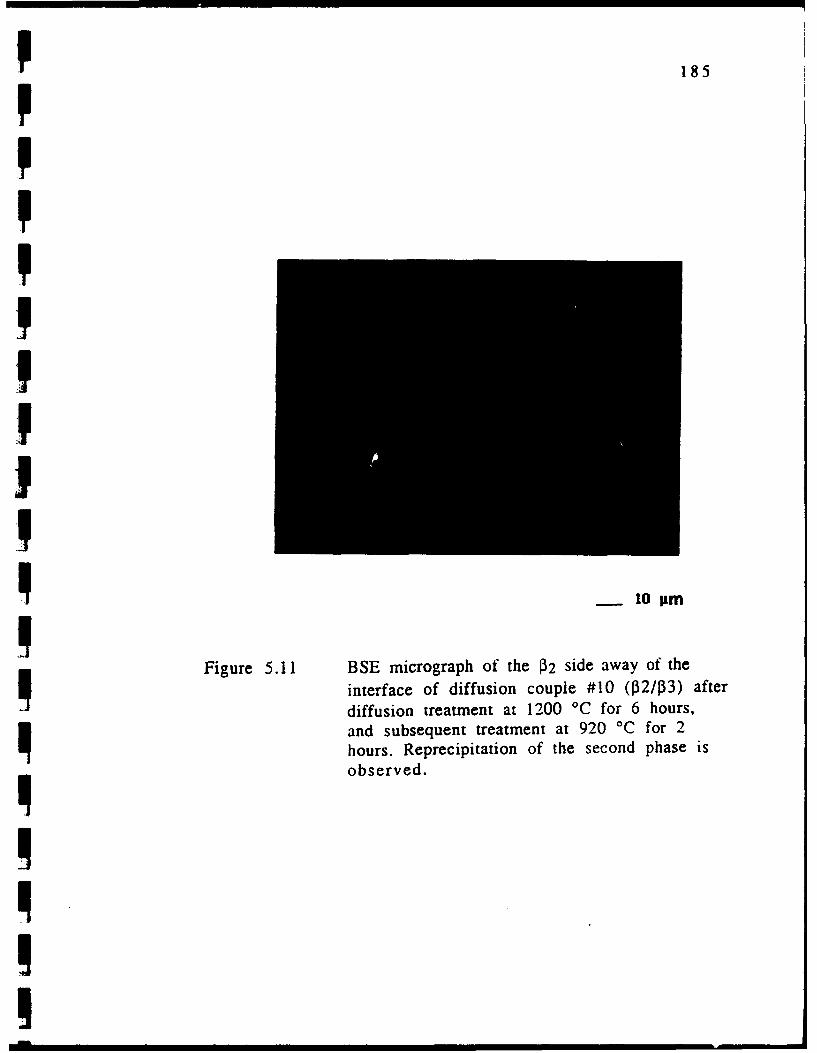
1 185pp
,IUII
I • 10 11m
Figure 5.11 BSE micrograph of the 1P2 side away of the
interface of diffusion couple #10 (132/p33) afterdiffusion treatment at 1200 'C for 6 hours,and subsequent treatment at 920 'C for 2hours. Reprecipitation of the second phase isoI
obered
I

p186
F 100 --0Nb
80
E - Markers 4 t0 40------ - 42 at°/6S~Plans
20-00
-:• ... ... .. .... ... 15.1 at%
250 350 450Distance
(9 m)
Figure 5.12 Penetration curves of the 3 components in the
couple #6 (11/Nb), heat treated at 1400 °C for 6hours.
III
I

p 187
I ~ ~~~~~~60 _ _ _ _ __ _ _ _ _ _ _
50 -
4 ---------- 43.0 at%1 = 40-0
0• 30-
30 Markers Plane - Ti
0 NbI (320-
16.8 at%
10
100 200 300 400 500 600
Distance
(1• m)
Figure 5.13 Penetration curves of the 3 components in thecouple #7 (31/33), heat treated at 1400 IC for 6hours.
III
iI -

188
i 100
8O Nb 131
0 60-
E 4 Markers Plane ------------- ------- 42.5 a[%o 40
20 Al
S T, 16.1 at%S; ~Nb
0 _ ___
250 300 350Distance
(A M)IFigure 5.14 Penetration curves of the 3 components in the
couple #8 (131/Nb) heat treated at 1200 'C for 6hours.
I,IIIr

189p
P ~ ~ ~ ~~60________ _
P 50
S40 ---- ---_ -- 40.2 at%
04.0 . ... .. .. l- i
03 T9 2 Markers - i
0o Plane20 P a - - - - ------ -16.8 at%
10-
200 300 400 500Distance
Figure 5.15 Penetration curves of the 3 components in the
couple #9 (131/133), heat treated at 1200 'C for 6hours.I
iIIiI

F 190
-- NI50250 27 3 5 -- 47.5 at%
40-
.0 Markers-
30D Plane
E # A l
I . .. I )I
20-T
10-
22527323745I Distance
(LM )
Figure 5.16 Penetration curves of the 3 components in the
couple #10 (P2/103), heat treated at 1200 'C for 6
hours.

1p 191
I ~100*
80-
0 60
. 2 o
-a-- Al0 --------- 48.0 at%
o 40 --- Nb
S20- Markers Plane
3.9 at% 4.1 at%0. ----------'
225 275 325 375Distance
(I9 m)
Figure 5.17 Penetration curves of the 3 components in thecouple #11 (2/130), heat treated at 1200 'C for 6hours.
I1
I4
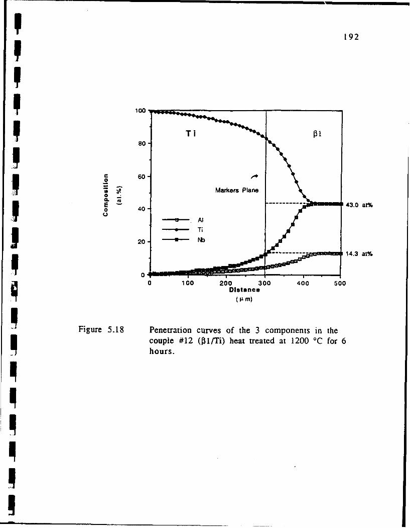
192
1 100
S80, Ti f •8
0 ~60-
Markers Plane
E 40 43.0 atV0 40-
S- AlI • Ti
20 ;.
i • 14.3 at%/
0 1 ;0 200 300 400 500
Distance
(L M)
U Figure 5.18 Penetration curves of the 3 components in thecouple #12 (jDl/Ti) heat treated at 1200 'C for 6
hours.Il
IIJ

1 193
5.2.1 The 01/X couples: Effect of Ti contentIThe penetration curves of the three couples containing 013 alloy
are compared for individual elements in Figures 5.19 to 5.21. It is
observed that the depth of penetration in the counterpart side of 01I• is in general larger as its Ti content increases. For example,
penetration curve for couple #8 shows only a shallow penetration of
the three elements (less than 5 gm) into the Nb side, whereas couples
#9 and #12 show much deeper penetration into the J33 and Ti,
respectively. As to the penetration in the ternary alloy side P31, the
depth of penetration for each element is also larger as the Ti content
of the counterpart side increases.
5.2.2 Effect of Concentration Gradient
Figures 5.22 to 5.24 compare the composition profiles of each
element for two cases with a constant Nb:Ti ratio and different Al
composition gradient (couples #9 and #10). As expected, larger
composition gradient results in a larger penetration depth of Al.
When the Al concentration on both sides of the couple is the same
the composition profile is given in Figure 5.25. A larger diffusion
zone on the ternary side of the couple than that of the binary Nb-
4.5A1 side is observed. However, when the concentration profiles for
diffusion couples #11 (00/032) and #10 (03/P32) are compared to each
other some interesting observations are made (see Figures 5.26-
5.28). It is observed that although the concentration gradients of TiI• and Nb are smaller in couple #10, it has a larger diffusion zone than

194
5 ~ ~~~~~20' _ _ _ _ _ _ _ _ _ _
5 16.8 at%- 16.1 at%
9 Markers Plane 14.3 at%
0
o C L--- #12
0- #9:. -" #8!o
TI0 100 200 300 400 500 600
5 Distance
(11 m)
I Figure 5.19 Penetration curves of Al in three differentdiffusion couples heat treated at 1200 'C for 6hours.
IIII--
I&

195
I ~100'
Nb 1
80
C 60-0 _3 = •,I]3 -- 12
07; Z 50.8 -------- --- -- - -
E-) (3 43.0 at%
3 20 Markers Plane
1 0 100 200 300 400 500
Distance
(p M)IFigure 5.20 Penetration curves of Nb in three different
diffusion couples heat treated at 1200 'C for 6hours.
I
IIUI

196
7IIT1 100 ... i
5 80
O .- Markers Plane
109.1O.L ..... 43.0 at%/
a 40 ...------- 40.2 at%/oU
-0 3- #12120 "----'-'- #8
S~Nb #
0 100 200 300 400 500 600Distance
(11 m)
U Figure 5.21 Penetration curves of Ti in three differentdiffusion couples heat treated at 1200 °C for 6hours.
IIIIU
I l

197
I ~ ~~~~~20 ____________
P3 ------------ ------. ... --- 16.8 at'*/
Markers4
C.,
0 istance 4
(M.m)
I ad#0atrhatramnat20°CorFigure 5.22 Composition profiles of Al in diffusion couples #9
hours.I0I
2;I ' itac ; 0(AM
Fiue52Iopsto rfls fA ndfuinculs#anI1 fe etteteta 20O o
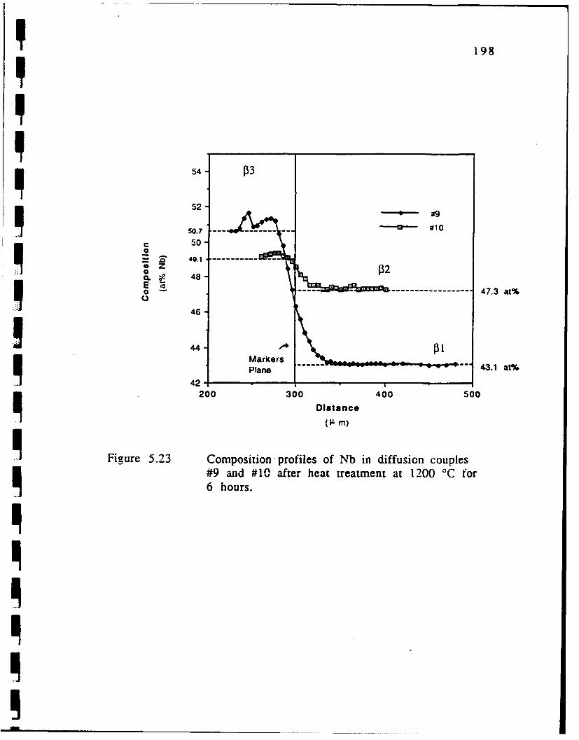
198
I 54 3
52150.7 #10
500
= l 49.1--- - - - - - -
48
Distanc
----------------------------- 47.3 at%.1. (346-
.•Figure 5.23 Copstonpoiesoabindfuio ope
#9 land 1 fer h1a trametat%0 °
6 hours.
I
I420 300____So

1991
1 54. ......
52
5 0 .4 . ... . . . . . .- - - - -1 50
00
.2 . 481 . ........ 47.S at%
I 4 #10
42-
Markers Plane 4 . a
40-40.1 at%
200 300 400 500
Distance
I Figure 5.24 Composition profiles of Ti in diffusion couples #9
and #10 after heat treatment at 1200 0C for 6hours.
III

I 200i6050.71 3PI 6~~~~~0 _____ _-_____-__
I 50.49.3493s .. . S_ -_ _ ._-.. 43 at%
- -1 ---- -------. .. .. . . . . 4 0 .2 a t%
0_G Al
0 30- Ti
E Markers N lb
20 Pl n -- -- -- -- - --..-.-- - 16.8 atQ',,
0
200 300 400 500
Distance
Figure 5.25 Composition profiles of the 3 components at
constant Al concentration (couple #9 131/133))
after heat treatment at 1200 °C for 6 hours.
I

I 201
I87 P2
6
C 50 14.7 at%,;c __0 -- . - . . - -- ---.................. 4.2 at%
CL 39
0102-
Distance 35
I Figure 5.26 Comparison of penetration depth of Al in couples
involving alloy P2 (#10 (1P3/02) and #11 (1303/2))iII

I 202
110096.1 - - - - -
00
"0 Z 70
0 -e- #10
60-
P3350 --- ---.. . ...... 48.0 at%
49.1 47.3 at%
i 40 / 15
250 350Distance
(OL M)
I Figure 5.27 Comparison of penetration depth of Nb in
couples involving alloy 032 (#10 (033/32) and#11 (00/532))
I i II

I 203
50 ------- 48.0 at%47.8 at%
40-
0 30-
20 --- 1
-I10
250 1 tn 350
Distance
S(A M)
5Figure 5.28 Comparison of penetration depth of Ti in couples5I involving alloy 132 (#10 (03/132) and #11 (30/12))
III

I 204
the couple #11 does. This could be explained readily by comparing
the solidus temperatures of the alloys involved in the respective
couples; the 030 alloy has a much higher solidus temperature than the
033 alloy does.
5.2.3 Critical Points
I Except in a few cases, all composition profiles of the couples
studied did not exhibit critical points and their shape was smooth
and similar to that obtained in the binary diffusion studies. Figures
I 5.29 to 5.31 shows the compcsition profiles for those cases, in whichInaxima and minima where observed. An interesting observation is
that these critical points appeared always when the concentration
gradient of the element was small, i. e. for Al in couple #11 (Figure
5.29), for Nb in couples #7, #9, and #10 (Figure 5.30), and for Ti in
couple #9 (5.31). When the diffusion temperature is increased for the
couple 133/131 from 1200 °C (#9) to 1400 "C (#7) the maxima in the
composition profiles of the Ti is completely removed, and for the Nb
at 1400 °C the profile shows a small tendency for maximum. These
observations suggest that limited physical movement of atoms due to
a low interdiffusion temperature, low concentration gradient or high
melting point of the element such as Nb results in the occurrence of
maxima and minima in the concentration curves as obtained by
microprobe analysis. As suggested by DeHoff et. al. [69] the apparent
diffusion zone measured by the microprobe analysis does not
represent the actual physical distance over which the atoms have
moved. When the movement of one element is limited due to the
S

p 205
p8p
* 6
0... <5 Markers Plane0
- 4.2 at*I 3.g
3-
240 260 280 300 320 340 360
Distance
(9m)
Figure 5.29 Critical point observed in the Al composition
profile after diffusion treatment of couple #11(00/4i2) at 1200 °C for 6 hours.
!

I 206
52.
41.1
48.1
48.0
-------- 47.3 at%a e 46
• - #7 wb- •-&-- 43.1 at%
S42 - 41.5 at%
40-100 200 300 400 50
DistanceI (I M)
I Figure 5.30 Critical point observed in the Nb compositionprofile after diffusion treatment of couples #7(130/132), #9 (133/131) and #10 (133/132) at 1200 TCfor 6 hours.
II,I

U207
* ~~~~~~50__ _ _ __ _ _ _ _ _ _
49.3 ------------
48
C 460a- - I-,
0 44-•
42-
.40. 40.1 at%
200 300 400 500
Distance
(A m)
Figure 5.31 Critical point observed in the Ti compositionprofile after diffusion treatment of couple #9133/131 at 1200 *C for 6 hours.
IIIII

208
1 above mentioned reasons, such as Nb in the Nb-Ti-Al system the
atomic fraction profile of this element represent the unequal
mobility of the other constituent elements.
5.2.4 Temperature Effect
The composition profiles for each element of the systems
consisting of Nb/j31/Nb (#6, #8), and I03/131I133 (#7, #9) interdiffused
Nj at 1400 'C and 1200 *C are compared in Figures 5.32 to 5.34 for the
former case and Figure 5.35 to 5.37 for the latter one. At 1400 °C the
general behavior observed in the diffusion couples treated at 1200 *C
is maintained. That is, the penetration depth is larger in the ternary
side of the couples. As expected, the depth of penetration of each
component becomes deeper as the temperature is raised.
5.3 Penetration Depth
As was shown in Figures 5.12 to 5.18 the depth of the
penetration of the composition profiles is not symmetrical in both
sides of a given couple. Table 5.1 shows the depth of penetration for
the different couples as measured by microprobe analysis. Next, each
Ij case is analyzed individually.
a) Df..LNb (1200 'C):In this case the three components show an equal
IN] penetration depth on each side of the couple; however, their
penetration curves are not symmetrical. A much larger penetration is
Nj observed on the J3 side, i. e. the side with the lower solidus
temperature.
Ii

209
I
Nb
- • 16.1 at%
---------------- --------- 15.1 at%
CL
S-e- 1200 °C. #8
9- 1400 °C. #6
Markers Plane
250 350 450Distance
(A. m)
Figure 5.32 Composition profile for Al after interdiffusion
treatment at 1200 °C (#8) and 1400 °C (#6) forfor 6 hours.II
I!I

1 210
p
P 100I
S90 Nb Markers Plano
80O
z 70CL 1400 *C. 96
ao 1200 °C. #860
-- -------- 43.0 at%--- --- --- -- --- --- -- --- --- -- ------ --
40 __42.8 ae%250 350 450
Distance
(A m)
I Figure 5.33 Composition profile for Nb after interdiffusion
treatment at 1200 0C (#8) and 1400 0C (#6)for 6 hours.I,I
I

p 211
5 0 N b442.1 at%
40- 40.9 at%
0 30o
0E 20 1- , 1200 °C. ;8
U ~ 1400 °C. z6
10
Markers Plane
0
250 350 450Distance
(•. m)
Figure 5.34 Composition profile for Ti after interdiffusiontreatment at 1200 0C (#8) and 1400 -C (#6)for 6 hours.
ppIp
I

212
20 P3__
________
------------- ---------- 16.8 at%
--- -- --- --- ------ -- ---- 16.0 at%
00
-U---1200 OC, #9
p0-0 N OMS100 200 300 400 500 600 700p Distance
(9L M)
Figure 5.35 Composition profile for Al after interdiffusiontreatment at 1200 0C (#7) and 1400 IC (#9)
for 6 hours.
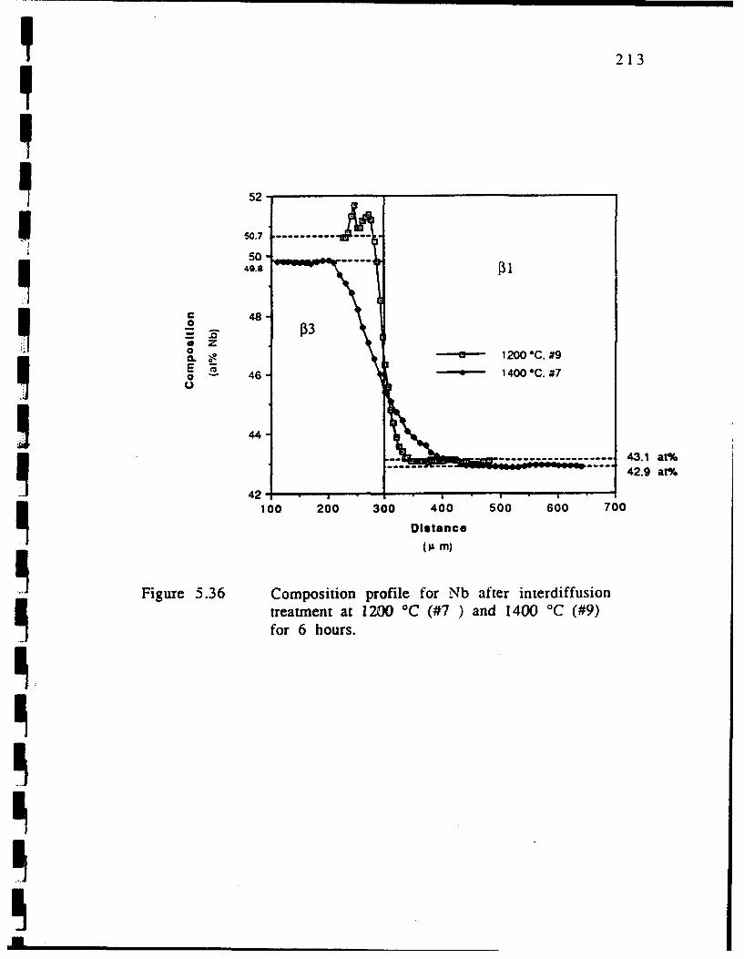
213
52
I 50.7
50-49.8 1
0 48 3
0 ,, ' --- 1200 "C. #9E Z 46- 1400 *C. #70
44- ---- --------- 4 43.1 at%
P 42 .Io
100 200 300 400 500 600 700
Distance
Figure 5.36 Composition profile for Nb after interdiffusiontreatment at 1200 *C (#7 ) and 1400 0C (#9)for 6 hours.
.1
Ii

p 214
15250.2 .. . .. .
49.3------ ---- -----------• ~48-•t
c
0 46- a. • ' - 1"-00 *C. #7
0 1 290 °C #9
9 42-Markers ----- ---------------------- 41.1 at%Plane
40 Pa ----------- - --------------- 40.1 at%
100 200 300 400 500 600
Distance
Figure 5.37 Composition profile for Ti after interdiffusiontreatment at 1200 'C (#7) and 1400 'C (#9) for 6"hours.
p.III
.I
I

215
2
M -0
M -t 00
C)) -ýC 0 a
-n CK-e
0
(U -n 0 C1 I"-T4)e4
o F-
4C)
fn0-o orC-,c
4)4CN4m) -=C

216
b) •._I•_ (1200 °C):In this case the solidus temperatures of the two
sides are not expected to be very different, and therefore the
concentration gradients of the components play an important role in
the final shape of the penetration curve. Aluminum is the element
with the largest composition gradient and penetrates from the j01 to
the 133 side producing an approximately similar penetration depth on
both sides of the couple. The flux opposite to the Al motion is mainly
due to Ti, as indicated by the small penetration of Nb in the 131 side.
It is interesting that Al penetration depth in the 133 side is much
smaller than the draw depth of Nb and Ti. A comparison of the
diffusion zone size with that at 1400 'C for the same couple reveals
that the apparent draw depth of Nb on the 533 side decreases with
increasing temperature. This observation suggests that indeed the
U. apparent draw depth of Nb at 1200 *C does not represent the actual
physical motion of Nb. However, since Al does not penetrate to the
same depth, unless the crystal can tolerate very large fractions of
vacancies there should be an actual uphill diffusion of Nb. Another
possibility that can contribute to this observation is a large
composition dependency of the molar value in this system.
Unfortunately no precise lattice paramenter data for these
compositions are known. Here, the Ti comes from a large distance
within the 033 side. The apparent large penetration depth of Nb on the
133 side is due to the readjustment of the atomic fraction due to the
lost of Ti. It should be noted that the penetration depths evaluated
by microprobe analysis may not represent the physical distance that
atoms have moved, since a variation in their atomic fraction may beUI

F 217
a result of the diffusivity of any of the other species in that part of
tl:e couple [69].
c) D.l.Ti (1200'C): The relative penetrations of Al and Ti are equal on
each side of this couple and larger than that of Nb. It is observed
again that the side with the lower solidus temperature (Ti-side)
exhibits the larger penetration depths. The depths of penetration in
this case are in general much larger as compared to those in the
P131/Nb couple. In the latter the kinetics are limited by the motion of
atoms and vacancies in the Nb side, however, in the former couple it
is the motion in the 131 side that controls the penetration.
d) . (1200 QC): In this case the penetration depth of Al is smaller
that the P1/133 couple due to a smaller Al concentration gradient. It is
interesting to note that in this couple, contrary to the 131/133 couple
the Nb and Ti draw depths are much smaller and equal to the
penetration depth of the Al on the 133 side. This behavior may be
related to the lower concentration gradient of Ti in the 132/133 coupleI• than in the P1/133 couple.
e) 1j_!_.- (1200 'C): This couple exhibits similar behavior to the 131/Nb
couple analyzed previously. Here, basically the penetration depth of
the elements is controlled by the motion of Nb in the Nb-rich side,
which has the higher solidus temperature.
f) A.j/Nb (1400 °C): The behavior of this couple is similar to that
observed in the same system at 1200 °C, except that, as expected,
larger penetration depths for each component are obtained.
e) A.0_4- (1400 °C): At 1400 *C the mobility of Al is higher, and
consequently the penetration depth of it is larger. At this
temperature Ti penetrates deeper into 13i side, however, its draw
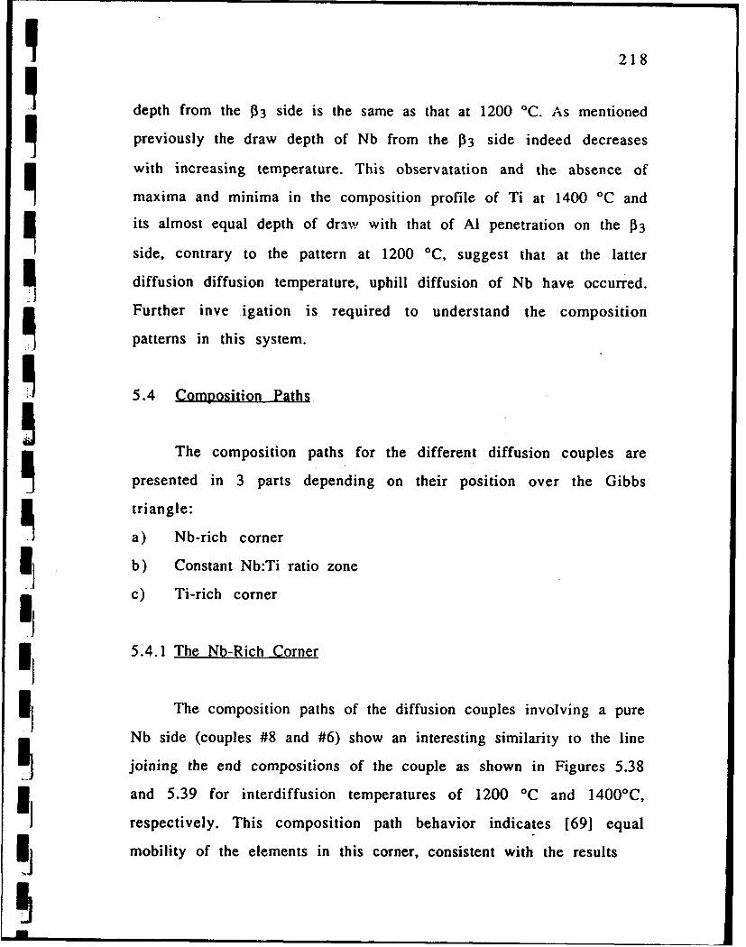
218
depth from the 03 side is the same as that at 1200 'C. As mentioned
previously the draw depth of Nb from the 033 side indeed decreases
with increasing temperature. This observatation and the absence of
maxima and minima in the composition profile of Ti at 1400 'C and
its almost equal depth of draw with that of Al penetration on the P3
side, contrary to the pattern at 1200 0C, suggest that at the latter
diffusion diffusion temperature, uphill diffusion of Nb have occurred.
Further inve igation is required to understand the composition
patterns in this system.
P 5.4 Composition Paths
I The composition paths for the different diffusion couples are
presented in 3 parts depending on their position over the Gibbs
triangle:
a) Nb-rich cornerp b) Constant Nb:Ti ratio zone
* c) Ti-rich corner
* 5.4.1 The Nb-Rich Corner
The composition paths of the diffusion couples involving a pure
Nb side (couples #8 and #6) show an interesting similarity to the line
joining the end compositions of the couple as shown in Figures 5.38
and 5.39 for interdiffusion temperatures of 1200 °C and 1400'C,
respectively. This composition path behavior indicates [69] equal
3] mobility of the elements in this corner, consistent with the results

1 219
I60
p /V
Nb 060
pFigure 5.38 Composition path for diffusion couple #8 (131/Nb),S~and schematic representation of the crossover
displacement. £ Middle point composition.
0 Matano plane composition.
p |
pApV Vp//// V //////P1\ //A/I/V \///-
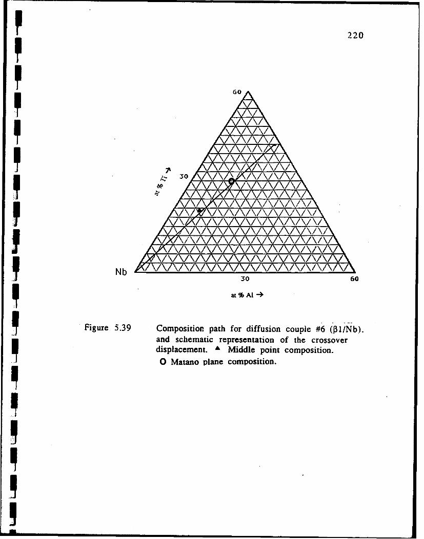
P 220
6A
• 30
,~\V X/\,v /VV /\l/Z\
30 60
aIAI4
Figure 5.39 Composition path for diffusion couple #6 ('O1/Nb).S~and schematic representation of the crossover
displacement. A Middle point composition.1 O0 Mano plane composition.
IFiue53.opstonpt o ifso cul 6(31N)
an ceai ersnaino h rsoedipaeet £Mdl ontcmoiin

I 221
I shown in Table 5.1. The composition path for the other couple in this
corner, #11 (Figure 5.40), shows a visible bending of the path with a
crossover point close to the A52 composition. In this couple the Al
concentration gradient is almost zero, however,, as shown in Figure
5.29 there is an apparent redistribution of Al possibly due to
unequal mobility of Ti and Nb in this couple.
5.4.2 The Constant Nb:Ti Ratio Zone
For this section the composition paths for diffusion couples #10,
#9 and #7, which are given in Figures 5.41, 5.42 and 5.43
respectively, are considered. The similarity of the composition paths
for these 3 couples is evident. Both ends of the composition paths are
directed toward the Ti corner and the midsection at the crossoverseems to follow a path parallel to a constant Ti composition.
5.4.3 The Ti-Rich Corner
There is only one composition path for the discussion of the
diffusivity behavior in this corner (couple #12). The pattern followed
by this path is somehow similar to that obtained for couple # 11, but
with a more pronounced tendency to deviate from the line
connecting the composition ends and it bends toward the Nb-Ti side
of the couple as shown in Figure 5.44. A high magnification of the
path near the Ti corner is shown in Figure 5.45. It is observed from
these Figures that the end of the paths at both ends point toward the
Al corner of the Gibbs triangle, which implies that Al moves faster
Ii

I 222
I 60
,•30I
dX) /V 7,///\/\ /V
4ý ~ ~ a AIA( "•\-\~
II
Nb30 60
at %Al4
Figure 5.40 Composition path for diffusion couple #11(J30/f32).and schematic representation of the
crossover displacement. A Middle point
composition. 0 Matano plane composition.

P 223
PAX X
ir %f%1"' \ / \f f \/I \ 1%
V V
550
I % AI -10
Figure 5.41 Composition path for diffusion couple #10
(133/012), and schematic representation of the
crossover displacement. & Middle point
composition. 0 Matano plane composition.
pII

224
1 60
7 V! -. 50-VAV
I-
40 20
at % Al -
Figure 5.42 Composition path for diffusion couple #9(0•3113/1), and schematic representation of thecrossover displacement. A Middle pointcomposition. 0 Matano plane composition.p
III
I MI

p 225
71 V650
V P\ /
S~40
to 20
a/\ /l
Figure 5.43 Composition path for diffusion couple #7 i n o
I the crossover displacement.
A Middle point
composition. 0 Mat~ao plane compo~sition.
,I
IIII III I 1 I I
III III I
a z %i -l i l i i i i i l H

I 226
I Ti
p AA/
/-N7-\//\/\/\/ VI
30 60
at% Al --
Figure 5.44 Composition path for diffusion couple #12(Pl/Ti, 1400 °C), and schematic representation ofthe crossover displacement. & Middle pointcomposition. 0 Matano plane composition.iI
iI
I!

P 227
P1-il-l
I I
3.0 /\ ./ / ! /\/\ / \ /•, \/\/\/\/ /
1.5 3.0
.I IJ couple #12 (131/Ti).
Iii
IVIVIA
IVIN
I 228
than Nb. The relative mobility of Ti and Al may be deduced by the
displacement of the crossover point toward the Ti cornei suggesting
a relative higher mobility of Ti. This matter will be discussed later in
detail (section 5.6).
5.5 Kirkendall Shifts
Two different methods were employed to measure the
Kirkendall shift in the systems under study. The first of them was
done experimentally by measuring the distance between the two
interfaces present in the sandwich-like couples before and after the
diffusion treatment. The resultant difference was then divided by 2
to get the net displacement of the markers. The second methodI employed the same computer program used for the evaluation of the
Matano Interface in the bin,-ry system. In this case, the Matano
plane determination was conducted over the profiles of the 3
components for each diffusion couple. In general, the calculated
Matano interface position was approximately the same for the three
elements. Table 5.2 shows the Kirkendall shift as calculated by the
above mentioned methods. There is an excellent agreement between
the two methods, except for the couple #11 (032/h0), for which both
methods show similar displacements but in opposite directions. It
was observed that the agreement between results of both methods is
better when the computer program was applied to the experimental
Al composition profiles. The reason for this could be the absence of
critical points in the Al profiles in most cases. One problem associated
I with the experimental method was the lack of statistical
IJ

229
p* 44 -P+ -§. (t-- 0
c~cn
U -^-
uA 00 __O)
- U - Co+. cH el-E -H H H 0-- - 40 44 H H
cm Z- C-4 C= ~ 0l mp .~~~ z ~ -

P 230
measurements as only a few number of yttria markers were
available. For the case of couple #12, they were not even found as
they were probably dissolved in the Ti matrix. Instead, in this case
I the measurements were made using oxide markers developed in the
bonded interface during the hot-pressing operation.
At 1200 °C, the diffusion couple with pure Ti (#12) shows the
I largest displacement observed with a Kirkendall shift toward the Ti
side of the couple. Regarding the two 1400 *C treated couples, a
significant marker displacement (Kirkendall shift) was observed for
couple #6 pointing toward the ternary side of the couple (rich Ti,
poor Nb). As to the other couple treated at 1400 *C (#7) and those
interdiffused at 1200 'C, the Kirkendall shift is small and in some
cases negligible. For example, the 131/033 couples with constant Nb:Ti
I• ratio and 15 at% Al (couples #7 and #9) exhibited a negligible
displacement of the markers at either temperature, 1400 'C or 1200
*C. Assuming only the Al composition gradient, then one would
expect a larger shift in the 0b/133. couple than in the P3/P2 couple
(5at% Al). However, the consideration of the increase in Nb and Ti
gradients suggests that more Nb and Ti flow into the ternary side in
the 03/031 couple than they do in the 33/I2 couple.
* 5.6 Crossover Displacements
As mentioned in Chapter 2, the crossover point of a
composition path in the Gibbs triangle is displaced from the mid
point of the line connecting the end compositions when the5 penetration tendencies of the components are concentration-

P.. "1 231
dependent. The composition of the crossover point should correspond
to the composition of the original weld interface, which is given by
the composition of the Matano interface. In Figures 5.38 to 5.44 the
Matano interface compositions are marked on the composition paths.
There is a good correlation between the calculated and crossover
compositions, mainly in the couples involving 13 , P2, and J03 alloys.
S5.6 Discussion
The discussion of the diffusivity in the ternary Nb-Ti-AI 13-solid
solution is based on the results obtained for penetration tendencies
(see Table 5.1), composition paths (see Figures 5.38-5.45), and
Kirkendall shifts (see Table 5.2). An analysis of the composition
Sprofiles permitted to evaluate the approximate penetration ratios of
the components in the different couples. These ratios are given in
Table 5.3, and it can be observed that they depend strongly on the
composition of the alloys. The discussion of these results will be
focused on three different regions and emphasis will be placed on
the diffusion composition patterns following DeHoff et. al. [69].
a) Nb/Ti Constant Ratio
The composition paths of the 3 couples in this region (#10, #9,
#7) as shown in Figures 5.41 to 5.43 are similar in behavior. It is
observed that the end segments are directed toward the Ti corner,
therefore, indicating that Ti is the fast diffuser. The midsection of
these paths are parallel to the Nb-Al side suggesting that Al and Nb
have similar penetration tendencies. When the midsections of the
133/131 couples annealed at two temperatures are compared in more

p 232
p0
p>0
.0 co - 1 - 4
02..1Z 00I-1m cm-4 en cm CR

I 233
detail (#7 and #9), it is observed that the midsection of couple #7
(1400 'C) presents a slight rotation toward the Al corner, suggesting
that the mobility of Nb increases as the temperature increases. It is
also observed that deviation of the composition path from the
straight line behavior in couples #7 and #9 decreases with increasing
the annealing temperature, which suggests that the mobility of Al
and Nb is closer to that of Ti at higher temperatures.
As far as the penetration tendency ratios are concerned (Table
5.3), the three couples show the highest penetration ratio for the
element Ti, consistent with the observations regarding the
composition paths. However, when the ratios for Nb and Al are
compared, an artificially large penetration of Nb is found for the
031/133 couple (#9) annealed at 1200 *C. As demonstrated by DeHoff et.
al. 169), the penetration depths calculated from the microprobe
analysis, particularly for elements that are not indeed mobile, do not
represent the physical distance over which the elements have
I moved. In this case the imbalance in distribution of Al and Ti alters
the percentage of Nb. This ;s supported by the facts that Nb shows a
larger depth at 1200 0C than it does at 1400 'C in the 03 side, and
that the reaction depth of Ti at 1200 'C is much larger than that of
Al.
A comparison of the penetration depths for I31/03 and 032/03
couples (Table 5.1) reveals that in general the depths are much
larger for the 131/133 couple, which had a larger concentration gradient
of the elements. The penetration depth of Al on the P33 side (Nb-50Ti)
decreases from 72 gtm to 31 gtm with a decrease in concentration
gradi-nt. It is interesting to note that the Nb and Ti are apparently
p. 234
drawn from much deeper in the 031/133 couple, however, in the 02/53
couple their depth or Iraw is similar to the penetration depth of Al.The larger depth of draw of Ti in the P 1/53 couple can be attributed
to the larger concentration gradient of this element in comparison tothe 132/133 couple. Consistently, in both couples Nb penetrates to ashorter depth into the counterpart side of the P3 than does Ti.
As far as Kirkendall shift for these couples are concerned, thedisplacements were measured to be very small but always toward
the ternary side, indicating that physically more Al atoms weretransferred to the 03 side. This observation is consistent with the
larger concentration gradient of Al than those of Ti and Nb for these
couples.
b) Ti Corner
In consistency with the assumption that Ti moves much fasterthan Al and Nb the composition path of P3/Ti couple (couple #12)
showed the tendency toward a straight line behavior (see Figure
5.44). The end segment at the P33 composition is directed toward theAl corner indicating that in this corner Al moves faster than Nb.
Consequently the composition path deviates slightly from thestraight line behavior, but due to a much faster diffusivity of Ti it
crosses over very close to the Ti corner.
t The system, in general, shows the highest penetration depths in
this corner consistent with the fact that Ti has the lowest meltingpoint among all constituent alloys used in this study. As shown infable 5.1 all elements show a larger depth of diffusivity in the Ti
side than in the 031 side consistent with the high solidus temperatureI

P 235
of the latter alloy. Nb tends to show shorter draw and penetration
depths than Ti and Al do.
The Kirkendall Shift measured in this couple is also one of the
largest observed in all couples, and accordingly, it predicts a larger
I flux of Ti into the 01 side of the couple.
c) Nb CornerI The penetration ratio values (1:1:1) given in Table 5.3 for
couples #6 and #8 are in complete agreement with the matching of
composition paths to the straight line connecting the end
compositions observed for these couples. This behavior can be
interpreted as a result of the low jump frequencies of all three
components in this region of the diagram, which again can be
correlated to the solidus temperature of the alloys involved and is
supported by the depth of penetration measured on the two sides of
the couples. These penetrations consistently show a very small
penetration into the Nb side and it is the same for the three
elements. The penetration depth in the P1I side, on the other hand
shows a deeper diffusion region due to the lower solidus
temperature of this alloy. The low value of the Kirkendall shift
observed at 1200 'C also shows that the mobility of the three
elements is similar. However, when the temperature is increased to
1400 °C, the Kirkendall shift measured is very large (see Table 5.2),
which is difficult to interpret since it indicates that a large
N displacement of Ti and Al atoms toward the Nb had occurred. Such
observations do not agree with the composition path and the
penetration depth results. Further investigation is required to
N resolve these inconsistencies.

P 236
The results of this study suggest that the diffusivity of the
components in general is larger when the amount of titanium present
in a couple increases. The Kirkendall shift and crossover point
displacement results also indicate that the mobility of the system
increases as the titanium content increases, but they also suggest
that the aluminum owns a larger mobility than niobium as both the
II Kirkendall shift and crossover displacement point opposite to the
niobium corner. In accordance with these results, titanium owns the
largest jump frequency followed by aluminum and the niobium.
Another observation of this study is that the Kirkendall and
crossover shifts are in agreement as to the direction of the
displacement, and the composition at the Matano interface correlates
well with the crossover composition. The mobility of all components
is larger close to the Ti corner of the diagram. The jump frequency of
the system changes more drastically as going from the Nb corner side
of the system toward the Ti corner. This behavior causes, therefore, a
similar crossover shift in the couples involving end compositions in
the Ti-rich section of the ternary system, and a larger crossover shift
in the couples involving Nb-rich end compositions.
5.7 SummaryIContrary to the behavior of Nb-4.5 at% Al solid solution, no
propensity to internal oxidation was detected in the ternary alloy.
This observation suggests that the addition of Ti reduces the
susceptibility of the alloys to internal formation of A1203. Despite the
Sobservation of two-phase microstructures at room temperature, it

238
CHAPTER 6
CONCLUSIONS
The diffusion behavior in the binary Nb-Al and the ternary Nb-
Ti-Al systems were studied employing Matano-Boltzmann diffusion
couple method. The results obtained have led to the following
conclusions:
1- The binary Nb-4.5at% Al alloy was very susceptible to internal
oxidation. However, the addition of Ti to the b.c.c. solid solution
.I completely retarded the internal oxidation.
2- The zirconia particles used as markers, were unstable in the Nb-Al
P3 solid solution and lecomposed at high temperatures. The
substitution of the markers with yttria proved that this oxide is
completely inert in the binary Nb-Al P3-solid solution, however, in the
presence of Ti some reactivity was observed.
3- The interdiffusion coefficient of the binary Nb-Al system varied
linearly with composition in the range of 1-3 at% Al and it showed a
linear Arrhenius behavior as a function of temperature. The average
interdiffusion coefficient in the temperature range of 1350 'C to
1550 *C can be expressed through the following equation:
D = 0.1136 exp (-80,105 (cal/mole)/RT) cm2 /sec
The activation energy was independent of the composition in the 1-3
at% range. The average intrinsic diffusivity of Al in the same

239
temperature range, calculated based on a dilute solution assumption
I is given by:
DAI = 0.1161. exp (-80,165 (cal/mole)/RT) cm 2 /sec
4- Kirkendall shift measurements correlate well with the calculated
I crossover displacements in the ternary Nb-Ti-AI system. The
direction and magnitude of displacements in conjunction with an
analysis of the composition paths suggest that Ti is the fastest
component of the system at all compositions, with a very small
difference in the relative mobilities of Al and Nb. The addition of Ti
increases the general diffusivity of the system partially due to a
reduction in the solidus temperature of alloys.
5- The occurrence of maxima and minima in the composition profiles
obtained by microprobe analysis correlates with the existence of
small composition gradients or very low relative mobilities.
6- Results of this study show that the 3 elements Nb, Ti and Al, have
similar but very low jump frequencies in the Nb -rich corner of the
Gibbs triangle. In the Ti-rich corner the jump frequencies of these
elements are unequal but much higher than the Nb jump corner. Ti
I has the highest jump frequency in this corner.
MIIIU
I
II
APENI
PRBESASCAEIIHTEMAUEETO OPSTO
IRFLSB IRPOEAAYI
I--24

p 241
APPENDIX A
PROBLEMS ASSOCIATED WITH THE MEASUREMENT OF COMPOSITION
I PROFILES BY MICROPROBE ANALYSIS
The evolvement of electronic analysis techniques such as the
Electron Microprobe for the study of diffusivity process have
provided the capability to measure gradient concentrations at very
low spatial resolutions (Ilim) that traditional techniques would have
never been able to reach. This has permitted to study diffusion at
very short scales, such as low temperature and/or short time
treatments. However, the success of the application of this technique
relies on the accuracy of the data obtained. In order to report
I reliable results, several composition profiles were measured in each
of the diffusion couples studied in this research. At least twop matching profiles were obtained for each couple (Figures A.1), and
-- the one with the smoother curve was chosen for calculating of the
Matano plane position.
The inconsistency in composition profiles obtained for an
element in the same couple was found to occur in two ways.
Sometimes a constant shift in the composition profile was detected.
Due to a change in parameters associated with the calibration of the
instrument, the entire profile was shifted with respect to the initial
profile. Since this displacement was equal for all compositions, no
effect on the calculated depth of penetration was -detected. The

242
20O
... 16.8 at%
Markers Plane
ICCL
0a * 10
-U--Profile 112 30 Profile 2
40
I C." I100 200 3;0 400 500
l Distance
Figure A4 Composition profiles of Al after interdiffusioni treatment of couple #9 at 1200 0C for 6 hours.
II
I=

243
computation of the Matano interface was not affected either, since
the end compositions employed in such calculations were those
obtained while measuring the resulting composition profiles. Figure
A2 shows this behavior for the Nb composition profiles in couple #9.
The other effect on the measurement of the composition profiles was
that due to the existence of markers close to the point from which
I the profile was obtained. Figure A3 shows the BSE micrograph of a
diffusion profile measured in diffusion couple #10 and the presence
of yttria markers. When the microprobe analysis of the couple was
performed, the closeness of the markers produced compositions
profiles as that shown in Figure A4.a. When the analysis was
performed in zones far enough from the markers, normal profiles as
i that shown for the same couple in Figure A4.b was obtained.
IJ
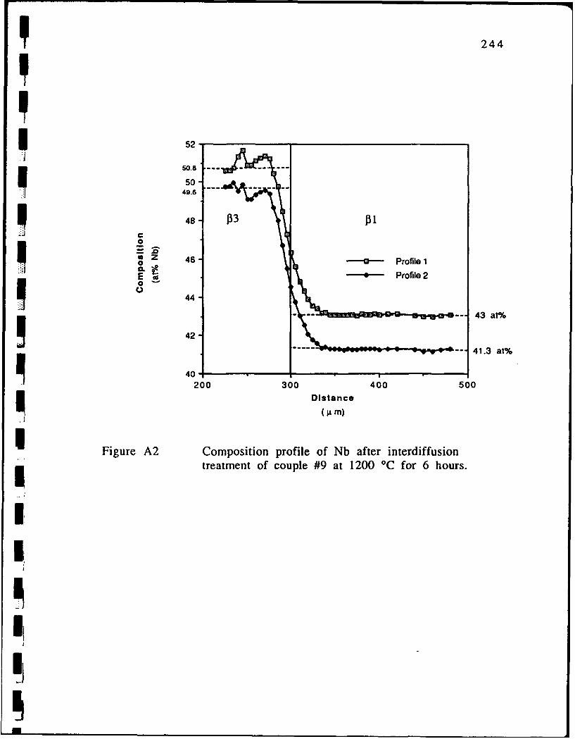
SI 244
* 52'
50.8
5049.6
48 033 031C
46 ----- Profile 1-c-- Profile2
44
-- 43 at°/9
42 41.3 at%
40'200 300 400 500
Distance
(A m)
1 Figure A2 Composition profile of Nb after interdiffusionp treatment of couple #9 at 1200 *C for 6 hours.
I.I

P •245
P10 PM
SFigure A3 BSE micrograph showing microprobe analysis
i .... contamination close to yttria markers in couple
#I

I 246
,5 o5
50
-- ------ ----49 -- a)
E b)0
48-
4 47.2 at%
100 200 300 400 500
Distance
, (j m)
I Figure A4 Composition profiles of Nb after interdiffusiontreatment of couple #10 at 1200 'C for 6 hours.a) Measured close to yttria markersb) Measured away from markers.
IIIIIU

I
REFERENCES
[1] P. Kofstad, and S. Espevik, J. Electrochem. Soc., 112 (2) (1965),pp.153-160.
[2] J. F. Brady, J. N. Ong, Jr. "Oxidation Rate of Nb as a Function ofTemperature and Pressure", Columbium Metallurgy, 10, Ed.Interscience, NY, (19ý0), p. 719.
[3] H. Inouye, "Nb in High Temperature Applications", Proceeedingsof the International Symposium Niobium '81, Ed. H. Stuart, AIME,Warrendale, Pa.
[4] R. A. Perkins, G. H. Meier, K. T. Chiang, "Effect of Alloying. RapidSolidification. and Surface Kinetics on High TemperatureEnvironmental Resistance of Nb" , LMSC-F195926 Report forAir Force Office of Scientific Research under contract F49620-86-C-0018, (June 15, 1987).
[51 R. C. Svedberg, "Oxides Associated with the Improved AirOxidation Performace of some Nb and Intermetallics and Alloys".Properties of High Temperature Alloys, Z. A. Foroulis and F. S.Pettit eds., Electrochemistry Society 1976, p. 331.
[6] G. I. Nikolaev, N. V. Bodrov, Zh. Fiz. Khim., 52 (1978), p. 1430.
[7] E. 0. Kirkendall, and, A. D. Smigelskas, Trans. AIME, 171 (1947),p. 130.
5 [8] P. G. Happoldt, Master of Sc. Thesis, University of Purdue, 1988.
[9] J. L. Murray, "Phase Diagrams of Binary Ti Alloys", Ed. J. L.Murray, ASM Intern., Metals Park, OH, (1987), p. 188.
[10] C. E. Lundin, A. S. Yamamoto, Trans. AIME, 236, (1966), p. 863.
[11] J. L. Murray, "Phase Diagrams of Binary Ti Alloys", ed. J. L.Murray, ASM Intern., Metals Park, OH, (1987), p. 173.
247

248U[121 J. H. Perepezko, Y. A. Chang, L. E. Seitzman, J. C. Lin, N. R. Bonda,
T. J. Jewet, J. C. Mishurda, "High Temperature Phase Stability inthe Ti-Al-Nb System". High Temperature Aluminides andIntermetallics Proc. Symp. Indianapolis, Ind., Oct. 1989ASM/TMS-AIME.
[13) K. Kaltenbach, S. Gama, D.Pinatti, K. Schulze, E. Henig, Z.Metallkde., 80, (1989), p. 535.
[14] L. Bendersky, W. Boettinger, "Investigation of B2 and RelatedPhases in the Ti-Al-Nb Ternary System", Mat. Res. Soc. Symp.Proc., 133, (1989), p. 45.
[15] T. J. Jewett, J. C. Lin, N. R. Bonda, L. E. Seitzman, K. C. Hsieh, Y. A.Chan, "Experimental Determination of the Ti-Al-Nb PhaseDiagram at 1200 *C", Mat. Res. Soc. Symp. Proc. 133, (1989), p.69.
[16] A. D. LeClaire, "Diffusion in B.C.C. Metals", A.S.M., Cleveland Ohio,(1965).
[17] G. Newmann, V. Tolle, Phil. Mag. A, 54, (1986), p. 619.
[18] J. F. Murdock, T. S. Lundy, E. E. Stanbury, Acta Metall., 12,(1964), p. 1033.
[19] G. Kidson, Canad. J. Phys., 41, (1963), p. 1563.
[20] W. Petry, T. Flottmann, A. Heiming, J. Trampenau, M. Alba, G.Vogl, Phys. Rev. Lett, 61, (6), (1988), p. 722.
[211 C. Herzig, U. Kohler, Mater. Sci. Forum, 15/18, (1987), p. 301.
[22] W. Bussmann, C. Herzig, H. A. Hoff, J. N. Mundy, Phys, Rev. B, 23(12) (1981), p. 6216.
[231 R. E. Eizinger, J. N. Mundy, H. A. Hoff, J. Nucl. Matl., 69/70,P (1978), p. 523.
I [24] A. E. Pontau, D. Lazarus, Phys. Rev B, 19, (8), (1979), p. 4027.
[25] S. L. Sass, J. Less-Common Met., 28, (1972), p.157.
I)

I 250
[42] R. J. Lauf, Report 1978, COO-1198-1216,104pp. Avail. NTIS.From Energy Res. Abstr., 4, (6), (1979), Abstr. # 14004.
[43] G. Canelli, R. Cantelli, Hydrogen Met., Proc. Int. Congr., 2nd,1977, 1, Paper 1B2, 5 pp., Pergamon Press: Oxford, England.
[44] W. S. Gorsky, Phys. Z. Sowjetunion, 8, (1935), p. 457.
U [45] J. F. Stringer, "High Temperature Corrosion of AerospaceAlloys". AGARD-AG 200, Advisory Group for AerospaceResearch and Development, NATO, Augost 1975.
[46] N. Birks, G .H. Meier, "Introduction to the High TemperatureOxidation of Metals", Edward Arnold, Ltd; London, 1958.
[47] F. Gesmundo, F. Viani, Oxid. Metalls. 25, (1986), p. 269.
[48] C. Wagner, Z. Elektrochem., 63 (1959) p. 772.
[49] K. Kirano, Y. Ijima, "Inter- and Reaction Diffusion betweenAlloys of very Different Diffusional Properties". Diffusion inSolids: Recent Developments, M. A. Dayananda & G. E. Murcheds., AIME, 1985, p. 14 1.
[50] J. E. Morral, M. S. Thompson, 0. J. Devereux, Scripta Met., 32(1986), p. 1562.
[51] R. C. Frank, R. J. Lauf, C. J. Alstetter, Met. Trans. A, 13A, (4),(1982), p. 539.
[52] B. D. Bastow, G. C. Wood, D. P. Whittle, Corros. Sci., 25, (1985), p.253.
[53] J. A. Nesbit, R. W. H-,ckel, "High Temperature Protective3 !Coatings", ed. S. C. Singhal, AIME, (1984), p. 75.
[54] A. Fick, "Uber Diffusion", Poggendorffs Annalen, 94 (1855),p. 59.
[55] L. Boltzmann, Ann. Phys., Leipzig, 53 (1894), p. 959.
[56] C. Matano, Japan Journal Phys., 8 (1933), p. 109
BIOGRAPHICAL SKETCH
Jose Guadalupe Luis Ruiz Aparicio was born on February 28,
1960, in Mexico City, D.F., Mexico. He received his elementary and
S~secondary school there, graduating from C.C.H. High School in 1977.
In 1985 Mr. Ruiz graduated ,with honors from Universidad Nacional
Autonoma de Mexico (National University of Mexico), Mexico City,
Mexico, with a degree in Chemical Metallurgical Engineer.
In 1982 he joined the faculty of the Universidad National
Autonoma de Mexico as Assistant Professor in the Department ofChemical Metallurgical Engineering. From 1982 to 1987 he worked
S~there in the area of Physical Metallurgy.
He joined the mechanical metallurgy group in the DepartmentS~of Material Science and Engineering, University of Florida in 1988.
I Since then he has pursued work toward the degree of Master of
Science and Engineering. After graduation, he will pursue work
toward the degree of Doctor of Philosophy in Materials Science and
Engineering at the University of Pittsburgh, He plans to•, reincorporporate to the National University of Mexico afterwards.
S~The author is married to former Laura G. Barquera Lopez from
Mexico city, Mexico. He is member of the TMS and ASM.
S~253