Embed Size (px)
Citation preview

Mirror-Stratifiable Regularizers
Jerome MALICK
CNRS, Laboratoire Jean Kuntzmann, Grenoble
Based on joint work with
Guillaume Garrigos Jalal Fadili Gabriel Peyre
Outline
1 Example in inverse problems (context and existing results)
2 Mirror-stratifiable functions
3 Optimization with mirror-stratifiable regularizersSensitivity under small variationsActivity identification of proximal algorithmsModel recovery in inverse problemsModel consistency in learning
4 Numerical illustrations
Example in inverse problems (context and existing results)
Inverse problems
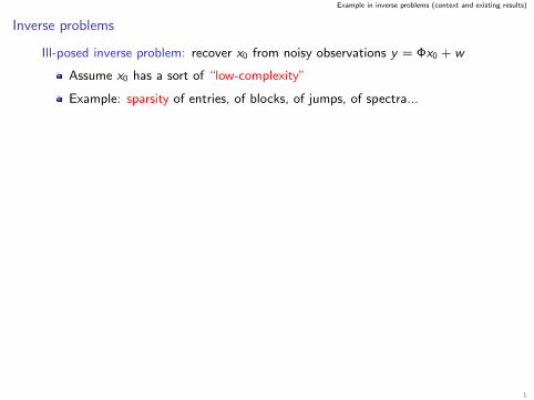
Ill-posed inverse problem: recover x0 from noisy observations y = Φx0 + w
Assume x0 has a sort of “low-complexity”
Example: sparsity of entries, of blocks, of jumps, of spectra...
Regularized inverse problems
minx∈RN
1
2‖y − Φx‖2 + λR(x)
data-fidelity regularization
R promotes low-complexity to solutions (similar to the one of x0)
λ > 0 controls trade-off (depends on noise level ‖w‖ and R(x0))
Questions: for a solution x(y , λ)
Under which conditions, can we guarantee
1 `2-recovery ‖x(λ, y)− x0‖ = O(‖w‖α) ?
2 model recovery the low-complexity of x(y , λ)coincides with the one of x0 ? (when w small)
1

Example in inverse problems (context and existing results)
Inverse problems
Ill-posed inverse problem: recover x0 from noisy observations y = Φx0 + w
Assume x0 has a sort of “low-complexity”
Example: sparsity of entries, of blocks, of jumps, of spectra...
Regularized inverse problems
minx∈RN
1
2‖y − Φx‖2 + λR(x)
data-fidelity regularization
R promotes low-complexity to solutions (similar to the one of x0)
λ > 0 controls trade-off (depends on noise level ‖w‖ and R(x0))
Questions: for a solution x(y , λ)
Under which conditions, can we guarantee
1 `2-recovery ‖x(λ, y)− x0‖ = O(‖w‖α) ?
2 model recovery the low-complexity of x(y , λ)coincides with the one of x0 ? (when w small)
1
Example in inverse problems (context and existing results)
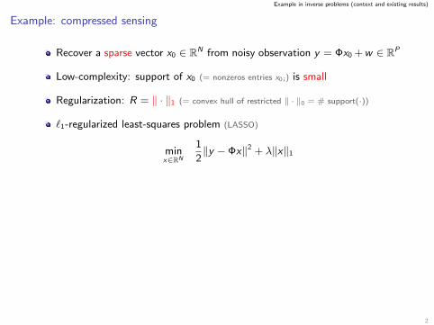
Example: compressed sensing
Recover a sparse vector x0 ∈ RN from noisy observation y = Φx0 +w ∈ RP
Low-complexity: support of x0 (= nonzeros entries x0 i ) is small
Regularization: R = ‖ · ‖1 (= convex hull of restricted ‖ · ‖0 = # support(·))
`1-regularized least-squares problem (LASSO)
minx∈RN
1
2‖y − Φx‖2 + λ‖x‖1
A lot of research on recovery e.g. [Fuchs ’04] [Grasmair ’10] [Vaiter ’14]...
For Φ gaussian [Candes et al ’05] [Dossal et al ’11]
“we have recovery when P is large enough”
`2-recovery when P = Ω(‖x0‖0 log(N/‖x0‖0))
model recovery when P = Ω(‖x0‖0 log N)
What happens if P is not large enough ?
2

Example in inverse problems (context and existing results)
What happens in degenerate cases ?
real-life problems are often degenerate (e.g. medical imaging)...
...but all existing results assume some kind of non-degeneracy
In particular: the previous ones + [Lewis ’06] (general sensitivity) + [Bach ’08]
(trace-norm recovery) + [Hare-Lewis ’10] (identification) + [Candes-Recht ’11]
(recovery) + [Vaiter et al ’15] (partly-smooth recovery) + [Liang et al ’16]
(identification of proximal spitting), and many others...
Position of our work on this topic
– known results
non-degenerate problem =⇒ (exact) recovery
– in this talk
general problem =⇒ some recovery ?
Yes ! for some structured regularizations
(that we called mirror-stratifiable)
J. Fadili, J. Malick, and G. Peyre
Sensitivity Analysis for Mirror-Stratifiable Convex Functions
Accepted in SIAM Journal on Optimization, 2018
3

Outline
1 Example in inverse problems (context and existing results)
2 Mirror-stratifiable functions
3 Optimization with mirror-stratifiable regularizersSensitivity under small variationsActivity identification of proximal algorithmsModel recovery in inverse problemsModel consistency in learning
4 Numerical illustrations
Mirror-stratifiable functions
Recall on stratifications
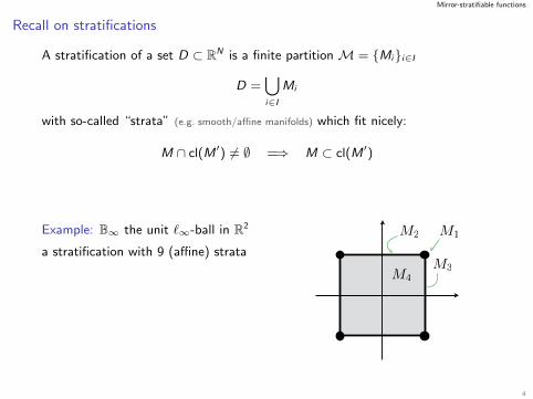
A stratification of a set D ⊂ RN is a finite partition M = Mii∈I
D =⋃i∈I
Mi
with so-called “strata” (e.g. smooth/affine manifolds) which fit nicely:
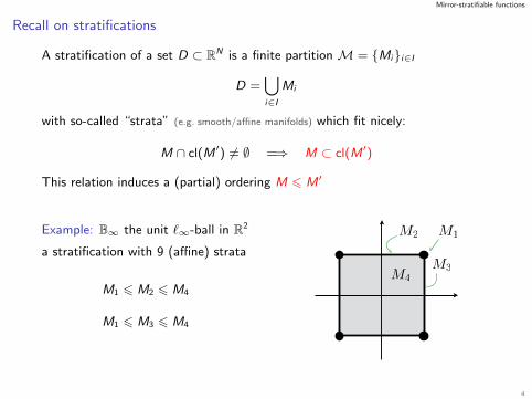
M ∩ cl(M ′) 6= ∅ =⇒ M ⊂ cl(M ′)
This relation induces a (partial) ordering M 6 M ′
Example: B∞ the unit `∞-ball in R2
a stratification with 9 (affine) strata
M1 6 M2 6 M4
M1 6 M3 6 M4
M1M2
M3M4
4
Mirror-stratifiable functions
Recall on stratifications
A stratification of a set D ⊂ RN is a finite partition M = Mii∈I
D =⋃i∈I
Mi
with so-called “strata” (e.g. smooth/affine manifolds) which fit nicely:
M ∩ cl(M ′) 6= ∅ =⇒ M ⊂ cl(M ′)
This relation induces a (partial) ordering M 6 M ′
Example: B∞ the unit `∞-ball in R2
a stratification with 9 (affine) strata
M1 6 M2 6 M4
M1 6 M3 6 M4
M1M2
M3M4
4

Mirror-stratifiable functions
Mirror-stratifiable function: formal definition
A convex function R : RN→R ∪ +∞ is mirror-stratifiable with respect to
– a (primal) stratification M = Mii∈I of dom(∂R)
– a (dual) stratification M∗ = M∗i i∈I of dom(∂R∗)
if JR has 2 properties
JR :M→M∗ is invertible with inverse JR∗
M∗ 3 M∗ = JR(M) ⇐⇒ JR∗(M∗) = M ∈M
JR is decreasing for the order relation 6 between strata
M 6 M ′ ⇐⇒ JR(M) > JR(M ′)
with the transfert operator JR : RN ⇒ RN [Daniilidis-Drusvyatskiy-Lewis ’13]
JR(S) =⋃x∈S
ri(∂R(x))
5

Mirror-stratifiable functions
Mirror-stratifiable function: simple example
R = ιB∞ R∗ = ‖ · ‖1
JR (Mi ) =⋃
x∈Mi
ri ∂R(x) = ri N B∞ (x) = M∗i
Mi = ri ∂‖x‖1 =⋃
x∈M∗i
ri ∂R∗(x) = JR∗ (M∗i )
M1M2
M3M4
M1
M2
M3
M4
JR
JR
6

Mirror-stratifiable functions
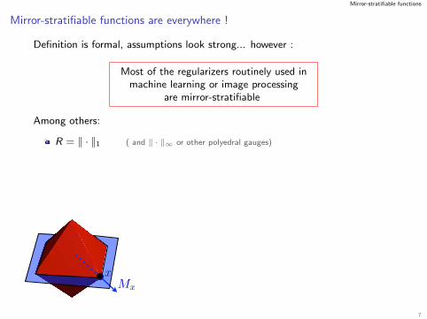
Mirror-stratifiable functions are everywhere !
Definition is formal, assumptions look strong... however :
Most of the regularizers routinely used inmachine learning or image processing
are mirror-stratifiable
Among others:
R = ‖ · ‖1 ( and ‖ · ‖∞ or other polyedral gauges)
nuclear norm (aka trace-norm) R(X ) =∑
i |σi (X )| = ‖σ(X )‖1
group-`1 R(x) =∑
b∈B ‖xb‖2 ( e.g. R(x) = |x1| + ‖x2,3‖ )
xMx
x Mx
x
Mx
7
Mirror-stratifiable functions
Mirror-stratifiable functions are everywhere !
Definition is formal, assumptions look strong... however :
Most of the regularizers routinely used inmachine learning or image processing
are mirror-stratifiable
Among others:
R = ‖ · ‖1 ( and ‖ · ‖∞ or other polyedral gauges)
nuclear norm (aka trace-norm) R(X ) =∑
i |σi (X )| = ‖σ(X )‖1
group-`1 R(x) =∑
b∈B ‖xb‖2 ( e.g. R(x) = |x1| + ‖x2,3‖ )
xMx
x Mx
x
Mx
7
Outline
1 Example in inverse problems (context and existing results)
2 Mirror-stratifiable functions
3 Optimization with mirror-stratifiable regularizersSensitivity under small variationsActivity identification of proximal algorithmsModel recovery in inverse problemsModel consistency in learning
4 Numerical illustrations
Optimization with mirror-stratifiable regularizers
Sensitivity of parametrized problems
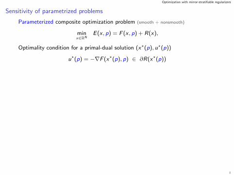
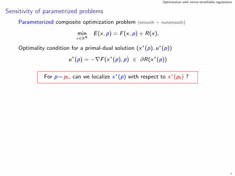
Parameterized composite optimization problem (smooth + nonsmooth)
minx∈RN
E(x , p) = F (x , p) + R(x),
Optimality condition for a primal-dual solution (x?(p), u?(p))
u?(p) = −∇F (x?(p), p) ∈ ∂R(x?(p))
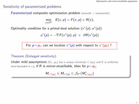
For p∼p0, can we localize x?(p) with respect to x?(p0) ?
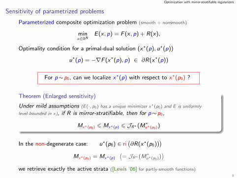
Theorem (Enlarged sensitivity)
Under mild assumptions (E(·, p0) has a unique minimizer x?(p0) and E is uniformly
level-bounded in x), if R is mirror-stratifiable, then for p∼p0,
Mx?(p0) 6 Mx?(p) 6 JR∗(M∗u?(p0))
In the non-degenerate case: u?(p0) ∈ ri(∂R(x?(p0))
)Mx?(p0) = Mx?(p)
(= JR∗(M∗u?(p0))
)we retrieve exactly the active strata ([Lewis ’06] for partly-smooth functions)
8
Optimization with mirror-stratifiable regularizers
Sensitivity of parametrized problems
Parameterized composite optimization problem (smooth + nonsmooth)
minx∈RN
E(x , p) = F (x , p) + R(x),
Optimality condition for a primal-dual solution (x?(p), u?(p))
u?(p) = −∇F (x?(p), p) ∈ ∂R(x?(p))
For p∼p0, can we localize x?(p) with respect to x?(p0) ?
Theorem (Enlarged sensitivity)
Under mild assumptions (E(·, p0) has a unique minimizer x?(p0) and E is uniformly
level-bounded in x), if R is mirror-stratifiable, then for p∼p0,
Mx?(p0) 6 Mx?(p) 6 JR∗(M∗u?(p0))
In the non-degenerate case: u?(p0) ∈ ri(∂R(x?(p0))
)Mx?(p0) = Mx?(p)
(= JR∗(M∗u?(p0))
)we retrieve exactly the active strata ([Lewis ’06] for partly-smooth functions)
8
Optimization with mirror-stratifiable regularizers
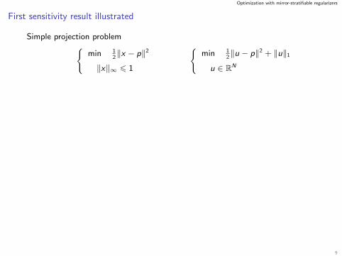
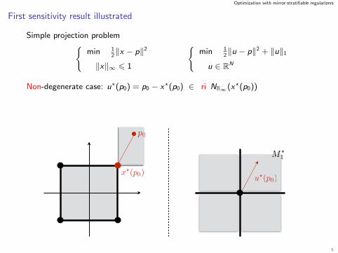
First sensitivity result illustrated
Simple projection problemmin 1
2‖x − p‖2
‖x‖∞ 6 1
min 1
2‖u − p‖2 + ‖u‖1
u ∈ RN
9
Optimization with mirror-stratifiable regularizers
First sensitivity result illustrated
Simple projection problemmin 1
2‖x − p‖2
‖x‖∞ 6 1
min 1
2‖u − p‖2 + ‖u‖1
u ∈ RN
Non-degenerate case: u?(p0) = p0 − x?(p0) ∈ ri NB∞(x?(p0))
x?(p0)
p0
u?(p0)
M1
9

Optimization with mirror-stratifiable regularizers
First sensitivity result illustrated
Simple projection problemmin 1
2‖x − p‖2
‖x‖∞ 6 1
min 1
2‖u − p‖2 + ‖u‖1
u ∈ RN
Non-degenerate case: u?(p0) = p0 − x?(p0) ∈ ri NB∞(x?(p0))
=⇒ M1 = Mx?(p0) = Mx?(p) (in this case x?(p) = x?(p0))
x?(p0)
p0
u?(p0)
M1
p
u?(p)
9
Optimization with mirror-stratifiable regularizers
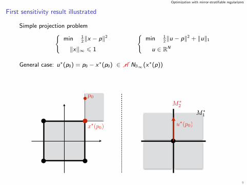
First sensitivity result illustrated
Simple projection problemmin 1
2‖x − p‖2
‖x‖∞ 6 1
min 1
2‖u − p‖2 + ‖u‖1
u ∈ RN
General case: u?(p0) = p0 − x?(p0) ∈ ri NB∞(x?(p))
x?(p0)
p0
u?(p0)
M1
M2
9

Optimization with mirror-stratifiable regularizers
First sensitivity result illustrated
Simple projection problemmin 1
2‖x − p‖2
‖x‖∞ 6 1
min 1
2‖u − p‖2 + ‖u‖1
u ∈ RN
General case: u?(p0) = p0 − x?(p0) ∈ ri NB∞(x?(p))
=⇒ M1 = Mx?(p0) 6 Mx?(p) 6 JR∗(M∗u?(p0)) = M2
x?(p0)
p0
u?(p0)
M1
M2
M2
9

Outline
1 Example in inverse problems (context and existing results)
2 Mirror-stratifiable functions
3 Optimization with mirror-stratifiable regularizersSensitivity under small variationsActivity identification of proximal algorithmsModel recovery in inverse problemsModel consistency in learning
4 Numerical illustrations
Optimization with mirror-stratifiable regularizers
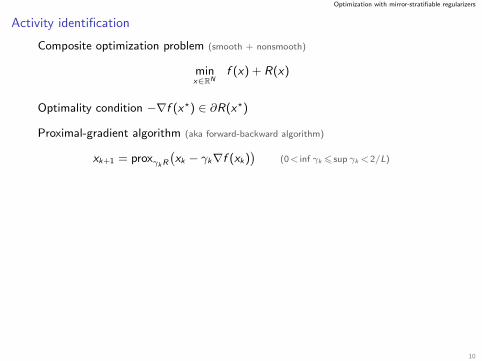
Activity identification
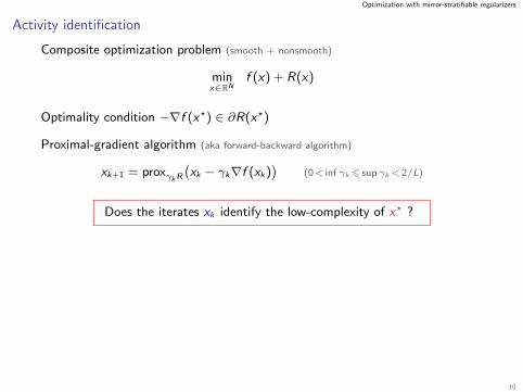
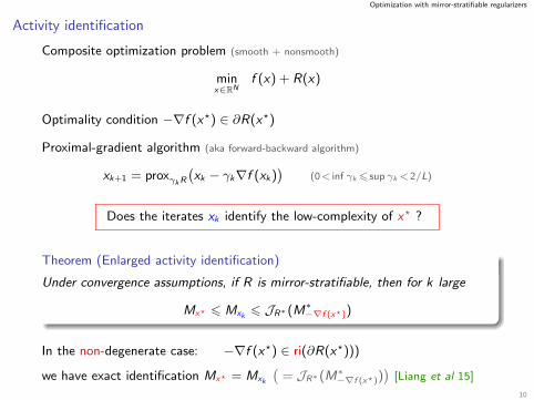
Composite optimization problem (smooth + nonsmooth)
minx∈RN
f (x) + R(x)
Optimality condition −∇f (x?) ∈ ∂R(x?)
Proximal-gradient algorithm (aka forward-backward algorithm)
xk+1 = proxγkR(xk − γk∇f (xk)
)(0< inf γk 6 sup γk<2/L)
Does the iterates xk identify the low-complexity of x? ?
Theorem (Enlarged activity identification)
Under convergence assumptions, if R is mirror-stratifiable, then for k large
Mx? 6 Mxk 6 JR∗(M∗−∇f (x?))
In the non-degenerate case: −∇f (x?) ∈ ri(∂R(x?)))
we have exact identification Mx? = Mxk
(= JR∗(M∗−∇f (x?))
)[Liang et al 15]
10
Optimization with mirror-stratifiable regularizers
Activity identification
Composite optimization problem (smooth + nonsmooth)
minx∈RN
f (x) + R(x)
Optimality condition −∇f (x?) ∈ ∂R(x?)
Proximal-gradient algorithm (aka forward-backward algorithm)
xk+1 = proxγkR(xk − γk∇f (xk)
)(0< inf γk 6 sup γk<2/L)
Does the iterates xk identify the low-complexity of x? ?
Theorem (Enlarged activity identification)
Under convergence assumptions, if R is mirror-stratifiable, then for k large
Mx? 6 Mxk 6 JR∗(M∗−∇f (x?))
In the non-degenerate case: −∇f (x?) ∈ ri(∂R(x?)))
we have exact identification Mx? = Mxk
(= JR∗(M∗−∇f (x?))
)[Liang et al 15]
10

Outline
1 Example in inverse problems (context and existing results)
2 Mirror-stratifiable functions
3 Optimization with mirror-stratifiable regularizersSensitivity under small variationsActivity identification of proximal algorithmsModel recovery in inverse problemsModel consistency in learning
4 Numerical illustrations
Optimization with mirror-stratifiable regularizers
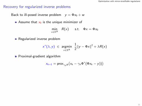
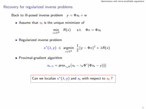
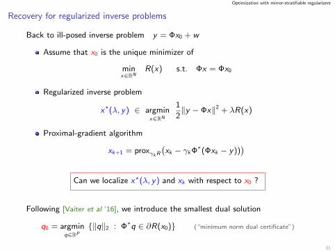
Recovery for regularized inverse problems
Back to ill-posed inverse problem y = Φx0 + w
Assume that x0 is the unique minimizer of
minx∈RN
R(x) s.t. Φx = Φx0
Regularized inverse problem
x?(λ, y) ∈ argminx∈RN
1
2‖y − Φx‖2 + λR(x)
Proximal-gradient algorithm
xk+1 = proxγkR(xk − γkΦ∗(Φxk − y))
)
Can we localize x?(λ, y) and xk with respect to x0 ?
Following [Vaiter et al ’16], we introduce the smallest dual solution
q0 = argminq∈RP
‖q‖2 : Φ∗q ∈ ∂R(x0) (“minimum norm dual certificate”)
11
Optimization with mirror-stratifiable regularizers
Recovery for regularized inverse problems
Back to ill-posed inverse problem y = Φx0 + w
Assume that x0 is the unique minimizer of
minx∈RN
R(x) s.t. Φx = Φx0
Regularized inverse problem
x?(λ, y) ∈ argminx∈RN
1
2‖y − Φx‖2 + λR(x)
Proximal-gradient algorithm
xk+1 = proxγkR(xk − γkΦ∗(Φxk − y))
)Can we localize x?(λ, y) and xk with respect to x0 ?
Following [Vaiter et al ’16], we introduce the smallest dual solution
q0 = argminq∈RP
‖q‖2 : Φ∗q ∈ ∂R(x0) (“minimum norm dual certificate”)
11
Optimization with mirror-stratifiable regularizers
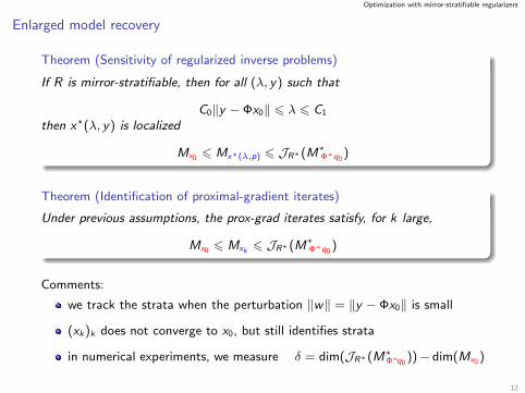
Enlarged model recovery
Theorem (Sensitivity of regularized inverse problems)
If R is mirror-stratifiable, then for all (λ, y) such that
C0‖y − Φx0‖ 6 λ 6 C1
then x?(λ, y) is localized
Mx0 6 Mx?(λ,p) 6 JR∗(M∗Φ∗q0)
Theorem (Identification of proximal-gradient iterates)
Under previous assumptions, the prox-grad iterates satisfy, for k large,
Mx0 6 Mxk 6 JR∗(M∗Φ∗q0)
Comments:
we track the strata when the perturbation ‖w‖ = ‖y − Φx0‖ is small
(xk)k does not converge to x0, but still identifies strata
in numerical experiments, we measure δ = dim(JR∗(M∗Φ∗q0))− dim(Mx0 )
12

Outline
1 Example in inverse problems (context and existing results)
2 Mirror-stratifiable functions
3 Optimization with mirror-stratifiable regularizersSensitivity under small variationsActivity identification of proximal algorithmsModel recovery in inverse problemsModel consistency in learning
4 Numerical illustrations
Optimization with mirror-stratifiable regularizers
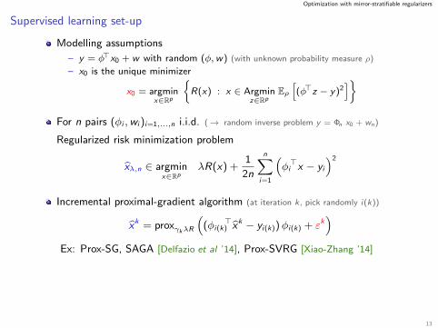
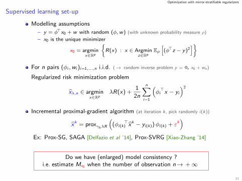
Supervised learning set-up
Modelling assumptions
– y = φ>x0 + w with random (φ,w) (with unknown probability measure ρ)
– x0 is the unique minimizer
x0 = argminx∈Rp
R(x) : x ∈ Argmin
z∈RpEρ[(φ>z − y)2
]For n pairs (φi ,wi )i=1,...,n i.i.d. (→ random inverse problem y = Φn x0 + wn)
Regularized risk minimization problem
xλ,n ∈ argminx∈Rp
λR(x) +1
2n
n∑i=1
(φi>x − yi
)2
Incremental proximal-gradient algorithm (at iteration k, pick randomly i(k))
xk = proxγkλR
((φi(k)
>xk − yi(k))φi(k) + εk)
Ex: Prox-SG, SAGA [Delfazio et al ’14], Prox-SVRG [Xiao-Zhang ’14]
Do we have (enlarged) model consistency ?i.e. estimate Mx0 when the number of observation n→ +∞
13
Optimization with mirror-stratifiable regularizers
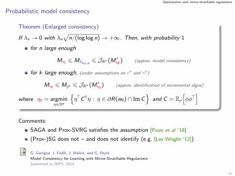
Probabilistic model consistency
Theorem (Enlarged consistency)
If λn → 0 with λn
√n/(log log n)→ +∞. Then, with probability 1
for n large enough
Mx0 6 Mxλn,n6 JR∗(M∗η0
) (approx. model consistency)
for k large enough, (under assumptions on εk and γk )
Mx0 6 Mzk 6 JR∗(M∗η0) (approx. identification of incremental algos)
where η0 = argminη∈Rp
η>C †η : η ∈ ∂R(w0) ∩ ImC
and C = Eρ
[φφ>
]
Comments:
SAGA and Prox-SVRG satisfies the assumption [Poon et al ’18]
(Prox-)SG does not – and does not identify (e.g. [Lee Wright ’12])
G. Garrigos, J. Fadili, J. Malick, and G. Peyre
Model Consistency for Learning with Mirror-Stratifiable Regularizers
Submitted to NIPS, 2018
14

Outline
1 Example in inverse problems (context and existing results)
2 Mirror-stratifiable functions
3 Optimization with mirror-stratifiable regularizersSensitivity under small variationsActivity identification of proximal algorithmsModel recovery in inverse problemsModel consistency in learning
4 Numerical illustrations
Numerical illustrations
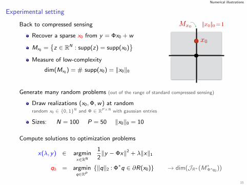
Experimental setting
Back to compressed sensing
Recover a sparse x0 from y = Φx0 + w
Mx0 =z ∈ RN : supp(z) = supp(x0)
Measure of low-complexity
dim(Mx0 ) = # supp(x0) = ‖x0‖0
x0
Mx0 ||x0||0 =1
Generate many random problems (out of the range of standard compressed sensing)
Draw realizations (x0,Φ,w) at randomrandom x0 ∈ 0, 1N and Φ ∈ RP×N with gaussian entries
Sizes: N = 100 P = 50 ‖x0‖0 = 10
Compute solutions to optimization problems
x(λ, y) ∈ argminx∈RN
1
2‖y − Φx‖2 + λ‖x‖1
q0 = argminq∈RP
‖q‖2 : Φ∗q ∈ ∂R(x0) → dim(JR∗(M∗Φ∗q0))
15
Numerical illustrations
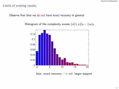
Limits of existing results
Observe first that we do not have exact recovery in general
Histogram of the complexity excess ‖x(λ, y)‖0 − ‖x0‖0
0 5 10 15 200
0.02
0.04
0.06
0.08
0.1
0.12
blue: exact recovery −→ red: larger support
16
Numerical illustrations
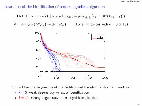
Illustration of the identification of proximal-gradient algorithm
Plot the evolution of ‖xk‖0 with xk+1 = proxγ‖·‖1
(xk − γΦ∗(Φxk − y))
)δ = dim(JR∗(M∗Φ∗q0
))− dim(Mx0 ) (For all instances with δ = 0 or 10)
δ quantifies the degeneracy of the problem and the identification of algorithm
δ = 0: weak degeneracy → exact identification
δ = 10: strong degeneracy → enlarged identification
17
Numerical illustrations
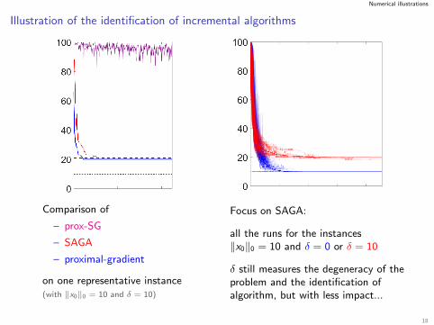
Illustration of the identification of incremental algorithms
Comparison of
– prox-SG
– SAGA
– proximal-gradient
on one representative instance(with ‖x0‖0 = 10 and δ = 10)
Focus on SAGA:
all the runs for the instances‖x0‖0 = 10 and δ = 0 or δ = 10
δ still measures the degeneracy of theproblem and the identification ofalgorithm, but with less impact...
18
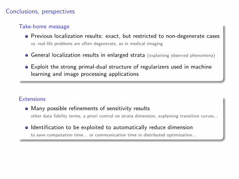
Conclusions, perspectives
Take-home message
Previous localization results: exact, but restricted to non-degenerate casesvs. real-life problems are often degenerate, as in medical imaging
General localization results in enlarged strata (explaining observed phenomena)
Exploit the strong primal-dual structure of regularizers used in machinelearning and image processing applications
Extensions
Many possible refinements of sensitivity resultsother data fidelity terms, a priori control on strata dimension, explaining transition curves...
Identification to be exploited to automatically reduce dimensionto save computation time... or communication time in distributed optimization...
thanks !!
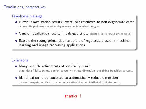