Embed Size (px)
Citation preview

J. Fluid Mech., page 1 of 24 c© Cambridge University Press 2010
doi:10.1017/S0022112009993764
1
Instability and sensitivity of the flow arounda rotating circular cylinder
JAN O. PRALITS1, LUCA BRANDT2†AND FLAVIO GIANNETTI1
1DIMEC, University of Salerno, Via Ponte don Melillo, 84084 Fisciano (SA), Italy2Linne Flow Centre, KTH Mechanics, S-100 44 Stockholm, Sweden
(Received 2 December 2008; revised 27 November 2009; accepted 3 December 2009)
The two-dimensional flow around a rotating circular cylinder is studied at Re = 100.The instability mechanisms for the first and second shedding modes are analysed. Theregion in the flow with a role of ‘wavemaker’ in the excitation of the global instability isidentified by considering the structural sensitivity of the unstable mode. This approachis compared with the analysis of the perturbation kinetic energy production, a classicapproach in linear stability analysis. Multiple steady-state solutions are found at highrotation rates, explaining the quenching of the second shedding mode. Turning pointsin phase space are associated with the movement of the flow stagnation point. Inaddition, a method to examine which structural variation of the base flow has thelargest impact on the instability features is proposed. This has relevant implicationsfor the passive control of instabilities. Finally, numerical simulations of the flow areperformed to verify that the structural sensitivity analysis is able to provide correctindications on where to position passive control devices, e.g. small obstacles, in orderto suppress the shedding modes.
1. IntroductionThe two-dimensional flow past a circular cylinder is one of the basic flow
configurations which have long received great attention from fluid dynamicists. Itis often used as a prototype to investigate vortex formation and the wake dynamicspast a bluff body. Less studied is the case of the flow past a rotating circular cylinder.Investigations of the latter flow have, in addition, implications for flow control usingwall motion owing to the reduced/increased relative velocity between body and freestream as well as the injection of additional momentum into the boundary layer. Inthe case of bodies of complex geometry, separate rotating circular cylinders can beused to control vortex shedding (see e.g. Modi 1997; Gad-El-Hak 2000).
As reviewed below, when increasing the rotational speed of the cylinder, twodistinct instability modes appear in the flow. The aim of this work is therefore toanalyse the instability mechanisms for the first and second shedding modes behind arotating circular cylinder. The region in the flow with a role of ‘wavemaker’ in theexcitation of the global instability is identified by considering the structural sensitivityof the unstable mode as introduced by Giannetti & Luchini (2007). This approach iscompared with the analysis of the perturbation kinetic energy production, a classic
† Email address for correspondence: [email protected]

2 J. O. Pralits, L. Brandt and F. Giannetti
approach in linear stability analysis (Drazin & Reid 1981; Huerre & Rossi 1998).Furthermore, we investigate which structural variation of the base flow has thelargest impact on the instability features. This may suggest how to control the vortexshedding by means of small obstacles or passive devices (see e.g. the experimentalwork by Strykowski & Sreenivasan 1990). From a stability point of view, the analysisperformed here extends the tools currently available for the analysis of complexflows. The need for global modes to account for spatially inhomogeneous flows isdiscussed for example by Theofilis (2003) and Chomaz (2005). Here, we show howthe combination of direct and adjoint global modes provides relevant knowledgeabout the structural sensitivity of the instability by identifying the core region for theinstability mechanism and the sensitivity to steady variations of the underlying baseflow, thus providing accurate indications for passive control strategies. For recentreviews on control of flow over a bluff body, the reader is referred to Collis et al.(2004) and Choi, Jeon & Kim (2008).
1.1. Sensitivity of instability modes to base-flow variations
A theoretical formulation for analysing the stabilization of wake flows by passivedevices was first proposed by Hill (1992), a work probably overlooked. Few yearslater, Bottaro, Corbett & Luchini (2003) examined the sensitivity of eigenvalues tomodifications of the base flow. The worst case, i.e. the change in base flow with themost destabilizing effect on the eigenvalues, is found using variational techniquesfor the plane Couette flow. Such base-flow variations are interpreted as differencesbetween the laboratory flow and its ideal, theoretical counterpart. Later studiesconsidered transition to turbulence initiated by base-flow defects (see e.g. Gavarini,Bottaro & Nieuwstadt 2004). Chomaz (2005) shows how small perturbations ofnon-normal operators may displace the eigenvalues in a significant manner. Theseperturbations will have a larger impact if they occur in the overlap region between theadjoint and direct global modes. Implications for feedback and closed-loop controlare also discussed; for each unstable mode, the influence of the control is limitedby its adjoint mode (see also Lauga & Bewley 2004). The analysis of structuralsensitivity of the instability past a cylinder by Giannetti & Luchini (2007) is extendedby Luchini, Giannetti & Pralits (2008, 2009). In the latter study, the effect of base-flowvariations on the limit cycle at supercritical Reynolds numbers and on the eigenvaluedrift is considered. These authors show that the sensitivity to base-flow modificationcan become significantly larger than that to perturbations. More recently, Marquet,Sipp & Jacquin (2008a) have developed sensitivity analyses that aim to predictvariations of the eigenvalue induced by arbitrary base-flow modifications. Theseauthors examine in particular the sensitivity to a steady force for the cylinder flowand obtain indications of the regions in the flow where base-flow modifications havea stabilizing effect. The results depend on the product of direct and adjoint modes.Marquet et al. (2008b) modelled the presence of a small control cylinder by a localforce and developed a multiple scale analysis to consider the sensitivity with respectto the steady and unsteady components of the force. This is, in other words, theforce acting on the unsteady shedding mode and on the steady base flow. FollowingLuchini et al. (2009), a very similar approach is used here for the case of a rotatingcylinder when considering the total flow sensitivity as the sum of the sensitivity toperturbations and base-flow modifications.
1.2. Flow past a rotating cylinder
Kang, Choi & Lee (1999) showed via numerical simulations that vortex sheddingbehind a rotating cylinder disappears when increasing the value of the ratio between

Instability of the flow around a rotating circular cylinder 3
the rotational velocity of the cylinder wall and the oncoming free stream α toabout 2. Furthermore, they observed that the rotation of the cylinder does notsignificantly alter the shedding frequency in the unstable range of rotation rates.Stojkovic, Breuer & Durst (2002) examined the flow at higher rotation rates andReynolds number Re =100, where the Reynolds number is based on the dimensionalfree-stream velocity U�
∞, the cylinder diameter D� and the kinematic viscosity ν�.These authors first documented the appearance of a second shedding mode in anarrow interval 4.85 � α � 5.15; this mode has a shedding frequency much lower thanthat of the classic von Karman vortex street (here also denoted by shedding mode I).Furthermore, the shedding period is dependent on the value of the rotation rate. Thequenching of shedding mode II was found to be associated with a kink in the curve forthe mean lift. A complete bifurcation diagram in the Reynolds-number-rotation-rateplane was provided by Stojkovic et al. (2003). The range of α where the second modeappears is only slightly decreasing when increasing the Reynolds number from 60 to200. At the same time, Mittal & Kumar (2003) performed simulations and stabilityanalysis for the flow at Re = 200. These authors also identify a second instabilitymode at α ≈ 4.5 and find two steady solutions of the nonlinear governing equationsfor large rotation rates. Note finally that only numerical studies are mentioned so far.Experimental measurements were performed by Barnes (2000) at low rotation rates todetermine the value at which shedding is suppressed for Reynolds numbers between50 and 65. The findings agree with the results of Kang et al. (1999). To the authors’knowledge, only one experimental work (Yildirim et al. 2008) reports a low-frequencyshedding at large rotation rates. The parameters in Yildirim et al. (2008) analysiswere Re =100 and α = 5.1.
Reynolds number Re = 100 is considered as by Stojkovic et al. (2002). While thelatter study is based on only direct numerical simulations (DNSs) of shedding modesI and II, stability and sensitivity analyses of the two modes are also presented here.In addition, numerical simulations of passive control are performed to validate thetheoretical predictions based on the flow sensitivity. Such a relatively low valuefor the Reynolds number is chosen to ensure the existence of two-dimensionalflow; the results obtained for larger values of the Reynolds number do not showsignificant differences in terms of instability mechanisms and sensitivity. A recentcomputational investigation by El Akoury et al. (2008) indicates that the cylinderrotation has a stabilizing effect on three-dimensional perturbations acting on sheddingmode I (α � 2.5), increasing thus the Reynolds number for two-dimensional/three-dimensional transition to values larger than those observed for the flow past anon-rotating cylinder (Re ≈ 190). On the other hand, the numerical simulations byMittal (2004) show the appearance of three-dimensional centrifugal instabilities atα = 5 and Re = 200. Therefore, the onset of three-dimensional flow past a rotatingcircular cylinder deserves further investigations.
2. Problem formulation and numerical methodThe two-dimensional flow past a rotating circular cylinder is considered here. As
mentioned above, two parameters completely define the present configuration: theReynolds number Re = (U�
∞D�)/ν� and the rotation rate α = ΩD�/2U�∞ with Ω being
the cylinder angular velocity. The dimensional free-stream velocity U�∞ and diameter
D� are used as reference velocity and length scales throughout the paper. The fluidmotion, in a domain D, is described by the two-dimensional unsteady incompressible

4 J. O. Pralits, L. Brandt and F. Giannetti
Navier–Stokes equations
∂U∂t
+ U · ∇U = −∇P +1
Re�U, (2.1)
∇ · U = 0, (2.2)
where U is the velocity vector with components U = (U, V ) and P is the reducedpressure. Equations (2.1) and (2.2) are given the following boundary conditions: onthe cylinder surface, the slip and no-penetration conditions are given by U · t =α andU · n = 0, respectively, where n and t are the normal and tangential versors to thesurface. In the far field, the flow approaches the incoming uniform stream, that isU → (U∞, 0) as r → ∞, where r is the distance from the cylinder centre.
2.1. Linear stability
The instability onset is studied using linear theory and a normal-mode analysis.The flow quantities are decomposed in a steady part and a small unsteadyperturbation as u(x, y, t) = Ub(x, y)+ εu(x, y, t) and P (x, y, t) = Pb(x, y)+ εp(x, y, t),where the amplitude ε is assumed to be small. Because we are interested in two-dimensional global modes, an ansatz is used such that u(x, y, t) = u(x, y) exp(σ t) andp(x, y, t) = p(x, y) exp(σ t). In the more general case in which one wishes to computethree-dimensional instability of a possibly time-periodic base flow, perturbations maybe expressed as u(x, y, z, t) = u(x, y, t) exp(σ t + γ z) where the homogeneity of thebase flow in the spanwise direction is accounted for by employing Fourier modes ofwavenumber γ and u(x, y, t) has the same periodicity of the base flow and imaginarypart of σ is the Floquet exponent. Introducing the flow decomposition and the ansatzinto (2.1) and (2.2) and linearizing, we obtain the linearized unsteady Navier–Stokesequations
σ u + L{Ub, Re}u + ∇p = 0, (2.3)
∇ · u = 0, (2.4)
where the base flow is the solution of the steady version of (2.1) and (2.2) and
L{Ub, Re}u = Ub · ∇u + u · ∇Ub − 1
Re�u. (2.5)
On the cylinder surface, a no-slip boundary condition is imposed while in the far fieldappropriate radiative boundary conditions should be used (see Giannetti & Luchini2007). At the outflow, a zero normal stress condition is imposed. At the upstreamboundary, the vorticity is set to zero while the streamwise velocity component isrequired to vanish (take the value of one for the Navier–Stokes equations (2.1) and2.2)) as 1/r , where r is the distance from the cylinder centre. Similarly, on the upperand lower boundaries, the normal velocity component v is assumed to decay as 1/r
and the vorticity is set to zero.The system (2.3) and (2.4) gives rise to a generalized eigenvalue problem for the
complex eigenvalue σ . For Re(σ ) < 0, the flow is stable while for Re(σ ) > 0, themode is unstable and grows exponentially in time.
2.2. Numerical method
The results presented here are obtained with the numerical code described byGiannetti & Luchini (2007). A second-order finite-difference approach is used tocompute spatial derivatives of the governing partial differential equations together

Instability of the flow around a rotating circular cylinder 5
with an immersed-boundary technique to represent the cylinder surface on a Cartesianmesh. The computational domain is rectangular.
With the spatial discretization and boundary conditions described above, threedifferent problems are addressed. First, the steady nonlinear Navier–Stokes equations(2.1) and (2.2) are solved by Newton iteration in order to compute the base flow usedfor the linear stability analysis. Arclength continuation, as explained by Keller (1977),is adopted for rotation rates above the onset of the second shedding mode wheremultiple steady-state solutions exist; see below. Second, the stability of the flow isinvestigated through the eigenvalue problem defined by the linearized perturbationequations (2.3) and (2.4), where an inverse iteration algorithm is implemented tocompute the least stable eigenvalue and eigenmode (see Giannetti & Luchini 2007 forfurther details on the numerical approach). Finally, the nonlinear Navier–Stokesequations are integrated forward in time with the hybrid Runge–Kutta/Crank–Nicholson scheme by Rai & Moin (1991) to verify the linear stability results andidentify the main features of the periodic flow arising in unstable configurations.
The main results are obtained with a computational domain of length Lx = 73 andLy = 54 in the streamwise x and cross-stream y directions, respectively. The cylinderis located symmetrically between the upper and lower boundaries, 25 diametersdownstream of the inflow. The Cartesian coordinate system has its origin in thecentre of the cylinder (xc = 0, yc = 0). The resolution used for most of the results is320 × 240 grid points in x and y. The results are validated by varying both resolutionand domain size. With a higher resolution of 480 × 360, the largest variation in themagnitude of the unstable eigenvalue is of about 0.8 %. When reducing the box sizeto Lx = 64 and Ly = 46, the relative error is of the order of 1.5 % for the largestrotation rates and much lower (0.2 %) for the lowest angular velocity examined. Asshown by Giannetti & Luchini (2007), an accurate estimate of the unstable eigenmodeis obtained when resolving the region of the wavemaker identified by flow structuralsensitivity in § 4.
3. Characteristics of the base flow and global mode3.1. Base flow
The flow past a non-rotating cylinder is symmetric and characterized by tworecirculation regions just behind the body (see e.g. Stojkovic et al. 2002). Whenincreasing the rotation rate of the cylinder, the lower of these two regions disappears(for counterclockwise rotation). The upper bubble, instead, detaches from the surfaceand becomes smaller (not shown here; cf. Stojkovic et al. 2002). The stagnation pointmoves away from the cylinder surface rotating in the direction opposite to that ofthe cylinder rotation. Further increasing the value of α, the upper vortex disappearsand flow is dominated by the rotation of the cylinder. The vorticity of the base flowfor rotation rates α = 1.8 and α = 4.85 is reported in figure 1. These values of α
correspond to the quenching of shedding mode I and to the onset of mode II. Thepositive and negative vorticities released in the lower and upper parts of the wake aredeflected upwards at the lower rotation rates considered, while they completely wraparound the cylinder for the largest α values under investigation.
Figure 2 displays the lift force acting on the rotating cylinder for all rotation ratesconsidered, α ∈ [0, 7]. In the figure, the stable and unstable solutions are indicatedwith dashed and solid lines, respectively, and the potential theory solution is shownwith a dotted line. As noted by Stojkovic et al. (2002), the behaviour at lower angularvelocities can be fitted by a quadratic relation. However, for values of the rotation

6 J. O. Pralits, L. Brandt and F. Giannetti
0 2 4 6 8 10
0
1
–1
–2
2
3(a)
(b)
0
5
–5
–10
10
0 2
0
–2
–1
1
2
3
0
–10
–20
10
20
Figure 1. Vorticity of base flow at rotation rate (a) α = 1.8 and (b) α = 4.85, Re =100.The white line depicts the evolution of the stagnation points for the steady solutionsreported in figure 2. The markers, starting from the cylinder surface, show the locationfor α = 2.5, 4, 4.85, 5.21, 5.17.
–25
–20
–15
–10
–5
0(a) (b)
0 1 2 3 4α α
5 6 7–14.75
–14.70
–14.65
–14.60
–14.55
–14.50
–14.45
–14.40
5.16 5.17 5.18 5.19 5.20 5.21 5.22
Fy
Figure 2. (a) Vertical force on the cylinder vs. rotation rate, Re = 100. Solid line denotesunstable nonlinear solution, and dashed line denotes stable base flow. The dotted line representsthe potential flow solutions. Note that positive rotation is counterclockwise and negative forceis downwards. (b) Details for the range of α where multiple solutions are found. The filledsquare and filled circle show the position of the two turning points.
rates larger than those at which the second shedding mode is observed, the increasein lift is almost proportional to α and its value approaches the results from potentialtheory. On the basis of early experimental work on flow past a rotating cylinder,Prandtl (1925) argued that the maximum lift that can be generated in a uniform flowis limited to 4π. The present results, in agreement with those of Mittal & Kumar(2003), show values of the lift coefficient exceeding the maximum limit based on thearguments by Prandtl. However, three-dimensional centrifugal instabilities, as wellas endwall and aspect-ratio effects, are expected to limit the lift generated via theMagnus effect. For a more detailed account on the issue, the reader is referred toChew, Cheng & Luo (1995), Mittal & Kumar (2003) and Mittal (2004) and referencestherein.
A close look at the region where the second shedding mode is found reveals theexistence of three different steady-state solutions of the governing equations (seeclose-up in figure 2). For a given α, the three steady-state solutions are very similarexcept for a small region in the vicinity of the stagnation point (therefore they arenot shown here). The base flow obtained at zero rotation cannot be continued for

Instability of the flow around a rotating circular cylinder 7
–0.02
0
0.02
0.04
0.06
0.08
0.10
0.12(a) (b)
5.16 5.17 5.18 5.19 5.20 5.21 5.22
σi
σr
α α
–0.02
0
0.02
0.04
0.06
0.08
0.10
0.12
5.16 5.17 5.18 5.19 5.20 5.21 5.22
Figure 3. (a) Frequency σi and (b) growth rate σr as a function of the rotation rate α. Thefilled square and the filled circle correspond to the left and right turning points in figure 2,respectively.
α > 5.21. The solution presents a turning point when represented in terms of the forceacting on the cylinder. A second turning point is observed at α ≈ 5.17. This locationdefines the upper limit at which the second shedding mode is observed and initiatesthe stable branch approaching the inviscid solution for increasing rotation rates. Thestability characteristics of the base flows depicted in figure 2 can be better explainedby the bifurcation diagram in terms of the rotation rate. Figure 3 shows both thefrequency σi and growth rate σr of the most unstable modes as a function of theparameter α. The left and right turning points in figure 2 are given by a filled squareand a filled circle, respectively. To interpret the bifurcation diagram, consider a pointmoving along the curve of figure 2 starting from α =5.17, where only one unstablecomplex mode exists (note that for the sake of clarity only positive frequencies areconsidered here; the spectrum is indeed symmetric with respect to the imaginary axis).If the rotation rate is increased, the frequency of the complex eigenvalue decreases tozero. This occurs at α ≈ 5.206, which is before the first turning point. At this α, twounstable modes appear, both pure real eigenvalues. Continuing along the curve, oneunstable solution becomes stable at the first turning point (filled circle). However, thesecond solution is still unstable, which explains why this turning point is not relatedto a change in the flow stability. The second solution becomes stable at the secondturning point (filled square); this is therefore the α giving the upper limit at whichthe second shedding mode is observed.
The kink observed in previous studies can thus be explained by the appearanceof multiple steady-state solutions of the Navier–Stokes equations at the values ofα where the second shedding mode cannot be seen any longer. The location of thestagnation point for the steady solutions computed here is presented in figure 1.The stagnation point is located above the cylinder, slightly downstream of its centre(xs, ys) = (0.17, 0.9), already for α = 4. However, the second shedding mode appearsonly when the stagnation points have moved sufficiently away from the cylindersurface, at (xs, ys) = (0.24, 1.84) for α = 4.85 and (xs, ys) = (0.11, 2.55) for α = 5.21.The loop in figure 2(b) is associated with a hook in the location of the stagnationpoint. It moves upstream and closer to the surface, (xs, ys) = (−0.025, 2.38) at α = 5.17above which shedding is not observed. Finally, the stable branch is associated witha stagnation point almost symmetrically above the cylinder and farther away forincreasing rotation rates.

8 J. O. Pralits, L. Brandt and F. Giannetti
6
5
4
3α
2
1
0 50 100Re
150 200
Mode IMode II
Mode I
Mode II
Figure 4. Neutral stability curve for the bi-dimensional flow past a rotating cylinder.
0 2 4 6
0
0.5
1.0
σ
α
Figure 5. Growth rates Re(σ ) (dashed line) and frequency Im(σ ) (solid line) vs. rotation rate,Re = 100. The symbols indicate the shedding frequency identified in the nonlinear simulationsof the flow (zero frequency for stable flow). The Strouhal number is related to the frequencyas St = Im(σ )/(2π).
3.2. Stability analysis
Linear stability analysis was performed in order to precisely calculate the neutralcurves for mode I and mode II in a Re–α plane. The results are reported in figure 4from which we easily observe the existence of two different unstable modes. Thesecond neutral point (higher α) for shedding mode II was obtained using arclengthcontinuation. Our results are in agreement with the numerical results of Stojkovicet al. (2003) obtained solving the nonlinear Navier–Stokes equations. However, thelinear stability and DNS results only agree in the vicinity of the neutral points, asalso shown by Mittal & Kumar (2003) for Re =200.
The growth rate and frequency of the most unstable modes pertaining to the baseflows presented in the previous section for Re = 100 are displayed in figure 5. Inthe plot, the frequency of the limit cycle as obtained from numerical simulations arealso reported with symbols. Positive real part of the eigenvalue, i.e. unstable flows,is found for 0 � α � 1.8, corresponding to the first shedding mode. The frequencyof the instability is increasing with the rotation rate. However, time integration ofthe nonlinear equations reveals that the shedding frequency is decreasing with α,as observed in previous studies (Mittal & Kumar 2003). Stable flow is found untilα = 4.85 when shedding mode II appears. As shown in the figure, this is characterized

Instability of the flow around a rotating circular cylinder 9
α DNS LST Stojkovic et al. (2002) Kang et al. (1999)
0 0.1646 0.1154 0.1650 –0.5 0.1647 0.1211 0.1657 –1 0.1656 0.1366 0.1658 0.16541.5 0.1634 0.1540 0.1626 –4.9 0.0294 0.0357 – –5 0.0226 0.0302 0.022 –5.1 0.0153 0.0229 – –
Table 1. Values of the Strouhal St = Im(σ )/(2π) as a function of the rotation rate α fordifferent investigations at Re = 100. DNS and LST denote the direct numerical simulationand linear stability analysis of the present work, respectively. The results from Stojkovic et al.(2002) and Kang et al. (1999) were obtained using DNS.
by frequencies significantly lower than those typical of the instability at low rotationrates. Numerical simulations confirm the presence of this low-frequency sheddingfor values of α where multiple solutions are not observed; cf. figure 2. Simulationsinitiated with an impulsive start converge to the stable solution for α > 5.17. At thesame time, solutions initiated with an instantaneous field from an unstable rotationrate become steady when increasing α above this threshold. Note that in the vicinityof the critical values of α, the shedding frequency observed in the flow matches thatobtained from the linear stability analysis, an indirect confirmation of the accuracyof the present results. Values of the Strouhal number St = Im(σ )/(2π) as a functionof the rotation rate α in comparison with other investigations are given in table 1.The values from both Stojkovic et al. (2002) and Kang et al. (1999) were obtainedfrom DNSs. The Strouhal numbers in the columns denoted by DNSs and LST (linearstability analysis) are from the present investigation. It can be seen that our DNSresults are in good agreement with those of both Stojkovic et al. (2002) and Kanget al. (1999).
The first instability mode at rotation rate α =1.8 and α = 4.85 is shown infigures 6(a) and 6(c), respectively. Shedding mode I is very similar to that observedfor α = 0. The shedding mode is deflected upward when compared with the case of norotation while the wake becomes narrower. Shedding mode II is instead associatedwith vorticity released from the upper part of the cylinder. Numerical simulationsof the governing nonlinear equations show that the instability occurs as sheddingof only one counterclockwise vortex. Positive vorticity is indeed accumulating closeto the stagnation point during large part of the shedding period (see also Mittal &Kumar 2003; Stojkovic et al. 2003).
The left or adjoint eigenvectors for shedding modes I and II are also displayed infigure 6. The adjoint field represents a sort of Green’s function for the receptivity ofthe corresponding global mode. The scalar product of the adjoint eigenmode withany forcing function and/or initial condition provides the amplitude of the instabilitymode (Chomaz 2005; Giannetti & Luchini 2007). Shedding mode I can thereforebe most efficiently triggered in the near wake of the cylinder, closer to the upperand lower sides and in the recirculation bubble farther downstream. The region ofmaximum receptivity for shedding mode II is located close to the body surface, inthe lower and rear part and is stronger than that of mode I. Weak sensitivity toforcing/initial conditions upstream of the cylinder is also observed.

10 J. O. Pralits, L. Brandt and F. Giannetti
0 5 10 15
0
2
–2 –2
–2
4
6
(a)
(c)(d)
(b)
0
5
–5
0
2
4
0
0.5
1.0
1.5
0 5 10 15
0
2
–2
4
6
0
2
–2
–4
–6
4
0 2–2–4
0 2–2–4
0
2
4
0
0.5
1.0
1.5
Figure 6. First instability mode and its adjoint at rotation rate (a,b) α = 1.8 and (c,d ) α = 4.85 ,Re = 100. (a,c) The real part of the vorticity of the unstable eigenmode and (b,d ) the magnitudeof the adjoint mode.
4. Structural sensitivity and the wavemakerIn this section, the sensitivity of the unstable shedding mode is used to identify
the core of the instability. The flow around a circular cylinder is often used as aprototype for globally unstable flows; these behave like hydrodynamic oscillators. Inweakly non-parallel flows, the Wentzel, Kramer, Brillioun, Jeffrey (WKBJ) approachenables us to identify a specific spatial position in the absolutely unstable regionwhich acts as a wavemaker, determining for example the oscillation frequency by thesaddle point criterion (Chomaz, Huerre & Redekopp 1991; Dizes et al. 1996; Chomaz2005). For more complex configurations, strong non-parallel effects prevent us fromusing the asymptotic theory and a global analysis is necessary. In this context, aconcept similar to that of wavemaker can be introduced by investigating where inspace a modification in the structure of the problem produces the largest drift of theeigenvalue: this is done by determining the region where feedback from velocity toforce is most effective. The derivation is briefly outlined here for continuous operatorsand further details are given by Giannetti & Luchini (2007).
We start by considering the perturbed eigenvalue problem satisfying the equations
σ ′u′ + L{Ub, Re}u′ + ∇p′ = δH(u′
, p′), (4.1)
∇ · u′ = 0, (4.2)
given homogeneous boundary conditions. The right-hand side δH denotes a lineardifferential operator expressing the structural perturbation of the original problem.In this paper, following Giannetti & Luchini (2007), we will consider structuralperturbation localized in space in the form of a local force proportional to a local

Instability of the flow around a rotating circular cylinder 11
velocity, i.e. we will assume
δH(u′, p
′) = δM(x, y) · u′ = δ(x − x0, y − y0) δM0 · u′, (4.3)
where δM0 is a 2 × 2 matrix of the coupling coefficients expressing the particular formof the localized structural perturbation and δ(x − x0, y − y0) stands for the Kroneckerdelta function.
The eigenvalue drift δσ and corresponding variation of the eigenfunctionsδq = {δu, δp} with respect to the unperturbed problem can be derived using theexpansion u′ = u + δu and p
′ = p + δp. If the expansion is inserted into (4.1) and (4.2)and quadratic terms are dropped, one easily obtains
σδu + L{Ub, Re}δu + ∇δp = −δσ u + δM · u, (4.4)
∇ · δu = 0. (4.5)
In order to derive an expression for the structural sensitivity, we now introducethe Lagrange identity, as in the work by Giannetti & Luchini (2007). The Lagrangeidentity is constructed for any pair of suitably differentiable fields q ≡ {u, p} andg+ ≡ { f +, m+}, which do not have to satisfy the linearized Navier–Stokes equations(2.3)–(2.4), using differentiation by parts
[ (σ u + L{Ub, Re}u + ∇p
)· f + + ∇·u m+
]
+
[u ·
(−σ f + + L+{Ub, Re} f + + ∇m+
)+ p ∇· f +
]= ∇· J(q, g+). (4.6)
In the above equation, J(q, g+) is the ‘bilinear concomitant’
J(q, g+) = Ub(u · f +) +1
Re
(∇ f + · u − ∇u · f +
)+ m+ u + p f +, (4.7)
and L+ is the adjoint linearized Navier–Stokes operator, which in vector notation canbe expressed as
L+{Ub, Re} f + = Ub · ∇ f + − ∇Ub · f + +1
Re� f +. (4.8)
The Lagrange identity is now applied to the perturbation field δq(x, y), satisfying
(4.4) and (4.5) and the adjoint field g+(x, y), where g+(x, y) = { f+, m+}. After
integrating over the domain D and accounting for the boundary conditions, wearrive at
−δσ
∫D
f + · u dS +
∫D
f + · δM · u dS =
∮∂D
J(q, g+) · n dl. (4.9)
Here the adjoint perturbation g+(x, y) = { f+, m+} satisfies the following
homogeneous equations
−σ f + + L+{Ub, Re} f + + ∇m+ = 0, (4.10)
∇ · f +b = 0, (4.11)

12 J. O. Pralits, L. Brandt and F. Giannetti
0
–1
–2–2 0 2
1
2
3
4(a) (b)
0
0.2
0.4
0.6
0.8
1.0
1.2
0
–1
–2–2 0 2
1
2
3
4
0
0.5
1.0
1.5
Figure 7. Structural sensitivity for shedding modes I and II at rotation rate (a) α = 1.8 and(b) α =4.85, Re = 100. Sensitivity with respect to perturbations.
and the boundary conditions are chosen such that the integral on the right-hand sideof (4.9) vanishes. Introducing the sensitivity tensor
S(x0, y0) =f +(x0, y0) u(x0, y0)∫
Df + · u dS
, (4.12)
we can express the eigenvalue drift due to the local feedback using (4.9) as
δσ (x0, y0) =
∫D
f + · δM · u dS∫D
f + · u dS
=f + · δM0 · u∫D
f + · u dS
=S : δM0 =∑
ij
Sij δM0ij . (4.13)
In the above expression, the notation f + u indicates the dyadic product between thedirect and adjoint modes.
Different norms of the tensor S can be used to build a spatial map of the sensitivity.The spectral norm is chosen here to study the worst possible case.
The structural sensitivity for shedding modes I and II at rotation rate α = 1.8 andα = 4.85, Re =100, are shown in figure 7. The core of the instability for sheddingmode I is found to be in two lobes placed asymmetrically in the near wake. One ofthe lobes is located across the separation bubble similar to the case of zero rotationrate (see Giannetti & Luchini 2007). An analysis of the perturbation kinetic energyproduction (see the next section) further suggests that the quenching of shedding modeI is promoted by the weakening of the upper recirculation bubble with increasingrotation rate α. The wavemaker of shedding mode II is, conversely, wrapped aroundthe cylinder, following the counterclockwise cylinder rotation.
4.1. Analysis of perturbation energy production
The instability mechanisms are often examined by considering the production of theperturbation kinetic energy. The basic idea is to derive in the usual way the equationgoverning the evolution of the perturbation kinetic energy density EV = 1/2uiui
from the governing linearized equations. Upon integration in the two-dimensionaldomain D, the divergence terms in the evolution equation give zero contributionto the global energy balance when the domain is assumed large enough to have

Instability of the flow around a rotating circular cylinder 13
0 5 10 15
0
–2
2
4
(a) (b)
0
0.2
–0.2
0.4
0.6
0 2 4
0
2
–2
–2
4
0
2
4
Figure 8. Density of the production of perturbation kinetic energy for shedding modes Iand II at rotation rate (a) α = 1.8 and (b) α =4.85, Re = 100.
negligible disturbances at the boundaries. Assuming the normal mode expansion forthe perturbation and averaging in time, the kinetic energy budget can be written as
d
dt
∫D
(1
2uiui
)dxi =
∫D
∂Ui
∂xj
τijdxi − 1
Re
∫D
ωiωidxi, (4.14)
where ( ) indicates time averages, ωi indicates the perturbation vorticity, Ui indicatesthe base-flow velocity and τij = − uiuj indicates the Reynolds stresses. The first termon the right-hand side is the production density, whereas the second term indicatesviscous dissipation (see e.g. Huerre & Rossi 1998).
The total production density (∂Ui/∂xj )τij is displayed in figure 8 for rotation ratesα = 1.8 and α = 4.85. For shedding mode I, production is largest a few diametersdownstream of the cylinder. For this instability, there is noteworthy difference betweenthe region of largest sensitivity (cf. figure 7) and that of largest disturbance generation.According to asymptotic theory, this can be explained by the fact that the wavemakeris located in a region of absolute instability in which the perturbations originateand propagate as waves in all directions. These waves are, however, most amplifiedfarther downstream, where the base flow is characterized by the strongest shear. Theperturbation kinetic energy production is almost entirely due to the shear ∂U/∂y;smaller positive contribution from Tyy = (∂V /∂y)τyy and negative from Txx is alsoobserved three diameters downstream of the cylinder at the end of the recirculationregion. The total production decreases by about 30 % when increasing the rotationrate from α =0 owing to the weakening of the shear layers associated with theseparated flow in the wake.
The perturbation kinetic energy production pertaining to shedding mode II is alsopresented in figure 8. First, one can note stronger peak values for the productionwhen compared with the case of shedding mode I. This also implies stronger vorticityand dissipation. The production is mainly due to the terms Tyx and Tyy , thus due tovariations of the velocity V of the base flow close to the stagnation point. A significantcontribution is also given by the production term associated with ∂U/∂y in the regionclose to the upper surface of the cylinder, where flow is moving towards the stagnationpoint. When comparing the energy production with the mode sensitivity (figure 7),good agreement is observed. For this instability, the two approaches pursued hereprovide a similar indication. However, if one wishes to influence the instability bymeans of a steady forcing, like a small obstacle placed in the flow field, a differentanalysis would be necessary. This is presented next.

14 J. O. Pralits, L. Brandt and F. Giannetti
5. Structural sensitivity to base-flow modificationsIn this section, an expression is derived for the eigenvalue drift δσ due to a
structural perturbation acting at the base-flow level. As in the previous sections,we will consider a structural perturbation of the steady nonlinear equations in theform of a local feedback from velocity to force. The perturbed base-flow solutionQb
′ = (Ub′, Pb
′) therefore depends on the particular choice of the coupling coefficientmatrix δM which characterizes the given feedback process. Because the eigenvalueσ is a function of the base flow, the functional relation between the eigenvalueand δM is easily expressed as σ = σ ( Qb
′(δM)). Recently, Marquet et al. (2008a)studied the sensitivity of the eigenvalue to structural perturbations of the base-flowequations using a Lagrange-multiplier technique. They first evaluated the sensitivityof the eigenvalue to a generic variation of the base flow and then used these resultsto determine the effect produced by a steady force, parallel to the local velocity,acting on the steady base-flow equations. Here, instead, we follow a slightly differentapproach based on the Lagrange identity. It is based on the method proposed byLuchini et al. (2008, 2009) in order to extend the theory of Giannetti & Luchini (2007)to a periodic base flow. In particular, we assume a general linear feedback acting onthe steady base-flow equations.
The derivation is made in two steps. We start by deriving an expression for theeigenvalue drift due to an arbitrary variation of the base flow in the linear stabilityproblem. Second, we demonstrate how to introduce a particular variation of the baseflow caused by the structural perturbation previously discussed.
The perturbed eigenvalue problem this time is given as
σδu + L{Ub, Re}δu + ∇δp = −[δσ u + δC(δUb, u)], (5.1)
∇ · δu = 0, (5.2)
where the bilinear operator δC,
δC(δUb, u) = δUb · ∇u + u · ∇δUb, (5.3)
expresses the variation of L due to a variation of the base flow δUb. We nowapply the same procedure as described in § 4. The Lagrange identity is applied tothe perturbation field δq(x, y, t) = δq(x, y) exp(σ t), satisfying (5.1) and (5.2) and theadjoint field g+(x, y, t) = g+(x, y) exp(−σ t). After integrating over the domain D andaccounting for the boundary conditions, we arrive at
δσ = −
∫D
f + · δC(δUb, u) dS∫D
f + · u dS
, (5.4)
which relates the eigenvalue drift to a variation of the base flow and the adjointperturbation field which satisfies (4.10) and (4.11). This expression can be expandedas
δσ =
∫D
δUb · δC+( f +, u) dS −∮
∂D(δUb · f +)u · n dl∫
Df + · u dS
, (5.5)
where the second integral in the numerator is obtained via integration by parts andvanishes if the solution decays at infinity. In this expression, the operator δC+, defined

Instability of the flow around a rotating circular cylinder 15
as
δC+( f +, u) = u · ∇ f + − ∇u · f +, (5.6)
is the adjoint of δC and corresponds to the sensitivity to a generic base-flowmodification as explained by Marquet et al. (2008a). The variation of the baseflow due to the structural perturbation is governed by the linearized steady base-flowequations
L{Ub, Re}δUb + ∇δPb = δM · Ub, (5.7)
∇ · δUb = 0. (5.8)
Using again the Lagrange identity on the base-flow field δ Qb(x, y) = {δUb, δPb}, whichsatisfies (5.7) and (5.8), and on the adjoint field G+
b (x, y) = { f +b , m+
b }, after integrationby part, we obtain an expression relating to the structural perturbation and thecorresponding variation of the base flow∫
DδUb · δC+( f +, u) dS = −
∫D
f +b · δM · Ub dS +
∮∂D
J(δ Qb, G+b ) · n dl, (5.9)
where J(δ Qb, G+b ) is the ‘bilinear concomitant’ defined in § 4. Here the adjoint base
flow G+b (x, y) = { f +
b , m+b } satisfies the following inhomogeneous equations:
L+{Ub, Re} f +b + ∇m+
b = δC+( f +, u), (5.10)
∇ · f +b = 0, (5.11)
where the adjoint Navier–Stokes operator L+{Ub, Re} is defined as
L+{Ub, Re} f +b = Ub · ∇ f +
b − ∇Ub · f +b +
1
ReΔ f +
b . (5.12)
The boundary conditions of (5.10) and (5.11) are chosen such that the last integralon the right-hand side of (5.9) vanishes. Using (5.5) and (5.9), the eigenvalue drift canfinally be expressed as
δσ (x0, y0) =
∫D
f +b · δM · Ub dS∫
Df + · u dS
=f +
b (x0, y0) · δM0 · Ub(x0, y0)∫D
f + · u dS
= Sb(x0, y0) : δM0,
(5.13)where
Sb(x0, y0) =f +
b (x0, y0) Ub(x0, y0)∫D
f + · u dS
. (5.14)
Similar to the case of the structural sensitivity to perturbations, when the feedbackforcing is assumed to be localized in space, the sensitivity can be represented by aspatial map given by the dyadic product in (5.14). The structural sensitivity presentedin § 4 assumes a local force proportional to the local perturbation velocity, that isa time-periodic forcing with the frequency of the instability mode. Conversely, thesensitivity considered here assumes a local force proportional to the local base-flowvelocity, that is a steady forcing inducing small base-flow deformations.
The structural sensitivity pertaining to the flow around a cylinder rotating atα = 1.8 and α = 4.85 is shown in figure 9. For both cases, the sensitivity to base-flow modifications is significantly stronger than that to perturbations (see figure 7).The largest sensitivity is attained just below the cylinder, where the velocity at the

16 J. O. Pralits, L. Brandt and F. Giannetti
0 2 4
0
–1
–2–4 –2 0 2 4–4 –2
1
2
3
4
5
(a) (b)
0
1
2
3
4
0
1
–1
–2
2
3
4
5
0
5
10
15
Figure 9. Structural sensitivity for shedding modes I and II at rotation rate (a) α = 1.8 and(b) α = 4.85, Re = 100. Sensitivity with respect to variations of the base flow.
surface has the same direction of the free stream (the cylinder is rotating in thecounterclockwise direction). The most effective forcing is acting in such a way as tochange the apparent peripheral cylinder velocity and thus change the location of theflow stagnation point. As shown by the analysis of the base flows, small differencesin its location can have a significant effect on the stability characteristics. In addition,for mode II, this region in the flow corresponds also to the origin of the positive base-flow vorticity accumulating just above the cylinder before the shedding. For sheddingmode I, a region of relevant sensitivity associated with the two lobes identified asinstability cores is also shown. This suggests that a steady forcing in the region ofthe wavemaker can be effective. In the next section, the operator of the structuralperturbation will be defined so as to reproduce the effect of a small steady cylinderplaced in the vicinity of the rotating cylinder. In this case, the sensitivity of the modegrowth rate and shedding frequency will be considered separately.
6. Application to passive controlWe will now use the previous results to develop an effective passive control strategy
for the flow around a rotating cylinder. In principle, several different approaches canbe used to control the flow behind a bluff body. A very simple one was suggested byStrykowski & Sreenivasan (1990), who introduced a small control cylinder in the wakeof the main one. They noted that by choosing a proper placement of the secondarycylinder, the vortex shedding was considerably altered and even suppressed altogetherover a limited range of Reynolds numbers. Temporal growth rate measurements ofthe velocity fluctuations revealed that the presence of the smaller cylinder reduces thegrowth rate of the disturbances leading to vortex shedding and that its suppression,accompanied by the disappearance of sharp spectral peaks, coincides with negativetemporal growth rates. Here we will adopt the control strategy proposed by Strykowski& Sreenivasan (1990) to the case of the rotating cylinder and present results formode II.
The effects of a small control cylinder on the flow field can be studied in terms of thestructural sensitivity analysis previously set forth. The placement of a small cylinder ofdiameter d� in the near wake of a bluff body, in fact, results in a reaction force actingon the fluid which modifies the flow field and leads to a shift of the eigenvalue σ .Because the control cylinder is small, its presence can be thought of as a localizedstructural perturbation of the governing equations consisting in a localized feedback

Instability of the flow around a rotating circular cylinder 17
from velocity to force. In the limit of an infinitely small control cylinder placed at(x0, y0), the local reacting force can be modelled by the first term of the Lamb–Oseenexpansion for the drag of a cylinder in a creeping flow (see e.g. Pozrikidis 1996; Dyke1975). With our non-dimensionalization, the expression for the reacting force becomes
F(x, y) ≈ −δA δ(x − x0, y − y0) U(x, y), (6.1)
where the real coefficient δA is given by the following formula
δA =4π
Re ln
(7.4
Rec
) . (6.2)
Note that δA depends on the usual Reynolds number of the flow under investigationand on the Reynolds number of the small control cylinder Rec = U�d�/ν� which isbased on its diameter and on the local velocity U(x0, y0). As expected, δA → 0 asRec → 0 (i.e. d� → 0) so that, in this limit, the effects of the reacting force canbe investigated through the linear structural perturbation analysis developed in theprevious sections. Equation (6.1) represents a force of pure resistance, i.e. a forcewhose direction is locally aligned with the local velocity vector. This means that thelocal feedback matrix δM0 corresponding to (6.1) is diagonal with elements of equalmagnitude δA, i.e. δM0 = δA I (with I being the identity 2 × 2 matrix). The structuralperturbation acts both at the perturbation level by modifying in a direct way thestructure of the eigenvalue problem and at the base-flow level by perturbing the steadybase flow, which in turn determines the coefficients of the linearized Navier–Stokesoperator. In order to build a spatial map which can be used as a guideline for acontrol strategy, both effects must be taken into consideration. Therefore, given theparticular form of the structural perturbation, we can write the total eigenvalue driftδσt as the sum of the two contributions
δσt = δσb + δσ = Sb : δM0 + S : δM0 = St : δM0, (6.3)
where the total sensitivity is defined as
St = S + Sb. (6.4)
It is important to note that by inspecting the real and imaginary part of (6.3), it ispossible to uncover the effect of the structural perturbation on the growth rate andthe frequency of the unstable mode, respectively.
This formula is valid only for an infinitesimal perturbation, i.e. for infinitesimalsmall control cylinders. Marquet et al. (2008a) used a different formula numericallycalibrated to model the effect of a small but finite cylinder. With such formula andaccounting only for the sensitivity to the base-flow modification, they obtained goodagreement with the experimental results of Strykowski & Sreenivasan (1990). Here,we prefer to build the sensitivity map for an infinitely small control cylinder with(6.3) and use it only as a guide to place a control device of small but finite radius inthe flow field. The real effects of such positioning will be then checked by runninga full DNS for the flow over the two cylinders. This will enable us to comparethe results with our sensitivity map and to check that no other stable modes aredestabilized by the present control strategy. This is an essential point: indeed for thesuccess of any control strategy, the sensitivity of the dominant stable modes shouldalso be examined. However, given the level of approximation used to represent thesecondary cylinder, we think it is more convenient to directly perform the DNS, which

18 J. O. Pralits, L. Brandt and F. Giannetti
0 2
0
–1
–2
–1
–2
–1
–2
–1
–2
–3
–1
–2
–3
–2
–2
1δσ
δσb
δσt
2
3
4(a) (b)
0
0.5
–0.5
–1.0
1.0
0 2
0
1
–1
–2
–1
–2
–1
–2
–1
–2
–3
–1
–2
–3
–2
–2
–2
2
3
4
0
0.5
–0.5
–1.0
1.0
0 2
–2 0 2
0
1
2
3
4
0
1
2
3
0 2
0
1
2
3
4
0
1
2
3
0
1
2
3
4
0
1
2
3
0 2
0
1
2
3
4
0
1
2
3
Figure 10. Structural sensitivity for shedding mode I at rotation rate α = 1.8. (a) Realpart with negative value indicating quenching and (b) imaginary part with negative valueindicating lowering of the shedding frequency. From top to bottom, sensitivity with respect toperturbations δσ , to variations of the base flow δσb and total sensitivity δσt .
also includes nonlinear effects neglected in the sensitivity analysis. This will thereforeprovide a good validation of the theoretical model.
6.1. Sensitivity map for the shedding modes
In figures 10 and 11, the variations δσ , δσb and δσt (from top to bottom) are shownfor a structural perturbation of amplitude δA = 1 for shedding mode I (Re = 100,α = 1.8) and II (Re = 100, α = 5.0), respectively. In principle, keeping δA constant for

Instability of the flow around a rotating circular cylinder 19
0 2
0
–1
–2
–1
–2
–1
–2
–5
–10
–2
–2
1δσ
δσb
δσt
2
3
4(a) (b)
0
0.5
–0.5
–1.0
1.0
0 2
0
1
–1
–2
–1
–2
–1
–2
–2
–2
–2
2
3
4
0
0.5
–0.5
–1.0
1.0
0 2
–2 0 2
0
1
2
3
4
0
5
10
–5
–10
0
5
10
–5
–10
0
5
10
–10
–20
0
10
20
0 2
0
1
2
3
4
0
1
2
3
4
0 2
0
1
2
3
4
Figure 11. Structural sensitivity for shedding mode II at rotation rate α = 5. (a) Realpart with negative value indicating quenching and (b) imaginary part with negative valueindicating lowering of the shedding frequency. From top to bottom, sensitivity with respect toperturbations δσ , to variations of the base flow δσb and total sensitivity δσt .
different positions of the control cylinder implies considering different diameters d∗.However, in the range of validity of our sensitivity analysis (d∗ → 0), the dependenceof the amplitude on the local Reynolds number can be considered a second-ordereffect. The variation, of each quantity, with respect to the growth rate is shown infigure 10(a), where a negative value indicates quenching. Figure 10(b), instead, showsthe variation with respect to the shedding frequency with dark areas corresponding tolowering. In both cases, variations due to base-flow modifications are larger than the
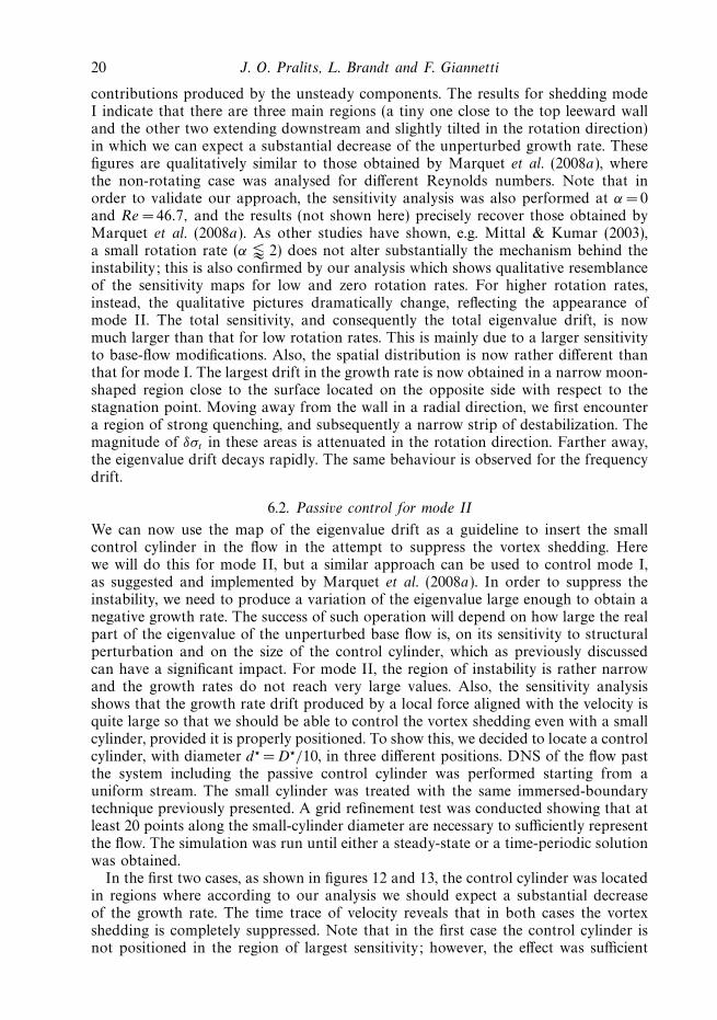
20 J. O. Pralits, L. Brandt and F. Giannetti
contributions produced by the unsteady components. The results for shedding modeI indicate that there are three main regions (a tiny one close to the top leeward walland the other two extending downstream and slightly tilted in the rotation direction)in which we can expect a substantial decrease of the unperturbed growth rate. Thesefigures are qualitatively similar to those obtained by Marquet et al. (2008a), wherethe non-rotating case was analysed for different Reynolds numbers. Note that inorder to validate our approach, the sensitivity analysis was also performed at α = 0and Re = 46.7, and the results (not shown here) precisely recover those obtained byMarquet et al. (2008a). As other studies have shown, e.g. Mittal & Kumar (2003),a small rotation rate (α � 2) does not alter substantially the mechanism behind theinstability; this is also confirmed by our analysis which shows qualitative resemblanceof the sensitivity maps for low and zero rotation rates. For higher rotation rates,instead, the qualitative pictures dramatically change, reflecting the appearance ofmode II. The total sensitivity, and consequently the total eigenvalue drift, is nowmuch larger than that for low rotation rates. This is mainly due to a larger sensitivityto base-flow modifications. Also, the spatial distribution is now rather different thanthat for mode I. The largest drift in the growth rate is now obtained in a narrow moon-shaped region close to the surface located on the opposite side with respect to thestagnation point. Moving away from the wall in a radial direction, we first encountera region of strong quenching, and subsequently a narrow strip of destabilization. Themagnitude of δσt in these areas is attenuated in the rotation direction. Farther away,the eigenvalue drift decays rapidly. The same behaviour is observed for the frequencydrift.
6.2. Passive control for mode II
We can now use the map of the eigenvalue drift as a guideline to insert the smallcontrol cylinder in the flow in the attempt to suppress the vortex shedding. Herewe will do this for mode II, but a similar approach can be used to control mode I,as suggested and implemented by Marquet et al. (2008a). In order to suppress theinstability, we need to produce a variation of the eigenvalue large enough to obtain anegative growth rate. The success of such operation will depend on how large the realpart of the eigenvalue of the unperturbed base flow is, on its sensitivity to structuralperturbation and on the size of the control cylinder, which as previously discussedcan have a significant impact. For mode II, the region of instability is rather narrowand the growth rates do not reach very large values. Also, the sensitivity analysisshows that the growth rate drift produced by a local force aligned with the velocity isquite large so that we should be able to control the vortex shedding even with a smallcylinder, provided it is properly positioned. To show this, we decided to locate a controlcylinder, with diameter d� =D�/10, in three different positions. DNS of the flow pastthe system including the passive control cylinder was performed starting from auniform stream. The small cylinder was treated with the same immersed-boundarytechnique previously presented. A grid refinement test was conducted showing that atleast 20 points along the small-cylinder diameter are necessary to sufficiently representthe flow. The simulation was run until either a steady-state or a time-periodic solutionwas obtained.
In the first two cases, as shown in figures 12 and 13, the control cylinder was locatedin regions where according to our analysis we should expect a substantial decreaseof the growth rate. The time trace of velocity reveals that in both cases the vortexshedding is completely suppressed. Note that in the first case the control cylinder isnot positioned in the region of largest sensitivity; however, the effect was sufficient

Instability of the flow around a rotating circular cylinder 21
0.85
0.90
0.95
1.00
1.05
1.10
1.15
1.20
1.25
1.30(b)
0 1001.00.50x
–0.5–1.0–1.0
–0.5
0.5
1.0(a)
0y
200 300 400 500
tu(
x p, y p
, t)
Figure 12. Control of vortex shedding, case 1. (a) Position of the control cylinder with respectto the variation of the growth rate. Dark colours indicate quenching and light colours indicatean increase. The area delimited by the solid contour is associated with δσt � 1.5, while thearea inside the dashed-dotted line contour is associated with δσt � −1.5. (b) Time trace of thestreamwise velocity component at the point xp =17, yp = 2 downstream of the main cylinder.The Strouhal number for the case without the control St =0.0226.
–0.8–1.0
–0.6–0.4–0.2
00.20.40.60.81.0
(b)
0 5001.00.50x
–0.5–1.0–1.0
–0.5
0.5
1.0(a)
0y
1000 1500 2000t
u(x p
, y p
, t)
Figure 13. Control of vortex shedding, case 1. (a) Position of the control cylinder with respectto the variation of the growth rate. Dark colours indicate quenching and light colours indicatean increase. The area delimited by the solid contour is associated with δσt � 1.5, while thearea inside the dashed-dotted line contour is associated with δσt � −1.5. (b) Time trace of thestreamwise velocity component at the point xp =17, yp = 2 downstream of the main cylinder.The Strouhal number for the case without the control St =0.0226.
to successfully control the instability. In addition, the transient regime to the steadystate is also shorter than that in the case when the control cylinder is placed in theregion of strongest sensitivity (figure 13).
Finally, in order to confirm the sensitivity map, a third test case, shown in figure 14,was examined. The control cylinder was placed in an area where an increase of thegrowth rate and a decrease of the shedding frequency are expected. In this case, theflow reached a periodic state with a lower frequency with respect to the unperturbedcase. This is in agreement with the results of figure 11.
7. ConclusionsThe linear instability of the flow around a rotating circular cylinder is studied at
Re =100. Structural sensitivity (Giannetti & Luchini 2007) and perturbation kineticenergy budget are considered to examine the relevant physical mechanisms for theinstability. The main conclusions can be summarized as follows.

22 J. O. Pralits, L. Brandt and F. Giannetti
0.2
0
0.4
0.6
0.8
1.0
1.2
1.4(b)
1001.00.50x
–0.5–1.0–1.0
–0.5
0.5
1.0(a)
0y
200 300 400 500t
u(x p
, y p
, t)
Figure 14. Control of vortex shedding, case 2. (a) Position of the control cylinder with respectto the variation of the growth rate. Dark colours indicate quenching and light colours indicatean increase. The area delimited by the solid contour is associated with δσt � 1.5, while thearea inside the dashed-dotted line contour is associated with δσt � −1.5. (b) Time trace ofthe streamwise velocity component at the point xp = 17, yp = 2 downstream of the maincylinder. The Strouhal numbers for the cases with and without the control are St = 0.0141and St = 0.0226, respectively.
The von Karman vortex street disappears when the rotation rate of the cylinderincreases to α ≈ 2. This is due to the weakening of the shear layers associated withflow in the wake. For this instability mode, the structural sensitivity identifies thewavemaker in the excitation of the global oscillations in the near wake region, whilethe largest production is observed farther downstream in the regions of strongestcross-stream shear. This difference motivates the need for different approaches to theglobal stability problem.
A second shedding mode is observed in the range 4.85 � α � 5.17, characterizedby the shedding of one counterclockwise vortex from the upper part of the cylinder.The core of the instability is identified in the advection of the positive vorticity ofthe base flow from the low–rear part of the cylinder to the stagnation point where itaccumulates and is then shed.
Multiple solutions are found at high rotation rates. Following the unstable branch,a first turning point in phase space is observed. For a limited range of α, two unstablebranches are thus found. The location of a second turning point determines therotation rate at which shedding mode II is last observed. In fact, this point definesthe birth of a branch with stable steady-state solutions, which continues at larger α.An analysis of these multiple steady states is presented for the first time. Turningpoints are associated with the movement of the flow stagnation point. This is, in turn,associated with the instability. Increasing the cylinder angular velocity, the stagnationpoint moves away from the cylinder rotating in the opposite direction. Sheddingmode II is observed when this is sufficiently far from the cylinder, so that positivevorticity can accumulate there, as well as downstream of the cylinder centre. Theinstability disappears once the point moves back upstream, while reaching fartherout for very high rotation rates approaching the potential flow solution. The flowtherefore transitions from an unstable regime where viscous effects are important toa stable configuration where rotation dominates. In this case, vorticity is not diffusedsufficiently far from the cylinder surface in the stagnation region and the flow is againstable.
A method to examine which structural variation of the base flow has the largestimpact on the instability features is proposed. This involves the product of the direct

Instability of the flow around a rotating circular cylinder 23
and adjoint modes weighted by the Jacobian of the linear stability system and ofthe steady Navier–Stokes equations subject to a steady structural perturbation. Themethod proposed has relevant implications for the control of instabilities. Whenapplied to the flow past a rotating cylinder, it provides for example indication onthe way to control the vortex shedding by placing an obstacle in the flow, as in theexperimental work by Strykowski & Sreenivasan (1990). Numerical simulations ofpassive control by means of a small non-rotating cylinder are performed to validatethe theoretical model adopted. A secondary cylinder is placed close to the mainrotating cylinder as suggested by the sensitivity map computed above. Quenching ofshedding mode II and variations of the shedding frequency are found in agreementwith the theoretical predictions.
Finally, a comment on the question of three-dimensional effects is in order. TheReynolds number pertaining to the computations presented here is chosen to be largeenough for the first bifurcation to occur (Re > 47) but lower than that when three-dimensional breakdown of the two-dimensional shedding is observed for the non-rotating cylinder (Re ≈ 190). For rotating cylinders, the investigation by El Akouryet al. (2008) indicates that the cylinder rotation has a stabilizing effect on three-dimensional perturbations acting on shedding mode I (α � 2.5), increasing thus theReynolds number for two-dimensional/three-dimensional transition to values largerthan those observed for the flow past a non-rotating cylinder. However, when furtherincreasing the rotation speed, the stagnation point moves away from the surfaceof the cylinder, and closed streamlines will form, separating the flow in internaland external to it. Within the internal flow, one can expect that the large pressuredifferences will induce three-dimensional centrifugal instabilities similar to that inTaylor–Couette flow. Indeed, the numerical simulations by Mittal (2004) of the flowpast a cylinder of finite spanwise length show the appearance of three-dimensionalcentrifugal instabilities at α = 5 and Re = 200. Further investigations are thereforeneeded on the onset of three-dimensional flow past a rotating circular cylinder.Floquet analysis needs to be performed when considering the instability of time-periodic base flows; extension of the structural sensitivity concept for this case ispresented by Luchini et al. (2008, 2009). Recent experimental work by Yildirim et al.(2008) reports low-frequency shedding at Re = 100 and α = 5.1.
The authors wish to thank Paolo Luchini and Simone Camarri for many fruitfuldiscussions. L. B. acknowledges financial support from the Goran GustafssonFoundation during his visit to Salerno.
REFERENCES
Barnes, F. H. 2000 Vortex shedding in the wake of a rotating circular cylinder at low Reynoldsnumbers. J. Phys. D. Appl. Phys. 33, L141–L144.
Bottaro, A., Corbett, P. & Luchini, P. 2003 The effect of base flow variation on flow stability.J. Fluid Mech. 476, 293–302.
Chew, Y. T., Cheng, M. & Luo, S. C. 1995 A numerical study of flow past a rotating circularcylinder using a hybrid vortex scheme. J. Fluid Mech. 299, 35–71.
Choi, H., Jeon, W.-P. & Kim, J. 2008 Control of flow over a bluff body. Annu. Rev. Fluid Mech. 40,113–139.
Chomaz, J.-M. 2005 Global instabilities in spatially developing flows: non-normality andnonlinearity. Annu. Rev. Fluid Mech. 37, 357–392.
Chomaz, J. M., Huerre, P. & Redekopp, L. G. 1991 A frequency selection criterion in spatiallydeveloping flows. Stud. Appl. Math. 84, 119–144.

24 J. O. Pralits, L. Brandt and F. Giannetti
Collis, S. S., Joslin, R. D., Seifert, A. & Theofilis, V. 2004 Issues in active flow control: theory,control, simulation, and experiment. Prog. Aerosp. Sci. 40, 237–289.
Dizes, S. L., Huerre, P., Chomaz, J. & Monkewitz, P. 1996 Linear global modes in spatiallydeveloping media. Phil. Trans. R. Soc. Lond. A 354 (1705), 169–212.
Drazin, P. & Reid, W. 1981 Hydrodynamic Stability . Cambridge University Press.
Dyke, M. V. 1975 Perturbation Methods in Fluid Mechanics . Parabolic Press.
El Akoury, R., Braza, M., Perrin, R., Harran, G. & Hoarau, Y. 2008 The three-dimensionaltransition in the flow around a rotating cylinder. J. Fluid Mech. 607, 1–11.
Gad-El-Hak, M. 2000 Flow Control: Passive, Active and Reactive Flow Management . CambridgeUniversity Press.
Gavarini, I., Bottaro, A. & Nieuwstadt, F. T. M. 2004 The initial stage of transition in pipe flow:role of optimal base-flow distortions. J. Fluid Mech. 517, 131–165.
Giannetti, F. & Luchini, P. 2007 Structural sensitivity of the first instability of the cylinder wake.J. Fluid Mech. 581, 167–197.
Hill, D. C. 1992 A theoretical approach for analysing the restablisation of wakes. AIAA Paper92-0067.
Huerre, P. & Rossi, M. 1998 Hydrodynamic instabilities in open flows. In Hydrodynamic andNonlinear Instabilities (ed. C. Godreche & P. Manneville), pp. 81–294. Cambridge UniversityPress.
Kang, S., Choi, H. & Lee, S. 1999 Laminar flow past a rotating circular cylinder. Phys. Fluids11 (11), 3312.
Keller, H. B. 1977 Numerical solution of bifurcation and nonlinear eigenvalue problems. InApplication of Bifurcation Theory, pp. 358–384. Academic Press.
Lauga, E. & Bewley, T. R. 2004 Performance of a linear robust control strategy on a nonlinearmodel of spatially developing flows. J. Fluid Mech. 512, 343–374.
Luchini, P., Giannetti, F. & Pralits, J. O. 2008 Structural sensitivity of linear and nonlinearglobal modes. In Proceedings of Fifth AIAA Theoretical Fluid Mechanics Conference, Seattle,Washington. AIAA Paper 2008-4227.
Luchini, P., Giannetti, F. & Pralits, J. O. 2009 Structural sensitivity of the finite-amplitude vortexshedding behind a circular cylinder. In IUTAM Symp. on Unsteady Separated Flows and TheirControl, 18–22 June 2007, Corfu, Greece, vol. 14, pp. 151–160. Springer.
Marquet, O., Sipp, D. & Jacquin, L. 2008a Sensitivity analysis and passive control of cylinderflow. J. Fluid Mech. 615, 221–252.
Marquet, O., Sipp, D., Jacquin, L. & Chomaz, J.-M. 2008b Multiple scale and sensitivity analysisfor the passive control of the cylinder flow. In Proceedings of Fifth AIAA Theoretical FluidMechanics Conference, Seattle, Washington.
Mittal, S. 2004 Thee-dimensional instabilities in flow past a rotating cylinder. J. Appl. Mech. 71,89–95.
Mittal, S. & Kumar, B. 2003 Flow past a rotating cylinder. J. Fluid. Mech. 476, 303–334.
Modi, V. J. 1997 Moving surface boundary-layer control: a review. J. Fluids Struct. 11, 627–663.
Pozrikidis, C. 1996 Perturbation Methods in Fluid Mechanics . Oxford University Press.
Prandtl, L. 1925 The Magnus effect and windpowered ships. Naturwissenschaften 13, 93–108.
Rai, M. M. & Moin, P. 1991 Direct simulations of turbulent flow using finite-difference schemes.J. Comp. Phys. 96, 15–53.
Stojkovic, D., Breuer, M. & Durst, F. 2002 Effect of high rotation rates on the laminar flowaround a circular cylinder. Phys. Fluids 14 (9), 3160–3178.
Stojkovic, D., Schon, P., Breuer, M. & Durst, F. 2003 On the new vortex shedding mode past arotating circular cylinder. Phys. Fluids 15 (5), 1257–1260.
Strykowski, P. J. & Sreenivasan, K. R. 1990 On the formation and suppression of vortex ‘shedding’at low Reynolds number. J. Fluid Mech. 218, 71–107.
Theofilis, V. 2003 Advances in global linear instability analysis of non-parallel and three-dimensional flows. Prog. Aerosp. Sci. 39 (4), 249–315.
Yildirim, I., Rindt, C. C. M., van Steenhoven, A. A., Brandt, L., Pralits, J. O. & Giannetti,
F. 2008 Identification of shedding mode II behind a rotating cylinder. In Seventh EuropeanFluid Mechanics Conference, Manchester, UK.