Embed Size (px)
Citation preview
THE FLORIDA STATE UNIVERSITY
COLLEGE OF ENGINEERING
A Comparison of Pole Assignment & LQR Design Methods for Multivariable Control for STATCOM
BY
LIQUN XING
A Thesis submitted to the Department of Mechanical Engineering
In partial fulfillment of the requirements for the degree of
Master of Science
Degree Awarded: Fall Semester, 2003

ACKNOWLEGEMENTS I would like to express my thanks and appreciation to my advisor, Dr. David Cartes
for his continuous encouragement and kind help in my research and study. I am grateful
to Dr. Emmanuel G.Collins and Dr. Rodney Roberts for their knowledge and guides in
control theory. I also wish to thank Dr. Hui Li for her help in power electronics.
I would like to express my love and gratitude to my family for their support,
patients, kindness, inspiration and love.
iii
TABLE OF CONTENTS
LIST OF FIGURES……………………………………………………….………….vi
ABSTRACT…………………….…………………………………………..……......ix
CHAPTER 1 INTRODUCTION…………..………………………………..………...1
1.1 STATCOM Overview.………………………………….…………….……....1
1.2 STATCOM Control.……………………………………….…………….…...3
1.3 Objectives and Motivation...…………………………………………………4
CHAPTER 2 STATCOM MODELING.…………………………………………….5
2.1 Circuit Model ……………………………………………………….……….5
2.2 Mathematic Model …………………………………………….…………….7
2.3 Operating Condition ………………………………………...……………….12
CHAPTER 3 ANALYSIS OF STATCOM MODEL.…...……………….………….13
3.1 Linearization of STATCOM Model……………………….....……………..13
3.2 Open Loop Characteristics…………………………………………………..15
CHAPTER 4 MULTIVARIABLE CONTROLLER DESIGN.……………………..19
4.1 Pole assignment Controller Design.……………………………….….……...20
4.1.1 Control Algorithm……………………………………….…………20
4.1.2 Eigenvalues Selection………………………………….…….….…21
4.1.3 Controller Design………………………………….…….…………21
4.2 LQR Controller Design.……………………………………………………...30
4.2.1 Control Algorithm…………………………………………….……30
iv

4.2.2 Weight Matrix Selection…………………………………………..32
4.2.3 Controller design.……………………………………..…………...32
4.3 Comparison of Different Design Method….……………………….....................38
4.3.1 Controller Performance………….………………………..………..38
4.3.2 Pole Assignment-LQR Design Procedure Comparison……….…...39
CHAPTER 5 CIRCUIT VALIDATION TO STATCOM CONTROL.……………..46
CONCLUSION………………………………………………………………………55
REFERENCES…….…………………………………………………………………56
BIOGRAPHICAL SKETCH………………………………………………………....58
v

LIST OF FIGURES
Figure 2.1. Equivalent circuit of STATCOM.…..…………..……………………………5
Figure 3.1 Open loop response.……………….……………………………………....17 qi
Figure 3.2 Open loop response.………….…………………………………………....18 di
Figure 3.3 Open loop Vdc response...……...……………….……………………...…....18
Figure 4.1 Close loop control diagram.…...……………………………………………..21
Figure 4.2 i response when poles in [-17.21 -17.21 -0.4].……………………………...23 q
Figure 4.3 i response when poles in [-17.21 -17.21 -0.4].……………...………………23 d
Figure 4.4 V response when poles in [-17.21 -17.21 -0.4].…………………..…...……24 dc
Figure 4.5 i response when poles in [-117.21 -117.21 -4].…………………….……….25 q
Figure 4.6 i response when poles in [-117.21 -117.21 -4].………………….………….26 d
Figure 4.7 V response when poles in [-117.21 -117.21 -4].…………………………....26 dc
Figure 4.8 i response when poles in [-117.21 -117.21 -40].……………………………26 q
Figure 4.9 i response when poles in [-117.21 -117.21 -40].………………………….. 27 d
Figure 4.10 V response when poles in [-117.21 -117.21 -40].…………...………….. .27 dc
Figure 4.11 i response when poles in [-1170.21 -1170.21 -400].………………………27 q
Figure 4.12 i response when poles in [-1170.21 -1170.21 -400].………………………28 d
Figure 4.13 V response when poles in [-1170.21 -1170.21 -400]………….………..…28 dc
Figure 4.14 i response when poles in [-2570.21 -2570.21 -800]……...………………..28 q
Figure 4.15 i response when poles in [-2570.21 -2570.21 -800]…………….…………29 d
vi
Figure 4.16 V response when poles in [-2570.21 -2570.21 -800].…………….…...…29 dc
Figure 4.17 Control effort Dd and Dq when pole in[-2501.12, -2570.12, -800]………...30
Figure 4.18 i response when [Q]=[0.05, 0.05, 0.005] and diag [R]=[1, 1].……...33 q diag
Figure 4.19 i response when [Q]=[0.05, 0.05, 0.005] and [R]=[1, 1]………34 d diag diag
Figure 4.20 V response when [Q]=[0.05, 0.05, 0.005] and [R]=[1, 1]…..….34 dc diag diag
Figure 4.21 i response when [Q]=[0.05, 0.05, 0.01] and diag [R]=[1, 1]….....…..34 q diag
Figure 4.22 i response when [Q]=[0.05, 0.05, 0.01] and [R]=[1, 1]..………34 d diag diag
Figure 4.23 V response when [Q]=[0.05, 0.05, 0.01] and [R]=[1, 1]...….....35 dc diag diag
Figure 4.24 i response when [Q]=[0.05, 0.05, 100] and diag [R]=[1, 1]..……….35 q diag
Figure 4.25 i response when [Q]=[0.05, 0.05, 100] and diag [R]=[1, 1]…...........35 d diag
Figure 4.26 V response when [Q]=[0.05, 0.05, 100] and diag [R]=[1, 1]…….…36 dc diag
Figure 4.27 Dd and Dq when [Q]=[0.05, 0.05, 100] and [R]=[1, 1]…..….…..36 diag diag
Figure 4.28 i response when [Q]=[0.05, 0.05, 100] and diag [R]=[45, 400]…….36 q diag
Figure 4.29 i response when [Q]=[0.05, 0.05, 100] and diag [R]=[45, 400].........37 d diag
Figure 4.30 V response when [Q]=[0.05, 0.05, 100] and diag [R]=[45, 400]…...37 dc diag
Figure 4.31 Dd and Dq [Q]=[0.05, 0.05, 100] and [R]=[45, 400]……...……37 diag diag
Figure 4.32 System response to a change in the reference reactive current *from qi 178Ato 267A by using pole assignment method………….......…………….38
Figure 4.33 System response to a change in the reference reactive current * from qi 178A to 267A by using LQR method………………………...…..…………40
Figure 4.34 System response to a change in the reference reactive current * from qi 267A to 89A by using full pole assignment method…………..…...……….41
vii
Figure 4.35 System response to a change in the reference reactive current * from qi 267A to 89A by using LQR…………………………………………...……42
Figure 5.1 Circuit simulation diagram for STATCOM control …………………............48
Figure 5.2 i response to the change of i * from 178A to 134A using pole assignment q q
………………………………………………………………………………..49 Figure 5.3 i response to the change of i * from 178A to 134A using pole assignment d q
……………………………………………….……………………………….49
Figure 5.4 V response to the change of i * from 178A to 134A using pole assignment dc q
……………………………………………………………………………….50 Figure 5.5 Zoom in plot of response to the change of * from 178A to 134A using qi qi pole assignment……………………………..……………….……………….50
Figure 5.6 Zoom in plot of response to the change of * from 178A to 134A using di qi pole assignment……………………………...…...…………………………..51
Figure 5.7 Zoom in plot of V response to the change of * from 178A to 134A dc qi using pole assignment.……………...………….………………….…………51
Figure 5.8 i response to the change of i * from 178A to 134A using LQR controller q q
……………………………………………....………………………………...52
Figure 5.9 i response to the change of i * from 178A to 134A using LQR controller d q
………………………………………………………………………………...52
Figure 5.10 V response to the change of i * from 178A to 134A using LQR dc q
controller………………………………….………………………………....53
Figure 5.11 Zoom in plot of i response to the change of * from 178A to 134A using q qi LQR controller…………………….……...………………………………...53 Figure 5.12 Zoom in plot of i response to the change of * from 178A to 134A using d qi LQR controller………….………………...………………………………...54 Figure 5.13 Zoom in plot of V response to the change of * from 178A to 134A dc qi using LQR controller………………..…..…………………………………..54
viii

ABSTRACT The static synchronous compensator (STATCOM) is increasingly popular in power
system application. In general, power factor and stability of the utility system can be
improved by STATCOM. Specifically, STATCOM can stabilize a given node voltage
and compensate for the power factors of equipment serviced by that node. The dynamic
performance of STATCOM is critical to these performance and stability function.
STATCOM is a multiple input and multiple output system (MIMO), which can be
presented by a mathematic model. Recently, full MIMO state feedback by pole
assignment has been shown to be an improvement over classical PI control. In this thesis,
an optimal linear quadratic regulator (LQR) design is a compared to the pole assignment
design for transient dynamic performance of STATCOM. It was found that LQR
controllers do not offer significant performance improvement to pole assignment.
However, as a design method the determination of state feedback gains is easier using the
LQR method
ix

CHAPTER 1
INTRODUCTION
1.1 STATCOM Overview In a direct current (DC) circuit, or in an alternating current (AC) circuit whose
impedance is a pure resistance, the voltage and current are in phase, and the following
formula holds:
P = Erms*Irms
Where P is the power in watts, Erms is the root mean square (rms) voltage in watts, and
Irms is the rms current in amperes. But in an AC circuit whose impedance consists of
reactance as well as resistance, the voltage and current are not in phase. This complicates
the determination of power. In the absence of reactance, the product Erms*Irms represents
true power because it is manifested in tangible form (radiation, dissipation, and/or
mechanical motion). But when there is reactance in an AC circuit, the product Erms*Irms is
greater than the true power. The excess is called reactive power, and represents energy
alternately stored and released by inductors and/or capacitors. Reactive power affects
system voltages, energy loss as well as system security.
In the control of electric power systems, reactive power compensation is an important
issue. Reactive power increases transmission system losses, reduces power transmission
capabilities, and may cause large amplitude variations in the receiving-end voltages.
Moreover, rapid changes in reactive power consumption may lead to terminal voltage-
amplitude oscillations. These voltage variations, which are caused by fluctuating reactive
1

power, can change the real power demand in the power system, resulting in power
oscillations.
Reactive power compensation is traditionally realized by connecting or
disconnecting capacitor or inductor banks to the bus through mechanical switches that are
slow and imprecise. Over the last two decades, reactive power compensators based on
force- commutated solid state power electronic devices, such as Thyristor-controlled
Reactors (TCR) and Thyristor-switched Capacitor, have gained popularity. In these
devices the effective reactance connected to the system is controlled by the fire angle of
thyristors. These devices improved the dynamics and precision. However, they strongly
depended on the power system line condition at the point–of-common-coupling voltage.
Therefore they are very good steady state solution, but frequently exhibit poor transient
dynamics. With the developments in power electronics, a new kind of compensator was
introduced. This compensator is static synchronous compensator - STATCOM, which is
based on self-commutated solid state power electronic devices to achieve advanced
reactive power control. STATCOM is capable of high dynamic performance and its
compensation does not depend on the common coupling voltage. Therefore, STATCOM
is very effective during
the power system disturbances.
Moreover, much research confirms several advantages of STATCOM [1]-[3].
These advantages include:
• Size, weight, and cost reduction
• Equality of lagging and leading output
• Precise and continuous reactive power control with fast response
• Possible active harmonic filter capability
In 1991, the first STATCOM scaled model (80 MVAR) was designed and built at
the Westinghouse Science and Technology Center, which proved that STATCOM can
increase system damping, power system stabilization, and power transmission limits. In
1995 the first high power STATCOM in the United States (100 MVAR) was
commissioned at the Sullivan substation of the Tennessee Valley Authority (TVA) for
transmission line compensation. The project was jointly sponsored by the Electric
Research Institute and TVA, and designed and manufactured by the Westinghouse
2

Electric Corporation. This project showed that the STATCOM is a versatile piece of
equipment, with outstanding dynamic capability, that will find increased application in
power systems. In 1996, the National Grid Company of England and Wales decided to
design a dynamic reactive compensation equipment with inclusion of a STATCOM of
150 MVR range.
Confidence in the STATCOM principle has now grown sufficiently for some
utilities to consider them for normal commercial service. Japan (Nagoya), United States,
England and Australia (QLD) also use STATCOM in practice.
1.2. STATCOM Control STATCOM is playing increasingly important roles in reactive power provision and
voltage support because of its attractive steady state performance and operating
characteristics, which have been well studied in past years [3, 4]. Much work about
STATCOM steady state performance control has been done, which is based on the steady
state vector (phasor) diagram analysis to power system quantities [5, 6]. This kind of
control approach, usually a proportional integrated control (PI control), is convenient to
the traditional power system analysis method and not necessary to build a special
mathematic model for controller design. However, the system response is slow due to the
calculation of active and reactive power, that need several periods (T) of the power
system, and not effective when the change of power system is rapid [7].
As power system becomes more complex and more nonlinear loads are
connected, the control of power system transient response is becoming a very critical
issue. Therefore, it is necessary to study STATCOM dynamic characteristics and
capabilities to improve transient stability. Analyses of STATCOM dynamic performance
and control methods have been studied in recent years [8, 9]. The STATCOM control
algorithm is based on the dynamic model rather than the phasor diagram. The calculation
of active and reactive power based on frequency domain is not necessary for controlling
STATCOM dynamic performance. In fact, the instantaneous values of power system
parameters are used in STATCOM dynamic control, which means the response of
STATCOM can be within one power system period.
3
The control algorithm to STATCOM dynamic performance depends on the
dynamic model. Various dynamic models and control approaches have been applied to
STATCOM dynamic control and have achieve many good results [10 -12]. Nevertheless,
most of the work in literature has simplified the control efforts from multiple inputs by
decoupling the state into several parallel single input systems, such that conventional PID
control methods can be used. Some research focuses on forcing this assumption to be true
in an inner loop [13].
1.3. Objectives and Motivation It is desirable if we can utilize all the STATCOM dynamic characteristics and
improve the dynamic performance of STATCOM further. In order to achieve this, we
need to look at STATCOM as a real multiple input and multiple output system and avoid
doing significant assumptions or approximations, which will compromise some of the
STATCOM intrinsic and valuable characteristics.
Therefore, a STATCOM controller designed by using a multivariable control
approach is needed. The dynamic mathematic model of STATCOM is the basis when
deriving the control algorithm. We should analyze the STATCOM model first. There are
different approaches for multivariable controller design. It is necessary to compare their
performance for this special control issue. In this thesis, we compare pole assignment and
optimal linear quadratic regulator in order to find which method is suitable for
STATCOM.
In this thesis, first an overview of STATCOM and its control are given. Then we
have analyzed a typical STATCOM circuit and find the mathematic model to represent
its dynamic characteristics in chapter 2. Based on that model we will investigate
STATCOM’s open loop performance and its controllability in chapter 3. In chapter 4, we
will first design controllers to get desired closed loop performances of STATCOM by
using pole assignment and LQR methods. Then we will compare different control
methods to find out which one is suitable for STATCOM. After designing and simulating
our controller in Simulink we will run the circuit simulation to verify our design method
in chapter 5.
4
CHAPTER 2
STATCOM MODELING
2.1. Circuit Model
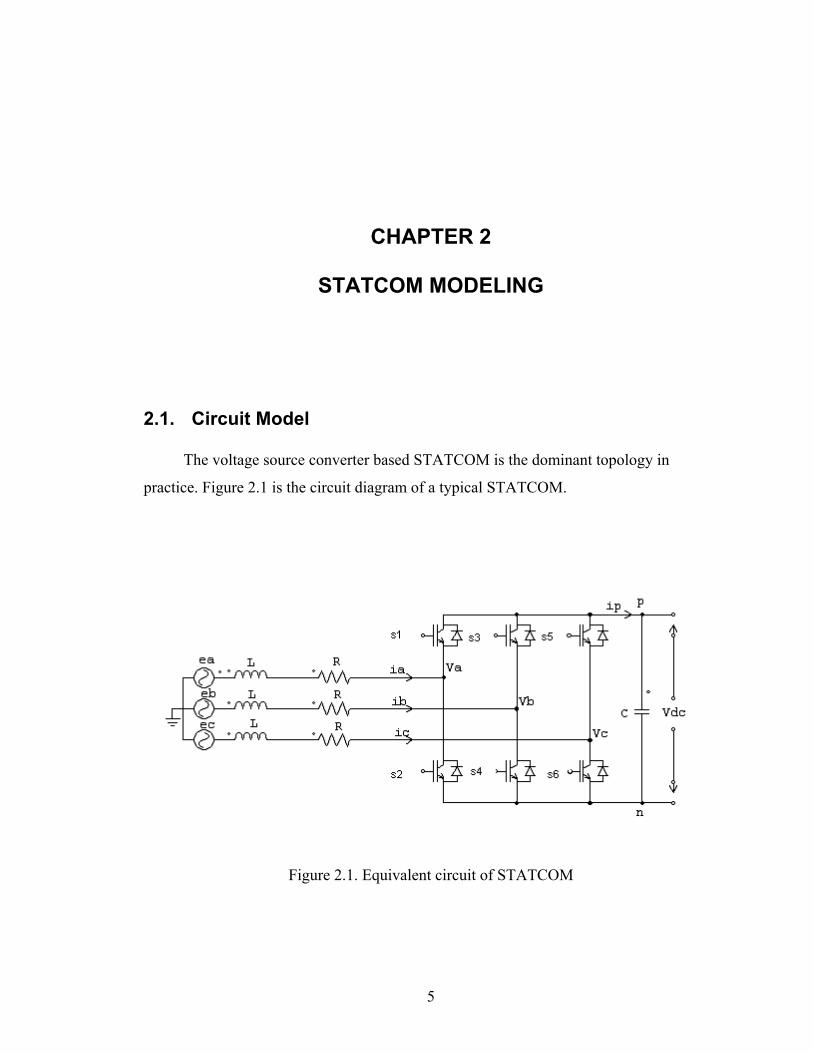
The voltage source converter based STATCOM is the dominant topology in
practice. Figure 2.1 is the circuit diagram of a typical STATCOM.
Figure 2.1. Equivalent circuit of STATCOM
5

Where
i line current; cba ii ,,
V converter phase voltage; cba VV ,,
AC source phase voltage; cba eee ,,
Vdc =Vpn DC side voltage;
i DC side current; p
L inductance of the line reactor;
R resistance of the line reactor;
C DC side capacitor,
2.2. Mathematic Model
Based on the equivalent circuit of STATCOM shown in Figure 2.1 we can derive
the mathematic model of STATCOM as fallow.
From power electronics principles we get
i (2.1)
−−−
=
ca
bc
ab
T
apcp
cpbp
bpap
p
iii
DDDDDD
Where
are switching functions and kpD cbak ,,=
31
=abi ( ), ba ii − )(31
cbbc ii −=i , )(31
acca ii −=i
6
and
. (2.2) VpnDDDDDD
VVVVVV
apcp
cppb
bpap
ac
cb
ba
−−−
=
−−−
From circuit principles we get
aaa
a VedtdiLRi −=+ (2.3)
bbb
b VedtdiLRi −=+ (2.4)
ccc
c VedtdiLRi −=+ (2.5)
and
)(31
dtdi
dtdi
Ldt
diL baab −= (2.6)
this equation can be expanded as below
RiVeVedt
diL abbbaa
ab −−−−= )]()[(31
RiVVee abbaba −−−−= )]()[(31 (2.7)
similarly we can get
RiVVeedt
diL bccbcbbc −−−−= )]()[(
31 (2.8)
RiVVeedt
diL caacacca −−−−= )]()[(
31 (2.9)
putting equations (2.7), (2.8) and (2.9) together we have
7
−
−−−
−
−−−
=
ca
bc
ab
ac
cb
ba
ac
cb
ba
ca
bc
ab
iii
LR
VVVVVV
Leeeeee
Liii
dtd
31
31 . (2.10)
By applying equation (2.2) to equation (2.10)
−
−−−
−
−−−
=
ca
bc
ab
apcp
cppb
bpap
ac
cb
ba
ca
bc
ab
iii
LRVpn
DDDDDD
Leeeeee
Liii
dtd
31
31 (2.11)
and
−−−
==
ca
bc
ab
T
apcp
cpbp
bpap
p
iii
DDDDDD
idt
dVpnC . (2.12)
It is common practical in power system application to transform 3 phase AC
dynamics into orthogonal components in a rotating reference frame. Here components are
referred to as the real and reactive components, those that lead to useful work and those
that do not respectively. From the power system theory we get the real and reactive
currents relative to a rotating reference frame with angular frequency ω as
(2.13)
=
c
b
a
q
d
iii
Pii
0
and
8
+−−−−
+−
=
21
21
21
)32sin()
32sin()sin(
)32cos()
32cos()cos(
32 πωπωω
πωπωω
ttt
ttt
P (2.14)
where
active current component, di
i reactive current component, q
then we have
=
−
=
−−−
=
−
0)(
31
31 1
q
d
a
c
b
c
b
a
ac
cb
ba
ca
bc
ab
ii
Tiii
iii
iiiiii
iii
(2.15)
where
++−
−
−−−
=−
1)31cos()
31sin(
1)cos()sin(
1)31cos()
31sin(
311
πωπω
ωω
πωπω
tt
tt
tt
T (2.16)
if we set T as the first two 2×3 subspace of matrix T , we can get
(2.17)
=
ca
bc
ab
q
d
iii
Tii
similarly we can get
9
(2.18)
=
ca
bc
ab
q
d
eee
Tee
(2.19)
=
ca
bc
ab
q
d
DDD
TDD
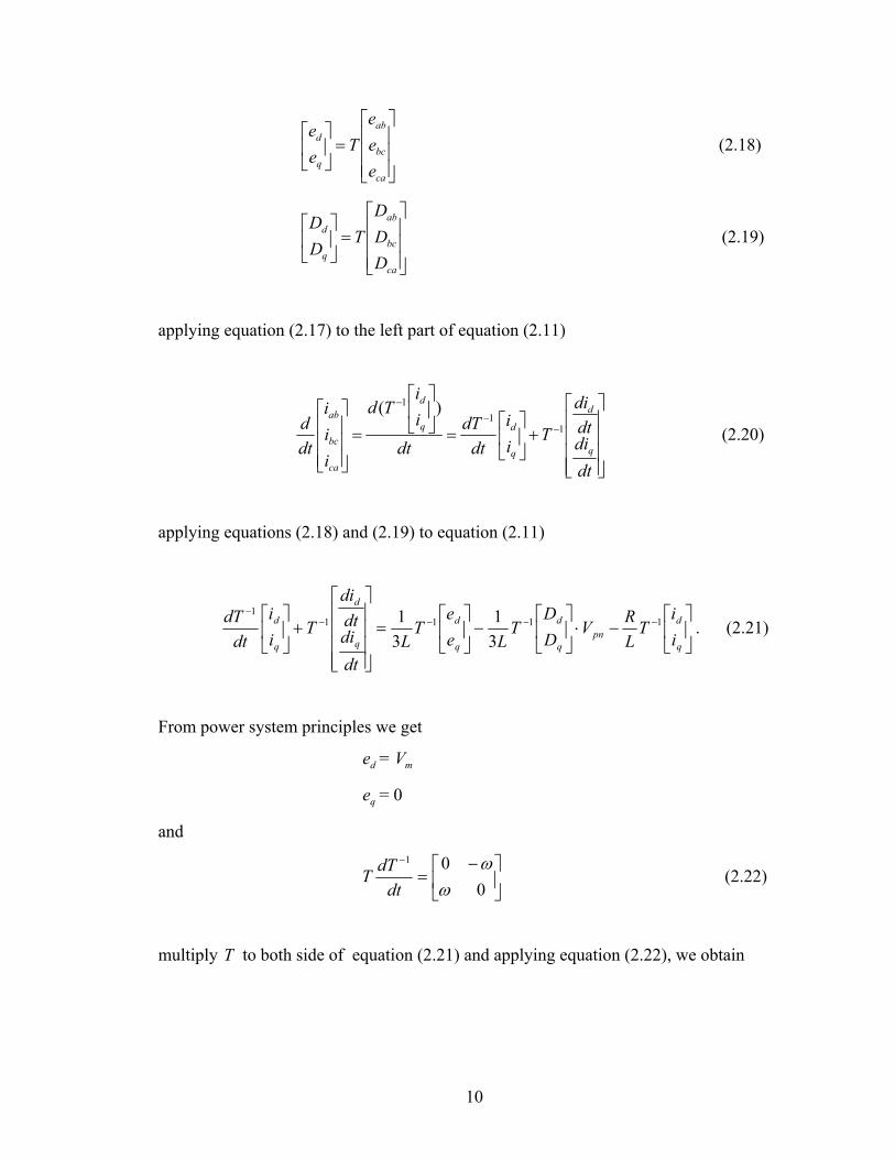
applying equation (2.17) to the left part of equation (2.11)
+
=
=
−
−
−
dtdidtdi
Tii
dtdT
dtii
Td
iii
dtd
q
d
q
dq
d
ca
bc
ab1
11 )(
(2.20)
applying equations (2.18) and (2.19) to equation (2.11)
−⋅
−
=
+
−−−−−
q
dpn
q
d
q
d
q
d
q
d
ii
TLRV
DD
TLe
eT
Ldtdidtdi
Tii
dtdT 1111
1
31
31 . (2.21)
From power system principles we get
= V de m
= 0 qe
and
−=
−
001
ωω
dtdTT (2.22)
multiply T to both side of equation (2.21) and applying equation (2.22), we obtain
10
mq
d
q
d
VL
Vdcii
LDq
LR
LDd
LR
dtdidtdi
+
−−−
−−=
00
31
3
3ω
ω. (2.22)
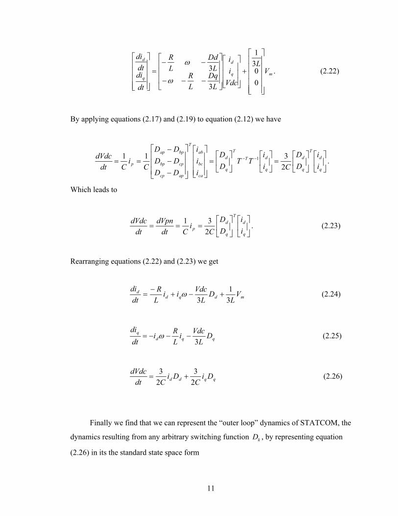
By applying equations (2.17) and (2.19) to equation (2.12) we have
=
=
−−−
== −−
q
dT
q
d
q
dT
T
q
d
ca
bc
ab
T
apcp
cpbp
bpap
p ii
DD
Cii
TTDD
iii
DDDDDD
Ci
CdtdVdc
2311 1 .
Which leads to
===
q
dT
q
dp i
iDD
Ci
CdtdVpn
dtdVdc
231 . (2.23)
Rearranging equations (2.22) and (2.23) we get
=dtdid
mdqd VL
DL
VdciiLR
31
3+−+
− ω (2.24)
qqdq D
LVdci
LRi
dtdi
3−−−= ω (2.25)
qqdd DiC
DiCdt
dVdc23
23
+= (2.26)
Finally we find that we can represent the “outer loop” dynamics of STATCOM, the
dynamics resulting from any arbitrary switching function , by representing equation
(2.26) in its the standard state space form
kD
11
m
dc
q
d
qd
q
d
q
d
VL
Vii
DC
DC
LD
LR
LD
LR
Vdcii
dtd
+
−−−
−−
=
00
31
023
23
3
3
ω
ω
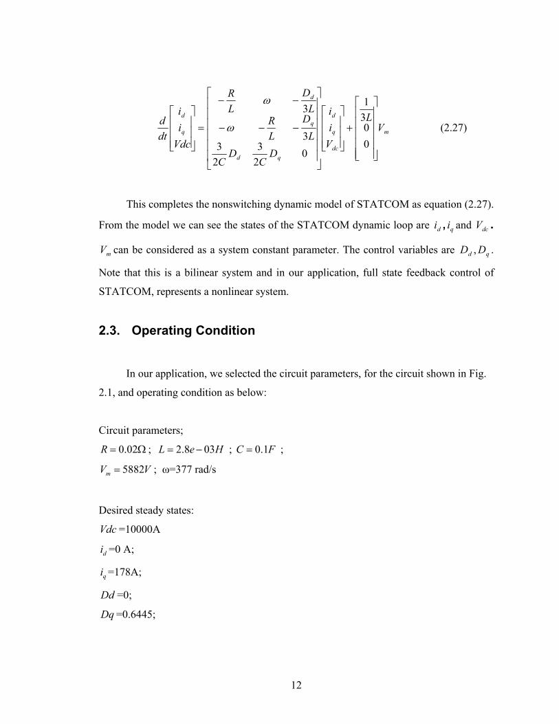
(2.27)
This completes the nonswitching dynamic model of STATCOM as equation (2.27).
From the model we can see the states of the STATCOM dynamic loop are i , i and V .
can be considered as a system constant parameter. The control variables are
Note that this is a bilinear system and in our application, full state feedback control of
STATCOM, represents a nonlinear system.
d q dc
qD, .mV dD
2.3. Operating Condition In our application, we selected the circuit parameters, for the circuit shown in Fig.
2.1, and operating condition as below:
Circuit parameters;
Ω= 02.0R ; ; HeL 038.2 −= FC 1.0= ;
VVm 5882= ; ω=377 rad/s
Desired steady states:
Vdc =10000A
di =0 A;
qi =178A;
Dd =0;
Dq =0.6445;
12

CHAPTER 3
ANALYSIS OF THE STATCOM MODEL
From the STATCOM mathematic model (2.27), we can see that it is a nonlinear
system. The problem then is how we can deal with the nonlinear characteristics in the
controlled STATCOM. There are different methods, which can be used to control a
nonlinear system. Since we know the operating points of the STATCOM we can use the
linearization method to cope with this nonlinear problem.
3.1 Linearization of STATCOM Model Here we linearize using the method of Jacobian. By using Jacobian matrix method,
we can linearize equation ( 2.27) to linear equations around a given operating point.
If is the function to be linaerized and ( )xf ( ) 13×ℜ∈xf then this Jacobian can be
∂∂
∂∂
∂∂
∂∂
∂∂
∂∂
∂∂
∂∂
∂∂
=∂∂
33
32
31
23
22
21
13
12
11
xf
xf
xf
xf
xf
xf
xf
xf
xf
xf (3.1)
For a nonlinear system, we may express the dynamics in the general vector
function form as . However pole assignment and LQR methods require us to
use a linear time invariant (LTI) presentation of the system as found in equation (3.2).
( uxfX ,=•
)
13
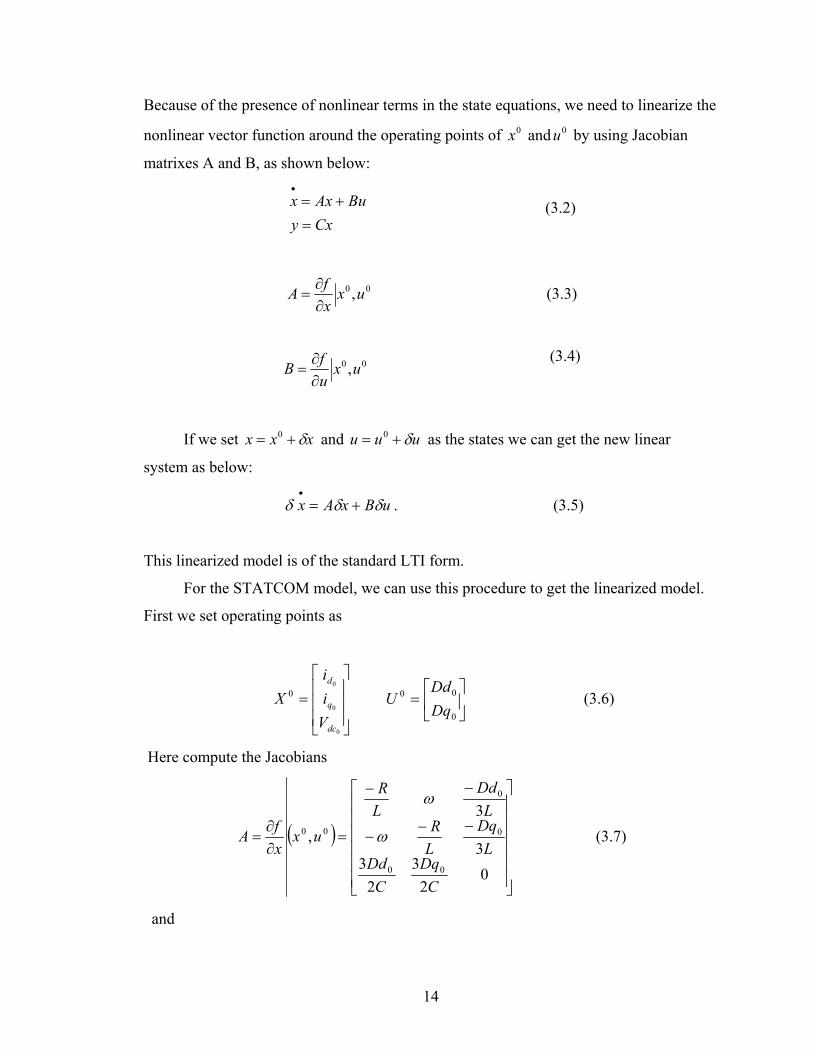
Because of the presence of nonlinear terms in the state equations, we need to linearize the
nonlinear vector function around the operating points of andu by using Jacobian
matrixes A and B, as shown below:
0x 0
(3.2) Cxy
BuAxx=
+=•
00 ,uxxfA
∂∂
= (3.3)
00 ,uxufB
∂∂
= (3.4)
If we set and as the states we can get the new linear
system as below:
xxx δ+= 0 uuu δ+= 0
. (3.5) uBxAx δδδ +=•
This linearized model is of the standard LTI form.
For the STATCOM model, we can use this procedure to get the linearized model.
First we set operating points as
U (3.6)
=
0
0
00
dc
q
d
Vii
X
=
0
00
DqDd
Here compute the Jacobians
( )
−−−
−−
=∂∂
=
02
32
33
3,
00
0
0
00
CDq
CDd
LDq
LR
LDd
LR
uxxfA ω
ω
(3.7)
and
14
( )
−
−
=∂∂
=
Ci
Ci
LV
LV
uxufB
qd
dc
dc
23
23
30
03
,
00
00 0
0
(3.8)
C is the identity matrix and will be ignored in the remaining discussion.
If we set 0~ xXX −= and 0~ uU −=U , we then get the small signal model of the
STATCOM as below:
UBXAX ~~~ +=•
(3.9)
Since Vm is constant therefore it would not exist in small signal model given by (3.9).
3.2 Open loop characteristics of STATCOM Model Having the linearized system state space model as equation (3.9), we can use the
linear system method to analyze the characteristics of STATCOM model. There are
several open loop system properties we need to know before we design the controller.
Although system observability and controllability are the properties of the system
presentation, these are two important criterions that must be established before any
attempt in controller design is done. These two characteristics of a system depend on the
state space presentations of the system. For a given system, different state space
presentations have different effects on the controller design algorithm.
Another important property of a system is its open loop dynamic response
characteristic that gives us not only the background information about the system
performance but also the guideline for controller design.
1. Obsevability and Controllability
The state space model of STATCOM has three state variables - i , , V . All of
them can be measured from the power system, which means the system is observable.
q di dc
15
However we only have two independent control inputs to the three system states,
we need to see if the system is controllable. In our case, the state matrix and the
input matrix , We need to see if the system controllability matrix Co is full rank.
33×ℜ∈A23×ℜ∈B
Where, Co= [A: AB : AAB]
From chapter 2.3 we know that given the follow component parameters
Ω= 02.0R ; ; mHL 8.2=
FC 1.0= ;V ; Vm 5882= srad /377=ω
The operating point is
dcV =10000A, i =0, i =178A; d q
0Dd =0, =0.6445; 0Dq
Thus we get
=
0 9.6675 0 9.6675 7.1429- 377.0000-
0 377.0000 7.1429- A
×+=
0.0027 0 1.1905- 0 0 1.1905-
0061.0e B
Thus Controllability matrix Co is
×+=
1.0420 0.0424- 0.0000-0.0424- 9.9165 0.00010.0000- 0.0001 9.9252
0101.0e Co
det ( ) =1.0254e+032 Co
16
The Co matrix has full rank, thus the linearized model is controllable. One topic of
the future work may be to examine this controllability for arbitrary operating point to
obtain a general knowledge of operating point controllability.
2. Eigenvalues and Dynamic Performance
The open loop linearized system’s eigenvalues are:
+=Λ
0.04- 3.7798i - 7.12-
3.7798i 7.12-×1.0 e-02
Since all the eigenvalues of the system are on the left hand of the plane, the system
is stable.
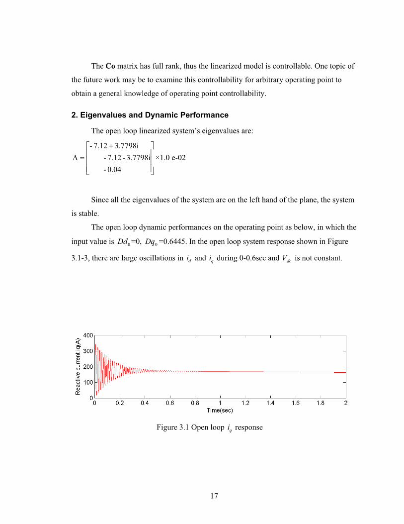
The open loop dynamic performances on the operating point as below, in which the
input value is =0, =0.6445. In the open loop system response shown in Figure
3.1-3, there are large oscillations in and during 0-0.6sec and V is not constant.
0Dd 0Dq
di qi dc
Figure 3.1 Open loop response qi
17
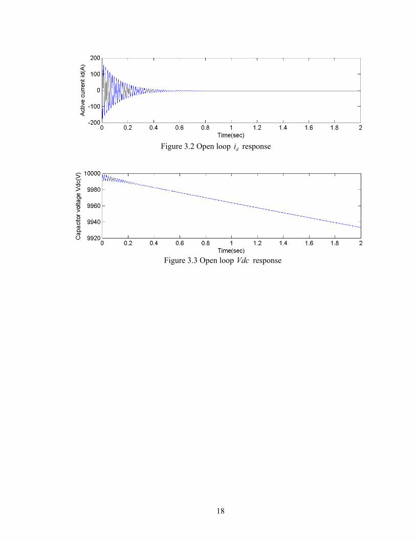
Figure 3.2 Open loop response di
Figure 3.3 Open loop Vdc response
18

CHAPTER 4
MULTIVARIABLE CONTROLLER DESIGN
Since the STATCOM is used for instantaneous reactive power compensation for
power systems, the response should be within one period of the power system [5]. The
frequency of the power system is 60 Hz, which means that one period is about 0.017sec.
Thus the transient response time should be less than 0.017sec. In the mean time the
voltage of the capacitor V should be kept constant [3]. The control effort of and
should be within [-1, +1], see [17].
qi
qi
dc Dd
Dq
In the practice of STATCOM application, the operating point shift from the desired
point. Thus another requirement for the controller is that the closed loop system should
be robust enough to tolerate the minor change of the operating point and the potential
change of the actual parameters of the STATCOM from those of the model.
There are several methods to implement this multivariable controller design. The
first choice for this multivariable design is an attempt to find an approximate model
through decoupling in which the controller design is decoupled into two or more single
input –output models. This is the common practical solution for many STATCOM [10],
[11], [12]. This method gives a simpler and more tractable subset of the system such that
we can design the controller as in Single Input Single Output (SISO) application by using
conventional PI control. However, decoupling this way leads to the STATCOM
performance become very sensitive about its operating point, [13]. Thus we choose use
other methods to design our controller that will be based on the coupled system model.
19

There are two main Multiple Input Multiple Output (MIMO) design methods: full state
feedback design and LQR design. We will discuss these two methods used in
STATCOM controller design.
4.1 Pole assignment controller design
A full state feedback controller based on the pole assignment method can improve
the system characteristics such that the closed loop system performance will satisfy the
requirement criteria.
4.1.1 Algorithm
For a given system:
(4.1) ;BuAxx +=•
Where,
is the state vector Nx ℜ∈
u is the input vector Pℜ∈
is the basis matrix NNA ×ℜ∈
is the input matrix PNB ×ℜ∈
If we set controller as:
u )()( tKxt −= . (4.2)
Then the closed loop state equation can be obtained as
. (4.3) )()()(.
txBKAtx −=
This state equation describes the system formed by combining the plant and the
controller. It is a homogeneous state equation, which has no input. The solution of this
state is given by:
(4.4) ).0()( )()( xetx txBKA−=
The state feedback controller )()( tKxtu −= drives the state to zero for arbitrary
initial conditions, provided that the closed loop poles ---the eigenvalues of --all )( BKA −
20

have negative real parts. By setting pole locations, we can make the closed loop system
not only stable but also satisfy a given set of transient specifications.
A state feedback gain K that yields the closed loop poles is
obtained by solving the equation:
,2,1 xpnpp ⋅⋅⋅⋅⋅⋅⋅⋅
det( )()2)(1() xpnspspsBKAsI −⋅⋅⋅⋅⋅⋅⋅⋅−−=+− . (4.5)
4.1.2 Eigenvalues Selection
The selection of closed loop system eigenvalues needs an understanding of the
system characteristics and the limitation of the actuator. Different pole locations
determine different system performance. This is the critical part of the controller design.
By comparing the system performance in simulation, we can select the suitable pole
locations as discussed in the following part.
4.1.3 Controller Design
We need a simulation loop to verify our controller performance before we validate
it in the circuit loop, and we also need the simulation loop to help us design the
controller. There are two tasks about the simulation: system loop and control loop. First,
we need to build the open loop system simulation loop, which can represent the
STATCOM dynamic performance. By using the STATCOM mathematic model, we get
the system open loop model in Simulink as that is a representation of equation (2.27).
With a loop, we can build the closed full state feedback loop as shown in Figure 4.1.
21
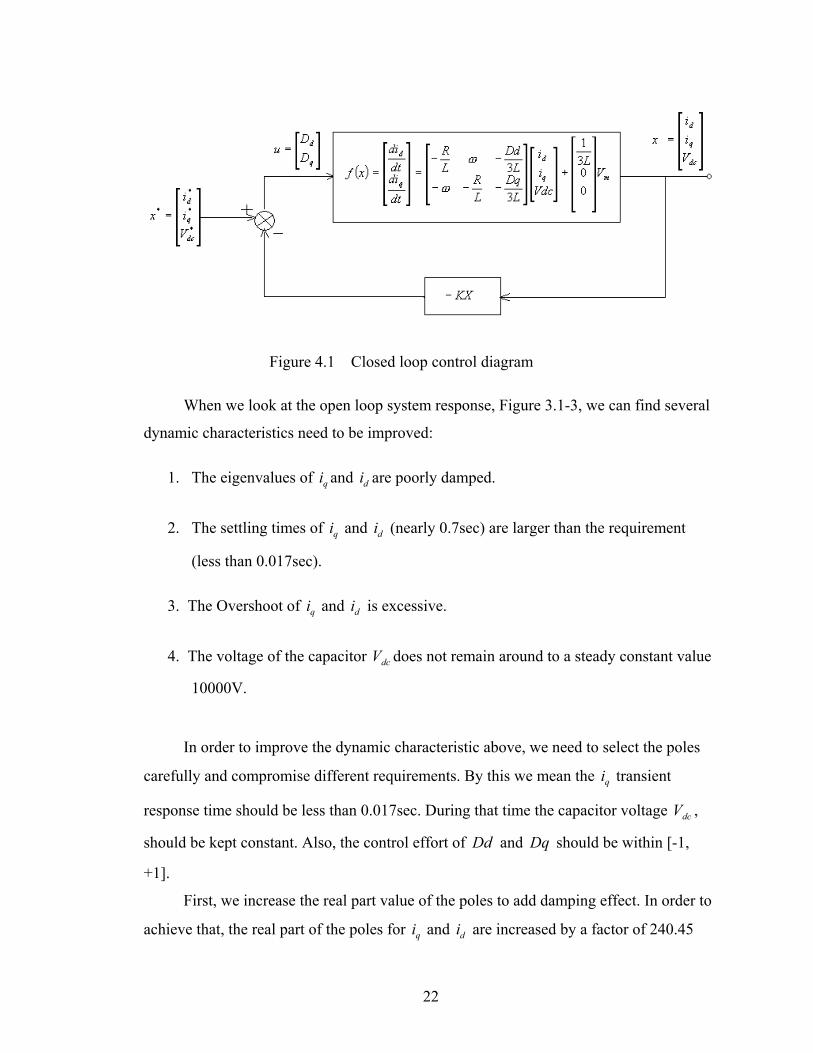
Figure 4.1 Closed loop control diagram
When we look at the open loop system response, Figure 3.1-3, we can find several
dynamic characteristics need to be improved:
1. The eigenvalues of i and are poorly damped. q di
2. The settling times of and i (nearly 0.7sec) are larger than the requirement
(less than 0.017sec).
qi d
3. The Overshoot of and i is excessive. qi d
4. The voltage of the capacitor V does not remain around to a steady constant value
10000V.
dc
In order to improve the dynamic characteristic above, we need to select the poles
carefully and compromise different requirements. By this we mean the i transient
response time should be less than 0.017sec. During that time the capacitor voltage V ,
should be kept constant. Also, the control effort of and should be within [-1,
+1].
q
dc
Dd Dq
First, we increase the real part value of the poles to add damping effect. In order to
achieve that, the real part of the poles for and i are increased by a factor of 240.45 qi d
22
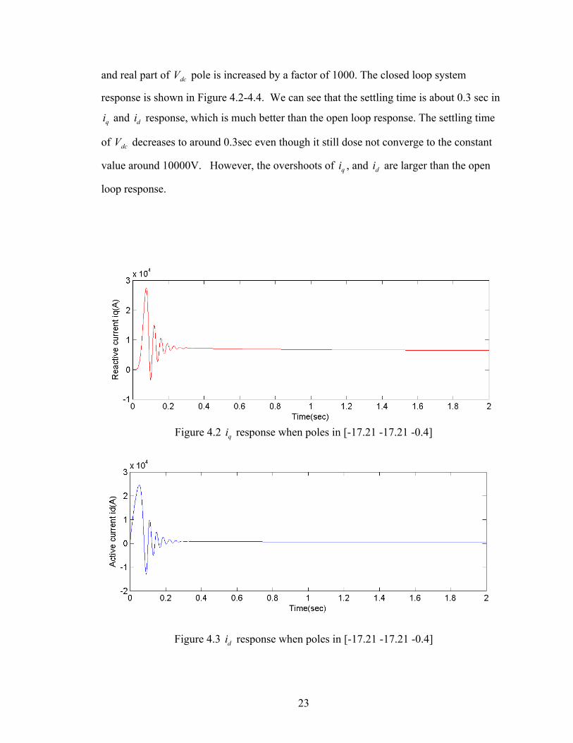
and real part of V pole is increased by a factor of 1000. The closed loop system
response is shown in Figure 4.2-4.4. We can see that the settling time is about 0.3 sec in
and i response, which is much better than the open loop response. The settling time
of V decreases to around 0.3sec even though it still dose not converge to the constant
value around 10000V. However, the overshoots of , and are larger than the open
loop response.
dc
qi d
dc
qi di
Figure 4.2 response when poles in [-17.21 -17.21 -0.4] qi
Figure 4.3 i response when poles in [-17.21 -17.21 -0.4] d
23
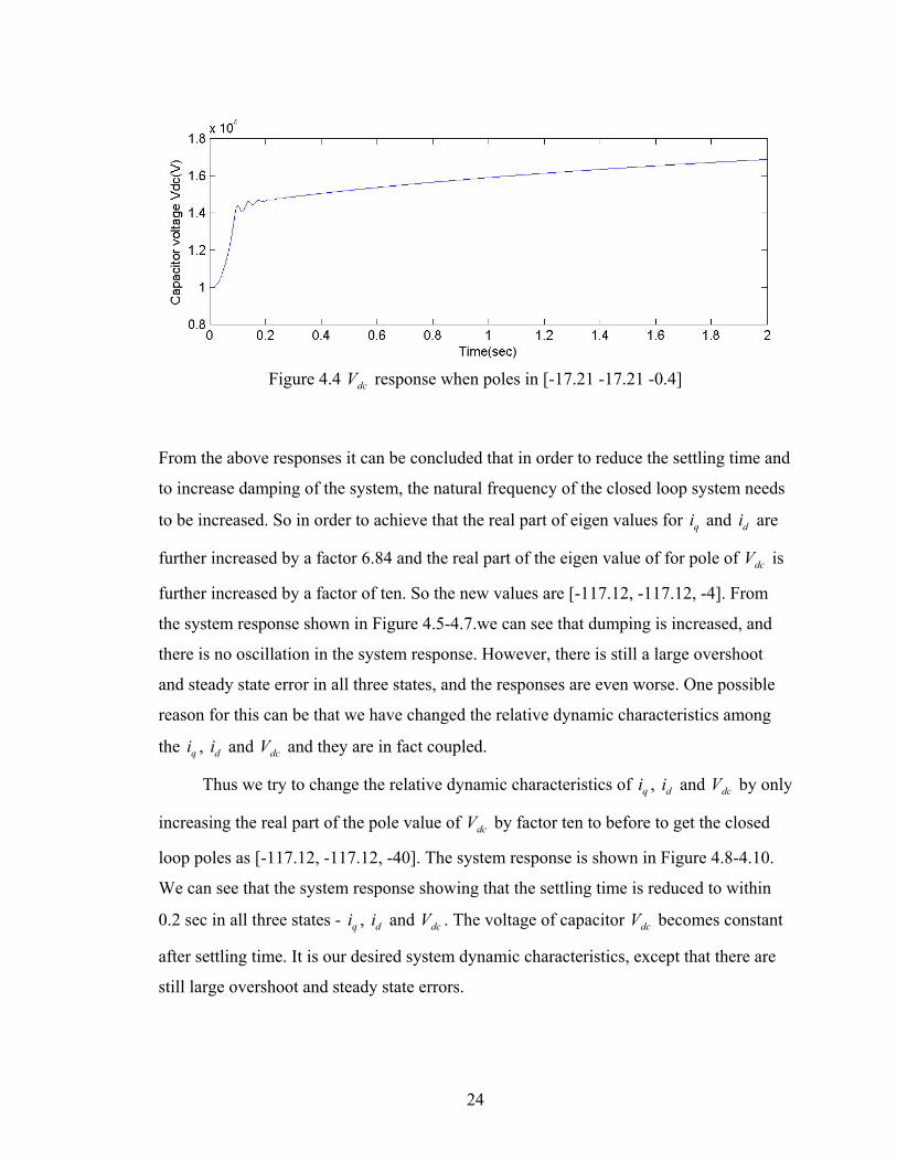
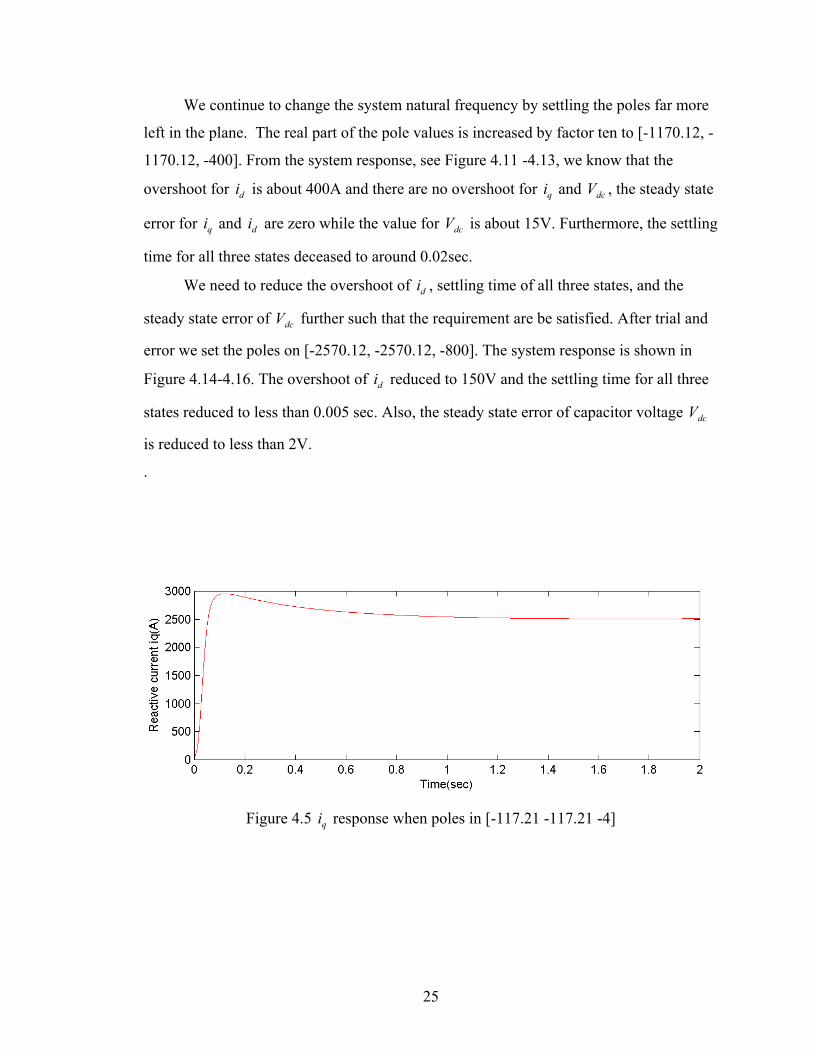
Figure 4.4 V response when poles in [-17.21 -17.21 -0.4] dc
From the above responses it can be concluded that in order to reduce the settling time and
to increase damping of the system, the natural frequency of the closed loop system needs
to be increased. So in order to achieve that the real part of eigen values for i and are
further increased by a factor 6.84 and the real part of the eigen value of for pole of V is
further increased by a factor of ten. So the new values are [-117.12, -117.12, -4]. From
the system response shown in Figure 4.5-4.7.we can see that dumping is increased, and
there is no oscillation in the system response. However, there is still a large overshoot
and steady state error in all three states, and the responses are even worse. One possible
reason for this can be that we have changed the relative dynamic characteristics among
the , and V and they are in fact coupled.
q di
dc
qi di dc
Thus we try to change the relative dynamic characteristics of i , i and V by only
increasing the real part of the pole value of V by factor ten to before to get the closed
loop poles as [-117.12, -117.12, -40]. The system response is shown in Figure 4.8-4.10.
We can see that the system response showing that the settling time is reduced to within
0.2 sec in all three states - i , i and V . The voltage of capacitor V becomes constant
after settling time. It is our desired system dynamic characteristics, except that there are
still large overshoot and steady state errors.
q
dc
d dc
dc
q d dc
24
We continue to change the system natural frequency by settling the poles far more
left in the plane. The real part of the pole values is increased by factor ten to [-1170.12, -
1170.12, -400]. From the system response, see Figure 4.11 -4.13, we know that the
overshoot for i is about 400A and there are no overshoot for and V , the steady state
error for i and are zero while the value for V is about 15V. Furthermore, the settling
time for all three states deceased to around 0.02sec.
d
i
qi dc
q d dc
We need to reduce the overshoot of , settling time of all three states, and the
steady state error of V further such that the requirement are be satisfied. After trial and
error we set the poles on [-2570.12, -2570.12, -800]. The system response is shown in
Figure 4.14-4.16. The overshoot of i reduced to 150V and the settling time for all three
states reduced to less than 0.005 sec. Also, the steady state error of capacitor voltage V
is reduced to less than 2V.
di
dc
d
dc
.
Figure 4.5 i response when poles in [-117.21 -117.21 -4] q
25
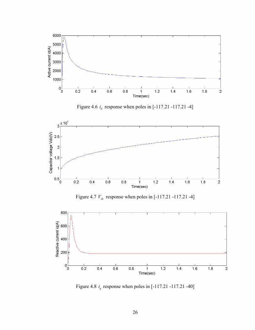
Figure 4.6 response when poles in [-117.21 -117.21 -4] di
Figure 4.7 V response when poles in [-117.21 -117.21 -4] dc
Figure 4.8 i response when poles in [-117.21 -117.21 -40] q
26
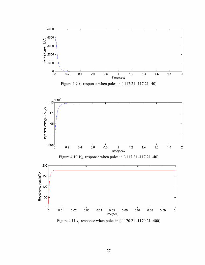
Figure 4.9 response when poles in [-117.21 -117.21 -40] di
Figure 4.10 V response when poles in [-117.21 -117.21 -40] dc
Figure 4.11 i response when poles in [-1170.21 -1170.21 -400] q
27
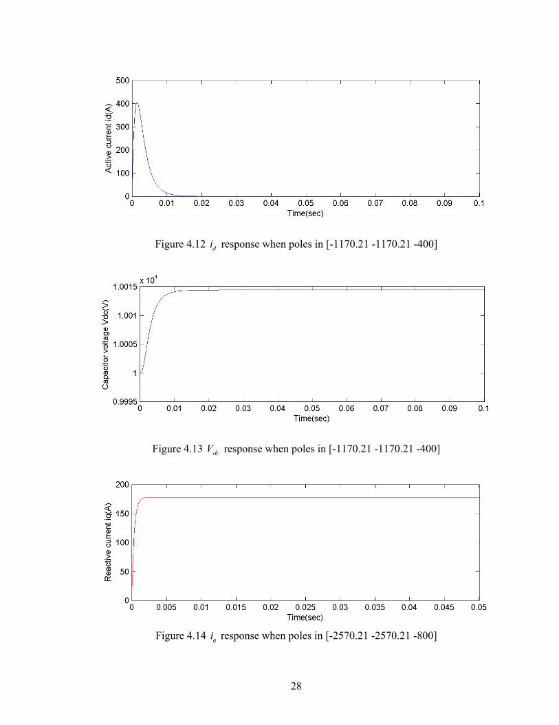
Figure 4.12 response when poles in [-1170.21 -1170.21 -400] di
Figure 4.13 V response when poles in [-1170.21 -1170.21 -400] dc
Figure 4.14 i response when poles in [-2570.21 -2570.21 -800] q
28
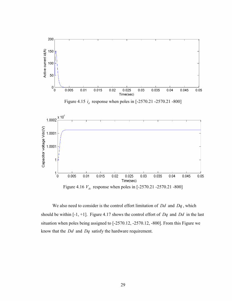
Figure 4.15 response when poles in [-2570.21 -2570.21 -800] di
Figure 4.16 V response when poles in [-2570.21 -2570.21 -800] dc
We also need to consider is the control effort limitation of and , which
should be within [-1, +1]. Figure 4.17 shows the control effort of and in the last
situation when poles being assigned to [-2570.12, -2570.12, -800]. From this Figure we
know that the and satisfy the hardware requirement.
Dd
Dq
Dq
Dd
Dd Dq
29

Figure 4.17 Control effort and when pole in[-2501.12, -2570.12, -800] Dd Dq
4.2 LQR Controller Design
Another MIMO design approach is the optimal control method linear quadratic
regulator (LQR). The idea is to transfer the designer’s iteration on pole locations as used
in full state feedback to iterations on the elements in a cost function, . This method
determines the feedback gain matrix that minimizes in order to achieve some
compromise between the use of control effort, the magnitude, and the speed of response
that will guarantee a stable system.
J
J
4.2.1 Algorithm
For a given system:
(4.6) ;BuAxx +=•
determine the matrix K of the LQR vector
u )()( tKxt −= (4.7)
so in order to minimize the performance index,
30
(4.8) ∫∞
+=0
)( dtRuuQxxJ TT
where Q and R are the positive-definite Hermitian or real symmetric matrix. Note
that the second term on the right side account for the expenditure of the energy on the
control efforts. The matrix Q and R determine the relative importance of the error and
the expenditure of this energy.
From the above equations we get
(4.9) ∫∫∞∞
+=+=00
)()( xdtRKKQxdtRKxKxQxxJ TTTTT
following the discussion given in solving the parameter-optimization problem,
we set
)()( PxxdtdxRKKQx TTT −=+ (4.10)
then we obtain
(4.11) ••
−−=+ xPxPxxxRKKQx TT
TT )( xBKAPPBKAx TT )]()[( −+−−=
comparing both sides of the above equation and note that this equation must hold true for
any x, we require that
( . (4.12) )()() RKKQBKAPPBKA TT +−=−+−
Since R has been assumed to be a positive-definite Hermitian or real symmetric
matrix, we can write
TTR T=
where T is a nonsingular matrix.
and
. (4.13) 0])([])([ 111 =+−−−++ −−− QPBPBRPBTTKPBTTKPAPA TTTTTTT
The minimization of with respect to J K requires the minimization of
. (4.14) xPBTTKPBTTKx TTTTTT ])([])([ 11 −− −−
Which this equation is nonnegative, the minimum occurs when it is zero, or when
TK . (4.15) PBT TT 1)( −=
Hence
. (4.16) PBRPBTTK TTT 111 )( −−− ==
31
Thus we get a control law as
u (4.17) )()()( 1 tPxBRtKxt T−−=−=
in which P must satisfy the reduced Riccati equation:
(4.18) 01 =+−+ − QPBPBRPAPA TT
4.2.2 Weight Matrix Selection
The LQR design selects the weight matrix Q and R such that the performances of
the closed loop system can satisfy the desired requirements mentioned earlier.
The selection of Q and R is weakly connected to the performance specifications,
and a certain amount of trial and error is required with an interactive computer simulation
before a satisfactory design results.
4.2.3 Controller Design
Since the matrix Q and R are symmetric so there are 6 distinct elements in Q and 3
distinct elements in R for a total of 9 distinct elements need to be selected. And also the
matrix Q and R should satisfy the positive definitions. One practical method is to set Q
and R to be diagonal matrix such that only five elements need to be decided. The value of
the elements in Q and R is related to its contribution to the cost function J.
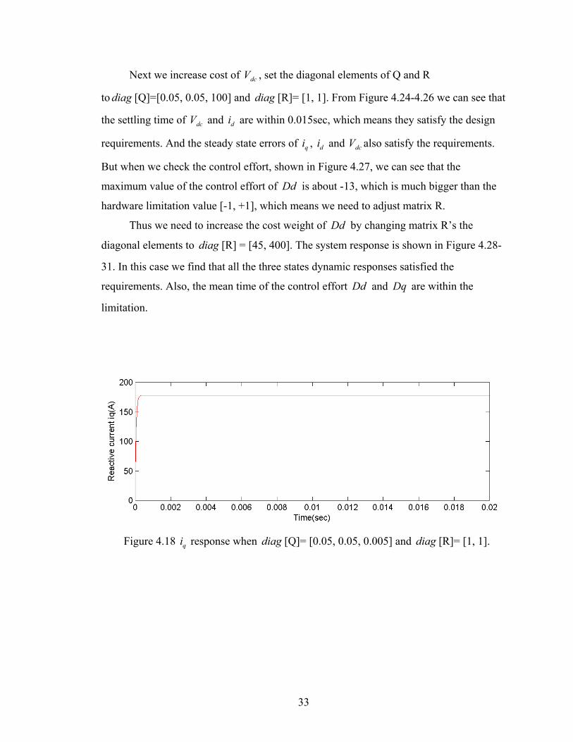
In our case, the response requirement of i and are the same, but the response
requirement of V is slow. Thus we first select the diagonal elements of Q and R as
[Q]= [0.05, 0.05, 0.005] and [R]= [1, 1]. The system response is shown in
Figure 4.18-4.20. We can find that the response of is perfect but the i and V do not
converge within 2 sec.
q di
dc
diag diag
qi d dc
We need pay more cost weight to V in order to satisfy the requirement. We set
diagonal elements of Q and R to [Q]= [0.05, 0.05, 0.01] and diag [R]= [1, 1]. The
system response is shown in Figure 4.21-4.23. The response of V and i converge to
the desired constant value this time, but the settling time is about 0.6sec, which is much
higher than the requirement (less than 0.017 sec).
dc
diag
dc d
32
Next we increase cost of V , set the diagonal elements of Q and R
to [Q]=[0.05, 0.05, 100] and diag [R]= [1, 1]. From Figure 4.24-4.26 we can see that
the settling time of V and are within 0.015sec, which means they satisfy the design
requirements. And the steady state errors of , and V also satisfy the requirements.
But when we check the control effort, shown in Figure 4.27, we can see that the
maximum value of the control effort of is about -13, which is much bigger than the
hardware limitation value [-1, +1], which means we need to adjust matrix R.
dc
diag
dc di
qi di dc
Dd
Thus we need to increase the cost weight of by changing matrix R’s the
diagonal elements to [R] = [45, 400]. The system response is shown in Figure 4.28-
31. In this case we find that all the three states dynamic responses satisfied the
requirements. Also, the mean time of the control effort and are within the
limitation.
Dd
diag
Dd Dq
Figure 4.18 i response when [Q]= [0.05, 0.05, 0.005] and [R]= [1, 1]. q diag diag
33
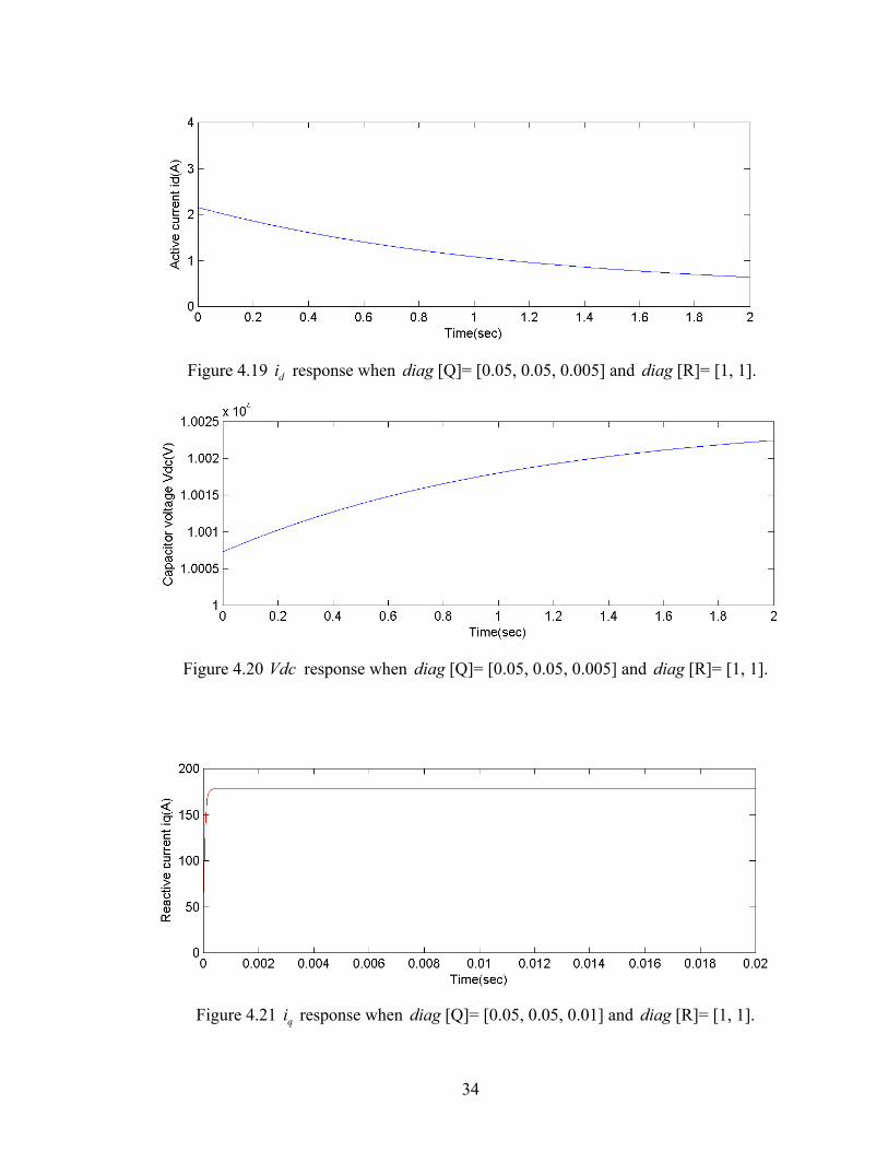
Figure 4.19 i response when [Q]= [0.05, 0.05, 0.005] and diag [R]= [1, 1]. d diag
Figure 4.20 Vdc response when [Q]= [0.05, 0.05, 0.005] and diag [R]= [1, 1]. diag
Figure 4.21 i response when [Q]= [0.05, 0.05, 0.01] and [R]= [1, 1]. q diag diag
34
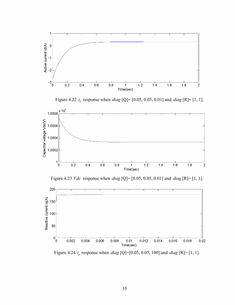
Figure 4.22 i response when [Q]= [0.05, 0.05, 0.01] and diag [R]= [1, 1]. d diag
Figure 4.23 Vdc response when [Q]= [0.05, 0.05, 0.01] and [R]= [1, 1]. diag diag
Figure 4.24 i response when [Q]=[0.05, 0.05, 100] and diag [R]= [1, 1]. q diag
35
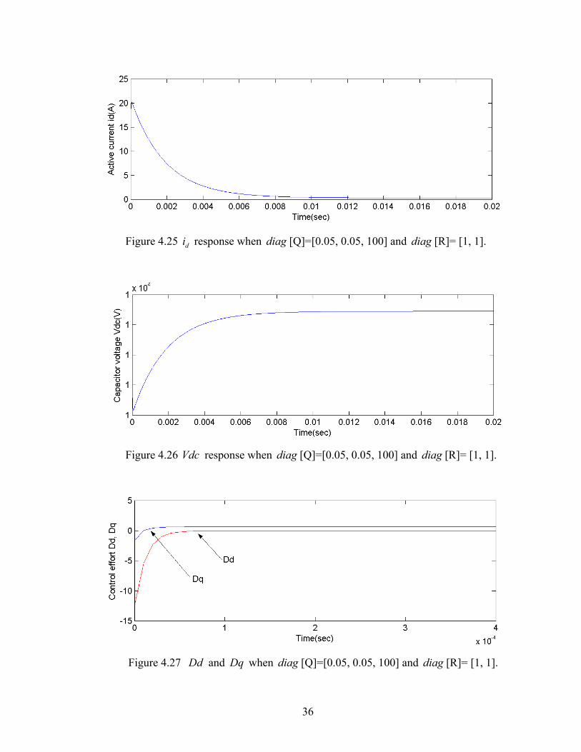
Figure 4.25 i response when [Q]=[0.05, 0.05, 100] and [R]= [1, 1]. d diag diag
Figure 4.26 Vdc response when [Q]=[0.05, 0.05, 100] and [R]= [1, 1]. diag diag
Figure 4.27 and when [Q]=[0.05, 0.05, 100] and [R]= [1, 1]. Dd Dq diag diag
36
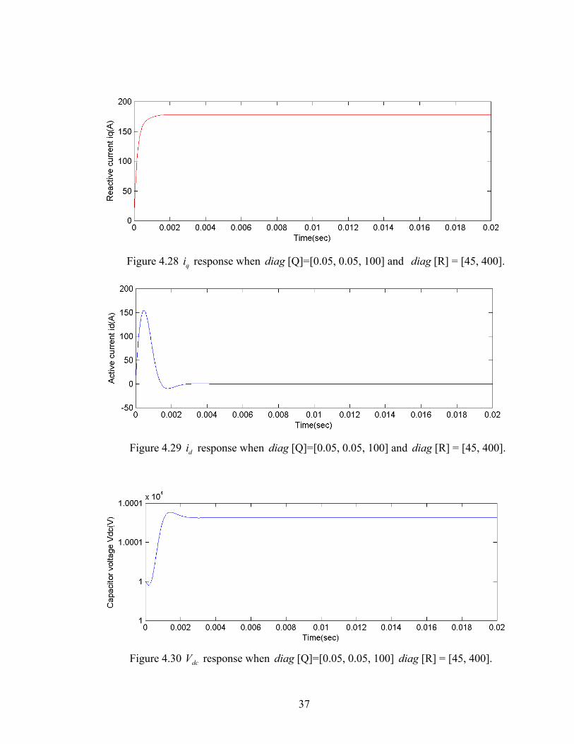
Figure 4.28 i response when [Q]=[0.05, 0.05, 100] and [R] = [45, 400]. q diag diag
Figure 4.29 i response when [Q]=[0.05, 0.05, 100] and [R] = [45, 400]. d diag diag
Figure 4.30 V response when [Q]=[0.05, 0.05, 100] [R] = [45, 400]. dc diag diag
37
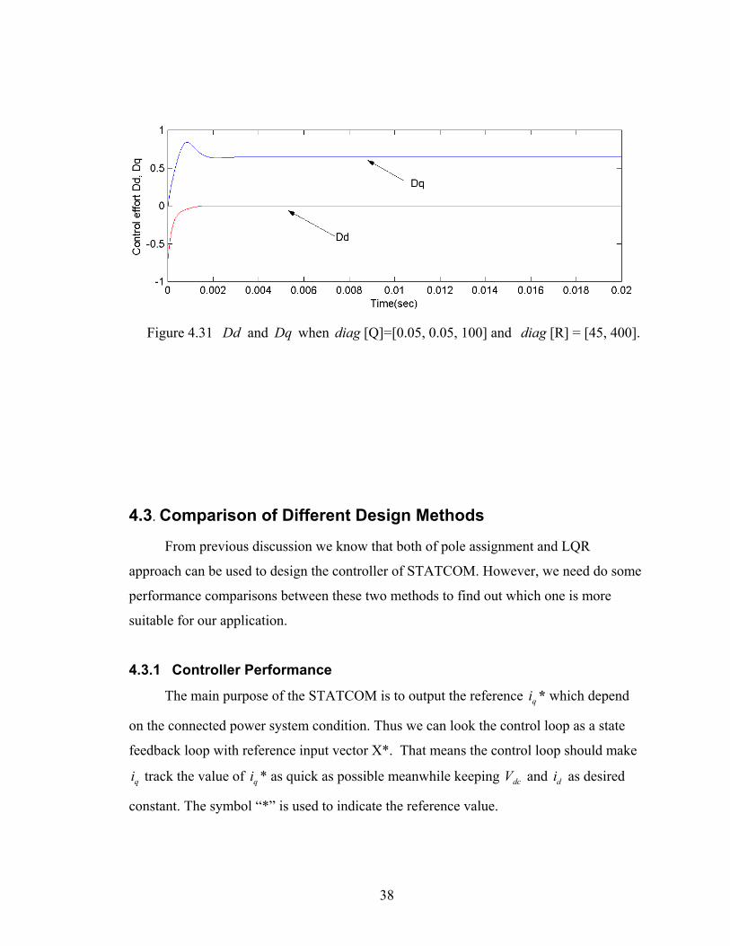
Figure 4.31 and when [Q]=[0.05, 0.05, 100] and [R] = [45, 400]. Dd Dq diag diag
4.3. Comparison of Different Design Methods
From previous discussion we know that both of pole assignment and LQR
approach can be used to design the controller of STATCOM. However, we need do some
performance comparisons between these two methods to find out which one is more
suitable for our application.
4.3.1 Controller Performance
The main purpose of the STATCOM is to output the reference i * which depend
on the connected power system condition. Thus we can look the control loop as a state
feedback loop with reference input vector X*. That means the control loop should make
track the value of * as quick as possible meanwhile keeping V and as desired
constant. The symbol “*” is used to indicate the reference value.
q
qi qi dc di
38

Although these two control methods show us almost the same good performance
on the operating point, it is necessary to investigate their robustness. So we need to see
the system performance when * change from its operating point (178A). qi
First we make the * as a step change from 178A to 267A (increase 50%). Figure
4.32 show the system response by using pole assignment method. Figure 4.33 show the
system response by using LQR method. In each loop we set * have step change from
178A to 267A at the time of 0.015sec. Both of them show their good robust
characteristics to the change of *.
qi
qi
qi
Then we make the i * as a step change from 267A (increase 50% from 178A) to
89A (decrease 50% from 178A). Figure 4.34 show the system response by using pole
assignment method. Figure 4.35 show the system response by using LQR method. In
each loop we set * have step change from 267A (+50%) to 89A (-50%) at the time of
0.015sec. Again, both of them show their good robust characteristics to the change of *.
q
qi
qi
4.3.2 Pole Assignment –LQR Design Procedure Comparison
1. Pole assignment method
Pole location must be chosen carefully and wisely, which needs deep insight of the
system characteristics. Also, for the multi-input multi-output system as in this case, the
gain matrix K is not uniquely determined by the resulting equations. Thus it is not easy
to use pole assignment method to design a MIMO system. We need higher feedback gain
to reduce the system response time and attenuate disturbances that might enter the
system. But higher gain leads to higher input that is limited by the hardware.
39
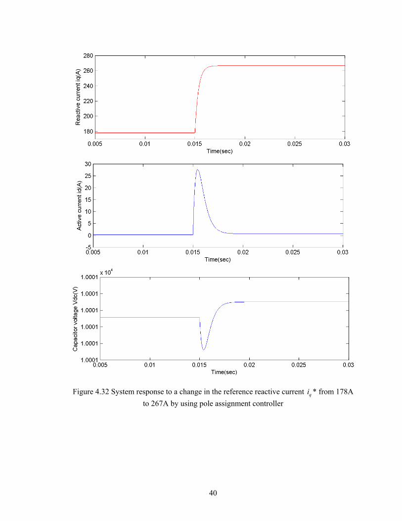
Figure 4.32 System response to a change in the reference reactive current i * from 178A to 267A by using pole assignment controller
q
40
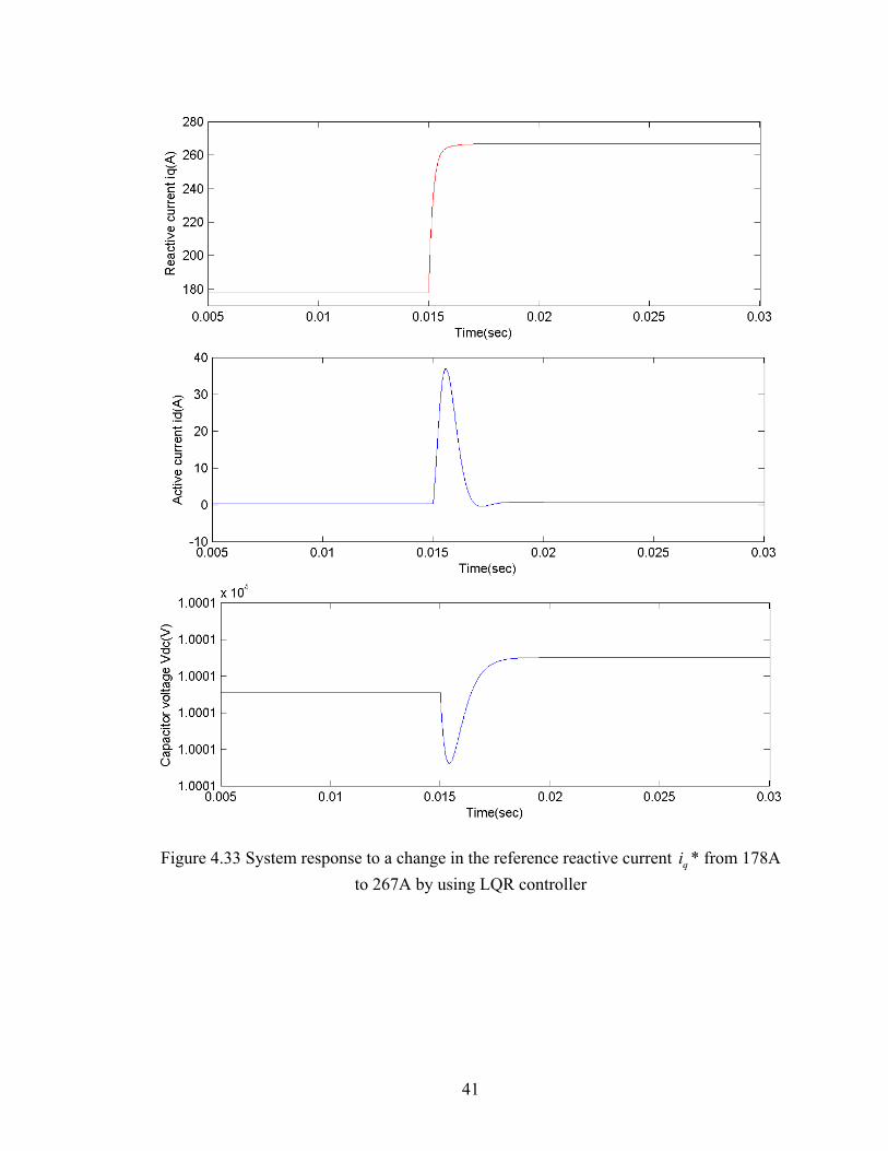
Figure 4.33 System response to a change in the reference reactive current i * from 178A to 267A by using LQR controller
q
41
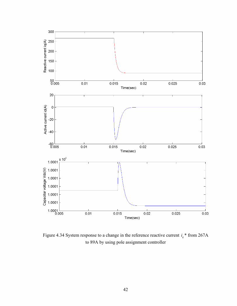
Figure 4.34 System response to a change in the reference reactive current i * from 267A to 89A by using pole assignment controller
q
42
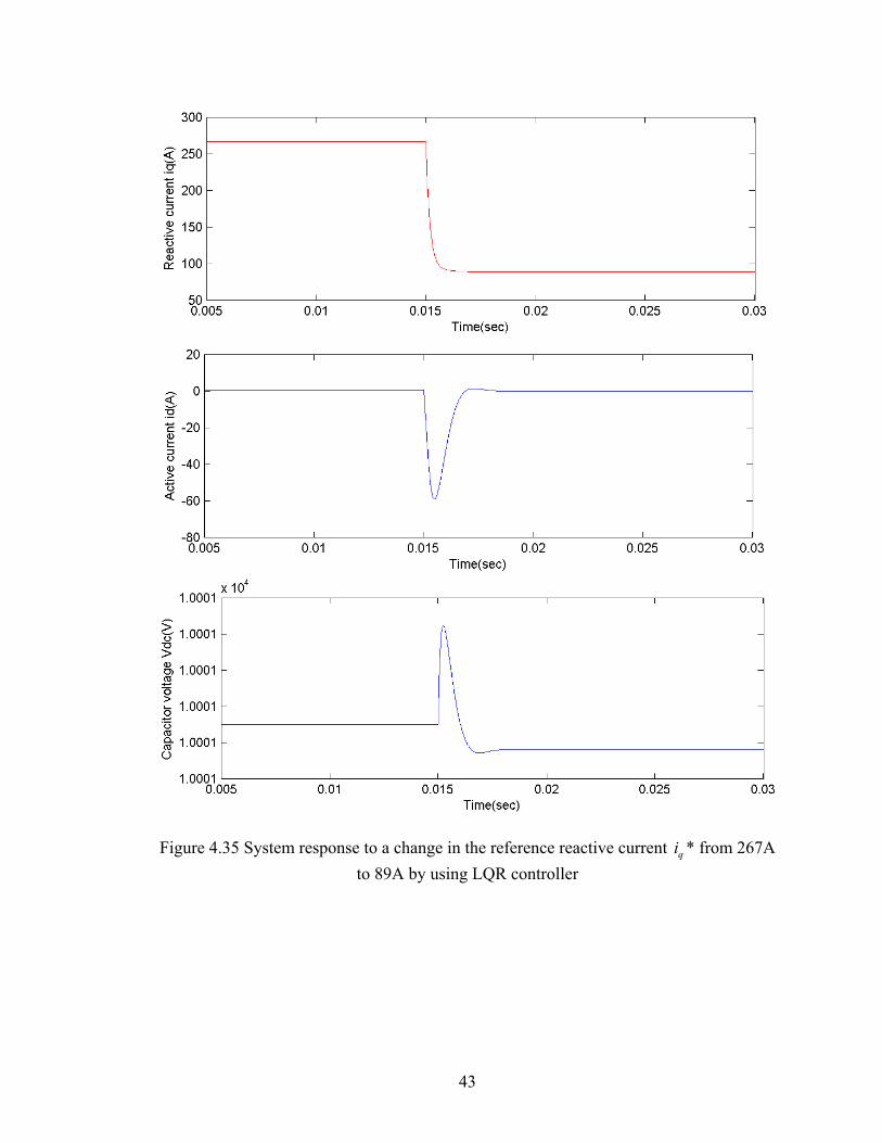
Figure 4.35 System response to a change in the reference reactive current i * from 267A to 89A by using LQR controller
q
43

4.3.3 Pole Assignment –LQR Design Procedure Comparison
2. Pole assignment method
Pole location must be chosen carefully and wisely, which needs deep insight of the
system characteristics. Also, for the multi-input multi-output system as in this case, the
gain matrix K is not uniquely determined by the resulting equations. Thus it is not easy
to use pole assignment method to design a MIMO system. We need higher feedback gain
to reduce the system response time and attenuate disturbances that might enter the
system. But higher gain leads to higher input that is limited by the hardware.
Thus we need to make a compromise between the input energy and output
performance and pay lots of attention while selecting the poles. It is still hard to find a
solution that can satisfy all the requirements.
3. LQR method
By using LQR, we can use all the freedom of MIMO system and achieve some
compromise between the use of control effort and system performance, and can also
guarantee a stable system.
We still need to specify the parameters (Q and R) of the cost function based on
the physical specifications. But it is relatively easy to achieve all the requirements. The
minimum value of leads to an unique solution of
J
J K , gain matrix.
The quadratic cost function provides us with performance trade-offs among various
performance criteria. The relationship between cost function weights and the
performance criteria hold for high order and multiple-input system like STATCOM.
Therefore it enables the systematic design for multivariable systems.
The selection of Q and R also need a certain amount of trial and error before a
satisfactory design results.
4. When sensor noise or system disturbance exist
Both of the two design procedures, pole assignment and LQR, make the
assumption that there is no sensor noise or system disturbance inputs to the closed loop
systems. This is a fairly restrictive problem statement, since real world control systems
are subject to noise and disturbance inputs, especially STATCOM. The circuit of
44

STATCOM is a switching circuit rather than a continuous circuit. There are significant
higher order harmonics that exist in the system. So, in the future work we need to
consider these disturbances in real implementations. There is no way to do this for pole
assignment design approach. But if we can classify the type of disturbances, we can
minimize their effect during the controller design procedure by using stochastic optimal
methods such as linear quadratic gaussian method LQG [22].
45
CHAPTER 5
CIRCUIT VALIDATION WITH BOTH CONTROL METHODS
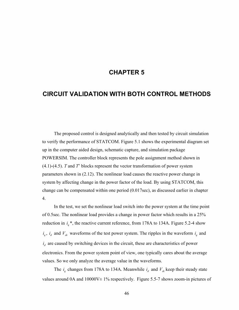
The proposed control is designed analytically and then tested by circuit simulation
to verify the performance of STATCOM. Figure 5.1 shows the experimental diagram set
up in the computer aided design, schematic capture, and simulation package
POWERSIM. The controller block represents the pole assignment method shown in
(4.1)-(4.5). T and T’ blocks represent the vector transformation of power system
parameters shown in (2.12). The nonlinear load causes the reactive power change in
system by affecting change in the power factor of the load. By using STATCOM, this
change can be compensated within one period (0.017sec), as discussed earlier in chapter
4.
In the test, we set the nonlinear load switch into the power system at the time point
of 0.5sec. The nonlinear load provides a change in power factor which results in a 25%
reduction in *, the reactive current reference, from 178A to 134A. Figure 5.2-4 show
, i and V waveforms of the test power system. The ripples in the waveform i and
are caused by switching devices in the circuit, these are characteristics of power
electronics. From the power system point of view, one typically cares about the average
values. So we only analyze the average value in the waveforms.
qi
dcqi
di
d q
The changes from 178A to 134A. Meanwhile i and V keep their steady state
values around 0A and 10000V± 1% respectively. Figure 5.5-7 shows zoom-in pictures of
qi d dc
46

these waveforms. From the waveforms we can see that the i can track the change within
0.006sec. The transient response of i and V are similarly fast.
q
d dc
The test results show that the STATCOM can compensate the reactive power
effectively and the control for STATCOM is good enough to ensure the fast reactive
power compensation.
Figure 5.8-13 show the results on the same situation by using LQR controller. We
found that the results are relatively identical to those by using pole assignment. Even
though the gains determined vary by as much as 12%.
Considerable effort in this controller design at this point came from Dr. Li,
Electrical and Computer Engineering Department of Florida State University. Dr. Li
contributed simulation and modeling support that directly impacted simulation results
shown in Fig.5.1 to Fig.5.13.
47
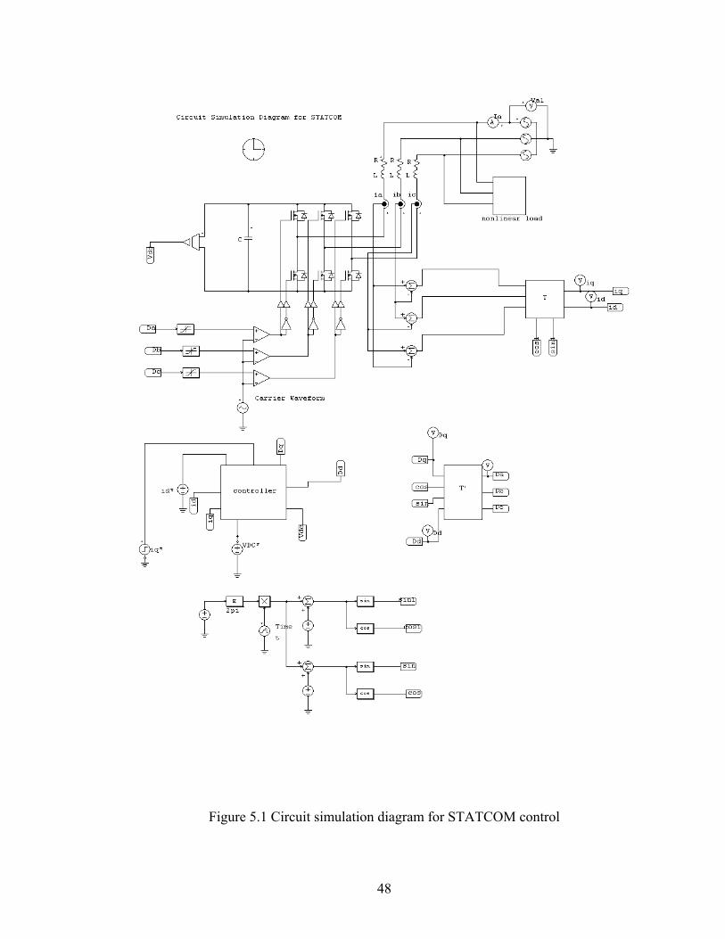
Figure 5.1 Circuit simulation diagram for STATCOM control
48
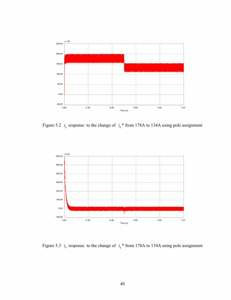
Figure 5.2 response to the change of * from 178A to 134A using pole assignment qi qi
Figure 5.3 i response to the change of i * from 178A to 134A using pole assignment d q
49
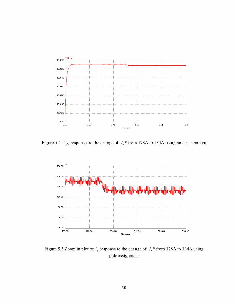
Figure 5.4 V response to the change of i * from 178A to 134A using pole assignment dc q
Figure 5.5 Zoom in plot of i response to the change of i * from 178A to 134A using
pole assignment q q
50
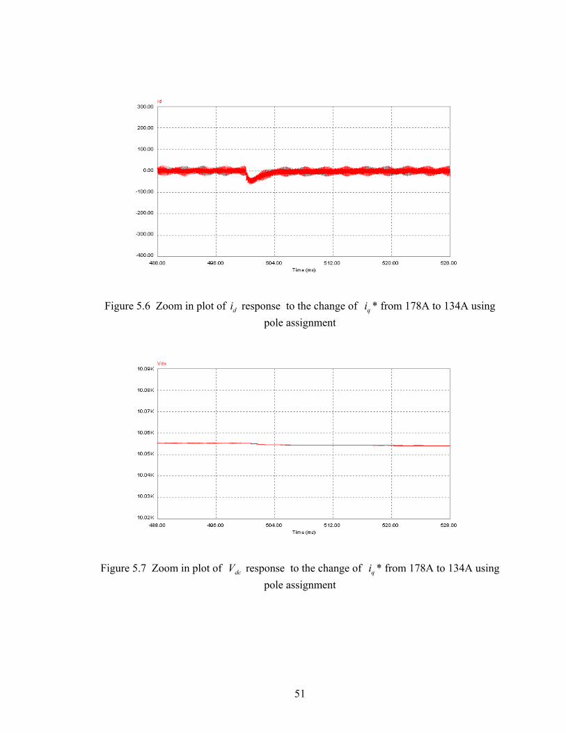
Figure 5.6 Zoom in plot of response to the change of * from 178A to 134A using
pole assignment di qi
Figure 5.7 Zoom in plot of V response to the change of i * from 178A to 134A using
pole assignment dc q
51
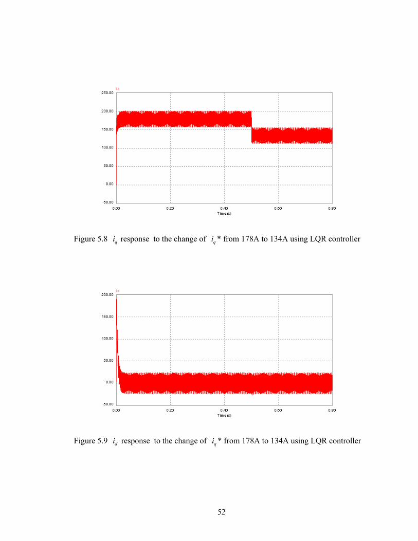
Figure 5.8 i response to the change of i * from 178A to 134A using LQR controller q q
Figure 5.9 i response to the change of i * from 178A to 134A using LQR controller d q
52
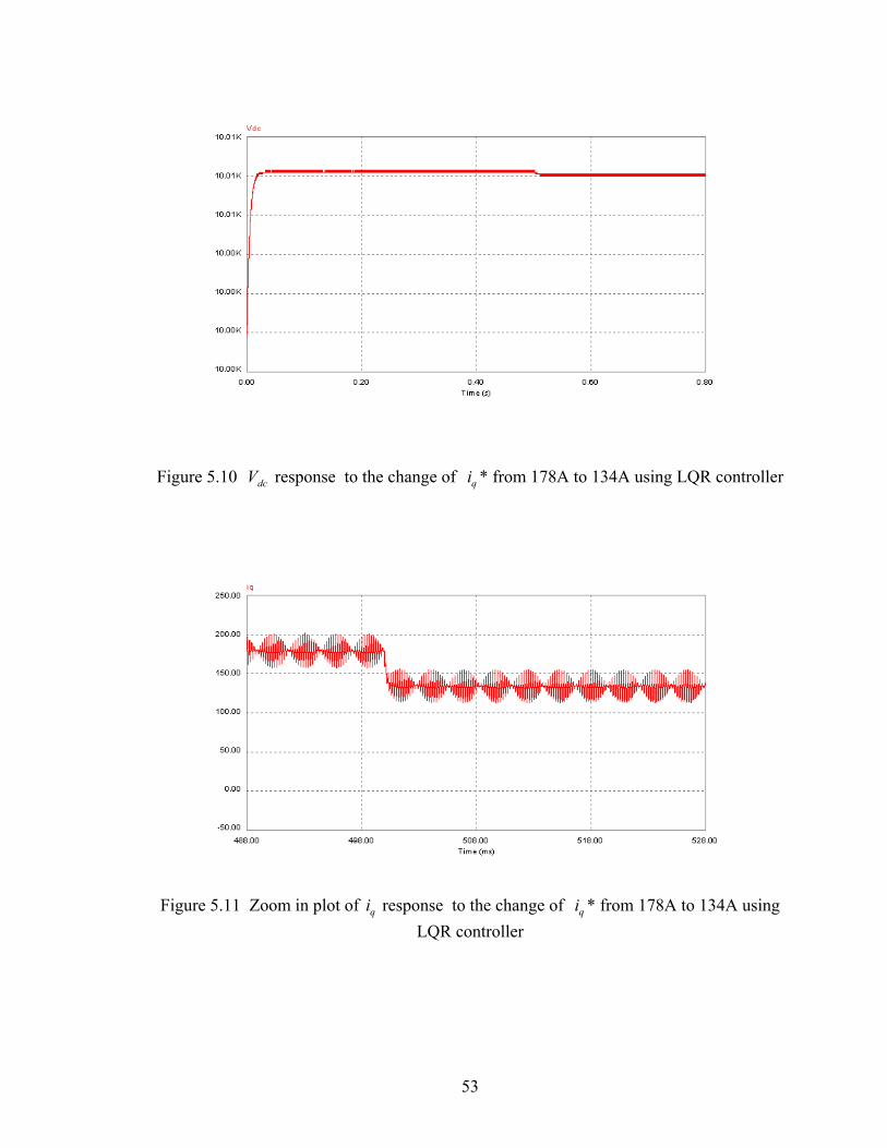
Figure 5.10 V response to the change of i * from 178A to 134A using LQR controller dc q
Figure 5.11 Zoom in plot of i response to the change of i * from 178A to 134A using q q
LQR controller
53
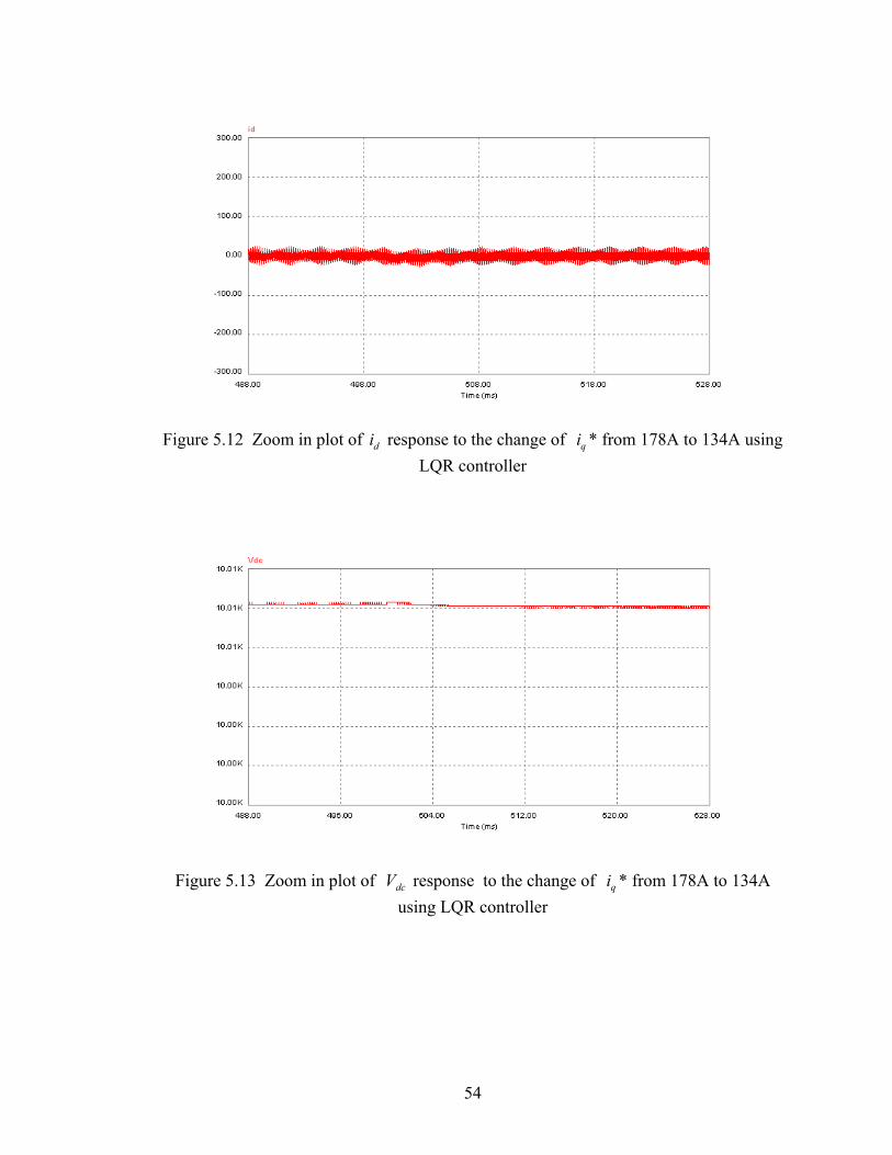
Figure 5.12 Zoom in plot of i response to the change of i * from 178A to 134A using d q
LQR controller
Figure 5.13 Zoom in plot of V response to the change of * from 178A to 134A
using LQR controller dc qi
54

CONCLUSION
We investigated the dynamic model of a typical STATCOM. Its characteristics
show that STATCOM is a nonlinear MIMO system with a control effort saturation
requirement. A linearization method can be used to deal with the nonlinear characteristic,
if given knowledge of operating point.
Based on the linearized mathematic model of STATCOM, full state feedback
controller was designed. The circuit validation showed that this control method is
effective and robust.
Two kinds of full state feedback controller (pole assignment and LQR) are
designed and compared to investigate a more suitable control method for STATCOM. It
was found that LQR controllers do not offer significant performance improvement to pole
assignment. However, as a design method the determination of state feedback gains are
easier to obtain using LQR method.
There are two topics of further interest noted in this thesis. One topic is to exam the
stability and controllability for different operating points. Such a study should lead to a
general of knowledge of (1) how various operating points affect the domain of attraction
of the equilibrium points and (2) how changes in operating points affect the
controllability of STATCOM. Another topic is considering the noise and disturbances
inherit in STATCOM. Here one may use robust & optimal control methods to determine
if improvements can be made in STATCOM performance.
55
REFERENCES
[1] L.Gyugyi, “Dynamic compensation of ac transmission lines by solid-state synchronous voltage sources.” IEEE Trans. Power Delivery, vol. 9, no. 2 pp.904-911, April 1994. [2] S. Mori et al., “Development of a large static var generator using self-commutated inverters for improving power system stability.” IEEE Trans. Power System, vol. 8, no. 1, Feb. 1993. [3] Schauder, C.; Gernhardt, M.; Stacey, E.; Lemak, T.; Gyugyi, L.; Cease, T.W.; Edris, A.; “Development of a ±100 MVAr static condenser for voltage control of transmission systems. ” IEEE Trans. Power Delivery, Vol. 10, Issue. 3, pp 1486 -1496, July 1995 [4] C. Schauder, M. Gernhardt and E. Stacey et al., “Operation of ±100 MVAR TVA STATCON.” IEEE Trans. Power Delivery, vol. 12 , no. 1, Oct. 1997. [5] John G. Vlachogiannis, “FACTS applications in load flow studies effect on the steady state analysis of the Hellenic transmission system”, Electric Power Systems Research, Vol. 55, Issue 3, Sept. 2000. [6] Papic, I.; Zunko, P.; Povh, D.; Weinhold, M. “Basic control of unified power flow controller .” IEEE Trans. on Power Systems, Vol.12, Issue.4, pp.1734 -1739 Nov. 1997 [7] FACTS & Definitions Task Force of the FACTS Working Group of the DC and FACTS Subcommittee, “Proposed terms and definitions for flexible AC transmission system.” IEEE Trans. Power Delivery, vol. 12 , no. 1, Oct. 1997. [8] Rao, P.; Crow, M.L.; Yang, Z. “STATCOM control for power system voltage control applications.” IEEE Trans on Power Delivery, Vol. 15 Issue: 4 , Oct. 2000 [9] Zhuang, Y.; Menzies, R.W.; Nayak, O.B.; Turanli, H.M, “Dynamic performance of a STATCON at an HVDC inverter feeding a very weak AC system.” IEEE Trans. on Power Delivery, Vol. 11 Issue: 2, pp.958 -964 April 1996 [10] Sensarma, P.S.; Padiyar, K.R.; Ramanarayanan, V.; “Analysis and performance evaluation of a distribution STATCOM for compensating voltage fluctuations.” IEEE Trans. on Power Delivery, Vol. 16 Issue: 2 , pp.259 -264 April 2001
56
[11] Arabi and P. Kundur, “Power oscillation damping control strategies for FACTS devices using locally measurable quantities”. IEEE Trans. on Power Systems. Vol. 10, Issue. 3, Aug.1995. [12] Garica-Gonzalez, P.; Garcia-Cerrada, “Control system for a PWM-based STATCOM.” IEEE Trans. on Power Delivery. Vol. 15 Issue. 4, Oct. 2000. [13] Arabi, S.; Hamadanizadeh, H.; Fardanesh, B.B. “ Convertible static compensator performance studies on the NY state transmission system.” IEEE Trans. on Power systems, Vol. 17, Issue: 3 , Aug. 2002 [14] K. R. Padiyar and K. Uma Rao, “Modeling and control of unified power flow controller for transient stability.” International Journal of Electrical Power & Energy Systems, Vol.21, Issue 1, January 1999. [15] Dong Shen; Lehn, P.W, “ Modeling, analysis, and control of a current source inverter-based STATCOM.” IEEE Trans on Power Delivery, Vol. 17, Issue: 1, pp. 266 -272 , Jan. 2002 [16] Anaya-Lara, O.; Acha, E, “Modeling and analysis of custom power systems by PSCAD/EMTDC .” IEEE Trans on Power Delivery, Vol. 17, Issue. 1, pp. 266 -272 Jan. 2002 [17] Lehn, P.W. “Exact modeling of the voltage source converter .” IEEE Trans. on Power Delivery, Vol. 17, Issue. 1, pp. 217 -222, Jan. 2002 [18] Fujita, H.; Tominaga, S.; Akagi, H. “Analysis and design of a DC voltage-controlled static VAr compensator using quad-series voltage-source inverters .” IEEE Trans. on Industry Applications, Vol. 32, Issue. 4, July-Aug. 1996 [19] Moran, L.T.; Ziogas, P.D. “ Joos, G.; Analysis and design of a novel 3-φ solid-state power factor compensator and harmonic suppressor system.” IEEE Trans. on Industry Applications, Vol. 25, Issue. 4, July-Aug. 1989 [20] N.Mohan, T. M. Undeland, and W.F. Robbins, Power Electronics: Converters, Applications and Design. New York: Wiley, 1989. [21] F. Lewis, Applied LQR and Estimation. Prentice hall, 1992. [22] G. Frankin, J, Powell, and M. Workman, Digital Control of Dynamic System. MA: Addison-Wesley, 1990. [23] P. C. Krause, Analysis of Electric Machinery. NY: McGraw-Hill Inc., 1986
57

58
BIOGRAPHICAL SKETCH The author was born in China. He received his B.S. degree and M.S. degree in Engineering from Huazhong University of Science & Technology, China. In the summer of 2001, the author enrolled at Florida State University. His research centered on the modeling and control of FACT devices & system. The author is a student member of IEEE.