Embed Size (px)
Citation preview

Investigation into Balancing of High-Speed Flexible Shafts by
Compensating Balancing Sleeves
James Grahame Knowles
A thesis submitted in fulfilment of the requirements of the University of
Lincoln for the degree of Doctor of Philosophy
2017
i
ABSTRACT Engineers have been designing machines with long, flexible shafts and
dealing with consequential vibration problems, caused by shaft imbalance
since the beginning of the industrial revolution in the mid 1800’s. Modern
machines still employ balancing techniques based on the Influence
Coefficient or Modal Balancing methodologies, that were introduced in the
1930’s and 1950’s, respectively.
The research presented in this thesis explores fundamental deficiencies of
current trim balancing techniques and investigates novel methods of flexible
attachment to provide a component of lateral compliance. Further, a new
balancing methodology is established which utilizes trim balance induced
bending moments to reduce shaft deflection by the application of
compensating balancing sleeves. This methodology aims to create encastre
simulation by closely matching the said balancing moments to the fixing
moments of an equivalent, encastre mounted shaft. It is therefore
significantly different to traditional methods which aim to counter-balance
points of residual eccentricity by applying trim balance correction, usually at
pre-set points, along a shaft.
Potential benefits of this methodology are initially determined by analysis of
a high-speed, simply supported, plain flexible shaft, with uniform eccentricity
which shows that near elimination of the 1st lateral critical speed, (LCS) is
possible, thereby allowing safe operation with much reduced LCS margins.
Further study of concentrated, residual imbalances provides several new
insights into the behaviour of the balancing sleeve concept: 1) a series of
concentrated imbalances can be regarded simply as an equivalent level of
uniform eccentricity, and balance sleeve compensation is equally applicable
to a generalised unbalanced distribution consisting of any number of
ii
concentrated imbalances, 2) compensation depends on the sum of the
applied balancing sleeve moments and can therefore be achieved using a
single balancing sleeve (thereby simulating a single encastre shaft), 3)
compensation of the 2nd critical speed, and to a lesser extent higher orders,
is possible by use of two balancing sleeves, positioned at shaft ends, 4) the
concept facilitates on-site commissioning of trim balance which requires a
means of adjustment at only one end of the shaft, thereby reducing
commissioning time, 5) the Reaction Ratio, RR (simply supported/ encastre)
is independent of residual eccentricity, so that the implied benefits resulting
from the ratio (possible reductions in the equivalent level of eccentricity) are
additional to any balancing procedures undertaken prior to encastre
simulation. The analysis shows that equivalent reductions of the order of
1/25th are possible.
Experimental measurements from a scaled model of a typical drive coupling
employed on an industrial gas turbine package, loaded asymmetrically with
a concentrated point of imbalance, support this analysis and confirms the
operating mechanism of balancing sleeve compensation and also it’s
potential to vastly reduce shaft deflections/ reaction loads.
iii
List of publications
Publications resulting from research presented in this
thesis
1. Mathematical development and modelling of a counter balance
compensating sleeve for the suppression of lateral vibrations in high
speed flexible couplings. ASME Turbo Expo San Antonio, TX, 3-7 June
2013; Paper number GT2013-95634. New York: ASME. Kirk A, Knowles
G, Stewart J, Bingham C, [117]
2. Theoretical investigation into balancing high-speed flexible-shafts, by
the use of a novel compensating balancing sleeve. IMechE Part C:
Journal of Mechanical Engineering Science 2013; Article No. 517376.
Knowles G, Kirk A, Stewart J, Bingham C, Bickerton R, [118]
3. Generalised analysis of compensating balancing sleeves with
experimental results from a scaled industrial turbine coupling shaft.
IMechE Part C: Journal of Mechanical Engineering Science - submitted
March 2017; Knowles G, Kirk A, Bingham C, Bickerton R, [119] -
PENDING
Patents
4. An apparatus comprising a shaft and a balancing device for balancing
the shaft. European Patent EP2703689A1. 2014. Knowles G, [123]
5. An apparatus comprising a shaft and a compensator balancing sleeve
for balancing the shaft. European Patent EP2806186A1. 2014. Knowles
G, [124]

iv
Acknowledgements
I would like to thank Siemens Industrial Turbomachinery Limited, Lincoln,
for past employment and their faith in funding this research.
A general thanks is due to my many friends and colleagues, too numerous
for individual acknowledgement, who helped me gain valuable experience
in all aspects of drive train dynamics and package design; but special
mention is due to: Mr. Steve Middlebrough, Mr. Herman Ruijsenaars, Dr.
Gordon Beesley, Mr. Alan Coppin, and in particular my friend and co-worker
Mr. Steve Atkinson, without whose help this germ of an idea would never
have flourished.
I am grateful to Professors Paul and Jill Stewart for their early
implementation and encouragement, Professor Ron Bickerton for his role of
Chief Engineer and listening post and a special thanks to my supervisor
Professor Chris Bingham for his very valuable advice and concise editorial
work.
I am also indebted to my work colleagues at the University of Lincoln, School
of Engineering, Technical Department and especially to my co-researcher
Mr. Antony Kirk, for his invaluable help during the rig build and validation
testing phases of this project.
Deserved thanks is also due to Mr. Dave Pemberton for his enduring
interest and stimulating many thought provoking discussions of my work
over many years.
Finally, but most importantly, sincere thanks is due to my wife Sally for
providing much needed support and encouragement.

v
Contents
Abstract ………………………………………………………...…………………i
List of Publications ………………………………………………...…………...iii
Acknowledgements …………………………………………………………….iv
Nomenclature …………………………………………………………………...ix
Glossary ………………………………………………………………………...xii
Chapter 1
1.1 Introduction ………………………………………………………………….1
1.2 Background …………………………………………………………………2
1.2.1 Historical Perspective ……………………………………………2
1.2.2 Balancing Machines ……………………………………………..7
1.2.3 Balancing Standards …………………………………………….9
1.2.4 Balancing Methods ………………………………….………….11
1.2.5 Lateral Critical Speed Margins …………………………...……17
1.2.6 Gyroscopic Action ………………………………………….……17
1.2.7 Instability Problems ………………………………………….….17
1.2.8 Rotating Coordinates …………………………………………..21
1.2.9 Complex vibration Analysis ……………………………………23
1.2.10 Estimating Residual Imbalance ……………………………...29
1.2.11 Fault Diagnosis ………………………………………………..30
1.2.12 Active-Balancing …………………..…………………………..31
1.2.13 Vibration Absorbers …………………………………………...35
1.3 Problem Statement – summarises points in background …………….36
1.4 Aims of this Research ………………………………………………........39
1.5 Main Contributions …………………………………………...…………...41
Chapter 2
2.1 Causes of Residual Imbalance ………………………………………….43
2.2 Trim Balancing Errors and Principle of Improvement …………………44
2.3 Theoretical Analysis of Balance Sleeve Compensation ……………...52
vi
2.4 Critical Speed Elimination ………………………………………………..59
2.5 Analytical Results …………………………………………………………60
2.6 Site Problem Simulation ……………………………………….…………67
2.7 Estimating Equivalent Shaft Eccentricity ……………………………….71
2.8 Preliminary Conclusions ………………………………….….…………..73
Chapter 3
3.1 Encastre Simulation …………………………………………..…………..75
3.2 Compensated Critical Speeds …………………………………………..81
3.3 Elimination/ Nullification of Compensated Critical Speed …………….87
3.4 Encastre Points of Conversion …………………………………………..89
3.5 Practical Possibility of Critical Speed Elimination ……………………..92
3.6 Sensitivity Study ……………………………………….………………….93
3.7 Preliminary Conclusions ………………….………….…………………..95
Chapter 4
4.1 Generalised Analysis of Concentrated Imbalances …………………...96
4.2 Theoretical Analysis ………………………………………………………96
4.3 Eliminating/ Nullifying the Impact of the 1st Critical Speed ………….108
4.4 Encastre Simulation ……………………………………………………..111
4.5 Compensated Critical Speed Elimination ……………………………..115
4.6 Practical Implications ……………………………………………………116
4.7 Additional Elimination/ Nullification of the 2nd Critical Speed ……….118
4.8 General Imbalance Distribution ………………………………………..119
4.9 Analytical Results: site equivalent model with a single offset
imbalance …......................................................................................120
4.10 Preliminary Conclusions ……….……………………..……………….123
vii
Chapter 5
5.1 Shaft End Reaction Loads ……………………………………………...124
5.1.1 Simply Supported Shafts ……………………………………..124
5.1.2 Encastre Mounted Shafts …………………………………….125
5.2 Shear Force Reaction Ratio/ Equivalent Level of Shaft
Eccentricity ……................................................................................127
5.3 Applicability of Shear Force Reaction Ratio ………………………….128
5.3.1 Plain Shafts with Concentrated Imbalances ………………..128
5.3.2 Shaft Mounted Discs ………………………………………….132
5.4 Balancing Sleeve Design …………………………………………...….136
5.5 Effect of Double Encastre Mounting on Higher Order Critical
Speeds ……………………………………………………………………138
5.6 Simulation Ratio………………………………………………………….141
5.7 Preliminary Conclusions ……….……………………………………….148
Chapter 6
6.1 Test Rig Design …………………………………………………..……..152
6.2 Instrumentation …………………………………………………………..153
6.3 Test Coupling Shaft ……………………………………………………..154
Chapter 7
7.1 Compensating Balancing Sleeve Design ……………………………..158
7.2 Double Encastre Beam …………………………………………………162
Chapter 8
8.1 Test Requirements ………………………………………………………167
8.2 Test Procedure ……………………………………………………….….167
8.3 Test Results …………………………………………………………......172
8.3.1 General Measurement Orientation ………………………….172

viii
8.3.2 Test Data ……………………………………………………….175
8.3.3 Bearing Reaction Loads ……………………………………...182
8.3.4 Test and Theoretical Comparisons ………………………….183
8.4 Preliminary Conclusions …………………………………….………….191
Chapter 9
9.1 Conclusions ………………………………………………………………194
References …………………………………………………………..…….201
Appendices
Appendix A ………………….………………………………………………..212
Appendix B ……………………………………………………………………215
Appendix C …………………………………………………………………...216
Appendix D …………………………………………………………………...217
ix
Nomenclature
General Analysis
iA0 ,Ai, iB0 , Ci,Di,G,H,M,N,P,Q,b = Parameters substitutions
Parameter Suffixes: e = encastre shaft
un = uniform eccentricity
con = concentrated imbalance
ss = simply supported
en = encastre mounted
a,f = Eccentric zone end positions (m)
BM= Shaft bending moment at point x
ic = Eccentricity of balance sleeve mass ( m)
CF = Centrifugal force (N)
discCF = Disc centrifugal Force (N)
balCF = Balance centrifugal Force (N)
e = Eccentricity of shaft (m)
e = Euler’s number
disce Disc eccentricity (m)
bale Balance eccentricity (m)
E = Young’s Modulus (N/m^2)
I = 2nd Moment of area in bending (m^4)
k = Concentrated imbalance coefficient
iK = Balance sleeve stiffness (N/m)
i, = Shaft length (m)
iL = Balance sleeve length (m)
L = Non-dimensional sleeve length
im = Balance sleeve mass (kg)
fiM = Encastre system fixing moment (Nm)
x
iM 0 = Balance sleeve moment applied to shaft (Nm)
xM = Balance sleeve moment applied to shaft at point x (Nm)
sM = Shaft mass (kg)
discM = Disc mass (kg)
balM = Balance mass (kg)
Mp = Concentrated zone mass (kg)
Mu = Equivalent additional mass (kg)
r = Shaft radial deflection (m)
iR = Parameters of shaft radial deflection (m)
ilR = Parameter derivatives of shaft radial deflection
ii Rrr ,, = Laplace displacement derivatives
R = Radius of rotation of equivalent additional mass Mu (m)
eiR = Reaction load at shaft ends (N)
eR = Non dimensional reaction load
s = Laplace Transform operator
SFv = Vertical Shear Force
balS = Balance stiffness (N/m)
shaftS = Shaft stiffness (N/m)
balS = Balance Stiffness (N/m)
W = Lateral load applied to a beam/ shaft
x = Reference point position from shaft end (m)
iy = Balance mass displacement from rotation axis (m)
iY = Balance sleeve deflection (m)
= Rotational speed (rad/s)
critbal_ = Balance critical speed (rad/s)
critshaft_ = Shaft critical speed (rad/s)
xi
crit = Critical speed (rad/s)
Compensating Sleeve Design
A = Spar cross sectional area (m^2)
bowBM _ = Spar radial bending moment (Nm)
deflBM _ = Spar vertical bending moment (Nm)
resBM _ = Spar resultant bending moment (Nm)
max_f = Maximum bending stress (N/m^2)
h = Height of spar centroid above X – X (m)
ccI = Spar moment of inertia through centroid (m^4)
xxI = Spar moment of inertia about X - X (m^4)
sleeveI = Sleeve bending moment of inertia (m^4)
M = Fixing moment of double encastre beam (m)
1M = Spar 1st moment of area about X - X (m^3)
2M = Spar 2nd moment of area about X - X (m^4)
iR = Spar sectional radius (m)
R = Reaction load of double encastre beam (m)
u = Displacement of double encastre beam (m)
i = Spar angular position (rad)
fibrey = Distance of extreme fibre in bending (m)

xii
Glossary
ABB Automatic Ball Balancer
API American Petroleum Institute
AGMA American Gear manufacturers Association
BW Backward Whirl
CF Centrifugal Force
CR Compensation Ratio
DAVC Direct Active Vibration Control
DOF Degree of Freedom
FEA Finite Element Analysis
FW Forward Whirl
ISO Institutional Organisation for Standardisation
GE General Electric
LCS Lateral Critical Speed
LHS Left Hand Side
N Number of modal balance planes
N + 2 Number of modal + rigid body balancing planes
pk – pk Peak to Peak
PT Power Take-Off
RHS Right Hand Side
RR Reaction Ratio
SR Simulation Ratio
TDC Top Dead Centre
TP Test Procedure
2-D, 2.5-D, 3-D Number of analysis planes considered in FEA
1
Chapter 1
1.1 Introduction
The investigation presented in this thesis was initiated by the need for
controlling shaft vibration issues encountered in Gas Turbine (GT) driven
Mechanical Drive Packages for the Oil and Gas market. Such units are
usually required to pump liquid or gas, for utility purposes, over 100’s of
kilometres and must be able to operate over a wide speed range in order to
provide the necessary performance flexibility to maintain a high overall
operating efficiency.
However, it has been observed that in some instances it has been extremely
difficult, and often impossible to dynamically balance the GT shafts across
the required operating speed range because the phase vector of the bearing
load was changing with respect to operating speed. Specifically, drive trains
could be readily balanced at relatively low operating speeds, but with a new
angular position of the load vector it was incorrectly balanced at higher
operating frequencies, or vice versa.
In some cases the vector change is seen to approach 180°, indicating that
the drive train would have traversed a critical speed, between the low and
high speed operating points. However, dynamic analysis showed this not to
be the case.
It is notable that such problems appear more acute on packages where the
drive coupling, between the driver and driven units, was longer than
standard, or had torque spacers incorporated as part of the assembly. In
both cases the shaft flexibility is increased and this led to a hypothesis that
shaft deflection could be an alternative cause of angular change of the
vector. In turn, this has led to the proposition of an improved balancing
mechanism, the compensated balancing sleeve [120,121,122,123,124],
2
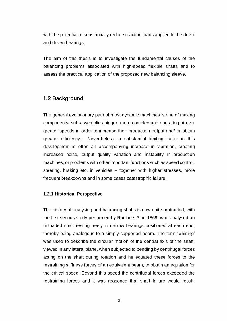
with the potential to substantially reduce reaction loads applied to the driver
and driven bearings.
The aim of this thesis is to investigate the fundamental causes of the
balancing problems associated with high-speed flexible shafts and to
assess the practical application of the proposed new balancing sleeve.
1.2 Background
The general evolutionary path of most dynamic machines is one of making
components/ sub-assemblies bigger, more complex and operating at ever
greater speeds in order to increase their production output and/ or obtain
greater efficiency. Nevertheless, a substantial limiting factor in this
development is often an accompanying increase in vibration, creating
increased noise, output quality variation and instability in production
machines, or problems with other important functions such as speed control,
steering, braking etc. in vehicles – together with higher stresses, more
frequent breakdowns and in some cases catastrophic failure.
1.2.1 Historical Perspective
The history of analysing and balancing shafts is now quite protracted, with
the first serious study performed by Rankine [3] in 1869, who analysed an
unloaded shaft resting freely in narrow bearings positioned at each end,
thereby being analogous to a simply supported beam. The term ‘whirling’
was used to describe the circular motion of the central axis of the shaft,
viewed in any lateral plane, when subjected to bending by centrifugal forces
acting on the shaft during rotation and he equated these forces to the
restraining stiffness forces of an equivalent beam, to obtain an equation for
the critical speed. Beyond this speed the centrifugal forces exceeded the
restraining forces and it was reasoned that shaft failure would result.
3
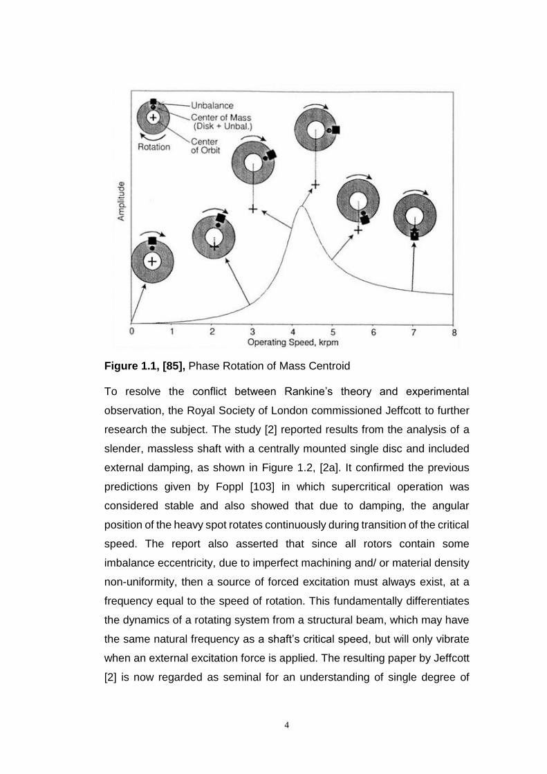
However, by not being aware that phase rotation of the mass centroid
occurs about the geometric centre of the shaft, during transition through a
critical speed, see Figure 1.1, [85], it was erroneously concluded at the time
that operating beyond this speed was impossible.
Nevertheless, following this study a steam turbines was developed that
could operate above the 1st critical speed, by De Laval in 1883 and by
Parsons in 1884, [5], and hence some empirical engineering knowledge
about self-balancing mechanisms existed whereby at super-critical speeds
the “shaft again runs true”. In 1895, an analysis of an undamped rotor by
Foppl [103] showed that the heavy side, or heavy spot, of an unbalanced
disc migrates outwards when rotation is below the critical speed and that it
migrates inwards, thus lessening the imbalance, when operated above the
critical speed. Moreover, Dunkerley [1] in 1894 published experimental
results of the critical speeds of numerous slender shafts, loaded with a
variety of differently positioned pulley wheels, as was in common use in the
cotton mills at the time, which further supported the above theories.
4
Figure 1.1, [85], Phase Rotation of Mass Centroid To resolve the conflict between Rankine’s theory and experimental
observation, the Royal Society of London commissioned Jeffcott to further
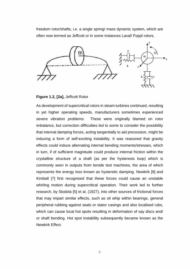
research the subject. The study [2] reported results from the analysis of a
slender, massless shaft with a centrally mounted single disc and included
external damping, as shown in Figure 1.2, [2a]. It confirmed the previous
predictions given by Foppl [103] in which supercritical operation was
considered stable and also showed that due to damping, the angular
position of the heavy spot rotates continuously during transition of the critical
speed. The report also asserted that since all rotors contain some
imbalance eccentricity, due to imperfect machining and/ or material density
non-uniformity, then a source of forced excitation must always exist, at a
frequency equal to the speed of rotation. This fundamentally differentiates
the dynamics of a rotating system from a structural beam, which may have
the same natural frequency as a shaft’s critical speed, but will only vibrate
when an external excitation force is applied. The resulting paper by Jeffcott
[2] is now regarded as seminal for an understanding of single degree of
5
freedom rotor/shafts, i.e. a single spring/ mass dynamic system, which are
often now termed as Jeffcott or in some instances Laval/ Foppl rotors.
Figure 1.2, [2a], Jeffcott Rotor As development of supercritical rotors in steam turbines continued, resulting
in yet higher operating speeds, manufacturers sometimes experienced
severe vibration problems. These were originally blamed on rotor
imbalance, but correction difficulties led to some to consider the possibility
that internal damping forces, acting tangentially to aid precession, might be
inducing a form of self-exciting instability. It was reasoned that gravity
effects could induce alternating internal bending moments/stresses, which
in turn, if of sufficient magnitude could produce internal friction within the
crystalline structure of a shaft (as per the hysteresis loop) which is
commonly seen in outputs from tensile test machines, the area of which
represents the energy loss known as hysteretic damping. Newkirk [8] and
Kimball [7] first recognised that these forces could cause an unstable
whirling motion during supercritical operation. Their work led to further
research, by Stodola [5] et al, (1927), into other sources of frictional forces
that may impart similar effects, such as oil whip within bearings, general
peripheral rubbing against seals or stator casings and also localised rubs,
which can cause local hot spots resulting in deformation of say discs and/
or shaft bending. Hot spot instability subsequently became known as the
Newkirk Effect.
6
Campbell [6], (1924), investigated vibrations resulting currently from
General Electric, GE, steam turbines and developed a method for plotting
critical speeds and lines of synchronous excitations against operating
speed, with their intersections highlighting points of whirling resonance—
now widely known as Campbell Diagrams. During this period of rapid
analytical development many accompanying bench tests were performed to
measure the internal friction characteristic of various materials. Kimball,
Lovell et al, [7] employed cantilever shafts with over-hung masses
suspended from shaft end bearings, so that vertical gravity forces induced
sinusoidal, once per revolution, bending stresses as the shaft rotated. The
results showed that the hanging mass was always deflected to one side by
a tangential damping force and its angular displacement was independent
of the shafts rotational speed, but proportional to its vertical deflection. From
bending stress/ strain relationships, the authors were able to relate the
damping energy/ work done per cycle and hence a material/ damping loss
factor to the angular off-set.
In 1933 Smith [14] analysed a rotor system with internal viscous damping
and proved that without any external damping the system became unstable
at the 1st critical speed. This point is called the instability threshold as the
internal viscous damping had a stabilising effect up to this point, i.e. at
subcritical speeds. Further, the presented formulae predicted that the
threshold spin speed varied with the ratio of the internal to external damping.
Other researchers [10-12] later confirmed these conclusions by differing
methods and also showed that by including external damping the threshold
of instability can be increased beyond the critical speed. By analysing the
system using rotational coordinates and assuming isotropic supports, i.e.
orthogonal coordinates fixed to the shaft, so that shaft forces/ moments
seen from this perspective are independent of rotational speed and only the
stationary environment is seen to rotate, reduces the mathematical
complexity and simplifies the solution. This concept enhanced the
understanding of forward and backward whirl, where a rotor spins about its
7
geometric centre due to the machine’s driving torque, but also rotates,
positively or negatively, about its bearing centres, (usually offset from the
geometric centre by shaft deflection), to produce a whirl velocity. It was
shown that the tangential direction of the internal damping force is
proportional to the difference in these speeds and changes direction at the
critical speed when they are equal. Instability results at supercritical speeds
when the tangential force due to internal damping exceeds the equivalent
external damping force.
It was also recognised that one of the main causes of internal damping came
from interface friction within rotor joints due to flexing as cyclic bending
occurred. Special test rotors were made to investigate shrink fits, in
particular, as these were commonly used in turbine and compressor design.
Robertson [13] et al concluded that axial fits should be short and as tight as
possible, without exceeding the yield strength of the material and that if a
long fit was required, it should be relieved in its centre to reduce the contact
area. He also asserted that any friction which tends to limit a shaft’s
deflection will add to internal damping, e.g. as occurs between the teeth of
gear couplings or the flexible laminations within disc couplings. But note
must be made of the fact that different mechanisms cause different damping
effects; for instance, mechanical rub produces a ‘stick-slip’ motion resulting
in Coulomb damping, whereas hydrodynamic forces produce the classical
viscous damping [58].
1.2.2 Balancing Machines
Separately to this fundamental research, manufacturers and engineers
developed various methods of reducing the residual imbalance in rotating
components and assemblies by attempting to correct the centre of mass
eccentricity. In the late 1800’s and early 1900’s this was largely by trial and
error, by placing a rotor horizontally on knife edges, using the ‘roll-off’
method. Mass was either added, or removed, in appropriate places, until

8
there was no tendency for the rotor to rock backwards or forwards or for an
induced force to produce a cyclic rolling motion. This important work was
performed by skilled fitters, but it could take 3 to 4 weeks, using a step by
step approach, to balance a large steam turbine rotor assembly.
Consequently, balancing machines were being developed to provide more
accuracy and to speed up the process. Carl Schenck [21] commissioned
such a machine in 1908 and later concluded a worldwide licensing
agreement, in 1915, for a much improved, pendulum mounted machine,
patented by Franz Lawaczeck, publication number, US1457629A.
The 1940’s began to see electronic systems/sensors incorporated into
balancing machine designs to measure both the magnitude and vector
position of centrifugal forces imposed by unbalance, usually in two planes
of the shaft axis. Special purpose machines were designed to meet the
varying requirements of different industries [48,62], for example machine
tool spindles required a very high degree of balance – equivalent
eccentricity, e, of less than 0.000002 in, whereas motor car wheels only
require an eccentricity, e, of less than 0.01 in. The designs either required
the mounting of the test rotor in flexible/ soft or rigid/ hard bearing pedestals,
so that the balancing speed of the rotor had a 4 to 5 times separation margin
with the natural frequency of the supporting structure; this minimised
response changes due to speed and ensured proportionality between the
measured rotor response and its imbalance. For soft bearing designs, the
test speed is usually well above the pedestal natural frequency, therefore
stiffness and damping forces are small compared with the excitation and
inertia forces and can be neglected so that shaft unbalance is directly
proportional to pedestal displacement. In the case of hard bearing
machines, the test speed is well below the pedestal natural frequency, so
that damping and inertia forces are neglected and shaft unbalance is directly
proportional to the pedestal reaction force. The choice of pedestal design
and its test running speed was therefore often, by practical necessity,
determined by the size/ mass of the rotor. Measurements were generally

9
made using electro-mechanical, moving coil transducers fitted to the
bearing pedestals. Two types of systems were commonly used to measure
or indicate the phase angle of the unbalance vector; either a stroboscopic
light, triggered by the sinusoidal transducer outputs was used to light up the
high point on a series of index numbers fastened on to the circumference of
the rotor shaft, or the wattmeter method. In this case the output from a sine/
cosine wave generator, (2 electrical pick-up brushes at right angles,
contacting a shaft mounted, circular resistance element), is fed into one side
of a wattmeter and the vibration transducer output is fed into the other. Since
a wattmeter only produces an output deflection when the two input coils
have signals of the same frequency, both the unbalance magnitude and
phase angle can be determined mathematically from the two outputs
corresponding first to the sine and second the cosine generated inputs.
The 1950’s saw balancing times and costs further reduced by the integration
of metal removal accessories to high volume balancing machines, so that
mass correction could be made during the measuring procedure, without
the need to transfer the rotor to a separate machine.
1.2.3 Balancing Standards
However, even after undergoing a good balancing procedure, a perfect
balance could never be achieved and the necessity to determine an
appropriate level of balance quality, dependant on the type of application,
became apparent and led to the introduction of several international
standards whose aims was not only to produce a set of balance grades/
levels that would be economically functional, but also to standardise on
terminology, measuring procedures and units of measurements etc. in order
to minimise disputes between operators and venders.
A commonly employed standard is The International Organisation for
Standardisation, ISO 1940/1, Balancing Quality Requirements of Rigid
10
Rotors [17,18], which reflects usage principally in metric systems and has
been adopted by British, German and American National Standards; it
categorises rotors, based on world wide experience, according to their type,
mass, and maximum service speed, into a quality grade, G. Its
corresponding number relates to the allowable level of vibration, mm/sec,
measured on the bearing housing at the service speed and is the product
of specific unbalance, (unbalance, g,mm/ rotor mass, kg) and the maximum
angular velocity, rad/sec. Consequently, G is related to permissible residual
unbalance measured in g.mm and allowable mass centre displacement, i.e.
eccentricity, measured in microns, µm. This standard is based primarily on
single components—for assemblies, it requires that the unbalances of
component parts shall be added vectorially, taking account of expected
unbalances resulting from assembly inaccuracies whilst also noting that
further assembling positions may be different. ISO 5406-1980, The
Mechanical Balancing of Flexible Rotors [22], classified flexible rotors into
groups according to their balance requirements, established assessment
methods for final unbalance and provided guidance on the establishment of
balance grades. Rotors are classified to indicate which can be balanced by
normal, modified rigid balancing techniques or which require some method
of high-speed balancing. The standard is not an acceptance specification,
but an aid to avoiding gross deficiencies, exaggerated or unattainable
requirements.
The American Gear Manufacturers Association, AGMA 515 and 9000,
Flexible Couplings – Potential Unbalance Classification [16], reflects usage
principally in inch systems and is based on similar principles to ISO, but its
method relates directly to flexible coupling assemblies. It specifies the
unbalance in terms of a Balance Class Number, according to operating
speed and coupling weight, representing the maximum displacement of the
principal inertia axis, at specified balance planes, in micro-inches, µ-in.
11
More specifically, for the petroleum, chemical and gas industries, the
American Petroleum Institute, API, which is of particular importance for the
application sector of this thesis, has issued a number of design standards
and recommended practices [15,19,20], which specify methods/ vibration
limits for lateral dynamic analysis and very detailed balancing methods for
couplings. These apply both to components and assemblies, with
repeatability checks and specify unbalance limits, in inch and metric units,
dependent on the proportionate mass at a balance plane and its maximum
operating speed.
As an acknowledgement of the importance and difficulty of obtaining/
maintaining conditions of good balance, standards were also introduced that
specify means of evaluating shaft and casing vibration, for monitoring,
warning and shutting down machines, before serious damage occurred. ISO
7919-4 2nd Edition 2009-10-01 Mechanical Vibration – Evaluation of
machine vibration by measurements on rotating shafts: Part 4 Gas turbines
sets with fluid-film bearings [23] and ISO 10816-4 2nd Edition 2009-10-01
Mechanical Vibration – Evaluation of machine vibration by measurements
on non-rotating shafts : Part 4 Gas turbines sets with fluid-film bearings [24],
are two such examples.
1.2.4 Balancing Methods
Concurrent to the introduction of balancing standards were advancements
in dynamic analysis and balancing methodology. All balancing techniques
rely on making mass corrections in various axial positions along a shaft, but
since it is unlikely that addition or reduction of mass can take place directly
in the same plane as the inherent unbalance, special balancing planes are
usually employed for this purpose, but their position is dependent on the
rotor type. Rotors are generally classified for balancing purposes as being
either rigid or flexible. Since all rotors are known to be flexible if operated at
a high enough speed, the rigid definition determines that no significant
12
bending deformation must occur and that shafts rotate about their centre
lines, which shall remain straight, although bearing pedestals may deflect.
This generally limits the maximum operating speed to be less than 75% of
its lowest flexural critical speed [32]. Rigid types are by far the easiest to
balance since, even if mounted on flexible pedestals, there are no more than
two modes of vibration/ critical speeds. Translator/bounce, where both ends
of the rotor appear to go up and down together in a circular or elliptical orbit,
resulting from a unidirectional, imbalance distribution, and a conical/ tilt
mode, where motion of the ends are in anti-phase, resulting from an
unbalance moment—caused by non-directional uniformity of the unbalance
force vectors or gyroscopic effects. Hence, only two balancing planes are
required to accomplish a state of good balance when operating near either
of the critical speeds and these are generally positioned close to the
pedestals for maximum effect.
Due to the greater difficulty of balancing flexible rotors they have generated
much more research and produced two primary categorisations of methods
for balancing them; known as the influence coefficient method and modal
balancing.
The influence coefficient method was proposed by Thearle [50] in 1934,
primarily for large electrical alternators weighing over 100 tons, and hence
far too big for balancing machines. The technique considers single and two
plane balancing of rotors at a given speed by individually placing trial
weights at either end of the machine and measuring the response at each
end relative to the prior response due solely to the rotor’s residual
unbalance. Assuming a linear system, vector algebra is used to determine
vector operators or influence coefficients that are considered fundamental
characteristics of the machine, from the measured change in vibration
amplitude and phase angle due to the additional trial weights. These are
then used to calculate the required magnitude and angular position of the
correcting masses needed to balance the rotor. The complexity of the

13
method is increased when applied to multi-mass rotors, which typically
require N trial runs for N balance planes—where response measurement is
needed at each of the balance planes. More recently the use of matrix
analysis and specialised computer programmes to determine the influence
coefficients/ final trim balance corrections [48] are used. For instance,
Goodman [55] in 1964 developed a weighted least squares calculation
procedure to optimise the test data from multiple speeds and measuring
locations. However, the use of trial weights does not accommodate other
possible causes of unbalance, such as moment unbalance, caused by
skewed discs, or shaft bow – caused by internal stresses induced during
manufacture; hence it is possible that a good balance condition only applies
at speeds close to the test speed and the shaft is unbalanced at other
speeds.
The second method, modal balancing, is based on a detailed mathematical
model of the system from which a relationship between the shaft
displacement and the forcing function, for each of the critical speeds within
the operating range of interest can be estimated. For analysis purposes two
models have generally been employed: one where the rotor is considered
as a series of point masses and the second where the shaft is treated as a
continuous elastic body. The latter method, pioneered by Bishop [26],
Gladwell [25,29] and Parkinson [32,33] developed a general unbalance
distribution in terms of modal unbalance eccentricities. Using classical
vibration theory and assuming simple supports, the critical speeds
correspond to flexural natural frequencies of equivalent non-rotating beams
with distinct deflexion shapes corresponding to particular modes of
vibration—a simple bow for the 1st mode and a horizontal ‘S’ for the 2nd etc.
Consequently, the components of each vibration mode are dependent on
the particular parameters relating to that mode and the concept of
orthogonality applies so that the differential equations of motion are
independent of any cross-coupled forces or moments that may be present
in other planes. It was claimed [32,48] that the unbalance distribution along

14
a shaft is not confined to any one axial plane, but that a modal unbalance
distribution does lie in such a plane, which may vary from mode to mode.
Hence, eccentricity is represented as a shaft distribution that includes
parameter coefficients dependent on the mode/ natural frequency index
number, 1st, 2nd 3rd etc. and presented as a mathematical series formulation
that is integrated over the shaft length to establish the resultant unbalance
for the mode.
With increasing computing power, the modelling of rotors as a series of
elements/ point masses, gained prominence, allowing detailed analysis of
much greater complexity, but producing systems with very large numbers of
natural frequencies/ degrees of freedom, DOF’s. Numerical solutions for this
type of modelling are generally obtained by finite element analysis, (FEA),
and such programs are today capable of solving extremely large matrix
equations containing many thousands of elements. With the availability of
such tools the desire for greater accuracy ensued and modifications to the
method of modal balancing were reported. Kellenberger’s [52] 1972
contribution studied the N modal planes of balancing proposed by Bishop
et al, and also an N+2 method, which balanced the rigid body modes first,
followed by the N flexible modes. The paper reported that the second
method produced a greater degree of balancing accuracy. Racic and
Hidalgo [45] in their 2007 review of practical balancing concluded that “there
is no better or worse balancing method, only the more or less economical”.
Nevertheless, in many cases the balancing process can be costly and time
consuming, requiring several start-ups of the machine etc., which prompted
researchers to investigate methods of balancing without trial weights [99]. It
was reasoned that trial runs could be numerically simulated providing that
the modelling of the rotor system is sufficiently accurate. An initial
methodology, without damping, was proposed by Hundal and Harker [53]
and later refined using more generalised analysis by Morton [31] and others,
in the mid 1980’s, to include damping, that also made allowance for different
15
bearing characteristics from the vibration data obtained during normal
operation runs.
Due to readily available computing power and sensors, high speed/
response machine control software was frequently being installed on
machines to protect bearings. This required the use of bearing proximity
probes which were typically installed in bearing casings to measure shaft
radial displacement, at any two coplanar positions, phased 90º apart,
together with a shaft position sensor, (key phaser), which allowed the shaft
orbit, within the bearing clearance to be monitored. Software then provided
initial warnings and then if necessary initiated unit shut downs if the
percentage of bearing clearance was considered dangerously low. This new
facility also helps during site commissioning, by enabling production of
frequency response curves, bode diagrams and polar plots to be made,
during run-up and down tests. Hence, checks on actual critical speeds,
damping ratios and bearing loads can be made so as to feed direct
measurements to balancing processes.
Some researchers [44] made use of this additional data and incorporated
complex algebra into their analysis and subsequent balancing programmes
to present the x and y vector information as single modal parameter
components, of eccentricity, unbalance mass/ centrifugal force, shaft
deflection and bearing reaction load, etc. This real data allowed calibration
of FEA models and provided increased analytical accuracy. As a result there
followed several publications [34,41,43,51,54] of time saving
methodologies, to enable balancing, for example, with a single trial weight
test, or a single vibration transducer, or balancing without any trial runs at
all. Further, Garvey [28] et al proposed utilising knowledge of the expected
machine characteristics to introduce cost functions, based on the probability
distribution of certain parameter variability or uncertainty, such as support
stiffness. The authors reported, for example, elastomer supports whose
characteristics change with temperature and age; and also noted that some
16
vibration, say at bearing pedestals, might be more tolerable than other
synchronous vibration, at positions where stator/ rotor clearances are very
low. By analysing the cost functions applicable to the machine in question,
the authors were able to combine them to produce a weighted sum factor,
which is then used to determine the required unbalance correction by
minimising the worst possible cost.
The design of modern gas turbines requires faster, lighter engines utilising
the very latest manufacturing techniques to produce longer, thinner and
more flexible shafts. This has led to an increasing number of machines
required to operate super critically and has spawned the requirement for
economic procedures of obtaining good balance at these speeds. A
practical procedure, suggested by Hylton [30] in 2008, demonstrated that
by sharing the required balance correction between 3 balance planes, a
good compromised state of balance can be achieved using only low speed
balancing, which enabled machine operation at both sub- and super-critical
speeds. The analysis of an assumed sinusoidal unbalance distribution and
shaft deflection concluded that for a first balancing run, half of the resulting
balance correction should be made at a central balance plane, with the
remaining correction shared between the shaft end planes. A second
balancing run is then made and the resulting balance correction shared
solely by the end planes. The shaft is then considered balanced. This
procedure proved successful on a number of engines used in the aerospace
industry [30]. FEA analysis of other unbalance/ shaft geometric distributions
produced other shape functions, which required a slightly different position
for the 3rd balancing plane, but the same procedure remains applicable.
A good overview of well known balancing methods, including case histories
of difficult balancing problems, is provided by Feese [67] and Grazier, 2004.
17
1.2.5 Lateral Critical Speed Margins
The above balancing procedures came about due to industry’s ability to
dynamically analyse very complex rotor shafts, usually by the use of FEA
software; initially 2 dimensional, (2D), then 2.5D and now 3D. However, the
use of such tools requires a greater level of engineering expertise than is
traditionally available, i.e. rotor dynamic specialists. Hence, it remains
common practice for lateral analysis to be simplified by being confined to
individual driver and driven machines, as opposed to modelling the full drive
train; since the flexible coupling between them is assumed to have ‘moment
release’ and to act as a lateral hinge. However, this simplification makes
assessing the critical speeds less accurate and therefore requires large
margins between the maximum operating speed and the lateral critical
speed, (LCS), for safe operation; typically 150%, as required by most API’s
[15,19,20]. This requirement is particularly problematic for
manufacturers/users of high speed couplings (as highlighted by Corcoran
[27] in 2003), since although the critical speed of a coupling is calculated as
an individual item, based solely upon its bending stiffness, in reality its true
value also depends on the neighbouring stiffness’s of the driver and driven
units. It is suggested that the 150% margin is only suitable where such
stiffness’s are extremely high, and a two times or higher margin should
generally be used in the absence of a full train FEA analysis.
1.2.6 Gyroscopic Action
The importance of gyroscopic action on large discs and its contribution to
critical speeds was well known and the general problem of free vibration of
a single rotor on a light shaft had been considered by Timoshenko [61],
Stodola [5], Green [56]. It was shown that gyroscopic action produced
moments were proportional to the rate of change of the angle of tilt, known
as the precession velocity, and acted orthogonally at 90º to the lateral
displacement of the shaft, thereby resulting in moments that made positive
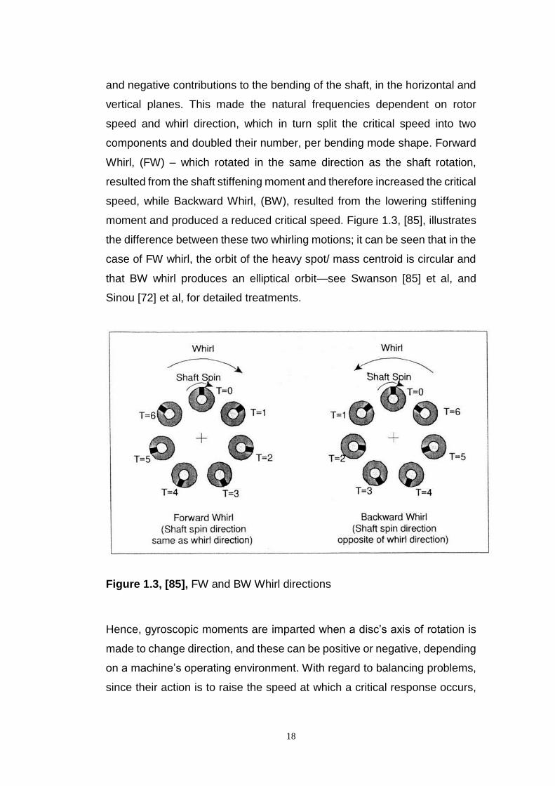
18
and negative contributions to the bending of the shaft, in the horizontal and
vertical planes. This made the natural frequencies dependent on rotor
speed and whirl direction, which in turn split the critical speed into two
components and doubled their number, per bending mode shape. Forward
Whirl, (FW) – which rotated in the same direction as the shaft rotation,
resulted from the shaft stiffening moment and therefore increased the critical
speed, while Backward Whirl, (BW), resulted from the lowering stiffening
moment and produced a reduced critical speed. Figure 1.3, [85], illustrates
the difference between these two whirling motions; it can be seen that in the
case of FW whirl, the orbit of the heavy spot/ mass centroid is circular and
that BW whirl produces an elliptical orbit—see Swanson [85] et al, and
Sinou [72] et al, for detailed treatments.
Figure 1.3, [85], FW and BW Whirl directions
Hence, gyroscopic moments are imparted when a disc’s axis of rotation is
made to change direction, and these can be positive or negative, depending
on a machine’s operating environment. With regard to balancing problems,
since their action is to raise the speed at which a critical response occurs,
19
i.e. when shaft rotation coincides with a natural frequency having FW whirl,
then knowledge of their contribution means the safe operating margins can
often be increased.
Several studies made use of differing analytical techniques to solve the
added complexity of gyroscopic action. Aleyaasin [82] et al made use of
advanced computer capability to manipulate large matrix equations, a
transfer matrix approach, as used in control theory, in which a series of
flexible, distributed elements, connected together by rigid discs, forming
lumped elements, were used to create a matrix model of a rotor. Laplace
transforms are then applied to the differential equations of motion and the
resulting damped natural frequencies solved by applying computer search/
optimisation algorithms, to establish a minimum value of the complex roots,
thereby determining the natural frequencies. Whalley [84] et al reported,
however, that the large number of natural frequencies derived from models
of distributed parameters did not align with measured results, as practically
they tend to vibrate at a single, dominant damped natural frequency. The
authors therefore proposed that since the changes in deflection, slope, etc.
are generally small when subjected to a load disturbance, the application of
perturbation techniques, as used in wave mechanics, should provide results
that were closer to reality. Laplace transformations were employed to
determine a matrix output-parameter function, consisting of circular and
hyperbolic terms and in-order to reduce the calculation overhead they were
represented by a truncated power series.
An alternative technique is reported by Dutt [71] et al, who applied
Lagrange’s mechanics to obtain generalised equations of energy, and by
equating the virtual work within the system to zero determined the equations
of motion. This method was applied to a simple asymmetrically-placed disc
on a flexible shaft, mounted on elastic supports with viscous damping, to
determine the unbalanced response. The results confirmed that only the FW
whirl natural frequencies were excited and also that the gyroscopic effects
20
caused the rotational speed, at which the unbalance peak response
occurred, to increase.
1.2.7 Instability Problems
During the 1960’s progress was made on the much more difficult analysis
of general vibration, which included free and non-synchronous vibrations,
and was applied to multi-disc systems, by Black [40] and other researchers.
This was applicable to instability problems, which although less common,
appeared in some self-exciting conditions, often associated with
hydrodynamic action within bearings or seals. The general analysis
produced four natural frequencies per whirling mode, in the orthogonal
frame of reference – vertical and horizontal, both with FW and BW whirls,
with only the synchronous modes being excited by unbalance. However,
whilst most of the other natural frequencies might be excited by a sudden
disturbing force, the majority are subjected to positive/ conservative re-
storing forces and as a result perturbations decay back to a reference state
and are deemed to be stable. The remaining unstable natural frequencies
have negative/ non-conservative tangential forces that result from non-
symmetric parameter matrices in the equations of motion, such as stiffness
and damping. It is theoretically possible to excite all such cases by the
external application of non-synchronous, alternating forces, or for self-
excitation to occur if certain cross coupling conditions arise, such as
between lateral, torsional and gravitational forces and/ or hydrodynamic
fluid forces within bearings or between rotor and stator blades, seals etc.
The analysis determines states of possible instability and equations
governing their thresholds. Nelson [38] reported a good physical
understanding of rotor dynamics and conditions affecting instability and
claimed that the quality of rotor dynamic prediction depends as much on
engineering insight as on the efficacy of the particular software used.
21
1.2.8 Rotating Coordinates
Classically, simple systems are analysed using a stationary or inertial
coordinate frame of reference, which follows naturally from Newton’s laws
of motion relating accelerations to forces. However, for systems employing
asymmetric rotors, where the lateral stiffness of the shaft varies from one
angular plane to another, it is often very difficult to directly solve the
fundamental equations of motion since the asymmetry causes the
mathematical coefficients of the differential equations to be sinusoids
instead of constants. In such circumstances, it is often found to be beneficial
to employ a rotating coordinate system, i.e. one which is fixed to the shaft.
Then, when viewed from this reference frame the sinusoidal nature of the
coefficients disappears, since the rotating forces appear stationary, allowing
the equations of motion to be more readily solved. However, such analysis
fixes all points on a given cross section of the shaft relative to the rotating
coordinates and is akin to defining their position in polar coordinates of
length, r and angle, t. , (angular velocity x time), which give rise to radial
and transverse accelerations of the form:
2
2
2
.rdt
rd and ..2
dt
dr, respectively.
The latter term is the Coriolis Acceleration acting tangentially at right angles
to the radial acceleration, i.e. the former term of which 2.r produces a
proportional force, (when multiplied by its mass), that opposes the spring
force, inherent in the bending of the shaft and is subsequently known as,
spin softening or centripetal softening. Such terms appear in the equations
of motion to create natural frequencies, but since they are only produced in
the rotating frame, the results from their inclusion have given rise to much
debate, especially since spin softening can theoretically produce very low
values of natural frequencies, often within the operating speed range of a
machine. This phenomenon eloquently described in “Dynamics of Rotating
22
Machines”, by Friswell [59] et al in 2010, where they concluded the following
points:
a stationary observer would view the shaft motion differently to a
rotating observer
it must be possible to make parameter transformations from the
stationary frame to the rotating frame and vice-versa
transformations doubles the number of frequencies creating pseudo-
natural frequencies that are not real natural frequencies in the normal
sense
an excitable response in the stationary frame only occurs at pseudo-
natural frequencies that are derived by adding the shaft speed to a
FW whirl natural frequency or, by subtracting the shaft speed from a
BW whirl natural frequency.
Other researchers have also cast some doubt on the spin softening
phenomenon; Genta [37] and Silvagni, compared 1-D, 1 ½-D and 3-D FEA
codes to investigate the effect on a rotating ring and a twin-spooled turbine
rotor, without finding any evidence of a strong centrifugal softening effect on
the critical speeds within the operating speed range of their models. A study
by Chattoraj [78] et al, of a very flexible over-hung rotor, using rotating
coordinates, produced a ½ critical speed response and an instability at 2.5
times critical. It is known that rotating coordinate analysis, although not
generally excited by unbalance, does provide natural frequencies that can
lead to instability under some conditions—such as cross coupling between
lateral and torsional modes, Muszynska, 1984 [107]. It was therefore
considered that the deflection at the end of the over-hung disc in the
Chattoraj model could be large enough so that the internal damping effects
contributed to the excitement of the ½ critical speed.
23
1.2.9 Complex Vibration Analysis
The benefits of 3-D FEA over a simpler analysis with fewer dimensions, is
that as well as allowing warping of cross sections, as above, it also allows
the actual rotor to be modelled including complicated geometry, flanges,
fasteners etc. This encompasses shafts with non-circular cross sections and
allows investigation of defects such as the formation of cracks. Nandi [39]
and Neogy showed the benefits of such analysis using two examples; first
analysing a uniform, simply supported shaft, with varying slenderness ratios
and second, a tapered, cantilevered shaft with an edge crack. Of note is that
the first example showed the convergence of FW and BW whirls, as the
shaft diameter/ length ratio decreased, intuitively as a consequence of the
reduction in the gyroscope moments acting on the individual discs that
comprised the shaft. It is noted that divergence only became appreciable,
(greater than 2%), as the ratio exceeded 0.3. This is also seen in example
contributions reported elsewhere [59,115].
Additional interest that has spawned research study is the possible
excitation of BW whirling modes, as proposed by Greenhill [96], after an
FEA analysis of a large generator with fluid-film bearings predicted such a
possibility. Their analysis of an off-centre, Jeffcott rotor, mounted on
asymmetric supports, with damping, gave a lateral response to synchronous
unbalance, at the BW whirling, conical/ tilting critical speed. This did not
occur when supports were symmetric, i.e. had the same horizontal and
vertical stiffness’s. The difference being that unbalance produces a circular
orbit when the supports are symmetric, coinciding with a FW mode and an
elliptical orbit, coinciding with a BW mode, when they are asymmetric. It is
apparent that it is necessary, for the orbit produced by unbalance, to match
the orbit of the mode shape in order for the system to be dynamically
excited. The fluid-film bearings used by the generator were significantly
asymmetric and their experimental results showed signs of BW whirl
excitation of a critical speed, but definite confirmation wasn’t forthcoming
24
because the critical speed was just beyond the operating speed range.
However, it was shown that external damping also reduces the peak
amplitude of BW mode resonance, so that even though fluid-film bearings
can be highly asymmetric, they also tend to over-damp this mode.
A similar effect is reported by Werner [73], who analysed the dynamics of
elliptical shaft journals operating in fluid film sleeve bearings of electric
motors. The varying displacement of the shaft on the oil film within the
bearings represents a forced excitation with an elliptical orbit, which for a
higher order mode with low damping is shown to excite a BW whirl mode.
Nevertheless, the use of 3-D FEA can still be problematic when presented
with some practical, highly complex dynamic systems, as reported by
Weimeng [70], for instance, who studied an asymmetric rotor supported on
anisotropic bearings. Problems arise because the orthogonal stiffness/
damping forces of the rotor and bearing produce periodic coefficients, when
viewed either in the inertia frame or the rotating frame, respectively, and the
transformation of the governing equations between the two frames are too
complex for accurate solution. Weimeng’s proposed solution is to apply
ANSYS, 3-D FEA in the rotating frame to the rotor, thereby fixing its
coefficients and making that part of the solution possible and then
determining the resulting time dependent, stiffness/ damping bearing
matrices, as viewed from the rotor coordinates from a separate power series
analysis, truncated for expediency, using the solving procedures available
in MATLAB software. This is ongoing and further work is required to reduce
the complexity.
Other specialised formulations have been made to FEA programs that
assume discs are rigid and therefore treatable as lumped masses in order
to allow for disc flexibility. Greenhill [74] et al use an axisymmetric harmonic
finite element to analyse a disc as a series of annular rings, and for non-
symmetric loading and deflection a Fourier series was used, which by use
25
of superposition, the total response was given by the sum of each harmonic
contribution. The study showed that disc flexibility can produce some
significant reduction in natural frequencies, even in some cases at the
synchronous crossing points of critical speeds, but these were generally of
the higher orders. In 2013 Varun Kumar [87] provided a good generic over-
view of the command capabilities available in ANSYS, FEA, but again, due
to the complexities of this type of analysis the importance of first establishing
the “soundness of the basic model”, is stressed.
The general fundamentals of rotor vibration from basic concepts to self-
exciting instability and the effects of cross-coupling, are well documented
by Adams [89], in his book: Rotating Machinery Vibration – from analysis to
trouble shooting, 2001. A more detailed study of instability, showing the
effect of lateral and torsional cross-coupling, was reported by Gosiewski [97]
in his 2008 paper. As with earlier studies, the analysis was simplified by
considering a rigid disc mounted centrally on a massless flexible shaft, i.e.
a Jeffcott rotor, but complicated by the introduction of torsional and gravity
forces. As previously stated, rotating coordinates are generally used in
stability analysis since they make constant the time dependent, cross
coupling coefficients, to allow solution to the differential equations of motion
and they produce the extra free natural frequencies, some of which lead to
instability. Plotting these on a Campbell diagram produces several
intersections between neighbouring natural frequencies and unstable
speeds can occur in the vicinity of these intersections. However, not all of
these intersections produce unstable behaviour of free vibrations. To
distinguish them Gosiewski separately analysed the lateral and torsional
vibrations applying cross-coupled, self-excitation feedback from the
opposing mode as per standard control theory [104], to assess the likelihood
of instability. He showed that for practical levels of unbalance, his model
only produced significant instability at approximately 2.5 times the 1st critical
speed.
26
Many instability problems are a result of non-linear mechanisms and their
effect is described by Genta [35] who reports that the concept of a critical
speed has been defined with reference to linear systems and it is not
possible to define critical speeds in the case of non-linear rotors. However,
a more general definition, which is often used for these systems, refers to
the spin speed at which strong vibrations are encountered, but this is
somewhat arbitrary as the amplitude of vibration is dependent on, among
other things, the strength of excitation. Thus, the existence of a critical
speed is not absolute - unlike the case for linear systems where the critical
speeds are a characteristic of the system and are independent from any
excitation.
One example that imparts significant nonlinearity is that of a breathing
crack, which opens and closes periodically, due to say the force of gravity
acting on a heavy rotor. Wu and Meagher [77] analysed a cracked, two disc,
extended Jeffcott rotor and studied the vibrational differences between a
cracked and an asymmetric shaft, to make problem identification easier.
Sawicki and Kulesza [94] investigated the stability of a cracked rotor
subjected to parametric excitation, i.e. excitation generated by the changing
lateral stiffness of a breathing crack. As in the case of Wu and Meagher’s
contribution, the gravity force was assumed to be much greater than the
unbalance force, thus ensuring flexing of the crack, and the crack stiffness
was approximated by a cosine steering function. Their analysis produced
stability maps which showed that the areas of instability reduced as the
depth of crack increased, within reasonable limits, because of an increase
in hysteretic damping within the crack.
Zhang [69] et al, 2014, used a non-linear FEA model to study the loss of
stiffness in spline joints, which are often employed in the drive trains of large
machines. They showed that for such assemblies, both lateral and torsional
stiffness is lowered as a function of spline clearance compared with an
integral model, and that they can be unstable at low loads, becoming stable
27
as the load increases. In their parametric model of a low pressure turbine
rotor, the Young’s modulus, for the joint material, was set to 70% of normal,
to allow for this reduction and springs were also built on the main centring
surface to simulate contact stiffness. The overall effect was to reduce the
1st and 4th critical speeds by up to 4% with little change for the 2nd and 3rd
critical.
Further mechanisms containing non-linearity have been investigated, such
as stiffness loss of bolted joints, Wang [81] et al, 2014; destabilizing effects
within annular gas seals, Childs [68] and Vance [108], 1997; intermittent
rotor/ stator annular rub, Zilli [80] et al, 2014; rub impact caused by oil
rupture within squeeze film damper bearings, Shiau [79] et al, 2014, and the
added effect of torsion to rotor/ stator contact, Edwards [75] et al, 1999.
Differential heating radially across a bearing journal, particularly those
subjected to large bending moments as in the case of over-hung rotors, has
been studied by De Jongh [63,83] and Morton, 1996-98, and show that if of
sufficient magnitude, shaft bending can occur, i.e. a thermal bow,
particularly at the outboard bearing, thereby increasing the rotor imbalance.
Supplementary studies by Marin [65], looked at the hysteretic behaviour of
such rotors – the difference between run-up and run-down vibrational
amplitudes versus speed. Nevertheless, such studies have been primarily
of academic interest only and the vibrational problems caused by any of
these effects have ultimately been overcome by improvements in
component or system design, such as increasing the number of bolt
fasteners at flange interfaces, the introduction of swirl brakes or pocket
dampers within seals, or applying a heat shield to prevent thermal bow, etc.
A highly non-linear system of recent interest is one in which the driving force
is influenced by the system’s response, as in the case of a direct current
d.c. electric motor, where the motor torque is a function of its speed. These
“non-ideal” sources of supply energy can produce speed jumps
characterised by an inability to realise certain speeds, typically near the
28
resonance frequency of a shared dynamic mechanism, such as the main
system’s foundation. Termed Sommerfeld effects, they result when an
increase in supply energy that would normally develop an increase in speed,
is instead absorbed by the vibration of the shared mechanism. If sufficient
power is available to accelerate across the resonance, then a jump
phenomenon can occur, or, depending on the level of system damping,
either the system will fail or be stuck in resonance. Samantary [92] 2009
also reported these effects by modelling a simple Jeffcott rotor, driven by a
d.c. electric motor to determine stability threshold speeds.
Another mechanism of general interest to researchers is the severe
vibration that can result from the misalignment of coupling shafts between
the driver and driven units of a transmission assembly. In order to
investigate this phenomenon it is necessary to be able to accurately model
the inherent stiffness and damping properties that exists generally within
couplings. Tadeo [86] et al, endeavoured to do this by comparing FEA
predictions of four coupling models, ranging from a simple massless, rigid
rod, to a fully dynamic system with stiffness and damping in both angular
and lateral directions, against the measured frequency response obtained
from an instrumented, test rig, comprising two representative drive shafts
connected by a commonly used, commercial coupling. They concluded that
while the fully dynamic model produced the best representation, the most
important parameters were its rotational/ angular stiffness and damping.
Further studies of coupling shafts, by Prabhakar [4] et al, investigated the
start-up and run down characteristics of models with frictionless joints and
also with stiffness and damping characteristics. The transient response for
different angular accelerations were analysed using a finite element model,
with both parallel and angular misalignment, in the time domain, to give
vibration data as the operating speed passed through the critical speed.
Signal processing was applied using a continuous wavelet transformation
to obtain time scale information. The results produced sub-harmonic

29
resonant peaks when the coupling was misaligned, corresponding to one-
half, one-third and one-fourth of the critical speed, which were not evident
without misalignment. Although of small amplitude when compared with
most problems of unbalance, it was suggested that this type of analysis
could be of use when trying to detect coupling misalignment, at the early
stages of machine operation before reaching steady state.
The effects caused by residual shaft bow or bent shafts, can produce
interesting cases of apparent self-balancing and phase jumps, as well as
balancing difficulties. These are usually caused when the angle between
the residual bow vector and that of initial unbalance, is approaching 180º,
with magnitudes such that at low speeds the resultant vector of imbalance
is governed mainly by the shaft bow and at higher speeds by the unbalance.
An intermediate speed usually exists whereby the two can cancel each
other out, resulting in near zero shaft deflection and reaction load. Such
cases have been studied by Nicholas [46] et al. and later by Rao [90].
1.2.10 Estimating Residual Imbalance
Knowledge that rotor imbalance can be derived directly from the measured
vibrations taken from a machine’s bearing pedestals, providing that an
analytical model of sufficient accuracy is available, has recently prompted a
further area of study. Research has been conducted into various
methodologies, together with the required level of model efficiency, needed
for the accurate evaluation of rotor imbalance. Lees [42] et al showed that
useful estimates for imbalance may be derived from a good numerical
model of a rotor that required only an approximate model of the bearings
and its supporting structure. The modal parameters of the rotor model were
determined either experimentally, with the rotor suspended by slings, or
computationally via FEA. The supporting structure mass and stiffness
matrices were determined from pedestal vibration measurements of
displacement and frequency. The system model was found to be suitable
30
as long as the bearing oil film stiffness was greater than, or in the limit equal
to, that of the supports, which is applicable to most turbo-machinery
installations. Further studies followed, which were based on the whole
frequency range of pedestal vibration, taken solely during machine run-
down. However, the study assumed that the number of modes were equal
to the number of bearings, leading to some inaccuracies in cases where
large flexible foundations had many modes of natural frequencies. Lees
[113,49] et al overcame this problem by splitting the frequency range of the
foundation model into sections, thereby producing different mass and
stiffness parameters for each frequency mode. The robustness of this
methodology was checked by performing a sensitivity analysis, by
introducing perturbation errors into the rotor and bearing models and
determining the resulting change in the calculated imbalance. The
conclusions were that the enhance model gave generally good results which
were particularly robust in terms of its phase estimation. Whereas previous
studies assumed the rotor bearings to have linear characteristics, Sergio
[36] analysed an aircraft engine rotor, running on squeeze film damper
bearings that were highly non-linear. This added complication was solved
using a “Receptive Harmonic Balance Method”, i.e. one in which the
equations of motion are expressed in the frequency domain, relating
displacements to corresponding excitation forces and determined through
Fourier analysis of their time histories, using a process of iteration.
1.2.11 Fault Diagnosis
Together with the ever increasing performance and reliability demands
placed on today’s rotating machinery, the need for reliable control
monitoring and fault diagnosis capability has increased. Moreover, since
occurrences of mass unbalance, bowed and cracked shafts are among the
most common of rotor dynamic faults, procedures for identifying and
correcting such faults have received much attention. Consequently, over a
period of time, these processes have moved away from human
31
interpretation of changes in parameters, such as noise, vibration and
temperature, to fully computerised monitoring and control, often remotely
over great distances. To be successful these methods rely on a detailed
mathematical model-based diagnostic programme to predict a system’s
normal dynamic behaviour such that monitored changes in characteristic
parameters can be analysed to determine the cause and the possible
severity of a fault. Edwards [47] et al, produced a good, state of the art,
review on the subject of fault diagnosis of rotating machinery, in 1998.
Madden [76] et al introduced uncertainty in the form of additive noise and
plant perturbations and established bounds to differentiate between the
mathematical model and data received from the actual system. This system
of model validation, coupled with model reconciliation – a method of model
correction, provided a robust technique that better enabled the identification
of damaged dynamics.
1.2.12 Active Balancing
In addition to work into control monitoring and fault diagnosis, a large
amount of complementary research has been carried out into real-time
balance correction techniques. Zhou [98] and Shi produced a good review
in their 2001 paper, “active balancing and vibration control: a survey”.
Acknowledging that active control systems are more complicated and costly
to install, it is claimed that this is usually offset by increases in flexibility to
adjust for a range of vibration modes, which might be encountered during
operation, especially in very high speed application. Typically, there are two
major control techniques that make use of auxiliary actuators to reduce
vibration; 1) a Direct Active Vibration Control, (DAVC), which applies a
lateral load to the shaft from an external force actuator, such as a magnetic
bearing and 2) a shaft mounted, mass redistribution actuator, which re-
positions one or more trim balance masses to align the mass centroid of the
shaft with its axis of rotation. Both are used in conjunction with feedback
32
sensors and system modelling software, as part of an integrated vibration
control system.
As reported by Zhou [98] and Shi the first control technique, DAVC, can be
achieved using many variants of actuator, including electromagnetic,
hydraulic, piezoelectric etc. but the most common is the active magnetic
bearing. The latter produces controlled levitation and hence reduces friction
and mechanical wear, but also has the high speed response necessary to
deliver a fast-changing lateral force, capable of suppressing both
synchronous and transient vibrations. However, Burrows [114] et al reported
that their limitation is the maximum force available in a given design
envelope, since typically the load capacity of a magnetic bearing is only one-
tenth of that of an equivalent sized hydraulic bearing. Moreover, for support
and layout design purposes, the bearings are usually positioned at, or close
to, shaft ends, but for balancing correction purposes they are more effective
at a third or half span positions, hence some installations utilise multiple
bearings to accommodate both functions, but at the detriment of increased
complexity and cost. Further, Burrows [114] et al, considered the total
system integration of controllable bearings/ actuators, vibration feedback
sensors, on-line adaptive controllers and control algorithms etc., necessary
to achieve good performance, together with re-configuration requirements
in the case of faults. Mushi [88,91] et al, furthered this work with analysis
and test of active magnetic bearings, used to control rotor-dynamic
instability, often seen in turbo-compressor sets resulting from aerodynamic,
cross-coupling stiffness, effects. However, both studies concluded that the
evolution of smart systems, of self-adapting vibration control, represents a
work in progress and that further development is still necessary.
An example of the second control methodology used in active balancing
employs a mass redistribution actuator for use on large shaft lines and was
investigated by Alauze [100] et al. A combination of balance correction
masses were positioned by an actuator assembly, consisting of two electric
33
stepper motors, running in a circular, pinioned track and each driving a
“satellite mass”, so that the magnitude and angular position of the resultant
vector sum of combined balance correction, could be adjusted remotely, in
real time. Control software was used to continually monitor the shaft
vibration and determine the required movement of the satellite masses to
achieve the required balance correction. Results, from large scale, single
actuator testing, showed vibratory amplitudes to be reduced by 60% and
overall control was reported to be excellent. In addition, this type of actuator
is smaller and uses less power owing to the relatively small moveable
masses, than DAVC magnetic bearing variants which act to control the
entire rotor mass.
A similar technique, as reported by Horst [95] and Wolfel, utilises the high
stiffness and fast dynamic response characteristics of surface bonded
piezoceramic actuator patches. These are generally attached to the outside
diameter of a rotor shaft in two orthogonal sets of diametrically opposite
pairs that are energised out of phase with one another, so that as one is
applying tension whilst the other is applying compression. Hence, the
actuator assembly has the capability of creating two, orthogonal bending
moments, at each actuator locality, so that multiple assemblies can be
controlled to oppose any shaft bending resulting from residual imbalance,
or other dynamic forces. They investigated suppression of lateral bending
vibrations of an elastic shaft by such means and developed mathematical
models for actuator implementation with theoretical simulations which
demonstrated the potential of achieving good active vibration control and
produced test rig validation of frequency response to noise excitation, but
noted that further work is still required. Sloetjes [64] and De Boer’s
considered stability problems resulting from shaft mounted piezoceramic
sheets working in conjunction with rotor and stator mounted feedback strain
sensors. They produced several different algorithms to add/ modify control
functions such as: low-pass noise filtering; position, derivative and integral
sensor feedback, etc., to cope with various stability scenarios. In addition to
34
studying piezoelectric actuators for control purposes, their work also
analysed the possibilities of extracting electric power from such devices to
function as an internal power source, to produce a self-energising system.
Electrical generation results from periodic straining that occurs when a
flexible rotor bends under its own weight during rotation. The general
conclusions were that, to date, the proven effectiveness of piezoceramics
for both, vibration control and power generation, justified further research to
produce practical devices.
As an alternative to actuator control systems, self-balancing methods can
be employed for rotors that operate at supercritical speeds. Concentric multi
mass devices are clamped onto the rotor and make use of the fact that when
the geometric centre of a shaft is displaced away from its axis of rotation,
due to rotor imbalance, then centrifugal forces acting radially out from this
axis, on the concentric balancing masses, tend to move them radially away
from the geometric centre. At subcritical speeds, the shaft centroid, i.e. the
heavy spot, lies beyond the geometric centre, further away from the axis of
rotation, so that this movement adds to and increases the shaft residual
imbalance. However, at supercritical speeds, due to the phase rotation of
the mass centroid approaching 180º, the movement of the balancing
masses away from the geometric centre is in the opposite direction to the
mass centroid, so that overall imbalance is reduced. An Automatic Ball
Balancer [93,101,102], (ABB), for example, is a device consisting of a series
of balls that are free to travel around a bearing race, attached to the shaft
at predetermined balancing planes. During supercritical operation
centrifugal forces on the balls produce rotation which automatically re-
positions them such that the principal axis of inertia is moved closer to the
rotational axis and hence reduces shaft vibration. Because imbalance does
not need to be determined beforehand, ABB’s are ideally suited to
applications where the level or position of imbalance varies during
operation, e.g. optical disc drives, machine tools and washing machines
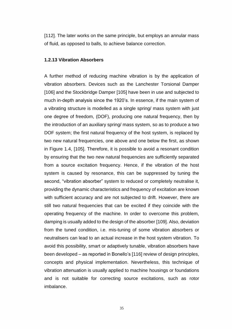
35
[112]. The later works on the same principle, but employs an annular mass
of fluid, as opposed to balls, to achieve balance correction.
1.2.13 Vibration Absorbers
A further method of reducing machine vibration is by the application of
vibration absorbers. Devices such as the Lanchester Torsional Damper
[106] and the Stockbridge Damper [105] have been in use and subjected to
much in-depth analysis since the 1920’s. In essence, if the main system of
a vibrating structure is modelled as a single spring/ mass system with just
one degree of freedom, (DOF), producing one natural frequency, then by
the introduction of an auxiliary spring/ mass system, so as to produce a two
DOF system; the first natural frequency of the host system, is replaced by
two new natural frequencies, one above and one below the first, as shown
in Figure 1.4, [105]. Therefore, it is possible to avoid a resonant condition
by ensuring that the two new natural frequencies are sufficiently separated
from a source excitation frequency. Hence, if the vibration of the host
system is caused by resonance, this can be suppressed by tuning the
second, “vibration absorber” system to reduced or completely neutralise it,
providing the dynamic characteristics and frequency of excitation are known
with sufficient accuracy and are not subjected to drift. However, there are
still two natural frequencies that can be excited if they coincide with the
operating frequency of the machine. In order to overcome this problem,
damping is usually added to the design of the absorber [109]. Also, deviation
from the tuned condition, i.e. mis-tuning of some vibration absorbers or
neutralisers can lead to an actual increase in the host system vibration. To
avoid this possibility, smart or adaptively tunable, vibration absorbers have
been developed – as reported in Bonello’s [116] review of design principles,
concepts and physical implementation. Nevertheless, this technique of
vibration attenuation is usually applied to machine housings or foundations
and is not suitable for correcting source excitations, such as rotor
imbalance.
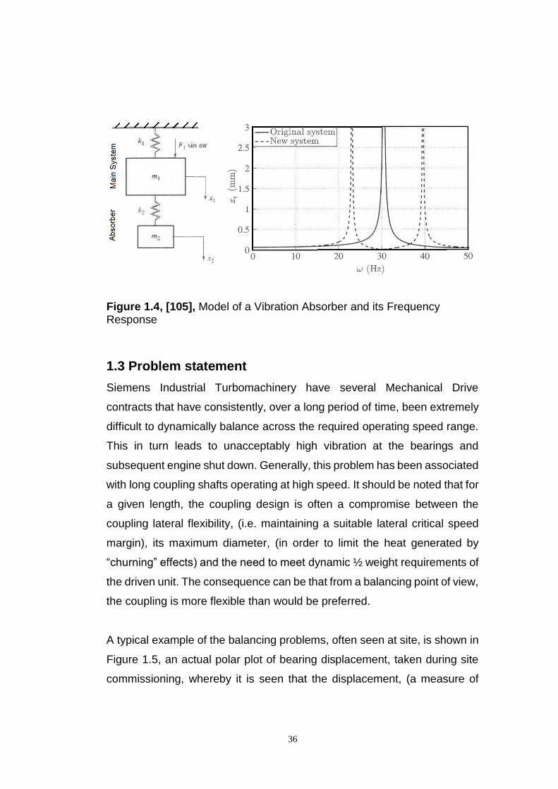
36
Figure 1.4, [105], Model of a Vibration Absorber and its Frequency Response
1.3 Problem statement
Siemens Industrial Turbomachinery have several Mechanical Drive
contracts that have consistently, over a long period of time, been extremely
difficult to dynamically balance across the required operating speed range.
This in turn leads to unacceptably high vibration at the bearings and
subsequent engine shut down. Generally, this problem has been associated
with long coupling shafts operating at high speed. It should be noted that for
a given length, the coupling design is often a compromise between the
coupling lateral flexibility, (i.e. maintaining a suitable lateral critical speed
margin), its maximum diameter, (in order to limit the heat generated by
“churning” effects) and the need to meet dynamic ½ weight requirements of
the driven unit. The consequence can be that from a balancing point of view,
the coupling is more flexible than would be preferred.
A typical example of the balancing problems, often seen at site, is shown in
Figure 1.5, an actual polar plot of bearing displacement, taken during site
commissioning, whereby it is seen that the displacement, (a measure of
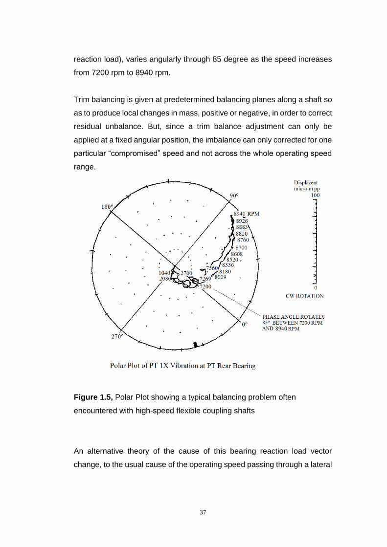
37
reaction load), varies angularly through 85 degree as the speed increases
from 7200 rpm to 8940 rpm.
Trim balancing is given at predetermined balancing planes along a shaft so
as to produce local changes in mass, positive or negative, in order to correct
residual unbalance. But, since a trim balance adjustment can only be
applied at a fixed angular position, the imbalance can only corrected for one
particular “compromised” speed and not across the whole operating speed
range.
Figure 1.5, Polar Plot showing a typical balancing problem often
encountered with high-speed flexible coupling shafts
An alternative theory of the cause of this bearing reaction load vector
change, to the usual cause of the operating speed passing through a lateral
38
critical speed, is demonstrated in Figure 1.6, and its analysis led to a
proposed solution and ultimately to a new balancing methodology.
Figure 1.6, Schematic of PT and Coupling Residual Unbalance Vectors
It was noted that if the coupling shaft, between the engine power turbine
shaft, PT shaft, and the driven unit is sufficiently flexible then, as the
operating speed increases, the magnitude of its unbalance vector can
increase significantly due to its deflection such that it would tend to become
dominant with respect to the neighbouring PT shaft unbalance vector. Then,
the phase angle of the resultant vector, i.e. the bearing reaction load, would
appear to change with speed.
This is shown by the schematic representation in Figure 1.6, where U1 is
the PT residual unbalance vector and U2 is the coupling residual unbalance
vector. Vector U is the resultant of U1 and U2. It can be observed that if U2

39
were to increase in magnitude by a greater amount than that expected due
only to rotational speed, (that is, due to flexing of the coupling shaft), then
the resultant phase angle change with speed can be significant. A worked
example of this is given in chapter 2, section 2.6.
1.4 Aims of this Research
Section 1.2 confirmed that the problems of machine balance and their
subsequent methods of balance reduction stem back more than a century.
However, there remain significant problems with techniques currently being
used. The main techniques for balancing flexible rotors, i.e. Influence
Coefficient and Modal Balancing were introduced in the 1930’s and 1950’s
respectively. Since then improvements in overall balancing methodology
have been largely the result of two distinct changes; 1) a reduction in the
residual eccentricity of the rotating assembly, by advances in machining
capability, (providing tighter tolerances on geometric features, such as
roundness and straightness etc.), plus better control of material properties,
(density, expansion/ contraction, creep etc.) and 2) greater analytical
capability, due to the vast improvement in computing power, thereby
allowing shafts to be analysed to greater depth, into evermore complex
elemental sections. Nevertheless, the basic balancing techniques, although
now producing more accurate results, often in greater detail and in shorter/
less costly time spans, have remained largely unchanged. They still aim to
counter-balance residual eccentricity by making, often multiple, corrections
of trim balance, at various locations along the length of the shaft.
Despite advancements, costly problems remain for industry, as highlighted
in the previous section, thus warranting further investigation. It is the aim of
this research to assess the fundamental deficiencies of current methods of
applying trim balance correction and subsequently to investigate the
application of an improvement, which emanated from this assessment, by
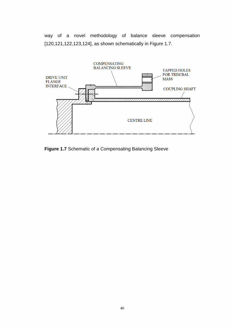
40
way of a novel methodology of balance sleeve compensation
[120,121,122,123,124], as shown schematically in Figure 1.7.
Figure 1.7 Schematic of a Compensating Balancing Sleeve
41
1.5 Main contributions
The following chapters are deemed to offer the most revealing new
insights into improving current methods of balancing high-speed, flexible
shafts.
Chapter 2: this chapter investigated deficiencies of current methods of trim
balance correction and the cause of imbalance vector change, seen at some
problem industrial sites with very flexible couplings. This investigation led to
the invention of a novel method of applying trim balance and further analysis
of a specialised case of uniform eccentricity determined the fundamental
mechanics of balance sleeve compensation.
Chapter 4: this chapter expands the analysis to a generalised case of any
number of concentrated imbalances and determined that conversion to an
equivalent encastre shaft depends on the equalisation of the sum of the
balancing moments to the sum of the encastre fixing moments. This
realisation ultimately leads to simulation being achieved by a single
balancing sleeve at one end only, and subsequently to the ability to
additionally eliminate/nullify the 2nd critical speed.
Chapter 5: this chapter introduces a shear force reaction ratio, RR, which
shows that the proposed methodology has the effect of further reducing the
equivalent level of eccentricity achieved by prior balancing procedures, by
as much as 25x and determines its application to most practical shafting. It
further demonstrates its suitability to higher critical speeds by definition of a
Simulation Ratio, SR, which determines the shaft stiffening effect and the
reaction load reduction benefits to be gained from applying compensation
to shaft ends only.
Chapter 8: presents laboratory test results of a scaled industrial turbine
coupling shaft which supports the analysis determined in the previous

42
chapters and confirms the fundamental requirements of the new balancing
methodology, i.e. that shaft balance is improved by increasing the level of
encastre simulation.
43
Chapter 2
2.1 Causes of Residual Imbalance
Residual imbalance and the centrifugal forces emanating from it during
rotation occurs when the centroid of mass of an elemental section of a shaft
is offset from its axis of rotation. This can occur in a variety of ways, as given
below, but it should be noted that it can never be completely eliminated.
a) Geometric profile errors resulting from imperfect machining. These are
affected by the manufacturing capability to meet the primary machinery
tolerances of roundness, straightness, concentricity, squareness etc. which
can produce oval or bent shafts, or hollow shafts with uneven wall thickness.
b) Material faults, such as non-homogeneous material, with density
variations or inclusions. Also, uneven heat treatment can cause bending of
shafts under differing environmental loading conditions.
c) Interface joint errors are known to be a frequent cause of eccentric
operation or “shafts not running true”. These can result from machining
errors, as above, but also from movement under load with temperature
changes, i.e. spigot and clamping faces, sliding or rocking on high spots.
Also, it is known for spigot clearances to be opened up by centrifugal forces,
thus enabling radial movement to occur. Another, frequent problem seen
with joints is a result of dirt entrapment, preventing proper seating of mating
faces.
d) Gearing problems are often the cause of inconsistent movement of shaft
centres, with load variation or due to machining errors. For example, many
shafts are centralised by forces acting at the point of contact of one or more
meshing gears, which in turn is a function of factors such as: transmitted
torque, lateral loading and mating friction.
44
e) Surface damage can cause displacement of mass, improper seating of
joints or, in exceptional cases, bending of shafts.
The effects of these issues can be minimised by good design and
manufacturing control so that residual imbalance is kept to a minimum.
Nevertheless, perfect balance is never possible and for high-speed shafts,
component and assembly balance procedures are always necessary.
Trim balance corrections are normally made to high-speed shafts in two
stages. First, on low speed balance machines where mass is usually
removed by localised grinding of the outer diameter of a number of
balancing bands - specifically incorporated at intermediate positions along
the shaft length. Secondly, during site commissioning, operating at high
speed, using feedback from the bearing sensors to determine the angular
position and magnitude of added masses, which are usually mounted into
pre-machined, trim balancing tapped holes, at flange interfaces. In both
cases the effect is equivalent to moving the local centroid of mass to
produce a reduced component of eccentricity.
2.2 Trim Balancing Errors and Principle of Improvement
The effectiveness of current methods of trim balancing, with regard to
flexible shafts, is considered as follows. Figure 2.1 shows a typical,
schematic section of a plain flexible shaft, with two elemental sections, one
containing a portion of shaft residual eccentricity, e, and the other
containing a portion of shaft balancing eccentricity eb, produced by the
addition of a trim balance mass, affixed to its outer diameter, (not shown).
For balancing purposes eb is 180º out of phase with e.
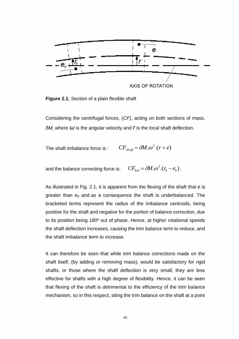
45
Figure 2.1, Section of a plain flexible shaft
Considering the centrifugal forces, (CF), acting on both sections of mass,
δM, where ω is the angular velocity and r is the local shaft deflection.
The shaft imbalance force is : ).(. 2 erMCFshaft
and the balance correcting force is: ).(. 2
bbbal erMCF .
As illustrated in Fig. 2.1, it is apparent from the flexing of the shaft that e is
greater than eb and as a consequence the shaft is underbalanced. The
bracketed terms represent the radius of the imbalance centroids, being
positive for the shaft and negative for the portion of balance correction, due
to its position being 180º out of phase. Hence, at higher rotational speeds
the shaft deflection increases, causing the trim balance term to reduce, and
the shaft imbalance term to increase.
It can therefore be seen that while trim balance corrections made on the
shaft itself, (by adding or removing mass), would be satisfactory for rigid
shafts, or those where the shaft deflection is very small, they are less
effective for shafts with a high degree of flexibility. Hence, it can be seen
that flexing of the shaft is detrimental to the efficiency of the trim balance
mechanism, so in this respect, siting the trim balance on the shaft at a point
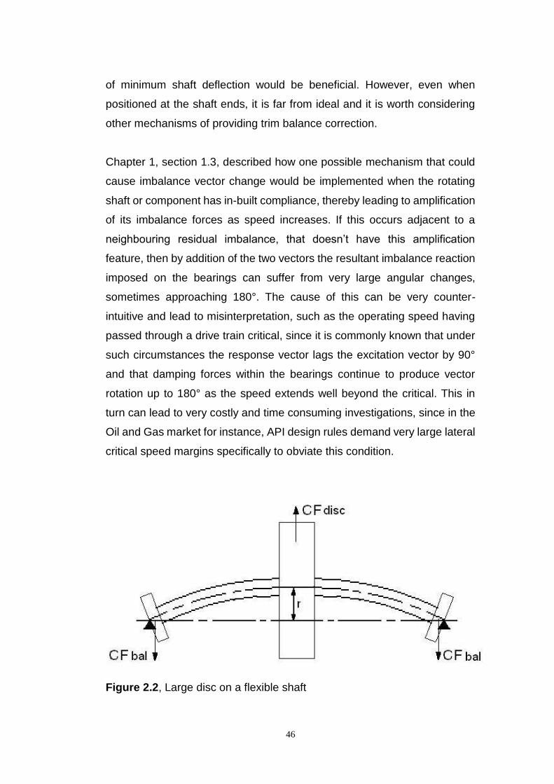
46
of minimum shaft deflection would be beneficial. However, even when
positioned at the shaft ends, it is far from ideal and it is worth considering
other mechanisms of providing trim balance correction.
Chapter 1, section 1.3, described how one possible mechanism that could
cause imbalance vector change would be implemented when the rotating
shaft or component has in-built compliance, thereby leading to amplification
of its imbalance forces as speed increases. If this occurs adjacent to a
neighbouring residual imbalance, that doesn’t have this amplification
feature, then by addition of the two vectors the resultant imbalance reaction
imposed on the bearings can suffer from very large angular changes,
sometimes approaching 180°. The cause of this can be very counter-
intuitive and lead to misinterpretation, such as the operating speed having
passed through a drive train critical, since it is commonly known that under
such circumstances the response vector lags the excitation vector by 90°
and that damping forces within the bearings continue to produce vector
rotation up to 180° as the speed extends well beyond the critical. This in
turn can lead to very costly and time consuming investigations, since in the
Oil and Gas market for instance, API design rules demand very large lateral
critical speed margins specifically to obviate this condition.
Figure 2.2, Large disc on a flexible shaft
47
However, if imbalance amplification is the cause of the problem, then a
possible solution lies in an improved method of trim balance.
To show the impact of shaft flexibility, Figure 2.2 shows a heavy disc,
mounted centrally on a light, flexible shaft, with mounting flanges positioned
at the shaft ends, which are used for trim balancing. It is assumed that the
support bearings, not shown, have very high radial stiffness, but have very
low angular stiffness, such that the shaft can be deemed to be simply
supported. This arrangement is commonly used for analytical purposes and
is known as a Jeffcott rotor. It is chosen here as it simplifies the
mathematics, but still demonstrates a typical drive train problem of obtaining
a suitable balance at both low and high speed. At low speed the shaft is
essentially straight and imbalance, i.e. centrifugal force, CF, acting on the
disc as a result of its eccentricity, disce , is corrected by adding balance
weights at the balance flanges, 180° out of phase, thereby creating
eccentricity at the flanges, bale , so that the vector sum of the CF at the 2
flanges is equal and opposite to the CF at the disc. Hence, the net reaction
load transferred to the bearings is nominally zero.
Hence for balance: discbal CFCF .2 (2.1)
giving, for low speed: discdiscbalbal eMeM .....2 22 (2.2)
and disc
bal
discbal e
M
Me .
.2 (2.3)
where discM = Mass of Disc and balM = Mass of Balance Flange
However, at higher speed the CF acting on the disc increases due to speed,
thereby creating some bending of the shaft, which adds to the disc
eccentricity to further increase disc CF, giving:
48
).(. 2 reMCF discdiscdisc
At the balancing flanges there is negligible shaft deflection so that the only
increase in flange CF is due to the speed increase. Therefore, the balance
criteria given in (2.1) is no longer met and a balancing error occurs that is
proportional to the disc deflection, r,
i.e. the shaft imbalance force, applied to the bearings, = rM disc .. 2 .
Consequently it is not possible to fully balance the shaft for operation at both
low and high speed. The normal solution is to minimise the disc eccentricity
by making balance corrections at the disc, thereby minimising the shaft
deflection, r, but in many drive shafts of more uniform cross section, as in
coupling shafts, for instance, this is not always practical and the result is
generally a balancing compromise over the operating speed range.
To correct the balancing error, it is required that the trim balance weights
should also have a system of compliance to replicate the CF amplification
seen by the disc.
It is noted that this is a very simplified analysis based the balancing criteria
of minimising the reaction loading applied to the bearings, resulting from the
source of the balancing problem given in chapter 1, section 1.3. But, in other
instances, particularly for bladed shaft applications, the balancing objective
can be to reduce shaft deflection/ blade tip clearance, thereby reducing
component wear and improving overall running efficiency.

49
Figure 2.3, Mounting flange with in-built compliance
A simple schematic model of such a system is shown in Figure 2.3, where
a balance ring is flexibly attached to the shaft, allowing radial movement
only, by either a compliant collar or a number of radial springs. The CF
imposed on the balance ring at higher speeds is then resisted by the net
spring compression force and results in a radial deflection, y. Then to
maintain balance, from (2.1), it is required that:
).(.).(..2 22 reMyeM discdiscbalbal
and subtracting (2.2) gives: rMyM discbal ...2 (2.4)
Since no damping exists in this model, the individual CF’s can be equated
directly to their stiffness forces, giving:
50
ySCF balbal . and rSCF shaftdisc .
and substituting in (2.1) gives: rSyS shaftbal ...2
Substituting for r in (2.4) then gives: disc
balshaftbal
M
MSS .
(2.5)
As a practicality check: 2
_
2
_ critshaft
disc
shaft
bal
balcritbal
M
S
M
S
where: critbal_ = critical speed of the balance ring, rad/sec
and critshaft_ = critical speed of the shaft, rad/sec.
Therefore, this very simplified model identifies that by using normal trim
balancing methods, a condition of balance cannot be readily maintained
across a wide operating speed range. But it also suggests a potential
balancing principle, i.e. that by giving the trim balance weights a degree of
compliance an improved shaft balance can be obtained, over a given speed
range, even for a realistic drive train with multiple eccentricities and section
geometry.
It is notable from the above analysis that balS is a constant of practical
magnitude since its critical speed is not less than that of the shaft, and
should therefore allow safe operation of this mechanism, without introducing
lower order critical speeds.
This principle of adding trim balance compliance can clearly be
accomplished by a number of different detail designs, but one method of
providing a spring system, with low hysteresis that maintains the good
design practices required for high speed shafting, i.e. of low half weight,
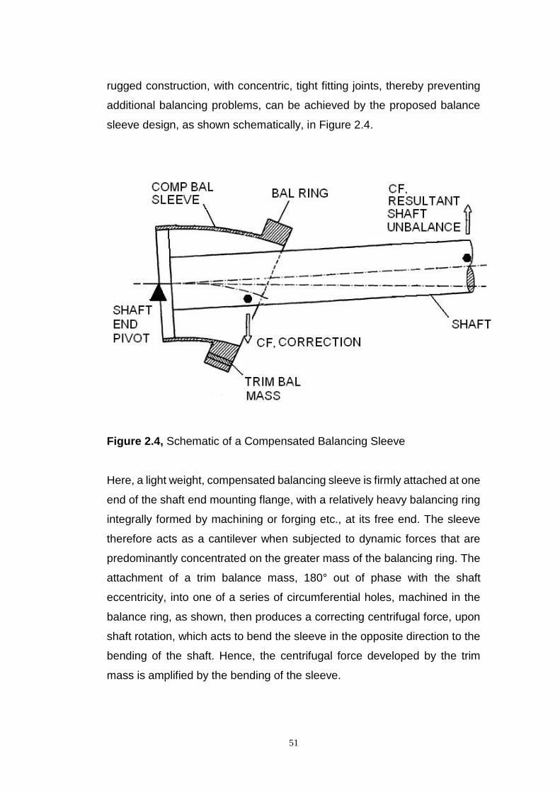
51
rugged construction, with concentric, tight fitting joints, thereby preventing
additional balancing problems, can be achieved by the proposed balance
sleeve design, as shown schematically, in Figure 2.4.
Figure 2.4, Schematic of a Compensated Balancing Sleeve
Here, a light weight, compensated balancing sleeve is firmly attached at one
end of the shaft end mounting flange, with a relatively heavy balancing ring
integrally formed by machining or forging etc., at its free end. The sleeve
therefore acts as a cantilever when subjected to dynamic forces that are
predominantly concentrated on the greater mass of the balancing ring. The
attachment of a trim balance mass, 180° out of phase with the shaft
eccentricity, into one of a series of circumferential holes, machined in the
balance ring, as shown, then produces a correcting centrifugal force, upon
shaft rotation, which acts to bend the sleeve in the opposite direction to the
bending of the shaft. Hence, the centrifugal force developed by the trim
mass is amplified by the bending of the sleeve.
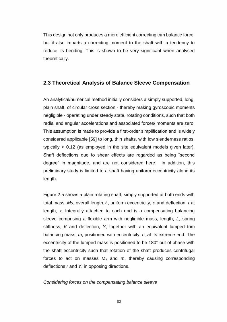
52
This design not only produces a more efficient correcting trim balance force,
but it also imparts a correcting moment to the shaft with a tendency to
reduce its bending. This is shown to be very significant when analysed
theoretically.
2.3 Theoretical Analysis of Balance Sleeve Compensation
An analytical/numerical method initially considers a simply supported, long,
plain shaft, of circular cross section - thereby making gyroscopic moments
negligible - operating under steady state, rotating conditions, such that both
radial and angular accelerations and associated forces/ moments are zero.
This assumption is made to provide a first-order simplification and is widely
considered applicable [59] to long, thin shafts, with low slenderness ratios,
typically < 0.12 (as employed in the site equivalent models given later).
Shaft deflections due to shear effects are regarded as being “second
degree” in magnitude, and are not considered here. In addition, this
preliminary study is limited to a shaft having uniform eccentricity along its
length.
Figure 2.5 shows a plain rotating shaft, simply supported at both ends with
total mass, Ms, overall length, , uniform eccentricity, e and deflection, r at
length, x. Integrally attached to each end is a compensating balancing
sleeve comprising a flexible arm with negligible mass, length, L, spring
stiffness, K and deflection, Y, together with an equivalent lumped trim
balancing mass, m, positioned with eccentricity, c, at its extreme end. The
eccentricity of the lumped mass is positioned to be 180° out of phase with
the shaft eccentricity such that rotation of the shaft produces centrifugal
forces to act on masses Ms and m, thereby causing corresponding
deflections r and Y, in opposing directions.
Considering forces on the compensating balance sleeve
53
ymKY 2 (2.6)
And from inspection of Figure 2.2, for small angles of slope:
0)( xdx
drLcYy
(2.7)
Figure 2.5 Schematic of simply supported rotating shaft with uniform
eccentricity.
giving,
2
0
2 )(
mK
cdx
drLm
Yx
(2.8)
The moment imposed on shaft is: Bdx
drAM
x
0
0
(2.9)
where, 2
22
mK
KLmA
(2.10),
2
2
mK
cLKmB
(2.11)
54
From ‘Bending of Beams’ theory, the dynamic loading imposed on the shaft
is found from (2.9), (noting that 0)( xdx
drA is constant with respect to x),
giving:
Dynamic Loading = 02
0
2
dx
Md
Considering forces on the shaft.
The CF acting on an elemental section δx is: )(2 erxM
CF s
Hence, dynamic loading, at length x is:
)(2 erM
x
CF s
Considering the Combined Assembly
Total Dynamic Loading = 0)(2 erM s
However, from beam theory, the dynamic loading = 4
4
dx
rdEI ,
therefore: 0)(2
4
4
erM
dx
rdEI s
(2.12)
This can be solved by use of Laplace Transforms, where r = Laplace of r, and s is the Laplace Operator:
0)( xo rr
(2.13), 0
1
xdx
drr
(2.14)
0
2
2
2
xdx
rdr
(2.15), 0
3
3
3
xdx
rdr
(2.16)
Hence from (2.12):
es
Mr
MrsrrsrsrsEI ss 22
321
2
0
34 )(
At x = 0: 0r = 0

55
and putting: EI
Mb s
24
(2.17)
then: 31
2
2
444 )( rrssr
s
ebbsr
(2.18)
BM at x = 0: 2
0
2
2
0 EIrdx
rdEIM
x
Therefore from (2.9) and (2.15): EI
BArr
1
2
(2.19)
Substituting in (2.18) gives:
31
21
444 )( rrs
EI
B
EI
Ars
s
ebbsr
letting: EI
BArA
1
1
(2.20), 32 rA
(2.21)
gives: 44
2
44
2
1
44
1
44
4
).( bs
A
bs
sr
bs
sA
bss
ebr
(2.21a)
Each term can be expanded, as given in Appendix A, using Partial Fractions to give:
bs
N
bs
M
bs
Q
bs
sP
s
er
2222
where:
21
22 b
AeP
(2.22), 22
1 221
b
ArQ
(2.23)
321
21
4444 b
Ab
r
b
AeM
(2.24)
321
21
4444 b
Ab
r
b
AeN (2.25)
These terms are now in Standard Laplace form that can be inversed to give:
56
bxbx eNeMbxb
QbxPer ˆˆsincos
(2.26)
where e = Euler’s No.
Applying the following End Conditions:
at x = : r = 0 and BM = 0M and noting, EI
BM
dx
rd
2
2
gives:
bb eNeMbb
QbPe ˆˆsincos0
(2.26a)
bb eNeMbb
QbP
EIb
Moˆˆsincos
2
(2.26b)
(2.26a) – (2.26b) gives: bPEIb
Moeb
b
Qcos
22sin
2
(2.27)
Adding the above: bb eNeM
EIb
Meˆˆ
22 2
0
(2.28)
The exponential terms can be expressed as hyperbolic functions such that:
bHbGeNeM bb sinhcoshˆˆ
(2.29)
where: NMG (2.30) and NMH (2.31)
Substituting in Equation (2.28) gives:
bHbGEIb
Mesinhcosh
22 2
0
(2.32)
and putting (2.27) & (2.29) into (2.26) gives:
bxb
bPEIb
Me
bxPer sinsin
cos22cos
2
0
bxHbxG sinhcosh (2.33)
57
This equation is solvable except for 1r , which a constituent part of the other
unknown parameters; and gives the shaft displacement for given values of
shaft eccentricity, speed and Balancing Sleeve properties, etc.
It is notable that when 00 M the equation reduces to a classical form for
the deflection of a plain rotating shaft with uniform eccentricity [62].
1r is determined by differentiating (2.33) and putting, x = 0 , to give:
bHb
bPEIb
Me
brdx
dr
sin
cos22 2
0
1
(2.34)
Substituting (2.24) and (2.25) in (2.30) and (2.31) gives:
21
22 b
AeG
(2.35) and 321
22 b
Ab
rH
(2.36)
Now, substituting for G in (2.32):
b
bb
AeEIb
Me
Hsinh
cosh2222
21
2
0
(2.37)
and substituting (2.37) in (2.34), gives:
b
bPEIb
Me
brsin
cos22 2
0
1
b
bb
AeEIb
Me
bsinh
cosh)22
(22
21
2
0
Using P from (2.22) and 1A from (2.20) gives:
58
b
bb
EI
BAr
eEIb
Me
brsin
cos2222
2
1
2
0
1
b
bb
EI
BAr
eEIb
Me
bsinh
cosh2222
2
1
2
0
Let: bEIA
2
13 (2.38)
Substituting for Mo from (2.9) gives:
b
bBArAebBArAeb
rsin
cos)(2
)(2
1313
1
b
bBrAebBArAeb
sinh
cosh)(2
)(2
1313
Collating r1 terms and simplifying gives:
bA
bBAebBAeb
rsin
cos22
4
33
1
bA
bBAebBAeb
sinh
cosh22
4
33
(2.39)
Where:
b
bAAAA
b
bAAAAA
sinh
cosh
sin
cos1 3333
4
(2.40)
From beam theory, the vertical shear force within the beam caused by
bending is given by:
3
3
dx
rdEISFv
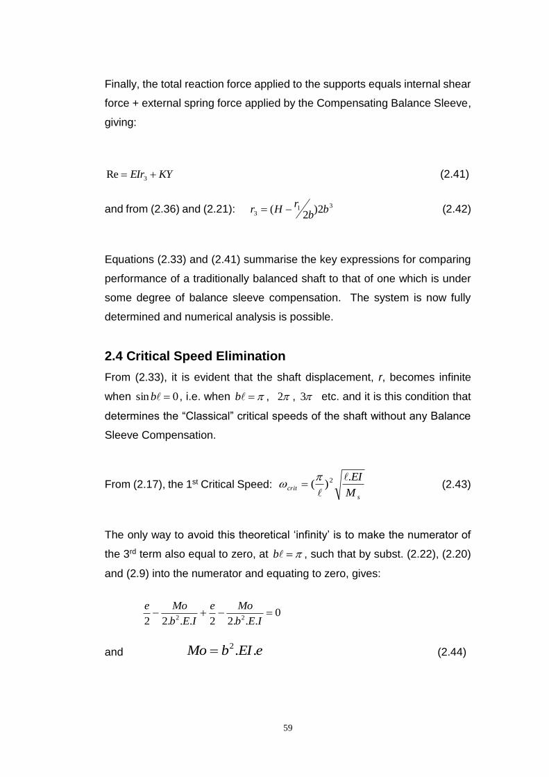
59
Finally, the total reaction force applied to the supports equals internal shear
force + external spring force applied by the Compensating Balance Sleeve,
giving:
KYEIr 3Re (2.41)
and from (2.36) and (2.21): 313 2)
2( b
br
Hr (2.42)
Equations (2.33) and (2.41) summarise the key expressions for comparing
performance of a traditionally balanced shaft to that of one which is under
some degree of balance sleeve compensation. The system is now fully
determined and numerical analysis is possible.
2.4 Critical Speed Elimination
From (2.33), it is evident that the shaft displacement, r, becomes infinite
when 0sin b , i.e. when b , 2 , 3 etc. and it is this condition that
determines the “Classical” critical speeds of the shaft without any Balance
Sleeve Compensation.
From (2.17), the 1st Critical Speed: s
critM
EI.)( 2
(2.43)
The only way to avoid this theoretical ‘infinity’ is to make the numerator of
the 3rd term also equal to zero, at b , such that by subst. (2.22), (2.20)
and (2.9) into the numerator and equating to zero, gives:
0...22...22 22
IEb
Moe
IEb
Moe
and eEIbMo ..2 (2.44)
60
Therefore, by adjusting the Balancing Sleeve parameters so that the
Balancing Moment, eEIbMo ..2 at the speed equivalent to, b ,
makes the 3rd term an indeterminate, 0
0 and hence the effect of the 1st
critical speed is eliminated.
2.5 Analytical Results
The theory described above identifies and solves all the mathematical
‘unknowns’ such that further investigation into balancing compensation can
be carried out by numerical calculations. To this end, a Mathcad program
has been compiled to analyse a simply supported, equivalent model, of the
main drive coupling shaft, used on a sub-15MW, Siemens Gas Turbine,
Compressor Set, using site equivalent parameter values, given in Table 2.1,
below.
* unless otherwise stated
Table 2.1. Parameter Values used in Numerical Example Figures 2.6-2.9 graphically show results from the numerical calculations
derived from equations giving reaction load, (2.41), and midpoint deflection,
Equivalent Site Parameter Values
sM = 38.312 kg = 1.707 m
m = 0.899 kg E = 207.1ˣ10^9 N/m^2
e = 0.00017 m I = 1.468ˣ10^-5 m^4
c = 0.003624 m K = 3.4ˣ10^6 N/m *

61
(2.33), (with x = 2
), for a range of balance compensation conditions. In all
cases the trim balance weights are set to give low speed balance.
Figure 2.6(a). Reaction Load vs. Speed without Balance Sleeve Compensation
Specifically, Figures 2.6(a) and 2.6(b) show shaft end reaction load and
midpoint deflection, plotted against speed, for normal balance conditions,
i.e. without any balance sleeve compensation, modelled as zero sleeve
length and extremely high stiffness. Sleeve length, L = 0 and sleeve
stiffness, K = 3.4×10¹⁶ N/m.

62
Figure 2.6(b). Mid point Deflection vs. Speed without Balance Sleeve Compensation
Figures 2.7(a) and 2.7(b) show reaction load and midpoint deflection, for
very good lateral compensation, providing amplified trim balance correction
of the reaction load only. The midpoint deflection is unaffected since the
sleeve length is still zero – as per the schematic shown in Figure 2.3. Sleeve
length, L = 0 and sleeve stiffness, K = 1.47×10⁶ N/m.
Figure 2.7(a). Reaction Load vs. Speed with Lateral Compensation only
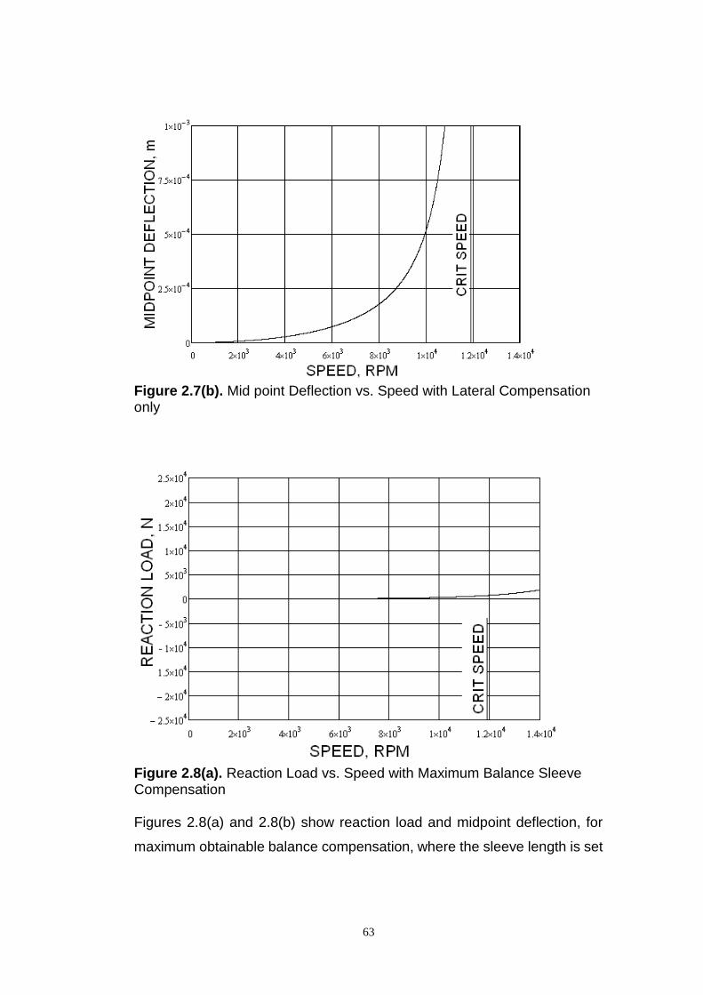
63
Figure 2.7(b). Mid point Deflection vs. Speed with Lateral Compensation only
Figure 2.8(a). Reaction Load vs. Speed with Maximum Balance Sleeve Compensation Figures 2.8(a) and 2.8(b) show reaction load and midpoint deflection, for
maximum obtainable balance compensation, where the sleeve length is set
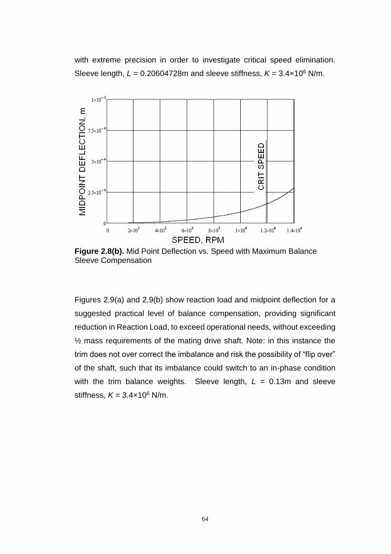
64
with extreme precision in order to investigate critical speed elimination.
Sleeve length, L = 0.20604728m and sleeve stiffness, K = 3.4×10⁶ N/m.
Figure 2.8(b). Mid Point Deflection vs. Speed with Maximum Balance Sleeve Compensation
Figures 2.9(a) and 2.9(b) show reaction load and midpoint deflection for a
suggested practical level of balance compensation, providing significant
reduction in Reaction Load, to exceed operational needs, without exceeding
½ mass requirements of the mating drive shaft. Note: in this instance the
trim does not over correct the imbalance and risk the possibility of “flip over”
of the shaft, such that its imbalance could switch to an in-phase condition
with the trim balance weights. Sleeve length, L = 0.13m and sleeve
stiffness, K = 3.4×10⁶ N/m.
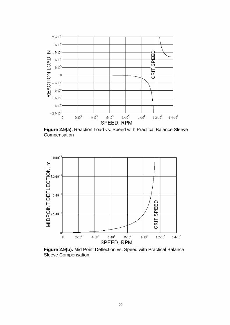
65
Figure 2.9(a). Reaction Load vs. Speed with Practical Balance Sleeve Compensation
Figure 2.9(b). Mid Point Deflection vs. Speed with Practical Balance Sleeve Compensation
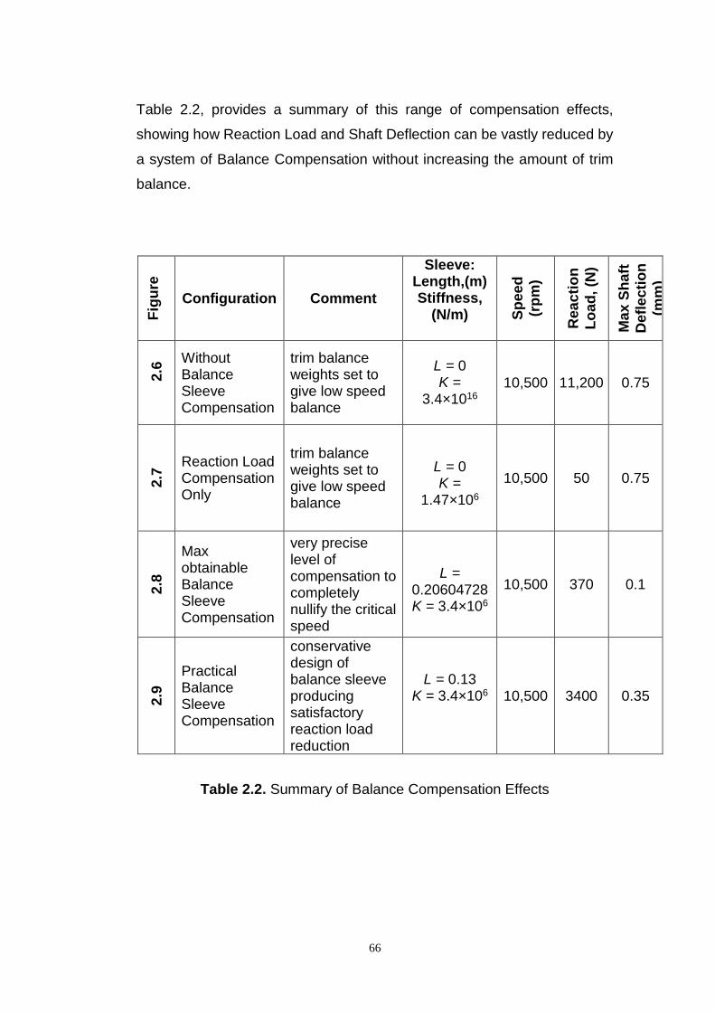
66
Table 2.2, provides a summary of this range of compensation effects,
showing how Reaction Load and Shaft Deflection can be vastly reduced by
a system of Balance Compensation without increasing the amount of trim
balance.
Fig
ure
Configuration Comment
Sleeve: Length,(m) Stiffness,
(N/m) Sp
ee
d
(rp
m)
Rea
cti
on
Lo
ad
, (N
)
Ma
x S
ha
ft
Defl
ec
tio
n
(mm
)
2.6
Without Balance Sleeve Compensation
trim balance weights set to give low speed balance
L = 0 K =
3.4×10¹⁶ 10,500 11,200 0.75
2.7
Reaction Load Compensation Only
trim balance weights set to give low speed balance
L = 0 K =
1.47×10⁶
10,500 50 0.75
2.8
Max obtainable Balance Sleeve Compensation
very precise level of compensation to completely nullify the critical speed
L = 0.20604728 K = 3.4×10⁶
10,500 370 0.1
2.9
Practical Balance Sleeve Compensation
conservative design of balance sleeve producing satisfactory reaction load reduction
L = 0.13 K = 3.4×10⁶ 10,500 3400 0.35
Table 2.2. Summary of Balance Compensation Effects
67
2.6 Site Problem Simulation
Chapter 1, Section 1.3, described a typical balancing problem that is
observed at some Siemens GT sites employing very flexible coupling shafts.
An example characteristic is shown in Figure 1.5 - polar plot of bearing
displacement versus angular displacement, produced a phase angle
change of 85º between operating speeds of 7200 rpm and 8900 rpm. This
means that it is possible to apply a trim balance weight at any particular
angular position, but this only corrects the shaft imbalance at one
corresponding speed; all other speeds remaining unbalanced to a greater
or lesser degree depending on their angular offset from this one speed. It is
therefore extremely difficult to achieve acceptable levels of bearing
displacement, of say less than 60 microns (under normal running
conditions) over the full operating speed range of the turbine.
An alternative theory (to a normal case of operating very close to a critical
speed) for the cause of the vector change is illustrated in Chapter 1, Figure
1.6, suggesting that the root cause of the problem may be due to a very
large increase in the imbalance centrifugal force apportioned to the coupling
shaft deflection.
To corroborate this a theoretical example now assumes that a laterally very
stiff, neighbouring power turbine (PT) shaft, with a residual unbalance vector
of 2000 g.mm, (mass times eccentricity), acted at 150º in opposition to a
coupling shaft, as analysed previously in section 2.5, and detailed in Table
2.1. The equivalent coupling shaft residual unbalance and its trim balance
correction, at shaft ends, are both set to 3257 g.mm, thereby creating
perfect balance at low speed, as shown in Figure 2.10.
Since the PT shaft is very stiff, the bearing reaction load generated by its
imbalance increases with squared speed (unbalance ω2) and is not
subject to the magnification seen by the coupling shaft, due to its flexibility.
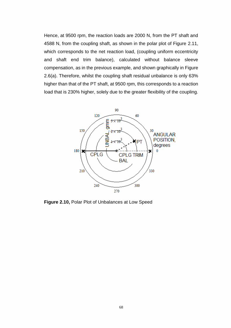
68
Hence, at 9500 rpm, the reaction loads are 2000 N, from the PT shaft and
4588 N, from the coupling shaft, as shown in the polar plot of Figure 2.11,
which corresponds to the net reaction load, (coupling uniform eccentricity
and shaft end trim balance), calculated without balance sleeve
compensation, as in the previous example, and shown graphically in Figure
2.6(a). Therefore, whilst the coupling shaft residual unbalance is only 63%
higher than that of the PT shaft, at 9500 rpm, this corresponds to a reaction
load that is 230% higher, solely due to the greater flexibility of the coupling.
Figure 2.10, Polar Plot of Unbalances at Low Speed

69
Figure 2.11, Polar Plot of Reaction Loads versus Speed
The resultant of the two reaction loads, applied to the bearing can be seen
to rotate from 30º to approximately 160º for speeds increasing from 1500
rpm to 9500 rpm, (shown incrementally in 1000 rpm steps), reaching a
maximum load of 3039 N.
For a typical bearing stiffness of 26.8 106 N/m, the resultant reaction load
corresponds to the bearing displacements shown in Figure 2.12, with the
same vector rotation. It can be seen that the shape and magnitude of this
polar plot closely resembles the equivalent site example, given in Chapter
1, Figure 1.5, thereby providing corroboration with the proposed theory.
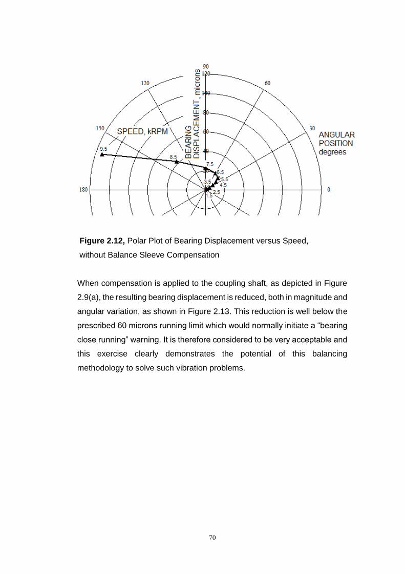
70
Figure 2.12, Polar Plot of Bearing Displacement versus Speed,
without Balance Sleeve Compensation
When compensation is applied to the coupling shaft, as depicted in Figure
2.9(a), the resulting bearing displacement is reduced, both in magnitude and
angular variation, as shown in Figure 2.13. This reduction is well below the
prescribed 60 microns running limit which would normally initiate a “bearing
close running” warning. It is therefore considered to be very acceptable and
this exercise clearly demonstrates the potential of this balancing
methodology to solve such vibration problems.
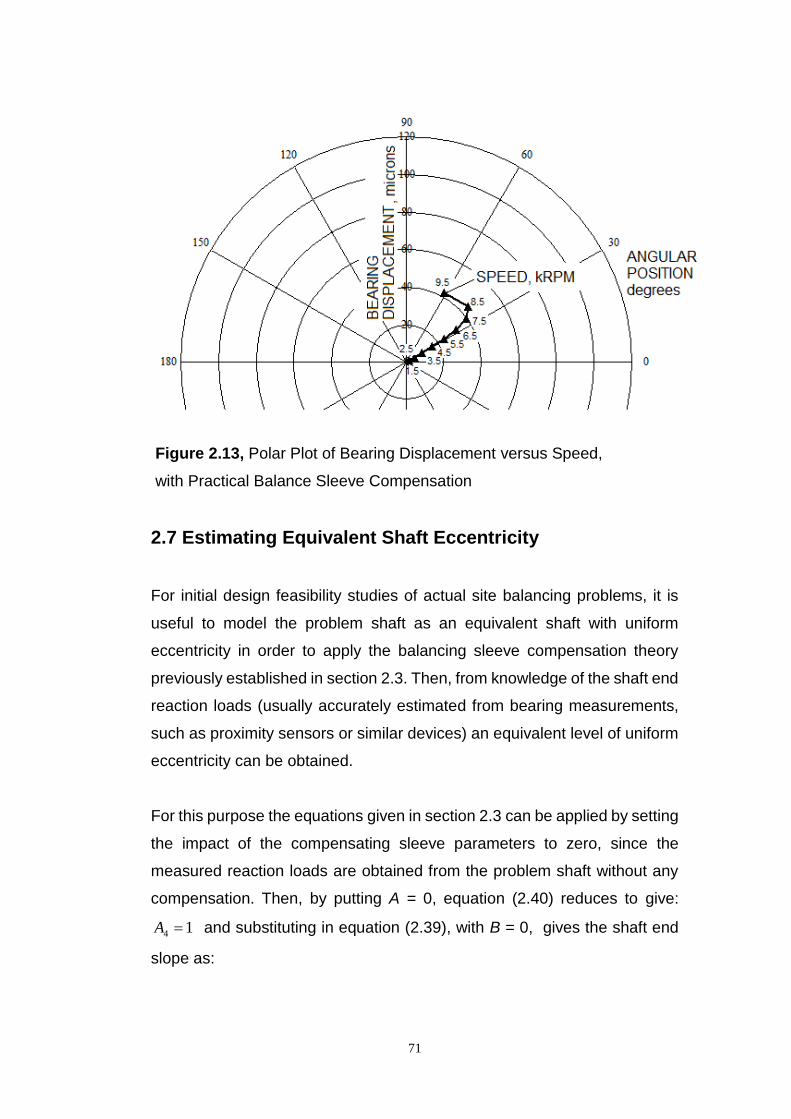
71
Figure 2.13, Polar Plot of Bearing Displacement versus Speed,
with Practical Balance Sleeve Compensation
2.7 Estimating Equivalent Shaft Eccentricity
For initial design feasibility studies of actual site balancing problems, it is
useful to model the problem shaft as an equivalent shaft with uniform
eccentricity in order to apply the balancing sleeve compensation theory
previously established in section 2.3. Then, from knowledge of the shaft end
reaction loads (usually accurately estimated from bearing measurements,
such as proximity sensors or similar devices) an equivalent level of uniform
eccentricity can be obtained.
For this purpose the equations given in section 2.3 can be applied by setting
the impact of the compensating sleeve parameters to zero, since the
measured reaction loads are obtained from the problem shaft without any
compensation. Then, by putting A = 0, equation (2.40) reduces to give:
14 A and substituting in equation (2.39), with B = 0, gives the shaft end
slope as:
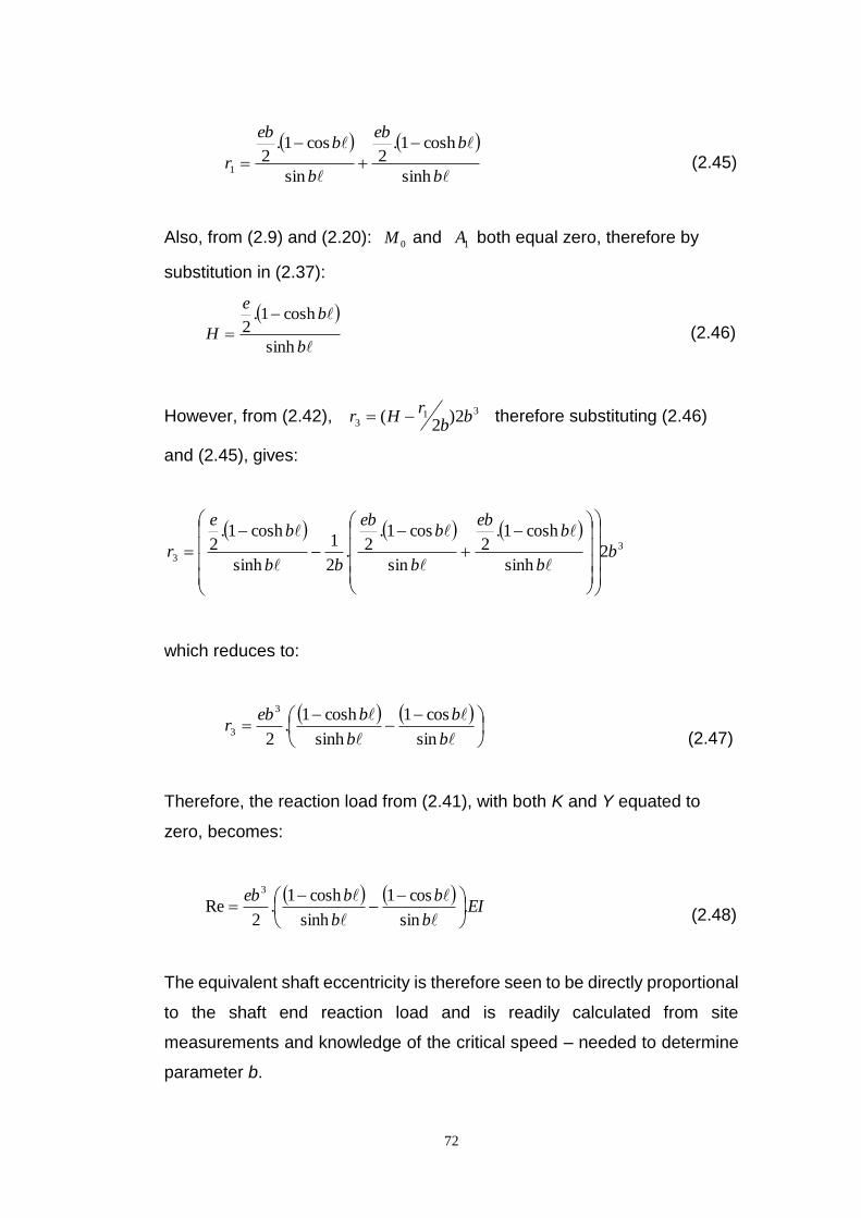
72
b
beb
b
beb
rsinh
cosh1.2
sin
cos1.2
1
(2.45)
Also, from (2.9) and (2.20): 0M and 1A both equal zero, therefore by
substitution in (2.37):
b
be
Hsinh
cosh1.2
(2.46)
However, from (2.42), 313 2)
2( b
br
Hr therefore substituting (2.46)
and (2.45), gives:
3
3 2sinh
cosh1.2
sin
cos1.2.
2
1
sinh
cosh1.2 b
b
beb
b
beb
bb
be
r
which reduces to:
b
b
b
bebr
sin
cos1
sinh
cosh1.
2
3
3 (2.47)
Therefore, the reaction load from (2.41), with both K and Y equated to
zero, becomes:
EIb
b
b
beb.
sin
cos1
sinh
cosh1.
2Re
3
(2.48)
The equivalent shaft eccentricity is therefore seen to be directly proportional
to the shaft end reaction load and is readily calculated from site
measurements and knowledge of the critical speed – needed to determine
parameter b.
73
It is fully expected that by simple modelling of the shaft as having uniform
eccentricity, as illustrated in section 2.6, reasonably accurate conservative
estimates can be made of its eccentricity with sufficient accuracy for
feasibility and initial development design and test purposes, in the
knowledge that, if required, a more detailed finite element analysis (FEA)
could be carried out if necessary.
2.8 Preliminary Conclusions
Consideration of current methods of applying trim balance correction to
rotating shafts show that their effectiveness reduces with increased shaft
flexibility. A new method of adding compliance to the mechanism has been
reported that not only amplifies the magnitude of the balance correcting
forces, but also applies a deflection reducing moment to the shaft. This
method of balance sleeve compensation is shown to have the potential to
vastly reduce the reaction loads applied to the driver and driven unit
bearings. This can be seen from the results summary, Table 2.2, where the
reaction load under normal low speed balance has been reduced from
11,200 N, Figure 2.6(a), to near zero, Figure 2.7(a), at 10,500 rpm. This
latter condition represents lateral balance compensation only in accordance
with the schematic shown in Figure 2.3, where the trim balance centrifugal
force has been amplified, but only acts upon the mounting flange without
applying a correcting moment to the shaft. Hence, the shaft deflection has
not been reduced.
A much improved method of providing trim balance compliance is shown
in Figure 2.4, with the added benefit of applying the balancing moment,
0M , which also reduces the shaft deflection as shown in Table 2.2,
Figures 2.8(b) and 2.9(b), giving mid-point shaft deflection reduction from
0.75 mm to 0.1 mm and 0.35 mm, respectively, at 10,500 rpm.

74
The case shown in Figure 2.8, attempts to maximise the balance
compensation and also investigate possible critical speed elimination, as
mathematically shown section 2.4 (hence the 8 digit sleeve length, L). The
results are therefore very positive with vast reductions in both reaction load
and mid-point deflection being evident. Nevertheless, it is notable that this
is only a theoretical possibility and a more practical condition is shown in
Figure 2.9. This latter condition is considered good design compromise, as
it still provides significant reduction in reaction load, to exceed operational
needs, without excessive balancing sleeve length and/ or deflection.
This is also confirmed by the treatment in section 2.6, of the typical
balancing problems observed at some problematic GT sites employing
relatively flexible couplings, and highlighted in chapter 1. An alternative
proposal for the vibration source, that the angular change of the bearing
imbalance vector was a result of the coupling unbalance being amplified by
its deflection, has also been corroborated. Further, the example has shown
that application of balancing sleeve compensation can reduce the bearing
deflection to acceptable limits, by reducing the coupling reaction load and
also, as a consequence, reduce the angular change of the imbalance
vector.
Section 2.7 showed that the uniform eccentricity of an equivalent shaft, is
directly proportional to shaft end reaction load and therefore readily
estimated, hence this analytical model can usefully be employed in design
and feasibility investigations.
Further investigation of critical speed and the reduction of its impact using
an analysis of Balance Sleeve Compensation, is now given in chapter 3.
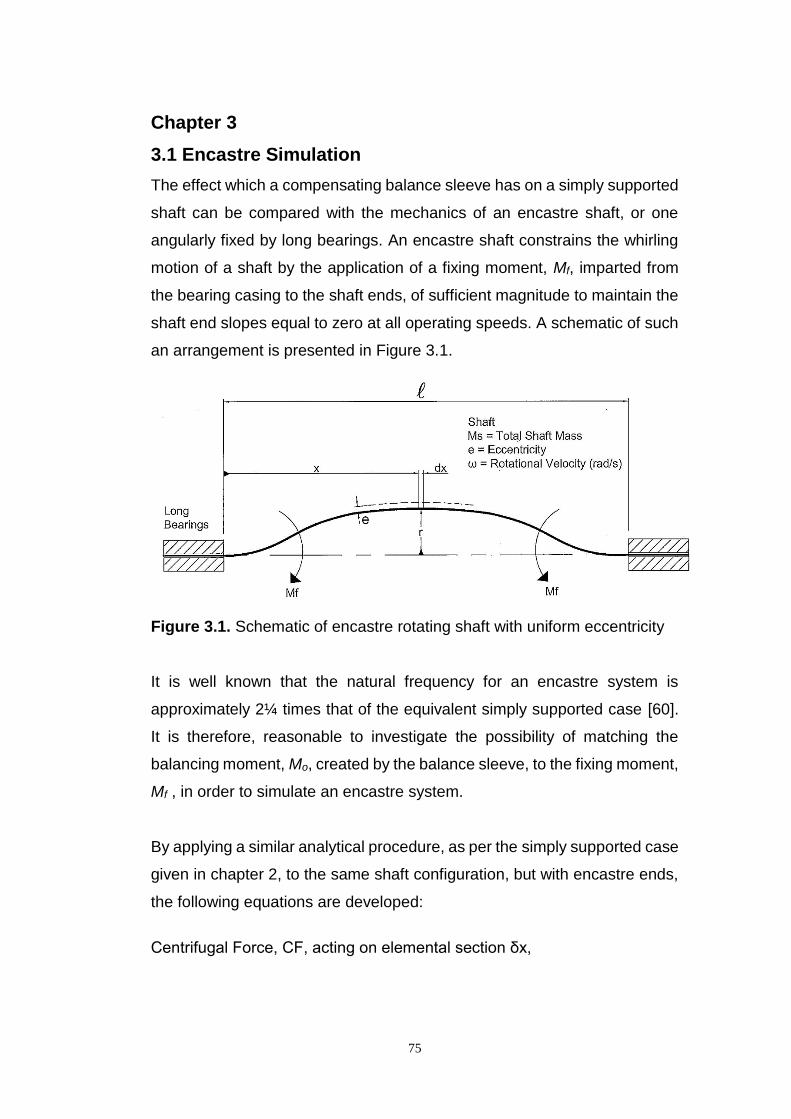
75
Chapter 3
3.1 Encastre Simulation
The effect which a compensating balance sleeve has on a simply supported
shaft can be compared with the mechanics of an encastre shaft, or one
angularly fixed by long bearings. An encastre shaft constrains the whirling
motion of a shaft by the application of a fixing moment, Mf, imparted from
the bearing casing to the shaft ends, of sufficient magnitude to maintain the
shaft end slopes equal to zero at all operating speeds. A schematic of such
an arrangement is presented in Figure 3.1.
Figure 3.1. Schematic of encastre rotating shaft with uniform eccentricity
It is well known that the natural frequency for an encastre system is
approximately 2¼ times that of the equivalent simply supported case [60].
It is therefore, reasonable to investigate the possibility of matching the
balancing moment, Mo, created by the balance sleeve, to the fixing moment,
Mf , in order to simulate an encastre system.
By applying a similar analytical procedure, as per the simply supported case
given in chapter 2, to the same shaft configuration, but with encastre ends,
the following equations are developed:
Centrifugal Force, CF, acting on elemental section δx,
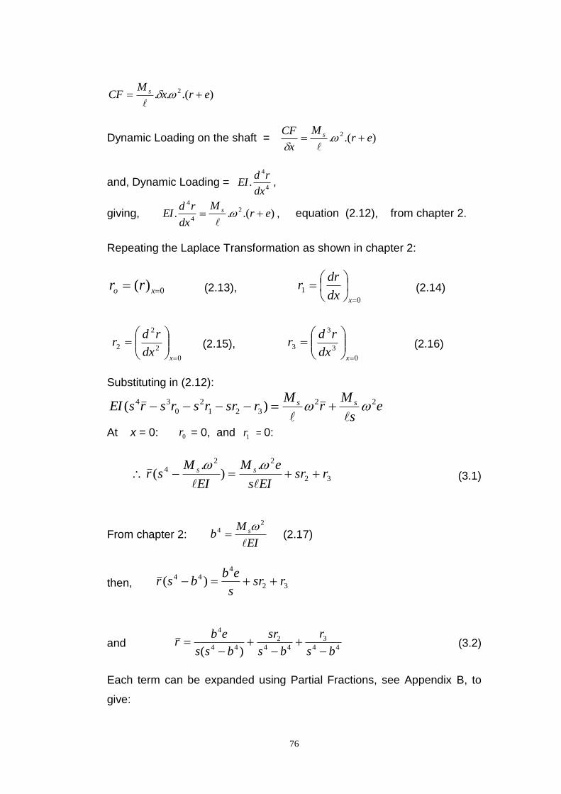
76
).(.. 2 erxM
CF s
Dynamic Loading on the shaft = ).(. 2 erM
x
CF s
and, Dynamic Loading = 4
4
.dx
rdEI ,
giving, ).(.. 2
4
4
erM
dx
rdEI s
, equation (2.12), from chapter 2.
Repeating the Laplace Transformation as shown in chapter 2:
0)( xo rr
(2.13), 0
1
xdx
drr
(2.14)
0
2
2
2
xdx
rdr
(2.15), 0
3
3
3
xdx
rdr
(2.16)
Substituting in (2.12):
es
Mr
MrsrrsrsrsEI ss 22
321
2
0
34 )(
At x = 0: 0r = 0, and 1r = 0:
32
22
4 .)
.( rsr
EIs
eM
EI
Msr ss
(3.1)
From chapter 2: EI
Mb s
24
(2.17)
then, 32
444 )( rsr
s
ebbsr
and 44
3
44
2
44
4
)( bs
r
bs
sr
bss
ebr
(3.2)
Each term can be expanded using Partial Fractions, see Appendix B, to
give:

77
bs
N
bs
M
bs
Q
bs
Ps
s
er eeee
2222
. (3.3)
where:
22
22 b
rePe ,
23
2b
rQe
, 3
32
2
444 b
r
b
reM e
33
22
444 b
r
b
reNe (3.3a)
These terms are now in Standard Laplace forms which can be inverted to give:
bx
e
bx
ee
e eNeMbxb
QbxPer ˆ.ˆ.sincos ,
where e = exponential value, e.
However, the exponential terms can be expressed as Hyperbolic Functions,
as given Appendix C, where x represents any angle, i.e. in this case, x = bx
to give:
bxHbxGbxJbxPer eee sinhcoshsincos (3.4)
where b
QJ e , eee NMG , eee MNH (3.4a)
but r = 0 at x = 0, ee GPe 0 and ee PeG (3.5)
Differentiating (3.4), xbHxbGbxbJbxbPdx
dreee coshsinhcos.sin
And 0dx
dr at x = 0, ebHbJ 0 and JH e (3.6)
Substituting (3.5) & (3.6) in (3.4) gives:
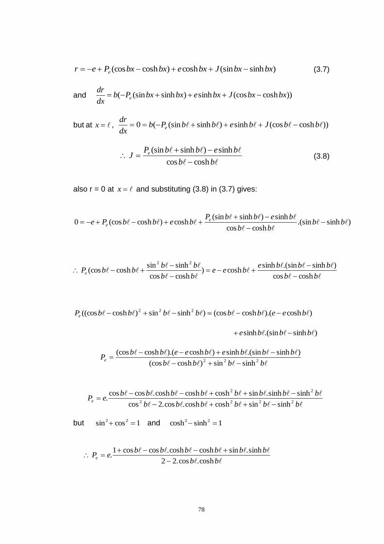
78
)sinh(sincosh)cosh(cos bxbxJbxebxbxPer e (3.7)
and ))cosh(cossinh)sinh(sin( bxbxJbxebxbxPbdx
dre
but at x , ))cosh(cossinh)sinh(sin(0 bbJbebbPbdx
dre
bb
bebbPJ e
coshcos
sinh)sinh(sin
(3.8)
also r = 0 at x and substituting (3.8) in (3.7) gives:
)sinh.(sincoshcos
sinh)sinh(sincosh)cosh(cos0
bb
bb
bebbPbebbPe e
e
bb
bbbebee
bb
bbbbPe
coshcos
)sinh.(sinsinhcosh)
coshcos
sinhsincosh(cos
22
)cosh).(cosh(cos)sinhsin)cosh((cos 222 beebbbbbbPe
)sinh.(sinsinh bbbe
bbbb
bbbebeebbPe 222 sinhsin)cosh(cos
)sinh.(sinsinh)cosh).(cosh(cos
bbbbbb
bbbbbbbbePe 2222
22
sinhsincoshcosh.cos.2cos
sinhsinh.sincoshcoshcosh.coscos.
but 1cossin 22 and 1sinhcosh 22
bb
bbbbbbePe
cosh.cos.22
sinh.sincoshcosh.coscos1.
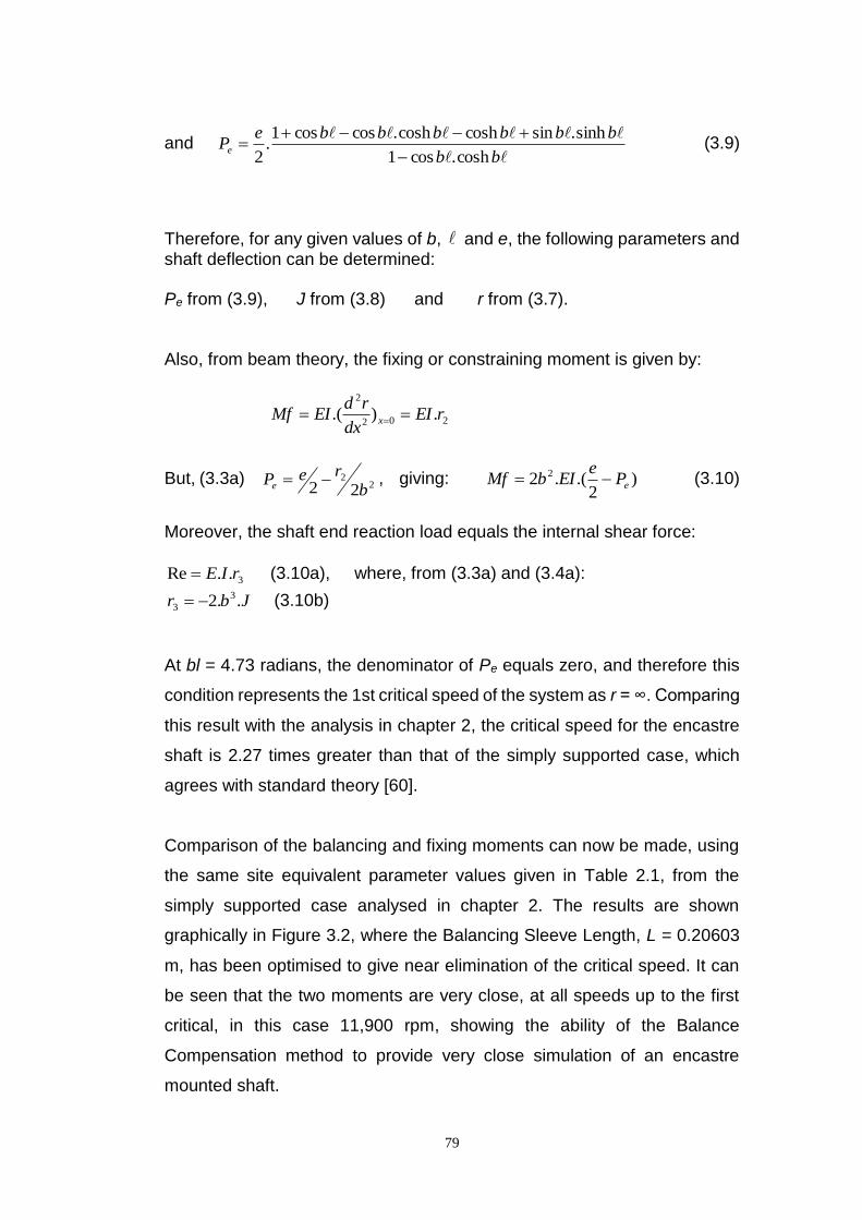
79
and
bb
bbbbbbePe
cosh.cos1
sinh.sincoshcosh.coscos1.
2
(3.9)
Therefore, for any given values of b, and e, the following parameters and shaft deflection can be determined: Pe from (3.9), J from (3.8) and r from (3.7). Also, from beam theory, the fixing or constraining moment is given by:
202
2
.).( rEIdx
rdEIMf x
But, (3.3a) 22
22 b
rePe , giving: )2
.(.2 2
ePe
EIbMf (3.10)
Moreover, the shaft end reaction load equals the internal shear force:
3..Re rIE (3.10a), where, from (3.3a) and (3.4a):
Jbr ..2 3
3 (3.10b)
At bl = 4.73 radians, the denominator of Pe equals zero, and therefore this
condition represents the 1st critical speed of the system as r = ∞. Comparing
this result with the analysis in chapter 2, the critical speed for the encastre
shaft is 2.27 times greater than that of the simply supported case, which
agrees with standard theory [60].
Comparison of the balancing and fixing moments can now be made, using
the same site equivalent parameter values given in Table 2.1, from the
simply supported case analysed in chapter 2. The results are shown
graphically in Figure 3.2, where the Balancing Sleeve Length, L = 0.20603
m, has been optimised to give near elimination of the critical speed. It can
be seen that the two moments are very close, at all speeds up to the first
critical, in this case 11,900 rpm, showing the ability of the Balance
Compensation method to provide very close simulation of an encastre
mounted shaft.

80
Figure 3.2. Fixing and balancing moment vs speed, with maximum
compensation
It is also interesting to note that at b , i.e. the Classical Critical Speed
of the simply supported system, Pe = 0 and the encastre fixing moment
becomes,
eEIbMf ..2 (3.11)
which is identical to equation (2.44), chapter 2, the balancing moment
required for elimination of the simply supported, 1st critical speed; therefore,
at this speed, MfMo , and complete encastre simulation occurs at the
intersection point between the two curves shown in Figure 3.2.

81
3.2 Compensated Critical Speeds
To further investigate encastre simulation and the resulting elimination of
the simply supported critical speed, it is necessary to extend the analysis
given in chapter 2.
For a Simply Supported Shaft System with Balancing Sleeve
Compensation, equation (2.40) states:
b
bAAAA
b
bAAAAA
sinh
cosh
sin
cos1 3333
4
and at the Classical Critical speed, equivalent to, b , this becomes:
sinh
cosh...
0
..1 3333
4
AAAAAAAAA
The 1st and 3rd terms can be ignored as negligible compared to 2nd term:
0
..2 3
4
AAA
Also from (2.39), the slope of the shaft at x=0, is given by
bA
bBAebBAeb
rsin
cos22
4
33
1
bA
bBAebBAeb
sinh
cosh22
4
33
which reduces to, 0
0.0
..2
)1).(.2
.(.2
.
3
33
1
AA
BAbeBAbe
r and:
A
BA
be
AA
BAber
3
3
3
1
.2
.
..2
..2.
82
Hence: MoA
beBrA
3
1.2
..
Making substitutions bEI
A2
13 , (2.38) and
EI
Mb s
24
(2.17)
gives eEIbMo ..2 and eEIMo ..
2
(3.12)
This has far reaching implications since it shows that Mo is independent of
the Balance Sleeve parameters: mass, eccentricity, length and stiffness and
gives a constant value for a given shaft when running at its standard,
classical critical speed.
Also, since this equation is identical to (2.44), for b , it means that the
classical critical is always eliminated, regardless of the characteristics of
Mo.
This is best illustrated graphically, using the parameter values given in Table
2.1, which shows that ALL levels of positive Balancing Sleeve Moment, Mo,
plus the Fixing Moment, Mf, coincide at a point of convergence, given by
equation (3.12), at the speed defined by equation (2.43). See Figure 3.3,
below – where 3 characteristics of Mo were plotted, using 3 different
Compensating Sleeve Lengths, L.

83
Figure 3.3. Close-up of point of convergence.
It is noted that the only time the Point of Convergence is avoided is when
Mo = 0 and then the critical speed reverts to its Classical value.
From the above it is apparent that b , 2 , 3 only defines the critical
speeds for simply supported shafts without any externally applied moments,
i.e. when Mo equals zero. But, for all other arrangements the 1st critical
speed can be seen to have moved away from the standard theoretical
speed by a few hundred rpm. This is evident from Figure 3.3, which shows
Mo tending to infinity, at speeds away from the Point of Convergence, and
this is as a consequence of the slope 1r becoming infinite.
Therefore, this condition can be used to determine the new Compensated
Critical Speed.
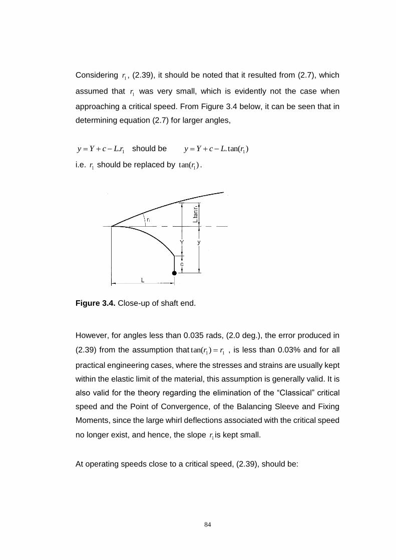
84
Considering 1r , (2.39), it should be noted that it resulted from (2.7), which
assumed that 1r was very small, which is evidently not the case when
approaching a critical speed. From Figure 3.4 below, it can be seen that in
determining equation (2.7) for larger angles,
1.rLcYy should be )tan(. 1rLcYy
i.e. 1r should be replaced by )tan( 1r .
Figure 3.4. Close-up of shaft end.
However, for angles less than 0.035 rads, (2.0 deg.), the error produced in
(2.39) from the assumption that 11)tan( rr , is less than 0.03% and for all
practical engineering cases, where the stresses and strains are usually kept
within the elastic limit of the material, this assumption is generally valid. It is
also valid for the theory regarding the elimination of the “Classical” critical
speed and the Point of Convergence, of the Balancing Sleeve and Fixing
Moments, since the large whirl deflections associated with the critical speed
no longer exist, and hence, the slope 1r is kept small.
At operating speeds close to a critical speed, (2.39), should be:

85
bA
bBAebBAeb
rsin
cos22)tan(
4
33
1
bA
bBAebBAeb
sinh
cosh22
4
33
(3.13)
such that at a critical speed the slope becomes vertical and )tan( 1r equals
infinity and it can be seen that this will occur when 04 A .
From chapter 2:
b
bAAAA
b
bAAAAA
sinh
cosh
sin
cos1 3333
4
, (2.40)
and by substituting the following trigonometric relationships:
x
xx
sin
cos1
2tan
,
2sinh
2coshcosh 22 xx
x ,
2cosh.
2sinh.2sinh
xxx , xx 22 sinhcosh1 ,
gives:
2cosh.
2sinh.2
)2
sinh2
cosh1(
2tan..1
22
34
bb
bb
bAAA
2cosh.
2sinh.2
2sinh.2
2tan..1
2
34
bb
b
bAAA . Substituting
bEIA
2
13 , (2.38)
gives: )2
tanh2
.(tan...2
14
bb
IEb
AA (3.14)
Since at the critical speed 04 A and it is known that this occurs at a speed
close to the equivalent of b , whereby the tanh term tends to 1, the
compensated critical speed can be defined by the condition where:
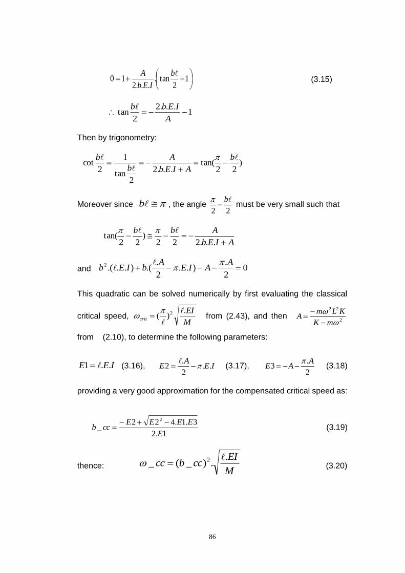
86
1
2tan.
...210
b
IEb
A (3.15)
1...2
2tan
A
IEbb
Then by trigonometry:
)22
tan(...2
2tan
1
2cot
b
AIEb
A
b
b
Moreover since b , the angle 22
b
must be very small such that
AIEb
Abb
...222)
22tan(
and 02
.)..
2
..()...(2
AAIE
AbIEb
This quadratic can be solved numerically by first evaluating the classical
critical speed, M
EIcrit
.)( 2
from (2.43), and then
2
22
mK
KLmA
from (2.10), to determine the following parameters:
IEE ..1 (3.16), IEA
E ..2
.2
(3.17),
2
.3
AAE
(3.18)
providing a very good approximation for the compensated critical speed as:
1.2
3.1.422_
2
E
EEEEccb
(3.19)
thence: M
EIccbcc
..)_(_ 2
(3.20)
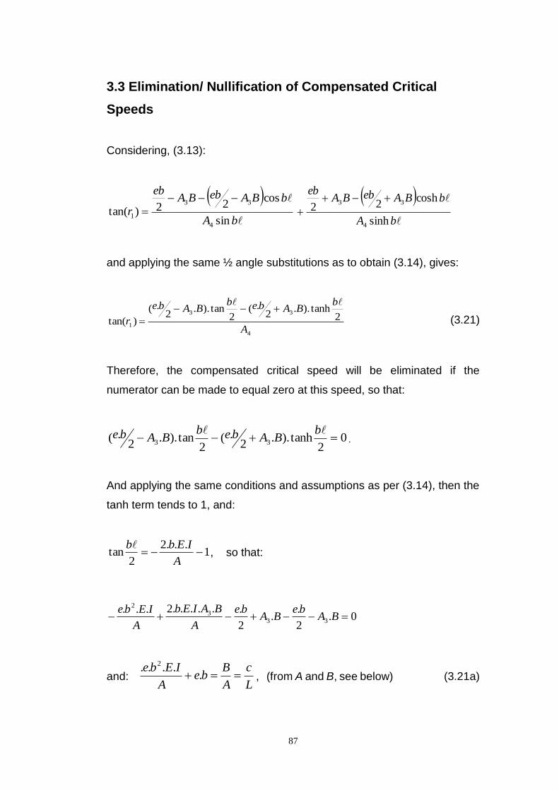
87
3.3 Elimination/ Nullification of Compensated Critical
Speeds
Considering, (3.13):
bA
bBAebBAeb
rsin
cos22)tan(
4
33
1
bA
bBAebBAeb
sinh
cosh22
4
33
and applying the same ½ angle substitutions as to obtain (3.14), gives:
4
33
1
2tanh)..
2.(
2tan)..
2.(
)tan(A
bBAbeb
BAbe
r
(3.21)
Therefore, the compensated critical speed will be eliminated if the
numerator can be made to equal zero at this speed, so that:
02
tanh)..2
.(2
tan)..2
.( 33 b
BAbebBAbe .
And applying the same conditions and assumptions as per (3.14), then the
tanh term tends to 1, and:
1...2
2tan
A
IEbb, so that:
0.2
..
2
......2...33
3
2
BAbe
BAbe
A
BAIEb
A
IEbe
and: L
c
A
Bbe
A
IEbe .
.... 2
, (from A and B, see below) (3.21a)
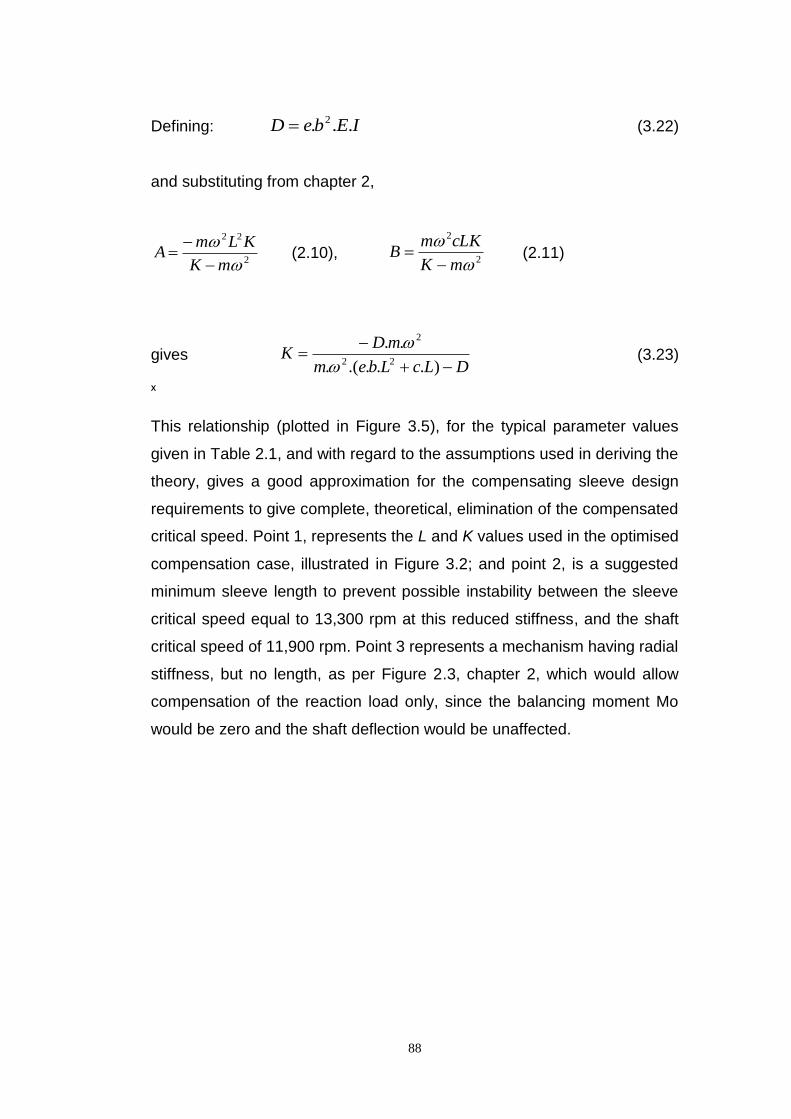
88
Defining: IEbeD ... 2 (3.22) and substituting from chapter 2,
2
22
mK
KLmA
(2.10),
2
2
mK
cLKmB
(2.11)
gives DLcLbem
mDK
)....(.
..22
2
(3.23)
ˣ This relationship (plotted in Figure 3.5), for the typical parameter values
given in Table 2.1, and with regard to the assumptions used in deriving the
theory, gives a good approximation for the compensating sleeve design
requirements to give complete, theoretical, elimination of the compensated
critical speed. Point 1, represents the L and K values used in the optimised
compensation case, illustrated in Figure 3.2; and point 2, is a suggested
minimum sleeve length to prevent possible instability between the sleeve
critical speed equal to 13,300 rpm at this reduced stiffness, and the shaft
critical speed of 11,900 rpm. Point 3 represents a mechanism having radial
stiffness, but no length, as per Figure 2.3, chapter 2, which would allow
compensation of the reaction load only, since the balancing moment Mo
would be zero and the shaft deflection would be unaffected.
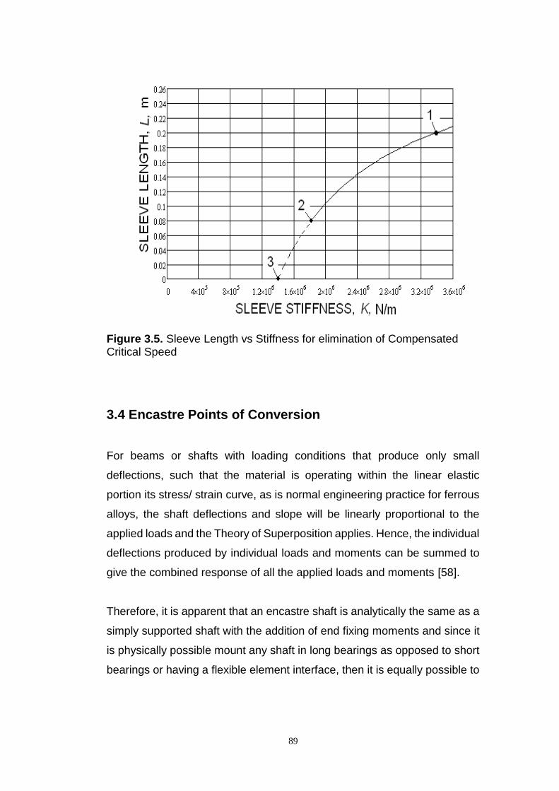
89
Figure 3.5. Sleeve Length vs Stiffness for elimination of Compensated Critical Speed
3.4 Encastre Points of Conversion
For beams or shafts with loading conditions that produce only small
deflections, such that the material is operating within the linear elastic
portion its stress/ strain curve, as is normal engineering practice for ferrous
alloys, the shaft deflections and slope will be linearly proportional to the
applied loads and the Theory of Superposition applies. Hence, the individual
deflections produced by individual loads and moments can be summed to
give the combined response of all the applied loads and moments [58].
Therefore, it is apparent that an encastre shaft is analytically the same as a
simply supported shaft with the addition of end fixing moments and since it
is physically possible mount any shaft in long bearings as opposed to short
bearings or having a flexible element interface, then it is equally possible to

90
convert any shaft, of any geometric or loading variation, to an encastre form,
by equating the balancing moment, Mo, to the fixing moment, Mf.
This then is the rational objective of critical speed elimination, i.e. to adjust
the Balancing Sleeve Moment, Mo, so that it equals the encastre Fixing
Moment, Mf. Unfortunately, it is not possible to maintain this condition
throughout the whole of the operating speed range, but it is advantageous
if it occurs at a speed as close as possible to the Compensated Critical
Speed, so that near elimination results.
This adjustment process is illustrated in Figure 3.6 and 3.7 below.
Figure 3.6, shows a close up example of the both moments near the critical
speeds, and it can be seen that there are 3 points of intersection, where Mo
= Mf, and conversion occurs.
Point 1 occurs at the Compensated Critical Speed, where Mo
instantaneously passes from minus infinity to plus infinity. This is only a
theoretical possibility and consequently it is not a practical point of
conversion. Note, this speed varies only slightly with Compensating Sleeve
Length, L.
Point 2 occurs at the Classical Critical Speed, which, as defined earlier, is
fixed speed and doesn’t vary with length L.
Point 3 is the natural intersection of the 2 curves that would occur without
the interruption of the critical speed points and is highly dependent on the
magnitude of L. Hence, it is more adjustable and L can be used as a design
variable – note, it moves to a lower speed with increasing length, L and vice
versa.
Figure 3.7, shows how easily point 3 can be adjusted and the effect of a
small increase in length L, from 0.20m to 0.20603m, where it can be seen
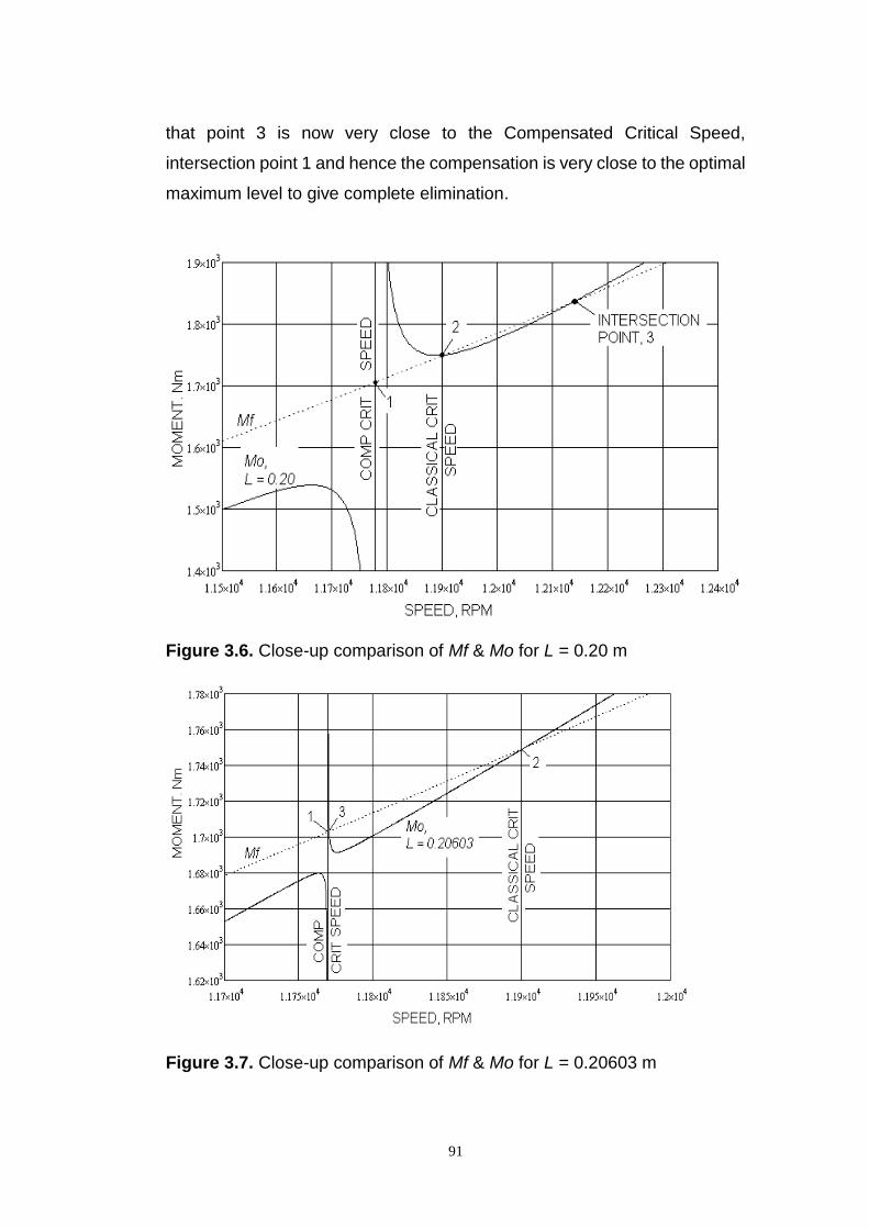
91
that point 3 is now very close to the Compensated Critical Speed,
intersection point 1 and hence the compensation is very close to the optimal
maximum level to give complete elimination.
Figure 3.6. Close-up comparison of Mf & Mo for L = 0.20 m
Figure 3.7. Close-up comparison of Mf & Mo for L = 0.20603 m
92
Exact coincidence would result in complete elimination, which although
theoretically possible, is not practical due to the infinite sensitivity of the
transient. It can also be noted, that the closer points 1 and 3 become, then
the sharper the critical speed spike becomes, thereby minimizing the
magnifying effect of the critical speed and allowing safe operation much
closer to its critical speed than would otherwise be possible.
At the practical points of intersection, 2 and 3, where Mo = Mf, numerical
analysis can be used to show that the shaft deflections and internal shear
reaction forces are identical, thereby confirming that the points of
intersection are indeed Points of Conversion where the simply supported
shaft fully replicates the encastre system, albeit only for the speeds where
the intersection occurs.
3.5 Practical Possibility of Critical Speed Elimination
Furthering the analytical investigation carried out in chapter 2, with the site
equivalent parameter values, given in Table 2.1, the maximum obtainable
balance compensation condition, Figure 2.6, chapter 2, is investigated.
Figure 3.8, below shows a close up of this condition, in which the reaction
load has been calculated and plotted against rotational speed in very fine
steps of only 0.1 rpm. However, it can be seen that the critical speed has
still not been completely eliminated as a spike still occurs between 11,769.3
rpm and 11,769.5 rpm, which would go to infinity if the calculated speed
could be made exactly equal to the compensated critical speed.
Nevertheless, it can be seen that the act of balance sleeve compensation
makes the critical speed spike much sharper until at full compensation it
would be possible to theoretically operate to within 1 rpm of the actual critical
speed, i.e. it is reasonable to conclude that the critical speed has been
completely NULLIFIED. Note, actual elimination of the critical speed would
be practically impossible since the parameter values etc. undoubtedly
contain irrational numbers such as . However, while such proximity would
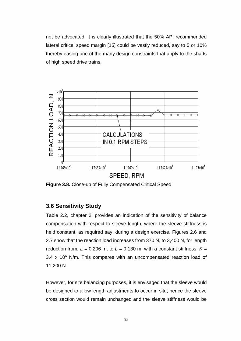
93
not be advocated, it is clearly illustrated that the 50% API recommended
lateral critical speed margin [15] could be vastly reduced, say to 5 or 10%
thereby easing one of the many design constraints that apply to the shafts
of high speed drive trains.
Figure 3.8. Close-up of Fully Compensated Critical Speed
3.6 Sensitivity Study
Table 2.2, chapter 2, provides an indication of the sensitivity of balance
compensation with respect to sleeve length, where the sleeve stiffness is
held constant, as required say, during a design exercise. Figures 2.6 and
2.7 show that the reaction load increases from 370 N, to 3,400 N, for length
reduction from, L = 0.206 m, to L = 0.130 m, with a constant stiffness, K =
3.4 x 10⁶ N/m. This compares with an uncompensated reaction load of
11,200 N.
However, for site balancing purposes, it is envisaged that the sleeve would
be designed to allow length adjustments to occur in situ, hence the sleeve
cross section would remain unchanged and the sleeve stiffness would be
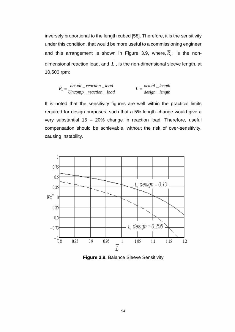
94
inversely proportional to the length cubed [58]. Therefore, it is the sensitivity
under this condition, that would be more useful to a commissioning engineer
and this arrangement is shown in Figure 3.9, where, eR , is the non-
dimensional reaction load, and L , is the non-dimensional sleeve length, at
10,500 rpm:
loadreactionUncomp
loadreactionactualRe
__
__
lengthdesign
lengthactualL
_
_
It is noted that the sensitivity figures are well within the practical limits
required for design purposes, such that a 5% length change would give a
very substantial 15 – 20% change in reaction load. Therefore, useful
compensation should be achievable, without the risk of over-sensitivity,
causing instability.
Figure 3.9. Balance Sleeve Sensitivity

95
3.7 Preliminary Conclusions
This chapter confirms the ability to theoretically transform a simply
supported shaft to an encastre mounted equivalent and thereby facilitate
the creation of a new balancing methodology for high-speed, flexible shafts.
It describes the elimination of the classical critical speed and the
consequential production of a new compensated critical speed, of a slightly
lower level. Alternatively, it can be regarded simply that balance sleeve
compensation causes a reduction in critical speed. However, the analysis
further determines the operating conditions necessary to cause its
elimination, or since this is only theoretically possible, it’s practical
nullification. Hence the potential of this system to reduce bearing reaction
loads and to vastly reduce existing lateral critical speed margins has been
demonstrated.
96
Chapter 4
4.1 Generalised Analysis of Concentrated Imbalances
The analysis of balance sleeve compensation outlined in Chapters 2 and 3
provided theoretical proof of concept and illustrated the potential benefits to
be gained from a proposed new methodology of balancing high-speed
flexible shafts. However, the analysis was based, for simplicity, on a
specialised case of shafts with uniform eccentricity. This work is now
extended to cover the more generalised case of shafts with concentrated
imbalance.
4.2 Theoretical Analysis
As in the analysis of chapters 2 and 3, this investigation considers a simply
supported, long, plain shaft, of circular cross section - thereby making
gyroscopic moments negligible - operating under steady state, rotating
conditions, such that both radial and angular accelerations and associated
forces/ moments are zero. This assumption is made to provide a first-order
simplification and is widely considered applicable [59] to long, thin shafts,
with low slenderness ratios, typically < 0.12 (as employed in the site
equivalent models given later). Shaft deflections due to shear effects, are
regarded as being “second degree” in magnitude, and are not considered
here. In addition, the preliminary study is limited to single concentrated
imbalance as it is shown that more complex distributions can be regarded
as the summation of any number of individual imbalances, provided that the
shaft deflections remain small and the material is operating within the linear
portion of its stress/ strain curve (the principle of superposition is then
applicable). This also allows algebraic solutions to be obtained from the
equations of motion, negating the requirement for time-consuming numeric
solutions from Finite Element Analysis (FEA) to be necessary during early
design stages. Further, it is claimed that a greater degree of clarity and
understanding can be gained from such solutions and it is shown that they
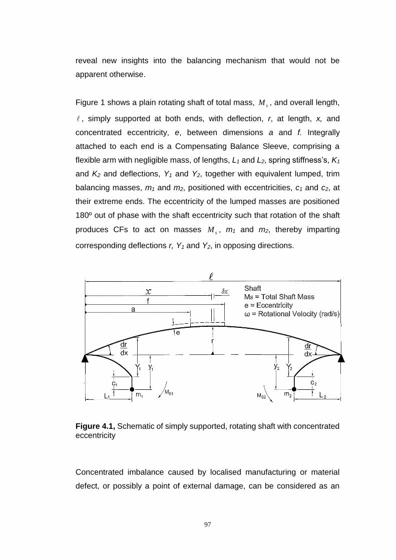
97
reveal new insights into the balancing mechanism that would not be
apparent otherwise.
Figure 1 shows a plain rotating shaft of total mass, sM , and overall length,
, simply supported at both ends, with deflection, r, at length, x, and
concentrated eccentricity, e, between dimensions a and f. Integrally
attached to each end is a Compensating Balance Sleeve, comprising a
flexible arm with negligible mass, of lengths, L1 and L2, spring stiffness’s, K1
and K2 and deflections, Y1 and Y2, together with equivalent lumped, trim
balancing masses, m1 and m2, positioned with eccentricities, c1 and c2, at
their extreme ends. The eccentricity of the lumped masses are positioned
180º out of phase with the shaft eccentricity such that rotation of the shaft
produces CFs to act on masses sM , m1 and m2, thereby imparting
corresponding deflections r, Y1 and Y2, in opposing directions.
Figure 4.1, Schematic of simply supported, rotating shaft with concentrated eccentricity
Concentrated imbalance caused by localised manufacturing or material
defect, or possibly a point of external damage, can be considered as an
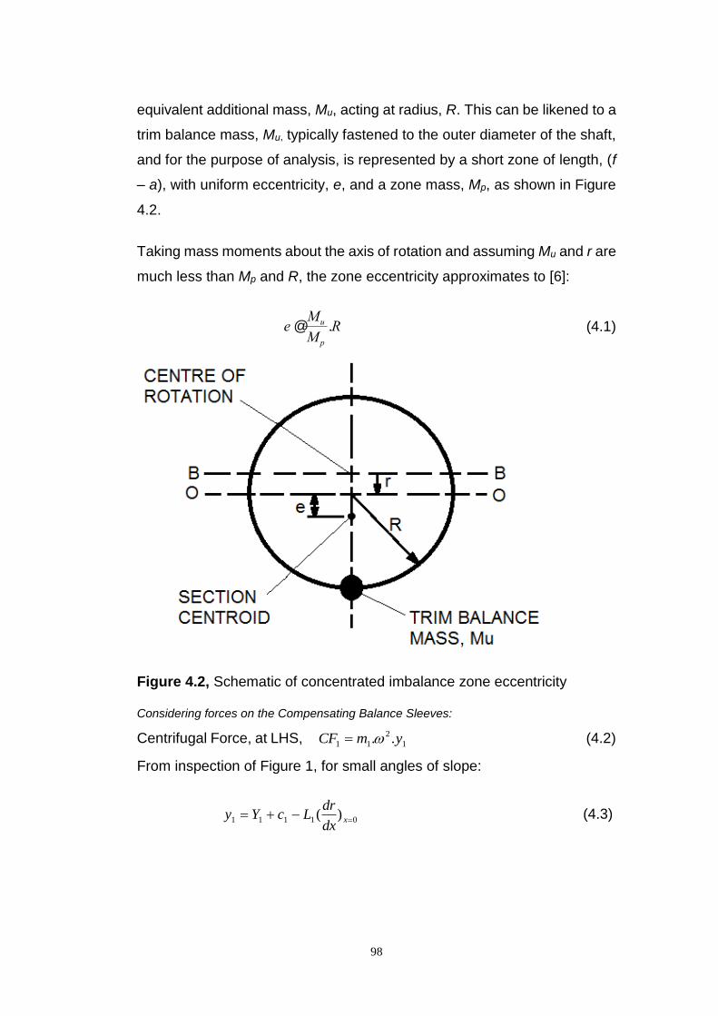
98
equivalent additional mass, Mu, acting at radius, R. This can be likened to a
trim balance mass, Mu, typically fastened to the outer diameter of the shaft,
and for the purpose of analysis, is represented by a short zone of length, (f
– a), with uniform eccentricity, e, and a zone mass, Mp, as shown in Figure
4.2.
Taking mass moments about the axis of rotation and assuming Mu and r are
much less than Mp and R, the zone eccentricity approximates to [6]:
e @Mu
M p
.R (4.1)
Figure 4.2, Schematic of concentrated imbalance zone eccentricity Considering forces on the Compensating Balance Sleeves:
Centrifugal Force, at LHS, 1
2
11 .. ymCF (4.2)
From inspection of Figure 1, for small angles of slope:
01111 )( xdx
drLcYy
(4.3)
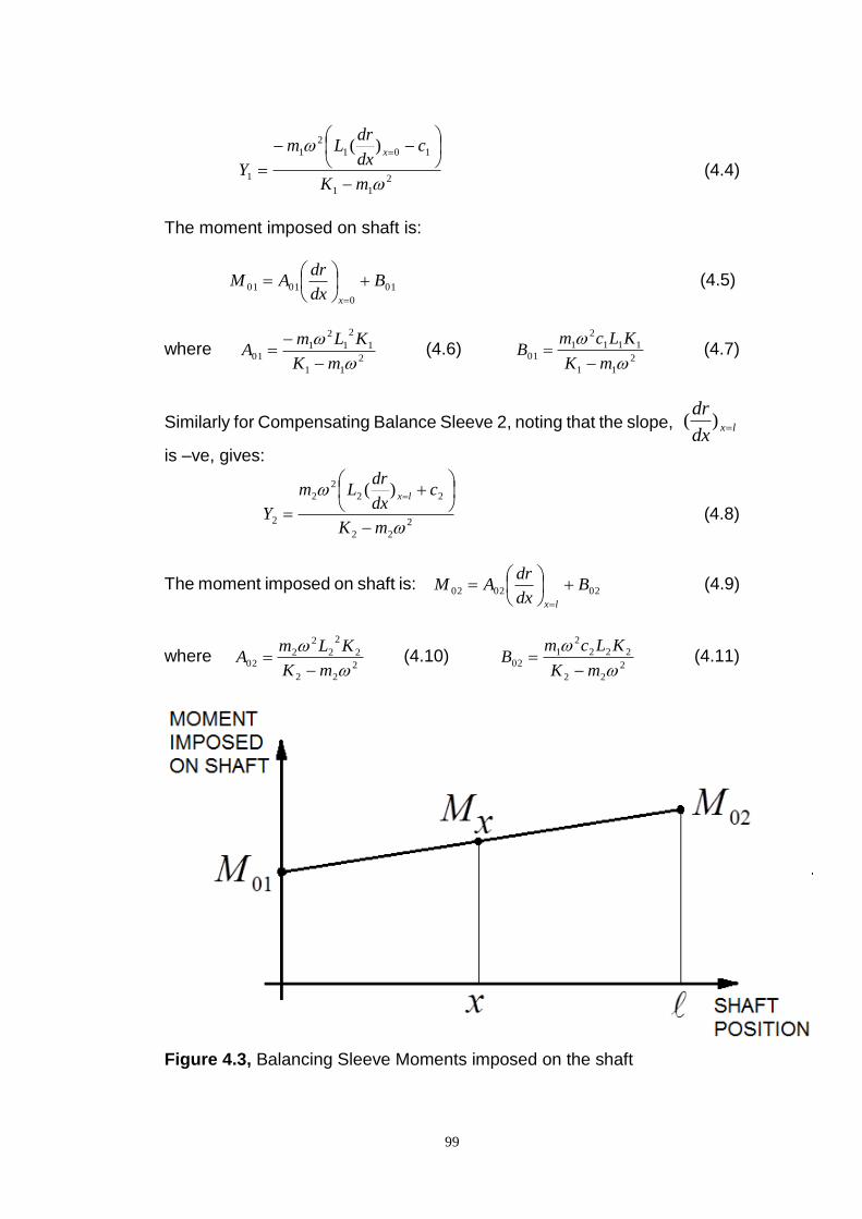
99
2
11
101
2
1
1
)(
mK
cdx
drLm
Y
x
(4.4)
The moment imposed on shaft is:
01
0
0101 Bdx
drAM
x
(4.5)
where 2
11
1
2
1
2
101
mK
KLmA
(4.6)
2
11
111
2
101
mK
KLcmB
(4.7)
Similarly for Compensating Balance Sleeve 2, noting that the slope, lxdx
dr)(
is –ve, gives:
2
22
22
2
2
2
)(
mK
cdx
drLm
Ylx
(4.8)
The moment imposed on shaft is: 020202 B
dx
drAM
lx
(4.9)
where 2
22
2
2
2
2
202
mK
KLmA
(4.10)
2
22
222
2
102
mK
KLcmB
(4.11)
Figure 4.3, Balancing Sleeve Moments imposed on the shaft
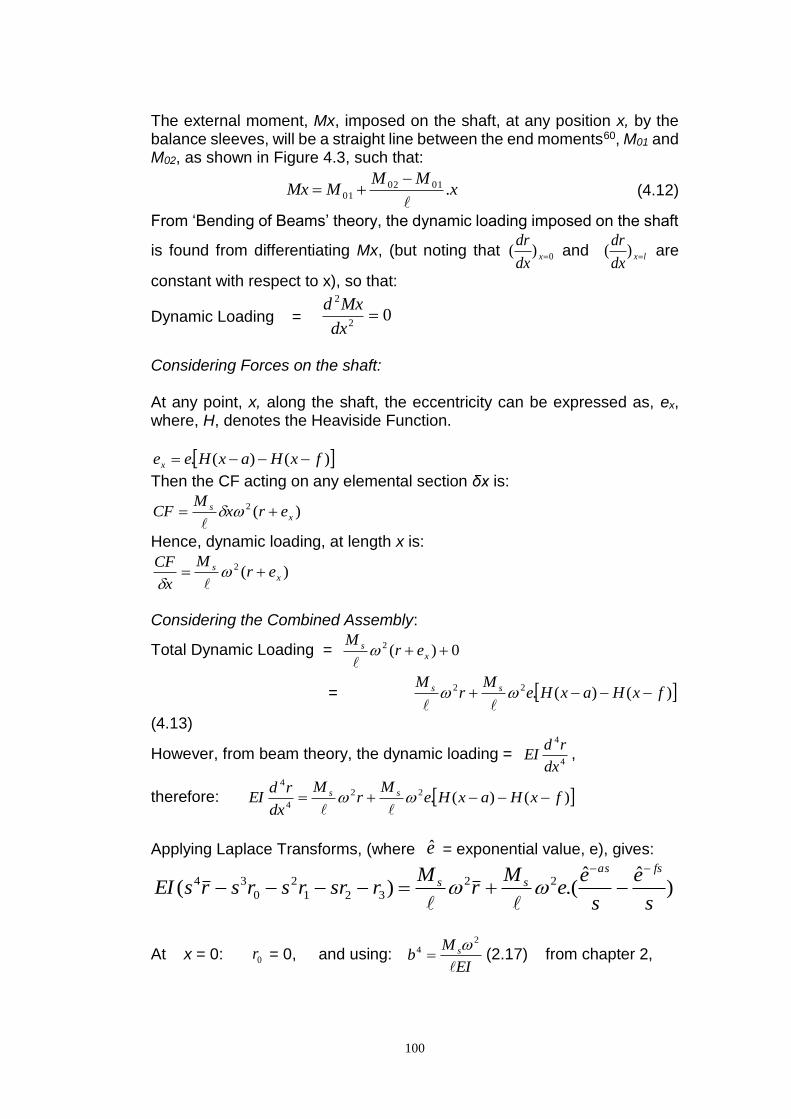
100
The external moment, Mx, imposed on the shaft, at any position x, by the balance sleeves, will be a straight line between the end moments60, M01 and M02, as shown in Figure 4.3, such that:
xMM
MMx .010201
(4.12)
From ‘Bending of Beams’ theory, the dynamic loading imposed on the shaft
is found from differentiating Mx, (but noting that 0)( xdx
dr and lx
dx
dr)( are
constant with respect to x), so that:
Dynamic Loading = 02
2
dx
Mxd
Considering Forces on the shaft: At any point, x, along the shaft, the eccentricity can be expressed as, ex, where, H, denotes the Heaviside Function.
)()(. fxHaxHeex
Then the CF acting on any elemental section δx is:
)(2
xs erx
MCF
Hence, dynamic loading, at length x is:
)(2
xs er
M
x
CF
Considering the Combined Assembly:
Total Dynamic Loading = 0)(2 xs er
M
= )()(.22 fxHaxHeM
rM ss
(4.13)
However, from beam theory, the dynamic loading = 4
4
dx
rdEI ,
therefore: )()(.22
4
4
fxHaxHeM
rM
dx
rdEI ss
Applying Laplace Transforms, (where e = exponential value, e), gives:
)ˆˆ
.()( 22
321
2
0
34
s
e
s
ee
Mr
MrsrrsrsrsEI
fsas
ss
At x = 0: 0r = 0, and using: EI
Mb s
24
(2.17) from chapter 2,
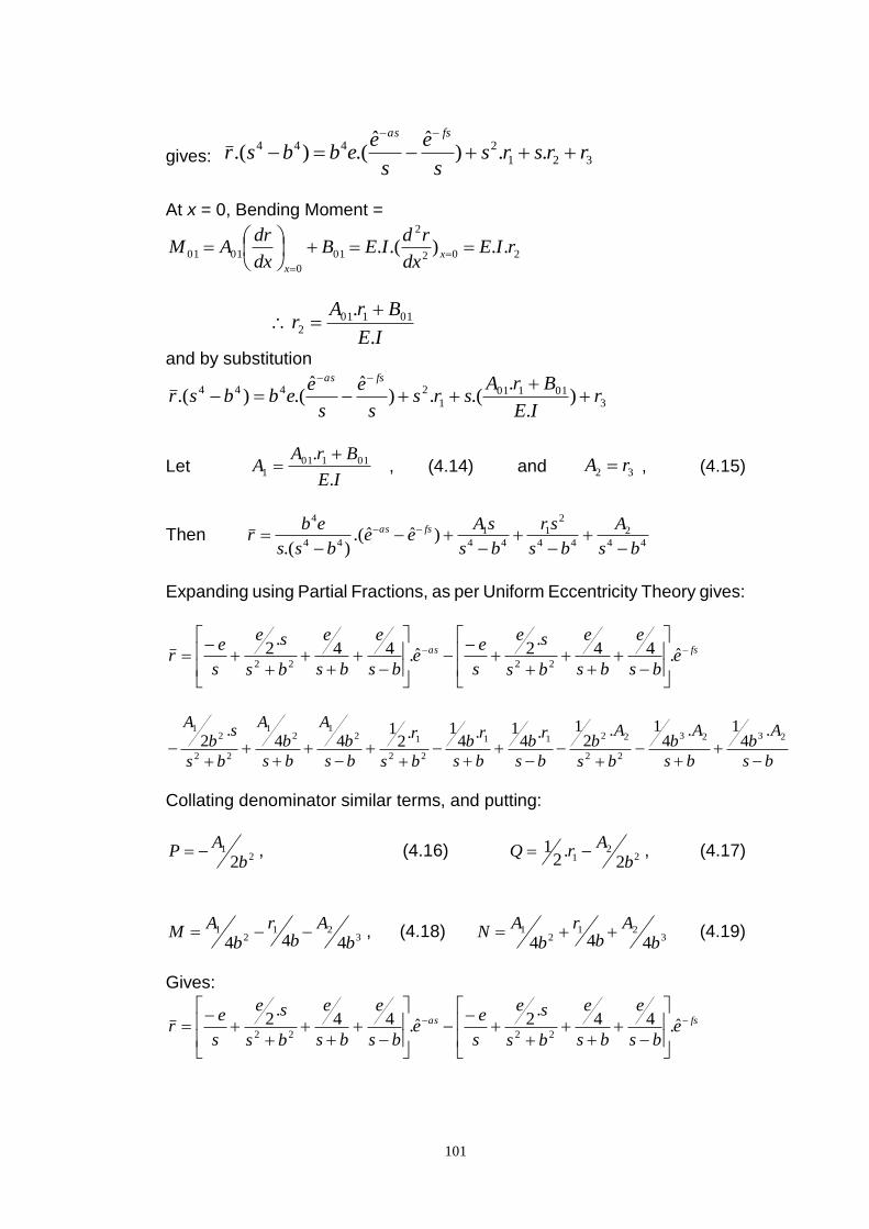
101
gives: 321
2444 ..)ˆˆ
.().( rrsrss
e
s
eebbsr
fsas
At x = 0, Bending Moment =
202
2
01
0
0101 ..).(. rIEdx
rdIEB
dx
drAM x
x
IE
BrAr
.
. 011012
and by substitution
301101
1
2444 ).
..(.)
ˆˆ.().( r
IE
BrAsrs
s
e
s
eebbsr
fsas
Let IE
BrAA
.
. 01101
1
, (4.14) and 32 rA , (4.15)
Then 44
2
44
2
1
44
1
44
4
)ˆˆ.().( bs
A
bs
sr
bs
sAee
bss
ebr fsas
Expanding using Partial Fractions, as per Uniform Eccentricity Theory gives:
fsas ebs
e
bs
e
bs
se
s
ee
bs
e
bs
e
bs
se
s
er
ˆ.44
.2ˆ.44
.2
2222
bs
Ab
bs
Ab
bs
Ab
bs
rb
bs
rb
bs
r
bs
b
A
bs
b
A
bs
sb
A
2323
22
2211
22
121
21
22
21 .
41.
41.
21.
41.
41.
21
44.
2
Collating denominator similar terms, and putting:
21
2b
AP , (4.16) 2
21 2
.2
1b
ArQ , (4.17)
321
21
444 b
Ab
r
b
AM , (4.18) 3
212
1
444 b
Ab
r
b
AN (4.19)
Gives:
fsas ebs
e
bs
e
bs
se
s
ee
bs
e
bs
e
bs
se
s
er
ˆ.44
.2ˆ.44
.2
2222
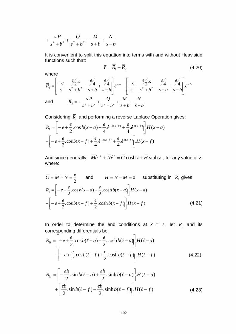
102
bs
N
bs
M
bs
Q
bs
Ps
2222
.
It is convenient to split this equation into terms with and without Heaviside functions such that:
21 RRr (4.20)
where
fsas ebs
e
bs
e
bs
se
s
ee
bs
e
bs
e
bs
se
s
eR
ˆ.44
.2ˆ.44
.2
22221
and bs
N
bs
M
bs
Q
bs
PsR
22222
.
Considering 1R and performing a reverse Laplace Operation gives:
)(.ˆ.4
ˆ.4
)(cos.2
)()(
1 axHee
ee
axbe
eR axbaxb
)(.ˆ.4
ˆ.4
)(cos.2
)()( fxHee
ee
fxbe
e fxbfxb
And since generally, zHzGeNeM zz sinhcoshˆˆ , for any value of z,
where:
2
eNMG and 0 MNH substituting in 1R gives:
)(.)(cosh.2
)(cos.2
1 axHaxbe
axbe
eR
)(.)(cosh.2
)(cos.2
fxHfxbe
fxbe
e
(4.21)
In order to determine the end conditions at x = , let 1R and its
corresponding differentials be:
)(.)(cosh.2
)(cos.2
1 aHabe
abe
eR l
)(.)(cosh.2
)(cos.2
fHfbe
fbe
e
(4.22)
)(.)(sinh.2
)(sin.2
1 aHabeb
abeb
R l
)(.)(sinh.2
)(sin.2
fHfbeb
fbeb
(4.23)
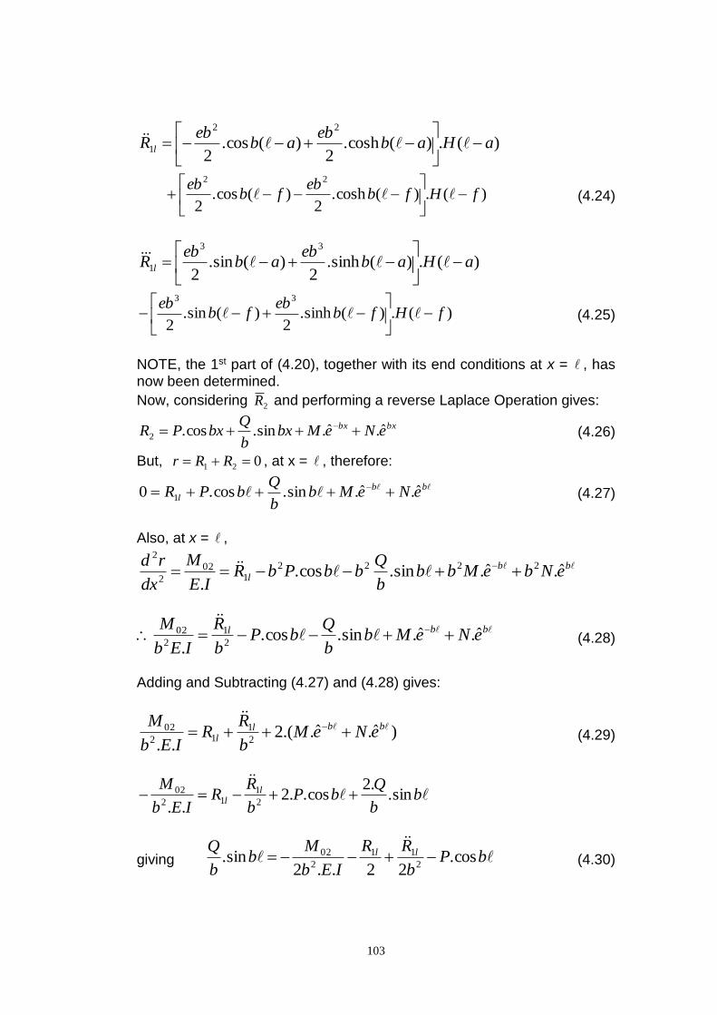
103
)(.)(cosh.2
)(cos.2
22
1 aHabeb
abeb
R l
)(.)(cosh.2
)(cos.2
22
fHfbeb
fbeb
(4.24)
)(.)(sinh.2
)(sin.2
33
1 aHabeb
abeb
R l
)(.)(sinh.2
)(sin.2
33
fHfbeb
fbeb
(4.25)
NOTE, the 1st part of (4.20), together with its end conditions at x = , has now been determined.
Now, considering 2R and performing a reverse Laplace Operation gives:
bxbx eNeMbxb
QbxPR ˆ.ˆ.sin.cos.2
(4.26)
But, 021 RRr , at x = , therefore:
bb
l eNeMbb
QbPR ˆ.ˆ.sin.cos.0 1
(4.27)
Also, at x = ,
bb
l eNbeMbbb
QbbPbR
IE
M
dx
rdˆ.ˆ.sin.cos.
.
2222
102
2
2
bbl eNeMbb
QbP
b
R
IEb
Mˆ.ˆ.sin.cos.
. 2
1
2
02 (4.28)
Adding and Subtracting (4.27) and (4.28) gives:
)ˆ.ˆ..(2.. 2
112
02
bbll eNeM
b
RR
IEb
M
(4.29)
bb
QbP
b
RR
IEb
M ll sin.
.2cos..2
.. 2
112
02
giving
bPb
RR
IEb
Mb
b
Q ll cos.22..2
sin.2
11
2
02 (4.30)
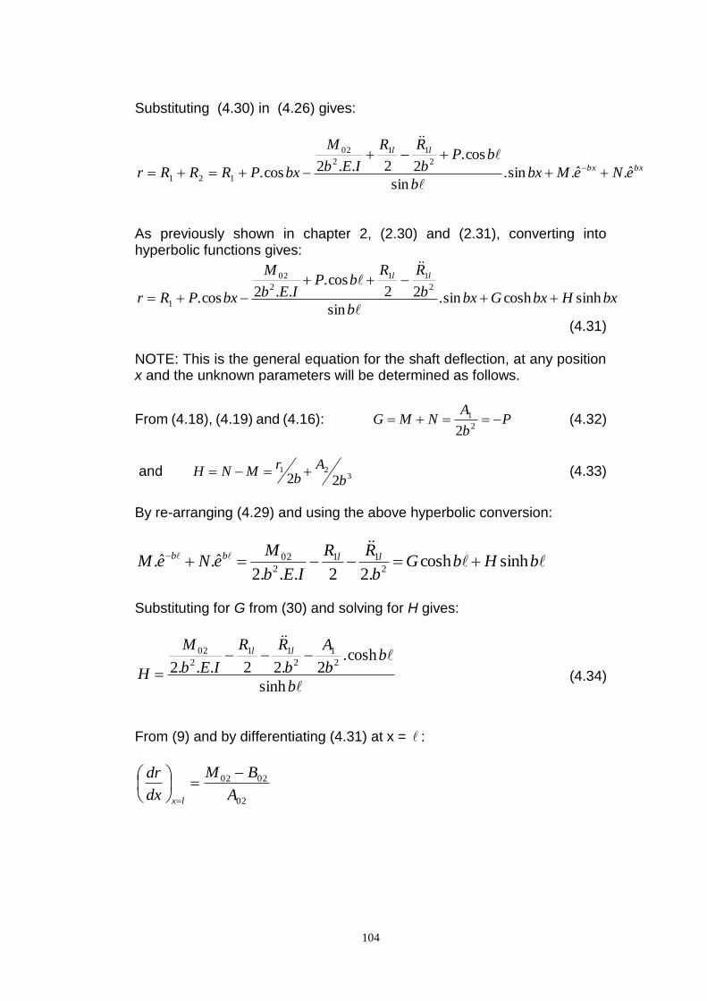
104
Substituting (4.30) in (4.26) gives:
bxbx
ll
eNeMbxb
bPb
RR
IEb
M
bxPRRRr ˆ.ˆ.sin.sin
cos.22..2cos.
2
11
2
02
121
As previously shown in chapter 2, (2.30) and (2.31), converting into hyperbolic functions gives:
bxHbxGbxb
b
RRbP
IEb
M
bxPRr
ll
sinhcoshsin.sin
22cos.
..2cos.2
11
2
02
1
(4.31) NOTE: This is the general equation for the shaft deflection, at any position x and the unknown parameters will be determined as follows.
From (4.18), (4.19) and (4.16): Pb
ANMG
2
1
2 (4.32)
and 321
22 b
Ab
rMNH (4.33)
By re-arranging (4.29) and using the above hyperbolic conversion:
bHbGb
RR
IEb
MeNeM llbb sinhcosh
.22...2ˆ.ˆ.
2
11
2
02
Substituting for G from (30) and solving for H gives:
b
bb
A
b
RR
IEb
M
H
ll
sinh
cosh.2.22...2 2
1
2
11
2
02
(4.34)
From (9) and by differentiating (4.31) at x = :
02
0202
A
BM
dx
dr
lx
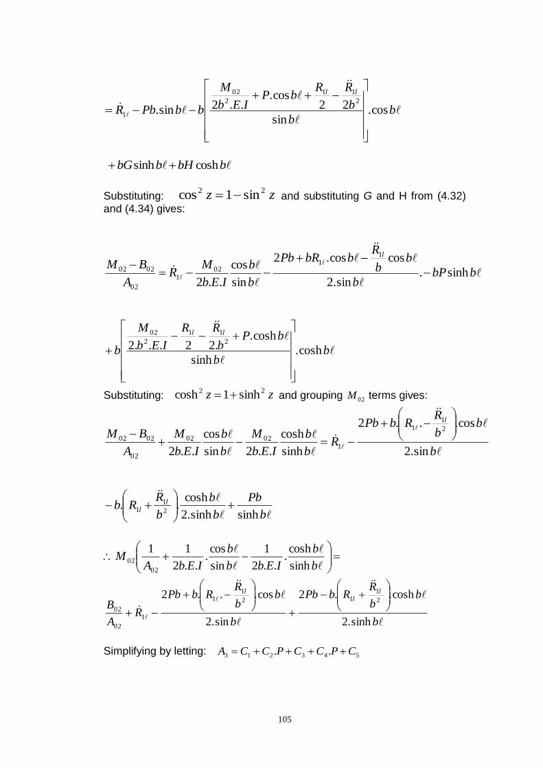
105
b
b
b
RRbP
IEb
M
bbPbR
ll
cos.sin
22cos.
..2sin.2
11
2
02
1
bbHbbG coshsinh
Substituting: zz 22 sin1cos and substituting G and H from (4.32) and (4.34) gives:
bbPb
bb
RbbRPb
b
b
IEb
MR
A
BMl
sinh.sin.2
coscos.2
sin
cos
..2
11
021
02
0202
bb
bPb
RR
IEb
M
b
ll
cosh.sinh
cosh..22...2 2
11
2
02
Substituting: zz 22 sinh1cosh and grouping 02M terms gives:
b
bb
RRbPb
Rb
b
IEb
M
b
b
IEb
M
A
BM
l
sin.2
cos...2
sinh
cosh
..2sin
cos
..2
2
11
10202
02
0202
b
Pb
b
b
b
RRb l
lsinhsinh.2
cosh..
2
11
b
b
IEbb
b
IEbAM
sinh
cosh.
..2
1
sin
cos.
..2
11
02
02
b
bb
RRbPb
b
bb
RRbPb
RA
B
ll
l
sinh.2
cosh..2
sin.2
cos...22
112
11
1
02
02
Simplifying by letting: 543213 .. CPCCPCCA

106
where:
1
02
02
1 RA
BC (4.35),
b
bC
sin2 (4.36),
b
bb
RR
bC
l
sin.2
cos..
.
2
11
3
(4.37)
b
bC
sinh4 (4.38),
b
bb
RR
bC
l
sinh.2
cosh..
.
2
1
1
5
(4.39)
426 CCC (4.40), 5317 CCCC (4.41)
Let:
b
b
IEbb
b
IEbAA
sinh
cosh.
..2
1
sin
cos.
..2
11
02
4 (4.42)
4
76
4
302
.
A
CCP
A
AM
(4.43)
By differentiating (4.31) and noting that 01 R at x = 0
Hbb
b
RRbP
IEb
M
brdx
drll
x
.sin
22cos.
..2.2
11
2
02
1
0
(4.44)
Combining (4.14) and (4.16) and re-arranging gives:
01
01
2
1
2
A
BEIPbr
and substituting in (4.44) together with H from (4.34)
gives:
b
b
RRbP
IEb
M
bA
BPIEbll
sin
22cos.
..2....2 2
11
2
02
01
01
2
b
bPb
RR
IEb
M
b
ll
sinh
cosh..22...2.
2
11
2
02
107
b
b
RRbP
bbIEbbIEb
MA
BPIEbll
sin
.22cos.
.sin...2
1
sinh...2
1.
...2 2
11
02
01
01
2
b
b
RRbP
b
ll
sinh
.22cosh.
.2
11
Simplifying by letting: 765402321 .... DPDDPDMDDPD (4.45)
where: 01
2
1
...2
A
PIEbD (4.46),
01
01
2A
BD (4.47)
bIEbbIEbD
sin...2
1
sinh...2
13 (4.48),
b
bbD
sin
cos.4 (4.49)
b
b
RR
bD
ll
sin
.22.2
11
5
(4.50),
b
bbD
sinh
cosh.6 (4.51)
b
b
RR
bD
ll
sinh
.22.2
11
7
(4.52)
3
641
8D
DDDD
(4.53),
3
752
9D
DDDD
(4.54)
98
3
752
3
641
02 .. DDPD
DDD
D
DDDPM
(4.55)
Equating (4.43) and (4.55) gives: 98
4
76 ..
DDPA
CCP
and hence: 846
794
.
.
DAC
CDAP
(4.56)
Therefore, all the unknown parameters P, M02, G and H, required to
calculate the shaft deflection, for any position x, from equation (4.31), can
now be determined from (4.56), (4.55), (4.32) and (4.34).
108
To determine the Reaction Loads, from beam theory, the vertical shear
force within the beam caused by bending is given by: 3
3
dx
rdEISFv
At x = 0, from (4.33) and (4.15), 313 2)
2( b
br
Hr (4.57)
and at x = , by differentiating (4.31)
bb
b
RRbP
IEb
M
bbPbRr
ll
cos.sin
22cos.
..2.sin.2
11
2
02
33
1
bHbbGb coshsinh 33 (4.58)
which is solvable knowing 1R from (4.25).
Finally, the total reaction force applied to the supports equals internal shear
force + external spring force applied by the Compensating Balance Sleeve.
At x = 0: 1131 ...Re YKrIE (4.59)
and at x = , 222 ...Re YKrIE (4.60)
(note: shear force is –ve at RHS).
The system is now fully determined and numerical analysis is possible by
inserting the above equations into a suitable analytical computer
programme.
4.3 Eliminating/ Nullifying the Impact of the 1st Critical Speed
From (4.31):
bxHbxGbxb
b
RRbP
IEb
M
bxPRr
ll
sinhcoshsin.sin
22cos.
..2cos.2
11
2
02
1
109
it can be seen that shaft displacement, r, becomes infinite, thereby
identifying the critical speeds, when 0sin b , i.e. when b , 2 , 3
etc., thereby defining the first critical frequency as M
EIcrit
.)( 2
.
To avoid the singularity, the 3rd term numerator can also be made equal to
zero, at b , by substitution of P, (4.16), A1, (4.14) and M01, (4.5) to give:
022..2..2 2
11
2
01
2
02
b
RR
IEb
M
IEb
M ll
(4.61)
But, from (4.22) and (4.24) and for both )( a and )( f >0:
.)(cosh.2
)(cosh.2
)(cos.2
)(cos.2
.2
1
22 2
11
ab
eab
eab
eab
ee
b
RR ll
)(cosh.
2)(cosh.
2)(cos.
2)(cos.
2.
2
1fb
efb
efb
efb
ee
Hence, )(cos.2
)(cos.222 2
11 fbe
abe
b
RR ll
(4.61a)
and, through the application of trigonometric substitution:
bfbbfbbabbabe
b
RR ll sin.sincos.cossin.sincos.cos.222 2
11
.
At, b , kebfbae
b
RR ll .coscos.222 2
11
(4.62)
By defining a Concentrated Imbalance Coefficient as:
2
coscos bfbak
(4.63)
and substituting into (4.61) gives: 0...2..2 2
01
2
02
ke
IEb
M
IEb
M
therefore
M01 +M02 = -e.k.2b2.E.I = -2.k. b2.E.I.e( ) (4.64)
110
This equation provides the requirements for balance sleeve compensation
to enable elimination, (more exactly, move to a higher speed), of the 1st
critical frequency of a simply supported shaft with concentrated imbalance.
In the case of uniform eccentricity, chapter 2, the requirement for “classical”
critical speed elimination, (corresponding to b ), determined that both
balancing sleeve moments are
Mo = b2.EI.e. Comparing with the case for
concentrated imbalance, the requirement is seen to be a fixed portion of the
same equation since the Concentrated Imbalance Coefficient, k will be a
constant for given values of a and f, as also shown graphically in Figure
4.4.
It is also seen that k is an absolute maximum when 0a and f , giving
1k , i.e. the condition of uniform eccentricity. Under such conditions,
from (4.64):
MoeEIbMM .2...2 2
0201 , thereby providing a direct correlation
between the analysis for concentrated imbalance and that for uniform
eccentricity.
Figure 4.4, Zone of concentrated imbalance
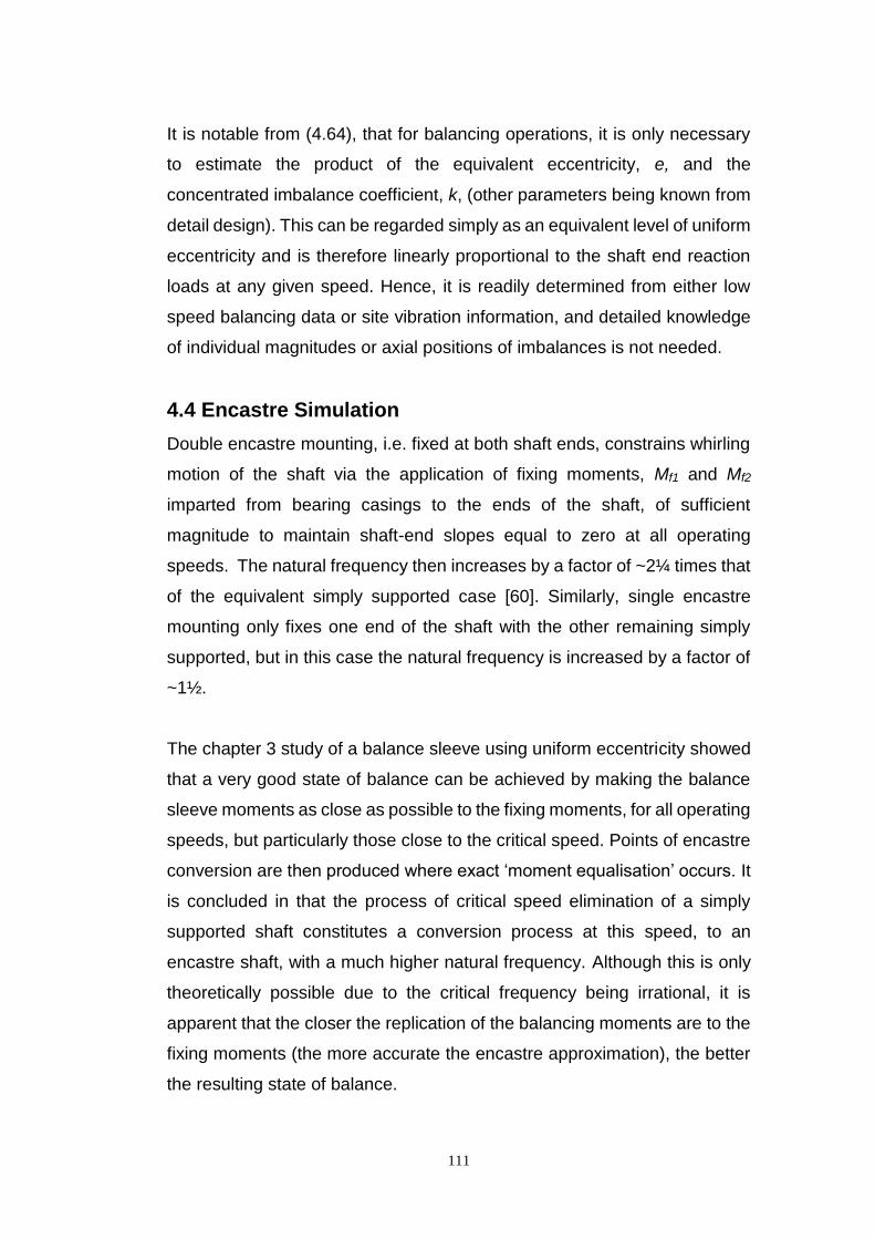
111
It is notable from (4.64), that for balancing operations, it is only necessary
to estimate the product of the equivalent eccentricity, e, and the
concentrated imbalance coefficient, k, (other parameters being known from
detail design). This can be regarded simply as an equivalent level of uniform
eccentricity and is therefore linearly proportional to the shaft end reaction
loads at any given speed. Hence, it is readily determined from either low
speed balancing data or site vibration information, and detailed knowledge
of individual magnitudes or axial positions of imbalances is not needed.
4.4 Encastre Simulation
Double encastre mounting, i.e. fixed at both shaft ends, constrains whirling
motion of the shaft via the application of fixing moments, Mf1 and Mf2
imparted from bearing casings to the ends of the shaft, of sufficient
magnitude to maintain shaft-end slopes equal to zero at all operating
speeds. The natural frequency then increases by a factor of ~2¼ times that
of the equivalent simply supported case [60]. Similarly, single encastre
mounting only fixes one end of the shaft with the other remaining simply
supported, but in this case the natural frequency is increased by a factor of
~1½.
The chapter 3 study of a balance sleeve using uniform eccentricity showed
that a very good state of balance can be achieved by making the balance
sleeve moments as close as possible to the fixing moments, for all operating
speeds, but particularly those close to the critical speed. Points of encastre
conversion are then produced where exact ‘moment equalisation’ occurs. It
is concluded in that the process of critical speed elimination of a simply
supported shaft constitutes a conversion process at this speed, to an
encastre shaft, with a much higher natural frequency. Although this is only
theoretically possible due to the critical frequency being irrational, it is
apparent that the closer the replication of the balancing moments are to the
fixing moments (the more accurate the encastre approximation), the better
the resulting state of balance.

112
To confirm that these conditions also apply to the more generalised case of
a single concentrated imbalance, equivalent double and single encastre
shafts have been analysed. By applying a similar analytical methodology to
that used in chapter 3, but with boundary conditions set such that the shaft
end slope or bending moment is zero, for appropriate encastre or simply
supported ends, the equation for shaft deflection becomes:
)sinh.(sin)cosh.(cos1 bxbxb
QbxbxPRr e
ee (4.65)
for both double and single encastre cases, where the suffix e denotes the
encastre condition,
bb
bbb
RbbR
P
ll
ecosh.cos.22
)sinh.(sin)cosh.(cos 11
, double encastre (4.66)
bbbb
bbb
RbbR
P
ll
esinh.cos.2cosh.sin.2
)sinh.(sin)sinh.(sin2
11
, single encastre
bb
bbRbbRbQ ll
ecosh.cos.22
)cosh.(cos)sinh.(sin. 11
, double encastre (4.67)
bbbb
bbb
RbbRb
Q
l
l
ecosh.sin.2sinh.cos.2
)cosh.(cos)cosh.(cos. 1
1
, single encastre
The double- and single-encastre denominators of eP and eQ , become zero
and represent the 1st critical speed of the system as r ∞, when 73.4b
radians and 93.3b radians, respectively. Comparing these results with
the simply supported case, the critical speeds are correspondingly 2.27 and
1.56 times greater.

113
Further analysis gives the corresponding fixing moments as:
IEPbM ef ...2 2
1 , )sin...2cos..2..(. 2
1
2
12 bQbbPbRbRIEM eellf ,
for double encastre, and
IEPbM ef ...2 2
1 , 02 fM , for single encastre mounting (4.68)
Notably, for a speed corresponding to b , the sum of the fixing moment
reduces to:
IEbkeMM ff ..2.. 2
21 , for both cases (4.69)
which is identical to the moment requirement for elimination of the simply
supported system, given by (4.64). Hence, moment equalisation occurs
producing encastre conversion and the critical speed is theoretically
eliminated. This is illustrated graphically in Figure 4.5 through use of a case
study of both sets of moments, (set close to optimum balance
compensation), using the site equivalent parameter values, shown in Table
4.1, for a Siemens sub-15MW gas turbine compressor. Note, for
comparison purposes, these are slightly modified versions of the
parameters given in Table 2.1, chapter 2, to take account of the change
from uniform eccentricity to a single concentrated eccentric zone. It can be
seen that the characteristic curves intersect at the classical critical speed,
(11,902 rpm, given by b ) and that only a small moment spike is evident
in the vicinity.
From beam theory, the encastre shaft end reaction loads are given by:
31 ..Re ee rIE where 2
3 ..2 bQr ee
and ee rIE ..Re 2 , (shear force –ve at RHS)
where bbQbbbPbRr eele sinhcos..coshsin... 23
1
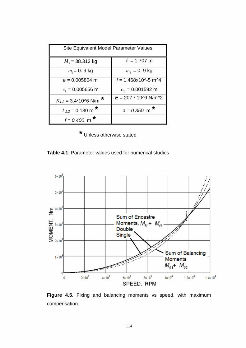
114
* Unless otherwise stated
Table 4.1. Parameter values used for numerical studies
Figure 4.5. Fixing and balancing moments vs speed, with maximum
compensation.
Site Equivalent Model Parameter Values
sM = 38.312 kg = 1.707 m
1m = 0. 9 kg 2m = 0. 9 kg
e = 0.005804 m I = 1.468x10^-5 m^4
1c = 0.005656 m 2c = 0.001592 m
K1,2 = 3.4ˣ10^6 N/m * E = 207 ˣ 10^9 N/m^2
L1,2 = 0.130 m * a = 0.350 m *
f = 0.400 m *
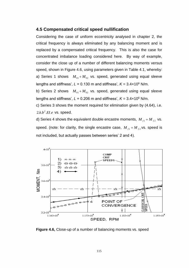
115
4.5 Compensated critical speed nullification
Considering the case of uniform eccentricity analysed in chapter 2, the
critical frequency is always eliminated by any balancing moment and is
replaced by a compensated critical frequency. This is also the case for
concentrated imbalance loading considered here. By way of example,
consider the close up of a number of different balancing moments versus
speed, shown in Figure 4.6, using parameters given in Table 4.1, whereby:
a) Series 1 shows 0201 MM vs. speed, generated using equal sleeve
lengths and stiffness’, L = 0.130 m and stiffness’, K = 3.4×10⁶ N/m.
b) Series 2 shows 0201 MM vs. speed, generated using equal sleeve
lengths and stiffness’, L = 0.206 m and stiffness’, K = 3.4×10⁶ N/m.
c) Series 3 shows the moment required for elimination given by (4.64), i.e.
eEIbk ....2 2 vs. speed.
d) Series 4 shows the equivalent double encastre moments, 21 ff MM vs.
speed. (note: for clarity, the single encastre case, 21 ff MM vs. speed is
not included, but actually passes between series’ 2 and 4).
Figure 4.6, Close-up of a number of balancing moments vs. speed
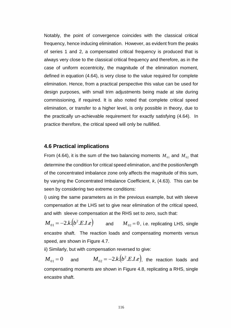
116
Notably, the point of convergence coincides with the classical critical
frequency, hence inducing elimination. However, as evident from the peaks
of series 1 and 2, a compensated critical frequency is produced that is
always very close to the classical critical frequency and therefore, as in the
case of uniform eccentricity, the magnitude of the elimination moment,
defined in equation (4.64), is very close to the value required for complete
elimination. Hence, from a practical perspective this value can be used for
design purposes, with small trim adjustments being made at site during
commissioning, if required. It is also noted that complete critical speed
elimination, or transfer to a higher level, is only possible in theory, due to
the practically un-achievable requirement for exactly satisfying (4.64). In
practice therefore, the critical speed will only be nullified.
4.6 Practical implications
From (4.64), it is the sum of the two balancing moments 01M and 02M that
determine the condition for critical speed elimination, and the position/length
of the concentrated imbalance zone only affects the magnitude of this sum,
by varying the Concentrated Imbalance Coefficient, k, (4.63). This can be
seen by considering two extreme conditions:
i) using the same parameters as in the previous example, but with sleeve
compensation at the LHS set to give near elimination of the critical speed,
and with sleeve compensation at the RHS set to zero, such that:
eIEbkM .....2 2
01 and 002 M , i.e. replicating LHS, single
encastre shaft. The reaction loads and compensating moments versus
speed, are shown in Figure 4.7.
ii) Similarly, but with compensation reversed to give:
001 M and eIEbkM .....2 2
02 , the reaction loads and
compensating moments are shown in Figure 4.8, replicating a RHS, single
encastre shaft.
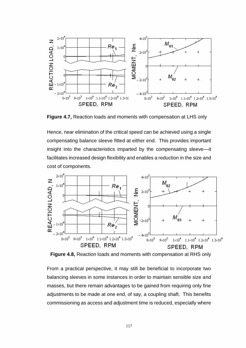
117
Figure 4.7, Reaction loads and moments with compensation at LHS only
Hence, near elimination of the critical speed can be achieved using a single
compensating balance sleeve fitted at either end. This provides important
insight into the characteristics imparted by the compensating sleeve—it
facilitates increased design flexibility and enables a reduction in the size and
cost of components.
Figure 4.8, Reaction loads and moments with compensation at RHS only
From a practical perspective, it may still be beneficial to incorporate two
balancing sleeves in some instances in order to maintain sensible size and
masses, but there remain advantages to be gained from requiring only fine
adjustments to be made at one end, of say, a coupling shaft. This benefits
commissioning as access and adjustment time is reduced, especially where
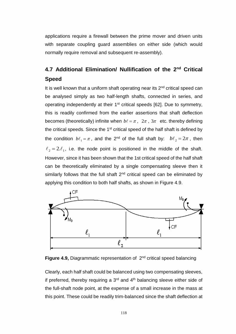
118
applications require a firewall between the prime mover and driven units
with separate coupling guard assemblies on either side (which would
normally require removal and subsequent re-assembly).
4.7 Additional Elimination/ Nullification of the 2nd Critical
Speed
It is well known that a uniform shaft operating near its 2nd critical speed can
be analysed simply as two half-length shafts, connected in series, and
operating independently at their 1st critical speeds [62]. Due to symmetry,
this is readily confirmed from the earlier assertions that shaft deflection
becomes (theoretically) infinite when b , 2 , 3 etc. thereby defining
the critical speeds. Since the 1st critical speed of the half shaft is defined by
the condition 1b , and the 2nd of the full shaft by: 22 b , then
12 .2 , i.e. the node point is positioned in the middle of the shaft.
However, since it has been shown that the 1st critical speed of the half shaft
can be theoretically eliminated by a single compensating sleeve then it
similarly follows that the full shaft 2nd critical speed can be eliminated by
applying this condition to both half shafts, as shown in Figure 4.9.
Figure 4.9, Diagrammatic representation of 2nd critical speed balancing
Clearly, each half shaft could be balanced using two compensating sleeves,
if preferred, thereby requiring a 3rd and 4th balancing sleeve either side of
the full-shaft node point, at the expense of a small increase in the mass at
this point. These could be readily trim-balanced since the shaft deflection at
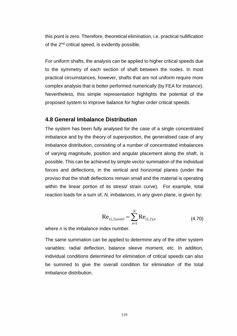
119
this point is zero. Therefore, theoretical elimination, i.e. practical nullification
of the 2nd critical speed, is evidently possible.
For uniform shafts, the analysis can be applied to higher critical speeds due
to the symmetry of each section of shaft between the nodes. In most
practical circumstances, however, shafts that are not uniform require more
complex analysis that is better performed numerically (by FEA for instance).
Nevertheless, this simple representation highlights the potential of the
proposed system to improve balance for higher order critical speeds.
4.8 General Imbalance Distribution
The system has been fully analysed for the case of a single concentrated
imbalance and by the theory of superposition, the generalised case of any
imbalance distribution, consisting of a number of concentrated imbalances
of varying magnitude, position and angular placement along the shaft, is
possible. This can be achieved by simple vector summation of the individual
forces and deflections, in the vertical and horizontal planes (under the
proviso that the shaft deflections remain small and the material is operating
within the linear portion of its stress/ strain curve). For example, total
reaction loads for a sum of, N, imbalances, in any given plane, is given by:
N
n
ntotal
1
),2,1(),2,1( ReRe (4.70)
where n is the imbalance index number. The same summation can be applied to determine any of the other system
variables: radial deflection, balance sleeve moment, etc. In addition,
individual conditions determined for elimination of critical speeds can also
be summed to give the overall condition for elimination of the total
imbalance distribution.

120
4.9 Analytical Results: site equivalent model with a single
offset imbalance
For comparison with chapters 2 and 3, (specific case studies into shafts with
uniform eccentricity), similar numerical examples of concentrated
imbalance loading are now presented, compiled using similar parameter
values, as per Table 4.1. The concentrated zone of imbalance is arbitrarily
chosen to provide offset loading by making, a = 0.350 m and f = 0.400 m.
Figures 4.10 and 4.11 graphically show comparative results from the
numerical calculations, for reaction loads and shaft mid-point deflection. In
both cases the trim balance masses are set to give low speed balance,
resulting in differing trim balance eccentricities, 1c and 2c , due to the offset
nature of shaft imbalance. Figures 4.10, (a) and (b) show shaft end reaction
loads, 1Re and 2Re , versus speed, for three conditions of balance: firstly,
without any balance sleeve compensation, i.e. both sleeves modelled as
zero length and with extremely high stiffness’, K = 3.4×10¹⁶ N/m. Then, for
two compensated cases with sleeves stiffness’, K = 3.4×10⁶ N/m, and a),
equal length sleeves, L = 0.130 m and b), equal length sleeves, L = 0.206
m, to give near maximum compensation with double encastre replication.
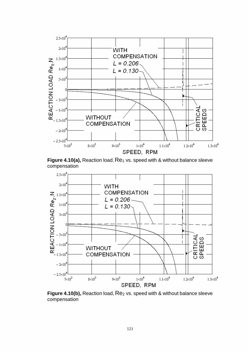
121
Figure 4.10(a), Reaction load, Re1 vs. speed with & without balance sleeve
compensation
Figure 4.10(b), Reaction load, Re2 vs. speed with & without balance sleeve
compensation
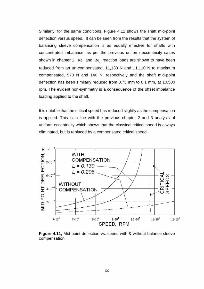
122
Similarly, for the same conditions, Figure 4.11 shows the shaft mid-point
deflection versus speed. It can be seen from the results that the system of
balancing sleeve compensation is as equally effective for shafts with
concentrated imbalance, as per the previous uniform eccentricity cases
shown in chapter 2. 1Re and 2Re reaction loads are shown to have been
reduced from an un-compensated, 11,130 N and 11,110 N to maximum
compensated, 570 N and 140 N, respectively and the shaft mid-point
deflection has been similarly reduced from 0.75 mm to 0.1 mm, at 10,500
rpm. The evident non-symmetry is a consequence of the offset imbalance
loading applied to the shaft.
It is notable that the critical speed has reduced slightly as the compensation
is applied. This is in line with the previous chapter 2 and 3 analysis of
uniform eccentricity which shows that the classical critical speed is always
eliminated, but is replaced by a compensated critical speed.
Figure 4.11, Mid-point deflection vs. speed with & without balance sleeve compensation
123
4.10 Preliminary Conclusions
Chapter 4 extends the special case study – analysis of uniform eccentricity
given in chapters 2 and 3, - to demonstrate the suitability of the new
methodology for the generalised condition of shaft loading with a single
concentrated imbalance. By extension, it is shown that the principle of
superposition allows for more practical imbalance distributions to be
analysed by the process of vector addition of any number of individual
concentrated imbalances, of various magnitude/ position. Further, the
analysis reveals that a series of concentrated imbalances can be regarded
simply as an equivalent level of uniform eccentricity, hence the previous
conclusions developed in chapters 2 and 3 apply equally to this generalised
case of imbalance loading.
The study shows that the nullification of critical speeds is dependent not on
individual discrete values of the balancing moments applied by the
balancing sleeves, but on the sum of those moments; the position or size of
the imbalance only determining the required magnitude of the sum. Hence,
nullification can be achieved by the use of a single compensating balance
sleeve fitted at either end of the shaft, thereby replicating a single encastre
shaft. Alternatively, it is only necessary to make balance corrections at one
end, thereby reducing commissioning and site maintenance times.
It is also illustrated that by extending this concept to counter the mode shape
of the 2nd critical speed, that nullification of this, and to a lesser extent
higher orders, is possible.
In addition, the system also enables balance corrections to be made at more
accessible positions, closer to the shaft ends, as opposed to the usual
inboard positions where higher masses are located; thereby making it useful
to those industries where maintenance is difficult or even dangerous, as in
some nuclear installations. This will be further enhanced if, as envisaged,
future designs will allow for remote adjustment of the balancing moment.
124
Chapter 5
This chapter introduces a Shear Force Reaction ratio which determines the
effective reduction in the equivalent level of residual eccentricity in a shaft
when subjected to maximum balance sleeve compensation. It also
investigates the possible benefits of applying compensation to higher order
critical speeds by the definition/ determination of a Simulation Ratio.
5.1 Shaft end Reaction Loads
Previous analysis presented in chapters 2 and 3, of plain, simply supported
and encastre mounted shafts with uniform eccentricity, derived the following
equations for shaft end reaction loads.
5.1.1 Simply Supported Shafts
In the case of simply supported shafts, with balance sleeve compensation,
from chapter 2, equation (2.41), the shaft end reaction force was shown to
be the sum of internal shear force and the external spring force applied by
the compensating balance sleeve, giving:
KYEIrss 3Re_ , where shaft derivatives at 0x were defined by
0
1
xdx
drr ,
0
2
2
2
xdx
rdr and
0
3
3
3
xdx
rdr from (2.14), (2.15) and
(2.16).
Further it was determined from (2.42) that: 31
3 2)2
( bb
rHr ,
b
bb
AeIEb
Moe
Hsinh
cosh)..22
(...22
21
2
(2.37) and
bA
bBAebBAeb
bA
bBAebBAeb
rsinh
cosh22
sin
cos22
4
33
4
33
1
(2.39)
where the following parameters are defined as:
2
22
mK
KLmA
(2.10),
EI
BArA
1
1 (2.20), bEI
A2
13 (2.38)
2
2
mK
cLKmB
(2.11),
b
bAAAA
b
bAAAAA
sinh
cosh
sin
cos1 3333
4
(2.40)
125
Also, the balancing sleeve moment was defined by: Bdx
drAM
x
0
0 .
(2.9).
However, for a shaft with zero balance correction, i.e. just a plain shaft with
uniform eccentricity but without balance sleeves, then A, 1A , B, K, Y and
0M are all zero, so that:
14 A and
b
be
Hsinh
)cosh1(2
. Also
b
b
b
bebr
sinh
cosh1
sin
cos1.
21
giving:
b
b
b
bebr
sinh
cosh1
sin
cos1.
2
3
3 (5.1)
hence the shaft end reaction load consists of internal shear only:
b
b
b
bEIebss
sinh
cosh1
sin
cos1.
2Re_
3
(5.2)
5.1.2 Encastre Mounted Shafts
Similarly for the case of encastre mounted shafts the dynamic analysis
provided in chapter 3 produced the following parameter equations (3.9) and
(3.8):
bb
bbbbbbePe
cosh.cos1
sinh.sincoshcosh.coscos1.
2
bb
bebbPJ e
coshcos
sinh)sinh(sin
and from (3.10b), shaft end reaction load, 3Re_ EIren (3.10a),
where, Jbr 3
3 .2
Note, in this case the reaction load consists solely of the shaft’s internal
shear force.
By defining bbT cosh.cos1 and bbS coshcos
and making Pe and J substitutions, gives:

126
S
bbbT
bbST
ebr
sinh.2)sinh.(sinsinh.sin
.3
3 and
S
bbbT
bbST
EIeben
sinh.2)sinh.(sinsinh.sin
.Re_ 3 .
Figure 5.1, Reaction Load, (shear Force only), versus non-dimensional speed The encastre and simply supported reaction loads, (shear force only since
there is zero balance correction), versus non-dimensional speeds are
shown in Figure 5.1, using the same parameter values given in chapter 2,
Table 2.1. It can be seen, that for the encastre shaft, the reaction load is
considerably reduced, especially close to the critical speed.
127
5.2 Shear Force Reaction Ratio
It is apparent that a good indication of the possible benefits of encastre
simulation can be obtained by considering the ratio of the two reaction loads
for both mounting conditions; hence, by defining:
Shear Force Reaction Ratio, 𝑅𝑅 =𝑆.𝑆.𝑅𝑒𝑎𝑐𝑡𝑖𝑜𝑛 𝐹𝑜𝑟𝑐𝑒
𝐸𝑛𝑐𝑎𝑠𝑡𝑟𝑒 𝑅𝑒𝑎𝑐𝑡𝑖𝑜𝑛 𝐹𝑜𝑟𝑐𝑒
gives,
S
bbT
bbSTb
b
b
b
b
en
ssRR
)sinh.(sinsinh.sin
sinh.2
.2
sin
cos1
sinh
cosh1
Re_
Re_
(5.3)
A graphical representation of (5.3) is given in Figure 5.2, which shows the
reaction ratio, RR, versus non-dimensional speed, crit / between 0.5 and
1.0. Notably the ratio increases as the non-dimensional speed approaches
unity, indicating the positive benefit of shaft balancing by encastre
simulation, since the methodology of balance sleeve compensation
becomes more effective at the operating regions where the intensity of shaft
imbalance is normally most severe.
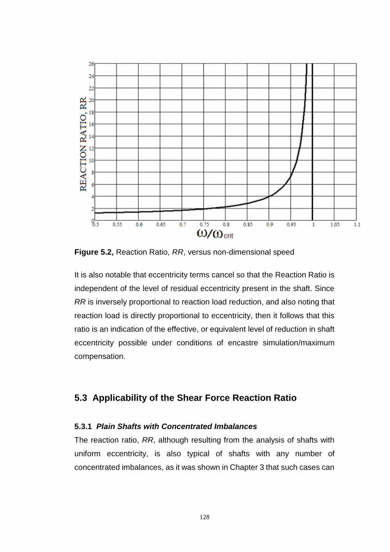
128
Figure 5.2, Reaction Ratio, RR, versus non-dimensional speed
It is also notable that eccentricity terms cancel so that the Reaction Ratio is
independent of the level of residual eccentricity present in the shaft. Since
RR is inversely proportional to reaction load reduction, and also noting that
reaction load is directly proportional to eccentricity, then it follows that this
ratio is an indication of the effective, or equivalent level of reduction in shaft
eccentricity possible under conditions of encastre simulation/maximum
compensation.
5.3 Applicability of the Shear Force Reaction Ratio
5.3.1 Plain Shafts with Concentrated Imbalances
The reaction ratio, RR, although resulting from the analysis of shafts with
uniform eccentricity, is also typical of shafts with any number of
concentrated imbalances, as it was shown in Chapter 3 that such cases can
129
be regarded as an equivalent level of the uniform eccentricity. The following
section now provides further evidence to support this conclusion.
Re-arranging the previous simply supported equation, (5.1), for the
differential term, 3r , for uniform eccentricity, gives:
b
b
b
bebunr
sinh.2
cosh1
sin.2
cos1._ 3
3 (5.4)
Similarly, for a single concentrated shaft imbalance, the previous analysis
of chapter 4, produced equation (4.57), which is written as:
313 2)
2(_ b
br
Hconr (5.5)
Also from chapter 4, (4.34), with zero balance correction making 01M , 02M ,
1A , and P, all equal to zero, gives:
b
b
RR
b
b
RR
H
llll
sinh
.22
sinh
0.22
02
11
2
11
However, from chapter 4, (4.62), at, b , keb
RR ll .22 2
11
where
2
coscos bfbak
, Concentrated Imbalance Coefficient
Hence, lll Rke
b
RR12
11 ..22
and b
RkeH l
sinh
. 1 (5.6)
From chapter 4, (4.22), for positive )( a and )( f :
)(cosh)(cosh)(cos)(cos.2
1 fbabfbabe
R l (5.7)
Considering the hyperbolic terms only and applying trigonometric
substitution:
)sinh(.sinh)cosh(.cosh)(cosh)(cosh abbabbfbab
)sinh(.sinh)cosh(.cosh fbbfbb
)cosh()cosh(.cosh fbabb
)sinh()sinh(.sinh fbabb
130
For operating speeds approaching critical, i.e. 2b , bb sinhcosh ,
and making further trigonometric substitution gives:
)sinh()sinh()cosh()cosh(.cosh fbabfbabb (5.8)
Substituting abfb and expanding gives:
sinh.sinhcosh.cosh)cosh( ababfb
and ababfb cosh.sinhcosh.sinh)sinh(
For a concentrated imbalance where )( ba is relatively small, 0 ,
hence, these terms can be reduced to:
abfb cosh)cosh( and abfb sinh)sinh(
Substituting in (5.8) then gives:
ababababbfbab sinhsinhcoshcosh.cosh)(cosh)(cosh
Hence, 0)(cosh)(cosh fbab
and substituting for the hyperbolic terms in (5.7) gives:
kefbabe
R l .)(cos)(cos.2
1
since from chapter 4, (4.61a), for b ,
kefbab .)(cos)(cos
Substituting in (5.6) then gives: 0sinh
..
b
kekeH
Therefore, from chapter 4, (4.44), 0sin
.00.1
b
kebr
and by substitution in (5.5):
bkebconr
sin
1.._ 3
3 (5.9)
In order to compare the two differential terms, 3r , for the cases of uniform
eccentricity and concentrated imbalance, Figure 5.3 shows a plot of the
bracket terms of equations (5.4) and (5.9) and it can be seen that they are
approximately equal for non-dimensional operating speeds between 0.5
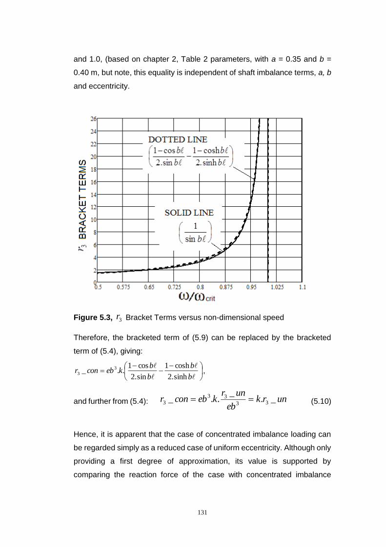
131
and 1.0, (based on chapter 2, Table 2 parameters, with a = 0.35 and b =
0.40 m, but note, this equality is independent of shaft imbalance terms, a, b
and eccentricity.
Figure 5.3, 3r Bracket Terms versus non-dimensional speed
Therefore, the bracketed term of (5.9) can be replaced by the bracketed
term of (5.4), giving:
b
b
b
bkebconr
sinh.2
cosh1
sin.2
cos1.._ 3
3 ,
and further from (5.4): unrkeb
unrkebconr _.
_.._ 33
33
3 (5.10)
Hence, it is apparent that the case of concentrated imbalance loading can
be regarded simply as a reduced case of uniform eccentricity. Although only
providing a first degree of approximation, its value is supported by
comparing the reaction force of the case with concentrated imbalance
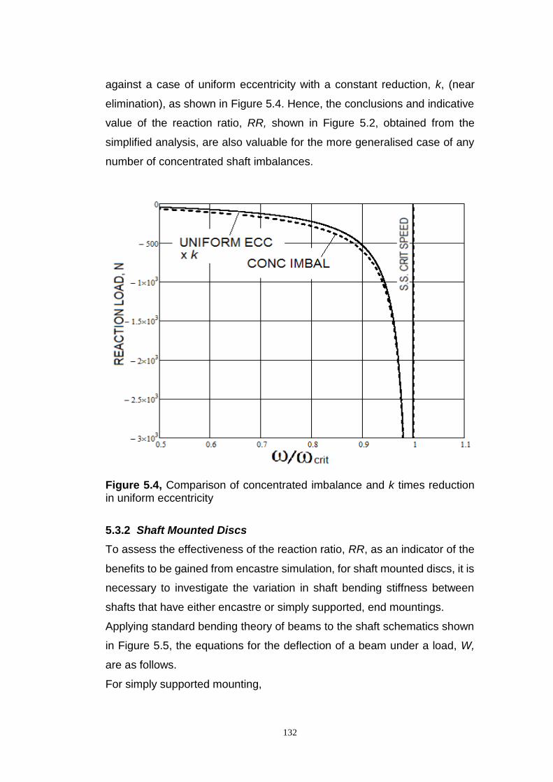
132
against a case of uniform eccentricity with a constant reduction, k, (near
elimination), as shown in Figure 5.4. Hence, the conclusions and indicative
value of the reaction ratio, RR, shown in Figure 5.2, obtained from the
simplified analysis, are also valuable for the more generalised case of any
number of concentrated shaft imbalances.
Figure 5.4, Comparison of concentrated imbalance and k times reduction in uniform eccentricity
5.3.2 Shaft Mounted Discs
To assess the effectiveness of the reaction ratio, RR, as an indicator of the
benefits to be gained from encastre simulation, for shaft mounted discs, it is
necessary to investigate the variation in shaft bending stiffness between
shafts that have either encastre or simply supported, end mountings.
Applying standard bending theory of beams to the shaft schematics shown
in Figure 5.5, the equations for the deflection of a beam under a load, W,
are as follows.
For simply supported mounting,
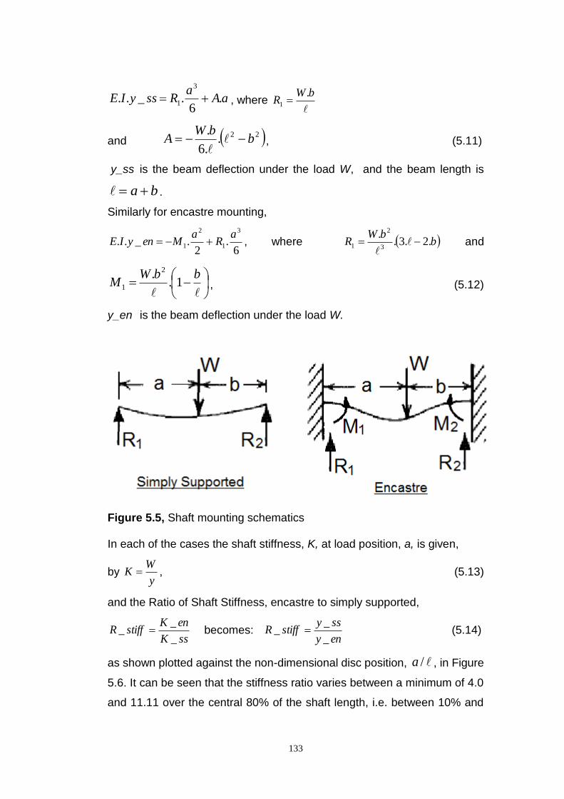
133
aAa
RssyIE .6
._..3
1 , where
bWR
.1
and 22..6
.b
bWA
, (5.11)
y_ss is the beam deflection under the load W, and the beam length is
ba .
Similarly for encastre mounting,
6.
2._..
3
1
2
1
aR
aMenyIE , where b
bWR .2.3.
.3
2
1
and
bbWM 1.
. 2
1 , (5.12)
y_en is the beam deflection under the load W.
Figure 5.5, Shaft mounting schematics In each of the cases the shaft stiffness, K, at load position, a, is given,
by y
WK , (5.13)
and the Ratio of Shaft Stiffness, encastre to simply supported,
ssK
enKstiffR
_
__ becomes:
eny
ssystiffR
_
__ (5.14)
as shown plotted against the non-dimensional disc position, /a , in Figure
5.6. It can be seen that the stiffness ratio varies between a minimum of 4.0
and 11.11 over the central 80% of the shaft length, i.e. between 10% and
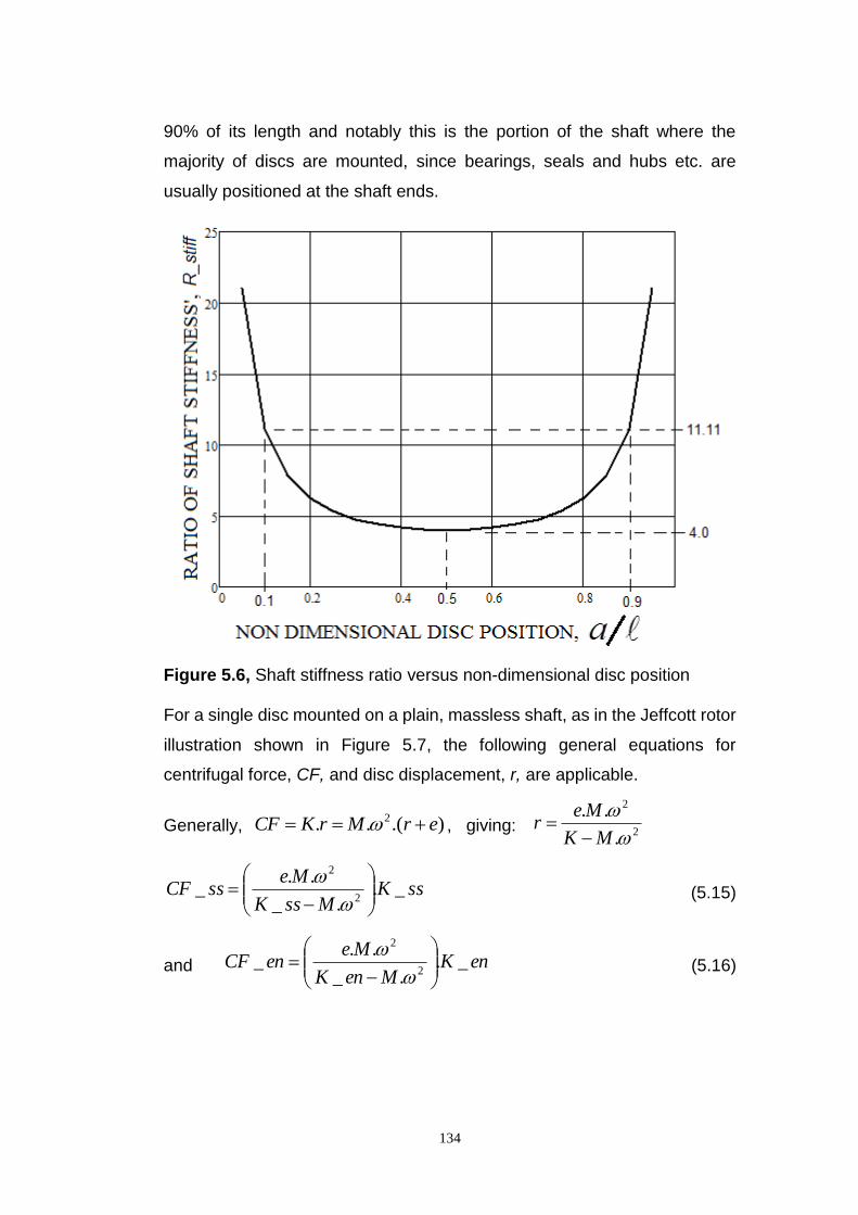
134
90% of its length and notably this is the portion of the shaft where the
majority of discs are mounted, since bearings, seals and hubs etc. are
usually positioned at the shaft ends.
Figure 5.6, Shaft stiffness ratio versus non-dimensional disc position For a single disc mounted on a plain, massless shaft, as in the Jeffcott rotor
illustration shown in Figure 5.7, the following general equations for
centrifugal force, CF, and disc displacement, r, are applicable.
Generally, ).(.. 2 erMrKCF , giving: 2
2
.
..
MK
Mer
ssKMssK
MessCF _.
._
.._
2
2
(5.15)
and enKMenK
MeenCF _.
._
.._
2
2
(5.16)
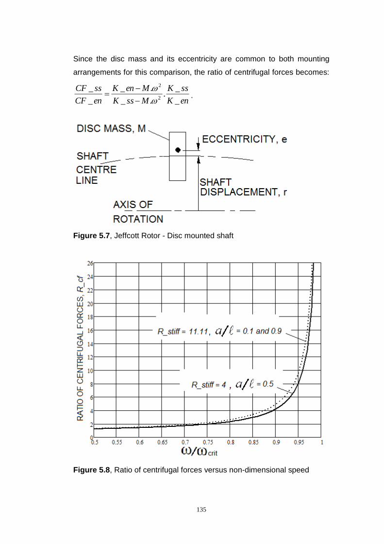
135
Since the disc mass and its eccentricity are common to both mounting
arrangements for this comparison, the ratio of centrifugal forces becomes:
enK
ssK
MssK
MenK
enCF
ssCF
_
_.
._
._
_
_2
2
.
Figure 5.7, Jeffcott Rotor - Disc mounted shaft
Figure 5.8, Ratio of centrifugal forces versus non-dimensional speed
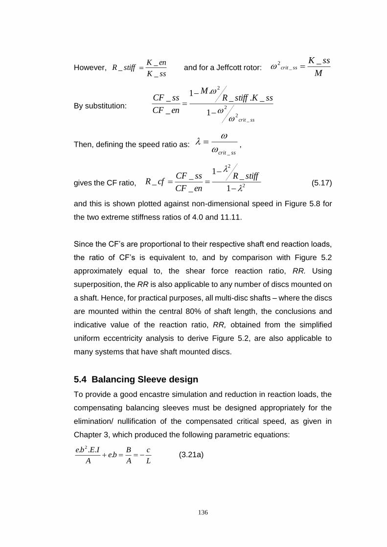
136
However, ssK
enKstiffR
_
__ and for a Jeffcott rotor:
M
ssKsscrit
__
2
By substitution:
sscrit
ssKstiffRM
enCF
ssCF
_2
2
2
1
_._.1
_
_
Then, defining the speed ratio as: sscrit _
,
gives the CF ratio, 2
2
1
_1
_
__
stiffR
enCF
ssCFcfR (5.17)
and this is shown plotted against non-dimensional speed in Figure 5.8 for
the two extreme stiffness ratios of 4.0 and 11.11.
Since the CF’s are proportional to their respective shaft end reaction loads,
the ratio of CF’s is equivalent to, and by comparison with Figure 5.2
approximately equal to, the shear force reaction ratio, RR. Using
superposition, the RR is also applicable to any number of discs mounted on
a shaft. Hence, for practical purposes, all multi-disc shafts – where the discs
are mounted within the central 80% of shaft length, the conclusions and
indicative value of the reaction ratio, RR, obtained from the simplified
uniform eccentricity analysis to derive Figure 5.2, are also applicable to
many systems that have shaft mounted discs.
5.4 Balancing Sleeve design
To provide a good encastre simulation and reduction in reaction loads, the
compensating balancing sleeves must be designed appropriately for the
elimination/ nullification of the compensated critical speed, as given in
Chapter 3, which produced the following parametric equations:
L
c
A
Bbe
A
IEbe .
... 2
(3.21a)
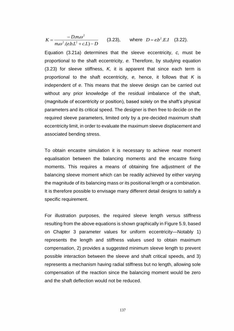
137
DLcLbem
mDK
)....(.
..22
2
(3.23), where IEbeD ... 2 (3.22).
Equation (3.21a) determines that the sleeve eccentricity, c, must be
proportional to the shaft eccentricity, e. Therefore, by studying equation
(3.23) for sleeve stiffness, K, it is apparent that since each term is
proportional to the shaft eccentricity, e, hence, it follows that K is
independent of e. This means that the sleeve design can be carried out
without any prior knowledge of the residual imbalance of the shaft,
(magnitude of eccentricity or position), based solely on the shaft’s physical
parameters and its critical speed. The designer is then free to decide on the
required sleeve parameters, limited only by a pre-decided maximum shaft
eccentricity limit, in order to evaluate the maximum sleeve displacement and
associated bending stress.
To obtain encastre simulation it is necessary to achieve near moment
equalisation between the balancing moments and the encastre fixing
moments. This requires a means of obtaining fine adjustment of the
balancing sleeve moment which can be readily achieved by either varying
the magnitude of its balancing mass or its positional length or a combination.
It is therefore possible to envisage many different detail designs to satisfy a
specific requirement.
For illustration purposes, the required sleeve length versus stiffness
resulting from the above equations is shown graphically in Figure 5.9, based
on Chapter 3 parameter values for uniform eccentricity—Notably 1)
represents the length and stiffness values used to obtain maximum
compensation, 2) provides a suggested minimum sleeve length to prevent
possible interaction between the sleeve and shaft critical speeds, and 3)
represents a mechanism having radial stiffness but no length, allowing sole
compensation of the reaction since the balancing moment would be zero
and the shaft deflection would not be reduced.
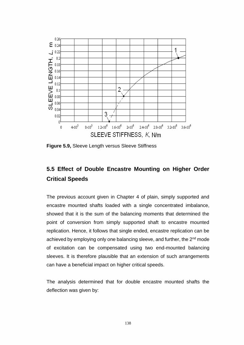
138
Figure 5.9, Sleeve Length versus Sleeve Stiffness
5.5 Effect of Double Encastre Mounting on Higher Order
Critical Speeds
The previous account given in Chapter 4 of plain, simply supported and
encastre mounted shafts loaded with a single concentrated imbalance,
showed that it is the sum of the balancing moments that determined the
point of conversion from simply supported shaft to encastre mounted
replication. Hence, it follows that single ended, encastre replication can be
achieved by employing only one balancing sleeve, and further, the 2nd mode
of excitation can be compensated using two end-mounted balancing
sleeves. It is therefore plausible that an extension of such arrangements
can have a beneficial impact on higher critical speeds.
The analysis determined that for double encastre mounted shafts the
deflection was given by:
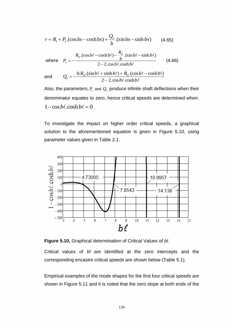
139
)sinh.(sin)cosh.(cos1 bxbxb
QbxbxPRr e
e (4.65)
where
bb
bbb
RbbR
P
ll
ecosh.cos.22
)sinh.(sin)cosh.(cos 11
(4.66)
and
bb
bbRbbRbQ ll
ecosh.cos.22
)cosh.(cos)sinh.(sin. 11
Also, the parameters, eP and eQ produce infinite shaft deflections when their
denominator equates to zero, hence critical speeds are determined when:
0cosh.cos1 bb .
To investigate the impact on higher order critical speeds, a graphical
solution to the aforementioned equation is given in Figure 5.10, using
parameter values given in Table 2.1.
Figure 5.10, Graphical determination of Critical Values of bl. Critical values of bl are identified at the zero intercepts and the
corresponding encastre critical speeds are shown below (Table 5.1).
Empirical examples of the mode shapes for the first four critical speeds are
shown in Figure 5.11 and it is noted that the zero slope at both ends of the
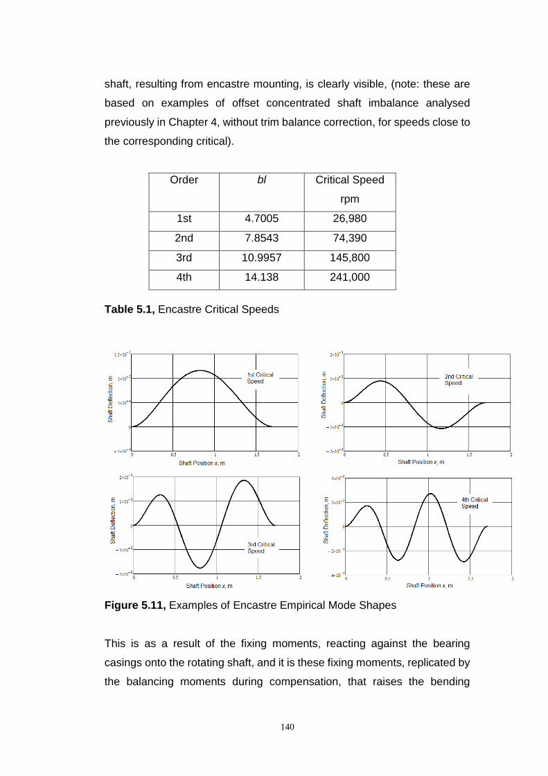
140
shaft, resulting from encastre mounting, is clearly visible, (note: these are
based on examples of offset concentrated shaft imbalance analysed
previously in Chapter 4, without trim balance correction, for speeds close to
the corresponding critical).
Order bl Critical Speed
rpm
1st 4.7005 26,980
2nd 7.8543 74,390
3rd 10.9957 145,800
4th 14.138 241,000
Table 5.1, Encastre Critical Speeds
Figure 5.11, Examples of Encastre Empirical Mode Shapes This is as a result of the fixing moments, reacting against the bearing
casings onto the rotating shaft, and it is these fixing moments, replicated by
the balancing moments during compensation, that raises the bending

141
stiffness of the shaft and thereby increases its critical speeds, above those
of an equivalent, simply supported shaft.
5.6 Simulation Ratio
For comparison purposes, previous analysis of equivalent simply supported
shafts, chapter 2, section 2.4, based on Table 2.1 parameter values,
produced the following critical speeds, shown in Table 5.2.
Noting that for a simple spring-mass system, stiffness is proportional to
natural frequency squared, then by defining:
Simulation Ratio, 𝑆𝑅 = (𝐸𝑛𝑐𝑎𝑠𝑡𝑟𝑒 𝐶𝑟𝑖𝑡 𝑆𝑝𝑒𝑒𝑑
𝑆.𝑆.𝐶𝑟𝑖𝑡 𝑆𝑝𝑒𝑒𝑑)
2.
It can be seen that this ratio, as shown in Table 5.3, reduces as the critical
speed increases, since each additional undulation of the mode shape
reduces the influence of the fixing moments, i.e. it is only the end
undulations that are effectively single encastre mounted, whereas the
remaining undulations are simply supported, since they are not restrained
by fixing moments.
Order bl Critical Speed
rpm
1st π 11,900
2nd 2π 47,610
3rd 3π 107,100
4th 4π 190,400
Table 5.2, Simply Supported Critical Speeds
Therefore, the SR ratio gives an indication of the overall stiffening effect of
the fixing moments on a full shaft assembly and by analogy the possible
benefits to be gained by encastre simulation, provided the balancing sleeve
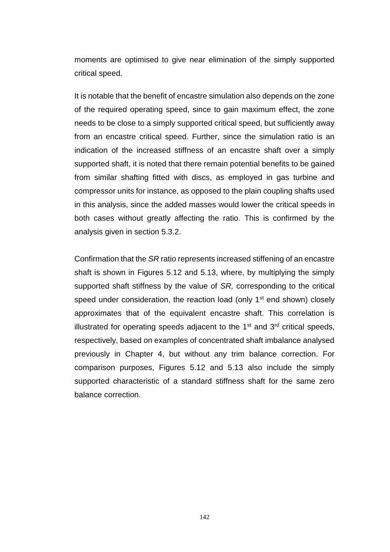
142
moments are optimised to give near elimination of the simply supported
critical speed.
It is notable that the benefit of encastre simulation also depends on the zone
of the required operating speed, since to gain maximum effect, the zone
needs to be close to a simply supported critical speed, but sufficiently away
from an encastre critical speed. Further, since the simulation ratio is an
indication of the increased stiffness of an encastre shaft over a simply
supported shaft, it is noted that there remain potential benefits to be gained
from similar shafting fitted with discs, as employed in gas turbine and
compressor units for instance, as opposed to the plain coupling shafts used
in this analysis, since the added masses would lower the critical speeds in
both cases without greatly affecting the ratio. This is confirmed by the
analysis given in section 5.3.2.
Confirmation that the SR ratio represents increased stiffening of an encastre
shaft is shown in Figures 5.12 and 5.13, where, by multiplying the simply
supported shaft stiffness by the value of SR, corresponding to the critical
speed under consideration, the reaction load (only 1st end shown) closely
approximates that of the equivalent encastre shaft. This correlation is
illustrated for operating speeds adjacent to the 1st and 3rd critical speeds,
respectively, based on examples of concentrated shaft imbalance analysed
previously in Chapter 4, but without any trim balance correction. For
comparison purposes, Figures 5.12 and 5.13 also include the simply
supported characteristic of a standard stiffness shaft for the same zero
balance correction.
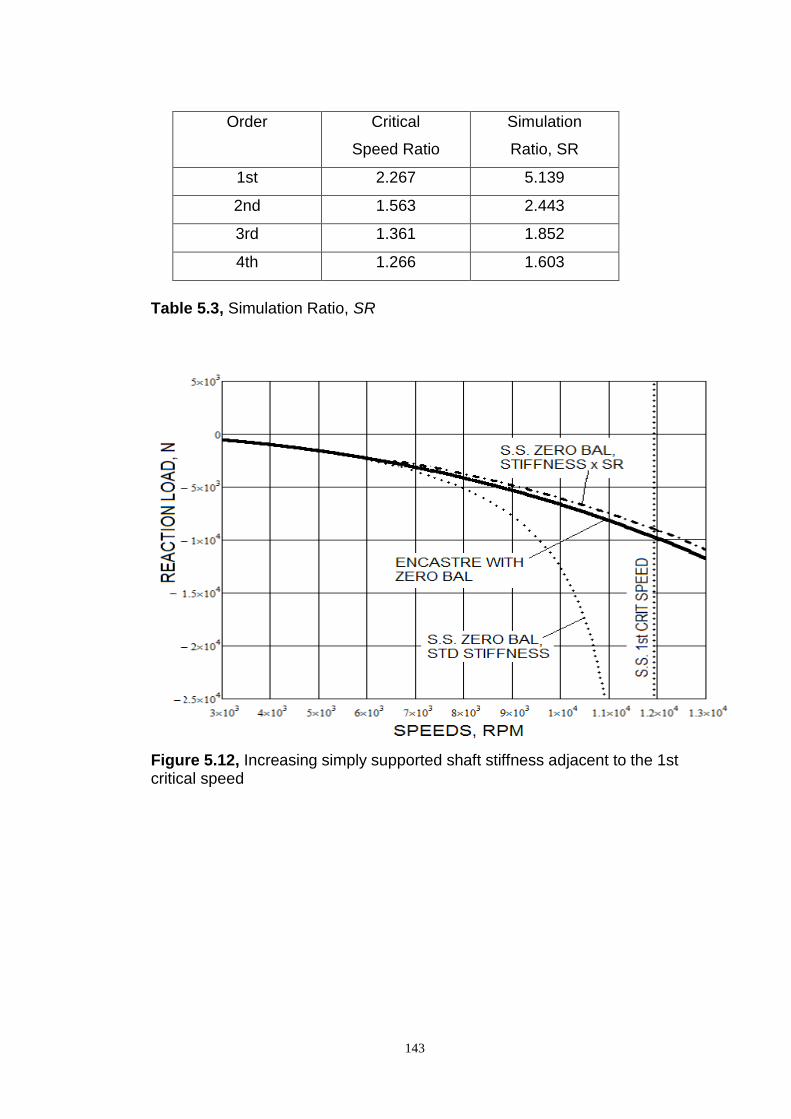
143
Order Critical
Speed Ratio
Simulation
Ratio, SR
1st 2.267 5.139
2nd 1.563 2.443
3rd 1.361 1.852
4th 1.266 1.603
Table 5.3, Simulation Ratio, SR
Figure 5.12, Increasing simply supported shaft stiffness adjacent to the 1st critical speed

144
Figure 5.13, Increasing simply supported shaft stiffness adjacent to the 3rd critical speed Study of the simply supported equations, chapter 4, section 4.3, determined
that the requirements for elimination of the 1st classical critical speed and by
substitution of the values of bl corresponding to the higher order critical
speeds, ( 2b , 3 , 4 etc.), that the same controlling condition applies
for these critical speeds, i.e.
IEbkeMM ..2.. 2
0201 , equation (4.64).
Also, when the same values of bl are applied to the sum of the encastre
fixing moments to represent encastre operation at simply supported critical
speeds, the requirement is also unchanged, i.e.
IEbkeMM ff ..2.. 2
21 , equation (4.69).
This identity is the same as that derived for the 1st classical critical speed in
Chapter 3, and the resulting equalisation of the balancing and fixing
moments shows that encastre conversion is also present at these higher
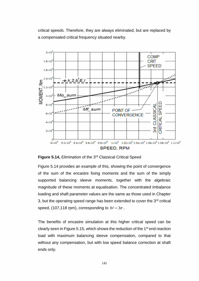
145
critical speeds. Therefore, they are always eliminated, but are replaced by
a compensated critical frequency situated nearby.
Figure 5.14, Elimination of the 3rd Classical Critical Speed Figure 5.14 provides an example of this, showing the point of convergence
of the sum of the encastre fixing moments and the sum of the simply
supported balancing sleeve moments, together with the algebraic
magnitude of these moments at equalisation. The concentrated imbalance
loading and shaft parameter values are the same as those used in Chapter
3, but the operating speed range has been extended to cover the 3rd critical
speed, (107,118 rpm), corresponding to 3b .
The benefits of encastre simulation at this higher critical speed can be
clearly seen in Figure 5.15, which shows the reduction of the 1st end reaction
load with maximum balancing sleeve compensation, compared to that
without any compensation, but with low speed balance correction at shaft
ends only.
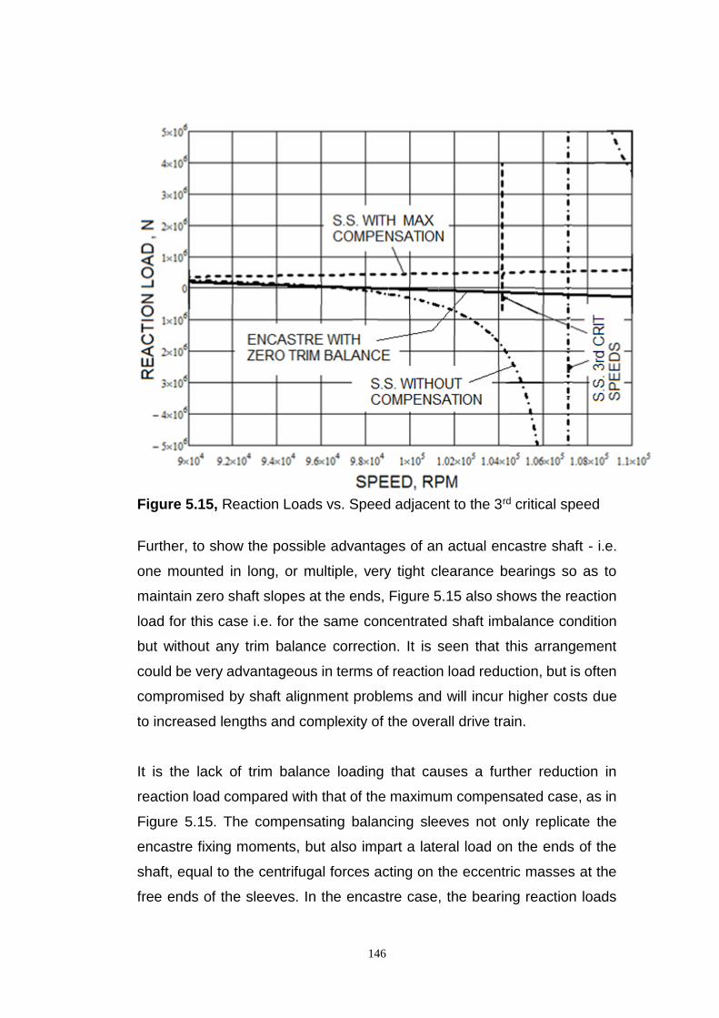
146
Figure 5.15, Reaction Loads vs. Speed adjacent to the 3rd critical speed
Further, to show the possible advantages of an actual encastre shaft - i.e.
one mounted in long, or multiple, very tight clearance bearings so as to
maintain zero shaft slopes at the ends, Figure 5.15 also shows the reaction
load for this case i.e. for the same concentrated shaft imbalance condition
but without any trim balance correction. It is seen that this arrangement
could be very advantageous in terms of reaction load reduction, but is often
compromised by shaft alignment problems and will incur higher costs due
to increased lengths and complexity of the overall drive train.
It is the lack of trim balance loading that causes a further reduction in
reaction load compared with that of the maximum compensated case, as in
Figure 5.15. The compensating balancing sleeves not only replicate the
encastre fixing moments, but also impart a lateral load on the ends of the
shaft, equal to the centrifugal forces acting on the eccentric masses at the
free ends of the sleeves. In the encastre case, the bearing reaction loads
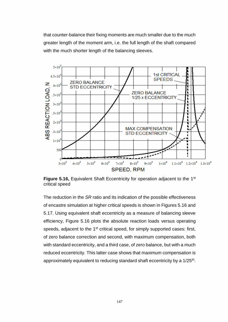
147
that counter-balance their fixing moments are much smaller due to the much
greater length of the moment arm, i.e. the full length of the shaft compared
with the much shorter length of the balancing sleeves.
Figure 5.16, Equivalent Shaft Eccentricity for operation adjacent to the 1st critical speed
The reduction in the SR ratio and its indication of the possible effectiveness
of encastre simulation at higher critical speeds is shown in Figures 5.16 and
5.17. Using equivalent shaft eccentricity as a measure of balancing sleeve
efficiency, Figure 5.16 plots the absolute reaction loads versus operating
speeds, adjacent to the 1st critical speed, for simply supported cases: first,
of zero balance correction and second, with maximum compensation, both
with standard eccentricity, and a third case, of zero balance, but with a much
reduced eccentricity. This latter case shows that maximum compensation is
approximately equivalent to reducing standard shaft eccentricity by a 1/25th.
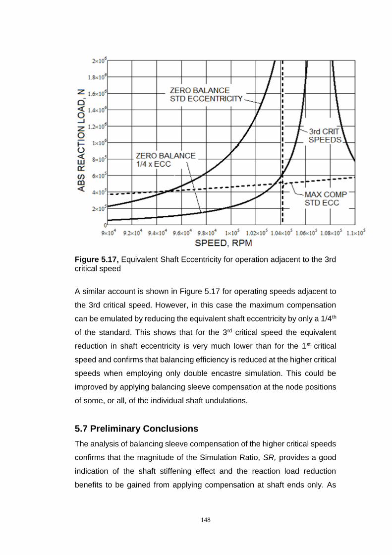
148
Figure 5.17, Equivalent Shaft Eccentricity for operation adjacent to the 3rd critical speed
A similar account is shown in Figure 5.17 for operating speeds adjacent to
the 3rd critical speed. However, in this case the maximum compensation
can be emulated by reducing the equivalent shaft eccentricity by only a 1/4th
of the standard. This shows that for the 3rd critical speed the equivalent
reduction in shaft eccentricity is very much lower than for the 1st critical
speed and confirms that balancing efficiency is reduced at the higher critical
speeds when employing only double encastre simulation. This could be
improved by applying balancing sleeve compensation at the node positions
of some, or all, of the individual shaft undulations.
5.7 Preliminary Conclusions
The analysis of balancing sleeve compensation of the higher critical speeds
confirms that the magnitude of the Simulation Ratio, SR, provides a good
indication of the shaft stiffening effect and the reaction load reduction
benefits to be gained from applying compensation at shaft ends only. As
149
expected, this ratio and its associated benefits are reduced as the order of
the critical speed increases since it is only the end undulations that are
subjected to single encastre simulation, and remaining undulations act as if
simply supported. However, notably, the analysis also confirms that
encastre simulation is still possible at higher critical speeds providing the
same mathematical requirements, (as for the 1st critical speed) are met, i.e.
the sum of the balancing moments equals the sum of the encastre fixing
moments, IEbkeMMMM ff ..2.. 2
210201 .
It is also noted that due to the very high rotational speeds, even with
maximum balance sleeve compensation, the reaction loads are an order of
magnitude higher than when operating near the 1st critical speed. Hence the
importance of achieving the lowest possible degree of residual imbalance
for high speed machinery remains paramount. However, design of very high
speed machinery remains a compromise between cost and layout
possibilities, for example: 1) by minimising eccentricity, through maintaining
material stability by close control of density, grain structure and internal
properties such as creep and hysteresis; together with ultra-high precision
machining of multi component assemblies or alternatively, by production of
one piece rotors, 2) by maintaining large, lateral critical speed, LCS,
margins, i.e. ensuring that the critical speed is well away from the running
speed; this is usually a conflicting requirement needing rotating components
to be of both of high lateral stiffness and of low mass. Alternately, LCS
margins may be increased by the use of additional bearings, at shaft ends
and/ or mid span, as per actual encastre mounting. However, all these
possibilities invariably add to the overall complexity of the design layout with
associated issues. Hence, achieving and maintaining (often during very
arduous operating conditions) a very low degree of residual unbalance is
not easy, and consequently installations often suffer from severe vibration
problems at particular speeds and/ or loading conditions.
150
Therefore, even at the higher critical speeds, with its reduced benefits, the
possibility of near elimination/ nullification of an adjacent critical speed as
offered by shaft-end balance compensation, still has the potential to help
reduce shaft vibrations. And, it is noted that overall shaft balance could be
improved even further, if required, by applying balancing sleeve
compensation at node positions along the shaft so as to replicate encastre
mounting of some, or all, of the intermediate shaft undulations.
The analysis of the shear force reaction ratio, RR, has showed that it can
be considered independent of the shaft eccentricity, and provides an
indication of the possible benefits to be gained by encastre simulation for
any given level of shaft eccentricity. This means that even if a shaft has
been previously balanced by a maximum practical amount, for example on
a high speed balancing machine, then this methodology has the effect of
further reducing the eccentricity by RR (noting that the internal shear
reaction force is directly proportional to shaft eccentricity), even allowing for
the fact that the exact value of the ratio applies only at the speed at which
encastre conversion occurs, i.e. when the balancing sleeve moments
equate to the encastre fixing moments. Moreover, since the ratio greatly
increases the closer the operating speed is to the critical speed, then it
follows that the balancing improvements also increase to counter the usual
increase in rotor vibration that occurs at these higher speeds – an ideal
situation.
The example case of maximum compensation of the 1st critical speed,
shown in Figure 5.16, produced an equivalent reduction in shaft eccentricity
that was greater than 25x. If utilised it would be extremely advantageous to
many industrial machines, by imparting improved system performance, if
allowed to operate with reduced lateral critical speed margins.
The analysis implies that this is also feasible for most designs of high-speed
flexible shafts. Although the analysis is based on a simple plain shaft with
151
uniform eccentricity, it is shown that the benefits also apply to shafts with
concentrated imbalances and/or multiple discs that are mounted within the
central 80% of the shaft length, i.e. most practical shafting. Also, it is shown
that the characteristic design of the balancing sleeves to achieve maximum
balance compensation is independent of shaft eccentricity. Therefore, prior
knowledge of the residual imbalance of the shaft (magnitude of eccentricity
or position) is not needed and fine adjustment of the balancing sleeve
moment to give encastre simulation should be possible by a variety of
detailed designs, capable of achieving near micrometer accuracy, in
response to feedback data from the bearing sensors (a pre-requisite in most
large industrial high-speed drive trains).
The significant potential of this novel balancing methodology to provide
improvements in the balancing of high-speed, flexible shafts, has therefore
been shown.

152
Chapter 6
6.1 Test Rig Design
The production of a full size test shaft that replicates the drive couplings
employed by Siemens sub 15MW turbine packages is prohibitively
expensive, both in terms of capital and commission costs, and
infrastructure. However, validation of balance sleeve compensation theory
and its practical potential can be met using a scaled test rig facility designed
to have full speed capability. The speed matching maintains parity between
site and test critical speeds, and is sized to accommodate a reduced scaled
model example of a turbine coupling shaft. The test facility is described
below.
Figure 6.1, Test Rig
153
The drive system is comprised of two Oswald, Type QDi13 2 2, variable
speed, 0 – 20,000 rpm, 49 kW, electric motors, LHS driving, RHS acting as
a feedback generator, so that only the accelerating torque and drive train
losses needed to be powered electrically by the mains supply. The motors
and its control package is designed and supplied by Control Techniques
Ltd., as specified in Appendix D1.
The motors are mounted on individual bed plates, via a pair of slide rails, to
allow lengthwise adjustment of a test shaft, which is centrally mounted
between the shaft ends, as shown in Figure 6.1.
6.2 Instrumentation
Instrumentation is used to measure the balance condition of the test shaft
under a known level of shaft imbalance at a variety of steady state speeds—
initially without any trim balance correction and then with a series of
balancing sleeve compensations. A non-contacting system of measurement
is used so as to avoid affecting the vibration measurements—laser based
systems are capable of measuring deflection of high speed rotating
elements and therefore adequately meet this requirement. Optical
triangulation is used to determine deflection.
Instrumentation consists of 3x Micro-Epsilon, free standing lasers systems
(optoNCDT, type ILD 2300-20), as specified in Appendix D2, positioned to
separately enable deflection measurements of the LHS sleeve, the shaft
mid-point and the RHS sleeve, as a result of their respective unbalance
during shaft rotation.
Markers are bonded at the top dead centre (TDC) position on the outside
diameter of each laser location to provide a consistent key phaser/trigger
point during each rotation of the shaft. This allowed vector formulation of
peak—to–peak, deflections and angular offsets between the local heavy

154
spot of section unbalance and the shaft TDC position. Hence, at each test
speed it is possible to translate local deflections onto the plane of unbalance
produced by a known level of added shaft unbalance, thereby allowing a
direct comparisons to be made with theoretical results, for validation
purposes.
6.3 Test Coupling Shaft
With reference to balancing problems seen by some Siemens sub 15MW
turbine applications and the site equivalent analytical models developed in
Chapters 2 and 3, the application of Buckingham’s Pi theorem, of non-
dimensional analysis, determined that a suitably scaled test shaft could be
produced provided parity was maintained between the two critical speeds.
Whilst complying with this requirement, a test shaft was designed in
conjunction with Bibby Turboflex Transmissions Ltd., details of which are
given in Table 6.1. A laminated, disc type, flexible element assembly pack,
from their standard Torsiflex range of couplings is used. This is a 6 bolt
design of similar construction to couplings typically used for mechanical
drive contracts and their minimum size, code number TF27, is found to be
an appropriate match with the size requirements of the spacer tube, as
specified in Appendix D3. The spacer tube is a plain tubular component
fitted between the flexible element assembly packs.
For validation purposes it is necessary to apply imbalance masses to the
spacer tube to replicate a point of concentrated unbalance, as in the
analysis given in Chapter 4. It is also recognised that any method of
imbalance attachment must have a minimum effect on the tube’s bending
stiffness and mass so as to avoid changes to its critical speed. This is
achieved by the addition of 5 narrow, low profile, dovetail rings, positioned
at the mid point of 5 zones, of approximately equal length, set out axially
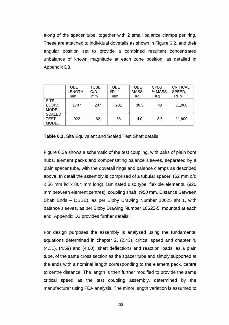
155
along of the spacer tube, together with 2 small balance clamps per ring.
These are attached to individual dovetails as shown in Figure 6.2, and their
angular position set to provide a combined resultant concentrated
unbalance of known magnitude at each zone position, as detailed in
Appendix D3.
TUBE LENGTH, mm
TUBE O/D, mm
TUBE I/D, mm
TUBE MASS, Kg
CPLG ½ MASS, Kg
CRITICAL SPEED, RPM
SITE EQUIV. MODEL
1707
207
201
38.3
48
11,900
SCALED TEST MODEL
922
62
56
4.0
3.6
11,900
Table 6.1, Site Equivalent and Scaled Test Shaft details
Figure 6.3a shows a schematic of the test coupling, with pairs of plain bore
hubs, element packs and compensating balance sleeves, separated by a
plain spacer tube, with the dovetail rings and balance clamps as described
above. In detail the assembly is comprised of a tubular spacer, (62 mm o/d
x 56 mm i/d x 864 mm long), laminated disc type, flexible elements, (920
mm between element centres), coupling shaft, (950 mm, Distance Between
Shaft Ends – DBSE), as per Bibby Drawing Number 10625 sht 1, with
balance sleeves, as per Bibby Drawing Number 10625-5, mounted at each
end. Appendix D3 provides further details.
For design purposes the assembly is analysed using the fundamental
equations determined in chapter 2, (2.43), critical speed and chapter 4,
(4.31), (4.59) and (4.60), shaft deflections and reaction loads, as a plain
tube, of the same cross section as the spacer tube and simply supported at
the ends with a nominal length corresponding to the element pack, centre
to centre distance. The length is then further modified to provide the same
critical speed as the test coupling assembly, determined by the
manufacturer using FEA analysis. The minor length variation is assumed to
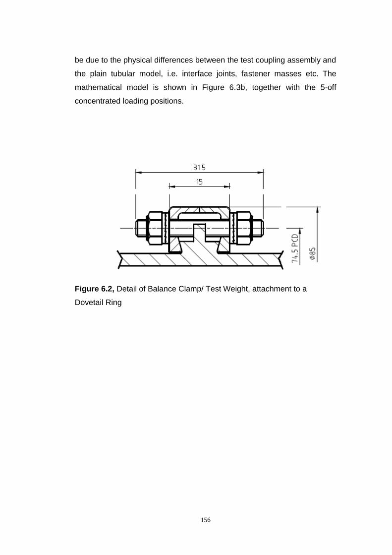
156
be due to the physical differences between the test coupling assembly and
the plain tubular model, i.e. interface joints, fastener masses etc. The
mathematical model is shown in Figure 6.3b, together with the 5-off
concentrated loading positions.
Figure 6.2, Detail of Balance Clamp/ Test Weight, attachment to a
Dovetail Ring

157
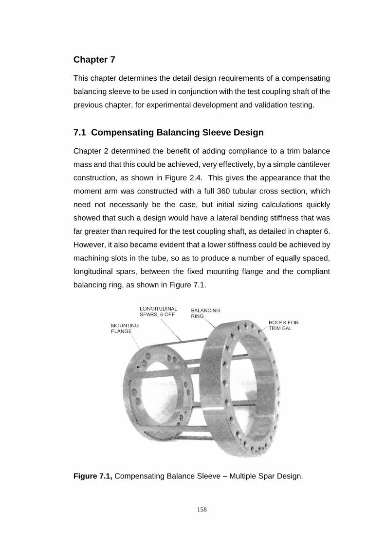
158
Chapter 7 This chapter determines the detail design requirements of a compensating
balancing sleeve to be used in conjunction with the test coupling shaft of the
previous chapter, for experimental development and validation testing.
7.1 Compensating Balancing Sleeve Design Chapter 2 determined the benefit of adding compliance to a trim balance
mass and that this could be achieved, very effectively, by a simple cantilever
construction, as shown in Figure 2.4. This gives the appearance that the
moment arm was constructed with a full 360 tubular cross section, which
need not necessarily be the case, but initial sizing calculations quickly
showed that such a design would have a lateral bending stiffness that was
far greater than required for the test coupling shaft, as detailed in chapter 6.
However, it also became evident that a lower stiffness could be achieved by
machining slots in the tube, so as to produce a number of equally spaced,
longitudinal spars, between the fixed mounting flange and the compliant
balancing ring, as shown in Figure 7.1.
Figure 7.1, Compensating Balance Sleeve – Multiple Spar Design.
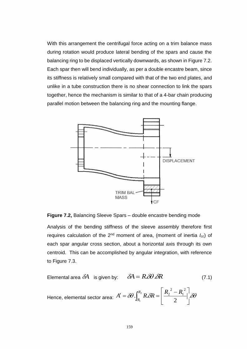
159
With this arrangement the centrifugal force acting on a trim balance mass
during rotation would produce lateral bending of the spars and cause the
balancing ring to be displaced vertically downwards, as shown in Figure 7.2.
Each spar then will bend individually, as per a double encastre beam, since
its stiffness is relatively small compared with that of the two end plates, and
unlike in a tube construction there is no shear connection to link the spars
together, hence the mechanism is similar to that of a 4-bar chain producing
parallel motion between the balancing ring and the mounting flange.
Figure 7.2, Balancing Sleeve Spars – double encastre bending mode Analysis of the bending stiffness of the sleeve assembly therefore first
requires calculation of the 2nd moment of area, (moment of inertia Icc) of
each spar angular cross section, about a horizontal axis through its own
centroid. This can be accomplished by angular integration, with reference
to Figure 7.3.
Elemental area A is given by: RRA .. (7.1)
Hence, elemental sector area: .2
..2
1
2
1
2
2
R
R
RRRRA

160
Spar cross sectional area: ).(2
. 12
2
1
2
22
1
RRAA (7.2)
Figure 7.3, Single Spar Cross Sectional Analysis. The 1st moment of area about axis X – X, of the spar cross section, A, is given by:
2
1
2
1
.sin.1
ARM
R
R, and substituting from (7.1) gives:
2
1
2
1
.sin..2
1
R
RRRM , and integrating wrt R gives:
2
1
.sin.3
3
1
3
21
RRM , and integrating wrt θ gives:
21
3
1
3
21 coscos.
3
RRM , (7.3)
Therefore, the centroid height of the spar cross section, above axis X – X, is given by:
161
A
Mh 1 , (7.4)
and is readily obtainable from (7.3) and (7.2). Similarly, the 2nd moment of area about axis X – X, (moment of inertia, Ixx) of the spar cross section, A, is given by:
2
1
2
1
.sin.2
2
ARM
R
R, and substituting from (7.1) gives:
.sin.....sin. 232
2
2
1
2
1
2
1
2
1
RRRRRM
R
R
R
R
2
1
.sin.4
2
4
1
4
22
RRM
Substituting, 2
2cos1sin2
, and integrating gives:
4
2sin
24
2sin
2.
4
1122
4
1
4
22
RRM , (7.5)
The 2nd moment of area, or moment of inertia, through the centroid can now be determined from the parallel axis theorem:
2.hAII ccxx
Hence, the moment of inertia for an individual spar is given by:
2
2 .hAMIcc (7.6)
Since each spar will experience the same deflection, the individual bending
stiffness’ are deemed to act in parallel and the overall stiffness, of the
complete assembly, will be the summation of all the individual stiffness’.
Also, beam theory states that for elastic deflection, the stiffness of a beam
is directly proportional to its moment of inertia, so it follows that the sleeve
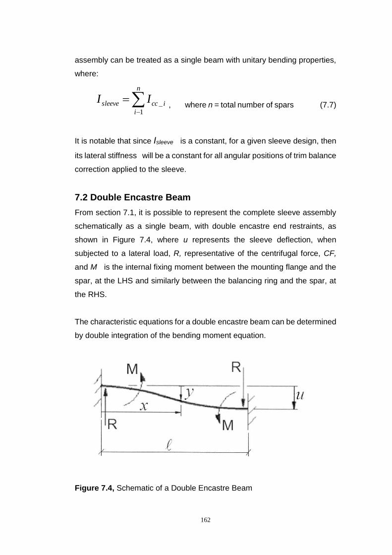
162
assembly can be treated as a single beam with unitary bending properties,
where:
n
i
iccsleeve II1
_ , where n = total number of spars (7.7)
It is notable that since Isleeve is a constant, for a given sleeve design, then
its lateral stiffness will be a constant for all angular positions of trim balance
correction applied to the sleeve.
7.2 Double Encastre Beam
From section 7.1, it is possible to represent the complete sleeve assembly
schematically as a single beam, with double encastre end restraints, as
shown in Figure 7.4, where u represents the sleeve deflection, when
subjected to a lateral load, R, representative of the centrifugal force, CF,
and M is the internal fixing moment between the mounting flange and the
spar, at the LHS and similarly between the balancing ring and the spar, at
the RHS.
The characteristic equations for a double encastre beam can be determined
by double integration of the bending moment equation.
Figure 7.4, Schematic of a Double Encastre Beam
163
From beam theory, the bending moment, BM, is equal to:
xRMdx
ydIEBM ...
2
2
, (7.8)
By integration, AxR
xMdx
dyIE
2
....
2
BxAxRxM
yIE .6
.
2
...
32
where A and B are constants of integration and both are equal to zero, since
at 0x , 0y and 0dx
dy, therefore:
6
.
2
...
32 xRxMyIE , (7.9)
The LHS of (7.8) and (7.9) equal M and -EI.u, respectively for x giving:
2
.RM , (7.10)
and by substitution 12
...
3RuIE , (7.11)
Combining (7.10) and (7.11) gives 2
..6
EIuM , (7.12)
The beam/ sleeve stiffness is then given by 3
.12
EI
u
RK , (7.13)
The maximum bending stress in any given spar appears at shaft ends
resulting from the imposed fixing moments, and is given by:
fibreyI
Mf .max_ ,
where fibrey is the extreme fibre, seen during bending, i.e. the vertical
height of the outmost point on the spar cross section above the centroid
position.
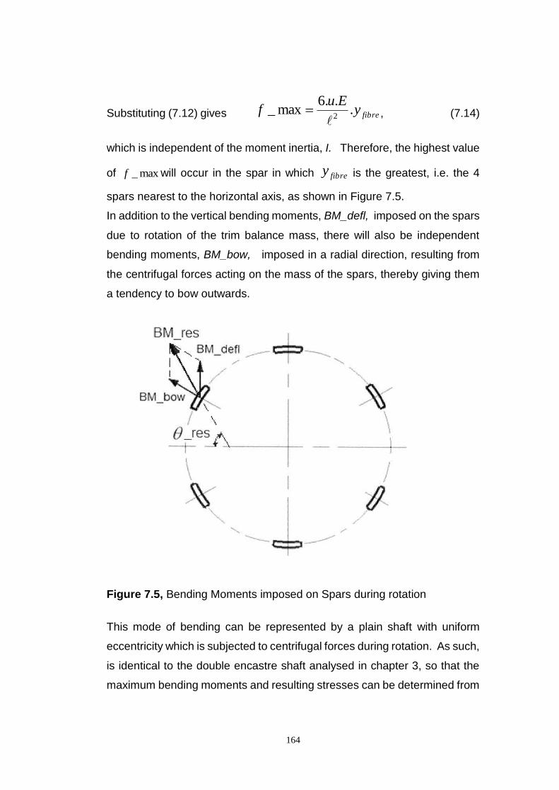
164
Substituting (7.12) gives fibreyEu
f ...6
max_2
, (7.14)
which is independent of the moment inertia, I. Therefore, the highest value
of max_f will occur in the spar in which fibrey is the greatest, i.e. the 4
spars nearest to the horizontal axis, as shown in Figure 7.5.
In addition to the vertical bending moments, BM_defl, imposed on the spars
due to rotation of the trim balance mass, there will also be independent
bending moments, BM_bow, imposed in a radial direction, resulting from
the centrifugal forces acting on the mass of the spars, thereby giving them
a tendency to bow outwards.
Figure 7.5, Bending Moments imposed on Spars during rotation
This mode of bending can be represented by a plain shaft with uniform
eccentricity which is subjected to centrifugal forces during rotation. As such,
is identical to the double encastre shaft analysed in chapter 3, so that the
maximum bending moments and resulting stresses can be determined from
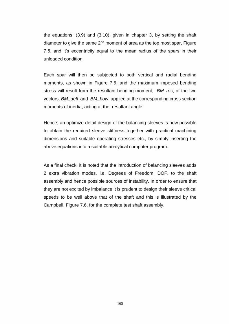
165
the equations, (3.9) and (3.10), given in chapter 3, by setting the shaft
diameter to give the same 2nd moment of area as the top most spar, Figure
7.5, and it’s eccentricity equal to the mean radius of the spars in their
unloaded condition.
Each spar will then be subjected to both vertical and radial bending
moments, as shown in Figure 7.5, and the maximum imposed bending
stress will result from the resultant bending moment, BM_res, of the two
vectors, BM_defl and BM_bow, applied at the corresponding cross section
moments of inertia, acting at the resultant angle,
Hence, an optimize detail design of the balancing sleeves is now possible
to obtain the required sleeve stiffness together with practical machining
dimensions and suitable operating stresses etc., by simply inserting the
above equations into a suitable analytical computer program.
As a final check, it is noted that the introduction of balancing sleeves adds
2 extra vibration modes, i.e. Degrees of Freedom, DOF, to the shaft
assembly and hence possible sources of instability. In order to ensure that
they are not excited by imbalance it is prudent to design their sleeve critical
speeds to be well above that of the shaft and this is illustrated by the
Campbell, Figure 7.6, for the complete test shaft assembly.

166
Figure 7.6, Campbell Diagram of Test Shaft

167
Chapter 8
8.1 Test Requirements
Following the establishment of balance sleeve compensation and its
associated encastre simulation theory, Chapters 2, 3 and 4, the results
require practical validation. An instrumented test rig and scaled coupling
test shaft has therefore been designed and commissioned, as described in
Chapter 6.
Experimental trials are conducted in accordance with the following
procedures.
8.2 Test Procedure
SAFETY PRECAUTIONS APPLICABLE TO ALL TESTS
To prevent failure of the coupling shaft assembly, operation close to the
critical speed is limited by laser monitoring and manual shutdown if safe
shaft and sleeve deflections are reached/exceeded.
Safe Limits are set at shaft mid-point and sleeve balance ring deflections
of 6.0 mm and 0.35 mm, respectively, (corresponding stresses; 65% and
70% of yield).
Measurements to be taken at steady state operating speeds with step
changes gradually reduced as deflection readings increase, to maintain
shaft and sleeve deflections below stated safe limits. Chart 1 is to be used
as a guide to likely increases in shaft dynamic magnification of deflections
in the zero balance correction condition, with shaft critical speed proximity.
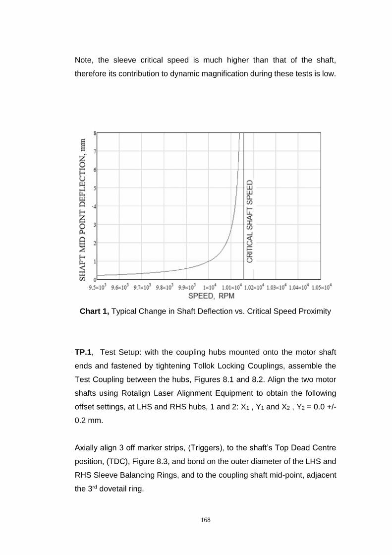
168
Note, the sleeve critical speed is much higher than that of the shaft,
therefore its contribution to dynamic magnification during these tests is low.
Chart 1, Typical Change in Shaft Deflection vs. Critical Speed Proximity
TP.1, Test Setup: with the coupling hubs mounted onto the motor shaft
ends and fastened by tightening Tollok Locking Couplings, assemble the
Test Coupling between the hubs, Figures 8.1 and 8.2. Align the two motor
shafts using Rotalign Laser Alignment Equipment to obtain the following
offset settings, at LHS and RHS hubs, 1 and 2: X1 , Y1 and X2 , Y2 = 0.0 +/-
0.2 mm.
Axially align 3 off marker strips, (Triggers), to the shaft’s Top Dead Centre
position, (TDC), Figure 8.3, and bond on the outer diameter of the LHS and
RHS Sleeve Balancing Rings, and to the coupling shaft mid-point, adjacent
the 3rd dovetail ring.
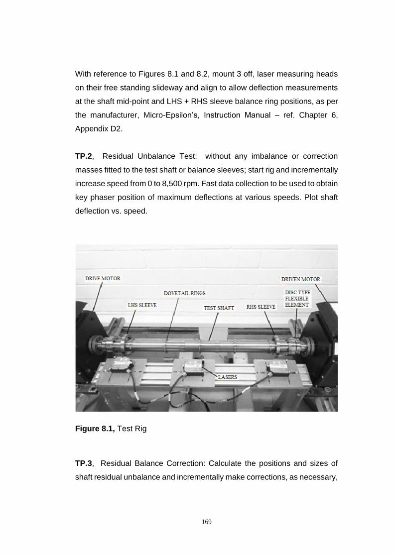
169
With reference to Figures 8.1 and 8.2, mount 3 off, laser measuring heads
on their free standing slideway and align to allow deflection measurements
at the shaft mid-point and LHS + RHS sleeve balance ring positions, as per
the manufacturer, Micro-Epsilon’s, Instruction Manual – ref. Chapter 6,
Appendix D2.
TP.2, Residual Unbalance Test: without any imbalance or correction
masses fitted to the test shaft or balance sleeves; start rig and incrementally
increase speed from 0 to 8,500 rpm. Fast data collection to be used to obtain
key phaser position of maximum deflections at various speeds. Plot shaft
deflection vs. speed.
Figure 8.1, Test Rig
TP.3, Residual Balance Correction: Calculate the positions and sizes of
shaft residual unbalance and incrementally make corrections, as necessary,

170
by adding or removing metal from the sleeves and the two central balancing
rings on the shaft, and re-check test TP.2.
Repeat as necessary to achieve repeatable low levels of shaft deflections,
(less than 0.5 mm), at speeds up to 10,200 rpm. Plot ‘Residual’ shaft
deflection vs speed.
Figure 8.2, Close-Up of Test Weights & LHS Laser Configuration
TP.4, Shaft Test Weight Unbalance with Zero Correction - without
Compensation: affix balance clamps to give 67.5 g.mm of imbalance, (2
clamps fitted to 2nd dovetail ring, 9º from diametric opposite position,
arranged as per Figure 8.3). Start rig and incrementally increase speed from
0 to 8,500 rpm. Fast data collection to be used to obtain key phaser position
of maximum deflection at various speeds. Plot ‘Measured’ shaft and sleeve
deflection vs. speed.
171
Check results and if deflections are well within stated limits, repeat test at
up to 10,000 rpm.
Figure 8.3, Angular relationship of Test Weights and Trigger (TDC)
position
TP.5, Double Sleeve Compensation Test: repeat step TP.4, with 68 gmm,
(1.3 gram at 51 mm radius) of balance sleeve compensation, 180 degrees
out of phase with shaft imbalance centrifugal force, CF, Figure 8.3, at both
balance sleeves. Plot ‘Measured’ shaft and sleeve deflection vs. speed.
TP.6, Analyse results and incrementally make further balance adjustments/
re-tests as appropriate to achieve maximum obtainable balance
compensation.
172
TP.7 Single Sleeve Compensation Test, LHS: repeat steps TP.5 and TP.6,
with 136 gmm, (2.6 gram at 51 mm radius), of balance sleeve
compensation, 180 degrees out of phase with shaft imbalance, at LHS
balance sleeve only – zero compensation at RHS sleeve. Plot ‘Measured’
shaft and sleeve deflection vs. speed.
TP.8, Analyse results and incrementally make further balance adjustments/
re-tests as appropriate to achieve maximum obtainable balance
compensation.
TP.9 Single Sleeve Compensation Test, RHS: repeat steps TP.5 and TP.6,
with 136 gmm, (2.6 gram at 51 mm radius) of balance sleeve compensation,
180 degrees out of phase with shaft imbalance, at RHS balance sleeve only
– zero compensation at LHS sleeve. Plot ‘Measured’ shaft and sleeve
deflection vs. speed.
TP.10, Analyse results and incrementally make further balance
adjustments/ re-tests as appropriate to achieve maximum obtainable
balance compensation.
TP.11 Critical Speed Determination Test: repeat Residual Unbalance Test
TP.2 with a rapid speed transit of the critical speed to 12000 rpm to establish
the critical speed of the unbalanced shaft.
8.3 Test Results 8.3.1 General Measurement Orientation
As described in Section 1.2.6, for sub-critical rotation of a long, thin, plain
shaft, mounted on symmetrical supports, as per the test shaft arrangement
the residual unbalance only acts on the Forward Whirl dynamic mode and
produces a circular orbit. Moreover, due to low system damping (confirmed

173
by later results) there is very little phase rotation of the heavy spot until shaft
speeds are very close to the critical speed. Hence, the location of the heavy
spot is always at the furthest position from the axis of rotation, as shown
diagrammatically in Figure 8.4.
It can be seen that the laser beam acts horizontally to monitor the nearest
position of the shaft along this axis such that due to its circular motion, the
measured output is sinusoidal and the bonded marker/ trigger, as drawn,
lags the heavy spot by º.
Figure 8.4, Heavy Spot orbit and Trigger position
Figure 8.5 shows an example laser plot, obtained during testing of cyclic
deflection vs. time; each reading, or dot, representing an instantaneous
position of the shaft, with the vertically aligned dots being produced by the
protrusion of the bonded marker/ trigger. These plots allowed vector
formulation of the maximum measured pk – pk, deflections and the angular
offset, º, between its position and the laser trigger point/ TDC.
Figure 8.6 shows the relative angular positions of the heavy spot/ maximum
deflection to the plane of unbalance, defined by the resultant angle of the
two CFs produced by the test weights.
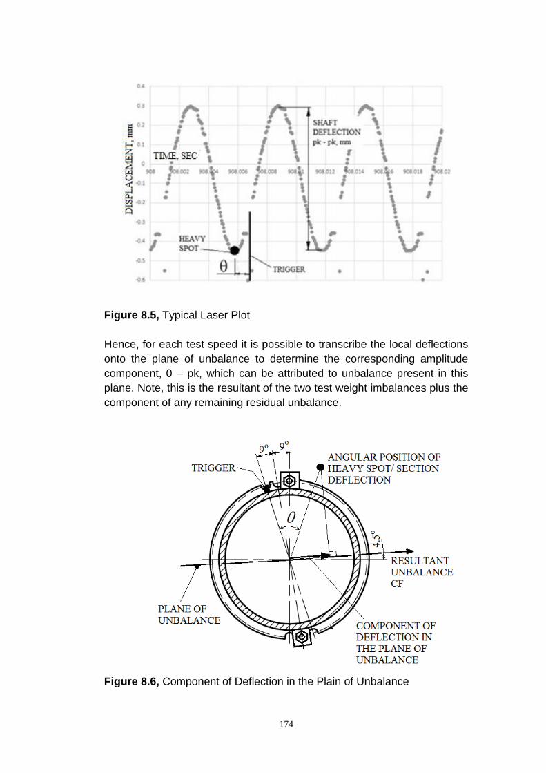
174
Figure 8.5, Typical Laser Plot
Hence, for each test speed it is possible to transcribe the local deflections
onto the plane of unbalance to determine the corresponding amplitude
component, 0 – pk, which can be attributed to unbalance present in this
plane. Note, this is the resultant of the two test weight imbalances plus the
component of any remaining residual unbalance.
Figure 8.6, Component of Deflection in the Plain of Unbalance
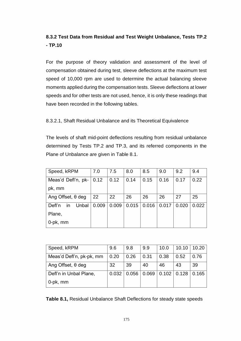
175
8.3.2 Test Data from Residual and Test Weight Unbalance, Tests TP.2
- TP.10
For the purpose of theory validation and assessment of the level of
compensation obtained during test, sleeve deflections at the maximum test
speed of 10,000 rpm are used to determine the actual balancing sleeve
moments applied during the compensation tests. Sleeve deflections at lower
speeds and for other tests are not used, hence, it is only these readings that
have been recorded in the following tables.
8.3.2.1, Shaft Residual Unbalance and its Theoretical Equivalence
The levels of shaft mid-point deflections resulting from residual unbalance
determined by Tests TP.2 and TP.3, and its referred components in the
Plane of Unbalance are given in Table 8.1.
Speed, kRPM 7.0 7.5 8.0 8.5 9.0 9.2 9.4
Meas’d Defl’n, pk-
pk, mm
0.12 0.12 0.14 0.15 0.16 0.17 0.22
Ang Offset, θ deg 22 22 26 26 26 27 25
Defl’n in Unbal
Plane,
0-pk, mm
0.009 0.009 0.015 0.016 0.017 0.020 0.022
Speed, kRPM 9.6 9.8 9.9 10.0 10.10 10.20
Meas’d Defl’n, pk-pk, mm 0.20 0.26 0.31 0.38 0.52 0.76
Ang Offset, θ deg 32 39 40 46 43 39
Defl’n in Unbal Plane,
0-pk, mm
0.032 0.056 0.069 0.102 0.128 0.165
Table 8.1, Residual Unbalance Shaft Deflections for steady state speeds
176
To determine a theoretical representation of the referred component of
residual unbalance, a Mathcad numerical program of a compensated shaft
with a single concentrated imbalance is compiled to calculate expected
balance characteristics from the analytical equations developed in Chapter
4 and using parameter values given in Table 8.2. These complied with the
mathematical model of the test shaft given in Chapter 6, but with the shaft
length increased to = 970 mm to give a critical speed of 10,750 rpm in
order to align it with the measured mean value of the two critical speeds
obtained from Test TP.11, (Forward and Backward Gyroscopic Critical
Speeds), as shown in Figure 8.12.
Through an iterative process, comparing theoretical and measured shaft
deflections in the plane of unbalance, a first order approximation of a
theoretical level of equivalent residual unbalance is assessed to be 50% of
the test weight unbalance, equal to 33.75 g.mm. Figure 8.7 shows this
provides a good relative comparison and is therefore subsequently added
to the test weight unbalance, thereby setting the theoretical level of
concentrated unbalance to 101.25 g.mm for the theory evaluation tests TP.4
to TP.10, and the results subsequently shown in Figures 8.9, 8.10 and 8.11.
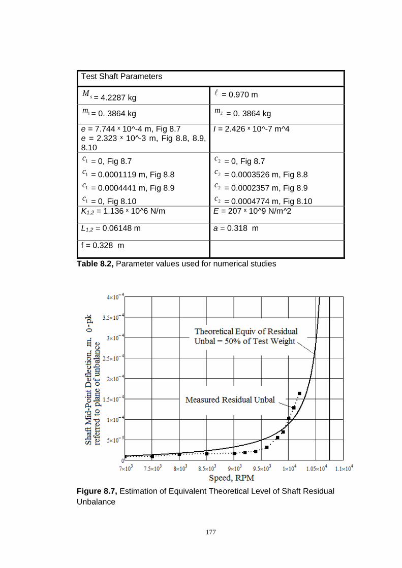
177
Table 8.2, Parameter values used for numerical studies
Figure 8.7, Estimation of Equivalent Theoretical Level of Shaft Residual
Unbalance
Test Shaft Parameters
sM= 4.2287 kg
= 0.970 m
1m = 0. 3864 kg 2m = 0. 3864 kg
e = 7.744 ˣ 10^-4 m, Fig 8.7 e = 2.323 ˣ 10^-3 m, Fig 8.8, 8.9, 8.10
I = 2.426 ˣ 10^-7 m^4
1c = 0, Fig 8.7
1c = 0.0001119 m, Fig 8.8
1c = 0.0004441 m, Fig 8.9
1c = 0, Fig 8.10
2c = 0, Fig 8.7
2c = 0.0003526 m, Fig 8.8
2c = 0.0002357 m, Fig 8.9
2c = 0.0004774 m, Fig 8.10
K1,2 = 1.136 ˣ 10^6 N/m E = 207 ˣ 10^9 N/m^2
L1,2 = 0.06148 m a = 0.318 m
f = 0.328 m
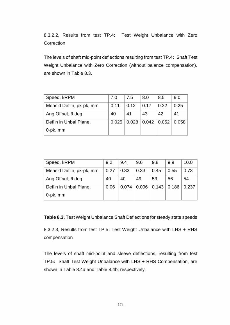
178
8.3.2.2, Results from test TP.4: Test Weight Unbalance with Zero
Correction
The levels of shaft mid-point deflections resulting from test TP.4: Shaft Test
Weight Unbalance with Zero Correction (without balance compensation),
are shown in Table 8.3.
Speed, kRPM 7.0 7.5 8.0 8.5 9.0
Meas’d Defl’n, pk-pk, mm 0.11 0.12 0.17 0.22 0.25
Ang Offset, θ deg 40 41 43 42 41
Defl’n in Unbal Plane,
0-pk, mm
0.025 0.028 0.042 0.052 0.058
Speed, kRPM 9.2 9.4 9.6 9.8 9.9 10.0
Meas’d Defl’n, pk-pk, mm 0.27 0.33 0.33 0.45 0.55 0.73
Ang Offset, θ deg 40 40 49 53 56 54
Defl’n in Unbal Plane,
0-pk, mm
0.06 0.074 0.096 0.143 0.186 0.237
Table 8.3, Test Weight Unbalance Shaft Deflections for steady state speeds
8.3.2.3, Results from test TP.5: Test Weight Unbalance with LHS + RHS
compensation
The levels of shaft mid-point and sleeve deflections, resulting from test
TP.5: Shaft Test Weight Unbalance with LHS + RHS Compensation, are
shown in Table 8.4a and Table 8.4b, respectively.
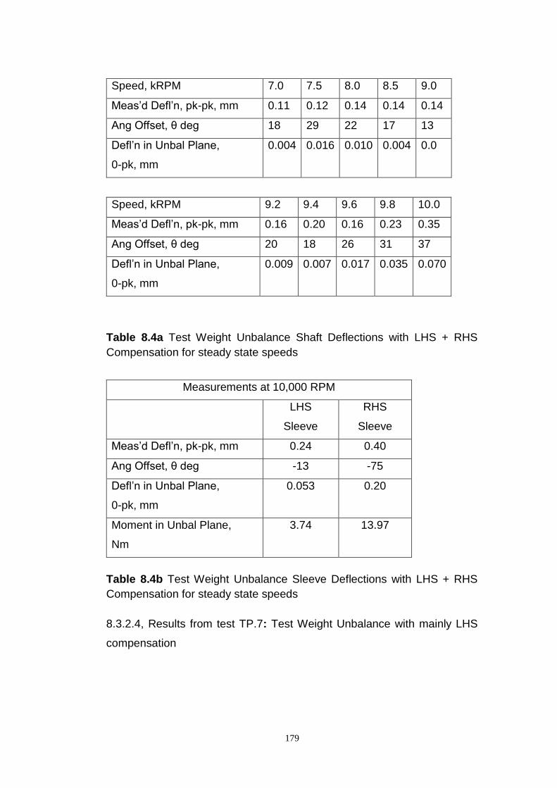
179
Speed, kRPM 7.0 7.5 8.0 8.5 9.0
Meas’d Defl’n, pk-pk, mm 0.11 0.12 0.14 0.14 0.14
Ang Offset, θ deg 18 29 22 17 13
Defl’n in Unbal Plane,
0-pk, mm
0.004 0.016 0.010 0.004 0.0
Speed, kRPM 9.2 9.4 9.6 9.8 10.0
Meas’d Defl’n, pk-pk, mm 0.16 0.20 0.16 0.23 0.35
Ang Offset, θ deg 20 18 26 31 37
Defl’n in Unbal Plane,
0-pk, mm
0.009 0.007 0.017 0.035 0.070
Table 8.4a Test Weight Unbalance Shaft Deflections with LHS + RHS
Compensation for steady state speeds
Measurements at 10,000 RPM
LHS
Sleeve
RHS
Sleeve
Meas’d Defl’n, pk-pk, mm 0.24 0.40
Ang Offset, θ deg -13 -75
Defl’n in Unbal Plane,
0-pk, mm
0.053 0.20
Moment in Unbal Plane,
Nm
3.74 13.97
Table 8.4b Test Weight Unbalance Sleeve Deflections with LHS + RHS
Compensation for steady state speeds
8.3.2.4, Results from test TP.7: Test Weight Unbalance with mainly LHS
compensation
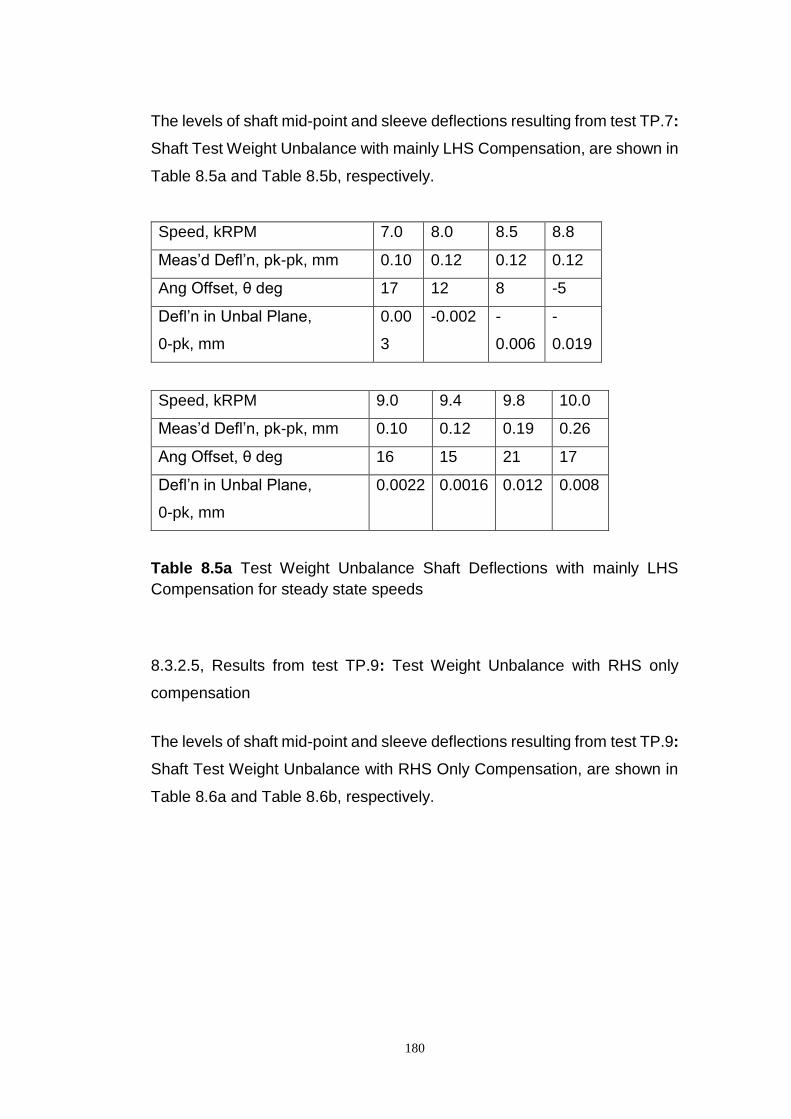
180
The levels of shaft mid-point and sleeve deflections resulting from test TP.7:
Shaft Test Weight Unbalance with mainly LHS Compensation, are shown in
Table 8.5a and Table 8.5b, respectively.
Speed, kRPM 7.0 8.0 8.5 8.8
Meas’d Defl’n, pk-pk, mm 0.10 0.12 0.12 0.12
Ang Offset, θ deg 17 12 8 -5
Defl’n in Unbal Plane,
0-pk, mm
0.00
3
-0.002 -
0.006
-
0.019
Speed, kRPM 9.0 9.4 9.8 10.0
Meas’d Defl’n, pk-pk, mm 0.10 0.12 0.19 0.26
Ang Offset, θ deg 16 15 21 17
Defl’n in Unbal Plane,
0-pk, mm
0.0022 0.0016 0.012 0.008
Table 8.5a Test Weight Unbalance Shaft Deflections with mainly LHS
Compensation for steady state speeds
8.3.2.5, Results from test TP.9: Test Weight Unbalance with RHS only
compensation
The levels of shaft mid-point and sleeve deflections resulting from test TP.9:
Shaft Test Weight Unbalance with RHS Only Compensation, are shown in
Table 8.6a and Table 8.6b, respectively.
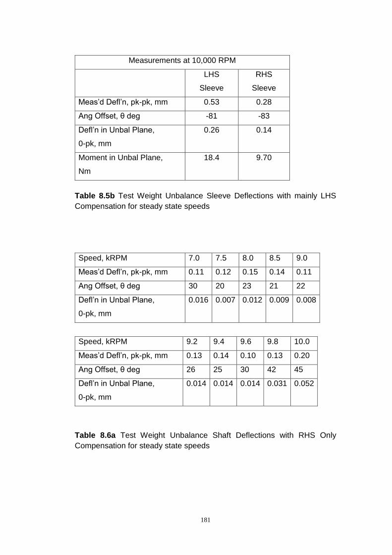
181
Measurements at 10,000 RPM
LHS
Sleeve
RHS
Sleeve
Meas’d Defl’n, pk-pk, mm 0.53 0.28
Ang Offset, θ deg -81 -83
Defl’n in Unbal Plane,
0-pk, mm
0.26 0.14
Moment in Unbal Plane,
Nm
18.4 9.70
Table 8.5b Test Weight Unbalance Sleeve Deflections with mainly LHS
Compensation for steady state speeds
Speed, kRPM 7.0 7.5 8.0 8.5 9.0
Meas’d Defl’n, pk-pk, mm 0.11 0.12 0.15 0.14 0.11
Ang Offset, θ deg 30 20 23 21 22
Defl’n in Unbal Plane,
0-pk, mm
0.016 0.007 0.012 0.009 0.008
Speed, kRPM 9.2 9.4 9.6 9.8 10.0
Meas’d Defl’n, pk-pk, mm 0.13 0.14 0.10 0.13 0.20
Ang Offset, θ deg 26 25 30 42 45
Defl’n in Unbal Plane,
0-pk, mm
0.014 0.014 0.014 0.031 0.052
Table 8.6a Test Weight Unbalance Shaft Deflections with RHS Only
Compensation for steady state speeds

182
Measurements at 10,000 RPM
LHS
Sleeve
RHS
Sleeve
Meas’d Defl’n, pk-pk, mm 0.031 0.60
Ang Offset, θ deg 4 -101
Defl’n in Unbal Plane,
0-pk, mm
0.0025 0.27
Moment in Unbal Plane,
Nm
0.18 19.07
Table 8.6b Test Weight Unbalance Sleeve Deflections with RHS Only
Compensation for steady state speeds
8.3.3 Bearing Reaction Loads
Although bearing reaction loads have not been directly measured during
these tests, assessments of their condition can be made from the results
given above. Figure 8.8 shows measurements of shaft mid-point
deflections, pk – pk mm, resulting from tests TP.4 to TP.10: (Test Weight
Unbalance, with and without balance compensation) in their plane of
measurement without any vector angle adjustment. Hence, disregarding the
external effect of the applied balancing sleeve CF on the reaction loads,
these provide a good approximation of the relative magnitudes of the
corresponding reaction loads that are seen by the shaft end bearings
resulting from the shaft’s bending/ internal shear forces.
It is also noted that these tests are conducted primarily to validate the
theoretical analysis of balancing sleeve compensation determined in earlier
chapters, and as a consequence the level of compensation has not been
optimised to minimise the reaction loads. Nevertheless, it is evident that
significant load reductions have occurred and that further reductions would
be possible by increased levels of compensation.

183
Figure 8.8, Comparison plots of Shaft Deflections, in their plane of
measurement, with and without Balance Compensation
8.3.4 Test and Theoretical Comparisons
To provide a valid comparison between theoretical shaft deflections and
their corresponding test results, the theoretical values of the LHS and RHS
compensating moments, Mo1 and Mo2, are matched to their respective test
quantities. The test moments are determined from the sleeve deflections, at
10,000 rpm, (adjudged to be sufficiently close to the critical speed for
comparison with the required moment for its elimination/ nullification),
multiplied by the sleeve stiffness and its length.
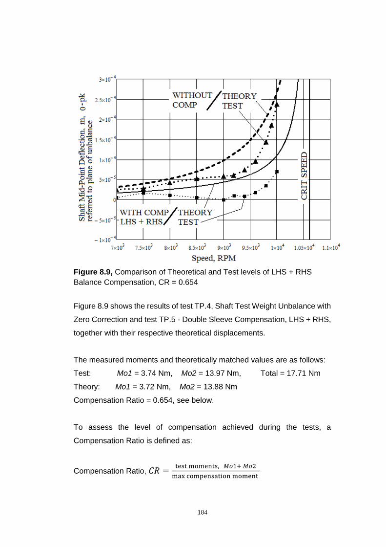
184
Figure 8.9, Comparison of Theoretical and Test levels of LHS + RHS
Balance Compensation, CR = 0.654
Figure 8.9 shows the results of test TP.4, Shaft Test Weight Unbalance with
Zero Correction and test TP.5 - Double Sleeve Compensation, LHS + RHS,
together with their respective theoretical displacements.
The measured moments and theoretically matched values are as follows:
Test: Mo1 = 3.74 Nm, Mo2 = 13.97 Nm, Total = 17.71 Nm
Theory: Mo1 = 3.72 Nm, Mo2 = 13.88 Nm
Compensation Ratio = 0.654, see below.
To assess the level of compensation achieved during the tests, a
Compensation Ratio is defined as:
Compensation Ratio, 𝐶𝑅 =test moments, 𝑀𝑜1+ 𝑀𝑜2
max compensation moment
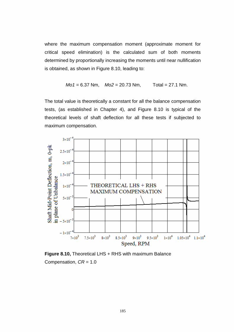
185
where the maximum compensation moment (approximate moment for
critical speed elimination) is the calculated sum of both moments
determined by proportionally increasing the moments until near nullification
is obtained, as shown in Figure 8.10, leading to:
Mo1 = 6.37 Nm, Mo2 = 20.73 Nm, Total = 27.1 Nm.
The total value is theoretically a constant for all the balance compensation
tests, (as established in Chapter 4), and Figure 8.10 is typical of the
theoretical levels of shaft deflection for all these tests if subjected to
maximum compensation.
Figure 8.10, Theoretical LHS + RHS with maximum Balance
Compensation, CR = 1.0

186
Figure 8.11, Comparison of Theoretical and Test levels of mainly LHS
Balance Compensation, CR = 1.037
Figure 8.11 shows results from test TP.4, Shaft Test Weight Unbalance with
Zero Correction and test TP.7 - Single Sleeve Compensation, mainly LHS,
(since some residual unbalance existed in the RHS) together with their
respective theoretical displacements.
The measured moments and theoretically matched values are as follows:
Test: Mo1 = 18.4 Nm, Mo2 = 9.7 Nm, Total = 28.1 Nm
Theory: Mo1 = 18.41 Nm, Mo2 = 9.74 Nm
Compensation Ratio = 1.037
Figure 8.12 compares the same test results of Figure 8.11 with their
theoretical equivalents without compensation, first with standard shaft
eccentricity, (concentrated unbalance = 101.25 g.mm, as per previous
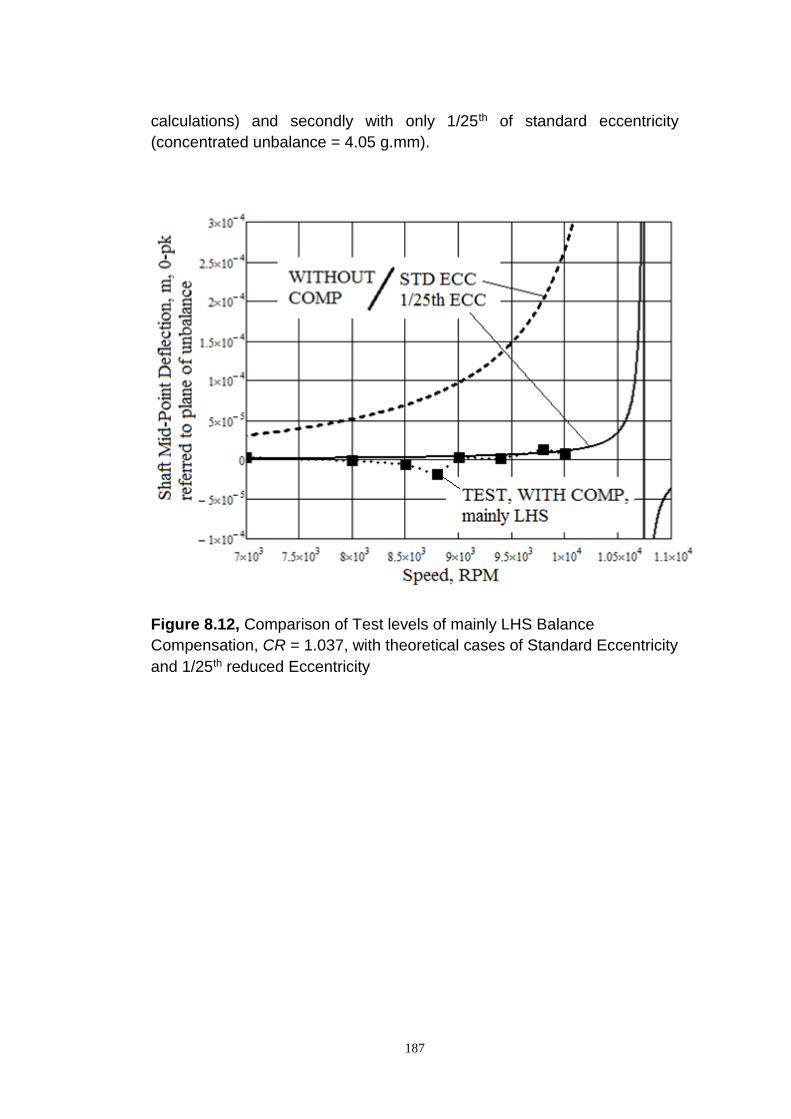
187
calculations) and secondly with only 1/25th of standard eccentricity
(concentrated unbalance = 4.05 g.mm).
Figure 8.12, Comparison of Test levels of mainly LHS Balance
Compensation, CR = 1.037, with theoretical cases of Standard Eccentricity
and 1/25th reduced Eccentricity
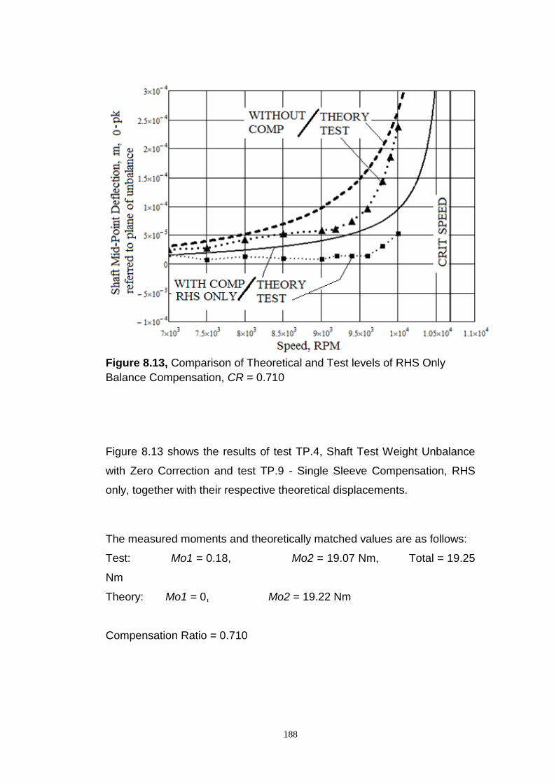
188
Figure 8.13, Comparison of Theoretical and Test levels of RHS Only
Balance Compensation, CR = 0.710
Figure 8.13 shows the results of test TP.4, Shaft Test Weight Unbalance
with Zero Correction and test TP.9 - Single Sleeve Compensation, RHS
only, together with their respective theoretical displacements.
The measured moments and theoretically matched values are as follows:
Test: Mo1 = 0.18, Mo2 = 19.07 Nm, Total = 19.25
Nm
Theory: Mo1 = 0, Mo2 = 19.22 Nm
Compensation Ratio = 0.710
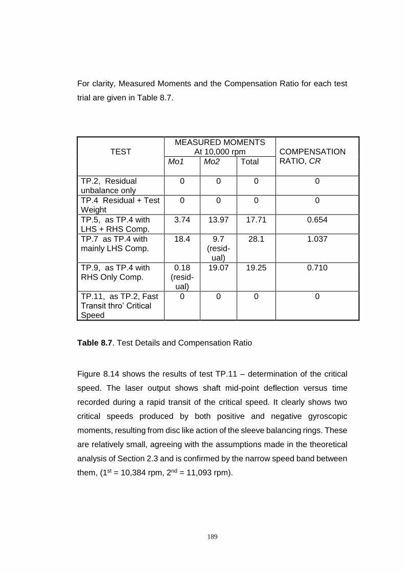
189
For clarity, Measured Moments and the Compensation Ratio for each test
trial are given in Table 8.7.
TEST
MEASURED MOMENTS At 10,000 rpm
COMPENSATION RATIO, CR Mo1 Mo2 Total
TP.2, Residual unbalance only
0 0 0 0
TP.4 Residual + Test Weight
0 0 0 0
TP.5, as TP.4 with LHS + RHS Comp.
3.74 13.97 17.71 0.654
TP.7 as TP.4 with mainly LHS Comp.
18.4 9.7 (resid-
ual)
28.1 1.037
TP.9, as TP.4 with RHS Only Comp.
0.18 (resid-
ual)
19.07 19.25 0.710
TP.11, as TP.2, Fast Transit thro’ Critical Speed
0 0 0 0
Table 8.7. Test Details and Compensation Ratio
Figure 8.14 shows the results of test TP.11 – determination of the critical
speed. The laser output shows shaft mid-point deflection versus time
recorded during a rapid transit of the critical speed. It clearly shows two
critical speeds produced by both positive and negative gyroscopic
moments, resulting from disc like action of the sleeve balancing rings. These
are relatively small, agreeing with the assumptions made in the theoretical
analysis of Section 2.3 and is confirmed by the narrow speed band between
them, (1st = 10,384 rpm, 2nd = 11,093 rpm).
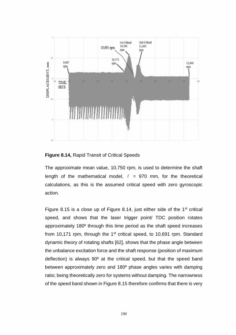
190
Figure 8.14, Rapid Transit of Critical Speeds
The approximate mean value, 10,750 rpm, is used to determine the shaft
length of the mathematical model, = 970 mm, for the theoretical
calculations, as this is the assumed critical speed with zero gyroscopic
action.
Figure 8.15 is a close up of Figure 8.14, just either side of the 1st critical
speed, and shows that the laser trigger point/ TDC position rotates
approximately 180º through this time period as the shaft speed increases
from 10,171 rpm, through the 1st critical speed, to 10,691 rpm. Standard
dynamic theory of rotating shafts [62], shows that the phase angle between
the unbalance excitation force and the shaft response (position of maximum
deflection) is always 90º at the critical speed, but that the speed band
between approximately zero and 180º phase angles varies with damping
ratio; being theoretically zero for systems without damping. The narrowness
of the speed band shown in Figure 8.15 therefore confirms that there is very

191
little damping in the test set-up, and consequently the measurement
orientation shown in Figure 8.4 is fit for purpose.
Figure 8.15, Trigger Rotation through the 1st Critical Speed
8.4 Preliminary Conclusions
Tests are conducted with the primary aim of checking the practical validity
of the theory/conclusions resulting from the preceding chapters and are
therefore not optimised for maximum possible balance compensation in this
192
instance. However, it is possible to draw very strong conclusions from the
results, namely:
1. Tests including balance sleeve compensation, Figure 8.9, Figure
8.11 and Figure 8.12, show that the shaft mid-point deflections have
been reduced from their zero balance condition without
compensation as speed increases up to the maximum test speed of
10,000 rpm, (93% of the mean critical, 96% of the 1st forward mode).
Consequently, it has been demonstrated that balance sleeve
compensation definitely performs as expected and the condition of
shaft balance is improved.
2. The preceding tests show a good correlation between reductions in
shaft deflection and their corresponding Compensation Ratio, CR,
such that the closer CR is to 1.0, the less bending of the shaft occurs
and the better the condition of shaft balance. Figure 8.11 with CR =
1.037 is particularly significant, having near maximum compensation
and a very close alignment with predicted theory. Hence, the tests
strongly support the principle of the new balancing methodology of
aligning the sum of the sleeve balancing moments to the sum of the
equivalent encastre fixing moments.
3. Figure 8.13, with RHS (only) balance compensation (the small LHS
compensating moment, due of residual imbalance within the
balancing ring is of negligible proportions) confirms the conclusions
of Chapter 4 that compensation/ balance adjustment need only be
applied at one end of a shaft.
4. Figure 8.12, shows that when compensation is close to maximum,
CR = 1.037, the balance condition is equivalent to reducing the
amount of residual unbalance by 1/25th of its original value. This test
confirms the theoretical analysis given in Chapter 5, reference: Shear

193
Force Reaction Ratio, RR, Figure 5.2 and the equivalent reduction in
standard eccentricity, shown in Figure 5.16. Chapter 5 also shows
that the Reaction Ratio, RR, is independent of shaft eccentricity such
that the benefits of encastre simulation apply to any pre-determined
level of residual eccentricity. It is therefore concluded that these
balancing gains should be possible even on previously balanced
shafts. Therefore, the potential exists to vastly reduce shaft
imbalance and hence to safely operate high-speed machinery much
closer to its lateral critical speed than is currently allowed.
194
Chapter 9
9.1 Conclusions
This research resulted from industrial balancing problems encountered by
certain turbine/ compressor packages, employing flexible, high-speed
coupling shafts; which determined the need for an examination into currently
available balancing techniques, coupled with an investigation into possible
ways of reducing the consequentially high level of reaction loads imposed
on shaft bearings.
The work successfully formulated the requirements of a new balancing
technique with the potential to vastly reduce the reaction loads imparted on
shaft end bearings, and it has also uncovered several beneficial insights
into the controlling mechanism of the methodology.
Chapter 2 showed that by applying trim balance correction directly onto
rotating shafts, as per existing balancing methodologies, that their
effectiveness reduces with increased shaft speed/ bending deflection. This
is because the rotational radius of their mass centroid, remains either
constant, or possibly reduces, depending on its lengthwise position along
the shaft, whereas the equivalent radius of shaft imbalance increases.
Hence, a balancing error is created, as a result of the rigidity of the trim
balance mass.
To counter this problem, chapter 2 further describes a new concept of
adding compliance to a trim balancing mechanism such that amplification of
the correcting forces occurs by the use of a pair of compensating balancing
sleeves. This also has the added benefit of imparting balancing moments
onto the shaft, acting to reduce its deflection. This effect is investigated by
dynamic analysis of a simply supported, high-speed, plain, flexible shaft,
195
with uniform eccentricity, which concluded that considerable reductions in
both reaction loads and shaft deflection are possible.
It is also shown that the balancing moments enable the theoretical
elimination of the 1st classical, critical speed and chapter 3 shows that
nullification of a neighbouring compensating critical speed is also possible
by closely matching the balancing moments to the fixing moments of an
equivalent encastre mounted shaft. This requirement then forms the
essence of a new balancing methodology whereby reaction loads and shaft
deflections are reduced by the process of encastre simulation.
Further insights are revealed by the analysis given in Chapters 4, which
shows that it is the sum of the balancing moments that produce nullification
and this can be achieved by the use of a single compensating balance
sleeve fitted at either end of the shaft, thereby replicating a single encastre
shaft.
The applicability of the new methodology to the majority of practical shafts,
with any distribution of concentrated imbalances and/ or multiple discs,
provided they are mounted within the central 80% of the shaft length, is
demonstrated in chapter 5.
Further, analysis of the shear force reaction ratio, RR, showed it to be
independent of the shaft eccentricity, hence the reduction in the equivalent
shaft eccentricity, made possible by this methodology, is in addition to any
balance reductions that may have been made prior to encastre simulation;
for example by, component and/ or assembly balancing procedures. It is
shown that these reductions are as high as 25x at operations close to the
1st critical speed, hence, extremely low levels of equivalent eccentricity are
possible.

196
Chapter 5, also shows that the magnitude of a Simulation Ratio, SR,
provides a good indication of shaft stiffening effects produced by balance
sleeve compensation and hence, that double encastre simulation, could be
beneficially applied to shafts operating at higher critical speeds.
The potential balancing improvements and practical insights revealed in
these chapters are strongly supported by the validating test results reported
in chapter 8. These confirm that:
1. shaft mid-point deflections and by association, shaft end reaction
loads can be considerably reduced by applying balancing sleeve
compensation,
2. the Compensation Ratio, CR is a good indicator of shaft balance,
such that the closer CR is to 1.0, the less bending of the shaft occurs,
confirming the requirement to closely align the sum of the sleeve
balancing moments to the sum of the equivalent encastre fixing
moments,
3. balance compensation/ adjustment can be successfully performed at
a single shaft end,
4. with compensation close to its maximum (test value CR = 1.037) the
balance condition is equivalent to reducing the amount of residual
unbalance by 1/25th of its original value.
It is therefore concluded that balancing sleeve compensation has been
proven to work satisfactorily under laboratory conditions, but further work
would be required if commercial acceptance is to be obtained, requiring site
testing of a full sized prototype.
197
It is realised that encastre simulation, by application of balancing sleeve
moments, could be achieved by a large variety of designs and bending
mechanisms. Hence, it is possible that different drive train arrangements
would be better served by a particular balancing sleeve design, some
examples of which are discussed below.
For external application, high bending stiffness of a large, tubular sleeve
can be problematic and its reduction by machining of axial slots, to produce
a number of spars, as per the test shaft, may not be the best method. As an
alternative, many composite designs are possible, including materials with
a lower Young’s Modulus, such as plastic, titanium, aluminium etc.,
combined with an inbuilt, heavier material, balancing ring.
A further patented alternative [120] shown in Figure 9.1, makes use of
laminated, flexible, disc elements, item (95), as commonly used in high
speed drive coupling applications, (as per the test shaft). These are
therefore of proven design and are commercially available in several pack
sizes so that the bending stiffness could be set accordingly by varying the
number of laminations. The method of element fastening is a standard
feature of these types of flexible couplings to allow for angular misalignment
and is therefore an ideal, low cost method of adding an angular stiffness
component to the balancing sleeve (97). Hence, it is not necessary to
reduce the bending stiffness of the sleeve as in previous designs for
external applications.

198
Figure 9.1, Alternative Balancing Sleeve Design for external application
Where space is available, designs for internal applications, preferably with
external adjustment, would appear to be advantageous, offering zero
additional windage (drag caused by shaft rotation) and because of the
reduction in sleeve diameter, lower bending stiffness. One such patent
pending design [124] is shown in Figure 9.2.
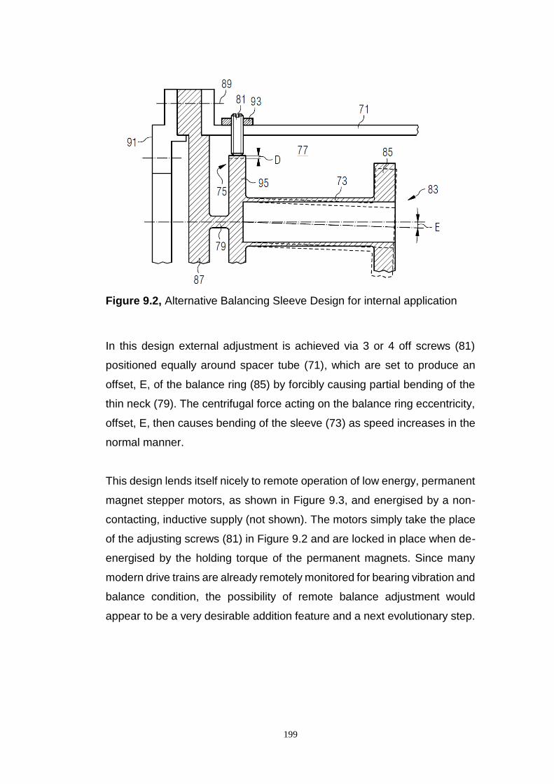
199
Figure 9.2, Alternative Balancing Sleeve Design for internal application
In this design external adjustment is achieved via 3 or 4 off screws (81)
positioned equally around spacer tube (71), which are set to produce an
offset, E, of the balance ring (85) by forcibly causing partial bending of the
thin neck (79). The centrifugal force acting on the balance ring eccentricity,
offset, E, then causes bending of the sleeve (73) as speed increases in the
normal manner.
This design lends itself nicely to remote operation of low energy, permanent
magnet stepper motors, as shown in Figure 9.3, and energised by a non-
contacting, inductive supply (not shown). The motors simply take the place
of the adjusting screws (81) in Figure 9.2 and are locked in place when de-
energised by the holding torque of the permanent magnets. Since many
modern drive trains are already remotely monitored for bearing vibration and
balance condition, the possibility of remote balance adjustment would
appear to be a very desirable addition feature and a next evolutionary step.
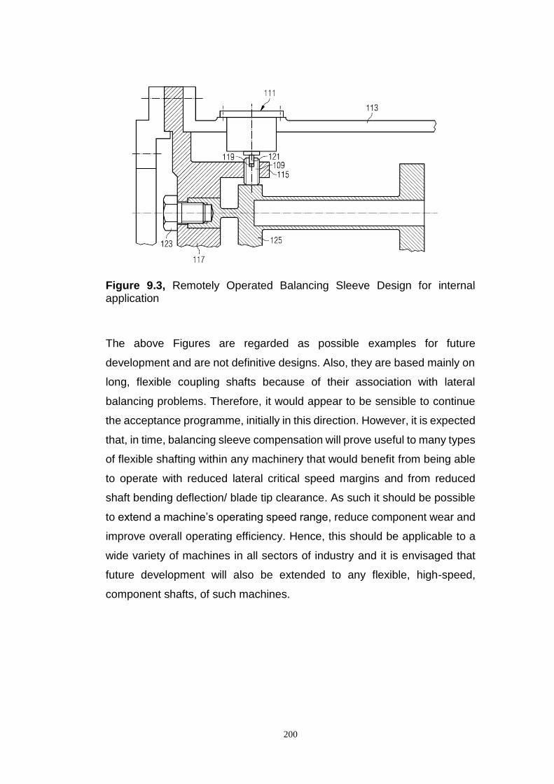
200
Figure 9.3, Remotely Operated Balancing Sleeve Design for internal application
The above Figures are regarded as possible examples for future
development and are not definitive designs. Also, they are based mainly on
long, flexible coupling shafts because of their association with lateral
balancing problems. Therefore, it would appear to be sensible to continue
the acceptance programme, initially in this direction. However, it is expected
that, in time, balancing sleeve compensation will prove useful to many types
of flexible shafting within any machinery that would benefit from being able
to operate with reduced lateral critical speed margins and from reduced
shaft bending deflection/ blade tip clearance. As such it should be possible
to extend a machine’s operating speed range, reduce component wear and
improve overall operating efficiency. Hence, this should be applicable to a
wide variety of machines in all sectors of industry and it is envisaged that
future development will also be extended to any flexible, high-speed,
component shafts, of such machines.

201
References
[1] Dunkerley S. On the Whirling and Vibration of Shafts. Phil Trans
Roy Soc , London, Series A 1894;185.
[2] Jeffcott HH. The lateral vibration of loaded shafts in the
neighbourhood of a whirling speed. - The effect of want of balance.
Philosophical Magazine 1919;6:37:304-314.
[2a]
[3]
Cerminaro A.M. Simulation of Internal Damping in a Rotating
System supported by Magnetic Bearings. MSc Thesis, Tuffs
University, 1999.
Rankine W. On the Centrifugal Force of Rotating Shafts. Engineer,
London 1869;247:249.
[4] Prabhakar S, Sekhar A.S, Mohanty A.R. Vibration analysis of a
misaligned rotor-coupling-bearing system passing through the
critical speed. Proc Instn Mech Engrs Vol 215, 2001.
[5] Stodola A. Steam and gas turbines. McGraw-Hill, New York. English
translation, 1927.
[6] Campbell W. The protection of steam-turbine disk wheels from axial
vibration. Trans. ASME, 1924.
[7] Kimball, A. L. Vibration preventionin engineering. J. Wiley & Sons.
London 1932
[8] Newkirk B.L. Shaft whipping/ rubbing/ whirling. General Electric
Rev. 27,28. 1924-1926.
[9] Nelson F. Damping in structural analysis and design, impact and
friction solids, structures and machines. Birkhauser In Press, 1999.
[10] Kramer E. Dynamics of rotors and foundations. Springer-Verlag
Berlin Heidelberg. 1993.
[11] Dimarogonis A. D. Analytical methods in rotor dynamics. Applied
science publishers, London, 1983.
[12] Ehrich F.F. Shaft whirling induced by rotor internal damping. Journal
of applied mechanics. 1964.
[13] Robertson D. Hysteretic influences on whirling of rotors. Proc. Of
the Inst. Of Mech. Eng. 1935.
202
[14] Smith D.M. The motion of a rotor carried by a flexible shaft in flexible
bearings. Proc. Royal Society, London. 1933.
[15] Special Purpose Couplings for Petroleum, Chemical and Gas
Industry Services. API Standard 671. 4th ed. 2007
[16] Mancuso J.R. The manufacturer's world of coupling potential
unbalance. Kop-Flex Emerson Power Transmission Corp, JRM
10.PDF. 1985 circa.
[17] ISO 1940-1:2003. Balance quality requirements for rotors of
constant (rigid) state.
[18] ISO 1940-2:1997. Mechanical vibration. Balance quality
requirements for rigid rotors. Balance errors.
[19] Gas turbines for the petroleum, chemical and gas industry services.
API 616. 4th ed. 1998.
[20] Recommended practice for packaged combustion gas turbines. API
RP 11PGT:1992
[21] 100 years of balancing technology, Schenck USA, www.schenck-
usa/company/information/history.php
[22] ISO 5406-1980. The mechanical balancing of flexible rotors.
[23] ISO 7919-4 2nd Edition 2009-10-01 Mechanical Vibration –
Evaluation of machine vibration by measurements on rotating shafts
: Part 4 Gas turbines sets with fluid-film bearings.
[24] ISO 10816-4 2nd Edition 2009-10-01 Mechanical Vibration –
Evaluation of machine vibration by measurements on non-rotating
shafts : Part 4 Gas turbines sets with fluid-film bearings.
[25] Bishop R. Gladwell G. The vibration and balancing of an unbalanced
flexible rotor. IMechE Part C: J Mechanical Engineering Science
1959; 1: 66-77
[26] Bishop R. The Vibration of Rotating Shafts. IMechE Part C: J.
Mechanical Engineering Science 1959; 1: 50-65
[27] Corcoran JP. What is Acceptable Coupling Lateral Critical Speed?
Turbomachinery International 2003; May/ June: 18-21.
203
[28] Garvey SD, Friswell MI, Williams EJ, Care ID. Robust balancing for
rotating machines. IMechE Part C: J Mechanical Engineering
Science 2002; 216: 1117-1130.
[29] Gladwell G, Bishop R. The vibration of rotating shafts in flexible
bearings. IMechE Part C: J Mechanical Engineering Science
1959;1:195-206.
[30] Hylton PD. Low Speed Balance for Supercritical Shafting in Gas
Turbines. Proceedings of ASME Turbo Expo 2008: Power for Land,
Sea and Air, Berlin, Germany, 9-13 June 2008; Paper Number
GT2008-50077. New York: ASME.
[31] Morton PG. Modal balancing of flexible shafts without trial weights
IMechE Part C:J Mechanical Engineering Science 1985;199:71-78.
[32] Parkinson AG. Balancing of rotating machinery. IMechE Part C: J
Mechanical Engineering Science 1991; 205: 53-66.
[33] Parkinson A.G, Bishop R.E.D. Residual vibration in modal
balancing. Journal Mechnical Science. 1965
[34] Yu JJ. On two plane balancing of symmetric rotors. Proceedings of
ASME Turbo Expo 2012 2012
[35] Genta G. Dynamics of Rotating Systems, Springer, Mechanicak
Engineering Series, 2005
[36] Sergio G. Torres Cedillo. Unbalanced identification and balancing
of nonlinear rotordynamic systems. Proc of ASME Turbo Expo,
GT2014-25290
[37] Genta G, Silvagni M. On centrifugal softening in finite element
method rotordynamics, Journal of applied mechanics. ASME Jan
2004 Vol 81/ 011001-1
[38] Nelson F. Rotor dynamics without equations. Int journal of
COMADEM, 10(3) july 2007,PP.2-10
[39] Nandi A, Neorgy S. Modelling of rotors with three-dimensional solid
finite elements. Journal of strain analysis. Vol 36. No4. 2001.
204
[40] Black H.G. Lateral vibration of shafts having radial symmetry and
appreciable gyro action. Journal of mechanical engineering science.
Vol 6, 1964.
[41] Saldarriaga M. V, Steffren V, Hagopian J, mahfoud J. On the
balancing of flexible rotating machines by using an inverse problem
approach. Journal of vibration and control. 2010
[42] Lees A.W, Friswell M.I. The evaluation of rotor imbalance in flexibly
mounted machines. Journal of sound and vibration. 1997.
[43] Xiaofeng L, Longxi Z, Zhenxia L. Balancing of rotors without trial
weights based on finite element modal analysis. Journal of sound
and vibration. 2012.
[44] El-Shafei A,El-Kabbany A.S, Younan A.A. Rotor balancing without
trial weights. Trans ASME, July 2004.
[45] Racic Z, Hidalgo J. Practical balancing of flexible rotors for power
generation. Proc ASME 2007 Int Des Eng Tech Conf. DETC2007-
34333.
[46] Nicholas J.C, Gunter E.J, Allaire P.E. Effect of residual shaft bow
on unbalance response and balancing of a single mass flexible
rotor. Journal of engineering gas turbines power. 1976.
[47] Edwards S, Lees A.W, Friswell M.I. Fault diagnosis of rotating
machinery. Shock and vibration digest. 1998.
[48] Gunter E.J, Barrett L.E, Allaire P.E. Balancing of multimass flexible
rotors. Proc. 5th Turbomachinery Symposium. 1976.
[49] Sinha J.K, Friswell M.I, Lees A.W, Sinha R.K. Robust method for
the rotor unbalance estimation. Proc. VECTOMAC-2, 2002.
[50] Thearle E.L. Dynamic balancing of rotating machinery in the field.
Proc. ASME 1934.
[51] Zhao Q.L, Wang H.Q, Yao J.F. A novel method of dynamic balance
weighting for single-disc rotor system. WSEAS trans. On systems.
2012.
[52] Kellenberger W. Should a flexible rotor be balanced in N or (N+2)
planes. Journal Manuf. Sci. Eng. 1972.

205
[53] Hundal M.S, Harker R.J. Balancing of flexible rotors having arbitrary
mass and stiffness distribution. Journal of Engineering for Industry.
1966.
[54] Zang C, Lees A.W, Friswell M.I. Multi plane balancing of a rotating
shaft using a single transducer. IFToMM 6th Conference on Rotor
Dynamics. 2002
[55] Goodman T.P. A least squares method for computing balance
corrections. ASME Journal of Engineering for Industry. 1964
[56] Green R.B. Gyroscopic effects on the critical speeds of flexible
rotors. Journal Applied Mechanics, trans. Amer. Soc. Mech. Engrs.
1948
[57] Saravanamuttoo HIH. Rogers GFC. Cohen H. Straznicky PV. Gas
Turbine Theory. 6th ed. Harlow: Pearson Education Limited 2009
[58] Thomson WT. Mechanical Vibrations. 4th ed. London: Chapman &
Hall 1996
[59] Friswell M, Penney J, Garvey S, Lees A. Dynamics of rotating
machines. New York: Cambridge University Press, 2010.
[60] Rhyder GH. Strength of Materials. 3rd ed. Basingstoke: Macmillan
Press. 1992.
[61] Timoshenko S, Young DH, Weaver Jr W. Vibration problems in
engineering. : John Wiley and Sons, 1974
[62] Wilcox JB. Dynamic Balancing of Rotating Machinery. London:
Pitman. 1967.
[63] De Jong F.M.Application of a heat barrier sleeve to prevent
synchronous rotor instability, Proc Turbomachinery Symposium,
1998
[64] Sloetjes P.J. Vibration reduction and power generation with
piezoceramic sheets mounted to a flexible shaft. Journal of
Intelligent Material Systems and Structures, Vol. 19, Jan 2008
[65] Marin M.A. Rotor dynamics of overhung rotors: hysteretic dynamic
behavior. Proc of ASME Turbo Expo, GT2012-68285
206
[66] Al-Khazali H.A, Askari M. Modal analysis design to exposure
gyroscopic effect in rotating machinery using experimental and
analytical/ computational techniques. Int journal Eng Science &
tech, (IJEST), Vol 3, Sept 2011.
[67] Feese T.D, Grazier P.E. Balance this! Case histories from difficult
to balance jobs. Proc Turbomachinery Symposium, Sept 2004.
[68] Childs D.W, Vance J.M. Annular gas seals and rotordynamics of
compressors and turbines. Proc Turbomachinery Symposium,
1997.
[69] Zhang Q. Study of the stiffness loss and its affecting factors of the
spline joint used in rotor systems. Proc of ASME Turbo Expo,
GT2014-26876
[70] Weimeng MA. Dynamic analysis of asymmetric rotor bearing
system based on three dimensional finite element method. Proc of
ASME Turbo Expo, GT2014-25304
[71] Dutt J.K, Nakra B.C. Dynamics of rotor shaft system on flexible
supports with gyroscopic effects. Mech Research Communications,
Vol 22, 1995. Pergamon.
[72] Sinou J.J, Villa C, Thouverez F. Experimental and numerical
investigations of a flexible rotor bearing supports. Int journal of
rotating machines. 2005:3
[73] Werner U. Mathematical rotordynamic model regarding excitation
due to elliptical shaft journals in electrical motors considering the
gyroscopic effect. Applied Mathematics, 2013, 4, 57-74. Scientific
Research.
[74] Greenhill L.M. Lease V.J. Additional investigations into natural
frequencies and critical speeds of a rotating, flexible shaft-disk
system. Proc of ASME Turbo Expo, GT2007-28065
[75] Edwards S, Lees A.W, Friswell M.I. The influence of torsion on rotor/
stator contact in rotating machinery. Journal of sound and vision.
1999

207
[76] Madden R.J, Sawicki J.T, Pesch A.H. Model validation for
identification of damage dynamics. Proc of ASME Turbo Expo 2014,
GT2014-27341
[77] Wu X, Meagher J. A two-disc extended Jeffcott rotor model
distinguishing a shaft crack from other rotating asymmetries. Int
journal of rotating machinery. 2008.
[78] Chattoraj C. Whirling of a rotor on isotropic shaft considering
gyroscopic effects and asymmetric bearing stiffness. NaCoMM-
09Paper ID: DVAMCC1.
[79] Shiau T.N. Nonlinear dynamic study on effects of rub-impact caused
by oil rupture in a multi-shaft turbine with a squeeze damper. Proc
of ASME Turbo Expo, GT2014-27221
[80] Zilli A. Non-linear dynamics of a simplified model of an overhung
rotor subjected to intermittent annular rubs. Proc of ASME Turbo
Expo, GT2014-26826.
[81] Wang C. Study of stiffness loss and the dynamic influence on rotor
system of the bolted flange joint. Proc of ASME Turbo Expo,
GT2014-26191
[82] Aleyaasin M, Ebrahimi M, Whalley R. Multi-mass rotating shaft
analysis and identification. IMechE Part K: Proc Instn Mech Engrs
Vol 213, 1999
[83] De Jong F.M, Morton P.G. The synchronous instability of a
compressor rotot due to bearing journal differential heating. Trans
ASME Vol 118, Oct 1996
[84] Whalley R, Ebrahimi M, Abdul-Ameer A. High-speed rotor-shaft
systems and whirling identification. IMechE Part C: J. Mechanical
Engineering Science 2007, Vol 221
[85] Swanson E, powell C.D, Weissman S. A practical review of rotating
machinery critical speeds and modes. Sound and Vibration, May
2005.
208
[86] Tadeo A.T, Cavalca K.L, Brennan M.J. Dynamic characterization of
a mechanical coupling for a rotating shaft. IMechE Part C: J.
Mechanical Engineering Science 2010, Vol 225
[87] Varun Kumar M, Ashiwini kumar B. Model analysis of axially
symmetric linear rotating structures. Int Journal of Eng & Advanced
Technology, (IJEAT). Vol-2, Iss-4 April 2013.
[88] Mushi S.E, Lin Z, Allaire P.E, Evans S. Aerodynamic cross-coupling
in a flexible rotor: control design and implementation. 11th Int
Symposium on magnetic bearings. Aug 26-29, Nara, Japan.
[89] Adams M.L. Rotating machinery vibration from analysis to
troubleshooting. New York. Marcel Dekker Inc. 2001.
[90] Rao J.S. A note on Jeffcott warped rotor. Mechanism and machine
theory. Pergamon. Jan 2001.
[91] Mushi S.E, Lin Z, Allaire P.E. Design, construction and modeling of
a flexible rotor active magnetic bearing test rig. Proc of ASME Turbo
Expo, GT2010-23619.
[92] Samantaray A.K. Steady-state dynamics of a non-ideal rotor with
internal damping and gyroscopic effects. Nonlinear Dyn (2009)
56:443-451, DOI 10.1007/s11071-008-9413-8, Sprnger.
[93] Rodrigues DJ. Champneys AR, Friswell MI, Wilson RE. Automatic
balancing of a rigid rotor with misaligned shaft. Applied Mechanics
and Materials 2006; 5-6: 231-236
[94] Jerzy T. Sawicki. Stability of cracked rotor subjected to parametric
excitation. Proc of ASME Turbo Expo, GT2014-26741
[95] Horst H.G., Wolfel H.P. Active vibration control of a high speed rotor
using PZT patches on the shaft surface. Journal of Intelligent
Material Systems and Structures, Vol. 15, Sept 2004.
[96] Greenhill L.M, Cornejo G.A.Critical speeds resulting from unbalance
excitation of backward whirl modes. Design Eng Tech Conf. Vol 3-
Part B, ASME 1995.
[97] Gosiewski Z. Analysis of coupling mechanism in lateral/ torional
rotor vibrations. Journal of theoretical and applied mechanics. 2008
209
[98] Zhou S, Shi J. Active balancing and vibration control of rotating
machinery: A survey. The shock and vibration digest. Vol 33. No 4.
2001.
[99] Saldarriaga M. V, Steffren V. Balancing of flexible rotors without trial
weights by using optimisation techniques. Proc of COBEM 2003
[100]
Alauze C, Der Hagopian J, Gaudiller L. Active balancing of
turbomachinery: application to large shaft lines. Journal of vibration
and control. 2001.
[101] Ehyaei J, Moghaddam M.M. Dynamic response and stability
analysis of an unbalanced flexible rotating shaft equipped with n
automatic ball-balancers. Journal of sound and vibration. 2008.
[102] Rodrigues D, Champneys A, Friswell M, Wilson E. A consideration
of support asymmetry in an automatic ball balancing system. ENOC
2008.
[103] Foppl. A, Das problem der Laval'schen turbinenwelle. Civil
Ingenieur, 1895.
[104] Levine W. S. Control Systems fundamentals. CRC Press. 1999
[105] Nataraj C. vibration of mechanical systems. Cengage Learning.
2012.
[106] Green W.G. Theory of machines. Blackie & sons. London/ Glasgow.
1964.
[107] Muszynska A. Lateral-torsional vibrations of a rotor. BRDRC Report
No. 2, 1984.
[108] Vance J. M. Rotodynamics of turbomachinery. John Wiley &
Sons.1988
[109] Balachandran B, Magrab E.B. Vibrations. Cengage Learning. 2009.
[110] Broch J.T. Mechanical vibration and shock measurements. Bruel &
Kjaer. 1980.
[111] McConnell K.G. Vibration testing, theory and practice. John Wiley &
Sons. 1995.
210
[112] Langthjem M.A, Nakamura T. Dynamics of the fluid balancer:
Perturbation solution of a forced Korteweg-de vries-burgers
equation.
[113] Lees A.W, Sinha J.K, Friswell M.I. The identification of the
unbalance of a flexible rotating machine from a single run-down.
Proc of Turbo Expo, 2002, GT-2002-30420.
[114] Burrows CR. Keogh PS. Sahinkaya MN. Progress towards smart
rotating machinery through the use of active bearings. IMechE Part
C: J Mechanical Engineering Science 2009; 223: 2849-2859
[115] Yoon S.Y. Control of surge in centrifugal compressors by active
magnetic bearings. Advances in industrial control, DOI
10.1007/978-1-4471-4240-9_2, Springer-Verlag London 2013
[116] Bonello P. Adaptive tuned vibration absorbers: design principles,
cocepts and physical implementation. Vibration analysis and control
- new trends and developments. Intech, 2011.
[117] Kirk A, Knowles G, Stewart J Bingham C. Mathematical
development and modelling of a counter balance compensating
sleeve for the suppression of lateral vibrations in high speed flexible
couplings” ASME Turbo Expo San Antonio, TX, 3-7 June 2013;
Paper number GT2013-95634. New York: ASME.
[118] Knowles G, Kirk A. Theoretical investigation into balancing high-
speed flexible-shafts, by the use of a novel compensating balancing
sleeve. IMechE Part C: J Mechanical Engineering Science 2013;
Article No. 517376.
[119] Knowles G, Kirk A, Bingham C. Bickerton R. Generalised analysis
of compensating balancing sleeves with experimental results from
a scaled industrial turbine coupling shaft. IMechE Part C: Journal
of Mechanical Engineering Science - submitted 2016; Knowles G,
Kirk A, Bingham C, Bickerton R, - PENDING
[120] Knowles G. An apparatus comprising a shaft and a balancing
sleeve. European Patent EP2226529B1. 2012.

211
[121] Knowles G. An apparatus comprising a shaft and a balancing
sleeve. United States Patent US8556738B2. 2012.
[122] Knowles G. An apparatus comprising a shaft and balancing
device. European Patent EP2568194A1. 2013.
[123] Knowles G. An apparatus comprising a shaft and a balancing
device for balancing the shaft. European Patent EP2703689A1.
2014.
[124] Knowles G. An apparatus comprising a shaft and a compensator
balancing sleeve for balancing the shaft. European Patent
EP2806186A1. 2014.

212
Appendix A
Partial Fractions: Ref. Chapter 2, Section 2.3
44
2
44
2
1
44
1
44
4
)( bs
A
bs
sr
bs
sA
bss
ebr
(2.21a)
The Laplace equation for the combined assembly, (2.21a), can be
expanded, by the use of Partial Fractions, so as to express each term into
a standard Laplace form as follows:
For the 1st term, let:
bs
E
bs
D
bs
CBs
s
A
bsbsbss
eb
bss
eb
2222
4
44
4
))()(()(
Then, equating numerators gives:
))(()())()(( 224 bsbssCBsbsbsbsAeb
))(())(( 2222 bsbsEsbsbsDs
For s = b, 424 4)2)(2( EbbbEbeb
4
eE
For s = -b, 424 4)2)(2)(( DbbbbDeb
4
eD
Equating 3s terms, EbDbC 00 0C
Equating 2s terms, EbDbBb 22200 2
eB
Equating 4s terms, EDBA 0 eA
Therefore, by substitution the 1st term of (Ex1) becomes:
bs
e
bs
e
bs
se
s
e
bss
eb
442
)( 2244
4
213
Similarly for 2nd term, let:
bs
D
bs
C
bs
BAs
bsbsbs
sA
bs
sA
2222
1
44
1
))()((
To give:
2
1
2b
AA , 0B ,
2
1
4b
AC ,
2
1
4b
AD
Therefore, by substitution the 2nd term equation becomes,
bs
b
A
bs
b
A
bs
sb
A
bs
sA
21
21
22
21
44
1 44.
2
)(
Similarly for 3rd term, let:
bs
D
bs
C
bs
BAs
bs
s
2244
2
to give: 0A , 2
1B ,
bC
4
1 ,
bD
4
1
and bs
rb
bs
rb
bs
r
bs
sr
11
22
1
44
2
1.
41.
41.
21
Similarly for 4th term, let:
bs
D
bs
C
bs
BAs
bs
2244
1
to give: 0A , 22
1
bB ,
34
1
bC ,
34
1
bD
and bs
Ab
bs
Ab
bs
Ab
bs
A
2323
22
22
44
2
.4
1.
41.
21
214
By summing the 4 expanded terms and collating similar common
denominators, (2.21a) is converted, as below, to standard Laplace form
and suitable for inversion:
bs
N
bs
M
bs
Q
bs
sP
s
er
2222
Where:
21
22 b
AeP (2.22)
22
1 221
b
ArQ (2.23)
321
21
4444 b
Ab
r
b
AeM (2.24)
321
21
4444 b
Ab
r
b
AeN (2.25)

215
Appendix B
Partial Fractions: Ref. Chapter 3, Section 2.2
44
3
44
2
44
4
)( bs
r
bs
sr
bss
ebr
(3.2)
Expanding equation (3.2) using Partial Fractions, as per Appendix A, to
obtain standard Laplace forms, gives:
bs
e
bs
e
bs
se
s
e
bss
eb
442
)( 2244
4
(B1)
bs
b
r
bs
b
r
bs
sb
r
bs
rs
22
22
22
22
44
2 44.
2
)(
. (B2)
bs
b
r
bs
b
r
bs
b
r
bs
r
33
33
22
23
44
3 442 (B3)
By summing the 3 expanded terms and collating similar common
denominators, (3.2) is converted, as below, to standard Laplace formation
and suitable for inversion:
bs
N
bs
M
bs
Q
bs
Ps
s
er eeee
2222
.
(3.3)
Where:
22
22 b
rePe ,
23
2b
rQe
,
3
32
2
444 b
r
b
reM e
33
22
444 b
r
b
reNe (3.3a)
216
Appendix C
Hyperbolic Functions
For any angle x
Let xHxGeNeM xx sinhcoshˆˆ (C1)
But by definition: 2
ˆˆsinh
xx eex
giving xx e
He
HxH ˆ.
2ˆ.
2sinh
Similarly: 2
ˆˆcosh
xx eex
giving xx e
Ge
GxG ˆ.
2ˆ.
2cosh
Hence xx eHG
eGH
xHxG
ˆ.
2ˆ.
2sinhcosh
Substitution in (C1) gives: 2
GHN
and
2
HGM
Hence GNH 2 and GNGM 22
So that NMG and MNH (3.4a)
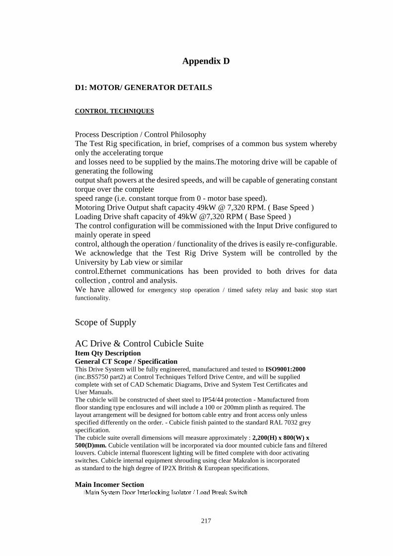
217
Appendix D
D1: MOTOR/ GENERATOR DETAILS
CONTROL TECHNIQUES
Process Description / Control Philosophy
The Test Rig specification, in brief, comprises of a common bus system whereby
only the accelerating torque
and losses need to be supplied by the mains.The motoring drive will be capable of
generating the following
output shaft powers at the desired speeds, and will be capable of generating constant
torque over the complete
speed range (i.e. constant torque from 0 - motor base speed).
Motoring Drive Output shaft capacity 49kW @ 7,320 RPM. ( Base Speed )
Loading Drive shaft capacity of 49kW @7,320 RPM ( Base Speed )
The control configuration will be commissioned with the Input Drive configured to
mainly operate in speed
control, although the operation / functionality of the drives is easily re-configurable.
We acknowledge that the Test Rig Drive System will be controlled by the
University by Lab view or similar
control.Ethernet communications has been provided to both drives for data
collection , control and analysis.
We have allowed for emergency stop operation / timed safety relay and basic stop start
functionality.
Scope of Supply
AC Drive & Control Cubicle Suite Item Qty Description
General CT Scope / Specification This Drive System will be fully engineered, manufactured and tested to ISO9001:2000
(inc.BS5750 part2) at Control Techniques Telford Drive Centre, and will be supplied
complete with set of CAD Schematic Diagrams, Drive and System Test Certificates and
User Manuals.
The cubicle will be constructed of sheet steel to IP54/44 protection - Manufactured from
floor standing type enclosures and will include a 100 or 200mm plinth as required. The
layout arrangement will be designed for bottom cable entry and front access only unless
specified differently on the order. - Cubicle finish painted to the standard RAL 7032 grey
specification.
The cubicle suite overall dimensions will measure approximately : 2,200(H) x 800(W) x
500(D)mm. Cubicle ventilation will be incorporated via door mounted cubicle fans and filtered
louvers. Cubicle internal fluorescent lighting will be fitted complete with door activating
switches. Cubicle internal equipment shrouding using clear Makralon is incorporated
as standard to the high degree of IP2X British & European specifications.
Main Incomer Section
218
– SP4403 Motoring Drive
– SP4403 Loading Drive
es ( x2 )
-Stop fail safe module
es as standard
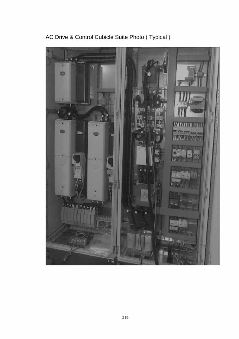
219
AC Drive & Control Cubicle Suite Photo ( Typical )
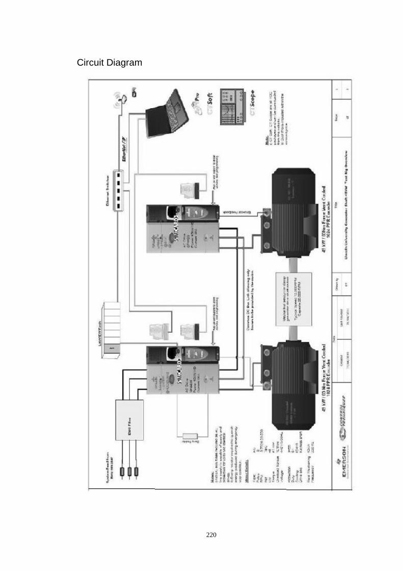
220
Circuit Diagram

221
AC Motor Details
Based on the supply of 2 off Oswald QDi13 2-2Fi
Type QDi13 2 2
Voltage 440 Volt
FLC 77A
Base Speed 7,320 RPM
Max Speed 20,000 RPM
Power 49kW
Frequency 123/326 Hz
Poles 2
IP Rating 23
Bearings Insulated
Encoder Heidenhaim 512 PPR TTL 5 V Quadrature
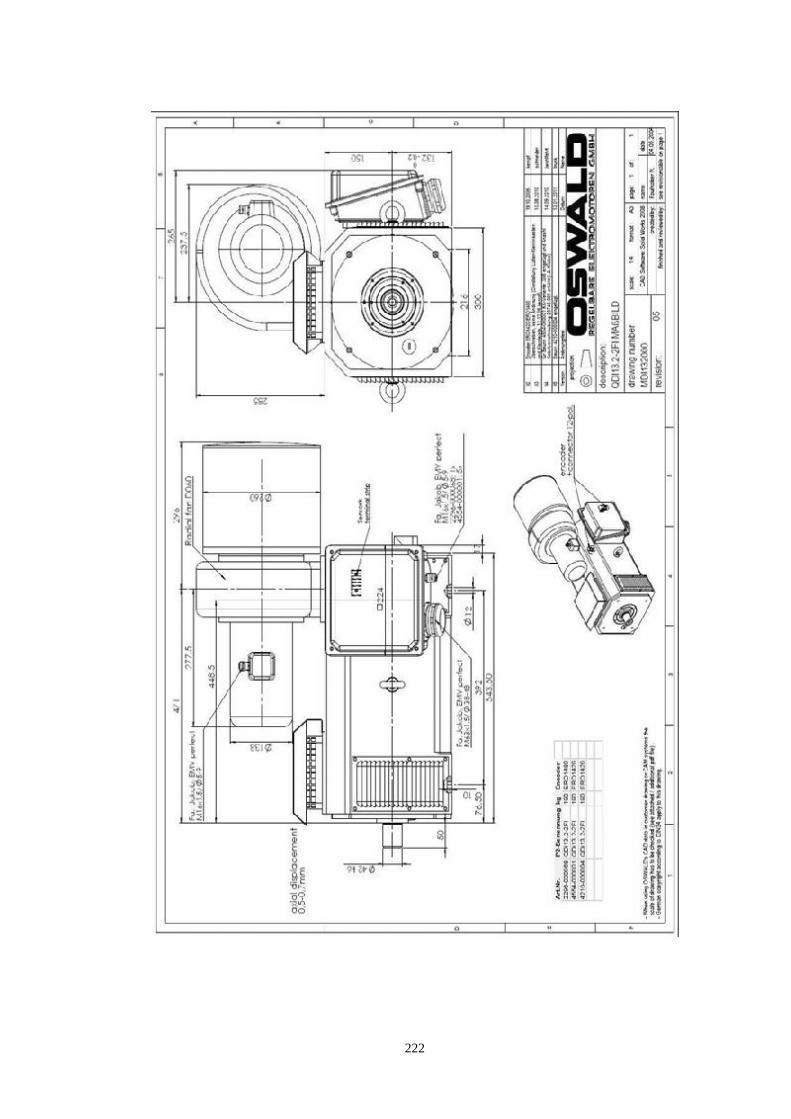
222
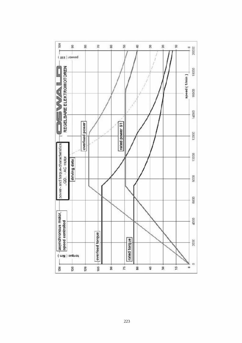
223
224
D2: LASER MEASUREMENT DETAILS
MICRO-EPSILON
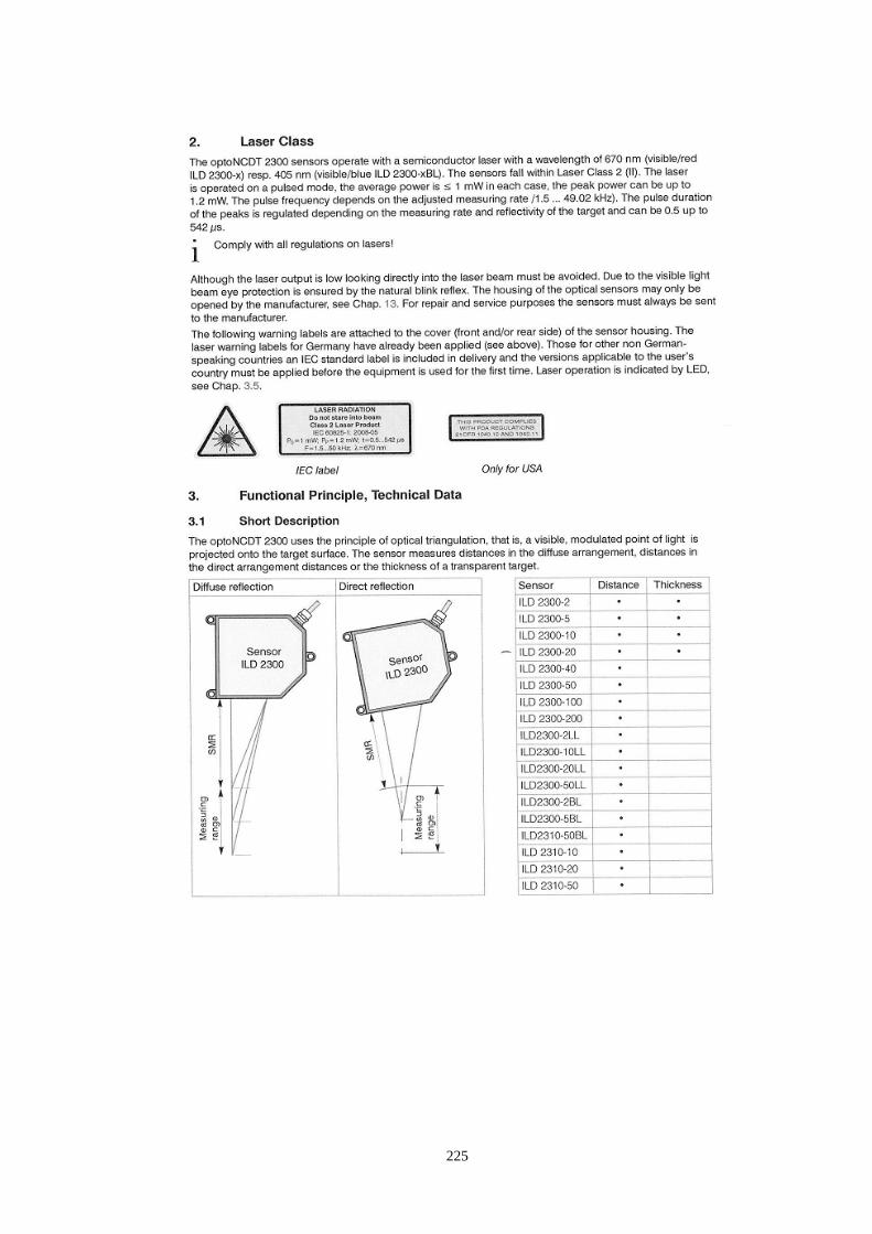
225
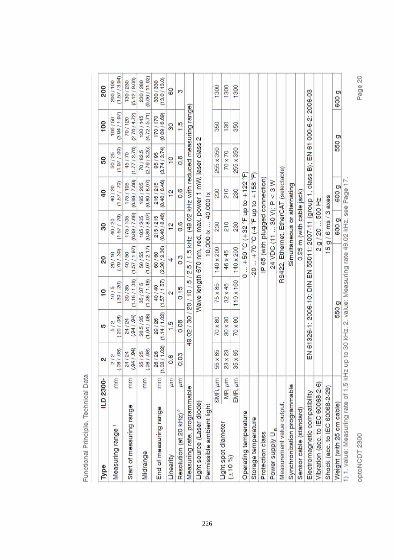
226
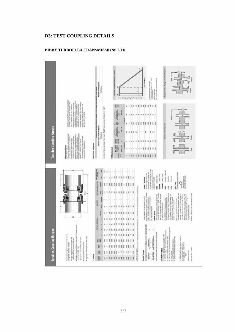
227
D3: TEST COUPLING DETAILS
BIBBY TURBOFLEX TRANSMISSIONS LTD
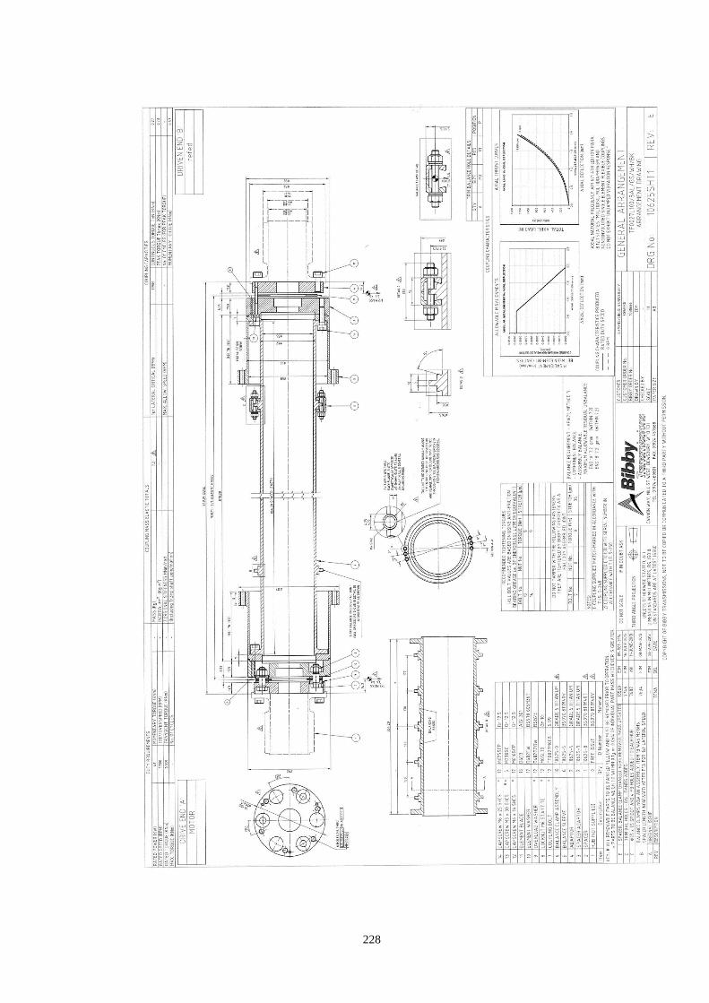
228