Embed Size (px)
Citation preview
ANALYSIS �� Moody’s Analytics Case-Shiller Home Price Index Forecast Methodology
January 2015
Moody’s Analytics Case-Shiller Home Price Index Forecast Methodology
Prepared byCelia [email protected] Director Andres [email protected] Director
Contact UsEmail [email protected]
U.S./Canada +1.866.275.3266
EMEA (London) +44.20.7772.5454 (Prague) +420.224.222.929
Asia/Pacific +852.3551.3077
All Others +1.610.235.5299
Web www.economy.com
Abstract
Moody’s Analytics has developed a combined econometric model for the Federal Housing Finance Agency house price indexes and the CoreLogic Case-Shiller home price indexes. The econometric model uses the relationship between the Case-Shiller house price and the FHFA house price indexes in national, state and metropolitan area housing markets. The economic and demographic forces that drive house price determination will mostly impact Case-Shiller prices through the FHFA indexes. The model that Moody’s Analytics has developed is a tool for forecasting the Case-Shiller Home Price Index, with the ability to generate alternative forecast scenarios such as the Federal Reserve Bank’s Comprehensive Capital Analysis and Review scenarios.
eConomiC & Consumer Credit AnAlytiCs
MOODY’S ANALYTICS / Copyright© 2015 1
ANALYSIS ��
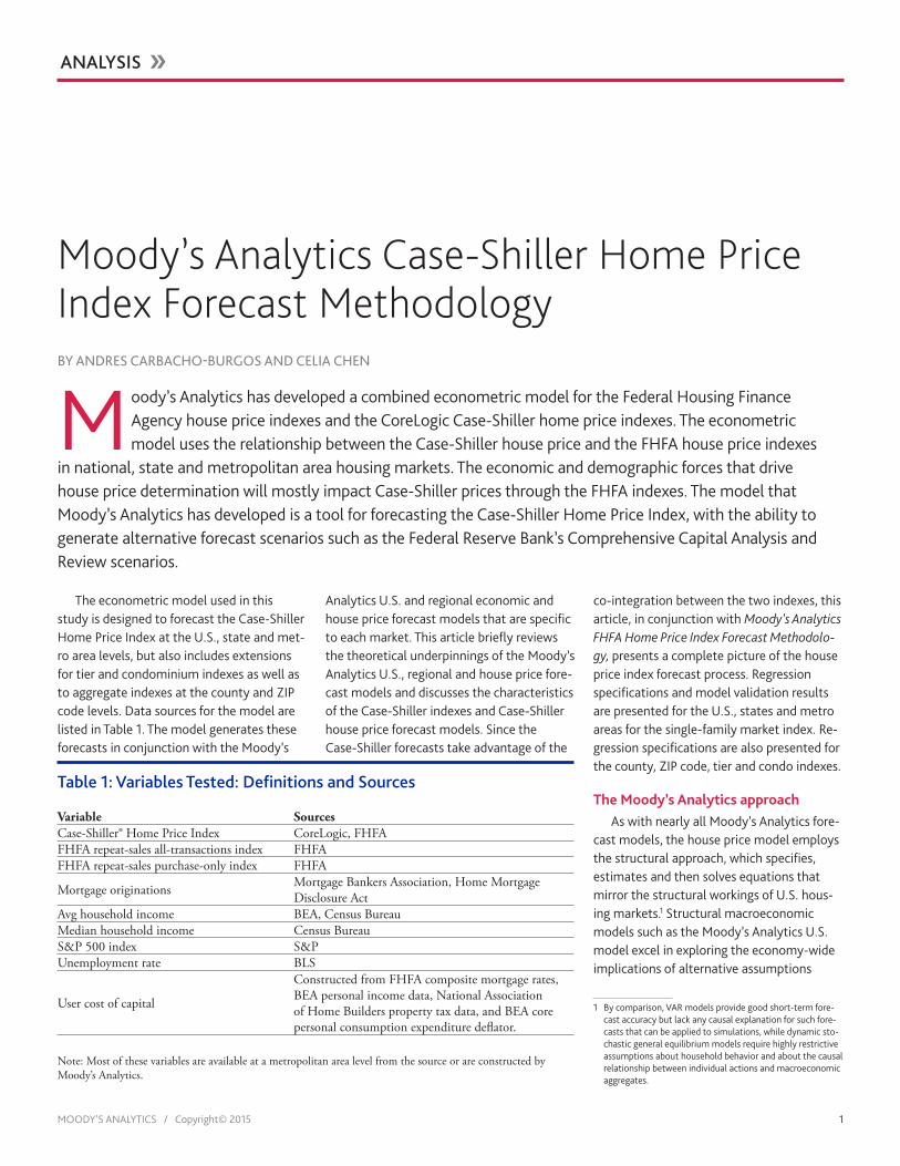
Moody’s Analytics Case-Shiller Home Price Index Forecast MethodologyBy AnDrES CArBAChO-BUrgOS AnD CELiA ChEn
Moody’s Analytics has developed a combined econometric model for the Federal Housing Finance Agency house price indexes and the CoreLogic Case-Shiller home price indexes. The econometric model uses the relationship between the Case-Shiller house price and the FHFA house price indexes
in national, state and metropolitan area housing markets. The economic and demographic forces that drive house price determination will mostly impact Case-Shiller prices through the FHFA indexes. The model that Moody’s Analytics has developed is a tool for forecasting the Case-Shiller Home Price Index, with the ability to generate alternative forecast scenarios such as the Federal Reserve Bank’s Comprehensive Capital Analysis and Review scenarios.
The econometric model used in this study is designed to forecast the Case-Shiller Home Price Index at the U.S., state and met-ro area levels, but also includes extensions for tier and condominium indexes as well as to aggregate indexes at the county and ZIP code levels. Data sources for the model are listed in Table 1. The model generates these forecasts in conjunction with the Moody’s
Analytics U.S. and regional economic and house price forecast models that are specific to each market. This article briefly reviews the theoretical underpinnings of the Moody’s Analytics U.S., regional and house price fore-cast models and discusses the characteristics of the Case-Shiller indexes and Case-Shiller house price forecast models. Since the Case-Shiller forecasts take advantage of the
co-integration between the two indexes, this article, in conjunction with Moody’s Analytics FHFA Home Price Index Forecast Methodolo-gy, presents a complete picture of the house price index forecast process. Regression specifications and model validation results are presented for the U.S., states and metro areas for the single-family market index. Re-gression specifications are also presented for the county, ZIP code, tier and condo indexes.
the moody’s Analytics approachAs with nearly all Moody’s Analytics fore-
cast models, the house price model employs the structural approach, which specifies, estimates and then solves equations that mirror the structural workings of U.S. hous-ing markets.1 Structural macroeconomic models such as the Moody’s Analytics U.S. model excel in exploring the economy-wide implications of alternative assumptions
1 By comparison, VAR models provide good short-term fore-cast accuracy but lack any causal explanation for such fore-casts that can be applied to simulations, while dynamic sto-chastic general equilibrium models require highly restrictive assumptions about household behavior and about the causal relationship between individual actions and macroeconomic aggregates.
Table 1: Variables Tested: Definitions and Sources
Variable SourcesCase-Shiller® Home Price Index CoreLogic, FHFAFHFA repeat-sales all-transactions index FHFAFHFA repeat-sales purchase-only index FHFA
Mortgage originations Mortgage Bankers Association, Home Mortgage Disclosure Act
Avg household income BEA, Census BureauMedian household income Census BureauS&P 500 index S&PUnemployment rate BLS
User cost of capital
Constructed from FHFA composite mortgage rates, BEA personal income data, National Association of Home Builders property tax data, and BEA core personal consumption expenditure deflator.
Note: Most of these variables are available at a metropolitan area level from the source or are constructed by Moody’s Analytics.
MOODY’S ANALYTICS / Copyright© 2015 2
ANALYSIS �� Moody’s Analytics Case-Shiller Home Price Index Forecast Methodology
about the future, including those used in stress-testing exercises. This approach is also well-suited to extrapolating implications for specific regions.
House price determinationThe approach to model house price de-
termination for the Case-Shiller index is a variant of the structural model, leveraging from the Moody’s Analytics model of the FHFA’s repeat-purchase house price index. This approach ties the Case-Shiller house price forecasts to their fundamental eco-nomic drivers while utilizing the complete state and metro area coverage available in the FHFA index to generate a good relation-ship between the economic variables and house prices.2 It also ensures consistency across the suite of house price indexes fore-cast by Moody’s Analytics.
The FHFA house price forecast forms the backbone for house price determina-tion. This fully specified structural model of housing demand and supply allows for serial correlation and mean reversion in regional housing markets. This model can identify the forces driving house prices and assess the degree to which house prices can be explained by fundamental, persistent trends and the degree to which they are explained by more temporal, business cycle-related
2 For these house price forecast models, Moody’s Analytics uses the 2000 OMB metro definitions, as some key data sources such as the Bureau of Labor Statistics have not yet switched to the 2010 OMB definitions. Also, metropolitan divisions are treated identically to metropolitan statistical areas; both are referred to as “metro areas.” MSAs that are divided into metro divisions are not considered.
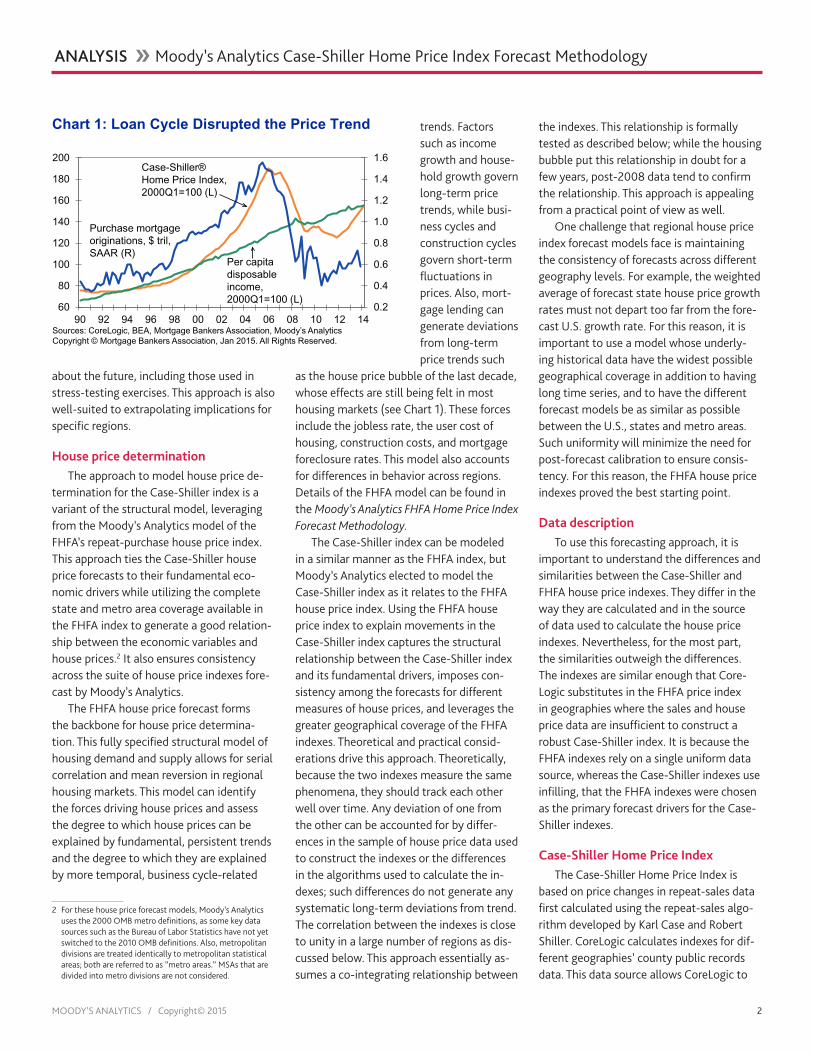
trends. Factors such as income growth and house-hold growth govern long-term price trends, while busi-ness cycles and construction cycles govern short-term fluctuations in prices. Also, mort-gage lending can generate deviations from long-term price trends such
as the house price bubble of the last decade, whose effects are still being felt in most housing markets (see Chart 1). These forces include the jobless rate, the user cost of housing, construction costs, and mortgage foreclosure rates. This model also accounts for differences in behavior across regions. Details of the FHFA model can be found in the Moody’s Analytics FHFA Home Price Index Forecast Methodology.
The Case-Shiller index can be modeled in a similar manner as the FHFA index, but Moody’s Analytics elected to model the Case-Shiller index as it relates to the FHFA house price index. Using the FHFA house price index to explain movements in the Case-Shiller index captures the structural relationship between the Case-Shiller index and its fundamental drivers, imposes con-sistency among the forecasts for different measures of house prices, and leverages the greater geographical coverage of the FHFA indexes. Theoretical and practical consid-erations drive this approach. Theoretically, because the two indexes measure the same phenomena, they should track each other well over time. Any deviation of one from the other can be accounted for by differ-ences in the sample of house price data used to construct the indexes or the differences in the algorithms used to calculate the in-dexes; such differences do not generate any systematic long-term deviations from trend. The correlation between the indexes is close to unity in a large number of regions as dis-cussed below. This approach essentially as-sumes a co-integrating relationship between
the indexes. This relationship is formally tested as described below; while the housing bubble put this relationship in doubt for a few years, post-2008 data tend to confirm the relationship. This approach is appealing from a practical point of view as well.
One challenge that regional house price index forecast models face is maintaining the consistency of forecasts across different geography levels. For example, the weighted average of forecast state house price growth rates must not depart too far from the fore-cast U.S. growth rate. For this reason, it is important to use a model whose underly-ing historical data have the widest possible geographical coverage in addition to having long time series, and to have the different forecast models be as similar as possible between the U.S., states and metro areas. Such uniformity will minimize the need for post-forecast calibration to ensure consis-tency. For this reason, the FHFA house price indexes proved the best starting point.
data descriptionTo use this forecasting approach, it is
important to understand the differences and similarities between the Case-Shiller and FHFA house price indexes. They differ in the way they are calculated and in the source of data used to calculate the house price indexes. Nevertheless, for the most part, the similarities outweigh the differences. The indexes are similar enough that Core-Logic substitutes in the FHFA price index in geographies where the sales and house price data are insufficient to construct a robust Case-Shiller index. It is because the FHFA indexes rely on a single uniform data source, whereas the Case-Shiller indexes use infilling, that the FHFA indexes were chosen as the primary forecast drivers for the Case-Shiller indexes.
Case-shiller Home Price indexThe Case-Shiller Home Price Index is
based on price changes in repeat-sales data first calculated using the repeat-sales algo-rithm developed by Karl Case and Robert Shiller. CoreLogic calculates indexes for dif-ferent geographies’ county public records data. This data source allows CoreLogic to
11
0.2
0.4
0.6
0.8
1.0
1.2
1.4
1.6
60
80
100
120
140
160
180
200
90 92 94 96 98 00 02 04 06 08 10 12 14
Chart 1: Loan Cycle Disrupted the Price Trend
Sources: CoreLogic, BEA, Mortgage Bankers Association, Moody’s AnalyticsCopyright © Mortgage Bankers Association, Jan 2015. All Rights Reserved.
Purchase mortgage originations, $ tril, SAAR (R)
Per capita disposable income, 2000Q1=100 (L)
Case-Shiller® Home Price Index, 2000Q1=100 (L)
MOODY’S ANALYTICS / Copyright© 2015 3
ANALYSIS �� Moody’s Analytics Case-Shiller Home Price Index Forecast Methodology
generate Case-Shiller indexes for all states that do not have nondisclosure laws and for most of the metro areas therein. In some cases, especially for small metro areas, the data are not sufficient to generate stable Case-Shiller indexes. For such metro areas, CoreLogic fills in the Case-Shiller indexes with rebased FHFA indexes.
Many states have nondisclosure laws that prevent county offices from releasing sales price data. These states are Alabama, Alaska, Idaho, Indiana, Kansas, Louisiana, Maine, Mississippi, Missouri, Montana, New Mexico, North Dakota, Texas, Utah and Wyoming. For these states and the metro areas within them, CoreLogic also fills in Case-Shiller in-dexes with rebased FHFA indexes.3
All told, CoreLogic covers 216 metro areas and 36 states with CoreLogic indexes gener-ated with its own data, while the remaining states and metro areas use rebased FHFA indexes. In the models that follow, Moody’s Analytics uses regressions to forecast only these states and metro areas with indepen-dent CoreLogic data. The Case-Shiller index forecasts for the remaining 15 nondisclosure states and the remaining 168 metro areas are obtained simply by growing out the rebased historical FHFA indexes with the growth rates of the corresponding FHFA index forecasts.
FHFA house price indexesThe Federal Housing Finance Agency
Home Price Index also uses the repeat-sales algorithm created by Case-Shiller; the main difference between the two indexes is thus not on the methodology but in the data sources.4 The data used to construct the purchase-only and all-transaction FHFA house price indexes are similar to those used to calculate the Case-Shiller HPI, but there are some key differences. The FHFA bases
3 CoreLogic uses FHFA purchase-only indexes to fill in for Case-Shiller if these are available; otherwise, it uses FHFA all-transactions indexes, which include refinancing appraisal values in addition to purchase transactions.
4 The one exception to this methodological similarity is that Case-Shiller indexes calculated with CoreLogic data are value-weighted, whereas FHFA indexes are unit-weighted. In theory, this can lead the Case-Shiller indexes to have larger deviations over time than FHFA indexes calculated with the same data, but the extent of this difference is difficult to measure.
its HPI on price data from repeat mortgage transactions on single-family properties whose mortgages have been purchased or securitized by Fannie Mae and Freddie Mac. The HPI is updated monthly for the U.S. and census divisions and on a quarterly basis for states and metro areas, incorporating ad-ditional data as mortgages are purchased or securitized by Fannie and Freddie. These source data are limited to loans that are both conforming and conventional, as described below:
Conforming loan types » Government-sponsored enterprise
(Fannie Mae and Freddie Mac) loans that follow their guidelines
» Federal Housing Administration (FHA) loans that insure first mortgages
» Veterans Affairs (VA) and Rural Hous-ing Service (RHS) insured loans from banks or other lenders
Conventional loans » Any loan not under a government-
insured program
Because Fannie Mae and Freddie Mac can purchase only mortgages that are conform-ing and conventional, several types of home purchase transactions are excluded from the FHFA data. These include jumbo mortgages that exceed conforming loan limits, agency mortgages from the FHA, VA and RHS, and of course purchases that are financed with cash or nonmortgage lending. Also, during the height of the housing bubble a substan-tial share of mortgages were conforming and conventional but were bought up by private-label companies rather than by Fannie Mae and Freddie Mac, and would thus not have been included in the data used to calculate FHFA indexes. Because of this narrower base of data, the FHFA indexes provide a more limited look at house price transactions than do the Case-Shiller indexes, but their larger metro area coverage compensates for this disadvantage.
The FHFA reports two price indexes, a purchase-only index and an all-transaction index. The purchase index includes only house price data from purchase mortgages,
while the all-transaction index includes house price data from mortgages for pur-chase and home value appraisals for refi-nancing mortgages. Since it represents true market prices better, the purchase-only index is the preferable measure, but data limitations make it available only for the states and larger metro areas. The FHFA publishes purchase-only indexes for the U.S., all 50 states, Washington DC, and 100 metro areas.
Comparing Case-shiller and FHFABecause the Case-Shiller index includes
information for all arm’s-length home sales in regions where it is available regardless of the source of financing, it better represents house price trends for the entire housing market. There is one important exception: the Case-Shiller indexes exclude sales pairs that span bank repossessions (which are considered non-arm’s length transactions), in effect excluding most real estate-owned sales. By comparison, the FHFA indexes can include REO sales, but this greater inclusiv-ity is offset by their lack of cash, jumbo mortgage, and private label transactions; as a result, the difference in the cyclical swings for the two indexes is not large. In the long run, the two indexes trend together well, but short-run cyclical differences are evident and are related to the different types of data used to calculate the indexes.
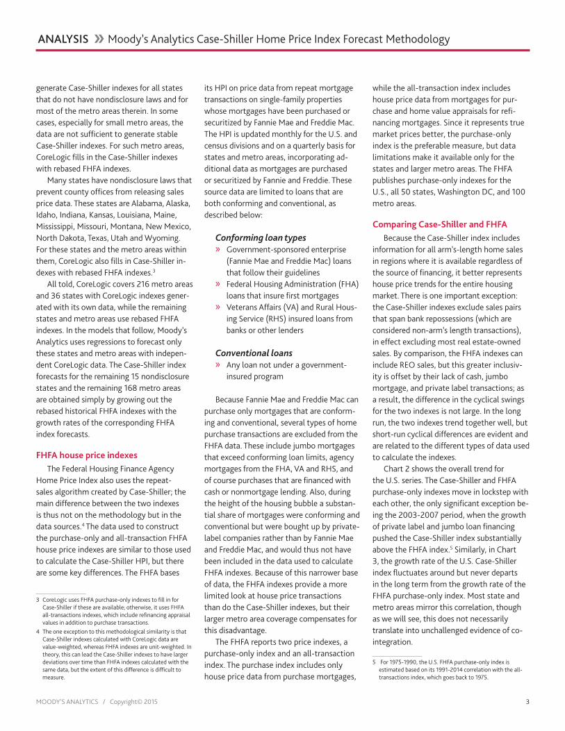
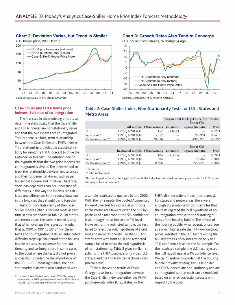
Chart 2 shows the overall trend for the U.S. series. The Case-Shiller and FHFA purchase-only indexes move in lockstep with each other, the only significant exception be-ing the 2003-2007 period, when the growth of private label and jumbo loan financing pushed the Case-Shiller index substantially above the FHFA index.5 Similarly, in Chart 3, the growth rate of the U.S. Case-Shiller index fluctuates around but never departs in the long term from the growth rate of the FHFA purchase-only index. Most state and metro areas mirror this correlation, though as we will see, this does not necessarily translate into unchallenged evidence of co-integration.
5 For 1975-1990, the U.S. FHFA purchase-only index is estimated based on its 1991-2014 correlation with the all-transactions index, which goes back to 1975.
MOODY’S ANALYTICS / Copyright© 2015 4
ANALYSIS �� Moody’s Analytics Case-Shiller Home Price Index Forecast Methodology
Case-shiller and FHFA home price indexes: evidence of co-integration
The first step in the modeling effort is to determine statistically that the Case-Shiller and FHFA indexes are non-stationary series and that the two indexes are co-integrated. That is, there is a long-term relationship between the Case-Shiller and FHFA indexes. This relationship provides the statistical va-lidity for using the FHFA forecast to drive the Case-Shiller forecast. The intuition behind the hypothesis that the two price indexes are co-integrated is simple. The indexes tend to track the relationship between house prices and their fundamental drivers such as per household income and inflation. Therefore, short-run departures can occur because of differences in the way the indexes are calcu-lated and differences in the source data, but in the long run, they should trend together.
Tests for non-stationarity of the Case-Shiller indexes (that is, for unit roots in each time series) are shown in Table 2. For states and metro areas, the sample tested is only that which overlaps the regression model, that is, 1990 or 1991 to 2013.6 For these tests and co-integration tests, an anticipated difficulty crops up: The period of the housing bubble reduces the evidence for non-sta-tionarity and co-integration, in some cases to the point where the tests did not prove successful. To underline the importance of the 2002-2008 housing bubble, the non-stationarity tests were also conducted with
6 For the U.S. test, the test period was 1975-2014, using an estimate of the FHFA purchase-only index for 1975-1990, as the 1991-2014 sample period has too few observations.
a sample restricted to quarters before 2002. With the full sample, the pooled Augmented Dickey-Fuller test for individual unit roots at the metro area level rejected the null hy-pothesis of a unit root at the 5% confidence level, though not as low as the 1% level. However, for the restricted sample, the test failed to reject the null hypothesis of a unit root and non-stationarity. For the U.S. and states, tests with both a full and restricted sample failed to reject the null hypothesis of non-stationarity. Table 3 gives similar re-sults for the FHFA purchase-only index (U.S., states), and the FHFA all-transactions index (metro areas).
Table 4 shows the results of Engle-Granger tests for co-integration between the Case-Shiller index and either the FHFA purchase-only index (U.S., states) or the
FHFA all-transactions index (metro areas). For states and metro areas, there were enough observations for both samples that the tests rejected the null hypothesis of no co-integration even with the distorting ef-fects of the housing bubble. The effects of the housing bubble, when overall prices rose at a much higher rate than FHFA-monitored prices, resulted in the U.S. test rejecting the null hypothesis of co-integration only at a 10% confidence level for the full sample. For the restricted sample, the U.S. test rejected the null hypothesis at a 1% confidence level. We can therefore conclude that the housing bubble notwithstanding, the Case-Shiller and FHFA indexes are non-stationary and are co-integrated, so that each can be modeled based on an error correction process with respect to the other.
33
-20
-15
-10
-5
0
5
10
15
20
76 79 82 85 88 91 94 97 00 03 06 09 12
FHFA purchase-only (estimate)FHFA purchase-only (actual)Case-Shiller® Home Price Index
Chart 3: Growth Rates Also Tend to ConvergeU.S. house price indexes, % change yr ago
Sources: CoreLogic, FHFA, Moody’s Analytics
22
0
40
80
120
160
200
75 78 81 84 87 90 93 96 99 02 05 08 11 14
FHFA purchase-only (estimate)FHFA purchase-only (actual)Case-Shiller® House Price Index
Chart 2: Deviation Varies, but Trend Is SimilarU.S. house price, 2000Q1=100
Sources: CoreLogic, FHFA, Moody’s Analytics
Table 2: Case-Shiller Index, Non-Stationarity Tests for U.S., States and Metro Areas
Augmented Dickey-Fuller Test Results
Full sample Observations t-statisticFisher Chi-
square Statistic Prob.U.S. 1975Q1-2014Q1 157 -1.0823 -- 0.7221State pool * 1991Q1-2013Q4 3,312 -- 70.0951 0.5416Metro area pool ** 1990Q1-2013Q4 20,736 -- 490.6920 0.0265
Restricted sample Observations t-statisticFisher Chi-
square Statistic Prob.U.S. 1975Q1-2001Q4 104 -1.3704 -- 0.5941State pool * 1991Q1-2001Q4 1,584 -- 19.8467 1.0000Metro area pool ** 1990Q1-2001Q4 10,368 -- 255.9540 1.0000
* 36 states** 216 metro areasThe null hypothesis is that the log of the Case-Shiller index has individual unit root processes for the U.S., or for the geographies in each pool.
MOODY’S ANALYTICS / Copyright© 2015 5
ANALYSIS �� Moody’s Analytics Case-Shiller Home Price Index Forecast Methodology
Case-shiller HPi models: u.s. and states
Once the Case-Shiller and FHFA home price indexes are determined to be co-integrated, Moody’s Analytics turns to the models that best explain variations in the Case-Shiller index relative to the FHFA index and other drivers that would explain the short-run variations between the indexes.7 The models tested are error correction models that allow for near-term
7 For modeling purposes, the Case-Shiller and FHFA indexes are benchmarked to their own values from the first quarter of 2000 in order to minimize comparability problems. Both indexes are seasonally adjusted and are updated quarterly for FHFA indexes and monthly for the Case-Shiller indexes, though the regression model is quarterly.
differences between the Case-Shiller and FHFA indexes while ensuring that long-term trends are similar. The model drives convergence of the Case-Shiller index to the FHFA index through a mean reversion term, where the mean is effectively the FHFA index forecast. These models can be expressed as follows:
Δlog(𝐶𝐶𝐶𝐶𝐶𝐶𝑡𝑡) = 𝛽𝛽1Δlog(𝐶𝐶𝐶𝐶𝐶𝐶𝑡𝑡−1)+ 𝛽𝛽2Δ log(𝐹𝐹𝐹𝐹𝐹𝐹𝐹𝐹𝑡𝑡)+ 𝛽𝛽3(log(𝐶𝐶𝐶𝐶𝐶𝐶𝑡𝑡−1) − log(𝐹𝐹𝐹𝐹𝐹𝐹𝐹𝐹𝑡𝑡−1))+ 𝛽𝛽4𝑋𝑋 + 𝜇𝜇𝑡𝑡
Where:
» CSI = Case-Shiller index for region,
» FHFA = FHFA purchase-only index for U.S. and states, or all-transactions in-dex for metro areas,
» X = variables that can explain short-term differences between behavior of the CSI and FHFA indexes.
» μ is the random error term. » Subscript t indicates the current quar-
ter and t-1 the previous quarter.
The error correction term with the co-efficient β3 drives the Case-Shiller index to appreciate more quickly (slowly) when the Case-Shiller index has been appreciat-ing more slowly (quickly) than the FHFA index.8 The Case-Shiller index is also driv-en by how quickly the FHFA index appre-ciates; hence this equation includes the contemporaneous FHFA index. Note that this term captures concurrent economic and demographic drivers of house prices. The faster the FHFA index appreciates, the faster the Case-Shiller index appreciates.
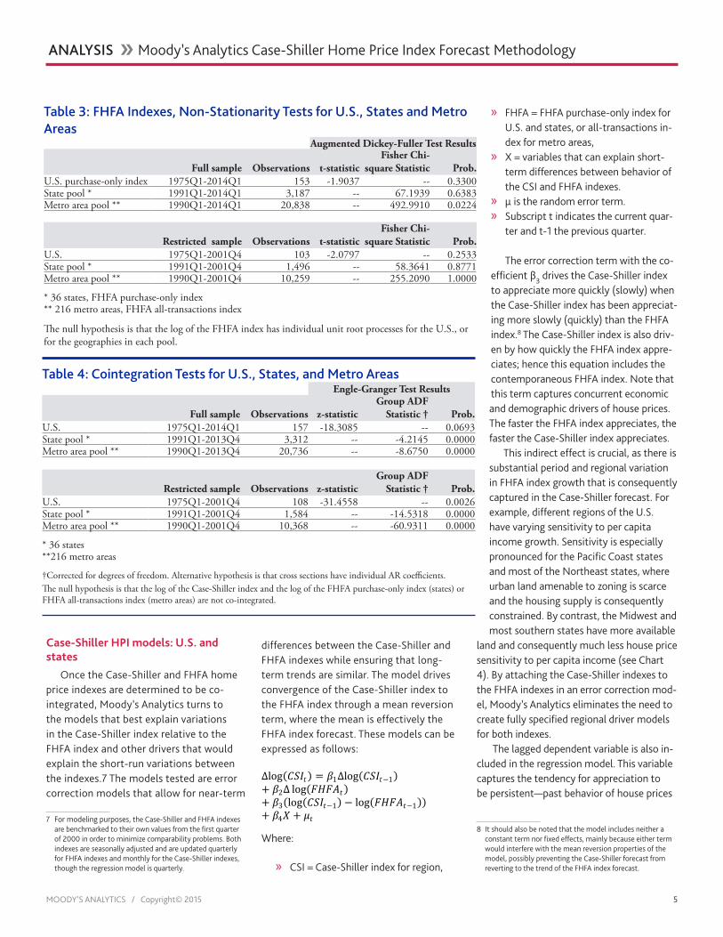
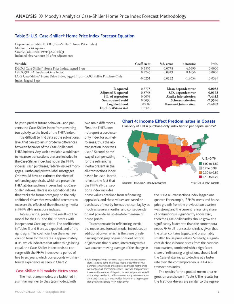
This indirect effect is crucial, as there is substantial period and regional variation in FHFA index growth that is consequently captured in the Case-Shiller forecast. For example, different regions of the U.S. have varying sensitivity to per capita income growth. Sensitivity is especially pronounced for the Pacific Coast states and most of the Northeast states, where urban land amenable to zoning is scarce and the housing supply is consequently constrained. By contrast, the Midwest and most southern states have more available
land and consequently much less house price sensitivity to per capita income (see Chart 4). By attaching the Case-Shiller indexes to the FHFA indexes in an error correction mod-el, Moody’s Analytics eliminates the need to create fully specified regional driver models for both indexes.
The lagged dependent variable is also in-cluded in the regression model. This variable captures the tendency for appreciation to be persistent—past behavior of house prices
8 It should also be noted that the model includes neither a constant term nor fixed effects, mainly because either term would interfere with the mean reversion properties of the model, possibly preventing the Case-Shiller forecast from reverting to the trend of the FHFA index forecast.
Table 3: FHFA Indexes, Non-Stationarity Tests for U.S., States and Metro Areas
Augmented Dickey-Fuller Test Results
Full sample Observations t-statisticFisher Chi-
square Statistic Prob.U.S. purchase-only index 1975Q1-2014Q1 153 -1.9037 -- 0.3300State pool * 1991Q1-2014Q1 3,187 -- 67.1939 0.6383Metro area pool ** 1990Q1-2014Q1 20,838 -- 492.9910 0.0224
Restricted sample Observations t-statisticFisher Chi-
square Statistic Prob.U.S. 1975Q1-2001Q4 103 -2.0797 -- 0.2533State pool * 1991Q1-2001Q4 1,496 -- 58.3641 0.8771Metro area pool ** 1990Q1-2001Q4 10,259 -- 255.2090 1.0000
* 36 states, FHFA purchase-only index** 216 metro areas, FHFA all-transactions index
The null hypothesis is that the log of the FHFA index has individual unit root processes for the U.S., or for the geographies in each pool.
Table 4: Cointegration Tests for U.S., States, and Metro AreasEngle-Granger Test Results
Full sample Observations z-statisticGroup ADF
Statistic † Prob.U.S. 1975Q1-2014Q1 157 -18.3085 -- 0.0693State pool * 1991Q1-2013Q4 3,312 -- -4.2145 0.0000Metro area pool ** 1990Q1-2013Q4 20,736 -- -8.6750 0.0000
Restricted sample Observations z-statisticGroup ADF
Statistic † Prob.U.S. 1975Q1-2001Q4 108 -31.4558 -- 0.0026State pool * 1991Q1-2001Q4 1,584 -- -14.5318 0.0000Metro area pool ** 1990Q1-2001Q4 10,368 -- -60.9311 0.0000
* 36 states**216 metro areas
†Corrected for degrees of freedom. Alternative hypothesis is that cross sections have individual AR coefficients.The null hypothesis is that the log of the Case-Shiller index and the log of the FHFA purchase-only index (states) or FHFA all-transactions index (metro areas) are not co-integrated.
MOODY’S ANALYTICS / Copyright© 2015 6
ANALYSIS �� Moody’s Analytics Case-Shiller Home Price Index Forecast Methodology
helps to predict future behavior—and pre-vents the Case-Shiller index from reverting too quickly to the level of the FHFA index.
It is difficult to find data at the subnational level that can explain short-term differences between behavior of the Case-Shiller and FHFA indexes. Any such a variable would have to measure transactions that are included in the Case-Shiller index but not in the FHFA indexes: cash purchases, federal-insured mort-gages, jumbo and private-label mortgages. Or it would have to estimate the effect of refinancing appraisals, which are present in FHFA all-transactions indexes but not Case-Shiller indexes. There is no subnational data that tracks the former category, so the only additional driver that was added attempts to measure the effects of the refinancing inertia in FHFA all-transactions indexes.
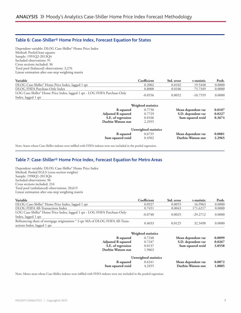
Tables 5 and 6 present the results of the model for the U.S. and the 36 states with independent CoreLogic data. The coefficients in Tables 5 and 6 are as expected, and of the right signs. The coefficient on the mean re-version term for the states is approximately 0.05, which indicates that other things being equal, the Case-Shiller index tends to con-verge with the FHFA index over a period of five to six years, which corresponds with his-torical experience as seen in Chart 2.
Case-shiller HPi models: metro areasThe metro area models are fashioned in
a similar manner to the state models, with
two main differences. First, the FHFA does not report a purchase-only index for all met-ro areas, thus the all-transaction index was used.9 Second, some way of compensating for the refinancing inertia present in the all-transactions index has to be used. Inertia refers to the fact that the FHFA all-transac-tions index includes home values obtained from refinancing appraisals, and these values are based on purchases of nearby homes that can lag by as much as several months, and consequently do not provide an up-to-date measure of house prices.
To compensate for refinancing inertia, the metro area forecast model introduces an additional driver, which is the share of refi-nancing mortgage originations out of total originations that quarter, interacting with a two-quarter moving average of the change in
9 It is also possible to have two separate metro area regres-sions, splitting pools into those metro areas where FHFA purchase-only indexes are available and those metro areas with only an all-transactions index. However, this procedure increases the number of steps in the forecast process as well as the steps needed to calibrate consistency between metro areas and states, so it was avoided in favor of a single regres-sion pool with a single FHFA index driver.
the FHFA all-transactions index lagged one quarter. For example, if FHFA-measured house price growth from the previous two quarters was strong and the current refinancing share of originations is significantly above zero, then the Case-Shiller index should grow at a significantly faster rate than the contempora-neous FHFA all-transactions index, given that the latter contains lagged, and presumably smaller, house price values. Similarly, a signifi-cant decline in house prices from the previous two quarters, combined with a significant share of refinancing originations, should lead the Case-Shiller index to decline at a faster rate than the contemporaneous FHFA all-transactions index.
The results for the pooled metro area re-gression are shown in Table 7. The results for the first four drivers are similar to the regres-
44
Chart 4: Income Effect Predominates in Coasts Elasticity of FHFA purchase-only index tied to per capita income*
Sources: FHFA, BEA, Moody’s Analytics *1991Q1-2014Q1 sample
1.00 to 1.82
0.7 to 0.99
0.30 to 0.69
0.10 to 0.29
U.S.=0.76
Table 5: U.S. Case-Shiller® Home Price Index Forecast Equation
Dependent variable: DLOG(Case-Shiller® House Price Index)Method: Least squaresSample (adjusted): 1991Q2-2014Q1Included observations: 92 after adjustments
Variable Coefficient Std. error t-statistic Prob. DLOG Case-Shiller® Home Price Index, lagged 1 qtr 0.3555 0.0778 4.5690 0.0000DLOG(FHFA Purchase-Only Index) 0.7745 0.0949 8.1656 0.0000LOG Case-Shiller® Home Price Index, lagged 1 qtr - LOG FHFA Purchase-Only Index, lagged 1 qtr -0.0251 0.0132 -1.9054 0.0599
R-squared 0.8775 Mean dependent var 0.0083Adjusted R-squared 0.8748 S.D. dependent var 0.0163
S.E. of regression 0.0058 Akaike info criterion -7.4413Sum squared resid 0.0030 Schwarz criterion -7.3596
Log likelihood 349.02 Hannan-Quinn criter. -7.4083Durbin-Watson stat 1.8320
MOODY’S ANALYTICS / Copyright© 2015 7
ANALYSIS �� Moody’s Analytics Case-Shiller Home Price Index Forecast Methodology
Table 6: Case-Shiller® Home Price Index, Forecast Equation for States
Dependent variable: DLOG Case-Shiller® Home Price IndexMethod: Pooled least squaresSample: 1991Q2-2013Q4Included observations: 91Cross sections included: 36Total pool (balanced) observations: 3,276Linear estimation after one-step weighting matrix
Variable Coefficient Std. error t-statistic Prob. DLOG Case-Shiller® Home Price Index, lagged 1 qtr 0.2002 0.0102 19.5448 0.0000DLOG FHFA Purchase-Only Index 0.8000 0.0106 75.7349 0.0000LOG Case-Shiller® Home Price Index, lagged 1 qtr - LOG FHFA Purchase-Only Index, lagged 1 qtr -0.0556 0.0052 -10.7559 0.0000
Weighted statisticsR-squared 0.7730 Mean dependent var 0.0107
Adjusted R-squared 0.7729 S.D. dependent var 0.0227S.E. of regression 0.0106 Sum squared resid 0.3674
Durbin-Watson stat 2.2955
Unweighted statisticsR-squared 0.6735 Mean dependent var 0.0081
Sum squared resid 0.4502 Durbin-Watson stat 2.2965
Note: States whose Case-Shiller indexes were infilled with FHFA indexes were not included in the pooled regression.
Table 7: Case-Shiller® Home Price Index, Forecast Equation for Metro Areas
Dependent variable: DLOG Case-Shiller® Home Price IndexMethod: Pooled EGLS (cross section weights)Sample: 1990Q1-2013Q4Included observations: 96Cross sections included: 216Total pool (unbalanced) observations: 20,615Linear estimation after one-step weighting matrix
Variable Coefficient Std. error t-statistic Prob. DLOG Case-Shiller® Home Price Index, lagged 1 qtr 0.0927 0.0055 16.9963 0.0000DLOG FHFA All-Transactions Index 0.7451 0.0043 171.6217 0.0000LOG Case-Shiller® Home Price Index, lagged 1 qtr - LOG FHFA Purchase-Only Index, lagged 1 qtr -0.0740 0.0025 -29.2712 0.0000
Refinancing share of mortgage originations * 2-qtr MA of DLOG FHFA All-Trans-actions Index, lagged 1 qtr 0.4033 0.0125 32.3498 0.0000
Weighted statisticsR-squared 0.7248 Mean dependent var 0.0099
Adjusted R-squared 0.7247 S.D. dependent var 0.0267S.E. of regression 0.0137 Sum squared resid 3.8558
Durbin-Watson stat 1.9663
Unweighted statisticsR-squared 0.6341 Mean dependent var 0.0072
Sum squared resid 4.2455 Durbin-Watson stat 1.8885
Note: Metro areas whose Case-Shiller indexes were infilled with FHFA indexes were not included in the pooled regression.
MOODY’S ANALYTICS / Copyright© 2015 8
ANALYSIS �� Moody’s Analytics Case-Shiller Home Price Index Forecast Methodology
sion for the states. The coefficient on the refinancing lag driver looks rather strong, but it should be noted that the refinanc-ing share of mortgage originations seldom exceeds 0.6, so that in effect the coefficient on lagged FHFA house price growth is closer to 0.25. As such, the additional driver does a good job of showing the greater variabil-ity of the Case-Shiller index and the FHFA purchase-only index relative to the all-transactions index.
ValidationThe Case-Shiller forecast models were
validated by evaluating both in-sample and out-of-sample root mean square errors for forecasts in the most recent sample period. In-sample forecasts are obtained using the coefficients for the regression for the full sample period, whereas out-of-sample fore-casts are obtained using coefficients for a regression where observations are limited to the historical period before the sample range being forecast.
In attempting to judge the accuracy of the model, Moody’s Analytics gives priority to the normalized root mean squared error (NRMSE) from an out-of-sample regression forecast.10 By comparison, an in-sample NRMSE test tends to overestimate forecast accuracy because it picks up unusual market conditions during the forecast period such as
10 Root mean squared errors are calculated by taking the sum of squared differences between forecast and actual values, dividing by the number of observations, and then taking the square root. The root mean squared error can then be nor-malized by dividing by the average of the actual values for the sample period. Root mean squared errors punish outliers more than do mean absolute errors, the other frequent mea-sure of forecast accuracy.
housing booms, which may cause the Case-Shiller index to diverge from the FHFA index.
In addition, the out-of-sample tests were split into two types. Ex post out-of-sample tests use the actual values of the FHFA index regression drivers to obtain a forecast for the Case-Shiller index in that time period. Ex post tests thus test only the validity of the regression model rather than the validity of the regression drivers, and are thus open to the criticism that they are not a true forecast since they use actual values of the regres-sion drivers that could not have been known ahead of time.
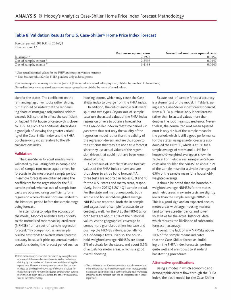
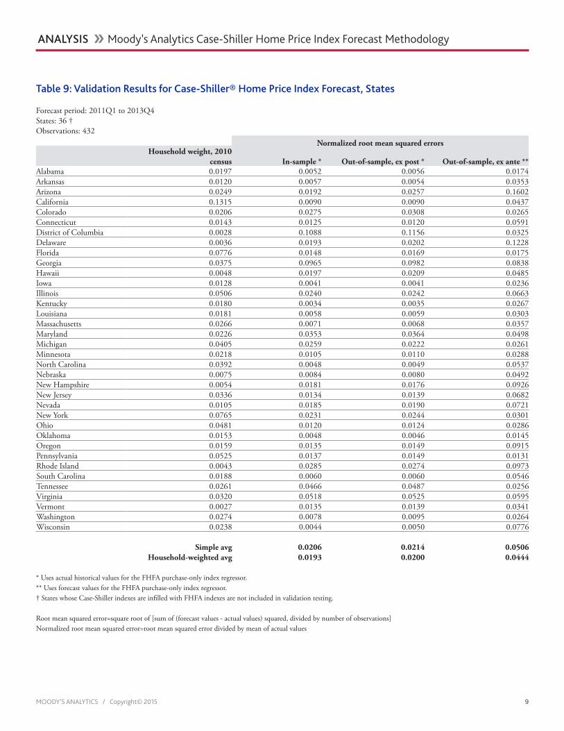
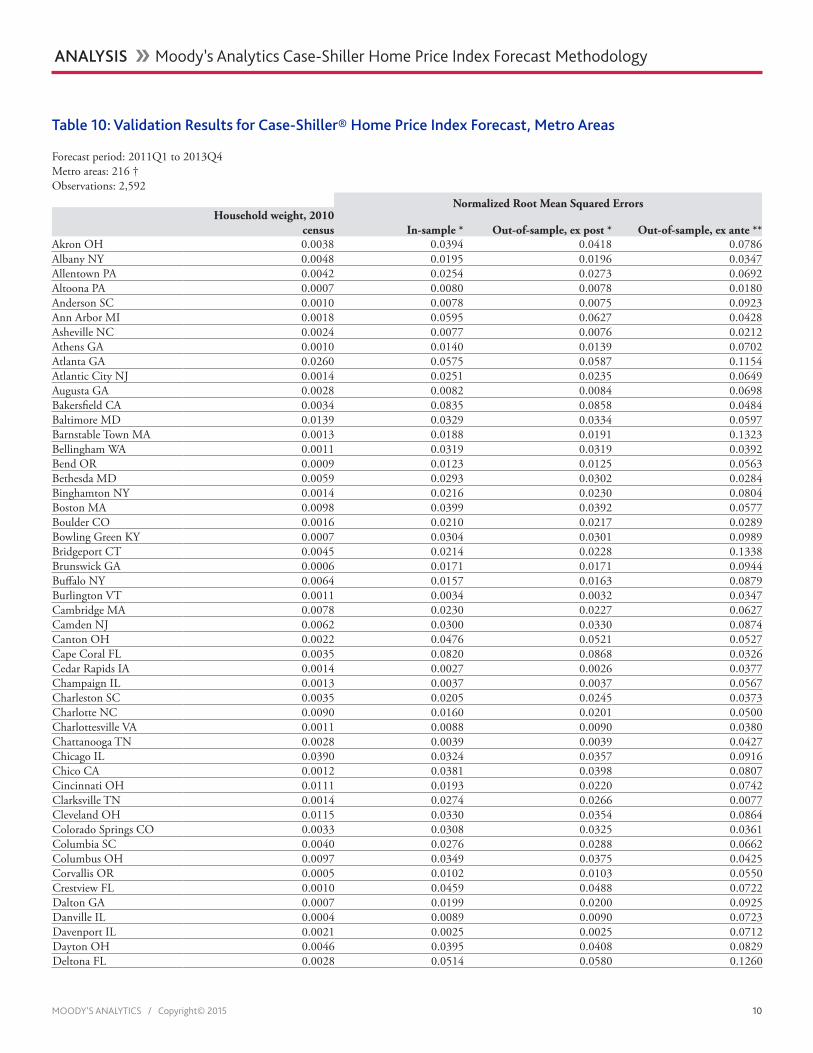
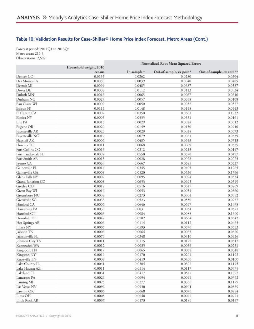
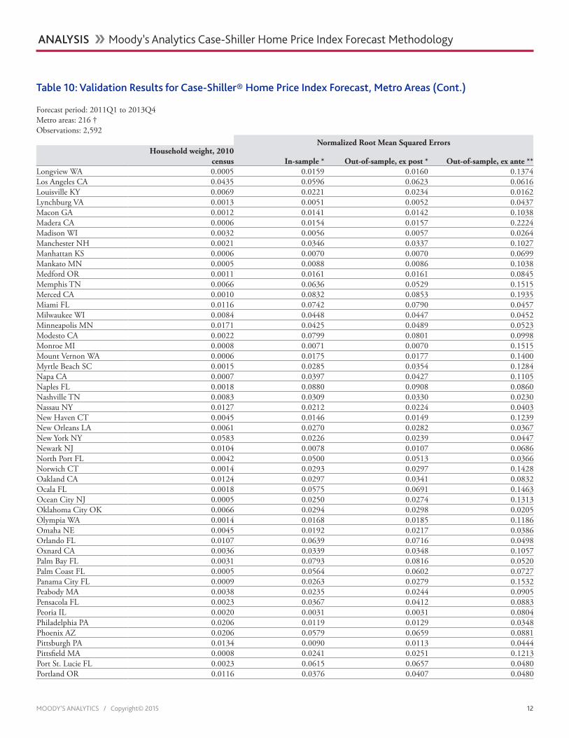
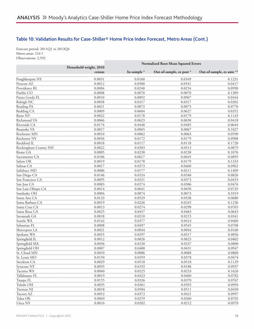
Ex ante out-of-sample tests use forecast values of the FHFA index drivers and are thus closer to a true blind forecast.11 All three tests are reported in Tables 8, 9 and 10 for the U.S., states and metro areas, respec-tively, in the 2011Q1-2014Q1 sample period. For the state and metro area pools, both simple and household-weighted average NRMSEs are reported. Both the in-sample and ex post out-of sample forecasts do ex-ceedingly well. For the U.S., the NRMSEs for both tests are about 1.5% of the historical values. As the geographical coverage be-comes more granular, outliers increase and push up the NRMSE values, especially for out-of-sample tests. Even so, the house-hold-weighted average NRMSEs are about 2% of actuals for the states, and about 3.5% of actuals for metro areas, which is a good overall showing.
11 This third test is not 100% ex ante since actual values of the other drivers such as the refinancing share of mortgage origi-nations are still being used. But these drivers have much less influence on the forecast than the co-integrated FHFA index regressors.
Ex ante, out-of-sample forecast accuracy is a sterner test of the model. In Table 8, us-ing a U.S. Case-Shiller index forecast derived from a FHFA purchase-only index forecast rather than its actual values more than doubles the root mean squared error. Never-theless, the normalized root mean squared error is only 4.4% of the sample mean for the period, which is still a good performance. For the states, using ex ante forecasts also doubled the NRMSE, which is at 5% for a simple average of states and 4.4% for a household-weighted average as shown in Table 9. For metro areas, using ex ante fore-casts also doubled the NRMSE to about 7.5% of the sample mean for a simple average and 6.6% of the sample mean for a household-weighted average.
It should be noted that the household-weighted average NRMSEs for the states and metro areas in ex-ante tests are slightly lower than the simple average NRMSEs. This is a good sign and an expected one, as metro areas with larger housing markets tend to have steadier trends and lower volatilities for the actual historical data, which reduces the likelihood of substantial forecast inaccuracy.
Overall, the lack of any NRMSEs above 10% of the sample means indicates that the Case-Shiller forecasts, build-ing on the FHFA index forecasts, perform quite well and are robust to standard backtesting procedures.
Alternative specificationsBeing a model in which economic and
demographic drivers flow through the FHFA index, the basic model for the Case-Shiller
Table 8: Validation Results for U.S. Case-Shiller® Home Price Index Forecast
Forecast period: 2011Q1 to 2014Q1Observations: 13
Root mean squared error Normalized root mean squared errorIn-sample * 2.1922 0.0152Out-of-sample, ex post * 2.2596 0.0157Out-of-sample, ex ante ** 6.4198 0.0446
* Uses actual historical values for the FHFA purchase-only index regressor.** Uses forecast values for the FHFA purchase-only index regressor.
Root mean squared error=square root of [sum of (forecast values - actual values) squared, divided by number of observations]Normalized root mean squared error=root mean squared error divided by mean of actual values
MOODY’S ANALYTICS / Copyright© 2015 9
ANALYSIS �� Moody’s Analytics Case-Shiller Home Price Index Forecast Methodology
Table 9: Validation Results for Case-Shiller® Home Price Index Forecast, States
Forecast period: 2011Q1 to 2013Q4States: 36 †Observations: 432
Normalized root mean squared errorsHousehold weight, 2010
census In-sample * Out-of-sample, ex post * Out-of-sample, ex ante **Alabama 0.0197 0.0052 0.0056 0.0174Arkansas 0.0120 0.0057 0.0054 0.0353Arizona 0.0249 0.0192 0.0257 0.1602California 0.1315 0.0090 0.0090 0.0437Colorado 0.0206 0.0275 0.0308 0.0265Connecticut 0.0143 0.0125 0.0120 0.0591District of Columbia 0.0028 0.1088 0.1156 0.0325Delaware 0.0036 0.0193 0.0202 0.1228Florida 0.0776 0.0148 0.0169 0.0175Georgia 0.0375 0.0965 0.0982 0.0838Hawaii 0.0048 0.0197 0.0209 0.0485Iowa 0.0128 0.0041 0.0041 0.0236Illinois 0.0506 0.0240 0.0242 0.0663Kentucky 0.0180 0.0034 0.0035 0.0267Louisiana 0.0181 0.0058 0.0059 0.0303Massachusetts 0.0266 0.0071 0.0068 0.0357Maryland 0.0226 0.0353 0.0364 0.0498Michigan 0.0405 0.0259 0.0222 0.0261Minnesota 0.0218 0.0105 0.0110 0.0288North Carolina 0.0392 0.0048 0.0049 0.0537Nebraska 0.0075 0.0084 0.0080 0.0492New Hampshire 0.0054 0.0181 0.0176 0.0926New Jersey 0.0336 0.0134 0.0139 0.0682Nevada 0.0105 0.0185 0.0190 0.0721New York 0.0765 0.0231 0.0244 0.0301Ohio 0.0481 0.0120 0.0124 0.0286Oklahoma 0.0153 0.0048 0.0046 0.0145Oregon 0.0159 0.0135 0.0149 0.0915Pennsylvania 0.0525 0.0137 0.0149 0.0131Rhode Island 0.0043 0.0285 0.0274 0.0973South Carolina 0.0188 0.0060 0.0060 0.0546Tennessee 0.0261 0.0466 0.0487 0.0256Virginia 0.0320 0.0518 0.0525 0.0595Vermont 0.0027 0.0135 0.0139 0.0341Washington 0.0274 0.0078 0.0095 0.0264Wisconsin 0.0238 0.0044 0.0050 0.0776
Simple avg 0.0206 0.0214 0.0506Household-weighted avg 0.0193 0.0200 0.0444
* Uses actual historical values for the FHFA purchase-only index regressor.** Uses forecast values for the FHFA purchase-only index regressor.† States whose Case-Shiller indexes are infilled with FHFA indexes are not included in validation testing.
Root mean squared error=square root of [sum of (forecast values - actual values) squared, divided by number of observations]Normalized root mean squared error=root mean squared error divided by mean of actual values
MOODY’S ANALYTICS / Copyright© 2015 10
ANALYSIS �� Moody’s Analytics Case-Shiller Home Price Index Forecast Methodology
Table 10: Validation Results for Case-Shiller® Home Price Index Forecast, Metro Areas
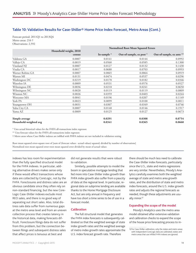
Forecast period: 2011Q1 to 2013Q4Metro areas: 216 †Observations: 2,592
Normalized Root Mean Squared ErrorsHousehold weight, 2010
census In-sample * Out-of-sample, ex post * Out-of-sample, ex ante **Akron OH 0.0038 0.0394 0.0418 0.0786Albany NY 0.0048 0.0195 0.0196 0.0347Allentown PA 0.0042 0.0254 0.0273 0.0692Altoona PA 0.0007 0.0080 0.0078 0.0180Anderson SC 0.0010 0.0078 0.0075 0.0923Ann Arbor MI 0.0018 0.0595 0.0627 0.0428Asheville NC 0.0024 0.0077 0.0076 0.0212Athens GA 0.0010 0.0140 0.0139 0.0702Atlanta GA 0.0260 0.0575 0.0587 0.1154Atlantic City NJ 0.0014 0.0251 0.0235 0.0649Augusta GA 0.0028 0.0082 0.0084 0.0698Bakersfield CA 0.0034 0.0835 0.0858 0.0484Baltimore MD 0.0139 0.0329 0.0334 0.0597Barnstable Town MA 0.0013 0.0188 0.0191 0.1323Bellingham WA 0.0011 0.0319 0.0319 0.0392Bend OR 0.0009 0.0123 0.0125 0.0563Bethesda MD 0.0059 0.0293 0.0302 0.0284Binghamton NY 0.0014 0.0216 0.0230 0.0804Boston MA 0.0098 0.0399 0.0392 0.0577Boulder CO 0.0016 0.0210 0.0217 0.0289Bowling Green KY 0.0007 0.0304 0.0301 0.0989Bridgeport CT 0.0045 0.0214 0.0228 0.1338Brunswick GA 0.0006 0.0171 0.0171 0.0944Buffalo NY 0.0064 0.0157 0.0163 0.0879Burlington VT 0.0011 0.0034 0.0032 0.0347Cambridge MA 0.0078 0.0230 0.0227 0.0627Camden NJ 0.0062 0.0300 0.0330 0.0874Canton OH 0.0022 0.0476 0.0521 0.0527Cape Coral FL 0.0035 0.0820 0.0868 0.0326Cedar Rapids IA 0.0014 0.0027 0.0026 0.0377Champaign IL 0.0013 0.0037 0.0037 0.0567Charleston SC 0.0035 0.0205 0.0245 0.0373Charlotte NC 0.0090 0.0160 0.0201 0.0500Charlottesville VA 0.0011 0.0088 0.0090 0.0380Chattanooga TN 0.0028 0.0039 0.0039 0.0427Chicago IL 0.0390 0.0324 0.0357 0.0916Chico CA 0.0012 0.0381 0.0398 0.0807Cincinnati OH 0.0111 0.0193 0.0220 0.0742Clarksville TN 0.0014 0.0274 0.0266 0.0077Cleveland OH 0.0115 0.0330 0.0354 0.0864Colorado Springs CO 0.0033 0.0308 0.0325 0.0361Columbia SC 0.0040 0.0276 0.0288 0.0662Columbus OH 0.0097 0.0349 0.0375 0.0425Corvallis OR 0.0005 0.0102 0.0103 0.0550Crestview FL 0.0010 0.0459 0.0488 0.0722Dalton GA 0.0007 0.0199 0.0200 0.0925Danville IL 0.0004 0.0089 0.0090 0.0723Davenport IL 0.0021 0.0025 0.0025 0.0712Dayton OH 0.0046 0.0395 0.0408 0.0829Deltona FL 0.0028 0.0514 0.0580 0.1260
MOODY’S ANALYTICS / Copyright© 2015 11
ANALYSIS �� Moody’s Analytics Case-Shiller Home Price Index Forecast Methodology
Table 10: Validation Results for Case-Shiller® Home Price Index Forecast, Metro Areas (Cont.)
Forecast period: 2011Q1 to 2013Q4Metro areas: 216 †Observations: 2,592
Normalized Root Mean Squared ErrorsHousehold weight, 2010
census In-sample * Out-of-sample, ex post * Out-of-sample, ex ante **Denver CO 0.0135 0.0262 0.0280 0.0304Des Moines IA 0.0030 0.0039 0.0040 0.0405Detroit MI 0.0094 0.0485 0.0687 0.0587Dover DE 0.0008 0.0112 0.0113 0.0934Duluth MN 0.0016 0.0065 0.0067 0.0616Durham NC 0.0027 0.0057 0.0058 0.0108Eau Claire WI 0.0009 0.0050 0.0052 0.0527Edison NJ 0.0115 0.0148 0.0158 0.0543El Centro CA 0.0007 0.0350 0.0361 0.1932Elmira NY 0.0005 0.0535 0.0531 0.0161Erie PA 0.0015 0.0029 0.0028 0.0612Eugene OR 0.0020 0.0149 0.0150 0.0910Fayetteville AR 0.0023 0.0029 0.0028 0.0573Fayetteville NC 0.0019 0.0079 0.0081 0.0339Flagstaff AZ 0.0006 0.0485 0.0543 0.0713Florence SC 0.0011 0.0068 0.0069 0.0535Fort Collins CO 0.0016 0.0212 0.0213 0.0147Fort Lauderdale FL 0.0092 0.0550 0.0570 0.0497Fort Smith AR 0.0015 0.0028 0.0028 0.0273Fresno CA 0.0039 0.0667 0.0685 0.0627Gainesville FL 0.0014 0.0345 0.0405 0.1265Gainesville GA 0.0008 0.0520 0.0536 0.1766Glens Falls NY 0.0007 0.0095 0.0094 0.0534Grand Junction CO 0.0008 0.0653 0.0695 0.0349Greeley CO 0.0012 0.0516 0.0547 0.0269Green Bay WI 0.0016 0.0053 0.0054 0.0860Greensboro NC 0.0039 0.0273 0.0304 0.0352Greenville SC 0.0033 0.0523 0.0550 0.0237Hanford CA 0.0006 0.0646 0.0657 0.1378Harrisburg PA 0.0030 0.0031 0.0031 0.0571Hartford CT 0.0063 0.0084 0.0088 0.1300Honolulu HI 0.0042 0.0702 0.0664 0.0642Hot Springs AR 0.0006 0.0114 0.0112 0.0465Ithaca NY 0.0005 0.0593 0.0570 0.0553Jackson TN 0.0006 0.0064 0.0065 0.0820Jacksonville FL 0.0070 0.0348 0.0410 0.0926Johnson City TN 0.0011 0.0115 0.0122 0.0512Kennewick WA 0.0012 0.0035 0.0036 0.0231Kingsport TN 0.0017 0.0065 0.0068 0.0348Kingston NY 0.0010 0.0170 0.0204 0.1192Knoxville TN 0.0038 0.0419 0.0430 0.0100Lake County IL 0.0041 0.0304 0.0307 0.1175Lake Havasu AZ 0.0011 0.0114 0.0117 0.0375Lakeland FL 0.0031 0.0417 0.0547 0.1092Lancaster PA 0.0026 0.0094 0.0094 0.0362Lansing MI 0.0025 0.0277 0.0336 0.1179Las Vegas NV 0.0096 0.0930 0.0941 0.0839Lawton OK 0.0006 0.0068 0.0070 0.0894Lima OH 0.0005 0.0048 0.0047 0.0721Little Rock AR 0.0037 0.0173 0.0180 0.0147
MOODY’S ANALYTICS / Copyright© 2015 12
ANALYSIS �� Moody’s Analytics Case-Shiller Home Price Index Forecast Methodology
Table 10: Validation Results for Case-Shiller® Home Price Index Forecast, Metro Areas (Cont.)
Forecast period: 2011Q1 to 2013Q4Metro areas: 216 †Observations: 2,592
Normalized Root Mean Squared ErrorsHousehold weight, 2010
census In-sample * Out-of-sample, ex post * Out-of-sample, ex ante **Longview WA 0.0005 0.0159 0.0160 0.1374Los Angeles CA 0.0435 0.0596 0.0623 0.0616Louisville KY 0.0069 0.0221 0.0234 0.0162Lynchburg VA 0.0013 0.0051 0.0052 0.0437Macon GA 0.0012 0.0141 0.0142 0.1038Madera CA 0.0006 0.0154 0.0157 0.2224Madison WI 0.0032 0.0056 0.0057 0.0264Manchester NH 0.0021 0.0346 0.0337 0.1027Manhattan KS 0.0006 0.0070 0.0070 0.0699Mankato MN 0.0005 0.0088 0.0086 0.1038Medford OR 0.0011 0.0161 0.0161 0.0845Memphis TN 0.0066 0.0636 0.0529 0.1515Merced CA 0.0010 0.0832 0.0853 0.1935Miami FL 0.0116 0.0742 0.0790 0.0457Milwaukee WI 0.0084 0.0448 0.0447 0.0452Minneapolis MN 0.0171 0.0425 0.0489 0.0523Modesto CA 0.0022 0.0799 0.0801 0.0998Monroe MI 0.0008 0.0071 0.0070 0.1515Mount Vernon WA 0.0006 0.0175 0.0177 0.1400Myrtle Beach SC 0.0015 0.0285 0.0354 0.1284Napa CA 0.0007 0.0397 0.0427 0.1105Naples FL 0.0018 0.0880 0.0908 0.0860Nashville TN 0.0083 0.0309 0.0330 0.0230Nassau NY 0.0127 0.0212 0.0224 0.0403New Haven CT 0.0045 0.0146 0.0149 0.1239New Orleans LA 0.0061 0.0270 0.0282 0.0367New York NY 0.0583 0.0226 0.0239 0.0447Newark NJ 0.0104 0.0078 0.0107 0.0686North Port FL 0.0042 0.0500 0.0513 0.0366Norwich CT 0.0014 0.0293 0.0297 0.1428Oakland CA 0.0124 0.0297 0.0341 0.0832Ocala FL 0.0018 0.0575 0.0691 0.1463Ocean City NJ 0.0005 0.0250 0.0274 0.1313Oklahoma City OK 0.0066 0.0294 0.0298 0.0205Olympia WA 0.0014 0.0168 0.0185 0.1186Omaha NE 0.0045 0.0192 0.0217 0.0386Orlando FL 0.0107 0.0639 0.0716 0.0498Oxnard CA 0.0036 0.0339 0.0348 0.1057Palm Bay FL 0.0031 0.0793 0.0816 0.0520Palm Coast FL 0.0005 0.0564 0.0602 0.0727Panama City FL 0.0009 0.0263 0.0279 0.1532Peabody MA 0.0038 0.0235 0.0244 0.0905Pensacola FL 0.0023 0.0367 0.0412 0.0883Peoria IL 0.0020 0.0031 0.0031 0.0804Philadelphia PA 0.0206 0.0119 0.0129 0.0348Phoenix AZ 0.0206 0.0579 0.0659 0.0881Pittsburgh PA 0.0134 0.0090 0.0113 0.0444Pittsfield MA 0.0008 0.0241 0.0251 0.1213Port St. Lucie FL 0.0023 0.0615 0.0657 0.0480Portland OR 0.0116 0.0376 0.0407 0.0480
MOODY’S ANALYTICS / Copyright© 2015 13
ANALYSIS �� Moody’s Analytics Case-Shiller Home Price Index Forecast Methodology
Table 10: Validation Results for Case-Shiller® Home Price Index Forecast, Metro Areas (Cont.)
Forecast period: 2011Q1 to 2013Q4Metro areas: 216 †Observations: 2,592
Normalized Root Mean Squared ErrorsHousehold weight, 2010
census In-sample * Out-of-sample, ex post * Out-of-sample, ex ante **
Poughkeepsie NY 0.0031 0.0160 0.0169 0.1231Prescott AZ 0.0012 0.0500 0.0541 0.0417Providence RI 0.0084 0.0248 0.0254 0.0998Pueblo CO 0.0008 0.0070 0.0070 0.1309Punta Gorda FL 0.0010 0.0892 0.0967 0.0444Raleigh NC 0.0058 0.0317 0.0317 0.0302Reading PA 0.0021 0.0072 0.0073 0.0770Redding CA 0.0009 0.0604 0.0627 0.0352Reno NV 0.0022 0.0178 0.0179 0.1143Richmond VA 0.0066 0.0623 0.0650 0.0418Riverside CA 0.0174 0.0448 0.0485 0.0644Roanoke VA 0.0017 0.0065 0.0067 0.1027Rochester MN 0.0010 0.0062 0.0063 0.0590Rochester NY 0.0056 0.0172 0.0179 0.0908Rockford IL 0.0018 0.0117 0.0118 0.1720Rockingham County NH 0.0022 0.0303 0.0313 0.0879Rome GA 0.0005 0.0230 0.0238 0.1076Sacramento CA 0.0106 0.0617 0.0645 0.0895Salem OR 0.0019 0.0178 0.0179 0.1333Salinas CA 0.0017 0.0373 0.0460 0.0962Salisbury MD 0.0006 0.0177 0.0211 0.1409San Diego CA 0.0146 0.0324 0.0340 0.0826San Francisco CA 0.0095 0.0321 0.0373 0.0453San Jose CA 0.0083 0.0274 0.0306 0.0476San Luis Obispo CA 0.0014 0.0641 0.0650 0.0745Sandusky OH 0.0004 0.0074 0.0073 0.1019Santa Ana CA 0.0133 0.0529 0.0538 0.0680Santa Barbara CA 0.0019 0.0226 0.0245 0.1236Santa Cruz CA 0.0013 0.0274 0.0298 0.0765Santa Rosa CA 0.0025 0.0457 0.0483 0.0643Savannah GA 0.0018 0.0210 0.0215 0.0341Seattle WA 0.0142 0.0377 0.0414 0.0460Sebastian FL 0.0008 0.0497 0.0545 0.0708Shreveport LA 0.0021 0.0044 0.0044 0.0160Spokane WA 0.0025 0.0297 0.0317 0.0856Springfield IL 0.0012 0.0026 0.0025 0.0402Springfield MA 0.0036 0.0230 0.0237 0.0800Springfield OH 0.0007 0.0400 0.0431 0.0947St. Cloud MN 0.0010 0.0086 0.0088 0.0868St. Louis MO 0.0150 0.0359 0.0378 0.0474Stockton CA 0.0029 0.0510 0.0518 0.1139Syracuse NY 0.0035 0.0192 0.0186 0.0937Tacoma WA 0.0040 0.0225 0.0233 0.1626Tallahassee FL 0.0019 0.0423 0.0460 0.0782Tampa FL 0.0155 0.0326 0.0370 0.0767Toledo OH 0.0035 0.0361 0.0392 0.0994Trenton NJ 0.0018 0.0504 0.0511 0.0450Tucson AZ 0.0052 0.0372 0.0421 0.0997Tulsa OK 0.0049 0.0259 0.0260 0.0702Utica NY 0.0016 0.0202 0.0212 0.0970
MOODY’S ANALYTICS / Copyright© 2015 14
ANALYSIS �� Moody’s Analytics Case-Shiller Home Price Index Forecast Methodology
Table 10: Validation Results for Case-Shiller® Home Price Index Forecast, Metro Areas (Cont.)
Forecast period: 2011Q1 to 2013Q4Metro areas: 216 †Observations: 2,592
Normalized Root Mean Squared ErrorsHousehold weight, 2010
census In-sample * Out-of-sample, ex post * Out-of-sample, ex ante **
Valdosta GA 0.0007 0.0141 0.0144 0.0992Vallejo CA 0.0019 0.0560 0.0585 0.1300Vineland NJ 0.0007 0.0127 0.0132 0.1430Visalia CA 0.0017 0.0680 0.0703 0.0993Warner Robins GA 0.0007 0.0065 0.0064 0.0919Warren MI 0.0131 0.0474 0.0537 0.0296Washington DC 0.0219 0.0178 0.0182 0.0346Waterloo IA 0.0009 0.0531 0.0576 0.0527Wilmington DE 0.0036 0.0218 0.0241 0.0650Wilmington NC 0.0020 0.0119 0.0119 0.0809Winston NC 0.0026 0.0359 0.0403 0.0244Worcester MA 0.0041 0.0196 0.0207 0.1149York PA 0.0023 0.0099 0.0100 0.0811Youngstown OH 0.0031 0.0307 0.0349 0.0746Yuba City CA 0.0007 0.0148 0.0146 0.1917Yuma AZ 0.0009 0.0125 0.0127 0.0673
Simple average 0.0291 0.0308 0.0754Household-weighted avg 0.0341 0.0365 0.0660
* Uses actual historical values for the FHFA all-transactions index regressor.** Uses forecast values for the FHFA all-transactions index regressor.† Metro areas whose Case-Shiller indexes are infilled with FHFA indexes are not included in validation testing
Root mean squared error=square root of [sum of (forecast values - actual values) squared, divided by number of observations]Normalized root mean squared error=root mean squared error divided by mean of actual values
indexes has less room for experimentation than the fully specified structural model for the FHFA indexes. In particular, add-ing alternative drivers makes sense only if these would affect transactions whose data are collected by CoreLogic, not by the FHFA. Foreclosures and distress sales are an obvious candidate since they often rely on non-standard financing, but the new Core-Logic Case-Shiller indexes exclude most REO sales, and there is no good way of separating out short sales. Also, total dis-tress sale data suffer from numerous gaps at the metro area level and from an uneven collection process that creates latency in the historical data, making forecasts dif-ficult. Foreclosure filings data do not suffer from this problem, but the connection be-tween filings and subsequent distress sales that affect prices is tenuous at best and
did not generate results that were robust to validation.
Similarly, possible attempts to model the boom in speculative mortgage lending that fed more into Case-Shiller index growth than FHFA index growth also suffer from a paucity of data at the regional level. In particular, re-gional data on subprime lending are available thanks to the Home Mortgage Disclosure Act, but are only annual in frequency and have too short a time series to be of use in a forecast model.
CalibrationThe full structural model that generates
the FHFA index forecasts is subsequently cal-ibrated so that the weighted average of state index growth rates and the weighted average of metro index growth rates approximate the U.S. index forecast growth rate. Therefore
there should be much less need to calibrate the Case-Shiller index forecasts, particularly since the U.S., state and metro regressions are very similar. Nevertheless, Moody’s Ana-lytics carefully examines both the weighted average of state and metro area growth rates, and the distribution of state and metro index forecasts, around the U.S. index growth rates and adjusts the regional forecasts as needed, though these adjustments are usu-ally minor.12
expanding the scope of the modelMoody’s Analytics uses the metro area
model obtained after extensive validation and calibration checks to expand the scope of the house price forecasting process to in-
12 For Case-Shiller calibration, only the states and metro areas with independent CoreLogic data are calibrated; states and metro areas that use infilled FHFA indexes are ignored.
MOODY’S ANALYTICS / Copyright© 2015 15
ANALYSIS �� Moody’s Analytics Case-Shiller Home Price Index Forecast Methodology
clude different levels of geography (regions, counties and ZIP codes) and other price measures (condo indexes and single-family indexes by price tier). This section describes the forecast process for these additional price measures.
Census divisions, msAs with divisionsFor larger geographies, the Case-Shiller
forecast is obtained through an aggregation process. For census division Case-Shiller indexes, the forecast is obtained by taking a household-weighted average of the CSI growth rates for each state in the census division, and then applying that average growth rate to the census division’s CSI his-tory.13
Similarly for metropolitan statistical ar-eas with metro divisions, the CSI forecast is obtained by growing out the index history with a household-weighted average growth rate of the CSI forecasts for each metro divi-sion within the MSA.
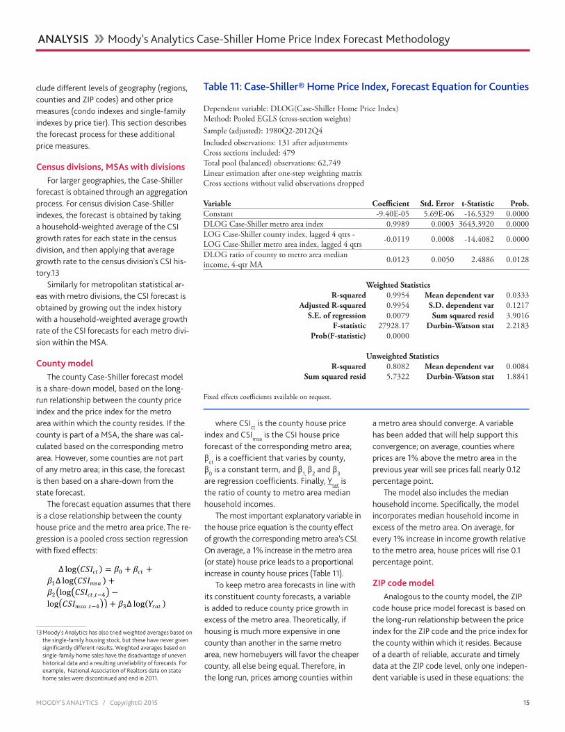
County modelThe county Case-Shiller forecast model
is a share-down model, based on the long-run relationship between the county price index and the price index for the metro area within which the county resides. If the county is part of a MSA, the share was cal-culated based on the corresponding metro area. However, some counties are not part of any metro area; in this case, the forecast is then based on a share-down from the state forecast.
The forecast equation assumes that there is a close relationship between the county house price and the metro area price. The re-gression is a pooled cross section regression with fixed effects:
Δ log(𝐶𝐶𝐶𝐶𝐶𝐶𝑐𝑐𝑡𝑡) = 𝛽𝛽0 + 𝛽𝛽𝑐𝑐𝑡𝑡 +𝛽𝛽1Δ log(𝐶𝐶𝐶𝐶𝐶𝐶𝑚𝑚𝑚𝑚𝑚𝑚 ) +𝛽𝛽2�log�𝐶𝐶𝐶𝐶𝐶𝐶𝑐𝑐𝑡𝑡 ,𝑡𝑡−4� −log�𝐶𝐶𝐶𝐶𝐶𝐶𝑚𝑚𝑚𝑚𝑚𝑚 ,𝑡𝑡−4�� + 𝛽𝛽3Δ log(𝑌𝑌𝑟𝑟𝑚𝑚𝑡𝑡 )
13 Moody’s Analytics has also tried weighted averages based on the single-family housing stock, but these have never given significantly different results. Weighted averages based on single-family home sales have the disadvantage of uneven historical data and a resulting unreliability of forecasts. For example, National Association of Realtors data on state home sales were discontinued and end in 2011.
where CSIct is the county house price index and CSImsa is the CSI house price forecast of the corresponding metro area; βct is a coefficient that varies by county, β0 is a constant term, and β1, β2 and β3 are regression coefficients. Finally, Yrat is the ratio of county to metro area median household incomes.
The most important explanatory variable in the house price equation is the county effect of growth the corresponding metro area’s CSI. On average, a 1% increase in the metro area (or state) house price leads to a proportional increase in county house prices (Table 11).
To keep metro area forecasts in line with its constituent county forecasts, a variable is added to reduce county price growth in excess of the metro area. Theoretically, if housing is much more expensive in one county than another in the same metro area, new homebuyers will favor the cheaper county, all else being equal. Therefore, in the long run, prices among counties within
a metro area should converge. A variable has been added that will help support this convergence; on average, counties where prices are 1% above the metro area in the previous year will see prices fall nearly 0.12 percentage point.
The model also includes the median household income. Specifically, the model incorporates median household income in excess of the metro area. On average, for every 1% increase in income growth relative to the metro area, house prices will rise 0.1 percentage point.
ZiP code modelAnalogous to the county model, the ZIP
code house price model forecast is based on the long-run relationship between the price index for the ZIP code and the price index for the county within which it resides. Because of a dearth of reliable, accurate and timely data at the ZIP code level, only one indepen-dent variable is used in these equations: the
Table 11: Case-Shiller® Home Price Index, Forecast Equation for Counties
Dependent variable: DLOG(Case-Shiller Home Price Index)Method: Pooled EGLS (cross-section weights)Sample (adjusted): 1980Q2-2012Q4Included observations: 131 after adjustmentsCross sections included: 479Total pool (balanced) observations: 62,749Linear estimation after one-step weighting matrixCross sections without valid observations dropped
Variable Coefficient Std. Error t-Statistic Prob. Constant -9.40E-05 5.69E-06 -16.5329 0.0000DLOG Case-Shiller metro area index 0.9989 0.0003 3643.3920 0.0000LOG Case-Shiller county index, lagged 4 qtrs - LOG Case-Shiller metro area index, lagged 4 qtrs -0.0119 0.0008 -14.4082 0.0000
DLOG ratio of county to metro area median income, 4-qtr MA 0.0123 0.0050 2.4886 0.0128
Weighted StatisticsR-squared 0.9954 Mean dependent var 0.0333
Adjusted R-squared 0.9954 S.D. dependent var 0.1217S.E. of regression 0.0079 Sum squared resid 3.9016
F-statistic 27928.17 Durbin-Watson stat 2.2183Prob(F-statistic) 0.0000
Unweighted StatisticsR-squared 0.8082 Mean dependent var 0.0084
Sum squared resid 5.7322 Durbin-Watson stat 1.8841
Fixed effects coefficients available on request.
MOODY’S ANALYTICS / Copyright© 2015 16
ANALYSIS �� Moody’s Analytics Case-Shiller Home Price Index Forecast Methodology
house price index in the county in which the ZIP code lies. In the situation where histori-cal ZIP code data exist but the county’s do not, the metro area forecast is used. If the ZIP code is not within a metro area, the state forecast is used.
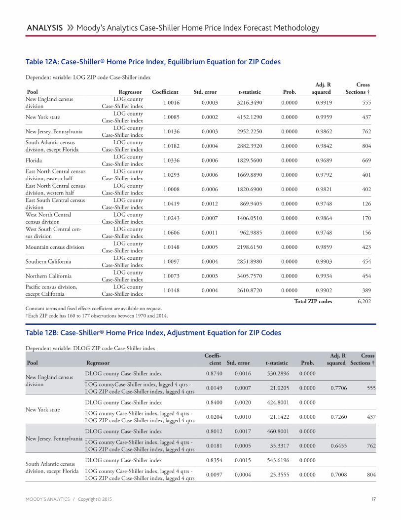
The ZIP code forecast model is a two-stage model. In the first step, an equilibrium equation is established. The equilibrium equation assumes there is a close relation-ship between the ZIP code house price and county price levels over the long term. The regression is a pool cross-sectional regres-sion with fixed effects:
log�𝐶𝐶𝐶𝐶𝐶𝐶𝑧𝑧𝑧𝑧𝑧𝑧 � = 𝛽𝛽0 + 𝛽𝛽𝑧𝑧𝑧𝑧𝑧𝑧 + 𝛽𝛽1log(𝐶𝐶𝐶𝐶𝐶𝐶𝑐𝑐𝑡𝑡)
where CSIzip is the ZIP code house price index and CSIct is the Case-Shiller house price forecast of the corresponding county; β0 is a constant term that varies by broad geo-graphical region as described below, βzip is a coefficient that varies by ZIP code, and β1 is a regression coefficient.
In the second stage, an adjustment equa-tion is established. The basis for the adjust-ment equation is that growth rate in the ZIP code will mimic that in the corresponding county. Like the equilibrium equation, the re-gression is a pool cross-sectional regression with fixed effects:
Δlog�𝐶𝐶𝐶𝐶𝐶𝐶𝑧𝑧𝑧𝑧𝑧𝑧 � = 𝛽𝛽0 + 𝛽𝛽𝑧𝑧𝑧𝑧𝑧𝑧 +𝛽𝛽1Δ log(𝐶𝐶𝐶𝐶𝐶𝐶𝑐𝑐𝑡𝑡) +𝛽𝛽2(log�𝐶𝐶𝐶𝐶𝐶𝐶𝑐𝑐𝑡𝑡 ,𝑡𝑡−4� − log�𝐶𝐶𝐶𝐶𝐶𝐶𝑧𝑧𝑧𝑧𝑧𝑧 ,𝑡𝑡−4�)
with similar notation, and the addition of β2 as the coefficient of the adjustment term, which is also lagged four quarters. In the final step, the forecast from the adjust-ment equation reverts to the forecast from the equilibrium equation through a mean reversion process.
Fourteen pools have been constructed across the 6,200 ZIP code areas included in the estimation. The pools are based on ge-ography, with separate pools for each census division. The East North Central division is fur-ther broken down into eastern (Ohio, Indiana, and parts of Michigan) and western (Illinois, Wisconsin, and most of Michigan) pools. Fur-ther, there are separate pools for Florida, New
York and California, which is also broken down into northern and southern halves.
The classification of the regions is based on the idea that these areas share long-run trends of demographics and economic com-position. The pooling creates a large number of observations to allow for greater localiza-tion of the variables included in the estima-tion, although the pools vary by size. The large number of observations also improves the accuracy of the model estimation.
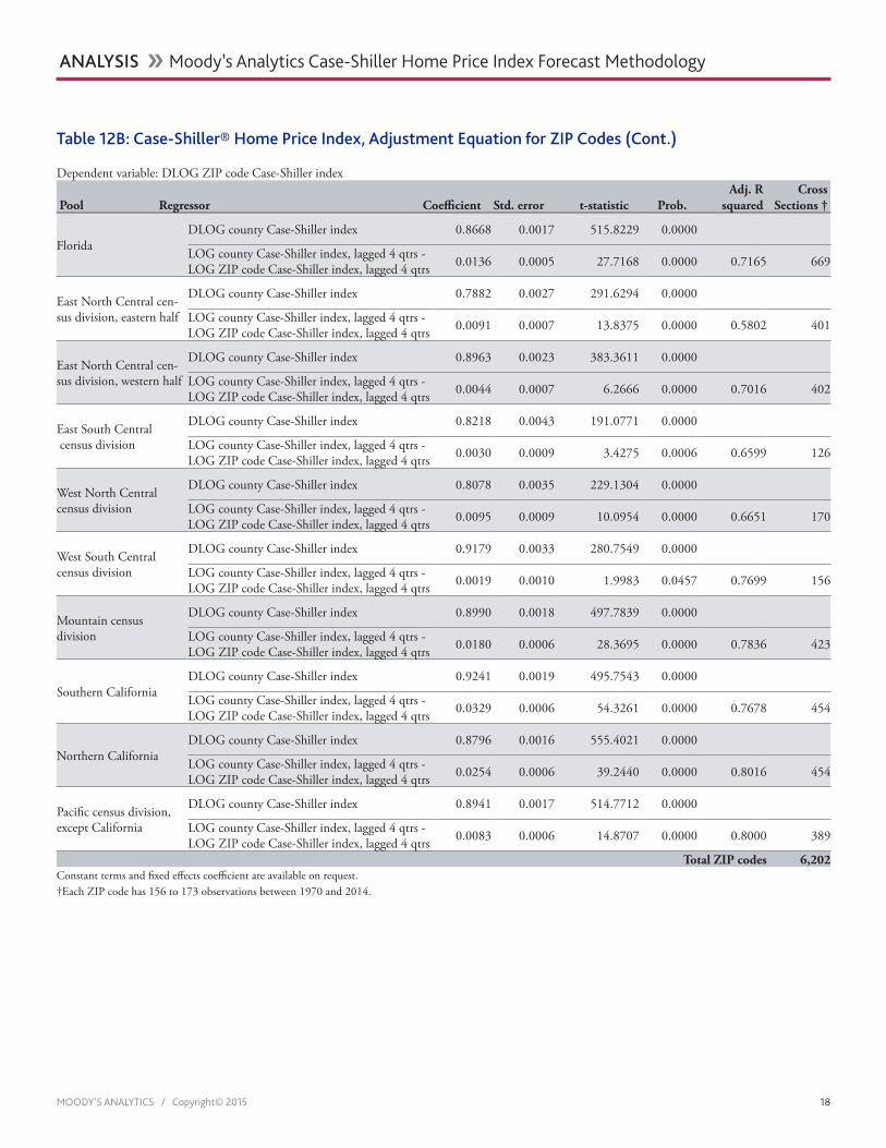
Tables 12A and 12B show the regression results for all 14 pools. The results in Table 12A are singularly uniform: The higher the county house price, the higher the ZIP code house price, with the coefficient varying between 1 and 1.06. Also, the large number of observations and the use of fixed effects almost guarantee that the adjusted R^2 sta-tistic for each pooled regression will be close to 1. This relative uniformity occurs despite the uneven distribution of ZIP codes in the historical data, with the Great Plains states in particular being underrepresented because of nondisclosure laws.
Table 12B shows the result of the adjust-ment equation regressions. The faster the county house price has been rising relative to the ZIP code house price, the faster the ZIP code house price will appreciate. This is con-firmed with the results, with all pools having coefficients for the county index driver of between 0.8 and 0.9. In addition, the er-ror correction term is positive and points to gradual reversion of the ZIP code to the county indexes of between 0.5% and 3% per quarter, depending on the region.
Condo and price tier models Separate models are also developed for
forecasting house prices of condominiums and tiers. The forecast equation assumes that condos and tiers prices within a metro area would move in sync with the broader hous-ing market of the metro area.14 Since these price indexes represent specific segments
14 With new data available from CoreLogic, the Case-Shiller indexes have recently expanded condo index coverage to states, and tier index coverage to states, census divisions, and counties. Regardless of geographical coverage, the same pooled regression specifications are used. For simplicity, the following discussion assumes that only metro area indexes are being considered.
of a metro area’s housing market, and the metro area aggregate single-family house price is a good indicator of the larger market, the metro area price index is a main driver of the condo and tier forecast models. As with standard error correction models, the lagged difference in the condo and aggregate single-family indexes is also a good prediction of reversion tendencies, as condo prices cannot indefinitely stay too high or too low com-pared with single-family prices. Since condo purchases tend to rely more on conventional mortgage financing, a user cost driver is also included to explain deviations in the index’s growth path relative to the aggregate index.
The condo regression is a pooled cross-section regression with fixed effects:
∆log(𝐶𝐶𝐶𝐶𝐶𝐶𝑐𝑐𝑐𝑐 ) = 𝛽𝛽0 + 𝛽𝛽1 ∆log(𝐶𝐶𝐶𝐶𝐶𝐶𝑚𝑚𝑚𝑚𝑚𝑚 ) +𝛽𝛽2�log�𝐶𝐶𝐶𝐶𝐶𝐶𝑐𝑐𝑐𝑐 ,𝑡𝑡−1� − log�𝐶𝐶𝐶𝐶𝐶𝐶𝑚𝑚𝑚𝑚𝑚𝑚 ,𝑡𝑡−1�� + 𝛽𝛽3𝑈𝑈𝐶𝐶𝑚𝑚𝑚𝑚𝑚𝑚
where CSIco is the condo house price index and CSImsa is the aggregate Case-Shiller house price for the corresponding metro area; β0 is a constant term, β1, β2 and β3 are the other regression coefficients. UCmsa is the after-tax user cost of owning a home in a metro area, calculated as a tax-adjusted ef-fective composite mortgage rate minus the rate of core inflation.
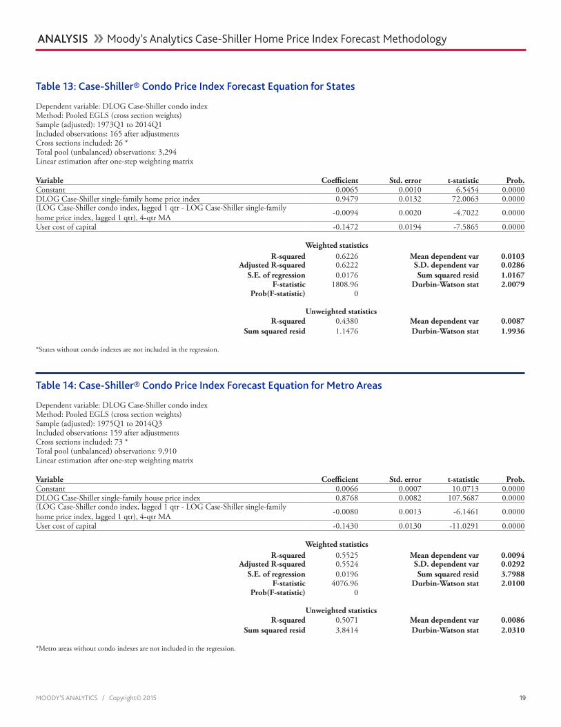
Tables 13 and 14 present the regression results for state and metro area condo in-dexes. The most important explanatory vari-able in the condo house price equation is the metro area’s Case-Shiller house price index. On average, a 1% increase in the metro fore-cast leads to an approximately 0.9 percent-age point increase in condo house prices. On the other hand, the user cost of owning a home, which takes into account institutional variables such as property taxes, mortgage rates, and maintenance and obsolescence, adds information to the regression and is negatively related to prices. Therefore, as user costs increase, individuals prefer to rent rather than own a condo unit. Finally, while the reversion term is statistically significant and of the right sign, it has only a weak ef-fect, indicating that deviations of condo pric-es from the single-family index take many years to correct.
MOODY’S ANALYTICS / Copyright© 2015 17
ANALYSIS �� Moody’s Analytics Case-Shiller Home Price Index Forecast Methodology
Table 12B: Case-Shiller® Home Price Index, Adjustment Equation for ZIP Codes
Dependent variable: DLOG ZIP code Case-Shiller index
Pool RegressorCoeffi-
cient Std. error t-statistic Prob.Adj. R
squaredCross
Sections †
New England census division
DLOG county Case-Shiller index 0.8740 0.0016 530.2896 0.0000
LOG countyCase-Shiller index, lagged 4 qtrs - LOG ZIP code Case-Shiller index, lagged 4 qtrs 0.0149 0.0007 21.0205 0.0000 0.7706 555
New York stateDLOG county Case-Shiller index 0.8400 0.0020 424.8001 0.0000
LOG county Case-Shiller index, lagged 4 qtrs - LOG ZIP code Case-Shiller index, lagged 4 qtrs 0.0204 0.0010 21.1422 0.0000 0.7260 437
New Jersey, PennsylvaniaDLOG county Case-Shiller index 0.8012 0.0017 460.8001 0.0000
LOG county Case-Shiller index, lagged 4 qtrs - LOG ZIP code Case-Shiller index, lagged 4 qtrs 0.0181 0.0005 35.3317 0.0000 0.6455 762
South Atlantic census division, except Florida
DLOG county Case-Shiller index 0.8354 0.0015 543.6196 0.0000
LOG county Case-Shiller index, lagged 4 qtrs - LOG ZIP code Case-Shiller index, lagged 4 qtrs 0.0097 0.0004 25.3555 0.0000 0.7008 804
Table 12A: Case-Shiller® Home Price Index, Equilibrium Equation for ZIP Codes
Dependent variable: LOG ZIP code Case-Shiller index
Pool Regressor Coefficient Std. error t-statistic Prob.Adj. R
squaredCross
Sections †New England census division
LOG county Case-Shiller index 1.0016 0.0003 3216.3490 0.0000 0.9919 555
New York state LOG county Case-Shiller index 1.0085 0.0002 4152.1290 0.0000 0.9959 437
New Jersey, Pennsylvania LOG county Case-Shiller index 1.0136 0.0003 2952.2250 0.0000 0.9862 762
South Atlantic census division, except Florida
LOG county Case-Shiller index 1.0182 0.0004 2882.3920 0.0000 0.9842 804
Florida LOG county Case-Shiller index 1.0336 0.0006 1829.5600 0.0000 0.9689 669
East North Central census division, eastern half
LOG county Case-Shiller index 1.0293 0.0006 1669.8890 0.0000 0.9792 401
East North Central census division, western half
LOG county Case-Shiller index 1.0008 0.0006 1820.6900 0.0000 0.9821 402
East South Central census division
LOG county Case-Shiller index 1.0419 0.0012 869.9405 0.0000 0.9748 126
West North Central census division
LOG county Case-Shiller index 1.0243 0.0007 1406.0510 0.0000 0.9864 170
West South Central cen-sus division
LOG county Case-Shiller index 1.0606 0.0011 962.9885 0.0000 0.9748 156
Mountain census division LOG county Case-Shiller index 1.0148 0.0005 2198.6150 0.0000 0.9859 423
Southern California LOG county Case-Shiller index 1.0097 0.0004 2851.8980 0.0000 0.9903 454
Northern California LOG county Case-Shiller index 1.0073 0.0003 3405.7570 0.0000 0.9934 454
Pacific census division, except California
LOG county Case-Shiller index 1.0148 0.0004 2610.8720 0.0000 0.9902 389
Total ZIP codes 6,202Constant terms and fixed effects coefficient are available on request.†Each ZIP code has 160 to 177 observations between 1970 and 2014.
MOODY’S ANALYTICS / Copyright© 2015 18
ANALYSIS �� Moody’s Analytics Case-Shiller Home Price Index Forecast Methodology
FloridaDLOG county Case-Shiller index 0.8668 0.0017 515.8229 0.0000
LOG county Case-Shiller index, lagged 4 qtrs - LOG ZIP code Case-Shiller index, lagged 4 qtrs 0.0136 0.0005 27.7168 0.0000 0.7165 669
East North Central cen-sus division, eastern half
DLOG county Case-Shiller index 0.7882 0.0027 291.6294 0.0000
LOG county Case-Shiller index, lagged 4 qtrs - LOG ZIP code Case-Shiller index, lagged 4 qtrs 0.0091 0.0007 13.8375 0.0000 0.5802 401
East North Central cen-sus division, western half
DLOG county Case-Shiller index 0.8963 0.0023 383.3611 0.0000
LOG county Case-Shiller index, lagged 4 qtrs - LOG ZIP code Case-Shiller index, lagged 4 qtrs 0.0044 0.0007 6.2666 0.0000 0.7016 402
East South Central census division
DLOG county Case-Shiller index 0.8218 0.0043 191.0771 0.0000
LOG county Case-Shiller index, lagged 4 qtrs - LOG ZIP code Case-Shiller index, lagged 4 qtrs 0.0030 0.0009 3.4275 0.0006 0.6599 126
West North Central census division
DLOG county Case-Shiller index 0.8078 0.0035 229.1304 0.0000
LOG county Case-Shiller index, lagged 4 qtrs - LOG ZIP code Case-Shiller index, lagged 4 qtrs 0.0095 0.0009 10.0954 0.0000 0.6651 170
West South Central census division
DLOG county Case-Shiller index 0.9179 0.0033 280.7549 0.0000
LOG county Case-Shiller index, lagged 4 qtrs - LOG ZIP code Case-Shiller index, lagged 4 qtrs 0.0019 0.0010 1.9983 0.0457 0.7699 156
Mountain census division
DLOG county Case-Shiller index 0.8990 0.0018 497.7839 0.0000
LOG county Case-Shiller index, lagged 4 qtrs - LOG ZIP code Case-Shiller index, lagged 4 qtrs 0.0180 0.0006 28.3695 0.0000 0.7836 423
Southern CaliforniaDLOG county Case-Shiller index 0.9241 0.0019 495.7543 0.0000
LOG county Case-Shiller index, lagged 4 qtrs - LOG ZIP code Case-Shiller index, lagged 4 qtrs 0.0329 0.0006 54.3261 0.0000 0.7678 454
Northern CaliforniaDLOG county Case-Shiller index 0.8796 0.0016 555.4021 0.0000
LOG county Case-Shiller index, lagged 4 qtrs - LOG ZIP code Case-Shiller index, lagged 4 qtrs 0.0254 0.0006 39.2440 0.0000 0.8016 454
Pacific census division, except California
DLOG county Case-Shiller index 0.8941 0.0017 514.7712 0.0000
LOG county Case-Shiller index, lagged 4 qtrs - LOG ZIP code Case-Shiller index, lagged 4 qtrs 0.0083 0.0006 14.8707 0.0000 0.8000 389
Total ZIP codes 6,202Constant terms and fixed effects coefficient are available on request.†Each ZIP code has 156 to 173 observations between 1970 and 2014.
Table 12B: Case-Shiller® Home Price Index, Adjustment Equation for ZIP Codes (Cont.)
Dependent variable: DLOG ZIP code Case-Shiller index
Pool Regressor Coefficient Std. error t-statistic Prob.Adj. R
squaredCross
Sections †
MOODY’S ANALYTICS / Copyright© 2015 19
ANALYSIS �� Moody’s Analytics Case-Shiller Home Price Index Forecast Methodology
Table 13: Case-Shiller® Condo Price Index Forecast Equation for States
Dependent variable: DLOG Case-Shiller condo indexMethod: Pooled EGLS (cross section weights)Sample (adjusted): 1973Q1 to 2014Q1Included observations: 165 after adjustmentsCross sections included: 26 *Total pool (unbalanced) observations: 3,294Linear estimation after one-step weighting matrix
Variable Coefficient Std. error t-statistic Prob. Constant 0.0065 0.0010 6.5454 0.0000DLOG Case-Shiller single-family home price index 0.9479 0.0132 72.0063 0.0000(LOG Case-Shiller condo index, lagged 1 qtr - LOG Case-Shiller single-family home price index, lagged 1 qtr), 4-qtr MA -0.0094 0.0020 -4.7022 0.0000
User cost of capital -0.1472 0.0194 -7.5865 0.0000
Weighted statisticsR-squared 0.6226 Mean dependent var 0.0103
Adjusted R-squared 0.6222 S.D. dependent var 0.0286S.E. of regression 0.0176 Sum squared resid 1.0167
F-statistic 1808.96 Durbin-Watson stat 2.0079Prob(F-statistic) 0
Unweighted statisticsR-squared 0.4380 Mean dependent var 0.0087
Sum squared resid 1.1476 Durbin-Watson stat 1.9936
*States without condo indexes are not included in the regression.
Table 14: Case-Shiller® Condo Price Index Forecast Equation for Metro Areas
Dependent variable: DLOG Case-Shiller condo indexMethod: Pooled EGLS (cross section weights)Sample (adjusted): 1975Q1 to 2014Q3Included observations: 159 after adjustmentsCross sections included: 73 *Total pool (unbalanced) observations: 9,910Linear estimation after one-step weighting matrix
Variable Coefficient Std. error t-statistic Prob. Constant 0.0066 0.0007 10.0713 0.0000DLOG Case-Shiller single-family house price index 0.8768 0.0082 107.5687 0.0000(LOG Case-Shiller condo index, lagged 1 qtr - LOG Case-Shiller single-family home price index, lagged 1 qtr), 4-qtr MA -0.0080 0.0013 -6.1461 0.0000
User cost of capital -0.1430 0.0130 -11.0291 0.0000
Weighted statisticsR-squared 0.5525 Mean dependent var 0.0094
Adjusted R-squared 0.5524 S.D. dependent var 0.0292S.E. of regression 0.0196 Sum squared resid 3.7988
F-statistic 4076.96 Durbin-Watson stat 2.0100Prob(F-statistic) 0
Unweighted statisticsR-squared 0.5071 Mean dependent var 0.0086
Sum squared resid 3.8414 Durbin-Watson stat 2.0310
*Metro areas without condo indexes are not included in the regression.
MOODY’S ANALYTICS / Copyright© 2015 20
ANALYSIS �� Moody’s Analytics Case-Shiller Home Price Index Forecast Methodology
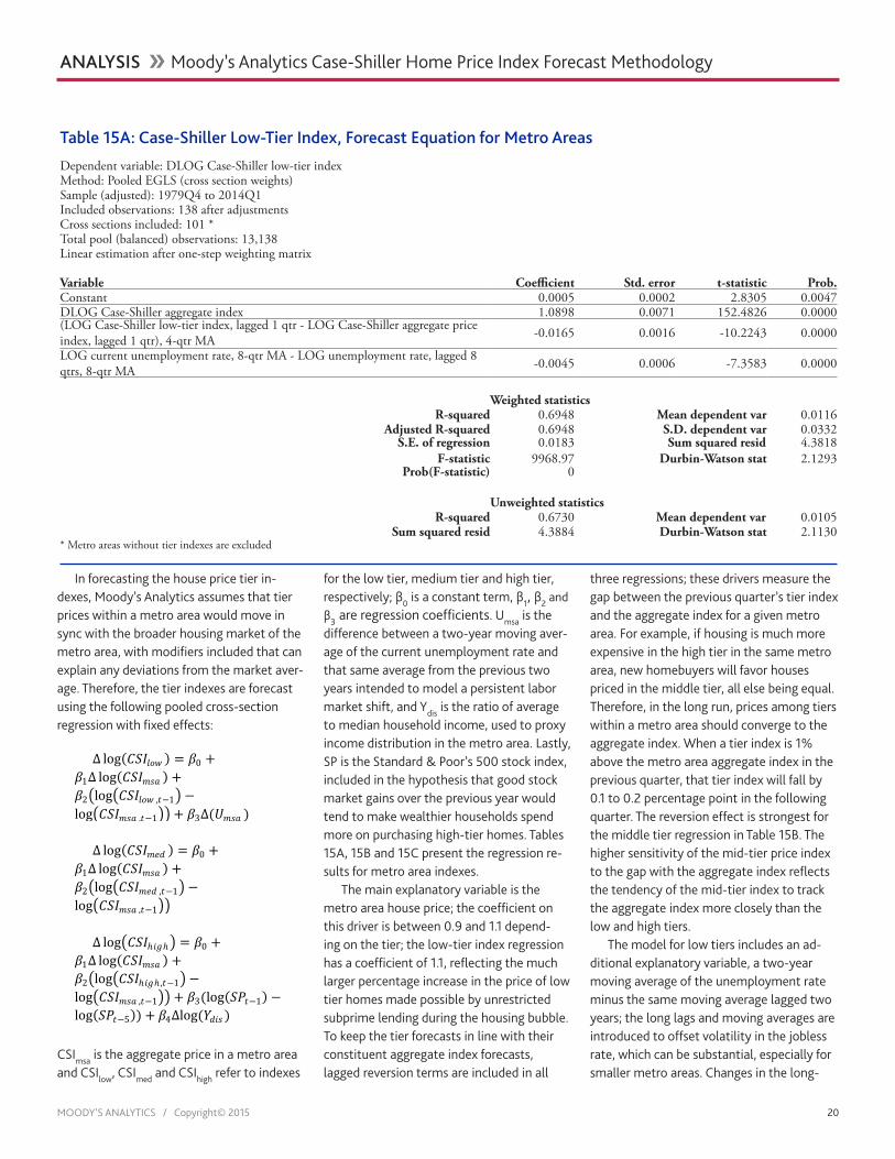
In forecasting the house price tier in-dexes, Moody’s Analytics assumes that tier prices within a metro area would move in sync with the broader housing market of the metro area, with modifiers included that can explain any deviations from the market aver-age. Therefore, the tier indexes are forecast using the following pooled cross-section regression with fixed effects:
Δ log(𝐶𝐶𝐶𝐶𝐶𝐶𝑙𝑙𝑐𝑐𝑙𝑙 ) = 𝛽𝛽0 +𝛽𝛽1Δ log(𝐶𝐶𝐶𝐶𝐶𝐶𝑚𝑚𝑚𝑚𝑚𝑚 ) +𝛽𝛽2�log�𝐶𝐶𝐶𝐶𝐶𝐶𝑙𝑙𝑐𝑐𝑙𝑙 ,𝑡𝑡−1� −log�𝐶𝐶𝐶𝐶𝐶𝐶𝑚𝑚𝑚𝑚𝑚𝑚 ,𝑡𝑡−1�� + 𝛽𝛽3Δ(𝑈𝑈𝑚𝑚𝑚𝑚𝑚𝑚 )
Δ log(𝐶𝐶𝐶𝐶𝐶𝐶𝑚𝑚𝑚𝑚𝑚𝑚 ) = 𝛽𝛽0 +𝛽𝛽1Δ log(𝐶𝐶𝐶𝐶𝐶𝐶𝑚𝑚𝑚𝑚𝑚𝑚 ) +𝛽𝛽2�log�𝐶𝐶𝐶𝐶𝐶𝐶𝑚𝑚𝑚𝑚𝑚𝑚 ,𝑡𝑡−1� −log�𝐶𝐶𝐶𝐶𝐶𝐶𝑚𝑚𝑚𝑚𝑚𝑚 ,𝑡𝑡−1��
Δ log�𝐶𝐶𝐶𝐶𝐶𝐶ℎ𝑧𝑧𝑖𝑖ℎ� = 𝛽𝛽0 +𝛽𝛽1Δ log(𝐶𝐶𝐶𝐶𝐶𝐶𝑚𝑚𝑚𝑚𝑚𝑚 ) +𝛽𝛽2�log�𝐶𝐶𝐶𝐶𝐶𝐶ℎ𝑧𝑧𝑖𝑖ℎ ,𝑡𝑡−1� −log�𝐶𝐶𝐶𝐶𝐶𝐶𝑚𝑚𝑚𝑚𝑚𝑚 ,𝑡𝑡−1�� + 𝛽𝛽3(log(𝐶𝐶𝑆𝑆𝑡𝑡−1) −log(𝐶𝐶𝑆𝑆𝑡𝑡−5)) + 𝛽𝛽4Δlog(𝑌𝑌𝑚𝑚𝑧𝑧𝑚𝑚 )
CSImsa is the aggregate price in a metro area and CSIlow, CSImed and CSIhigh refer to indexes
for the low tier, medium tier and high tier, respectively; β0 is a constant term, β1, β2 and β3 are regression coefficients. Umsa is the difference between a two-year moving aver-age of the current unemployment rate and that same average from the previous two years intended to model a persistent labor market shift, and Ydis is the ratio of average to median household income, used to proxy income distribution in the metro area. Lastly, SP is the Standard & Poor’s 500 stock index, included in the hypothesis that good stock market gains over the previous year would tend to make wealthier households spend more on purchasing high-tier homes. Tables 15A, 15B and 15C present the regression re-sults for metro area indexes.
The main explanatory variable is the metro area house price; the coefficient on this driver is between 0.9 and 1.1 depend-ing on the tier; the low-tier index regression has a coefficient of 1.1, reflecting the much larger percentage increase in the price of low tier homes made possible by unrestricted subprime lending during the housing bubble. To keep the tier forecasts in line with their constituent aggregate index forecasts, lagged reversion terms are included in all
three regressions; these drivers measure the gap between the previous quarter’s tier index and the aggregate index for a given metro area. For example, if housing is much more expensive in the high tier in the same metro area, new homebuyers will favor houses priced in the middle tier, all else being equal. Therefore, in the long run, prices among tiers within a metro area should converge to the aggregate index. When a tier index is 1% above the metro area aggregate index in the previous quarter, that tier index will fall by 0.1 to 0.2 percentage point in the following quarter. The reversion effect is strongest for the middle tier regression in Table 15B. The higher sensitivity of the mid-tier price index to the gap with the aggregate index reflects the tendency of the mid-tier index to track the aggregate index more closely than the low and high tiers.
The model for low tiers includes an ad-ditional explanatory variable, a two-year moving average of the unemployment rate minus the same moving average lagged two years; the long lags and moving averages are introduced to offset volatility in the jobless rate, which can be substantial, especially for smaller metro areas. Changes in the long-
Table 15A: Case-Shiller Low-Tier Index, Forecast Equation for Metro Areas
Dependent variable: DLOG Case-Shiller low-tier indexMethod: Pooled EGLS (cross section weights)Sample (adjusted): 1979Q4 to 2014Q1Included observations: 138 after adjustmentsCross sections included: 101 *Total pool (balanced) observations: 13,138Linear estimation after one-step weighting matrix
Variable Coefficient Std. error t-statistic Prob. Constant 0.0005 0.0002 2.8305 0.0047DLOG Case-Shiller aggregate index 1.0898 0.0071 152.4826 0.0000(LOG Case-Shiller low-tier index, lagged 1 qtr - LOG Case-Shiller aggregate price index, lagged 1 qtr), 4-qtr MA -0.0165 0.0016 -10.2243 0.0000
LOG current unemployment rate, 8-qtr MA - LOG unemployment rate, lagged 8 qtrs, 8-qtr MA -0.0045 0.0006 -7.3583 0.0000
Weighted statisticsR-squared 0.6948 Mean dependent var 0.0116
Adjusted R-squared 0.6948 S.D. dependent var 0.0332S.E. of regression 0.0183 Sum squared resid 4.3818
F-statistic 9968.97 Durbin-Watson stat 2.1293Prob(F-statistic) 0
Unweighted statisticsR-squared 0.6730 Mean dependent var 0.0105
Sum squared resid 4.3884 Durbin-Watson stat 2.1130* Metro areas without tier indexes are excluded
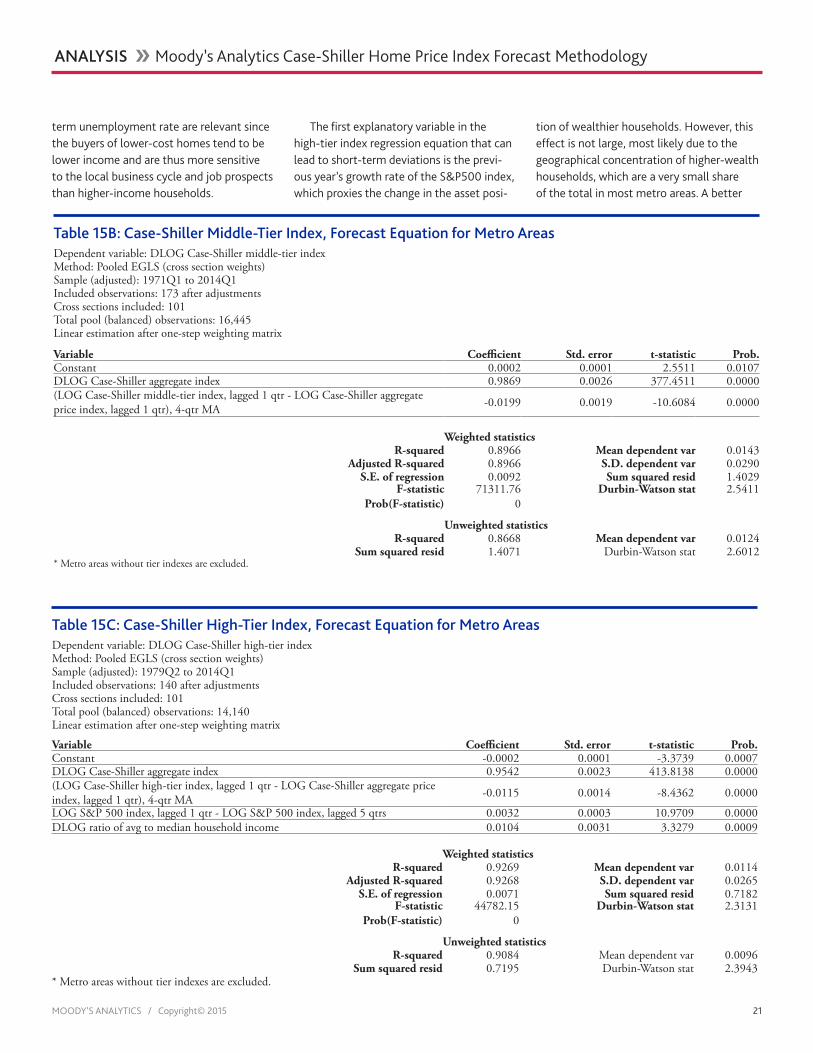
MOODY’S ANALYTICS / Copyright© 2015 21
ANALYSIS �� Moody’s Analytics Case-Shiller Home Price Index Forecast Methodology
Table 15B: Case-Shiller Middle-Tier Index, Forecast Equation for Metro AreasDependent variable: DLOG Case-Shiller middle-tier indexMethod: Pooled EGLS (cross section weights)Sample (adjusted): 1971Q1 to 2014Q1Included observations: 173 after adjustmentsCross sections included: 101Total pool (balanced) observations: 16,445Linear estimation after one-step weighting matrix
Variable Coefficient Std. error t-statistic Prob. Constant 0.0002 0.0001 2.5511 0.0107DLOG Case-Shiller aggregate index 0.9869 0.0026 377.4511 0.0000(LOG Case-Shiller middle-tier index, lagged 1 qtr - LOG Case-Shiller aggregate price index, lagged 1 qtr), 4-qtr MA -0.0199 0.0019 -10.6084 0.0000
Weighted statisticsR-squared 0.8966 Mean dependent var 0.0143
Adjusted R-squared 0.8966 S.D. dependent var 0.0290S.E. of regression 0.0092 Sum squared resid 1.4029
F-statistic 71311.76 Durbin-Watson stat 2.5411Prob(F-statistic) 0
Unweighted statisticsR-squared 0.8668 Mean dependent var 0.0124
Sum squared resid 1.4071 Durbin-Watson stat 2.6012* Metro areas without tier indexes are excluded.
term unemployment rate are relevant since the buyers of lower-cost homes tend to be lower income and are thus more sensitive to the local business cycle and job prospects than higher-income households.
The first explanatory variable in the high-tier index regression equation that can lead to short-term deviations is the previ-ous year’s growth rate of the S&P500 index, which proxies the change in the asset posi-
tion of wealthier households. However, this effect is not large, most likely due to the geographical concentration of higher-wealth households, which are a very small share of the total in most metro areas. A better
Table 15C: Case-Shiller High-Tier Index, Forecast Equation for Metro AreasDependent variable: DLOG Case-Shiller high-tier indexMethod: Pooled EGLS (cross section weights)Sample (adjusted): 1979Q2 to 2014Q1Included observations: 140 after adjustmentsCross sections included: 101Total pool (balanced) observations: 14,140Linear estimation after one-step weighting matrix
Variable Coefficient Std. error t-statistic Prob. Constant -0.0002 0.0001 -3.3739 0.0007DLOG Case-Shiller aggregate index 0.9542 0.0023 413.8138 0.0000(LOG Case-Shiller high-tier index, lagged 1 qtr - LOG Case-Shiller aggregate price index, lagged 1 qtr), 4-qtr MA -0.0115 0.0014 -8.4362 0.0000
LOG S&P 500 index, lagged 1 qtr - LOG S&P 500 index, lagged 5 qtrs 0.0032 0.0003 10.9709 0.0000DLOG ratio of avg to median household income 0.0104 0.0031 3.3279 0.0009
Weighted statisticsR-squared 0.9269 Mean dependent var 0.0114
Adjusted R-squared 0.9268 S.D. dependent var 0.0265S.E. of regression 0.0071 Sum squared resid 0.7182
F-statistic 44782.15 Durbin-Watson stat 2.3131Prob(F-statistic) 0
Unweighted statisticsR-squared 0.9084 Mean dependent var 0.0096
Sum squared resid 0.7195 Durbin-Watson stat 2.3943* Metro areas without tier indexes are excluded.

MOODY’S ANALYTICS / Copyright© 2015 22
ANALYSIS �� Moody’s Analytics Case-Shiller Home Price Index Forecast Methodology
explanatory variable is the ratio of average household income to median household income. The higher this ratio, the greater
the concentration of income among high-earning households and the greater the demand for more expensive homes. A 1%
increase in this share will cause the high-tier house price index to increase by about 0.1 percentage point.

MOODY’S ANALYTICS / Copyright© 2015 23
AUTHOR BIO �� www.economy.com
About the Authors
Celia ChenCelia Chen is a managing director of the Moody’s Analytics research staff, specializing in housing economics. Celia manages the Moody’s
Analytics regional house price forecast models, develops proprietary housing market indicators, and writes extensively about housing issues. Based in the West Chester PA office, Dr. Chen has participated in numerous consulting projects, including econometric modeling of regional house price forecasts, consumer lending, and mortgage lending.
Celia speaks regularly at Moody’s client conferences and has provided economic commentary for Bloomberg, CNBC and other media outlets. Celia completed her PhD at the University of Pennsylvania, with a concentration in econometrics and international finance. She holds a bachelor’s degree in economics from Barnard College.
Andres Carbacho-Burgos
Andres Carbacho-Burgos is a senior economist with Moody’s Analytics. He covers housing and state and regional economies, and writes frequently about inflation for Precis Macro from the company’s West Chester PA office. Before joining Moody’s Analytics, he taught economics at Texas State University, where he also researched open-economy macroeconomics and income inequality. He obtained his PhD and master’s degrees in economics from the University of Massachusetts at Amherst and his bachelor’s degree in economics from Carleton College.

© 2015 Moody’s Analytics, Inc. and/or its licensors and affi liates (together, “Moody’s”). All rights reserved. ALL INFORMATION CONTAINED HEREIN IS PROTECTED BY COPYRIGHT LAW AND NONE OF SUCH INFORMATION MAY BE COPIED OR OTHERWISE REPRODUCED, REPACKAGED, FURTHER TRANSMITTED, TRANSFERRED, DISSEMINATED, REDISTRIBUTED OR RESOLD, OR STORED FOR SUBSEQUENT USE FOR ANY PURPOSE, IN WHOLE OR IN PART, IN ANY FORM OR MANNER OR BY ANY MEANS WHATSOEVER, BY ANY PERSON WITHOUT MOODY’S PRIOR WRITTEN CONSENT. All information contained herein is obtained by Moody’s from sources believed by it to be accurate and reliable. Because of the possibility of human and mechanical error as well as other factors, however, all information contained herein is provided “AS IS” without warranty of any kind. Under no circumstances shall Moody’s have any liability to any person or entity for (a) any loss or damage in whole or in part caused by, resulting from, or relating to, any error (negligent or otherwise) or other circumstance or contingency within or outside the control of Moody’s or any of its directors, offi cers, employees or agents in connection with the procurement, collection, compilation, analysis, interpretation, communication, publication or delivery of any such information, or (b) any direct, indirect, special, consequential, compensatory or incidental damages whatsoever (including without limitation, lost profi ts), even if Moody’s is advised in advance of the possibility of such damages, resulting from the use of or inability to use, any such information. The fi nancial reporting, analysis, projections, observations, and other information contained herein are, and must be construed solely as, statements of opinion and not statements of fact or recommendations to purchase, sell, or hold any securities. NO WARRANTY, EXPRESS OR IMPLIED, AS TO THE ACCURACY, TIMELINESS, COMPLETENESS, MERCHANTABILITY OR FITNESS FOR ANY PARTICULAR PURPOSE OF ANY SUCH OPINION OR INFORMATION IS GIVEN OR MADE BY MOODY’S IN ANY FORM OR MANNER WHATSOEVER. Each opinion must be weighed solely as one factor in any investment decision made by or on behalf of any user of the information contained herein, and each such user must accordingly make its own study and evaluation prior to investing.
About Moody’s AnalyticsEconomic & Consumer Credit Analytics
Moody’s Analytics helps capital markets and credit risk management professionals worldwide respond to an evolving marketplace with confi dence. Through its team of economists, Moody’s Analytics is a leading independent provider of data, analysis, modeling and forecasts on national and regional economies, fi nancial markets, and credit risk.
Moody’s Analytics tracks and analyzes trends in consumer credit and spending, output and income, mortgage activity, population, central bank behavior, and prices. Our customized models, concise and timely reports, and one of the largest assembled fi nancial, economic and demographic databases support fi rms and policymakers in strategic planning, product and sales forecasting, credit risk and sensitivity management, and investment research. Our customers include multinational corporations, governments at all levels, central banks and fi nancial regulators, retailers, mutual funds, fi nancial institutions, utilities, residential and commercial real estate fi rms, insurance companies, and professional investors.
Our web periodicals and special publications cover every U.S. state and metropolitan area; countries throughout Europe, Asia and the Americas; the world’s major cities; and the U.S. housing market and other industries. From our offi ces in the U.S., the United Kingdom, the Czech Republic and Australia, we provide up-to-the-minute reporting and analysis on the world’s major economies.
Moody’s Analytics added Economy.com to its portfolio in 2005. Now called Economic & Consumer Credit Analytics, this arm is based in West Chester PA, a suburb of Philadelphia, with offi ces in London, Prague and Sydney. More information is available at www.economy.com.

ANALYSIS �� Moody’s Analytics Case-Shiller Home Price Index Forecast Methodology
Copyright © 2015, Moody’s Analytics, Inc. All Rights Reserved.
CONTACT US For further information contact us at a location below:
Email us: [email protected] visit us: www.economy.com
U.S./CANADA +1.866.275.3266
EMEA+44.20.7772.5454 London+420.224.222.929 Prague
ASIA/PACIFIC +852.3551.3077
OTHER LOCATIONS+1.610.235.5299