A Study of Coastal Flooding at Jarvis Creek, Connecticut

James O'Donnell, Michael Whitney and Kay Howard Strobel

Connecticut Institute for Resilience and Climate Adaptation

and

Department of Marine Sciences

University of Connecticut

August 29, 2016

 

i  

Table of Contents

Table of Contents List of Acronyms List of Figures Executive Summary 1. Introduction 2. Approach

2.1. Mathematical Model 2.2. Mapping the Basins 2.3. Mapping the Connections

3. Observation Campaign 4. Model Calibration 5. Analysis 6. Discussion and Conclusion 7. References

i

ii iii

1 2 5 5 7

12 15 19 21 22 25

  

ii  

List of Acronyms

CIRCA Connecticut Institute for Resilience and Climate Adaptation GPS Global Positioning System LISICOS Long Island Sound Integrate Coastal Observing System MLW Mean Low Water MSL Mean Slack Water NAVD88 North American Vertical Datum of 1988 NDEP National Digital Elevation Program NERACOOS Northeastern Regional Association of Coastal Ocean Observing Systems NOAA National Oceanic and Atmospheric Adminstration ODE23 Ordinary Diferential Equation solver RMSE Root Mean Square Error RTK GPS Real Time Kinematic Global Positionaing System UConn University of Connecticut

  

iii  

List of Figures

Page Figure 1. Google Earth© view of the Jarvis Creek Study area. The green

arrow shows where the Amtrak line between New York and Boston crosses the marsh. The causeway and bridge separate the northern basin from the central basin of the marsh system. The red arrow highlights the location of the tide gate that separates the southern basin of the creek from the central basin. A field in Medlyn’s Farm that is reported to be frequently flooded is shown by the orange arrow.

3

Figure 2. Photograph of the Amtrak railway causeway and bridge across Jarvis Creek marsh. The blue arrows indicate the width of the bridge and the yellow arrows show the raised causeway.

3

Figure 3. Aerial photograph of the Branford Trail where it crosses Jarvis Creek (from maps.bing.com; obtained between March-April 2011). On the eastern (right) side of the marsh the path is on a rock and earthen causeway (bounded by blue arrows) to the tide gate (green arrow). On the west (left) side of the marsh the trail crosses on to a timber bridge that was built above the location of the earthen berm that is indicated by the red arrows.

4

Figure 4. Topography and bathymetry of the Jarvis Creek marsh complex. The color scale on the right shows the elevation (positive) and depth below the NAVD88 vertical datum. The elevation in the areas shaded white was not recorded.

7

Figure 5. Google Earth© aerial photograph of the Jarvis Creek marsh complex. (a) shows two rectangles defining the locations of the higher resolution images shown in (b) and (c). The white circles show the locations of points where high precision GPS elevations were measured for checking the LIDAR elevations.

8

Figure 6. (a) Shows the gridded LIDAR topography in the area highlighted in Figure 5(c), together with the locations of the GPS survey locations, which are shown by the white squares and red * symbols. The latter are locations where the topography was relatively uniform and the LIDAR and GPS elevations were compared. In (b) the difference in the elevation estimates at the positions of the red * symbols are shown as a function of distance north. The error bars indicates ± 2 standard deviations (the 95% confidence interval) in the LIDAR estimates in the grid cell. The black line show the weighted mean of the errors. The solid red line shows the expected difference based on the NOAA (2005) and the dashed line shows the bounds of the 95% confidence interval.

9

  

iv  

Figure 7. The area of the northern basin of the Jarvis Creek marsh is identified by the light blue color and the central basin is identified by magenta. The color in the rest of the study area represents the topography. The scale is shown on the right.

11

Figure 8. The area of the water surface at different water elevations in (a) the northern basin, and (b) the central basin.

11

Figure 9. The variation of the volume to the two basins as a function of elevation. The northern basin is shown by the blue line and the central basin is shown in red.

12

Figure 10. (a) shows a Google Earth© view of the main channel of Jarvis Creek. The boundaries of the deepest parts of the channel are shown in green. Survey point as identified by numbers and the depth below mean low water are shown in (b). The photographs in (c) and (d) show the Amtrak bridge crossing Jarvis Creek at low water.

13

Figure 11. The simplified representation of the channel cross-section at the Amtrak Bridge across Jarvis Creek.

13

Figure 12. The simplified representation of the channel cross-section at the tide gate. The top of the gate is at -1.1 m NAVD88.

14

Figure 13. Options for the model representation of the earthen berm cross-section on the marsh to the west of the tide gate. (a) Shows the current situation and (b) show a more restrictive configuration to simulate the conditions prior to the construction of the walkway.

14

Figure 14. Google Earth© photograph of Jarvis Creek showing the locations of the three Level Logger pressure sensors at the sits labeled LL1, LL2 and LL3, and the four instrument frames at F1, F2, F3 and F4.

15

Figure 15. Photographs of (a) the MicroCAT (left) and Aquadopp (right) deployed at F1 and F3; (b) the MicroCAT deployed at F2 and F3; and (c) the Level Logger deployed at LL1-3.

16

Figure 16. Meteorological Observations at the CLIS buoy: (a) wind speed (knots), (b) wind directions (degrees), (c) surface air pressure (mBar), and (d) air temperature (Celsius). The clouds at the top of the figure indicate days when there was significant rain.

17

Figure 17. (a) Water level measured at LL1 (red), LL2 (blue) and LL3 (green) in Jarvis Creek in the winter of 2014. (b) shows the data from Nov. 22 to Nov 26 in higher resolution. Locations are shown in Figure 14. The yellow band shows the level of RT 146 where it crosses the

18

  

v  

northern boundary of the marsh complex. The dashed lines indicate periods when the road was reported to be flooded.

Figure 18. The evolution of the water levels at LL1 and LL3 (a) and the

correlation between LL1 and LL3, r^2 (τ), as a function of lag (hrs). The maximum correlation is at lag of 45 minutes.

19

Figure 19. The evolution of the water levels at LL2 and LL3 (a) and the correlation between LL2 and LL3, r^2 (τ), as a function of lag (hrs). The maximum correlation is at lag of 15 minutes.

19

Figure 20. Comparison of the observations of water level at LL1 (blue), LL2 and LL3 (grey), and the simulations at LL2 (green), and LL3 (red).

20

Figure 21. Comparison of the observations of water level at LL1 (blue), LL2 and LL3 (grey), and the simulations at LL2 (green), and LL3 (red) when the earthen berm is replaced by a wall that prohibits flow over the marsh.

21

Figure 22. Comparison of the observations of water level at LL1 (blue), LL2 and LL3 (grey), and the simulations at LL2 (green), and LL3 (red) when the earthen berm configuration shown in Figure 13(b) is employed.

22

Figure 23. Time series of the difference between model predictions at LL3 when water is allowed to flow through the marsh and berm (shown in Figure 20), and when it is not (Figure 22).

23

 

1  

Executive Summary

The Town of Branford, CT, and the Branford Land Trust have reported that high water levels at Jarvis Creek Marsh, CT, have led to flooding on Leetes Island Road (RT 146) and at a field adjacent to the marsh. Exchange of water between Long Island Sound and the marsh complex is currently influenced by a tide gate and a berm at the southern end of marsh and a railway bridge that crosses the middle of the marsh. The berm had been modified by the Land Trust with funds from a grant from the Connecticut Department of Energy and Environmental Protection as part of a marsh restoration program and to improve public access. This report describes observation and the development of a mathematical model that quantitatively assesses the influence of the tide gate and the berm on the exchange with Long Island Sound and the frequency of flooding.

We deployed an array of water level, salinity, and current sensors at 8 locations in the study area between October 18th and December 28th, 2014 to observe the water level changes in a wide variety of wind and tidal conditions. We also created a gridded topography and bathymetry of the marsh complex using LIDAR and several GPS surveys to ensure that the water level measurements were referenced to a geodetic datum. We also carefully measured the geometry and water depth at the tide gate, the berm and the railway bridge. These data were used to develop and evaluate a mathematical model to link the fluctuations of water level in Long Island Sound to the mean level in the marsh north of the railway bridge.

With the best representation of the current geometry of the berm we demonstrated that the model reproduced the fluctuations observed in the upper portion of Jarvis Creek Marsh with an error in the prediction of high water of approximately 10 cm. Both observations and the model showed that the rail line crossing had no effect on the high water levels, though it did raise the level at low tide. We then used the model to assess what the water level would have been in 2014 had the berm not been substantially modified. We also simulated the effectiveness of a berm that did not permit any flow around the tide gate. We found that the effect of removing the entire berm was to decrease the high water level by approximately 10 cm and that the consequences of a more effective berm were essentially the same. This magnitude is comparable to that of the expected error in the model predictions.

We conclude that the presence (or absence) of the berm had little effect on the water levels or the occurrence of flooding at RT 146. The flow is controlled by the tide gate. If the tide gate were substantially modified, then the importance of the berm should be reassessed.

  

2  

1. Introduction

The coastline of Connecticut was sculpted by continental-scale tectonic forces and multiple glaciations. It has been modified extensively in the last 10,000 years by the consequences of rising sea level and the transport of sediment by rivers and tidal currents. These processes have led to the heterogeneous coastal landscape that both residents and tourists value. Tidal marsh complexes are common and important elements of the regional ecosystem. They form in embayments that are generally sheltered from the energetic waves and currents of Long Island Sound and they are found in all of Connecticut’s shoreline municipalities. Important local and state roads between population centers often skirt the northern edges of these marshes. In the last century the population density of the shoreline has increased and many of the coastal marshes are now surrounded by homes and businesses. In many places marshes have been filled to accommodate additional development.

The flow of water between the tidal marshes and Long Island Sound is generally constrained by rocky headlands and sandy spits. These are important elements of the recipe for marsh formation. However, to manage the frequency of flooding, and shorten road and train routes, additional flow constrictions have been introduced into Connecticut’s marshes. They include tide gates, culverts beneath roads and rail lines, and bridges. These structures are important to the determination of the frequency and extent of flooding in many areas of Connecticut.

To understand the likely effects of the future sea level rise on flooding of roads and buildings in Connecticut’s towns, we need to quantitatively understand the changes to the statistics of sea level variations in the ocean and Sound, and the flow of water through marsh systems. The Connecticut Institute for Resilience and Climate Adaptation (CIRCA) is undertaking research projects to enable more accurate flood risk assessment. The opportunity to develop and evaluate an approach to represent the effects of small-scale constrictions like tide gates and bridges on flooding in areas surrounding a marsh is of great value.

The Town of Branford (http://www.branford-ct.gov/) and the Branford Land Trust (http://branfordlandtrust.org/) are concerned about flooding that frequently occurs on Leetes Island Road (RT 146) and the surrounding properties through Jarvis Creek, a tidal marsh complex that is connected to Long Island Sound. Figure 1 shows a map of the study area. The yellow line shows Leetes Island Road skirting the northern edge of the marsh. The Amtrak train line between New York and Boston crosses Jarvis Creek at the location shown by the green arrow in Figure 1. The line crosses the marsh on a raised causeway and bridge. Figure 2 shows a photograph of the railway from the south with the limits of the causeway shown by the yellow arrows and the extent of the bridge indicated by the blue arrows. The causeway and bridge limit water transport between the northern and central sections of the marsh. We term the area to the north of the Amtrak line the “northern basin”.

  

3  

Figure 1. Google Earth© view of the Jarvis Creek Study area. The green arrow shows where the Amtrak line between New York and Boston crosses the marsh. The causeway and bridge separate the northern basin from the central basin of the marsh system. The red arrow highlights the location of the tide gate that separates the southern basin of the creek from the central basin. A field in Medlyn’s Farm that is reported to be frequently flooded is shown by the orange arrow.

 

 

Figure 2. Photograph of the Amtrak railway causeway and bridge across Jarvis Creek marsh. The blue arrows indicate the width of the bridge and the yellow arrows show the raised causeway.

The red and blue arrows on Figure 1 show the location of the Branford Trail, a hiking pathway across the marsh. The eastern part of the trail rests on what appears to be a rock and earthen

Medlyn’s 

Field 

Amtrak 

  

4  

causeway which leads to the concrete support structure for a wooden tide gate. This is shown in the aerial photograph in Figure 3. The image was obtained between March and April 2011, and published by maps.bing.com. Note that the date of the image is not made available by the bing.com viewer, it was instead obtained using http://mvexel.dev.openstreetmap.org/bing/.

The blue arrows show the pathway to the tide gate, which is indicated by the green arrow. To the west (left in the picture) of the tide gate the trail rests on a low earthen berm that is bounded by red arrows in the Figure. At the time of the picture the elevated walkway that is now in place had not been constructed. The causeway, tide gate, and berm combine to restrict the exchange of water between the central basin of the marsh complex and the southern basin.

 

Figure 3. Aerial photograph of the Branford Trail where it crosses Jarvis Creek (from maps.bing.com; obtained between March-April 2011). On the eastern (right) side of the marsh the path is on a rock and earthen causeway (bounded by blue arrows) to the tide gate (green arrow). On the west (left) side of the marsh the trail crosses on to a timber bridge that was built above the location of the earthen berm that is indicated by the red arrows.

The central goal of this study is to assess the relative importance of the tide gate, earthen berm and the railway bridge on the water levels in the northern basin where frequent flooding of Leetes Island Road (RT 146) and the adjacent properties (e.g. a field that is part of Medlyn’s Farm, see Figure 1) has been reported. The berm had been modified by the Land Trust as part of a marsh restoration project and to improve public access using funds obtained from a third party through an enforcement action taken by the Connecticut Department of Energy and Environmental Protection. It is of interest to assess the potential consequences of the change on

Causeway 

to tide gate 

Tide gate

Earthen berm 

  

5  

water levels. This area provides a convenient study site for examining the effectiveness of simple models of the effect of flow constrictions on marsh flooding. Issues such as this are likely to arise more frequently in the future as sea level rise increases the frequency of coastal flooding. This site also has the advantage of leveraging the collaboration of Prof. Peter Raymond (Yale University) and his students who have been supported by the Town of Branford which purchased, and made available, water level and salinity sensors to augment the instruments deployed by UConn. Valuable assistance in mapping was provided by students from Branford High School.

2. Approach

To quantify the effects of the exchange between the Long Island Sound and the three basins of the Jarvis Creek marsh complex, we developed a simple hydraulic model of water exchange following the approach developed by Roman et al. (1995). This approach was originally developed to assess the effects of the removal of tide gates at the mouth of the Herring River, MA, on flooding at the head of the river. The model represents the marsh complex mathematically as a network of basins with known area and hypsometry linked by short connectors that are characterized by their width, and depth and a frictional dissipation parameter. The geometry used in the model is established by mapping the topography and bathymetry. Parameter values are estimated by “fitting” model predictions to measurement of the fluctuations of water levels through a wide range of conditions. With this information, the model can be used to evaluate the relative importance of the various constrictions on the sea levels of each basin. Note that the sea level within each of the three basins is assumed to be flat. This is a good assumption since the basins are small.

2.1 Mathematical Model

The principle that the rate of change of the volume of water in the northern basin, , with time, ,is equal to the rate at which it enters from the upland source (a small stream) minus the rate at

which it drains to the central basin through the constriction formed by the Amtrak bridge can be expressed mathematically as

, ,

(1)

where the symbols and , represent the flow rates into, and out of, the basin. Note that

depends upon the bathymetry of the basin and the water level .Since the water level in the central basin, ,can be higher or lower than that in the northern basin, , the flux , can be

either positive or negative. The well-established Manning Formula (Linsley and Franzini, 1979) is used to relate the flow rate to the sea level difference as

  

6  

,,

, ,

| |

, | |,

(2)

where , and , are the cross sectional area and length of the flow constriction, , is the

“wetted perimeter”, the length of the intersection between the water and rigid boundary in the cross-sectional plane. The friction parameter is , and is referred to as the Manning

coefficient. Note that the sign of , is positive when , i.e. the flow is out of the basin.

It is also important to note that the cross section and wetted perimeter vary with the water levels: i.e. , , , , and , , , .

The analogous water volume budget for the central basin is expressed as

, ,

(3)

where the exchange with the southern basin takes place through both the tide gate, , and the earthen berm, . Both of these are again expressed in terms of the difference in the water levels between the central and southern basins using Manning’s formula as

| |

| |

(4)

and

| |

| |

(5)

This system of two non-linear ordinary differential equations, Equations (1) and (3), is forced by prescribed variations in the water level in the southern basin, ,and the solution yields the evolution of the two unknown functions, the water levels and . The areas [ , , , , ,and , and wetted perimeter [ , , , , ,and , ] parameters vary with the water levels and these dependences, together with the constriction lengths [ , , , and ], must be prescribed by measurement. The Manning

coefficients [ , , , and ] can be estimated using literature values and refined by a

systematic calibration procedure which minimizes the differences between the measurements and predictions of and .

The complexity of the equations requires that numerical methods be employed. The differential equations were solved using the programming and computing environment MATLAB© and the ordinary differential equation solver ODE23. Changes in the basin areas with elevations were prescribed using an analysis of LIDAR elevation data (see section 2.2). The river source ( was estimated using discharge measurements at Indian River (USGS gauge 1195100) and

  

7  

multiplying the series by the ratio of the watershed areas. This procedure worked effectively and efficiently.

2.2 Mapping the Basins

To prescribe how the water level in the basins is linked to the volumes, i.e. prescribing and ,the topography of the study area must be established. This was accomplished using data from the NOAA LIDAR elevation library. This data was median averaged in 5 525 , square intervals and the resulting topography-bathymetry is shown in Figure 4. The axes show distance east and north from the location 72 o 44.9’ E, 41o 15.6’ N. The broad areas shown in blue are the almost level marshes surfaces. The level of RT 146 is clear on the right side of Figure 4 is the almost straight yellow line (highlighted by left pointing arrow). The Amtrak line is represented by the downward sloping red line in the middle of Figure 4 (highlighted by the right pointing arrow).

 

Figure 4. Topography and bathymetry of the Jarvis Creek marsh complex. The color scale on the right shows the elevation (positive) and depth below the NAVD88 vertical datum. The elevation in the areas shaded white was not recorded.

To establish the uncertainty in the LIDAR topography, we acquired independent elevation measurements using an RTK GPS surveying system. Figure 5 shows an aerial photograph (Google Earth©) with white circles indicating the location of the GPS elevation estimates that we

Distance east (m)

Distance north (m) 

  

8  

acquired. The LIDAR data acquisition (NOAA, 2005) was accompanied by ground surveys at 30 points near the Connecticut shoreline that were selected to be clear of vegetation and level. The comparison between the three closest LIDAR estimates interpolated to the survey points showed that the mean error in elevation was 0.05m, with a standard deviation of 0.04m. The largest difference was 0.12m. As is clear in Figure 5, our GPS survey contained a variety of site conditions. Most were on the marsh surface, but some were near the edge of the marsh and on the structures.  

 

Figure 5. Google Earth© aerial photograph of the Jarvis Creek marsh complex. (a) shows two rectangles defining the locations of the higher resolution images shown in (b) and (c). The white circles show the locations of points where high precision GPS elevations were measured for checking the LIDAR elevations.

To assess the consistency of the GPS and LIDAR area average elevations we compared the GPS elevation estimate to the average at the cell containing the surveyed point. To be clear, we defined the error as the GPS value minus the LIDAR estimate, i.e. , which is consistent with the definitions in the report evaluating the accuracy of Connecticut Coastal LIDAR survey reported by NOAA (2005). Note that this is opposite in sign to the definition recommended by NDEP (2004). To control for the effects of variations in level across the averaging interval, we restricted comparisons to cells where the standard deviation of LIDAR

(a)  (b) 

(c) 

  

9  

estimates was less than 0.1m. These points were largely on the surface of the marsh. Figure 6(a) shows the elevation of the marsh in the vicinity of the berm (see Figure 5(c)) and the locations of GPS survey points where the standard deviation of the LIDAR estimates in the coincident grid cell was less than 0.1m are shown by the red * symbols. The variation of the values of at these points is presented in Figure 6(b) with distance north shown in Figure 6(b). The error bars represent 2 standard deviations in the LIDAR estimates contributing to the mean. The solid black line shows that the mean error is -0.1m, or that the LIDAR values are 0.1m higher than expected. In contrast, the NOAA (2005) report suggested that the mean error would be 0.05m. This level is shown by the solid red line in Figure 6(b) and the 2 standard deviation interval is bounded by the red dashed lines.

Figure 6. (a) Shows the gridded LIDAR topography in the area highlighted in Figure 5(c), together with the locations of the GPS survey locations, which are shown by the white squares and red * symbols. The latter are locations where the topography was relatively uniform and the LIDAR and GPS elevations were compared. In (b) the difference in the elevation estimates at the positions of the red * symbols are shown as a function of distance north. The error bars indicates 2 standard deviations (the 95% confidence interval) in the LIDAR estimates in the grid cell. The black line show the weighted mean of the errors. The solid red line shows the expected difference based on the NOAA (2005) and the dashed line shows the bounds of the 95% confidence interval.

The bias in the LIDAR estimates of the level of the marsh relative to our GPS estimates is 0.1m. Assuming the original calibration to the “bare earth” sites of NOAA (2005) is applicable in our study area, then the marsh surface level estimates are biased 0.15m high. Results in other areas

  

10  

of the Jarvis Creek marsh surface show the same results. This magnitude is not inconsistent with the height of the marsh vegetation. Recently, McClure et al. (2015) has demonstrated that in a marsh system in California, the LIDAR elevations had to be reduced by between 0.10 and 0.25 m to remove the effects of different marsh grass species on the elevation levels.

The rate of change of volume with time in Equations (1) and (3) can be written as

which is equivalently . To establish how the volume of water in each

basin varies with the water level, the gridded topography in Figure 4 was separated into the region north of the Amtrak line ( ), and the region between the Amtrak line and the causeway-tide gate ( ). The areas below the 3m elevation contour in basins 1 and 2 are shaded light blue and magenta respectively in Figure 7. The number of grid cells in basins 1 and 2 below the level

are denoted and ,and these were evaluated using a simple constrained search for

2 /5 and 1to 30. Since the area of each cell is 25 , the area of the basin at each elevation is simply , 25 , . Figure 8 shows and .

Figure 8 (a) and (b) show that the variation of the marsh with altitude is similar in each basin. The graphs show that the surface area of the marsh increases by approximately a factor of 1000 between -0.5 and 0.6 m elevation (NAVD88). Above 0.6 m the basin is much more constrained by the steep edge of the uplands and the area does not change much. Though they are not central to the calculations, the volume of each basin below level can be computed as

5∑ , and 5∑ and these functions are shown in Figure 9.

  

11  

 

Figure 7. The area of the northern basin of the Jarvis Creek marsh is identified by the light blue color and the central basin is identified by magenta. The color in the rest of the study area represents the topography. The scale is shown on the right.

 

Figure 8. The area of the water surface at different water elevations in (a) the northern basin, and (b) the central basin.

(a)  (b) 

Distance east (m)

Distance north (m) 

  

12  

 

Figure 9. The variation of the volume to the two basins as a function of elevation. The northern basin is shown by the blue line and the central basin is shown in red.

2.3 Mapping the Connections

In the model, the northern basin has two sources of water, a small stream and the connection to the central basin. The streamflow is minor and was estimated from the measured flow rate and the ratio of the areas of the watersheds. The geometry of the connections between the basins is important in the parameterization of the exchange between the basins in Equations (2), (4) and (5). Figure 10(a) shows a Google Earth© aerial photograph of the main channel of Jarvis Creek with the boundaries of the deepest parts of the channel shown in green and survey points identified by numbers. The depth at these points is shown in Figure 10(b). The level of the channel bottom is approximately -0.5m relative to Mean Low Water (MLW) in much of the central basin, though it is much deeper to the south of the bridge. Note that the NOAA tidal gage at Branford River (https://tidesandcurrents.noaa.gov/benchmarks/8465233.html) indicates that MLW is at -0.97m relative to the NAVD88 datum. A photograph of the Amtrak Bridge looking to the north is shown in Figure 10(c). The sides of the section under the bridge are vertical. However, under the bridge the bottom of the channel is rocky and slopes down from the sides to the center of the channel. Figure 10(d) shows a close up of the flow in to the central basin at low tide. We measured the width of the connection as 20.8 m, and the depth of the channel at the center as 0.75 below MLW or -1.72 m NAVD88. The length of the channel, , , was measured

as 40m. We approximate the section geometry as a triangle as shown in Figure 11 and used this to compute , and , .

  

13  

 

Figure 10. (a) shows a Google Earth© view of the main channel of Jarvis Creek. The boundaries of the deepest parts of the channel are shown in green. Survey point as identified by numbers and the depth below mean low water are shown in (b). The photographs in (c) and (d) show the Amtrak bridge crossing Jarvis Creek at low water.

 

Figure 11. The simplified representation of the channel cross-section at the Amtrak Bridge across Jarvis Creek.

The rectangular connection at the tide gate was measured to be 3.66m wide. The elevation of the concrete tide gate structure was measured by GPS (and was within 1 cm of the LIDAR level estimate) as 2.32 m above NAVD88. The level of the sill was measured manually as 3.42 m below that at -1.1m relative to NAVD88. This is shown schematically in Figure 12 and these

(a) 

(b) 

(c) 

(d) 

  

14  

values were used to prescribe and in Equation (4). The length of the constriction was set as 30m to represent the effects of the whole tide gate structure.

 

Figure 12. The simplified representation of the channel cross-section at the tide gate. The top of the gate is at -1.1 m NAVD88.

The second connection between the central basin and Long Island Sound in the model represents the over-marsh flow through/over the earthen berm and under the walkway to the west of the tide gate. The elevation of the marsh surface in the vicinity of the berm averaged 0.59 m above NAVD88. The current rocks-gravel path is approximately 0.20 m above that, so the berm was defined to be 0.79 m above NAVD88, 0.87 m above MSL, or 1.76 m above MLW. This is shown in Figure 13 (a). Note that the width of the gap was estimated as 39.3m which is the narrowest part of the gap between the highlands to the west of the marsh and the tide gate structure. Photographs of the berm before the construction of the walkway showed that it had been higher, though storms created two major gaps. Based on photographs we estimated that the former level was 0.61 m higher and that the gaps were 25% of the width as is shown schematically in Figure 13 (b). The length of the restriction was defined as 30m.

 

Figure 13. Options for the model representation of the earthen berm cross-section on the marsh to the west of the tide gate. (a) Shows the current situation and (b) show a more restrictive configuration to simulate the conditions prior to the construction of the walkway.

  

15  

3. Observation Campaign

To estimate the friction coefficients in Equations (2), (4) and (5), we deployed instruments to measure sea level variations at the sites shown in Figure 13. Two instrument frames with SeaBird Instruments MicroCAT SBE37’s (to measure pressure, temperature and salinity), and a Nortek AQD (to measure pressure, temperature and current velocity) were deployed at the sites labeled F1 and F3 in Figure 13. A photograph of the instruments prior to deployment is shown in Figure 14(a). Two additional frames with SBE37’s were also deployed at sites F2 and F4 and a photograph of the frame is shown in Figure 14(b). Three Solinst Level-Loggers were deployed to measure water level at the sites labeled LL1, LL2 and LL3 in Figure 13 and these are shown in Figure 14(c). The instruments were deployed between Oct. 24 and Dec. 29, 2014, a time of the year when the wind speeds and wind induced sea level fluctuations are generally energetic. All instruments worked as anticipated, with the exception of the Aquadopp at F1, which appears to have either been deployed at a high tilt/roll angle, or to have had a malfunction in the sensors.

 

Figure 14. Google Earth© photograph of Jarvis Creek showing the locations of the three Level Logger pressure sensors at the sits labeled LL1, LL2 and LL3, and the four instrument frames at F1, F2, F3 and F4.

  

16  

Figure 15. Photographs of (a) the MicroCAT (left) and Aquadopp (right) deployed at F1 and F3; (b) the MicroCAT deployed at F2 and F3; and (c) the Level Logger deployed at LL1-3.

Meteorological conditions in the area are routinely measured by the NERACOOS-LISICOS buoy (http://lisicos.uconn.edu/about_clis.php) in central Long Island Sound. The wind speed record is shown in Figure 16 (a). The red line shows the series of the maximum speed in 15-minute intervals and the blue line shows the interval mean. As is typical in the area during the late fall and early winter, periods of strong winds (exceeding 15 knots) occur almost every week. The direction the wind is coming from is shown in Figure16 (b), the surface air pressure and temperature are shown in Figures 16 (c) and (d) to demonstrate that high wind speed periods are associated with low pressure, cold temperatures, and winds from the northwest (270 o -360o).

Table 1 lists dates when flooding was reported on RT 146 at Jarvis Creek. These intervals are shown in Figure 16 (a) by the blue clouds. The variation of water level at LL1, LL2 and LL3 relative to MSL are shown in Figure 17 with flooding intervals bracketed by the vertical dashed lines. The red line shows the variations at LL1 at the southern end of the marsh. The green line show the level at LL3 at the northern end of the system. The blue lines show the level in the central basin, between the Amtrak Bridge and the tide gate. Close inspection of the series in Figure 17 (b) shows that the maxima in the LL1 series (near the Sound) are larger than the levels in the marsh. The maxima at LL2 and LL3, however, are very similar though the minima at LL3 are approximately 0.1 m higher than at LL2, and 0.3 m above those at LL1. It appears that both the tide gate and the Amtrak Bridge raise the water level at low tide, relative to the LL1, but only the tide gate has an effect on the level of high water.

Table 1. Periods when road flooding was reported during the observation campaign.

Date DescriptionOct 31-Nov 1 Road flooding November 6 Rain storm, road flooding November 24 Rain event, road flooding December 5-6 Rain event, road flooding December 9 Road flooding

December 25 Rain Event, Road flooding

  

17  

 

Figure 16. Meteorological Observations at the CLIS buoy: (a) wind speed (knots), (b) wind directions (degrees), (c) surface air pressure (mBar), and (d) air temperature (Celsius). The clouds at the top of the figure indicate days when there was significant rain.

 

The elevation of RT 146 in the area that it crosses the northern edge of Jarvis Creek was measured using GPS as between 0.81 and 1.05 m above NAVD88, or 0.89 to 1.13 m above MSL (using the Branford River water level gage as reference). In Figure 17 (a) and (b) this interval is shaded in yellow. Though there are many periods when the water level at LL1 crosses into the yellow band, there are seven occasions when the LL3 level (green symbols) exceeds the 0.89 m level. Five of these occur when road flooding was observed. It is likely that it also occurred during the other two periods, but was unreported.

The constrictions at the tide gate clearly reduce the level of the high water, however, the relationship between the level at LL3 and LL1 is nonlinear. Figure 18 (a) shows the relationship between the elevation at LL1 and LL3 more clearly. If the levels were identical, then points would all fall on the diagonal black line in the graph. A fractional reduction in the level at LL1 would result in a straight line at a shallower angle and a constant time lag in the response at LL3 would cause the points to form an ellipse. The observed departure from the diagonal is a consequence of both an amplitude reduction and a variable time lag at LL3 which is introduced

  

18  

by the constrictions that inhibit the flow. Figure 18 (b) show the lagged correlation function. The maximum occurs when LL1 is lagged by 45 minutes, which is the average lag.

 

Figure 17. (a) Water level measured at LL1 (red), LL2 (blue) and LL3 (green) in Jarvis Creek in the winter of 2014. (b) shows the data from Nov. 22 to Nov 26 in higher resolution. Locations are shown in Figure 14. The yellow band shows the level of RT 146 where it crosses the northern boundary of the marsh complex. The dashed lines indicate periods when the road was reported to be flooded.

Figure 19 (a) shows the relationship between the water levels at LL2 (in the central basin) and LL3 (in the northern basin). That the red points largely fall on the black diagonal line indicates that the effect of the flow restriction at the Amtrak Bridge is very modest. The cloud of red points broadens when fluctuations at LL2 are negative which shows that when the water depth at the bridge is shallow, there is a more significant impact on the flow draining from the northern basin. The lagged correlation diagram in Figure 19(b) show that the maximum occurs at a much

(a) 

(b) 

  

19  

smaller lag (15 minutes) than in Figure 18(b). In summary, the water level data suggests that the flow restrictions at the tide gate are the dominant control of water level throughout the marsh.

 

Figure 18. The evolution of the water levels at LL1 and LL3 (a) and the correlation between LL1 and LL3, , as a function of lag (hrs). The maximum correlation is at lag of 45 minutes.

 

Figure 19. The evolution of the water levels at LL2 and LL3 (a) and the correlation between LL2 and LL3, , as a function of lag (hrs). The maximum correlation is at lag of 15 minutes. 

4. Model Calibration

To estimate the Manning coefficient, , , in Equation (2), the parameter determining the

magnitude of frictional effects at the Amtrak Bridge, we prescribed in Equation (2) using the observations of elevation at LL2 and the geometric parameters shown in Figures 9 and 11, and then solved for numerically. We then compared the solution to the data obtained at LL3 and computed the root mean square error (RMSE). Using a simplex search algorithm we

(b) (a) 

(a)  (b) 

  

20  

systematically adjusted the parameter value and obtained , 0.04 as the value that

minimized the RMSE. We then included the central basin in the model by solving Equations (1)-(5) simultaneously for and with , 0.04, the tide gate geometry shown in Figure 12

and the current situation berm configuration shown in Figure 13(a), and the elevation data from LL1 to prescribe . We then iterated to obtain the values of and  that minimized the difference between and the data at LL2. The procedure yielded 0.06.

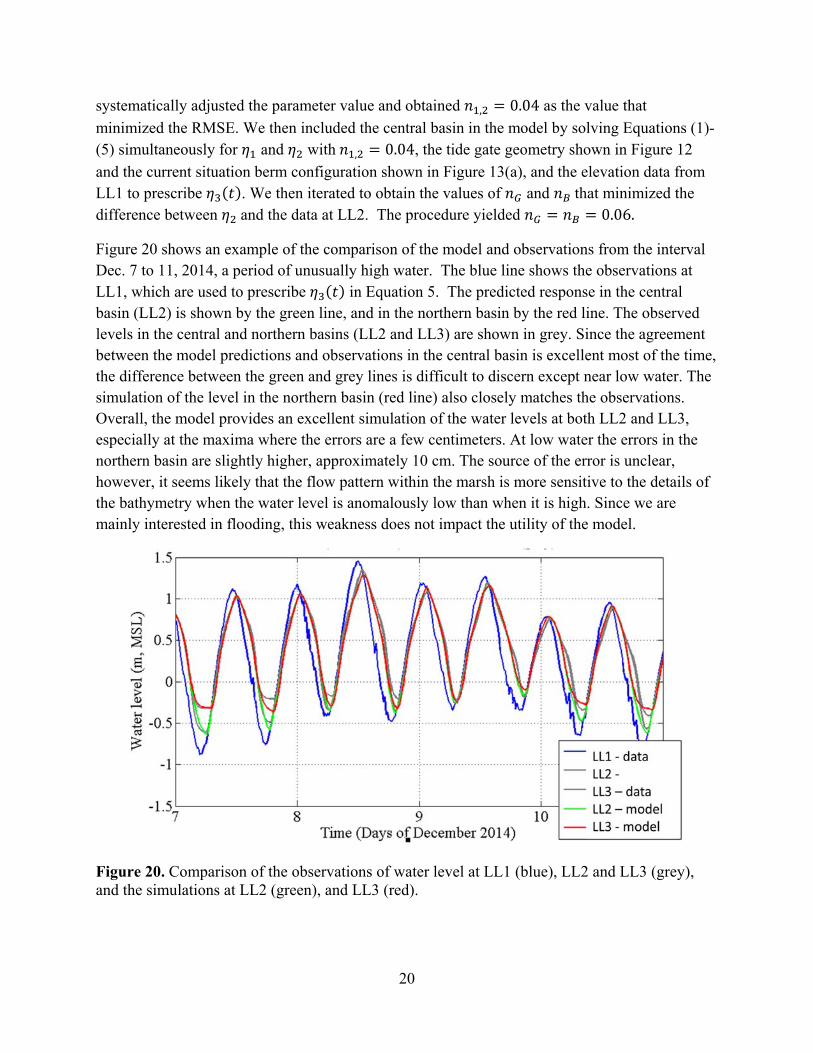
Figure 20 shows an example of the comparison of the model and observations from the interval Dec. 7 to 11, 2014, a period of unusually high water. The blue line shows the observations at LL1, which are used to prescribe in Equation 5. The predicted response in the central basin (LL2) is shown by the green line, and in the northern basin by the red line. The observed levels in the central and northern basins (LL2 and LL3) are shown in grey. Since the agreement between the model predictions and observations in the central basin is excellent most of the time, the difference between the green and grey lines is difficult to discern except near low water. The simulation of the level in the northern basin (red line) also closely matches the observations. Overall, the model provides an excellent simulation of the water levels at both LL2 and LL3, especially at the maxima where the errors are a few centimeters. At low water the errors in the northern basin are slightly higher, approximately 10 cm. The source of the error is unclear, however, it seems likely that the flow pattern within the marsh is more sensitive to the details of the bathymetry when the water level is anomalously low than when it is high. Since we are mainly interested in flooding, this weakness does not impact the utility of the model.

 

Figure 20. Comparison of the observations of water level at LL1 (blue), LL2 and LL3 (grey), and the simulations at LL2 (green), and LL3 (red).

  

21  

5. Analysis

To assess the relative importance of the tide gate and the flow over the marsh and earthen berm we set the term 0 in Equation (3). Conceptually, this is equivalent to replacing the marsh and berm with an impenetrable wall since no flow is allowed irrespective of the water levels. Figure 21 shown the observations and the solution to this version of the model for the same interval shown in Figure 20. The differences in the predicted water levels are imperceptible. Since the flow over the berm only has an effect when the water levels exceed 0.87 m relative to MSL differences in the model solutions should be restricted to the five highest peaks in Figure 21. However, though the depth of the flow over the berm is initially small, the wetted perimeter,

in Equation (5), is large. Since the flux over the berm, , is inversely proportional to , the magnitude is always small relative to the flow through the tide gate.

 

Figure 21. Comparison of the observations of water level at LL1 (blue), LL2 and LL3 (grey), and the simulations at LL2 (green), and LL3 (red) when the earthen berm is replaced by a wall that prohibits flow over the marsh.

To estimate the effect of berm geometry prior to the project that constructed the walkway (a higher, partially breached earthen berm), we repeated the simulation using the berm geometry shown in Figure 13(b). The results are presented in Figure 22. As expected, it is difficult to discriminate differences from the original simulation shown in Figure 20. To clarify the effect of the larger berm, we plot in Figure 23 the differences between the solution at LL3 in Figures 20 and 22. Positive values indicate the smaller berm has higher predicted sea level. Figure 23 demonstrates that the largest effects occur just after high tide during flood periods. The negative spikes have an amplitude of approximately 10 cm. This result implies that the removal of the

  

22  

berm slightly reduced the level of the water during the December 8th flooding event for a very short time. This is due to the slight change in the difference in the levels between LL1 and LL2 that occurs when water is allowed to flow over the marsh. The magnitude of this effect is quite small however and not much different from the difference between the model predictions and the observations. We conclude that the effect of the modification to the berm associated with the construction of the walkway has no detectable impact on the level of the water in the northern part of the marsh.

 

Figure 22. Comparison of the observations of water level at LL1 (blue), LL2 and LL3 (grey), and the simulations at LL2 (green), and LL3 (red) when the earthen berm configuration shown in Figure 13(b) is employed.

6. Discussion and Conclusions

The mathematical model we have developed and analyzed is a simplification of all the processes that are operating in nature. Several assumptions and approximations have been made. The net effect of these can be assessed by comparing the model predictions and observations shown in Figure 20. The errors in the predictions of the high water levels at LL3 are less than 5 cm. The model is generally biased high by approximately10 cm when compared to the observations of the water level at low tide. This is likely due to errors in the specification of the bathymetry of the basins at low water levels. The variation in the marsh vegetation species and elevation may lead to a 10 cm change in level for example.

  

23  

These errors set the sensitivity of the model. Changes in the configuration of the geometry of the flow constrictions would lead to changes of significantly more than 10 cm before it could be confidently concluded that they had an effect. Our analysis demonstrates that the modification of the berm at Jarvis Creek did not have a detectable impact on the water levels in the northern basin or change the flooding frequency on RT 146.

 

Figure 23. Time series of the difference between model predictions at LL3 when water is allowed to flow through the marsh and berm (shown in Figure 20), and when it is not (Figure 22).

An important goal of this study was to provide advice on how studies of marsh and road flooding should be conducted. The effectiveness of the model in simulating the observations (Figure 20) and the correspondence between the surveyed road level, water levels, and the occurrence of flooding (Figure 17) leads us to conclude that the general approach and deployment duration is adequate. However, the recent work of McClure et al. (2015) suggest that the determination of basin geometry using available LIDAR measurements should carefully consider errors associated with changing marsh flora elevations and distributions. Secondly, we have used water level datums from a nearby tide station to link our measurements to the NAVD88 datum. It would have been better to have surveyed the level that the sensors were deployed directly. This could be accomplished in the shallow areas using a combination of GPS and traditional approaches.

We have two major concluding recommendations:

Difference in

 water level p

redictions (m

)  

  

24  

(1) The levels of the pressure sensors deployed should be surveyed relative to the NAVD88 datum directly. The selection of the sites for instrument deployment should consider the feasibility of the survey.

(2) The vegetation distributions should be mapped so that spatially variable biases in level measurements by LIDAR can be corrected.

  

25  

7. References Linsley, R.K. and J. B. Franzini (1979) “Water-Resources Engineering”, 3rd.ed. Mcgraw-Hill,

Blacklick, Ohio, U.S.A.

ISBN 10: 0070379653 / ISBN 13: 9780070379657 McClure, A., X. Liu, E. Hines, and M.C. Ferner (2015). Evaluation of Error Reduction Techniques on a LIDAR-Derived Salt Marsh Digital Elevation Model. J. Coastal. Res. 32(2):424-433. DOI: 10.2112/JCOASTRES-D-14-00185.1

NOAA (2005), 2004 Connecticut Lidar Data Validation Report. Report to NOAA Coastal Service Center, by IM Systems and Perot Systems. 8pp. Available at: https://coast.noaa.gov/htdata/lidar1_z/geoid12a/data/20/supplemental/20040415_QA_REPOR

T_Connecticut.pdf

NDEP (2004), Guidelines for Digital Elevation Data Version 1.0, National Digital Elevation Program (NDEP) May 10, 2004. 141pp. Available at: www.ndep.gov/NDEP_Elevation_Guidelines_Ver1_10May2004.pdf

Roman, C.T., R.W. Garvine, and J.W. Portnoy. 1995. Hydrologic modeling as a predictive basis for ecological restoration of salt marshes. Environmental Management 19:559-566