Jarzynski07 Review

5/14/2018 Jarzynski07 Review - slidepdf.com

http://slidepdf.com/reader/full/jarzynski07-review 1/12

C. R. Physique 8 (2007) 495–506

http://france.elsevier.com/direct/COMREN/

Work, dissipation, and fluctuations in nonequilibrium physics

Comparison of far-from-equilibrium work relations

Christopher Jarzynski

Department of Chemistry and Biochemistry, and Institute for Physical Science and Technology, University of Maryland,

College Park, MD 20742, USA

Received 12 March 2007

Available online 21 June 2007

Abstract

Recent theoretical predictions and experimental measurements have demonstrated that equilibrium free energy differences can

be obtained from exponential averages of nonequilibrium work values. These results are similar in structure, but not equivalent, to

predictions derived nearly three decades ago by Bochkov and Kuzovlev, which are also formulated in terms of exponential averages

but do not involve free energy differences. In the present article the relationship between these two sets of results is elucidated, then

illustrated with an undergraduate-level solvable model. The analysis also serves to clarify the physical interpretation of different

definitions of work that have been used in the context of thermodynamic systems driven away from equilibrium. To cite this article:

C. Jarzynski, C. R. Physique 8 (2007).

© 2007 Académie des sciences. Published by Elsevier Masson SAS. All rights reserved.

Résumé

Comparaison des relations de travail loin de l’équilibre. De récentes prédictions théoriques et mesures expérimentales ont

démontré que les différences d’énergie libre d’équilibre peuvent s’obtenir à partir de moyennes exponentielles des valeurs du

travail de non-équilibre. Ces résultats sont semblables en structure mais non équivalents à des prédictions dérivées il y a près de

trente ans par Bochkov et Kuzovlev, et qui sont aussi formulées en termes de moyennes exponentielles mais qui n’impliquent

pas de différences d’énergie libre. Dans le présent article, la relation entre ces deux ensembles de résultats est élucidée et ensuite

illustrée par un modèle soluble de niveau élémentaire. L’analyse sert aussi à clarifier les interprétations physiques des différentes

définitions du travail qui ont été utilisées dans le contexte des systèmes thermodynamiques maintenus hors d’équilibre. Pour citer

cet article : C. Jarzynski, C. R. Physique 8 (2007).

© 2007 Académie des sciences. Published by Elsevier Masson SAS. All rights reserved.

Keywords: Nonequilibrium systems; Work relations

Mots-clés : Systèmes non-équilibres; Relations de travail

1. Introduction

In recent years there has been considerable interest in the nonequilibrium statistical mechanics of small systems [1].

Among the results that have been derived and tested experimentally, the nonequilibrium work theorem [2,3],e−βW

= e−βF (1)

E-mail address: [email protected].

1631-0705/$ – see front matter © 2007 Académie des sciences. Published by Elsevier Masson SAS. All rights reserved.doi:10.1016/j.crhy.2007.04.010



496 C. Jarzynski / C. R. Physique 8 (2007) 495–506

relates fluctuations in the work W performed during a thermodynamic process in which a system is driven away from

equilibrium, to a free energy difference F between two equilibrium states of the system. Here, β specifies an inverse

temperature, and the angular brackets denote an average over an ensemble of realizations (repetitions) of the process

in question [4]. Eq. (1) and closely related results [5–7], along with experimental confirmations [8–12], have revealed

that equilibrium free energy differences can be determined from distributions of nonequilibrium work values.

The recent progress in this area has drawn attention to a set of earlier papers by Bochkov and Kuzovlev [13–16],in which the authors had obtained—as one consequence of a more general analysis—the following result:

e−βW 0

= 1 (2)

The angular brackets and inverse temperature β appearing here have the same meaning as in Eq. (1), and W 0 is

identified as the work performed on the system.

Although Eqs. (1) and (2) are evidently similar in structure, they are not identical; most notably, F does not

appear, either explicitly or implicitly,1 in Eq. (2). The precise relationship between these two results has not been

clarified in the literature, nor is it immediately obvious from a quick comparison of the original derivations. The aim

of the present paper is to fill this gap, first by deriving the two equalities within a single, Hamiltonian framework, and

then by illustrating them both using the simple model of a perturbed harmonic oscillator. The conclusions that will

emerge from this analysis are summarized by the following three points:

• Eqs. (1) and (2) apply to the same physical situation: a system, initially described by an unperturbed Hamiltonian

H 0, is driven away from equilibrium by the application of a time-dependent perturbation. In principle, a single set

of experiments could be used to test both predictions.

• While both W and W 0 are identified as work (in Refs. [2,3] and [13–16], respectively), the two quantities generally

differ; see Eq. (15) below. The difference between them amounts to a matter of convention, related to whether we

choose to view the perturbation as an external disturbance, or else as a time-dependent contribution to the internal

energy of the system.

• For the special case of cyclic processes, in which the perturbation is turned on and then off, Eqs. (1) and (2) are

equivalent.

This article is organized as follows. Section 2 establishes the Hamiltonian framework and the notation that will

be used throughout the paper. In Section 3 we derive Eqs. (1) and (2) within this framework. Section 4 describes an

exactly solvable model—a harmonic oscillator driven by a time-dependent external force—that illustrates the validity

of these predictions and provides intuition regarding the two definitions of work, W and W 0. Finally, Section 5 presents

an alternative derivation of Eqs. (1) and (2), by way of a stronger set of results (Eq. (57)). The paper concludes with a

brief discussion.

2. Setup

To carry out a direct comparison between Eqs. (1) and (2), we will use the setup considered in Ref. [15]. Consider

a classical mechanical system with D degrees of freedom, described by coordinates q = (q1, . . . , qD ) and momenta

p = (p1, . . . , pD ), and let z = (q, p) denote a point in the phase space of this system. Consider also a number of external forces X1, X2, . . . , which are under our direct control. We act on the system by manipulating these forces.

The Hamiltonian that describes this system takes the form

H (z; X) = H 0(z) −

k

Xk Qk (z) (3)

(see Eq. 2.2 of Ref. [15]), where Q1(z),Q2(z),... denote the variables conjugate to the external forces:

Qk = −∂H

∂Xk

(4)

1 Rewriting Eq. (1) in terms of dissipated work [2], W d = W − F , we obtain exp(−βW d) = 1, which bears an even stronger resemblance toEq. (2). However, the quantity W 0 appearing in Eq. (2) is not equivalent to W d , as apparent from the definitions provided in Section 2.



C. Jarzynski / C. R. Physique 8 (2007) 495–506 497

H is a function on phase space, parametrized by the forces X = (X1, X2, . . . ). We will refer to H 0 as the bare, or

unperturbed, Hamiltonian, and to H as the full Hamiltonian.

If this system is brought into weak contact with a thermal reservoir at temperature T , with the external forces held

fixed, then it will relax to an equilibrium state described by the Boltzmann–Gibbs distribution

P eq(z; X) =1

Z(X) exp

−βH(z; X)

(5)

where β = (kB T )−1. The corresponding classical partition function and free energy are:

Z(X) =

dz exp

−βH(z; X)

, F (X) = −β−1 ln Z(X) (6)

Now imagine that we subject this system to a thermodynamic process, defined by the following sequence of steps.

Prior to time t = 0, the system is prepared in equilibrium, in the absence of external forces, i.e. at

X0 = (0, 0, . . . ) (7)

The reservoir is then removed. Subsequently, from t = 0 to a later time t = τ , the external forces are turned on

according to some arbitrary but pre-determined schedule, or protocol, Xt . The microscopic evolution of the systemduring this interval of time is described by a trajectory zt evolving under Hamilton’s equations,

dq

dt =

∂H

∂p,

dp

dt = −

∂H

∂q(8)

where H = H (z; Xt ). The protocol Xt effectively traces out a curve in ‘force space’, from the origin (Eq. (7)) to

some final point Xτ . Let F denote the free energy difference between two equilibrium states—both at the same

temperature T —associated with the initial and final forces:

F = F (Xτ ) − F (X0) = −β−1 lnZ(Xτ )

Z(X0)(9)

By repeatedly subjecting the system to this process—always first preparing the system in equilibrium, and always

using the same protocol Xt —we generate a number of statistically independent realizations of the process, eachcharacterized by a Hamiltonian trajectory zt describing the microscopic response of the system to the externally

imposed perturbation. Angular brackets ··· will specify an ensemble average over such realizations.

For a given realization, let us now define W and W 0 appearing in Eqs. (1) and (2):

W 0 =

τ 0

dt

k

Xk(t )Qk (zt ) (10a)

W = −

τ 0

dt

k

Xk (t)Qk (zt ) (10b)

where the dots denote time derivatives, e.g. Qk = (d/dt )Qk(zt ). These two definitions are not equivalent: in general,

W = W 0.

To gain some physical insight into these quantities, we rewrite them as follows:

W 0 =

dt X · Q =

X · dQ (11a)

W = −

dt X · Q =

dX ·

∂H

∂X(11b)

where Q = (Q1, Q2, . . . ) is the vector of variables conjugate to the forces X = (X1, X2, . . . ) (see Eq. (4)). The expres-

sion for W 0 is the familiar integral of force versus displacement found in introductory textbooks on mechanics [17],

and corresponds to the definition of work used by Bochkov and Kuzovlev (Eq. 2.9 of Ref. [15]). By contrast, ex-pressions equivalent to Eq. (11b) are often used to define work in discussions of the microscopic foundations of




macroscopic thermodynamics [18–20]; this is the definition that is used in the context of nonequilibrium work the-

orems (e.g. Eq. 3 of Ref. [2]). While it might seem unusual that two different quantities, W 0 and W , can both be

interpreted as the work performed on a system, this ambiguity simply reflects the freedom we have to define what

we mean by the internal energy of the system of interest. We discuss this point in some detail in the following two

paragraphs.

What is the internal energy of the system when its microstate is z = (q, p), and the external forces are set at valuesX = (X1, X2, . . . )? Eq. (3) suggests two natural ways to answer this question. (i) We can take the internal energy to

be given by the value of the bare Hamiltonian, H 0(z). From this perspective the system is imagined as a particle in a

fixed energy landscape, H 0; we affect the particle’s energy by varying the forces so as to move it from one region of

phase space to another, but the forces X do not themselves appear in the definition of its energy. (ii) Alternatively, we

can define the internal energy to be given by the value of the full Hamiltonian, H = H 0 − X · Q. This point of view

is captured by imagining an energy landscape that is not fixed, but changes with time as we manipulate the forces X.

Let us refer to these two alternatives as the (i) exclusive and the (ii) inclusive frameworks, according to whether the

term −X · Q is treated as a component of the internal energy of the system.

Now we use the Hamiltonian identity

∂H

∂z ·

dz

dt =

∂H

∂q ·

∂H

∂p −

∂H

∂p ·

∂H

∂q = 0 (12)

(see Eq. (8)) to obtain

d

dt H (zt ; Xt ) =

∂H

∂z·

dz

dt +

∂H

∂X·

dX

dt = X ·

∂H

∂X= −X · Q (13)

and therefore

d

dt H 0(zt ) =

d

dt (H + X · Q) = X · Q (14)

Comparing with Eq. (11), we see that W 0 and W are equal to the net changes in the values of H 0 and H , respectively,

during the interval of perturbation:

W 0 =

τ 0

dt dH 0

dt = H 0(zτ ) − H 0(z0) (15a)

W =

τ 0

dt dH

dt = H (zτ ; Xτ ) − H (z0; X0) (15b)

Since the system is thermally isolated (i.e. not in contact with a heat reservoir) from t = 0 to t = τ , it is natural to

identify the work performed on it with the net change in its internal energy. With this in mind, Eq. (15) provides a

simple interpretation of the difference between W and W 0. If we adopt the exclusive point of view and take the internal

energy to be the value of the bare Hamiltonian H 0, then W 0 is the work performed on the system, by the application of

external forces that affect its motion in a fixed energy landscape. If we instead choose the inclusive framework, usingthe full Hamiltonian H = H 0 − X · Q to define the internal energy of the system, then W is the appropriate definition

of work. The distinction between these two frameworks is illustrated with a specific example in Section 4.

From Eq. (15) we obtain an explicit expression for the difference between W and W 0:

W 0 − W = Xτ · Q(zτ ) =

k

Xk (τ)Qk (zτ ) (16)

since X0 = (0, 0, . . . ).

3. Derivations

Let us now compute the averages of e−βW 0

and e−βW

, over an ensemble of realizations of the thermodynamicprocess described above. Since the system evolves under deterministic (Hamiltonian) equations of motion from t = 0




to t = τ , a given realization is uniquely determined by the initial conditions z0. We can therefore express e−βW 0 as

an integral over an equilibrium distribution of initial conditions:e−βW 0

=

dz0 P eq(z0; X0)e−βW 0(z0) (17)

where W 0(z0) denotes the value of W 0 for the trajectory launched from the microstate z0. The first factor in theintegrand is

P eq(z0; X0) =1

Z(X0)e−βH 0(z0) (18)

(note that H (z0; X0) = H 0(z0), by Eq. (7)). Using Eq. (15a), we have

W 0(z0) = H 0

zτ (z0)

− H 0(z0) (19)

where zτ (z0) indicates the final microstate of this trajectory, expressed as an explicit function of the initial microstate.

Upon substituting these expressions into Eq. (17), a cancellation of terms occurs in the exponents, and we get

e−βW 0

=

1

Z(X0)

dz0 e−βH 0(zτ (z0)) (20)

Since there is a one-to-one correspondence between the initial and final conditions of a given trajectory, we can changethe variables of integration from z0 to zτ :

e−βW 0

=1

Z(X0)

dzτ

∂zτ

∂z0

−1

e−βH 0(zτ ) (21)

We have inserted the determinant of the Jacobian matrix associated with this change of variables. By Liouville’s

theorem, this factor is identically unity, |∂zτ /∂z0| = 1, which finally gives use−βW 0

=

1

Z(X0)

dzτ e−βH 0(zτ ) = 1 (22)

by Eq. (6).

The exponential average of W (rather than W 0) follows from similar manipulations:e−βW

=

dz0 P eq(z0; X0)e−βW(z0)

=1

Z(X0)

dz0 e−βH

zτ (z0);Xτ

=1

Z(X0)

dzτ e−βH(zτ ;Xτ ) =

Z(Xτ )

Z(X0)= e−βF (23)

We have used W (z0) = H (zτ (z0); Xτ ) − H (z0; X0) (Eq. (15b)) to get from the first line to the second, and a change

of variables, z0 → zτ , to get to the third.

Eq. (22) was originally obtained by Bochkov and Kuzovlev [13–16], whereas Eq. (23) is the nonequilibrium work

theorem of Refs. [2,3]. These results apply to two physically distinct quantities, W 0 and W , corresponding to different

conventions for defining the internal energy of the system. In each case the exponential average of work reduces toa ratio of partition functions. In Eq. (22) the ratio is Z(X0)/Z(X0), i.e. unity; while in Eq. (23) it is Z(Xτ )/Z(X0),

which yields the free energy difference F .

Let us now consider the special case in which the external forces vanish both at t = 0 and at t = τ :

X0 = Xτ = (0, 0, . . . ) (24)

This corresponds to a cyclic process, for which the Hamiltonian begins and ends at H 0. In this case we have, identically,

W = W 0 (Eq. (16)) and F = 0 (Eq. (6)). Thus, Eqs. (22) and (23) are equivalent when the Hamiltonian is varied

cyclically.

Finally, it is instructive to consider a process during which the external forces are switched on suddenly at t = 0,

from X0 = (0, 0, . . . ) to Xτ = (X1, X2, . . . ). Since the process occurs instantaneously (τ → 0), the system has no

opportunity to evolve, hence zτ = z0. Thus, Eq. (15) gives us

W 0 = 0, W = H(z0) (25)




where H(z) ≡ H (z; Xτ ) − H (z; X0). Eq. (22) is immediately satisfied, and Eq. (23) reduces to Zwanzig’s pertur-

bation formula [21],e−βH

0

= e−βF (26)

where ···0 denotes an average over microstates sampled from the X = (0, 0, . . . ) canonical distribution.

4. An example

Let us now illustrate the general analysis presented above, using the example of a one-dimensional harmonic

oscillator perturbed by a uniform external force. We take the bare Hamiltonian

H 0(z) =1

2mp2 +

mω2

2q2 (27)

and we consider a perturbation

−XQ(z) = −Xq (28)

Thus, H = H 0 −Xq . The perturbation describes a force X acting along the direction of the coordinate q . The canonicaldistribution at a given force X is

P eq(z; X) =1

Z(X)exp

−β(H 0 − Xq )

(29)

and by direct evaluation of Eq. (6) we get

F(X) = F (0) −X2

2mω2(30)

Now imagine a process during which the perturbing force is linearly ramped up from zero to some positive value χ :

Xt =

χ t

τ , 0 t τ (31)

To simplify the calculations below, we take τ to be the period of the unperturbed oscillator:

τ =2π

ω(32)

The evolution of the system satisfies Hamilton’s equations,

q =p

m, p = −mω2q +

χt

τ (33)

which can readily be solved. For initial conditions (q0, p0), we get a trajectory

qt = q0 cos(ωt) +

p0

mω sin(ωt) +

χ

mω3τ

ωt − sin(ωt)

(34a)

pt = p0 cos(ωt) − mωq0 sin(ωt) +χ

ω2τ

1 − cos(ωt)

(34b)

hence

qτ = q0 +χ

mω2, pτ = p0 (35)

The quantities W 0 and W then follow from Eq. (15):

W 0 = χ q0 − F, W = F (36)

where

F = F(χ) − F (0) = − χ 2

2mω2(37)




From Eq. (36) we obtain explicit expressions for the distributions of work values, ρ0(W 0) and ρ(W), assuming

initial conditions (q0, p0) sampled from equilibrium. Since W = F for every realization, we have

ρ(W) = δ(W − F ) (38)

In turn, since W 0 is a linear function of q0 (Eq. (36)), which is sampled from a thermal, Gaussian distribution with

mean q0 = 0 and variance σ 2q0 = (mω2β)−1, it follows that W 0 is also distributed as a Gaussian, with mean andvariance W 0 = −F , σ 2W 0

= χ 2σ 2q0. Explicitly,

ρ0(W 0) =

mω2β

2πχ 2exp

−

mω2β

2χ 2(W 0 + F )2

(39)

It is now straightforward to verify by inspection and Gaussian integration that Eqs. (1) and (2) are satisfied:

e−βW

=

dW ρ(W )e−βW = e−βF (40)

e−βW 0

= dW 0 ρ0(W 0)e−βW 0 = 1 (41)

The very simple expressions obtained above for W 0 and W are consequences of our choice for τ , Eq. (32). The

model remains solvable for arbitrary τ ; in that case both ρ and ρ0 are Gaussian distributions, satisfying Eqs. (1) and

(2), but the expressions for their means and variances are more complicated.

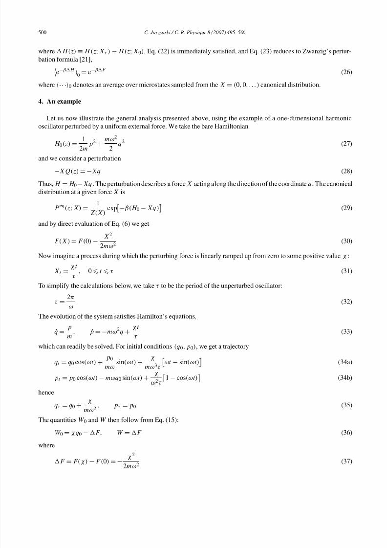
Fig. 1 depicts the distributions ρ0 and ρ. Note that W is negative, while the mean value of W 0 is positive. We can

understand this sign difference as follows. Suppose we adopt the exclusive convention and take the internal energy of

the system to be given by H 0. We imagine that the particle evolves in a fixed harmonic well

U 0(q) = mω2q2/2 (42)

under the influence of a time-dependent external force Xt . The initial position q0 is sampled from a Gaussian distri-

bution centered at q = 0, and as we turn on the perturbing force from 0 to χ , we displace the particle rightward by a

net amount q = qτ − q0 = χ/mω2 (Eq. (35)). The final condition qτ is then distributed as a Gaussian whose mean

no longer coincides with the center of the fixed harmonic well, but rather has shifted by a distance q , as shown inFig. 2. In effect, the perturbation pushes the particle distribution rightward along the q-axis, and ‘up’ the quadratic

potential energy landscape, resulting in a positive value for the average work, W 0 > 0.

Now suppose that we instead choose the inclusive convention and use the full Hamiltonian H = H 0 − Xq to define

the internal energy of the system. Thus we imagine a particle moving in a time-dependent potential,

U t (q) = U 0(q) − Xt q =mω2

2

q −

q

τ t

2

+ F ·t 2

τ 2(43)

Fig. 1. Distributions of work values W 0 and W for the harmonic oscillator example, with χ = m = ω = 1.0 and kB T = 0.3. The distribution ρ is adelta-function at F = −0.5, while ρ0 is a Gaussian whose mean is at −F .




Fig. 2. The bare harmonic potential U 0 is shown, along with the

distributions of initial particle positions (dark gray) and final parti-

cle positions (light gray). As we turn on the force X, we shift the

distribution by an amount q = χ/mω2 = 1.0 away from the min-imum of the potential, resulting in an average increase in the value

of U 0.

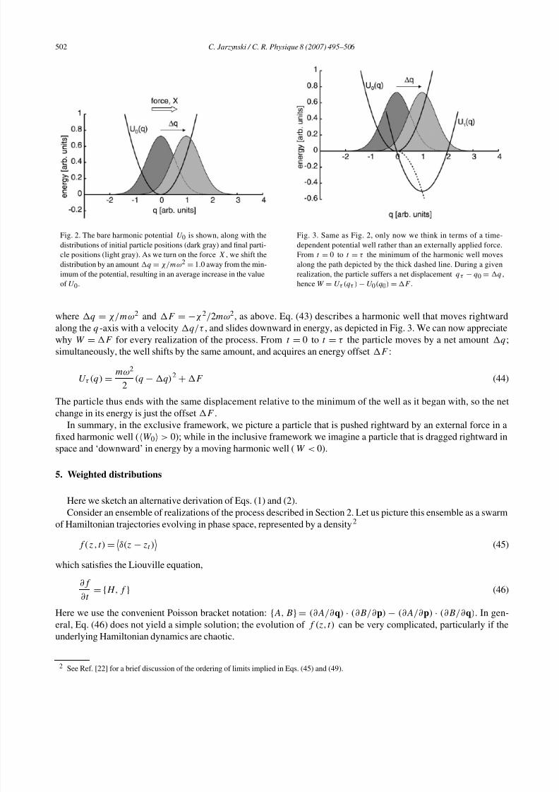
Fig. 3. Same as Fig. 2, only now we think in terms of a time-

dependent potential well rather than an externally applied force.

From t = 0 to t = τ the minimum of the harmonic well moves

along the path depicted by the thick dashed line. During a givenrealization, the particle suffers a net displacement qτ − q0 = q ,

hence W = U τ (qτ ) − U 0(q0) = F .

where q = χ/mω2 and F = −χ 2/2mω2, as above. Eq. (43) describes a harmonic well that moves rightward

along the q-axis with a velocity q/τ , and slides downward in energy, as depicted in Fig. 3. We can now appreciate

why W = F for every realization of the process. From t = 0 to t = τ the particle moves by a net amount q;

simultaneously, the well shifts by the same amount, and acquires an energy offset F :

U τ (q) =mω2

2(q − q)2 + F (44)

The particle thus ends with the same displacement relative to the minimum of the well as it began with, so the net

change in its energy is just the offset F .

In summary, in the exclusive framework, we picture a particle that is pushed rightward by an external force in a

fixed harmonic well (W 0 > 0); while in the inclusive framework we imagine a particle that is dragged rightward in

space and ‘downward’ in energy by a moving harmonic well (W < 0).

5. Weighted distributions

Here we sketch an alternative derivation of Eqs. (1) and (2).

Consider an ensemble of realizations of the process described in Section 2. Let us picture this ensemble as a swarm

of Hamiltonian trajectories evolving in phase space, represented by a density2

f (z,t) =δ(z − zt )

(45)

which satisfies the Liouville equation,

∂f

∂t = {H, f } (46)

Here we use the convenient Poisson bracket notation: {A, B} = (∂A/∂q) · (∂B/∂p) − (∂A/∂p) · (∂B/∂q). In gen-

eral, Eq. (46) does not yield a simple solution; the evolution of f (z,t) can be very complicated, particularly if the

underlying Hamiltonian dynamics are chaotic.

2 See Ref. [22] for a brief discussion of the ordering of limits implied in Eqs. (45) and (49).




For a given trajectory zt , let

w0(t ) =

t 0

dt

k

Xk (t )Qk (zt ) (47)

denote the amount of work performed on the system to time t , using the definition of work corresponding to theexclusive framework (Eq. (10a) and Refs. [13–16]). Since the rate of change of the observable Qk along a trajectory

zt is given by Qk = {Qk , H } [23], we can rewrite Eq. (47) as

w0(t ) =

t 0

dt {X · Q, H } =

t 0

dt {X · Q, H 0} (48)

The last equality follows from the identity {X · Q, X · Q} = 0. Now consider a weighted phase space density

g0(z,t) =δ(z − zt ) exp

−βw0(t)

(49)

in which each trajectory carries a statistical weight, exp[−βw0(t)] (see the discussion below). This density satisfies

∂g0

∂t = {H, g0} − β{X · Q, H 0}g0 (50)

where the second term on the right accounts for the evolving statistical weights. The derivation of this equation is very

similar to those found in Section II of Ref. [3] and Section 4.1 of Ref. [22].

Since w0(0) = 0 identically, and since we assume our ensemble is initially prepared in equilibrium, we have

g0(z, 0) = f(z, 0) = P eq(z; X0). Given these initial conditions, the unique solution of Eq. (50) is the time-independent

distribution

g0(z,t) =1

Z(X0)exp

−βH 0(z)

= P eq(z; X0) (51)

To see this, note thatH, e−βH 0

= −β{H, H 0}e−βH 0 = β{X · Q, H 0}e−βH 0 (52)

using the derivative rule for Poisson brackets, and the identity {H 0, H 0} = 0. From this result it follows by inspection

that Eq. (51) satisfies Eq. (50).

The functions f (z,t) and g0(z,t) are two different statistical representations of the same ensemble of realizations.

Continuing to picture this ensemble as a swarm of trajectories evolving in phase space, f (Eq. (45)) can be viewed

as a number density, which simply counts how many trajectories are found in the vicinity of z at time t ; while g0

(Eq. (49)) can be interpreted as a mass density, if we imagine that each realization carries a fictitious, time-dependent

mass exp[−βw0(t)]. Eq. (51) then has the following interpretation: when the initial conditions are sampled from

equilibrium, the ‘mass density’ of trajectories remains constant in time, even as the ‘number density’ evolves in a

possibly complicated way. Thus while the number of trajectories found near a given point z changes with time, these

fluctuations are balanced by the evolving statistical weights (fictitious masses) of those trajectories, in precisely sucha way as to keep the local mass density constant.

We can obtain analogous results in the inclusive framework (Eq. (10b) and Refs. [2,3]). Introducing

w(t) = −

t 0

dt

k

Xk(t )Qk (zt ) = −

t 0

dt X · Q (53)

along with the corresponding weighted density

g(z,t) =δ(z − zt ) exp

−βw(t)

(54)

we obtain the equation of motion [3,22]

∂g∂t

= {H, g} + βXQg (55)




For initial conditions g(z, 0) = f(z, 0) = P eq(z; X0), the unique solution is

g(z,t) =1

Z(X0)exp

−βH(z; Xt )

=

Z(Xt )

Z(X0)P eq(z; Xt ) (56)

The weighted density is no longer constant in time (as was the case with g0), but rather is proportional to the equilib-

rium distribution corresponding to the current value of the parameters X.The results just obtained are summarized as follows:δ(z − zt ) exp

−βw0(t)

= P eq(z; X0) (57a)

δ(z − zt ) exp

−βw(t)

=Z(Xt )

Z(X0)P eq(z; Xt ) (57b)

Eqs. (1) and (2) now follow immediately by evaluating Eq. (57) at t = τ and integrating both sides over phase space.

While the derivations presented here are less elementary than those of Section 3, we ultimately gain a stronger set of

results. By a simple trick of statistical reweighting, we transform an equation of motion that we cannot solve (Eq. (46))

into one that is easily solved (Eq. (50) or (55)). The result, Eq. (57), allows us to reconstruct equilibrium distributions

P eq using trajectories driven away from equilibrium.

Eqs. (57a) and (57b) are in fact equivalent. Multiplying both sides of Eq. (57a) by exp [+βXt

· Q(z)] and pulling

this factor inside the angular brackets, we obtain Eq (57b). Conversely, multiplication by exp [−βXt · Q(z)] leads us

from Eq. (57b) to Eq. (57a). However, this equivalence is lost once we integrate over phase space: Eqs. (1) and (2) do

not imply one another.

Eq. (57b) can be viewed as a direct consequence of the Feynman–Kac theorem; this observation by Hummer

and Szabo serves as a starting point for their method of reconstructing equilibrium potentials of mean force from

single-molecule manipulation experiments carried out away from equilibrium [7]. Moreover, Eq. (57a) is essentially

a special case of Eq. 12 of Ref. [7] (with W 0 as generalized by Eq. (59) below), if we assume that their confining

potential is initially turned off: u(z, 0) = 0. For an alternative approach to estimating potentials of mean force from

similar experiments, see the ‘clamp-and-release’ method proposed by Adib [24].

6. Discussion

The nonequilibrium work theorem, Eq. (1), has generated interest (and controversy [25–27]) primarily for two

reasons. First, along with the fluctuation theorem for entropy production [28–33], it is one of relatively few equalities

in statistical physics that apply to systems far from thermal equilibrium. Note that the term ‘fluctuation theorem’ has

also been used to specify a relation between the response of a system to external perturbations, and a correlation

function describing fluctuations of the unperturbed system [34,35]. Second, Eq. (1) predicts that equilibrium free

energy differences can be determined from irreversible processes, counter to expectations that irreversible work values

can only place bounds on F [36]. Eq. (2) shares the first feature—it remains valid far from equilibrium—but not the

second; it does not seem to be the case that F can be determined solely from a distribution of values of W 0.

A crucial distinction in this paper has been the difference between the quantities W and W 0. The recognition that,

in the literature, various meanings are assigned to the term work , might at first come as an unwelcome surprise. Work

is a concept of such central importance in thermodynamics that it ought to be unambiguously defined! However, indealing with a physical situation that involves the mechanical perturbation of a system, the perturbation is often ac-

complished by coupling externally controlled variables (X1, X2, . . .) to generalized system coordinates (Q1, Q2, . . .).

This coupling is represented by a term of the form −

k Xk Qk (or a nonlinear generalization thereof, see below) in

the full Hamiltonian that governs the evolution of the system and its surroundings. We are then faced with the question

of whether or not to view this term as part of the internal energy of the system of interest. As stressed in this paper,

either choice is acceptable—this is a question of book-keeping rather than principle—but it is precisely this freedom

that leads to the ambiguity in the definition of work. For related discussions of this issue, particularly in the context of

interpretation of experimental data, see Refs. [37–39,9].

Throughout this paper it has been assumed, following Refs. [13–16], that the coupling between the forces X and the

observables Q is linear: H = H 0 − X · Q. However, as already observed by Bochkov and Kuzovlev, this assumption

can easily be relaxed. Had we written the Hamiltonian as

H (z; X) = H 0(z) − h(Q; X) (58)




and assumed h(Q; X0) = 0, then the entire analysis leading to Eqs. (1) and (2) would have remained valid, provided

the following definitions of work:

W =

τ

0

dt X ·∂H

∂X, W 0 =

τ

0

dt Q ·∂h

∂Q(59)

We recover Eqs. (3) and (11) with a linear perturbation h = X · Q.

The definition of W 0 depends explicitly on the manner in the which the full Hamiltonian is decomposed into a

bare term and a perturbation. Such a decomposition is often natural. For instance, in single-molecule manipulation

experiments we normally take H 0 to be the undisturbed molecule, while a harmonic interaction term −h represents

the perturbation due to an AFM cantilever or optical trap [7]. In this context it is important to keep in mind that

the derivation of Eq. (2) explicitly assumes that the perturbation is initially ‘off’ (e.g. Eq. (7)). If this assumption is

violated, as is often the case in single-molecule experiments [8,10], then Eq. (2) generally does not hold, although

Eq. (1) remains valid.3

While the analysis here has been carried out using Hamiltonian dynamics, the conclusions remain valid under other

frameworks for modeling the evolution of the system. The connection to the stochastic approach taken in Ref. [7] has

already been noted. Moreover, Eqs. 33 and 34 of Ref. [38], derived for inertial Langevin dynamics, are equivalent toEqs. (1) and (2) of the present paper. For non-inertial (overdamped) Langevin dynamics, similar results follow directly

from the Onsager–Machlup expressions for path-space distributions [40,41].

Finally, recall the Crooks fluctuation theorem [5],

ρF (+W )

ρR (−W )= exp

β(W − F )

(60)

where the subscripts refer to two thermodynamic process ( forward and reverse) that are related by time-reversal of the

protocol used to perturb the system. The Bochkov–Kuzovlev papers contain results that are reminiscent of Eq. (60), for

instance Eq. 7 of Ref. [13] and Eq. 2.12 of Ref. [15]. However, while Crooks uses a definition of work corresponding to

W of the present paper, Bochkov and Kuzovlev use W 0, and their results do not involve F . Moreover, in Refs. [13–

16] the derivations seem to assume that the initial conditions are sampled from the same, unperturbed equilibrium

distribution for both the forward and the reverse process (see e.g. Eq. 2.6 of Ref. [15]). Crooks, by contrast, assumesthat the forward and reverse processes are characterized by different initial equilibrium states, both represented by

canonical distributions [42]. It would be useful to clarify more precisely the relationship between these sets of results.

Acknowledgements

It is a pleasure to acknowledge useful conversations and correspondence with Artur Adib, R. Dean Astumian,

Gavin Crooks, Abhishek Dhar, Peter Hänggi, Gerhard Hummer, and Attila Szabo; and financial support provided by

the University of Maryland (start-up research funds).

References

[1] C. Bustamante, J. Liphardt, F. Ritort, Phys. Today 58 (2005) 43.

[2] C. Jarzynski, Phys. Rev. Lett. 78 (1997) 2690.

[3] C. Jarzynski, Phys. Rev. E 56 (1997) 5018.

[4] For pedagogical derivations of Eq. (1) and related results, see for instance Section 7.4.1 of D. Frenkel, B. Smit, Understanding Molecular

Simulation: from Algorithms to Applications, second ed., Academic Press, San Diego, 2002; or

S. Park, K. Schulten, J. Chem. Phys. 120 (2004) 5946; or

G. Hummer, A. Szabo, Acc. Chem. Res. 38 (2005) 504.

[5] G.E. Crooks, Phys. Rev. E 60 (1999) 2721.

[6] G.E. Crooks, Phys. Rev. E 61 (2000) 2361.

[7] G. Hummer, A. Szabo, Proc. Nat. Acad. Sci. 98 (2001) 3658.

[8] J. Liphardt, et al., Science 296 (2002) 1832.

3 In some situations the difference between W 0 and W is relatively small, and one can be used as a substitute for the other in Eq. (1) [10].However, this issue is separate from the validity of Eq. (2), which requires X0 = 0 (Eq. (7)), or more generally h(Q; X0) = 0.




[9] F. Douarche, S. Ciliberto, A. Petrosyan, I. Rabbiosi, Europhys. Lett. 70 (2005) 593.

[10] D. Collin, et al., Nature 437 (2005) 231.

[11] V. Blickle, et al., Phys. Rev. Lett. 96 (2006) 070603.

[12] C.H. Kiang, N. Harris, in preparation.

[13] G.N. Bochkov, Yu.E. Kuzovlev, Zh. Eksp. Teor. Fiz. 72 (1977) 238; Sov. Phys. JETP 45 (1977) 125.

[14] G.N. Bochkov, Yu.E. Kuzovlev, Zh. Eksp. Teor. Fiz. 76 (1979) 1071; Sov. Phys. JETP 49 (1979) 543.

[15] G.N. Bochkov, Yu.E. Kuzovlev, Physica A 106 (1981) 443.[16] G.N. Bochkov, Yu.E. Kuzovlev, Physica A 106 (1981) 480.

[17] D. Halliday, R. Resnick, J. Walker, Fundamentals of Physics, seventh ed., John Wiley and Sons, 2005.

[18] J.W. Gibbs, Elementary Principles in Statistical Mechanics, Scribner’s, New York, 1902, pp. 42–44.

[19] E. Schrödinger’s, Statistical Thermodynamics, Cambridge, 1962. See the paragraphs found between Eqs. (2.13) and (2.14).

[20] G.E. Uhlenbeck, G.W. Ford, Lectures in Statistical Mechanics, Amer. Math. Soc., Providence, 1963, Chapter I, Section 7.

[21] R. Zwanzig, J. Chem. Phys. 22 (1954) 1420.

[22] C. Jarzynski, in: P. Garbaczewski, R. Olkiewicz (Eds.), Lecture Notes in Physics, vol. 597, Springer Verlag, Berlin, 2002.

[23] H. Goldstein, Classical Mechanics, second ed., Addison–Wesley, Reading, MA, 1980, Chapter 9.5.

[24] A.B. Adib, J. Chem. Phys. 124 (2006) 144111.

[25] E.G.D. Cohen, D. Mauzerall, J. Stat. Mech.: Theor. Exp. (2004) P07006.

[26] E.G.D. Cohen, D. Mauzerall, Mol. Phys. 103 (2005) 2923.

[27] J. Sung, cond-mat/0506214v2.

[28] D.J. Evans, E.G.D. Cohen, G.P. Morris, Phys. Rev. Lett. 71 (1993) 2401–2404.

[29] D. Evans, D. Searles, Phys. Rev. E 50 (1994) 1645.

[30] G. Gallavotti, E.G.D. Cohen, Phys. Rev. Lett. 74 (1995) 2694–2697.

[31] J. Kurchan, J. Phys. A 31 (1998) 3719.

[32] J.L. Lebowitz, H. Spohn, J. Stat. Phys. 95 (1999) 333.

[33] See also numerous references in D.J. Evans, D. Searles, Adv. Phys. 51 (2002) 1529.

[34] P. Hänggi, Helv. Phys. Acta 51 (1978) 202.

[35] P. Hänggi, H. Thomas, Phys. Rep. 88 (1982) 207.

[36] W.P. Reinhardt, M.A. Miller, L.M. Amon, Acc. Chem. Res. 34 (2001) 607.

[37] J.M. Schurr, B.S. Fujimoto, J. Phys. Chem. B 107 (2003) 14007.

[38] O. Narayan, A. Dhar, J. Phys. A 37 (2004) 63.

[39] A. Dhar, Phys. Rev. E 71 (2005) 036126.

[40] L. Onsager, S. Machlup, Phys. Rev. 91 (1953) 1505.

[41] R. Dean Astumian, personal correspondence and cond-mat/0608352.

[42] Recently Eq. (60) has been recovered as the limiting case of an analogous microcanonical result, derived within a Hamiltonian formulation;see B. Cleuren, V. Van den Broeck, R. Kawai, Phys. Rev. Lett. 96 (2006) 050601.

Documents

Jarzynski07 Review