Jaya Algorithm + Savings + 2-Opt Heuristic for Multi ... Adaptive Search Methods, Honey Bee Mating Optimization, etc.) have been adapted for solving a large variant of VRP (VRP, Capacitated

International Journal of Applied Engineering Research ISSN 0973-4562 Volume 13, Number 5 (2018) pp. 2242-2250

© Research India Publications. http://www.ripublication.com

2242

Jaya Algorithm + Savings + 2-Opt Heuristic for Multi-Objective

Capacitated Vehicle Routing Problem with Time Constraints &

Heterogeneous Fleet of Vehicles

Prof. R. J. Dhake*

Associate Professor, Industrial & Production Engineering Department, Vishwakarma Institute of Technology, Pune, India.

Dr. N.R. Rajhans

Professor, Production Engineering & Industrial Management Department, College of Engineering, Pune, India.

Nagesh Bhole

S.Y. B. Tech. Computer Engineering Department, Vishwakarma Institute of Technology, Pune, India.

*(Corresponding Author)

Abstract

Vehicle Routing Problem (VRP) plays a vital role in

distribution and logistics. The current work focuses on

optimum routing of a fleet of pick-up vehicles that collect

parts and components from a large number of suppliers (of

consumer durables manufacturer) located in the three

municipal corporations’ viz., Bruhan Mumbai Municipal

Corporation, Navi Mumbai Municipal Corporation & Thane

Municipal Corporation and a collection center. The objective

is to minimize the total distance travelled, which is directly

proportional to the transportation costs and minimizing the

number of pick-up vehicles. Dynamic nature of the problem

restricts use of exact solution algorithms. The solution is

found using Jaya Algorithm (Meta Heuristic Approach - a

population-based new efficient optimization method that

generates a population of solutions to proceed to the global

solution) & Savings Algorithm with 2-opt improvement

heuristic.

Keywords: Vehicle Routing Problem, Meta-heuristics, Jaya

Algorithm

INTRODUCTION

The Vehicle Routing Problem (VRP), a generalized case of

Traveling Salesman Problem (TSP) introduced by Dantzig

and Ramser (Dantzig, 1959) holds a central place in logistics

management (both inbound and outbound logistics) and is one

of the most widely studied problems in combinatorial

optimization. In the initial period solutions generated were

using classical heuristics viz. sweep, strip, nearest neighbor,

minimal spanning tree, savings algorithm, etc. In the past two

decades however, the much of the research shows the use of

meta-heuristics using mainly two search methods: local search

and population search (Cordeau, 2002).

Vehicle routing problems have been the subject of intensive

research for more than 50 years, due to their great scientific

interest as difficult combinatorial optimization problems and

their importance in many application fields, including

transportation, logistics, communications, manufacturing,

military and relief systems, and so on (Vidal, 2013). Vidal T.

et al, 2013 classified the solution methods for VRP into four

categories: constructive heuristics, improvement heuristics,

meta-heuristics, hybrid methods, and parallel and cooperative

meta-heuristics.

The term “meta-heuristic” was first coined by Glover (1986)

to designate a broad class of heuristic methods that continue

the search beyond the first encountered local optimum. A

somewhat crude but telling definition characterizes meta-

heuristics as heuristics guiding other heuristics. According to

Laporte G, et al, 1986, several meta-heuristics have been

proposed for the VRP. These are general solution procedures

that explore the solution space to identify good solutions and

often embed some of the standard route construction and

improvement heuristics. In a major departure from classical

approaches, meta-heuristics allow deteriorating and even

infeasible intermediary solutions in the course of the search

process. The best known meta-heuristics developed for the

VRP typically identify better local optima than earlier

heuristics, but they also tend to be more time consuming

(Laporte, 1999).

The case refers to inbound logistics network of consumer

durable manufacturer. In this 2-echelon (2 stages) network,

pick up operations are done in two stages. The material is first

collected from 28 suppliers (230 components) located in three

municipal corporations viz., BMC, NMMC & TMC in the

Mumbai region through pick-up / mini-door vehicles (light

commercial vehicles) and consolidated at the collection

centre. This is then cross docked in a single Tata 1610/1613

truck (heavy commercial vehicle) and dispatched to the

manufacturer located 250 km away on a daily basis. A private

transport contractor charges the manufacturer at pre-

determined rates mutually decided through negotiations.

LITERATURE SURVEY

A large variety of algorithms (solution methods) are available

to solve VRP. They primarily fall into three categories viz.,

exact solution algorithms, heuristics and meta-heuristics. The

past two decades have found a growing use of meta-heuristic

techniques which are mostly nature-inspired optimization

algorithms. The metaheuristics explore the global optima

without getting stuck in local optima thereby substantially

improving the quality of solutions. Several metaheuristics



2243

(Ant Colony Algorithm, Genetic Algorithm, Tabu Search,

Simulated Annealing, Particle Swarm Optimization, Greedy

Random Adaptive Search Methods, Honey Bee Mating

Optimization, etc.) have been adapted for solving a large

variant of VRP (VRP, Capacitated VRP, VRP with Time

Windows, Heterogeneous VRP, Multi-Deport VRP, etc.)

Jaya Algorithm

Jaya Algorithm proposed by R.V. Rao (R.V. Rao, 2016) is

based on the concept that the solution obtained for a given

problem should move towards the best solution and should

avoid the worst solution. Since, then it has been used in

different applications (Zhang, et al 2016; R.V. Rao, et al

2016). Fig.1 shows the flowchart of the algorithm. The

algorithm always tries to get closer to success (i.e. reaching

the best solution) and tries to avoid failure (i.e. moving away

from the worst solution).

Figure 1: Flowchart of Jaya Algorithm

Jaya Clustering

Clustering procedure using Jaya

Clarke and Wright Savings Heuristic



2244

The Clarke and Wright savings heuristic is the most popular

heuristic, which has withstood the test of time on account of

its speed, simplicity and reasonably good accuracy (Clarke,

1964). The solution quality is improved using 2-Opt method.

1. Problem Description

The firm under consideration is a consumer durable

manufacturer which collects parts and components (more than

560 in variety) from its suppliers (nodes) located in three

municipal corporations’ viz., Bruhan Mumbai Municipal

Corporation, Navi Mumbai Municipal Corporation & Thane

Municipal Corporation. The pickup operations are outsourced

to a third-party transporter and are based on past experience.

The vehicles need to ply through the densely populated areas

and need to adhere to time windows and capacity constraints.

These supplies are then brought to a collection center (depot)

from where these are subsequently shipped to the

manufacturing plant through a heavy commercial vehicle on a

daily basis. In the present practice, four routes are identified

for collecting material from 32 suppliers (nodes) to collection

center (depot) through light commercial vehicles of varying

capacities. The schedule, frequency of collection and other

details of pickup operations, including the transportation costs

is fixed and given in table 1.

The present method of pickup operations highlights the

following problems:

No consideration given to volume and weight of

material transported; vehicle capacities and loading

time required at suppliers. The manufacturer is

charged at a flat rate.

Need for additional trips than scheduled on account

of excess volumes collected from suppliers which are

more than vehicle capacity. This often leads to

additional trips and transportation costs. This

approximately amounts to 20% of the estimated

costs.

The transporter charges the manufacturer at a flat

rate, which leads to excessive transportation costs.

Routes are not optimized considering the volume of

material collected, distance between suppliers,

vehicle capacities.

Need to optimize the pickup operations ensuring FTL

(full truck load), thereby minimizing number of

vehicles required and transportation costs.

PROPOSED METHODOLOGY

Data Collection

The first step is to collect the relevant information related to

the following parameters:

Location of Collection Centre & Suppliers: Distances

in km between suppliers and collection centre

Supplier wise Component Details: Item Code,

Volume per unit.

Daily Requirement for Each Component: As Per

Production Plan.

Supplier wise Collection Volumes: (Based on

Collection Frequency)

Loading Time per Supplier: Total volume collected

per trip and loading time required at each supplier.

Type of Vehicles Available: Number of vehicles of

each type with capacities in volume.

Table-1: Present Practice of Pickup Operations

Route Region

(Location of Suppliers)

Collection Schedule

(Frequency / week)

No. of

Suppliers

Cost Rate Per Trip

(₹ )

Avg. No. of Trips Per

Month

Total Cost Per Route

(₹ )

1 Central Suburban Areas 16 1850 35 64,750

2 Western Suburban Areas 9 1525 32 48,800

3 Greater Mumbai 3 1525 31 47,275

All Routes Annual Transportation Costs (Including Extra Trips ) (₹ ) 1,60,825

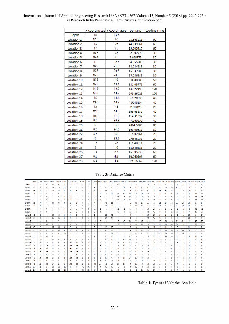
Table 2: Coordinates, Demand (Cubic Feet) and Loading Time(min)



2245

Table 3: Distance Matrix

Table 4: Types of Vehicles Available



2246

Problem Formulation

A fleet of vehicles, based at a single collection centre, collects

a number of consignments from 28 suppliers located in the 3

municipal corporation limits. All orders are consolidated to

full truckloads and are subject to time window constraints.

The underlying assumptions of our model are:

The problem is static; all orders are known a priori.

Transportation cost is directly proportional to the distance

travelled.

Backhauls are not permitted.

All orders are consolidated to full truckloads and don’t

exceed the vehicle capacity.

Time windows for each order have to be adhered strictly.

A tour must not exceed a given time-span. This

assumption models legal restrictions on the maximum

driving time for truck drivers. It could also be viewed as a

restriction, which ensures that maintenance intervals for

vehicles are respected.

Each vehicle has to start and return to the collection

centre after each tour.

Since all components have high volume-weight ratio, the

constraint for their transportation is volume rather than

weight. The requirement of these components remains

fixed over one month period and is specified by

manufacturer through its firm production plan.

Average Vehicle Speed: 20 kmph (Suppliers to

Collection Centre)

Working Hours At Suppliers: Between 8.00 am to 6.20

pm

Fisher and Jaikumar (1978, 1981) developed a three-index

vehicle flow formulation for VRPs with capacity restrictions,

time windows and no stopping times. Such formulations use

variables to represent the passing of a vehicle on an arc or

edge (i, j). In three-index formulations, variables xijk indicate

whether (i, j) is traversed by vehicle k or not. In two-index

formulations, variables xij do not specify which vehicle is used

on (i, j). Define binary variables xijk (i≠j), equal to 1 if and

only if in the optimal solution, arc (i, j) is traversed by vehicle

k. Also define binary variables yik equal to 1 if and only if

vertex i is served by vehicle k. The time windows are two-

sided, meaning that a customer must be serviced at or after its

earliest time and before its latest time. If a vehicle reaches a

customer before the earliest time it results in idle or waiting

time. A vehicle that reaches a customer after the latest time is

tardy. A service time (loading / unloading) is also associated

with servicing each customer. The route cost of a vehicle is

the total of the traveling time (proportional to the distance)

and service time taken to visit a set of customers.

Decision Variables

VRP is a combinatorial problem whose ground set is the edges of a graph G (V, E). The notation used for this problem is as

follows:

G = (V, E): the graph representing the vehicle routing network with vertices V= {v0, v1, v2…, vn} and

E = {(vi, vj)│vi, vj ∈V, i < j} is an arc set

V = {v0, v1, v2…,vn} vertex set where v0 represents depot location and v1, v2…,vn represent customer locations

n = number of nodes corresponding to customer locations for each instance (trip or route)

o = depot location

k = kA + kB, number of pick-up vehicles of type A and B respectively

m = total number of trips corresponding to number of vehicles used

dij = distance (proportional to travel time) between vertices vi and vj (non-negative) (i≠ j)

tij = travel time (proportional to distance) between vertices vi and vj (non-negative) (i≠ j)

ei = earliest arrival time at customer i (i = 1,..,n)

li = latest arrival time at customer i (i = 1,..,n)

ti = total travel time to reach customer i (i = 1,..,n)

si = service time for customer i (i = 1,..,n)

T = maximum travel time permitted for vehicle (T = 620)

Tk = total travel time (including service time) for a vehicle route k (k=1,..,m)

Ei = earliest time allowed for pickup to customer i.

Li = latest time allowed for pickup to customer i.



2247

T = maximum travel time permitted for a vehicle

qi = supply from node corresponding to customer location vi

Q = {

𝑄𝐴 if vehicle is of type A 𝑄𝐵 if vehicle is of type B

(QA: 2050, QB: 5200)

xijk = {

1, if vehicle k travels directly from node 𝑣𝑖 to node v𝑗

0, otherwise

(i, j) = 0,1,..,n) (k = 1,.,m)

yik = {

1, if node 𝑣𝑖 is serviced by vehicle k0, otherwise

(i, = 0,1,..,n) (k = 1,.,m)

Variables xijk and xjik are only defined if qi + qj ≤ Q

Objective Function

𝑀𝑖𝑛 ∑ ∑ 𝑑𝑖𝑗𝑥𝑖𝑗𝑘

𝑛

𝑗=0

𝑛

𝑖=0

(6)

(Minimize total distance travelled (transportation costs)

𝑀𝑖𝑛 𝑚 (7)

(Minimize number of trips corresponding to the number of vehicles

Constraints

∑ 𝑞𝑖𝑦𝑖𝑘 ≤

𝑛

𝑖=0

𝑄𝐴 𝑜𝑟 𝑄𝐵 (𝑘 = 1,2, … . 𝑚) (8)

(Prevent vehicles from carrying loads more than their capacity QA or QB)

∑ 𝑦𝑖𝑘 =

𝑚

𝑘=1

{𝑚, (𝑖 = 0) 1, (𝑖 = 1,2, … , 𝑛)

(9)

(Ensures that each vehicle leaves and arrives at the depot exactly once and each customer is served by one and only one vehicle)

∑ 𝑥𝑖𝑜𝑘 = 𝑚

𝑛

𝑖=0

(10)

(Ensures that the vehicles leave once at each node and m times at the depot o)

∑ 𝑥𝑜𝑗𝑘 = 𝑚

𝑛

𝑗=0

(11)

(Ensures that the vehicles arrive at each node once and leaves the depot o - m times)

m = k (12)

(Ensures that the total number of trips is equal to the total number of vehicles)

∑ ∑ 𝑦𝑖𝑘 (𝑡𝑖𝑗

𝑛

𝑗=0

+ 𝑠𝑖) ≤ 𝑇𝑘

𝑛

𝑖=0

(𝑘 = 1,2, . . , 𝑚) (13)

(Ensures that the vehicles adhere to the time windows)

𝑒𝑖 ≥ 𝐸𝑖 (i, = 0,1,…,n) (14)

(Ensures that arrival time at any customer should not be before earliest time allowed for pickup)



2248

𝐿𝑖 ≥ 𝑙𝑖 (i, = 0,1,…,n) (15)

(Ensures that arrival time at any customer should not be after latest time allowed for pickup)

𝑡𝑗 ≥ 𝑡𝑖 + 𝑡𝑖𝑗 − (1 − 𝑥𝑖𝑗𝑘). 𝑇 (i, j = 0,1,…,n) (k=1,2,..,m) (16)

(Ensures that arrival times between two customers are compatible)

𝑎𝑖 ≤ 𝑡𝑖 < 𝑙𝑖 (i = 0,1,…,n) (17)

(Enforces the arrival time of a vehicle at a customer site to be within the customers earliest and latest arrival times)

𝑡𝑖 ≥ 0 (i = 0,1,…,n) (18)

(Ensures that the arrival time of the vehicle at a customer location is always positive)

Solution Approach based on Jaya Algorithm Based

Clustering (Cluster First and Route Second)

In this method, Jaya algorithm is first applied to form clusters

and subsequently the optimum route is found by Savings

Algorithm.

The principle idea behind Jaya is based on the concept that the

solution obtained for a given problem should move towards

the best solution and should avoid the worst solution.

X&Y coordinates of the centroid of each cluster is considered

as subjects and each student corresponds to a set of pre-

defined centroids. For every student, clusters are generated

using the following logic: Each customer is allocated to the

nearest centroid if it satisfies the time and capacity constraint.

If not, it is allocated to the second nearest centroid, if not to

the third nearest and the process repeats till all allocations are

done. The fitness function is defined as total distance travelled

by each candidate which is nothing but the total route

distance.

Figure 2: Cluster First – Route Second Logic

Steps in Application of Jaya + Savings Algorithm to Vehicle

Routing Problem



2249

1. Define Optimization Problem & Initialize

Optimization Parameters:

Objective Function: Minimize f(x): Minimize total

distance travelled (proportional to transportation

time and costs) and total number of vehicles

Population size Pn: 100 (Number of candidate

solutions)

Design variables Dn: 2

Iterations :50

No. of routes required to serve all customers are

calculated as follows (rounded to next integer):

𝐼𝑛𝑖𝑡𝑖𝑎𝑙 𝑁𝑜. 𝑜𝑓 𝑅𝑜𝑢𝑡𝑒𝑠 (𝑉𝑒ℎ𝑖𝑐𝑙𝑒𝑠) =

𝑇𝑜𝑡𝑎𝑙 𝑑𝑒𝑚𝑎𝑛𝑑 𝑎𝑡 𝑎𝑙𝑙 𝑐𝑢𝑠𝑡𝑜𝑚𝑒𝑟𝑠

𝑉𝑒ℎ𝑖𝑐𝑙𝑒 𝑐𝑎𝑝𝑎𝑐𝑖𝑡𝑦

The number of routes is incremented by 1 in case we

fail to obtain feasible solution.

Lower and upper limits for the centroid values are

(LL, UL): LL ≤ xi ≤ UL

LL = [6.4 1.4 6.4 1.4 6.4 1.4 6.4 1.4]

UL = [18 26 18 26 18 26 18 26]

2. Initialize the Population:

Randomly create the population based on population

size (Pn: 100) and 2 times the number of minimum

routes

3. Identify Initial Solution:(Formation of Clusters &

Route for First Iteration)

Determine best pair of centroids to form the clusters

3.1 Formation of Clusters using the set of centroids

3.1.1 Generate clusters for the set of

centroids given as input

3.1.2 Assign each customer to the nearest

centroid (cluster) such that these satisfy

the constraints viz., vehicle capacity,

time window (travel time + loading

time)

3.1.3 Generate network of clusters formed

3.2 Formation of Route for the given clusters

3.2.1.1 Initialize new route, ordered

matrix and savings matrix

3.2.1.2 Calculate savings matrix and list

the savings in ascending order in

the ordered matrix

3.2.1.3 Calculate all other routes their

distance, time and capacity for the

same

3.2.1.4 Return the formed clusters and

total minimum distance and

maximum distance calculated for

all routes

4. Generate new solution repeating step 3 till all the

iterations are performed (Pn: 100)

4.1 Modify the solution based on best and worst

solutions as

X'j,k,i = Xj,k,i + r1,j,i (Xj,best,i - │Xj,k,i│) - r2,j,i

(Xj,worst,i - │Xj,k,i│)

4.2 Select Best of the previous Two Solutions:

Accept the new solution if it is better than

previous solution, else reject it and retain the

previous solution

The algorithm was run for 20, 50 and 100 population and 2

design variables. However, it was observed that the results

were remaining the same after 12 iterations. On generation of

each cluster, permutations of all possible routes were done to

determine the optimum route within each cluster. The solution

space available for Jaya Algorithm increases substantially.

This gives rise to the possibility of better solutions. Figure 3

shows the number of iterations required to get the optimized

solution.

Figure 3: No. of Iterations vs Solution Quality

Proposed Solution

Determine monthly requirements for each

component (from firm production plan)

Calculate total volume to be collected from each

supplier (for all components)

Determine frequency of optimum pickup runs

for local collection and number of trips required

from Mumbai to manufacture.

Solve the problem as VRP

Figure 4: Formation of Routes & Final Solution

The optimal route formation (including the individual route

distance and time) and the total distance and time travelled is

shown in figure 4.



2250

RESULTS & FINDINGS

The benefits derived from the proposed method in terms of

number of trips, transportation costs and savings is

summarized in table 5 below.

The proposed method of payment to transporter on the basis

of mileage travelled yields substantial savings compared to

the present method of fixed charge per route.

Table 5: Comparison of Existing & Proposed Methods

Existing Method Proposed Method

Total No. of Trips 98 120

Transportation Cost

Calculations

Fixed Charge Per Route

(₹ 18 / km)

Distance Travelled: 193 km (daily), 5790 km

(monthly), 69,480 (yearly)

Total Transportation Cost: ₹ 1,60,825 / month

₹ 19,29,900 / year

₹ 104,220 / month

₹ 12,50,640 / year

Net Savings: ₹ 56,605 per month (₹ 6,79,260 per annum) [35.2 %]

CONCLUSION

The paper addresses a real-life case study for consumer

durable manufacturer of optimization of routes for

collection and transportation of components from

suppliers to collection centre. A new hybrid

metaheuristic based on Jaya Algorithm and Savings

Algorithm is introduced to multi-objective capacitated

vehicle routing problems with time constraints. This

new method is based on cluster first and route second

approach. This technique uses combination of Jaya

heuristic (which explores a large number of cluster

formations and hence enhances the possibility of better

solutions) and Savings Algorithm with 2-Opt

improvement heuristic. Computational results show the

possibility of maintaining solution quality.

REFERENCES

[1] Dantzig, G. B., & Ramser, J. H. (1959). The truck

dispatching problem. Management science, 6(1), 80-

91

[2] Cordeau, J. F., Gendreau, M., Laporte, G., Potvin, J.

Y., & Semet, F. (2002). A guide to vehicle routing

heuristics. Journal of the Operational Research

society, 53(5), 512-522.

[3] Vidal, T., Crainic, T. G., Gendreau, M., & Prins, C.

(2013). Heuristics for multi-attribute vehicle routing

problems: A survey and synthesis. European Journal

of Operational Research, 231(1), 1-21.

[4] Laporte, G., Gendreau, M., Potvin, J.-Y., & Semet,

F. (1999). Meta-heuristics for the vehicle routing

problem. Technical report, Les Cahiers du Gerad, G-

99-21.

[5] Ghiani, G., & Improta, G. (2000). An efficient

transformation of the generalized vehicle routing

problem. European Journal of Operational

Research, 122(1), 11-17..

[6] Liong, C. Y., Ismail, W. R., Omar, K., & Zirour, M.

(2008). Vehicle routing problem: models and

solutions. Journal of Quality Measurement and

Analysis, 4(1), 205-218.

[7] Clarke, G., & Wright, J. W. (1964). Scheduling of

vehicles from a central depot to a number of delivery

points. Operations research, 12(4), 568-581.

[8] Eksioglu, B., Vural, A. V., & Reisman, A. (2009).

The vehicle routing problem: A taxonomic

review. Computers & Industrial Engineering, 57(4),

1472-1483.

[9] Rao, R. (2016). Jaya: A simple and new optimization

algorithm for solving constrained and unconstrained

optimization problems. International Journal of

Industrial Engineering Computations, 7(1), 19-34.

[10] Fisher, M. L., & Jaikumar, R. (1981). A generalized

assignment heuristic for vehicle

routing. Networks, 11(2), 109-124.

[11] Laporte, G. (1992). The vehicle routing problem: An

overview of exact and approximate

algorithms. European journal of operational

research, 59(3), 345-358.

[12] S.R. Thangiah. Vehicle Routing with Time Windows

using Genetic Algorithms, Technical Report SRU-

CpSc-TR-93-23, Computer Science Department,

Slippery Rock University, Slippery Rock, PA. 1993.

[13] Dondo, R., & Cerdá, J. (2007). A cluster-based

optimization approach for the multi-depot

heterogeneous fleet vehicle routing problem with

time windows. European Journal of Operational

Research, 176(3), 1478-1507.

[14] MacQueen, J. (1967, June). Some methods for

classification and analysis of multivariate

observations. In Proceedings of the fifth Berkeley

symposium on mathematical statistics and

probability (Vol. 1, No. 14, pp. 281-297).

[15] Zhang, Y., Yang, X., Cattani, C., Rao, R. V., Wang,

S., & Phillips, P. (2016). Tea category identification

using a novel fractional Fourier entropy and Jaya

algorithm. Entropy, 18(3), 77.

[16] Rao, R. V., More, K. C., Taler, J., & Ocłoń, P.

(2016). Dimensional optimization of a micro-channel

heat sink using Jaya algorithm. Applied Thermal

Engineering, 103, 572-582.

Documents

Jaya Algorithm + Savings + 2-Opt Heuristic for Multi ... Adaptive Search Methods, Honey Bee Mating Optimization, etc.) have been adapted for solving a large variant of VRP (VRP, Capacitated