Differential Geometry

J.B. Cooper

1995

Inhaltsverzeichnis

1 CURVES AND SURFACES—INFORMAL DISCUSSION 2

1.1 Surfaces . . . . . . . . . . . . . . . . . . . . . . . . . . . . . . . . 13

2 CURVES IN THE PLANE 16

3 CURVES IN SPACE 29

4 CONSTRUCTION OF CURVES 35

5 SURFACES IN SPACE 41

6 DIFFERENTIABLE MANIFOLDS 59

6.1 Riemann manifolds . . . . . . . . . . . . . . . . . . . . . . . . . . 69

1

1 CURVES AND SURFACES—INFORMAL

DISCUSSION

We begin with an informal discussion of curves and surfaces, concentrating onmethods of describing them. We shall illustrate these with examples of classicalcurves and surfaces which, we hope, will give more content to the material of thefollowing chapters. In these, we will bring a more rigorous approach.

Curves in R2 are usually specified in one of two ways, the direct or parametricrepresentation and the implicit representation.For example, straight lines have adirect representation as

{tx+ (1− t)y : t ∈ R}

i.e. as the range of the function

φ : t 7→ tx+ (1− t)y

(here x and y are distinct points on the line) and animplicit representation:

{(ξ1, ξ2) : aξ1 + bξ2 + c = 0}

(where a2 + b2 6= 0) as the zero set of the function

f(ξ1, ξ2) = aξ1 + bξ2 − c.

Similarly, the unit circle has a direct representation

{(cos t, sin t) : t ∈ [0, 2π[}

as the range of the function t 7→ (cos t, sin t) and an implicit representation {x :ξ21 + ξ22 = 1} as the set of zeros of the function f(x) = ξ21 + ξ22 − 1.

We see from these examples that the direct representation displays the curveas the image of a suitable function from R (or a subset thereof, usually an in-terval) into two dimensional space, R2. A good model for this is to regard theindependent variable t as time and the curve as the path covered by a movingparticle. The implicit definition specifies the curve as the set {x : f(x) = 0} ofzeros of a function of two variables. These can be conveniently grasped intuitivelyas one of the contours f = c of the surface of the form ξ3 = f(ξ1, ξ2) (figure 1).

Examples of curves with implicit representations arethe ellipse

ξ21a2

+ξ22b2

= 1

2

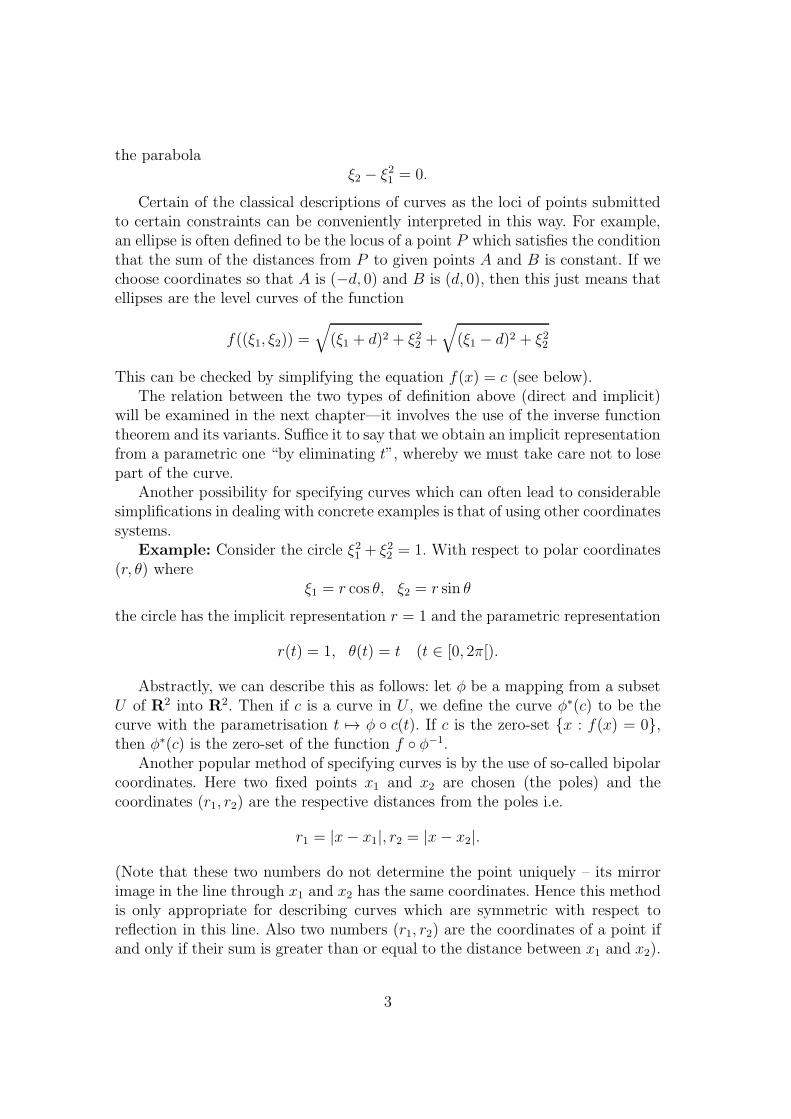
the parabolaξ2 − ξ21 = 0.

Certain of the classical descriptions of curves as the loci of points submittedto certain constraints can be conveniently interpreted in this way. For example,an ellipse is often defined to be the locus of a point P which satisfies the conditionthat the sum of the distances from P to given points A and B is constant. If wechoose coordinates so that A is (−d, 0) and B is (d, 0), then this just means thatellipses are the level curves of the function

f((ξ1, ξ2)) =√

(ξ1 + d)2 + ξ22 +√

(ξ1 − d)2 + ξ22

This can be checked by simplifying the equation f(x) = c (see below).The relation between the two types of definition above (direct and implicit)

will be examined in the next chapter—it involves the use of the inverse functiontheorem and its variants. Suffice it to say that we obtain an implicit representationfrom a parametric one “by eliminating t”, whereby we must take care not to losepart of the curve.

Another possibility for specifying curves which can often lead to considerablesimplifications in dealing with concrete examples is that of using other coordinatessystems.

Example: Consider the circle ξ21 + ξ22 = 1. With respect to polar coordinates(r, θ) where

ξ1 = r cos θ, ξ2 = r sin θ

the circle has the implicit representation r = 1 and the parametric representation

r(t) = 1, θ(t) = t (t ∈ [0, 2π[).

Abstractly, we can describe this as follows: let φ be a mapping from a subsetU of R2 into R2. Then if c is a curve in U , we define the curve φ∗(c) to be thecurve with the parametrisation t 7→ φ ◦ c(t). If c is the zero-set {x : f(x) = 0},then φ∗(c) is the zero-set of the function f ◦ φ−1.

Another popular method of specifying curves is by the use of so-called bipolarcoordinates. Here two fixed points x1 and x2 are chosen (the poles) and thecoordinates (r1, r2) are the respective distances from the poles i.e.

r1 = |x− x1|, r2 = |x− x2|.

(Note that these two numbers do not determine the point uniquely – its mirrorimage in the line through x1 and x2 has the same coordinates. Hence this methodis only appropriate for describing curves which are symmetric with respect toreflection in this line. Also two numbers (r1, r2) are the coordinates of a point ifand only if their sum is greater than or equal to the distance between x1 and x2).

3

For example, if we take the two foci of an ellipse as poles, then the bipolarequation of the latter is

r1 + r2 = 2a.

Similarly, the bipolar equation of a hyperbola, with its foci as poles, is

r1 − r2 = ±2a.

In the above language, we are considering the mapping

φ : x 7→ (|x− x1|, |x− x2|).

Then if c is the line ξ1 + ξ2 = 2d, the ellipse is the pre-image of this curve underφ i.e. the curve φ−1(c).

Many curves are obtained as the images of simple curves (e.g. lines and circles)under suitable analytic or meromorphic functions. For example, straight lines canbe described as follows: let z0 be the (complex number which describes the) pointof reflection of the origin in the line L. Then the vectors z and (z − z0) have thesame length and so there is a complex number ω where ω ∈ T = {ω ∈ C : |ω| = 1}with z − z0 = ωz. This simplifies to the equation

z =z0

1− ω

and so the line is the image of T under the mapping

ω 7→ z01− ω

.

Sometimes it is more convenient to consider the pre-image φ−1(c) of a curve cunder a suitable mapping φ. For example, if c is defined implicitly by the equationf = 0, then its pre-image is the zero-set of the composed function f ◦ φ. Thecommonest examples are obtained by taking the preimages of the coordinate lines(ℜ z = constant,ℑ z = constant) or circles (|z| = constant) under holomorphicmappings φ. Suitable candidates for φ are

z 7→ zn, z 7→ exp z, z 7→ 1

2

(

z +1

z

)

.

For example, the preimages of the axes ξ1 = c resp. ξ2 = d under the mappingz 7→ z2 are the curves

ξ21 − ξ22 = c

resp.2ξ1ξ2 = d.

(Note that these form two mutually orthogonal families of hyperbolas. In fact,families of curves generated in this way – i.e. as the preimages of the coordinate

4

axes under an analytic mapping – are always orthogonal. The reader is invitedto ponder why this is the case).

Another (related) connection between complex numbers and curves is provi-ded by the so-called Schwarz function of a curve. Consider firstly a curve inthe plane given by the implicit equation f(ξ1, ξ2) = 0. If we identify the planeagain with the set of complex numbers C, then we can rewrite this equation inthe form φ(z, z) = 0 for a suitable function φ of two complex variables (in fact,

φ(z, z) = f(z + z

2,z − z

2i)).

Assuming that φ has reasonable properties (we will not concern ourselves herewith the precise details which again involve the implicit function theorem), thenwe can solve the above equation to obtain one of the form z = S(z) whichexpresses z explicitly as a function of z. S is called the Schwarz function of thecurve. For example, the straight line

aξ1 + bξ2 + c = 0

has the Schwarz function

S(z) = −(a− ib)z − 2c

a+ ib

as the reader can verify. Similarly, the Schwarz function of the unit circle isS(w) = 1

w.

Curves and differential equations: It is often helpful to use physical in-terpretations in visualising curves. For example, if we have a curve representedin parametric form x = c(t) then we can regard t as a time variable and c(t) asthe position of the particle at time t so that the curve describes its motion in theplane. More generally, the coordinates of x can represent generalised coordinatesin some phase space, for example, in the mathematical formulation of Newtonianmechanics, the vector x could represent in the first coordinate the position of aparticle moving with one degree of freedom and in the second coordinate velocity.Such curves arise typically as solutions of differential equations of the form

x = f(x, t)

where x = (ξ1(t), ξ2(t)). The above equation is thus equivalent to the system

ξ1 = f1(ξ1, ξ2, t) ξ2 = f2(ξ1, ξ2, t).

Example: Consider a particle with one degree of freedom. If its position isrepresented in some coordinate system by the variable ξ(t), then the general formof Newton’s equation prescribes a second order ordinary differential equation ofthe form

ξ(t) = F (ξ(t), ξ(t), t)

5

for a suitable function F. If we introduce the vector function

x(t) = (ξ1(t), ξ2(t))

where ξ1(t) = ξ(t) and ξ2(t) = ξ(t), then this becomes

x(t) = f(x(t), t)

where f1(x, t) = ξ2 and f2(x, t) = F (ξ1, ξ2, t). The solutions of these equationsare then trajectories in the phase space of the particle.

We illustrate this with three simple examples:I. Free fall: This corresponds to the equation ξ = −g. The corresponding systemis

ξ1 = ξ2 ξ2 = −g.

II. Movement in a gravitational field emanating from a planet:

ξ =−gr0

(ξ + r0)2

i.e.

ξ1 = ξ2 ξ2 =−gr0

(ξ1 + r)2.

III. A weight under the action of a spring: The second order equation isξ = −α2ξ with corresponding system

ξ1 = ξ2, ξ2 = −α2ξ1.

Note that all of these equations can be written in the form

ξ = F (ξ) = −∂U∂ξ

where U = −∫ ξ

ξ0F (t)dt. (In the above cases we have U(ξ) = gξ, −gr0

ξ+r0,

resp. α2ξ2

2). In this case the solutions of the corresponding system

ξ1 = ξ2 ξ2 = F (ξ1)

have the implicit representation E(x) = c where E is the energy function

ξ222

+ U(ξ1)

(traditionally written E = T + U where T is the kinetic energy and U ispotential energy).

6

This leads to the following mathematical formulation: Let G be an open sub-set of the plane. A vector field on G is a mapping f from G into the plane,whereby we tacitly assume some regularity condition on the field, usually at leastcontinuous differentiability. The field then defines a family of curves, the solutionsof the differential equation x = f(x). The typical behaviour of the solutions canbe described as follows: through every point x0 of G there passes exactly one so-lution of this equation and this determines a covering of G by a family of curves.If the vector field is the gradient of a function i.e. if f has the form ( ∂φ

∂ξ1, ∂φ

∂ξ2)

where φ is a scalar field, then the solution curves have the implicit representationφ(x) = c.

Equations of the form x = f(x) i.e. where the right hand side does not dependexplicitly on time are called autonomous. Then if x is a solution, so are thetranslated curves xc where xc(t) = x(t− c).

Examples of autonomous systems:

ξ1 = ξ1, ξ2 = −ξ2ξ1 = −ξ1, ξ2 = −2ξ2ξ1 = ξ1, ξ2 = ξ1 + ξ2ξ1 = ξ1, ξ2 = −ξ2ξ1 = ξ2, ξ2 = −ξ1ξ1 = −ξ1, ξ2 = −ξ1 + ξ2

Using the differential equation x = f(x) we can define a so-called phase-flow

as follows: if x ∈ R2, we define φt(x) to be the value of the solution x(t) of theequation at time t, starting from the initial value x(0) = x. Then we have therelation

φs+t(x) = φs(φt(x)).

Typically the mappings φs are homeomorphisms of space i.e. we can regardthe flow of the differential equation as generating a continuously changing defor-mation of space, the field lines being the trajectories of single points with respectto these deformations.

Example: For the equation ξ = −ξ with corresponding system

ξ1 = ξ2 ξ2 = −ξ1

we have the solution

x = (ξ1 cos t+ ξ2 sin t, ξ2 cos t− ξ1 sin t)

with initial value x(0) = (ξ1, ξ2). Here φt is the linear mapping with matrix[

cos t sin t− sin t cos t

]

(i.e. a rotation).

7

Often (as in the above example) these homeomorphisms φt are rigid i.e. iso-metries of the plane. This leads to the consideration of phase flows of the form

φt = Tu(t) ◦ f(t)

where f and u are smooth functions, the first taking its values in the family ofisometries (i.e. orthogonal two-by-two matrices), the second in the plane. Thenthe trajectories take the form

c(t) = f(t)(x0) + u(t)

for some starting point x0. Important examples of such curves are the cycloidand its variants which we discuss below:

Remark: The differential equation x = f(x) is often written in classicalnotation in the form

Pdx+Qdy = 0

where

f1(ξ1, ξ2) =1

P (ξ1, ξ2), f2(ξ1, ξ2) =

−1

Q(ξ1, ξ2).

We shall simply regard the notation

Pdx+Qdy = 0

as a convenient short-hand for the system x = f(x) where f is as above.Examples: Examples of such equations are

x(y2 − 1)dx− y(x2 − 1)dy = O

(ax+ by)dx+ (a1x+ b1y)dy = 0

(1 + y2)ydx+ (1 + x2)dy = 0

ydx− xdy = 0.

Systems of curves: In fact, curves seldom occur on their own but ratheras members of suitable families. These can arise in various ways, of which thefollowing examples are probably the most important:a) a curve of the form f(x) = 0 is a member of the family f(x) = c of contoursof the landscape formed by the graph of f .b) the solutions of the equation Pdx+ Qdy = 0 typically form a one-parameterfamily of curves which cover some region of the plane.c) orthogonal families: in applications, one often meets two families of curveswhich are mutually orthogonal. Such families can arise as follows: if the onefamily is the solution to the equation Pdx + Qdy = 0, then the second is thesolution of Qdx− Pdy = 0.d) If φ is a suitable map from the plane (or a suitable subset thereof) into the

8

plane, then φ maps families of curves into new ones. Thus we can obtain exoticfamilies by applying suitable mappings to more humdrum systems (such as thelines parallel to the coordinate axes). Typical examples are obtained by usingholomorphic functions (see above).

We conclude these informal remarks about curves with a list of some clas-sical examples, grouped together according to the most convenient method ofdescribing them.

A. Curves as level surfaces: As mentioned above, these often arise as theloci of points moving under some restraint which can be interpreted as a conditionof the form f(x) = c on the coordinates of the point.I. The ellipse: This is often defined as the locus of a point which moves in such away that the sum of its distances from two fixed points is constant (c.f. figure 4).For reasons which will soon become apparent, we now take the two fixed points(the foci of the ellipse) to be (ae, 0) and (−ae, 0), the constant to be 4a2. Theequation then takes on the form

√

(ξ1 + ae)2 + ξ22 +√

(ξ1 − ae)2 + ξ22 = 4a2

which simplifies toξ21a2

+ξ22b2

= 1

where b2 = a2(1− e2).II. The parabola (figure 4): This is the locus of a point whose distances from agiven point F (the focus) and a given line L (the directrix) are equal. If we takeF to be the point (a, 0) and L to be the line ξ1 = −a, we get the equation

(ξ1 − a)2 + ξ22 = (ξ1 + a)2

which simplies to the familiar form ξ22 = 4aξ1.III. Cassini’s ovals (figure 2: These were so named after being used by the astro-nomer Cassini in his investigation of the two body problem (earth-sun system).They are defined as the locus of a point P which moves in such a way that theproduct of its distances from two fixed points (the poles) is constant. If we take(−a, 0) and (a, 0) as the poles, we get the equation

((ξ1 − a)2 + ξ2)2((ξ1 + a)2 + ξ22) = b4

which simplifies to(ξ21 + ξ22 + a2)2 = b4 + 4a2ξ21 .

These are closed, non-self-intersecting curves for a < b. For a = b the curve is afigure of eight (the Leminiscate of Bernoulli) and for a ≥ b it splits up into twoloops.IV. The Lame curves: This is the family of curves with implicit equations

(ξ21a2

)n

+(ξ22b2

)n

= 1.

9

(For each value of n between zero and infinity we get a separate curve.) Of course,the case n = 1 is the ellipse. The case where n = 1

3is an interesting curve called

the asteroid which we shall discuss later. The case n > 2 gives elegant ovalshapes which are popular in art and design.

B. Curves defined by parametrisations resp. by movements in the

plane:

I. The cycloid (figure 4): This is the path traced by a point on the cicumference ofa circle which is rolled along a line. From figure 3 we see that the vector OP is thesum of the vectors OM and MP i.e. it is (t, 1)−D−t(0, 1) or (t− sin t, 1− cos t).

More generally, if we trace the path of the point with original coordinates x(i.e. not necessarily the path of the origin as above), then we merely replace thevector MP by D−t(x− (0, 1)). This leads to the equation

c(t) = (t+ ξ1 cos t+ (ξ2 − 1) sin t, 1− ξ1 sin t + (ξ2 − 1) cos t).

II. Epicycloids resp. hypocycloids. These are obtained as above but by rolling asmaller circle (of radius r) around a larger one (with radius R). We suppose thatR = nr, whereby n need not be an integer. If the smaller circle is rolled aroundthe exterior of the larger one, we get an epicycloid, otherwise a hypocycloid. Themethod used above leads to the equations

c(t) = ((n + 1)r cos t− r cos (n+ 1)t, (n+ 1)r sin t− r sin (n+ 1)t)

for the epicycloid and

c(t) = r((n− 1) cos t+ cos(n− 1)t, (n− 1) sinnt− sin(n− 1)t)

for the hypocycloid.Two special cases are of particular interest:

III. The nephroid (figure 4): This is the epicycloid for the case where n = 2. Ithas parametrisation

c(t) = r(3 cos t− cos 3t, 3 sin t− sin 3t).

IV. The cardioid (figure 5): This is the epicycloid with n = 1. It has parametri-sation

c(t) = r(2 cos t− cos 2t, 2 sin t− sin 2t).

C. Curves defined by differential equations:

Recall the general equation x = f(x). The most interesting things happen aroundzeros of the field f (these correspond to states of equilibrium of physical systems).For convenience, we shall assume that this takes place at x = 0 i.e. the equationhas the form x = f(x) where f(0) = 0. Now if we assume that f is smooth, wecan consider its Taylor development. This begins with the linear term (Df)0(x).

10

Hence, neglecting the terms of higher order, we obtain, as an approximation tothe original equation, one with a linear field f on the right hand side i.e. asystem of the form x = Ax where A is a two by two matrix (the Jacobi matrix off at zero). It is plausible (and with the usual suitable restrictions even true) thatthe solution to this linear equation will provide – at least in a neighbourhood ofthe origin – a good approximation to the solution of the general equation. Forthis reason, we shall confine our attention here to such linear systems. For suchequations, one can give a complete description of the solutions. For reasons whichwill be explained shortly, we begin by considering the following four cases:a)

A =

[

λ1 00 λ2

]

where λ1 and λ2 are distinct reals.b)

A =

[

λ1 10 λ1

]

.

c)

A =

[

λ 00 λ

]

for λ real.d)

A =

[

α β−β α

]

where α and β are real.The corresponding solutions area) ξ1 = c1e

λ1t, ξ2 = c2eλ2t.

b) ξ1 = (c1 + tc2)eλt, ξ2 = c1e

λt.c) as a) with equal lambdas.d) r(t) = r0e

αt, θ(t) = βt+ θ0.See figure 7.

In order to justify the choice of the above four types of matrices, we recall someelementary facts from linear algebra. Since our reasoning is completely general,we might just as well deal with the n-dimensional case i.e. with equations of theform x = Ax where A is an n by n matrix and x is a function with values in Rn.Consider firstly the situation where A is diagonalisable i.e. there is an invertiblematrix P so that PAP−1 = D where

D = diag (λ1, ..., λn).

Then the equation can be written in the form P x = DPx i.e. y = Dy wherey = Px. Of course, this has solution

y(t) = (eλ1tη1, . . . , eλntηn)

11

with y(0) = (η1, ..., ηn).The solution of the original equation is then x = P−1y.

Similar techniques can be used when the matrix is not diagonalisable - thenone must use the Jordan or the rational canonical form to reduce to simpler cases.For us it suffices to remark that a linear change of variables can always be foundwhich reduces to the case where A has a suitable simple form. In the case of twoby two matrices, only the four types considered above can occur. They correspondto the situations where A has two distinct real eigenvalues, two coincident realeigenvalues or a pair of complex-conjugate eigenvalues.

D. Curves defined by holomorphic functions:

Here we return to the topic of epi- and hypocycloids. If we refer to figure 6, wesee that the complex number z corresponding to the vector OP has the form

z = OQ+QP = r(n− 1)eiθ + re−iθ(n−1).

Hence if we write w for the complex number eiθ, we see that the hypocycloid isthe image of the unit circle T under the holomorphic mapping z = φ(w) where

φ(w) = r((n− 1)w + w1−n).

It is interesting to note that our general condition on the mapping φ in order tobe able to compose it with curves without introducing a singularity (i.e. that itbe locally a diffeomorphism) fails when φ′(w) = 0. In our case

φ′(w) =r(n− 1)(wn − 1)

wn

and in general there are cusps at the points where this expression vanishes. Forexample, in the case where n = 2 (where the transforming function is z = r(w+1w)) we have two cusps (in fact, this curve is a part of a straight line - a fact which

is used in engineering). For n = 3 we have three cusps. The equation of this curveis

z = r(2w +1

w2).

(The curve is called a deltoid.)In a similar manner, one can calculate that the equation of the epicycloid is

z = r((n+ 1)w + wn+1).

For n = 1, r = 1 we get z = 2w − w2 which is the equation of the cardioid.

E. Curves defined by Schwarz functions:

I. The straight line through z1, z2 has Schwarz function:

S(z) =z1 − z2z1 − z2

z +z1z2 − z2z1z1 − z2

.

12

II. The circle with centre z0 and radius r. The Schwarz function is

S(z) =r2

z − z0+ z0.

III. The ellipse x2

a2+ y2

b2= 1 :

S(z) =a2 + b2

a2 − b2z2 +

2ab

b2 − a2

√z2 + b2 − a2.

F. Curves in polar coordinates:

I. The Rhodoneae: This is the family of curves with polar equations

r = a cos kθresp. r = a sin kθ

where k is a parameter (not necessarily an integer). For integral values, they arerose-like curves. For example, the case k = 4 is a four petalled flower-shape—known as the quadrifolium.

II. The spirals: “Spiralıs a generic name for curves of the form r = f(θ) where fis usually (but not always) positive and monotone. The best known examples are1) the spiral of Archimedes with equation r = aθ;2) the spiral of Fermat with equation r2 = a2θ;3) the spiral or Lituus with equation r2 = a2

θ;

4) the hyperbolic spiral with equation r = aθ;

5) the equiangular spiral with equation r = aθ;6) the sinuisoidal with equation rn = an cosnθ (n a parameter).(See figue 8).

1.1 Surfaces

We now discuss briefly surfaces, more precisely, two dimensional surfaces in three-space. Once again, there are several ways of describing them and we shall con-centrate on the following two:The implicit definition: surfaces are the zero-sets of smooth functions definedon suitable subsets of R3. For example, the sphere is the zero-set of the function

f(x) = ξ21 + ξ22 + ξ23 − 1.

As in the case of curves, such surfaces can be regarded as the level surfaces of ascalar field in space. For example if the scalar field represents a potential, thenthese are the equipotentials. A consideration of concrete examples will speedilypersuade the reader that singularities occur only when the gradient of the scalarfunction f vanishes. (Think of the vertex of the cone ξ23 = ξ21 + ξ22 .)

The parametric definition: Surfaces are the images of (open subsets of)R2 under smooth mappings from the plane into space. For example the mapping

φ : (u, v) 7→ (u, v,√1− u2 − v2)

13

which is defined for u2 + v2 < 1 describes a hemisphere.Once again, simple examples suggest that singularities can only occur when

the rank of the derivative Dφ of φ is not maximal i.e. is either 0 or 1. Geometri-cally, this means that the two vectors D1φ and D2φ (the partial derivatives of φ)are proportional.

Examples of surfaces:

I. Landscapes: These are surfaces of the form ξ3 = f(ξ1, ξ2) i.e. the graph of asmooth function defined on the plane. Such surfaces have the implicit represen-tation F = 0 where F is the function

x 7→ ξ3 − f(ξ1, ξ3)

and the parametric representation

φ(u, v) = (u, v, f(u, v)).

II. Surfaces of revolution (figure 12): these are surfaces obtained by rotating acurve

c(u) = (0, h(u), k(u))

in the (y, z)-plane around the z-axis. They are parametrised by the function

φ : (u, v) 7→ (h(u) cos v, h(u) sin v, k(u)).

If the curve has the implicit form F (ξ2, ξ3) = 0, then the implicit equation of thesurface is

F ((ξ21 + ξ22)1

2 , ξ3) = 0.

A simple and important example of a surface of revolution is the standard conewhich is obtained by rotating the diagonal in the (y, z)-plane about the z-axis.It has thus the implicit representation ξ23 = ξ21 + ξ22 and the parametrisationφ(u, v) = (u cos v, u sin v, u).III. The sphere (figure 9): this has implicit equation

ξ21 + ξ22 + ξ23 = 1.

and parametrisation

φ(u, v) = (cosu cos v, cosu sin v, sinu)

as surface of revolution generated by the unit circle in the (y, z)-plane. (para-metrisations of the sphere are of particular interest since they form the basis ofcartography).IV. The torus: this is also a surface of revolution, this time of a circle as in thediagram.The torus has parametrisation

φ(u, v) = ((a+ b cosu) cos v, (a+ b cosu) sin v, b sin u)

14

where a > b > 0, a and b being the radii of the circles indicated in the diagram.The implicit equation is

(

√

ξ21 + ξ22 − a

)2

+ ξ23 = b2.

V. The cone (figure 10): this is again a surface of revolution, with parametrisation

φ(u, v) = (u cos v, u sin v, u)

and implicit equation ξ23 = ξ21 + ξ22 .Note that at the points u = ±π

2resp. u = v = 0, the parametrisations of the

sphere and the cone are not regular. In the second case, but not in the first, thiscorresponds to a real singularity of the underlying figure.VI. The helicoid (figure 11), with parametrisation

φ(u, v) = (u cos v, u sin v, v) (u, v ∈ R).

VII. The Mobius strip has parametrisation

φ(u, v) = (cosu+ sin u cosu, sin u+ v sin u sin v, v cos u).

VII. Cylinders: these have equations f(x) = 0 where the function has the formf(ξ1, ξ2, ξ3) = g(ξ1, ξ2) for a function g of two variables (i.e. f is independent ofthe third variable). This surface is the cylinder over the plane curve formed bythe zero-set of g.

If φ is the parametrisation of a surface, then the curves

u→ φ(u, v0) v → φ(u0, v)

obtained by holding v resp. u fixed are called the (curvilinear) coordinate lineson the surface (they are just the images of the Cartesian coordinate lines underthe parametrisations). For example, for the parametrisation of the sphere givenabove, they are the familiar lines of latitude and longitude. At a given point onthe surface, the two tangents to these lines span the tangential plane there.More precisely, if φ1 and φ2 denote the partial derivatives of φ and we introducethe mapping

N(u, v) =φ1(u, v)× φ2(u, v)

|φ1(u, v)× φ2(u, v)|(which is called theGaußian mapping), thenN is the unit normal to the surfaceat φ(u, v) and the tangential plane there has he equation

(x− φ(u, v)|N(u, v)) = 0.

The behaviour of N and its derivative provide information on the geometry ofthe surface in a neighbourhood of the given point. This topic will be discussed inmore detail later.

15

2 CURVES IN THE PLANE

In this chapter we shall bring a more systematic and general theory of curves. Theemphasis will be on structural properties rather than on the special character ofparticular curves. We begin with the formal definition of parametrised curves inthe plane:

Definition: A parametrised Cr-curve in R2 is an r-times continuously differen-tiable function c from an interval I in R into R2. The parametrisation is regularif c(t) 6= 0 for all t.

Of course, such a parametrisation contains more information than one usuallyassociates with a geometric curve (if one thinks of a curve as the path of a movingparticle, then the parametrisation also tells us the speed of the particle at agiven moment). Hence we introduce the following concept of equivalence betweenparametrisations. Two parametrisations c1 and c2 are equivalent if there is aCr-bijection φ : I1 → I2 (where the I ′s are the respective domains of definition)such that φ(t) > 0 for each t ∈ I1 and c2 = c1 ◦ φ−1. Such a function φ is calleda reparametrisation. Note that the condition on φ ensures that its inverse isalso Cr. The positivity condition on the derivative means that we are prohibitingreversals of direction.

Of course it would be horribly tedious to distinguish between parametrisati-ons, equivalence classes thereof and the various degrees of regularity. Hence weshall often simply employ the word “curveand leave it to the common sense of thereader to deduce from the context in which precise sense it is being used. If thereis any danger of confusion we shall be more precise in our use of terminology.

The simplest version of the implicit function theorem implies the following: ifc : I → R2 is a regular Cr-curve (for r ≥ 1) and t0 is in the interior of I, thenthere is a neighbourhood V of c(t0) in R2 and a diffeomorphism ψ from V ontoa neighbourhood U of zero in R2 so that ψ ◦ c is equal to the curve t 7→ (t, 0).Note that this implies that locally the curve c is the zero set of a smooth function(namely the second component ψ2 of ψ).

Particularly simple are curves of the form c(t) = (t, f(t)) i.e. the graphs offunctions. In fact all regular curves are locally of this form (again a consequenceof the implicit function theorem). More precisely, choose t0 ∈ I. Since c(t0) 6= 0,either c1(t) 6= 0 or c2(t) 6= 0. Suppose that the former holds. Then there is aneighbourhood U of t0 in I so that c1 is invertible on U . Let φ be an inverse tothe restriction of c1 to U . Then under the reparametrisation φ, the curve has theform u → (u, c2(φ(u)) on U .

Arc-length: If c : [a, b] → R2 is a curve, its length is defined to be

L =

∫ b

a

|c(t)| dt.

16

Geometrically, the length is defined as follows: we choose a partition (t0, t1, . . . , tn)of [a, b] and consider the broken line constructed by joining successively the points(c(t0), c(t1), . . . , c(tn)). The length of the curve is the limit of the lengths of theselines as the partition becomes finer. Since we shall not require this result, we willnot bother to prove it. This can be done easily by writing out explicitly the lengthof the chain and noting that an application of the mean value theorem displaysit as a Riemann sum for the above integral.

We can use the notion of arc length to introduce a natural parametrisationfor curves. If we regard a curve as the path of a moving particle, then there is oneform of motion which obviously enjoys a privileged position among all equivalentones – that for which the speed is uniform. This means that the particle arrivesat a point in a time which is proportional to its distance (along the curve) fromits starting point. Hence we use the reparametrisation φ where

φ(t) =

∫ t

a

|c(u)| du.

It is customary to write s for φ(t). The new parametrisation c ◦ φ−1 is called theparametrisation by arc-length and is traditionally denoted by γ. Thus wehave the relationship

γ(s) = c(t) (s = φ(t)).

When we use the letter γ to denote the parametrisation of a curve in future, thenwe are tacitly assuming that it is parametrised by arc-length. Another generallyemployed convention is to use dashes to denote the derivative with respect to sand Newtonian dots for differentiation with respect to t (thus γ′(s) but c(t)).

If we differentiate the expression γ(s) = c(t) and use the chain rule (recallingthat φ(t) = |c(t)|), then we see that

γ′(s) =c(t)

|c(t)|

(i.e. the derivative of γ is the normalised version of the derivative of c).Now the difference quotients

γ(s+ h)− γ(s)

h

which define the derivative of γ at the point s represent the chord from γs toγ(s + h), almost normalised (since the length of the chord is approximately hwhen h is small). Hence the unit vector γ′(s) is the unit tangent vector to thecurve at s. We denote it by Tγ(s) or, if there is no danger of confusion, simply byT(s). In terms of a general parametrisation c (i.e. not necessarily parametrisationby arc-length), we define

Tc(t) =c(t)

|c(t)| .

17

We now wish to define the curvature of a curve at a point s. Intuitively, itis related to the rate of change of the tangent vector T. We define it to be thereciprocal 1

Rof the radius of that circle which approximates the curve best at the

given point. More precisely, we shall show that under suitable circumstances, ifs1, s2, s3 are near s, then γ(s1), γ(s2), γ(s3) are not collinear and so there is a circlewith centre C(s1, s2, s3) through them. Furthermore, we shall show that as thethree points tend to s, then the centres C(s1, s2, s3) tend to a point. We then definethe circle through γ(s), with centre at this limit, to be the osculating circle ofthe curve at the given point. Its centre (resp. radius) are called the centre of

curvature resp. radius of curvature at s. The inverse of the radius is calledthe curvature at s. The mathematics behind these definitions is contained inthe following Proposition:

Proposition 2.1 Let γ be a C2-curve and suppose that a point s is such thatγ′′(s) 6= 0. Then there is a neighbourhood U of s so that γ(s1), γ(s2), γ(s3) arenot collinear if s1, s2, s3 are distinct points in U . As s1, s2, s3 tend to s, the circlethrough γ(s1), γ(s2), γ(s3) converges to a circle through γ(s) with radius |γ′′(s)|−1

which is tangential to the curve at γ(s).

Proof. Denote the centre of this circle by C(s1, s2, s3) as in the text above andconsider the function

f : s 7→ |γ(s)− C(s1, s2, s3)|2 = (γ(s)− C(s1, s2, s3)|γ(s)− C(s1, s2, s3)).

Thenf ′(s) = 2(γ′(s)|γ(s)− C(s1, s2, s3))

andf ′′(s) = 2

(

γ′′(s)|γ(s)− C(s1, s2, s3))

+ 2.

By the mean value theorem, there are points ξ1, ξ2, ξ3 near s so that f ′(ξ1) =f ′(ξ2) = 0 and f ′′(ξ3) = 0 i.e.

(γ′(ξi)|γ(ξi)− C(s1, s2, s3)) = 0

for i = 1, 2 and(γ′′(ξ3)|γ(ξ3)− C(s1, s2, s3)) = −1

(we are assuming, for convenience, that s1 < s2 < s3).If C(s1, s2, s3) has a limit C when the three points tend to s, we get (γ′(s)|γ(s)−

C) = 0 (or (T(s)|γ(s)−C) = 0). This means that the limiting circle is tangentialto the curve. Furthermore we have

(γ′′(s)|γ(s)− C) = −1.

18

Now if γ′′(s) is not a multiple of γ′(s), then these equations determine C. In fact,γ′(s) is perpendicular to γ′′(s) and both are non-zero by hypothesis. Hence theequations

(γ′(s)|γ(s)− C) = 0

and(γ′′(s)|γ(s)− C) = −1

determine C uniquely. In fact, γ(s)− C = aγ′′(s) where a = −1|γ′′(s)|2

and

|γ(s)− C| = |a||γ′′(s)| = 1

|γ′′(s)| .

We now prove the statement concerning the non-collinearity of γ(s1), γ(s2) andγ(s3). The rest of the result follows then form the calculations above. Suppose the-re are distinct points s1, s2 and s3 which are arbitrarily close to s with γ(s1), γ(s2)and γ(s3) collinear. Then by the mean value theorem, there are points ξ4, ξ5 withξ4 between s1 and s2 and ξ5 between s2 and s3, so that T(ξ4) and T(ξ5) are paral-lel to this line and hence to each other. Then T(ξ4) = ±T(ξ5). By continuity, wemust have T(ξ4) = T(ξ5) if we are near enough to s. This implies the existenceof a ξ6 between ξ4 and ξ5 with T′(ξ6) = γ′′(ξ6) parallel to T(ξ4) = γ′(ξ4). In thelimit, this implies that γ′′(s) is parallel to γ′(s). But γ′′(s) ⊥ γ′(s) and γ′′(s) 6= 0which is a contradition.

In order to show that the centres C(s1, s2, s3) converge, we note that theequations

(γ′(ξ1)|γ(ξ1)− C(s1, s2, s3)) = 0

and(γ′′(ξ3)|γ(ξ3)− C(s1, s2, s3)) = −1

can be written in the matrix form

A(ξ1, ξ3)C(s1, s2, s3) =

[

(γ′(ξ1)|γ(ξ1))1 + (γ′′(ξ3)|γ(ξ3))

]

where

A(s, t) =

[

γ′1(s) γ′2(s)γ′′1 (t) γ′′2 (t)

]

If we let the point converge to s, then we see that since A(ξ1, ξ3) converges to

[

γ′1(s) γ′2(s)γ′′1 (s) γ′′2 (s)

]

and the right hand side converges to

[

(γ′(s)|γ′′(s))1 + (γ′′(s)|γ(s))

]

19

then C(s1, s2, s3) converges to

A(s, s)−1

[

(γ′(s)|γ(s))1 + (γ′′(s)|γ(s))

]

.

The unit normal Nγ(s) (or simply N(s)) to the curve at s is the imageDπ

2Tγ(s) of the tangent vector under the operator of rotation through 90 degrees

(i.e. the mapping (ξ1, ξ2) → (−ξ2, ξ1)). Thus (T(s),N(s)) forms a right handedorthogonal system for the plane.

From the above calculations we know that γ′′(s) is perpendicular to T(s) andso is some multiple of N(s). We can thus define the curvature κ(s) of the curveat s by means of the equation

γ′′(s) = κ(s)N(s).

In other words, the absolute value of the curvature is just the length of the vectorγ′′(s). This means that the curvature is, up to sign, the reciprocal of the radiusof curvature. The sign of κ has the following geometrical significance:

κ > 0 means that the curve is curving towards N;κ < 0 means that the curve is curving away from N.(in both cases in the direction of increasing s.)

We have the following formula for the curvature function:

κ(s) = det

[

γ′1(s) γ′′1 (s)γ′2(s) γ′′2 (s)

]

.

(The above determinant is precisely the signed area of the rectangle spanned bythe vectors γ′(s) and γ′′(s). For this latter expression is

−(γ′(s)|Dπ2γ′′(s)) = −(Tγ(s)| − κ(s)Tγ(s)) = κ(s).)

The above information can be conveniently expressed in the equations:

T′(s) = κ(s)N(s) N′(s) = −κ(s)T(s)

which are known as the Frenet formulae.(In matrix form

[

T′1 T′

2

N′1 N′

2

]

=

[

0 κ−κ 0

] [

T1 T2

N1 N2

]

.

Proof. The first equation is the definition of the curvature function. For thesecond one, we simply differentiate the equation N = Dπ

2T to get

N′ = Dπ2T′ = Dπ

2κN = κDπ

2Dπ

2T = −κT.

20

In order to be able to calculate with general curves (which are not usuallypresented in the convenient form of being parametrised by arc length), we con-strue these formulae in terms of the parametrisation c = γ ◦ φ. Firstly, we definethe curvature and normal to c in the natural way i.e.

κc(t) = κγ(s), Nc(t) = Nγ(s).

Then, by the chain rule,c(t) = γ′(s)φ(t)

c(t) = γ′′(s)φ(t)2 + γ′(s)φ(t).

Using the fact that the curvature is the determinant of the matrix with the vectorsγ′(s) and γ′′(s) as columns, we obtain the formula

κc(t) =c1(t)c2(t)− c1(t)c2(t)

(c1(t)2 + c2(t)2)3

2

.

AlsoTc(t) = Tγ′(φ(t))φ = Tγ′(s)|c(t)| = κγ(s)Nγ(s)|c(t)|

= κc(t)Nc(t)|c(t)|and so the Frenet formulae take on the form:

T = |c|κN N = −|c|κT.

A rather simple calculation shows that, as one would expect, the only curveswith identically zero curvature (resp. with constant, but non-zero curvature) arestraight lines (resp. circles). However, rather than actually carry this out, we shallprove a more general result, namely that the curvature determines the curve upto its position in the plane (i.e. two curves with the same curvature functions arecongruent). On the other hand, as we shall show, any continuous function can bethe curvature function of a curve.

Proposition 2.2 Let f be a continuous, real-valued function on the interval[0, L]. Then there is a curve γ defined on this interval which has f as its curvaturefunction. If γ is a second curve which also has f as its curvature function, thenthe curves γ and γ are congruent.

Proof. Consider the differential equations

T′1 = −f(s)T2, T′

2(s) = f(s)T1.

By a standard existence theorem for linear differential equations, there is a solu-tion T of the above equations which satisfies any suitable initial conditions. We

21

choose any such conditions, whereby |T(0)| = 1. Then the length of the vector isalways one since

(T21 +T2

2)′ = 2(T1T

′1 +T2T

′2) = −f(s)T1T2 + f(s)T1T2 = 0

and so the length of T is constant.If we now take γ to be a primitive of T, then by its very definition this is

a curve, parametrised by arc-length, which satisfies the Frenet formulae, with κreplaced by f . Hence f is the curvature function of γ.

Now if γ is a second such curve, then T = γ′ is also a solution of the abovedifferential equation (but with different inital values). If we choose a rotation Dθ

about zero which maps T(0) onto T(0), then Dθ ◦T is also a solution, this timewith the same initial values as T. Hence, by uniqueness, T coincides with Dθ ◦T.This implies the final statement of the theorem.

A disadvantage of the above definition of curvature is that it only applies tocurves γ for which γ′′ never vanishes. In particular, the curvature of a straightline is not defined. It should, of course, be zero. This can be rectified as follows.We say that a curve γ has a moving frame if there are continuous functionsT,N from [0, L] into the plane and a continuous real-valued function κ on [0, L]so that the pair (T(s),N(s)) forms a right-handed orthonormal basis for each sand the Frenet formulae

T′(s) = κ(s)N(s), N′(s) = −κ(s)T(s)

hold. Also γ′(s) = T(s). κ is then called the curvature function of the curve.Under this definition, straight lines do have zero curvature.

It is clear that the angle between the tangent of a curve and the x-axis variescontinuously along the curve. In order to state this precisely, we require thefollowing Lemma:

Lemma 2.3 Let f be a continuous function from an interval into the circle S1.Then there is a continuous function f from the interval into the real line so thatp◦ f = f where p is the mapping t 7→ (cos t, sin t) from R onto S1. If g is a secondfunction with this property, then the difference f − g is a constant function of theform 2πk for some k ∈ Z.

Proof. For convenience, we suppose that the interval of definition is the unitinterval [0, 1]. By continuity, we can choose an n ∈ N so large that the range off on each interval of the form [ k

n, k+1

n] lies in a half-circle of S1. Choose f(0) to

be some point in R with p(f(0)) = f(0). Now it is clear from the diagram howwe should (even must) define f on [0, 1

n]. We then repeat this process to define f

successively on the intervals [ kn, k+1

n].

22

If g is a second such function, then the difference f−g is a continuous functionwhich takes its values in the set {2πk : k ∈ Z}. But any interval in R is connectedand hence so is its image in the latter set. The only connected subsets of discretespaces are one-point sets and this implies that the difference is constant.

The following generalisation of this result can be proved similarly:

Proposition 2.4 Let G be a subset of the plane which is starlike with respectto a point x0. Then if f is a continuous mapping from G into S1, there is acontinuous lifting f of f i.e. a function from G into R so that p ◦ f = f .

If we apply the above result to the tangent function T of a curve γ, then itguarantees the existence of a continuous function θ so that

T(s) = (cos θ(s), sin θ(s))

(i.e. θ describes in a continuous way the angle between the tangent and the x-axis).

It follows from the above equation that

γ′′(s) = (−θ′(s) sin θ(s), θ′(s) cos θ(s))

and so

Definition 2.5 A first order differential form (or simply a one form) onan open subset U of R2 is a mapping

ω : U ×R2 → R

which is linear in the second variable and smooth in the first one. In other words,it assigns to each point x of U an element of the dual of R2. The standard exampleis the differential df of a smooth function f : U → R where

df(x) : y = (η1, η2) 7→ D1f(x)η1 +D2f(x)η2

(i.e. df(x) is the vector (D1f,D2f)x regarded as an element of the dual of R2 inthe usual way).

In order to develop a more suggestive notation for differential forms, we write ξ1resp. ξ2 for the functions

x 7→ ξ1 x 7→ ξ2

onR2. Then the differentials dξ1 and dξ2 are constant. In fact, the pair (dξ1, dξ2) isjust the canonical basis for the plane and the above formula takes on the familiarform

df = D1fdξ1 +D2fdξ2

23

(df = ∂f

∂xdx+ ∂f

∂ydy in classical notation). If the field f is interpreted as a poten-

tial function, then the above one-form corresponds to the field induced by thepotential.

The general one form has then a representation

ω(x) = a1(x)dξ1 + a2(x)dξ2

where a1 and a2 are smooth functions on the domain (in other words, they arejust the coordinates of the form with respect to the canonical basis at a givenpoint x).

An important example of a 1-form is given by the following formula:

ω =−ξ2

ξ21 + ξ22dξ1 +

ξ1ξ21 + ξ22

dξ2.

This is a one form on the punctured plane. We note for future reference that ifU is any region in the punctured plane which is such that there is a ray h from 0which misses U then we can define a smooth function θ on U so that θ(x) is theangle between the ray and the vector x (θ is any suitable branch of the complexfunction arg where we identify x = (ξ1, ξ2) with the complex number z = ξ1+iξ2).On such a region, the above form ω is the differential of θ as the reader can verify.

We now define the curvilinear integral∫

cω of a one form in a domain U where

c is a curve with trace in U . This is done by means of the formula

∫

c

ω =

∫ b

a

ω(c(t))c(t)dt =

∫ b

a

a1(c(t))c1(t) + a2(c(t))c2(t)dt.

Note that this is invariant under a reprametrisation.If ω is the differential df of a smooth function f then

∫

c

ω = f(c(b))− f(c(a)).

For∫

c

df =

∫ b

a

D1f(c(t))c1(t)dt+D2f(c(t))c2(t)dt

=

∫ b

a

(f ◦ c)′(t)dt = f(c(b)− f(c(a)).

In particular, this implies that the integral is zero over a closed curve. This meansthat the field defined by a potential function is conservative.

On the other hand, if we calculate the integral of the particular ω prescribedabove around the unit circle, then we obtain the value 2π. This shows that ourform cannot be the differential of a smooth function on the punctured plane (inconstrast to the situation described for regions which are missed by suitable rays).

24

We now consider a closed curve c in the punctured plane. We know from theabove that there is a continuous function θ so that

c(t)

|c(t)| = (cos θ(t), sin θ(t)).

(this function θ is related to, but not identical with, the function θ mentionedabove).

In fact, we claim that such a θ is θ(a) +∫

ctω where θ(a) is a real number so

thatc(a)

|c(a)| = (cos θ(a), sin θ(a)),

ω is the above form and ct is the curve c|[a,t]. In order to prove this we considera partition a = t0 < t1 < . . . tn = b of our interval which is such that the traceof the curve on each interval [ti, ti+1] lies in a segment with opening < π andcentre 0. Then in this region ω has the form df (where f is a suitable branch ofthe argument funtion) and so the integral of the form along the segment is justthe angle between c(ti) and c(ti+1). Hence the integral of ω along c is the sum ofthose angles which sums to the angle between c(a) and c(b).

With this in mind, we define the winding number w(c; 0) of a closed curvein the punctured plane with repect to 0 by means of the formula

w(c; 0) =1

2π

∫

c

ω

where ω is the above form. Of course the above expression is a whole number.More generally, we can define w(c; a) where a is a point which does not lie on

the trace of a curve c simply to be w(c− a; 0).We note some simple properties of the winding number:a) it is independent of the parametrisation (since so is the curvilinear integral);b) if a and b are points which do not lie on c and which can be joined by a

continuous curve which does not cross c, then w(c; a) = w(c; b) (for the windingnumber varies continuously along the curve and so is constant since it is integral-valued);

c) if c1 and c2 are curves, a a point not on either of them and the two curvesare homotopic in the punctured plane, then w(c1; 0) = w(c2; 0). The argumentis as in c).

Now let c be a closed, simple curve which is such that c′(a) = c′(b). Then thetangent mapping T can be regarded as a closed curve in S1 and we define r(c) –the rotational index of c – to be the winding number of T around 0.

Notice that if two curves c1 and c2 are isotopic i.e. if there is a smoothmapping H : [a, b] × [0, 1] → R2 so that H(t, 0) = c1(t) and H(t, 1) = c2(t)for t ∈ [a, b] and D1(t, u) never vanishes, then the tangent curves T1 and T2

are homotopic under the mapping D1H and so the rotational indices of the twocurves coincide. In fact, the converse holds, a fact which we state without proof:

25

Proposition 2.6 (Whitney and Grauenstein): If c1 and c2 are closed curves withthe same rotational index, then they are isotopic.

We now consider one of the most famous of geometrical inequalities—the so-calledisoperimetric inequality. Let c : [a, b] → R2 be a simple, closed curve. Thenit divides the plane into two open, connected regions—its interior and exterior(this is a special case of the Jordan curve theorem). We shall only require thefollowing formula for the area of the interior:

A =

∫ b

a

c1(t)c2(t)dt = −∫ b

a

c2(t)c1(t)dt

=

∫ b

a

1

2[c1(t)c2(t)− c2(t)c1(t)]dt.

Lemma 2.7 Let f be a smooth 2π-periodic function on the line. Then if∫ 2π

0f(t)dt =

0, f satisfies the following inequality:

∫ 2π

0

|f(t)|2dt ≤∫ 2π

0

|f ′(t)|2dt.

There is equality if and only it f has the form f(t) = a cos t+ b sin t for suitablereal numbers a and b.

Proof. We consider the Fourier series representation

∞∑

n=1

an cosnt + bn sinnt

of f . The derivative of f has Fourier series

∞∑

n=1

nbn cosnt− nan sin nt.

We have the formulae

∫ 2π

0

|f(t)|2dt =∞∑

n=1

(a2n + b2n)

∫ 2π

0

|f ′(t)|2dt =∞∑

n=1

n(a2n + b2n)

from which the result easily follows.

26

Proposition 2.8 Let c be a simple, closed curve in the plane. Then we have theinequality 4πA ≤ L2 where L is the length of the curve and A is the area of itsinterior.

Proof. We simplify the notation by assuming that the curve has length 2π andis parametrised by arc-length. Furthermore we can assume that the y-axis passesthrough the centroid of the figure formed by the curve i.e. that

∫ 2π

0c1(t)dt = 0.

Then A =∫ 2π

0c1(t)c2(t)dt and so

2π − 2A =

∫ 2π

0

[c1(t)2 + c2(t)

2 − 2c1(t)c2(t)]dt

=

∫ 2π

0

[c1(t)2 − c1(t)

2]dt+

∫ 2π

0

(c1(t)− c2(t))2dt

and both terms of the right hand side are non-negative. Hence L = 2π ≥ 2A i.e.L2 = 4π2 ≥ 4πA.

We remark that by examining in detail what happens when one has equality,one can show that this implies that the curve is a circle.

We now turn to results on convex curves. These are defined to be simple,closed curves which lie on the same side of their tangents i.e. are such that foreach s0 ∈ [0, L], the sign of

(

γ(s)− γ(s0)|N(s0))

is constant. We can characterisethem in terms of the curvature as follows:

Proposition 2.9 Let γ be a simple, closed curve. Then γ is convex if and onlyif κ has constant sign.

Proof. We suppose firstly that γ is convex. Choose θ : [0, L] → R so thatp ◦ θ = T. By Taylor’s theorem,

γ(s) = γ(s0) + (s− s0)T(s0) + (s− s0)2κ(s0)N(s0) +R(s)

where the remainder term R satisfies the growth condition

lims→s0

R(s)

(s− s0)2= 0.

Then(γ(s)− γ(s0)|N(s0)) = (s− s0)

2κ(s0) + (R(s)|N(s0)).

Hence if the left hand side has constant sign, then so also has κ.On the other hand, if γ is not convex, then there is an s0 ∈ [0, L] so that

f(s) ≤ 0 infinitely close to s0 in ]s0 − ǫ, s0[ and f(s) ≥ 0 infinitely close to s0 in]s0, s0+ǫ[ where f(s) = (γ(s)−γ(s0)|N(s)). This implies that f ′(s0) = 0. Supposethat f attains its maximum resp. minimum at s1 and s2. Then its derivative

27

f ′(s) vanishes at the three points s0, s1, s2. Hence there are two values of s forwhich T(s) coincide (since T(s0), T(s1) and T(s2) are all unit vectors which areperpendicular to N(s0)). We can suppose, without loss of generality, that theparametrisation is so chosen that the two points where this happens are 0 and s′.If we assume that the curvature is non-negative, then there are positive integersk and k′ so that

θ(L)− θ(s′) = 2πk′ and θ(s′)− θ(0) = 2πk.

Then k + k′ = 1 and this is clearly impossible.We remark that since the integral of the curvature from a to b is ±2π, either

of the above conditions is equivalent to the fact that∫ b

a|κ(s)|ds = 2π.

We mention without proof that the above characterisations of convexity arealso equivalent to the more familiar description that the curve is the boundaryof a region in the plane which is convex in the classical sense.

We now discuss vertices of curves. These are points where the derivative ofthe curvature function vanishes. In general, the curvature attains a local maxi-mum or minimum there (although this need not always be the case). A non-circular ellipse, for example, has four vertices – the ends of the major axes. Theends of the longer of the two major axes are points of maximum curvature. Thenext result – the famous four vertex theorem – shows that the behaviour ofthe ellipse is in a certain sense typical:

Proposition 2.10 Let γ be a smooth, simple, closed curve. Then it has at leastfour vertices.

We shall prove this result under the further assumption that the curve is convex.Proof. κ has a maximum and a minimum which are distinct unless κ is constant,in which case the curve is a circle. Then every point is a vertex. Hence we alwayshave at least two vertices. We shall suppose that there are only two and obtain acontradiction. The two vertices divide the curve into two parts, on one of whichκ′ is non-negative and on one of which it is non-positive. We can assume that theparametrisation is so chosen that κ assumes its minimum at 0 and its maximumat s′ ∈ [0, L]. By rotating the coordinate axes, we can suppose in addition thatγ(0) and γ(s′) lie on the x-axis. Now the latter meets the curve at these twopoints only and so we can arrange for the part of the curve with κ′ ≤ 0 to bethe part above the x-axis. Then κ′(s)γ(s) ≤ 0 for each s. By the Frenet formulaγ′′1 = −κγ′2 and so we have the inequality

0 ≥∫ L

0

κ′γ2ds = −∫ L

0

κγ′2ds

by integration by parts and the latter is∫ L

0

γ′′1ds = T1(L)−T1(0) = 0.

28

Hence, since the integrand κ′γ2 has constant sign, we have that it vanishes iden-tically, which is obviously impossible. Thus, γ has at least three vertices. If itonly has three, then two of them would divide the curve into two parts, on one ofwhich the derivative of the curvature is non-negative and on the other of whichit is non-positive. But the above argument shows that this is impossible. Hencethe curve has at least four vertices.

3 CURVES IN SPACE

In this chapter, we discuss three-dimensional curves. We shall confine ourselvesto the analogues of moving frames, curvature and approximating circles. Thetreatment will be similar to that of the second chapter but the extra dimensionleads to the introduction of a new parameter - torsion - which describes thetendency of the curve to twist out of the best approximating plane on which itlies. Also the circle of curvature will be replaced by a sphere.

Definition: A Cr-parametrised curve in R3 is a Cr mapping c : I → R3

where I is an interval in R. The curve is regular if c(t) 6= 0 for each t ∈ I.As in the case of plane curve, we identify c and c ◦ φ−1 where φ : I → J is a

reparametrisation. In particular, we can define a particular reparametrisation φgiven by exactly the same formula as in the planar case (so that its derivative φis |c|). This reparametrisation induces parametrisation by arc-length.

Example: The functions

c : t 7→ (a cos t, a sin t, bt) (t ∈]− π, π[)

and

c : u 7→ (a1− u2

1 + u2,

2au

1 + u2, 2b arctanu) (u ∈ R)

are parametrisations of the same curves (one turn of a helix) in space.If γ : I → R3 is a Cr-curve, parametrised by arc-length, and s0 is a point in

I with γ′′(s0) 6= 0, then the osculating plane to γ at s0 is the plane throughγ(s0), parallel to γ

′(s0) and γ′′(s0). Hence it has the equation

(x− γ(s0)|γ′(s0)× γ′′(s0)) = 0.

If we substitute the derivatives of c according to the formulae

c(t) = γ(s), c(t) = γ′(s)φ(t),

c(t) = γ′′(s)φ(t)2 + γ′(s)φ(t)

where s = φ(t), then the equation takes the form

(x− c(t0)|c(t0)× c(t0)) = 0

29

or

det

ξ1 − c1(t0) ξ2 − c2(t0)ξ3 − c3(t0)c1(t0) c2(t0)c3(t0)c1(t0) c2(t0)c3(t0)

= 0.

The definition is motivated by the fact that when γ′′(s0) 6= 0 then there is aneighbourhood U of s0 so that γ(s0), γ(s1), γ(s2) are not collinear when s0, s1, s2are distinct points in U . The the plane through γ(s0), γ(s1), γ(s2) is then well-defined and tends to the above one as s1 and s2 tend to s0.

Examples: The osculating plane to the curve

c : t 7→ (t, t2, t3)

at t0 has equation

det

ξ1 − t0 ξ2 − t20 ξ3 − t301 2t0 3t200 2 6t0

= 0

i.e. 3t20ξ1 − 3t0ξ2 + ξ3 − t30 = 0.The example of the curve

c : t 7→

(e−1

t2 , t, 0) (t ≤ 0)

(0, t, e−1

t2 ) (t ≥ 0)

(0, 0, 0) (t = 0)

at the point 0 shows that some condition on γ is necessary to ensure the existenceof an osculating plane.

Definition: If s0 ∈ I, the tangent vector to the curve γ at s0 is the (unit)vector T(s0) = γ′(s0). The curvature κ(s0) is defined to be |T′(s0)| = |γ′′(s0)|.The normal plane to γ at s0 is the plane through γ(s0), perpendicular to thetangent vector i.e. it has the equation

(x− γ(s0)|T(s0)) = 0.

The principal normal to γ at s0 is the unit vector

N(s0) =T′(s0)

|T′(s0)|=

γ′′(s0)

|γ′′(s0)|.

The binormal B(s0) at s0 is the vector

B(s0) = T(s0)×N(s0) =γ′(s0)× γ′′(s0)

|γ′′(s0)|.

30

Then the triple (T,N,B) at (s0) forms a positively oriented orthonormal basisfor R3—called the moving frame of γ. Note that the osculating plane is theplane through γ(s0), parallel to T and N. Similarly, we call the plane parallel toN and B the normal plane and that parallel to T and B the rectifying plane.

The curvature describes how the curve is turning within the osculating plane.We now introduce a scalar function which indicates how it is twisting out of thelatter plane. It is called the torsion and is defined as follows: since the normof the binormal B is constant (and in fact one), we know that B′ and B areperpendicular. For 0 = (B|B)′ = 2(B|B′)). Also B and T are perpendicular andif we differentiate the corresponding relationship (B|T) = 0, we get

(B′|T) = −(B|T′) = −κ(B|N) = 0.

Hence B′ is a multiple of N and so we can define the torsion to be the scalarfunction τ so that B′ = −τN.

We have the following explicit formula for τ : τ = (−N|B′) = (−N|(T×N)′)= (−N|T×N′) + (N|T′ ×N)

=

(

−γ′′

κ

∣

∣γ′ ×(

γ′′

κ

)′)

=(

−γ′′

κ

∣

∣γ′ ×(

κγ′′′−κ′γ′′

κ2

))

= −1κ2

(

γ′′|γ′ × γ′′′)

= 1κ2

(

γ′|γ′′ × γ′′′)

. For an arbitrary parametrisation c substitu-tion in the above leads to the formula

(c|c× ...c )

|c× c|2

for the torsion.Corresponding to the formula for the derivatives of T andN for planar curves,

we now have the following expressions for the derivatives of T, N and B:

T′ = κNN′ = −κT + τBB′ = −τN.

which we can write in matrix form:

T

N

B

′

=

0 κ 0−κ 0 τ0 −τ 0

T

N

B

(These are called the Serret-Frenet formulae).Proof. The first and last lines are the definitions of the curvature and thetorsion. In order to verify the middle line, note that N′ and N are perpendicularand so the derivative of N has the form αT + βB for scalar functions α and βwhich can be calculated as follows: since (N|T) = 0, (N′|T) = −(N|T′) = −κ.Since (T|B) = 0, (N′|B) = −(N|B′) = τ .

31

Now if c is an arbitrary parametrisation of the curve and we define Tc(t) tobe Tγ(s) etc., then we have

Tc = κcφNc

Nc = −κcφTc + τcφB

Bc = −τcφNc.

Our definition of the moving frame has the disadvantage that we can onlyapply it to curves for which the second derivative of the parametrisation nevervanishes. Of course some restriction is necessary as the example considered aboveshows but the above is unnecessarily restrictive. For example, we cannot assertthat the curvature and torsion of a straight line are zero as they clearly shouldbe. Hence we extend our definition as follows:

A moving frame for a curve with parametrisation γ is a triple (T,N,B) ofcontinuous functions from the interval I of definition into R3 so thata) for each s ∈ I, (T(s),N(s),B(s)) is a positively orientated orthonormal basisfor three-dimensional space:b) T is the derivative of γ;c) there are continuous functions f, g so that T,N,B satisfy the following con-ditions:

T′ = fNN′ = −fT + gBB′ = −gN.

If a curve has a moving frame, then we define the curvature κ to be thefunction f and the torsion τ to be the function g. As we have seen, this definitiondoes not contradict the original one for points where the second derivative of theparametrisation does not vanish.

Example: Consider the curve c : t 7→ (t, t3, 0). In this case the second deriva-tive vanishes at the origin and so, under our original definition, the torsion andcurvature are not defined there. However, it is clear that the curve has a movingframe which at the origin coincides with the canonical basis.

Example: Calculate the curvature and torsion function of the curve c : t 7→(t, t2, t3).We have

c(t) = (1, 2t, 3t2)

and soφ(t) = (1 + 4t2 + 9t4)

1

2 .

Differentiating the equation

φ(t)T(t) = (1, 2t, 3t2)

we getφ(t)T(t) + φ2(t)κ(t)N(t) = (0, 2, 6t).

32

Taking the cross product of the two equations gives

φ3κB = 2(3t2,−3t, 1)

and so

κ2 = 4(9t4 + 9t2 + 1)

(9t4 + 4t2 + 1)3.

If we differentiate the second last equation, we get

φ3κB− 4φκτN = 6(2t,−1, 0).

Taking scalar products, we get −φ6κ2τ = −12 and so τ = 3(9t4 + 9t2 + 1)−1.In order to emphasise the geometrical significance of the curvature and torsion

function, we consider the Taylor expansion of the parametrising function γ. Herewe assume that the point we are interested in has parameter 0 and that thederivative of the parametrisation there is non-zero. Then

γ(s) = γ(0) + sγ′(0) +s2

2!γ′′(0) +

s3

3!γ′′′(0) +

s4

4!γ(4)(0)

plus a remainder term which we shall ignore.Using the Serret-Frenet formulae we can rewrite this in the form

Hence if we consider the coordinate of the curve with respect to the movingframe i.e. if we define functions X, Y, Z by the equations

γ(s)− γ(0) = X(s)T(0) + Y (s)N(0) + Z(0)B(0)

then

A useful aid for visualising the geometrical significance of the curvature andtorsion is as follows: if γ is a curve, then we have three corresponding curves

t 7→ Tγ(t), t 7→ Nγ(t)

t 7→ Bγ(t)

which lie on the unit sphere S2 (these curves need not be regular). They are calledthe spherical indicatrix of the tangent resp. the normal resp. the binormal. Ifwe denote the corresponding length fuctions by φT, φN, φB resp., then a simplecalculation shows that κ and τ are the absolute values of the rates of change ofφT and φB.

Since the torsion measures the tendency of the curve to twist away from theosculating plane, the following result is not surprising:

Proposition 3.1 A curve is planar (i.e. lies in a plane) if and only if the torsionfunction τ vanishes.

33

Proof. Suppose that the torsion vanishes. Then B′ = 0 i.e. there is a constantvector c so that B = c. Hence (γ′|c) = 0 i.e. the function (γ|c) is constant. Inother words, if s0 is a fixed point in I, then (γ(s)− γ(s0)|c) = 0. But this meansthat γ lies on the plane through γ(s0) perpendicular to c.On the other hand, if γ lies on a plane, there is a fixed unit vector c and a points0 in I so that (γ(s)− γ(s0)|c) = 0. Then we can reverse the above reasoning toshow that the torsion vanishes.

The intrinsic equation of a curve: Analogue to the two-dimensional case,knowledge of the torsion and curvature determines a curve up to its positionin space. Once again, the proof is an application of existence and uniquenesstheorems for ordinary differential equations.

Proposition 3.2 Let f and g be continuous functions on the interval [0, L] andsuppose that the function f is non-negative. Then there is a curve with parame-trisation γ (defined on [0, L]) which has f as its curvature function and g as itstorsion. Further γ is unique up to a direct isometry of space.

We conclude this chapter with an alternative approach to the topics of curvature,torsion etc. The osculating plane and the sphere of curvature are characterisedby the high level of contact that they enjoy with the curve. This notion is madeprecise in the following definition:

Definition: Consider the point p on the surface S = {x : f(x) = 0} andthe curve γ where γ(s0) = p. Then S and γ have k-point contact (or k-fold

contact) at s0 if the composed function φ = f ◦ γ is such that

φ(s0) = φ′(s0) = · · · = φ(k−1)(s0) = 0, φ(k)(s0) 6= 0

i.e.φ(s) = (s− s0)

k−1φ(s)

where φ(s0) 6= 0.We use this definition to determine those planes, spheres etc. which have best

possible contact with a given curve. For the sake of simplicity, we begin withcurves in the plane:

The height function: Consider the function φ(s) = (γ(s)|v) where v is aunit vector. Up to a constant, this is the function which describes the contactof the curve with the line (x − γ(s0)|v) = 0. In this case φ′(s) = (T(s)|v) andwe see that this vanishes provided that v is perpendicular to the tangent vectori.e. v is (up to sign) the normal vector. In other words, a line has at least 2-foldcontact if and only if it is the tangent. The reader can check that it has higherorder contact if and only if it is the tangent at a point of inflection.

The distance-squared function: This is the function

φ(s) = (γ(s)− x|γ(s)− x).

34

Thenφ′(s) = 2(γ(s)− x|T(s)),

φ′′(s) = 2(1 + κ(s)(γ(s)− x|N(s))),

φ′′′(s) = 2[κ′(s)(γ(s)− x|N(s))− κ2(s)(γ(s)− x|T(s))].

Hence the circle with centre x through γ(s0) has at least two point contact if andonly if x is on the normal. It has at least three point contact if x is the centre ofcurvature and it has four point contact if x is the centre of curvature at a vertex.

If we consider the corresponding functions in space, we get:The height function (which determines contact with planes): φ(s) = (γ(s)|v)

and φ′(s0) = 0 if and only if the vector v lies in the normal plane. The first twoderivatives vanish if and only if v (up to sign) is the binormal. We are tacitlyassuming that the curvature at the given point does not vanish).

The distance-squared function (determines contact by spheres):

φ(s) = (γ(s)− x|γ(s)− x)

φ′(s) = 2(γ(s)− x|T(s))

φ′′(s) = 2(1 + κ(s)(γ(s)− x|N(s)))

φ′′′(s) = 2[κ′(s)(γ(s)− x|N(s)) + κ(s)(γ(s)− x| − κ(s)T(s) + τ(s)B(s))].

Hence we have two-fold contact if x is in the rectifying plane, three point contactif

x = γ(s) +N(s)

κ(s)+ λB(s)

for some λ and four point contact if

x = γ(s) +N(s)

κ(s)− κ′(s)

κ2(s)τ(s)B(s).

(provided that τ(s) 6= 0).

4 CONSTRUCTION OF CURVES

In this section we shall describe various methods of obtaining new curves from oldones. The emphasis will be on translating some natural geometrical constructions(such as rolling circles along curves or reflecting curves in curvilinear mirrors)into analytic terms. This provides a certain unifying thread in the constructionor classification of concrete curves. Among the methods which we shall discussare the following: conchoids, involutes, evolutes, strophoids, glissettes, roulettes,envelopes, pedal curves, group actions and actions on space.

35

Evolutes: Suppose that γ is a curve with non-vanishing curvature. Then thecurve

Eγ(t) = γ(t) + ρ(t)N(t)

(i.e. the locus of the centres of curvature of c) is called the evolute of γ. Of courseEγ need not be regular (e.g. if γ is a circle, it reduces to a point). This is a generalphenomenon—such derived curves can have singularities which often correspondto significant geometrical properties of the original curve. For example, the evolutehas a singularity exactly when ρ′(t) = 0 i.e. at a vertex. For we calculate thetangent to the evolute as follows: differentiating the equation

Eγ(t) = γ(t) + ρ(t)N(t)

we getE ′

γ(t) = T(t) + ρ′(t)N(t)− ρ(t)κ(t)T(t) = ρ′(t)N(t).

Hence the curve fails to be regular at a point where the derivative of ρ vanishes.But the derivative of ρ vanishes precisely at the vertices of the curve (since

ρ′ = − κ′

κ2). The typical example of this is the parabola where the evolute has a

cusp corresponding to the vertex.We note some simple properties of the evolute which follow from the definition:

1) the normals to the curve are tangential to the evolutes. For the normal at γ(t)meets the curve at Eγ(t) and the tangent to Eγ is parallel toN(t) as we calculatedabove.2) if the curvature function κ is strictly monotone, then the equation of theevolute can be written in the form

Eγ(t) =

(∫ t

to

cos θ(σ)dσ − 1

θ′(t)sin θ(t),

∫ t

t0

sin θ(σ)dσ +1

θ′(t)cos θ(t)

)

where T(t) = (cos θ(t), sin θ(t)).Examples of evolutes: The evolute of the parabola is a semi-cubic parabola

(with cusp corresponding to the vertex of the parabola as we have seen). Theevolute of an ellipse is an asteroid, of a hyperbola a Lame curve, of an epicycloidanother epicycloid and of a hypocycloid again a hypocycloid.

Involutes: An involute of a curve c is one of the form

Ic(t) = c(t) + (a−∫ t

tO

|c(u)|du)Tc(t)

where a is a fixed real number (we say an involute since the curve is dependenton the choice of a). It is the locus of one endpoint of a piece of thread (the otherend of which is attached to the curve) as the thread is laid along the curve.

In the case where the curve is parametrised by arc-length these equations takeon the simplified form

Iγ(t) = γ(t) + (t0 − t)T(t).

36

Note that we lose one degree of differentiability when we form the involute. Forexample the involute of a C3-curve is C2. We note some geometrical propertiesof the involute:1) the involute is orthogonal to the tangents of the original curve at the corre-

sponding point. FordIγdt

= −κ(t)N(t).

2) the evolute of the involute is the original curve. Hence the examples of evolutesprovide examples of involutes.

The pedal of a curve is the locus of the feet of the perpendiculars from afixed point to the tangents of the curve. If we take the origin as fixed point thenthe pedal Pγ has the equation

Pγ(t) = (γ(t)|N(t))N(t).

Its derivative is

Pγ(t) = κ(t)[(γ(t)|T(t))N(t) + (γ(t)|N(t))T(t)].

Hence if the curve does not pass through the origin the pedal is regular exceptat points which correspond to points of inflection of γ.

Examples of pedal curves: The pedal to the parabola (with pedal pointthe vertex) is the cissoid of Diocles. The pedal to the circle with an arbitrarypoint on the circumference as pole is the cardioid. A pedal to the circle, with anyother point as pole, is a Limacon.

Mirror images: We consider a curve c and a point O which does not lie onc. We roll a mirror along c and consider the curve traced by the image of A inthese mirrors. This produces the curve

Mc(t) = x0 − 2(x0 − c(t)|N(t))N(t)

which reduces to the form

Mc(t) = −2(c(t)|N(t))N(t)

in the case where O is the origin. This curve is called the orthotomic of c andis related to the pedal curve as one sees directly from the above formula.

Parallel curves: The family

cr(t) = c(t) + rN(t)

of curves (where r is an additional parameter) is called the family of parallels to

c. Note that cr has a singularity at a point t0 where κ(t0) =1

ri.e. at the points

where the parallel curve intersects the evolute. The parallel then generally has acusp at such points. The typical example is the family of parallels of a parabola(see figure).

37

We remark that the family of involutes of a given curve form a parallel family.The following are simple properties of the parallel curves:

a) the normal vector N(t) to the original curve is also normal to the parallelcurves (at the same value of the parameter t).b) the relationship between c and cr is symmetric i.e. c is also a parallel to cr.c) the tangents to c and cr at corresponding points are parallel.

Roulettes: We suppose that we have two curves γ1 and γ2 both parametrisedby arc-length and we construct a new curve which is called a roulette as follows: ifs ∈ I, there is an angle θ(s) so that Dθ(s) maps Tγ1(s) onto Tγ2(s) (the existenceof a smooth function θ with this property follows from the result of Chapter 2).The isometry

U(s) = T(γ2(s)−γ1(s)

) ◦Dθ(s)

maps γ1(s) onto γ2(s) and revolves the first curve around the axis γ1(s) untilits tangent lies along that of γ2. In other words, the family of isometries U(s)describes the motion of rolling the first curve along the second one. The imageof a point under this motion i.e. a curve of the form Rγ1,γ2(t) = U(t)x0 for somefixed x0 is called a roulette.

Examples of roulettes are cycloids, hypocycloids, epicycloids, Cardano’s circles,planetary paths.

Conchoids: We start with a curve c, a point A not on c and a constant k.The conchoid of c with respect to A is the locus of the point P on the line AQwhich is such that the length |QP | is equal to the constant k as Q varies on thecurve. If A has coordinates x0 then the parametrisation of the conchoid is

Cc(t) = c(t) +k(c(t)− x0)

|c(t)− x0|.

The classical example is the conchoid of Nicodemes which is the conchoid of apoint with respect to a straight line.

Cissoids: If c1 and c2 are curves (for reasons which will soon be apparent it isnot convenient to assume here that they are parametrised by arc-length) and Ais a fixed point which does not lie on either of them, the cissoid of the two curveswith respect to A is the locus of a point P which moves as follows: we choosea point Q on the first curve and let the line AO (produced if necessary) meetthe second curve at R. (We are assuming that the latter line meets this curveat precisely one point or, if it meets it at several points, that there is a naturalchoice of one of these as R). P is then defined to be the point on the line AQwhich is such that |AP | = |QR|.

Analytically this means that if we assign the coordinates x0 to A, then para-metrisations can be chosen in such a way that the three points x0 c1(t) and c2(t)are always collinear. The cissoid is then the curve with parametrisation

Cc1,c2(t) = x0 + c1(t)− c2(t).

38

Example: The cissoid of Diocles is the cissoid of a circle and its tangent withrespect to the point of the circle directly opposite to the point of contact (seediagram).

Strophoids: A curve c and two fixed points O and A are given. If Q lies on cand P is the point on the line OQ so that |QP | = |AQ|, the locus of P as Q tracesout c is called the strophoid of c with respect to O and A. It has parametrisation

Sc(t) = c(t) + |c(t)− xA|c(t)− x0|c(t)− x0|

.

The classical example is the strophoid of a straight line with respect to a poleO not on the line and with fixed point A the foot of the perpendicular from Oto the line. If we choose for A a point not on this perpendicular, then we get aso-called oblique strophoid.

Transformations of curves: If c is a curve in an open subset U of the planeand φ is a suitable mapping (for example, a diffeomorphism) from U into theplane, then the image φ(c) and pre-image φ−1(c) of c are also curves. This providesa method of obtaining new curves from simpler ones. One of the commonest suchtransformations used in elementary geometry is the mapping

φ : x 7→ x

|x|2

of inversion in the unit circle (this is a diffeomorphism of the punctured plane).In complex coordinates, this is the mapping z 7→ 1/z. We remark here that thisfunction is not holomorphic but it is anti-holomorphic so that it preserves angles(howbeit with a reversal of signs).

Examples: If we invert a central conic in a circle with centre at a focus, thethe result is a limacon. If we invert a central conic in a circle with the same centrethen we get a Cassinian. The inversion of a hyperbola in a circle with the samecentre is the leminiscate of Bernoulli. The inversion of a hyperbola in a circlewith centre at a vertex is a strophoid.

We can generalise the above method of obtaining new curves in several ways.For example we can consider functions φ of two variables which can then beapplied to two curves c1 and c2 to give a new curve with parametrisation

c3 : t 7→ φ(c1(t), c2(t)).

Examples of such constructions are those of the strophoids, the cissoids and theconchoids.

Still more generally, one can consider transformations which involve deriva-tives as in the case of the constructions we used to produce roulettes and pedalcurves.

Envelopes: One of the most attractive methods of constructing curves is bymeans of envelopes of families of curves. We begin with the concrete case of the

39

family of circles of radius 1 with centres on the x-axis. Classically, the envelopeis defined to be a curve (or curves) which touch each member of the given familytangentially. In the above case, it is clear that the envelope is the pair of straightlines with equations ξ2 = ±1. We can describe this geometrically as follows. Theabove family can be specified by the equations

(ξ1 − t)2 + ξ22 − 1 = 0

where t is now the parameter which specifies which particular member of thefamily we are describing. Now the above equation is that of a surface in threedimensional space (with coordinates (ξ1, ξ2, t)) - an oblique cylinder. The circlesare the projections onto the (ξ1, ξ2)-plane of its cross-sections with horizontalplanes. The two enveloping curves are the apparent contours of this surface asseen from below. If we denote by F the function

F (x, t) = (ξ1 − t)2 + ξ22 − 1,

then this set is characterised as follows:

EF = {x ∈ R2 : there is a t so that F (x, t) = DtF (x, t) = 0}.

The general case is described in the following definition:Definition: Let f be a smooth function on an open subset U of the plane.

Then a (one-dimensional) unfolding of f is a smooth function F on U ×R sothat F (x, 0) = f(x) for all x in U . Thus the above function F is an unfolding off : x 7→ ξ21 + ξ22 − 1. As a second example

F : (x, t) 7→ 2t3 + t(1− 2ξ2)− ξ1

is an unfolding of the function x 7→ ξ1 of projection onto the first coordinate.An unfolding of the general form described in the definition embeds the initial

curve defined implicitly by the equation f(x) = 0 into the family ct, where ct ={x : F (x, t) = 0}. The envelope of a family of curves defined by an unfolding isdefined to be the set

EF = {x : there is a t with F (x, t) = DtF (x, t) = 0}.

In general (but not always), this will be a curve which is tangential to each ct.We shall not discuss in detail the condition required to ensure that the above setreally is a curve.

Examples:

I. Consider the unfolding

F (x, t) = (x− γ(t)|x− γ(t))− r2

40

where γ is a given curve. This corresponds to the family of circles with centreson the curve with the same radius r. Then

EF = {x : x = γ(t)± rN(t) for some t}.

i.e. the envelope consists of the two parallel curves

c±r = γ(t)± rN(t).

II. The envelope of the normals: Here the unfolding is

F (x, t) = (x− γ(t)|T(t)).

The curve F (x, t0) = 0 is the normal to γ at γ(t0). The envelope is the set EF ofthose x for which a t exists with

(x− γ(t)|T(t)) = 0 and κ(t)(x− γ(t)|N(t)) = 1.

i.e. the set of centres of curvature of the curve. In other words, the envelope isthe locus of the centres of curvatures i.e. the evolute of the curve.III. The envelope of the family of circles which have their centres on the curveand pass through the origin. Here the unfolding is given by the function

F (x, t) = (γ(t)− x|γ(t))− x)− (γ(t)|γ(t))

The envelope is the set of x so that x = 2(γ(t)|N(t))N(t) for some t i.e. it is theorthotomic. The classical example is the cardioid which is the envelope of thefamily of those circles with centre on a given circle (passing through the origin)which also pass through the origin.IV. Caustics: The most famous examples of envelopes are the so-called caustics.These are the envelopes of the reflections of rays of light from a point source afterbeing reflected in a given curve. Hence it is the envelope of the normals to theorthotomic of the curve i.e. the evolute of the orthotomic.

Examples of caustics are: The caustic of a circle with the source a point onthe circle is the cardioid. With respect to a point not on the circle, it is a limacon.The caustic of a cardioid with source at its cusp is a nephroid.

5 SURFACES IN SPACE

In our systematic treatment of surfaces, it will be convenient to use the definitioninvolving parametrisation.

Definition: A regular parametrised surface is a Cr-mapping φ from anopen subset U of the plane into R3 whose derivative Dφ has rank two at each

41

point. This means that the partial derivatives φ1 and φ2 are linearly independent.If, further, the parametrisation φ is injective, then we call it a local surface.

The following are conequences of the definition and various forms of the inversefunction theorem:1) there is a smooth change of coordinates in R3 so that the surface has locallythe trivial form

u 7→ (u1, u2, 0)

(more precisely, there is a diffeomorphism ψ from a neighbourhood of the rangeof φ onto an open subset of R3 so that

ψ ◦ φ(u) = (u1, u2, 0).

2) if φ is a surface, then every point u ∈ U has a neighbourhood V in U so thatthe restriction of φ to V is injective (and so a local surface);3) if F : V → R is a Cr-mapping from an open subset V of space into R whichis such that the derivative (DF )x is non-zero at each point x of V and if x0 ∈ Vis such that F (x0) = 0, then there is a neighbourhood V0 of x0 in V and a localsurface φ : U → R3 so that

φ(U) = {x ∈ V0 : F (x) = 0}.

If, in particular, (D3F )(x0) 6= 0, then φ can be chosen of the form

u 7→ (u1, u2, f(u))

for a smooth function f (i.e. the local surface is the graph of this function).A useful method of visualising surfaces is by means of the coordinate network

which the parmetrisation generates. By this we mean the families

t 7→ φ(t, u2) t 7→ φ(u1, t)

of curves, whereby the u1 and u2 are fixed values of the parameters. As the lattervary, the curves form a two-parameter family which covers the surface—these arethe curvilinear coordinate axes. Their tangents are proportional to the vectorsφ1(u) and φ2(u). If we have a general curve on the surface through p = φ(u), thenthis has (at least locally) the form c = φ◦c where c is a curve in U . The derivativeof the latter is

˙c = φ1(u)c1 + φ2(u)c2.

In other words, the tangent to any curve on the surface through p at this pointlies in the plane through p parallel to the one spanned by the vectors φ1(u) andφ2(u). We call this the tangent plane to the surface at p, written Tp(S) or simplyTp.

42

The Gauß mapping: Since the vectors φ1(u) and φ2(u) span the tangentplane at p, the unit vector

N(u) =φ1(u)× φ2(u)

|φ1(u)× φ2(u)|

is the unit normal to this plane i.e. it is normal to the surface at p. The functionu 7→ N(u) is called theGauß-mapping of the surface. The triple (φ1(u), φ2(u),N(u))forms a basis forR3 which need not, however, be orthonormal or even orthogonal.,

If a surface is described as the zero-set of a suitable function F , then thenormal at a point x0 is proportional to the gradient vector of F . For if φ is aparametrisation of the surface near x0, then F ◦ φ = 0 and differentiating givesthe equation

0 = (gradF |φ1) = (gradF |φ2)

i.e. the vector gradF is perpendicular to the tangent plane.The first fundamental form: We shall be interested in measuring such

quantities as the lengths of curves and the areas of sections on surfaces. Of course,we use the standard length resp. scalar product in space. However, owing to thespecial role played by the coordinate system (φ1(u), φ2(u),N(u)), we shall employits matrix representation with respect to this basis and not the canonical basis. Infact, we shall only require the restriction of the bilinear form to the tangent plane,which has as a basis the pair (φ1(u), φ2(u)). The matrix of the scalar product withrespect to this basis is

A =

[

Eu Fu

Fu Gu

]

where

Eu = (φ1(u)|φ1(u)), Fu = (φ1(u)|φ2(u)), Gu = (φ2(u)|φ2(u)).

This means that if vectors x and y have representations x = λ1φ1 + λ2φ2 resp.y = µ1φ1 + µ2φ2, then

(x|y) = [l1 l2]A

[

µ1

µ2

]

.

The quadratic form on the tangent space with this matrix is called the first

fundamental form. We write Iu(x, y) for the value of the corresponding bilinearform at two tangent vectors x and y. (Of course, this is just the standard scalarproduct of x and y regarded as vectors in spacel). Hence, in order to calculatethe length of a curve c = φ ◦ c, we proceed as follows:

˙c = (φ1 ◦ c)c1 + (φ2 ◦ c)c2

and so| ˙c|2 = |(φ1 ◦ c)c1 + (φ2 ◦ c)c2|2 = Ecc

21 + 2Fcc1c2 +Gcc

22

43

and so the length is given by the integral

I(c) =

∫ t1

t0

√

Ec(t)c1(t)2 + 2Fc(t)c1(t)c2(t) +Gc(t)c2(t)2dt

In the same way, we can calculate the angle between two curves on a surfaceas follows: suppose that the curves are α = φ ◦ α and β = φ ◦ β and thatthey meet at the point p on the surface. In order to keep the notation simple, weassume that 0 ∈ U and that p = φ(0), α(0) = 0 = β(0). Then if θ is the anglebetween α and β at p, we have

cos θ =( ˙α(0)| ˙β(0))| ˙α(0)|| ˙β(0)|

=I0(α(0), β(0))

√

I0(α(0), α(0))I0(β(0), β(0)).

Similarly, the area of a local surface, parametrised by the smooth function φdefined on the region U is defined by the equation

A(M) =

∫ ∫

U

H(u)du

where H(u) = |φ1(u)× φ2(u)|.Note that this definition is independent of the particular parametrisation cho-

sen.It follows immediately from its definition that the form I is positive definite.

In particular, the determinant of its matrix EG− F 2 is positive. In fact, by theLagrange identity

(x× y|z × u) = (x|z)(y|u)− (y|z)(x|u)

we haveEG− F 2 = |φ1 × φ2|2 > 0.

We shall discuss the geometrical significance of this form later. Of course, thematrix of the first fundamental form depends on the parametrisation used andwe discuss briefly the transformation laws satisfied by it.

Suppose then that we have two parametrisations φ and φ which are relatedby the reprametrisation ψ i.e. φ = φ ◦ ψ where ψ is a diffeomorphism betweenthe domains of definition of φ and φ with det(Dψ) > 0. In order to make this

dependence explicit, we write Eφ resp. Eφ for the corresponding coefficients.Then, by the chain rule

φ1 = (φ1 ◦ ψ)∂ψ1

∂u+ (φ2 ◦ ψ)

∂ψ2

∂u,

φ2 = (φ1 ◦ ψ)∂ψ1

∂v+ (φ2 ◦ ψ)

∂ψ2

∂v.

44

In particular, φ1(u) and φ2(u) lie on the tangent plane at p defined by the para-metrisation φ which shows that the latter is independent of the choice of para-metrisation. We have

φ1 × φ2 = (φ1 × φ2) ◦ ψ det(Dψ)(u,v).

Since the determinant of the Jacobi matrix of ψ is positive, it follows thatNφ(u) = Nφ(ψ(u)) i.e. the Gauß-mapping is also independent of the choiceof parametrisation. (The same argument shows that if we employ a change ofparametrisation with negative determinant, then this reverses the direction ofthe Gaußian mapping). Now by the definition we have Eφ = (φ1|φ1) and if wesubstitute the above expression and simplify we get the equation

Eφ = Eφ ◦ ψ(∂ψ1

∂u

)2

+ 2F φ ◦ ψ(∂ψ1

∂u

∂ψ2

∂u+∂ψ2

∂u∂ψ1∂u

)

+Gφ ◦ ψ(∂ψ2

∂u

)2

Similar expressions can be obtained for F φ and Gφ.We note that in classical notation, these equations take on the form:

gφik =∑

l,m

gφlm∂ψl∂ui∂ψ

m∂uk

The curvature of a surface: Now consider a point p = φ(u) on a local sur-face M with parametrisation φ : U → R3. We wish to investigate geometricalproperties of M by considering the curves on the surface obtained by cutting itwith suitable planes. For each unit vector x in the tangent plane Tp(M) at p,we consider the curve cx obtained by intersecting M with the plane spanned byN(u), the normal vector at p, and x. We denote by κx the curvature of this curveat p. In order to deal with this situation analytically, it is convenient to choose aparametrisation of the form

φ : u 7→ (u1, u2, f(u))

whereby p = φ(0) = 0 and the partial derivatives of f at the origin are zero.Geometrically, this means that we have chosen coordinates so that the pointwe are interested in is the origin and the tangent plane there is the horizontalcoordinate plane. Suppose now that x is the unit vector (cos θ, sin θ). Then cx isthe curve

t 7→ (t cos θ, t sin θ, f(t cos θ, t sin θ))

and a simple calculation shows that

2κcx =∂2f

∂x2(0, 0) cos2 θ + 2

∂2f

∂x∂y(0, 0) cos θ sin θ +

∂2f

∂y2(0, 0) sin2 θ.

45

Proposition 5.1 Suppose that the curvatures {κx : x ∈ S1} at a point p arenot constant. Then there are two values x1 and x2 for which the curvature is amaximum resp. a minimum. Further, these two vectors are perpendicular to eachother and if x is a third unit vector which makes an angle θ with x1, then

κx = κx1cos2 θ + κx2

sin2 θ.

Proof. We choose a coordinate system as above. In addition, we can suppose

that∂2f

∂u1∂u2= 0 at zero (this follows from elementary linear algebra—we rotate

the axes so that the quadratic part of the Taylor expansion of f at zero is incanonical form).Then if we put x1 = (1, 0) and x2 = (0, 1), we get:

2κx1=∂2f

∂u21(0, 0),

2κx2=∂2f

∂u22(0, 0),

2κx =∂2f

∂u21(0, 0) cos2 θ +

∂2f

∂u22(0, 0) sin2 θ

and this implies the result.

Using these results, we can give the following definition:Definition: Let p be a point on a surface M . p is an umbilical point if κx

is constant at p. Otherwise the principal directions at p are those vectors x1and x2 in S2 ∩ Tp(M) at which the normal curvature κx takes on its minimum(resp. maximum) value κ1 (resp. κ2).

We define the following quantities κ = κ1κ2 (the Gaußian curvature) and

h =(κ1 + κ2)

2(the mean curvature).

We now discuss the fundamental form in the case of a general parametrisation.The second fundamental form:

If M is a local surface with parametrisation φ : U → R3, we define

Lφ(u) = (N(u)|φ11(u)) Mφ(u) = (N(u)|φ12(u)) Nφ(u) = (N(u)|φ22(u)).

We shall drop the superscript φ when no confusion is possible. The second fun-damental form is the bilinear form IIu with L,M,N as coefficients. This meansthat

IIu(x, y) = Lξ1η1 +M(ξ1η2 + ξ2η1) +Nξ2η2 (1)

= [ξ1 ξ2]

[

L MM N

] [

η1η2

]

(2)

46

Thenwehavethefollowingformulae :

L = 1H(φ1|φ2×φ11)=−(N1|φ1)

Similarly,M = 1H(φ1|φ2 × φ12) = −(N1|φ2)andN =

1H(φ1|φ2 × φ22) = −(N2|φ2).ItissometimesconvenienttowriteL11, L12 = L21, L22

for L,M,N . Then these formulae take on the form

Lik = (N|φik) =1

H(φ1|φ2 × φik) = −(Ni|φk).

The Lik satisfy the following transformation laws (where φ = φ ◦ ψ is a repara-metrisation of M):

Lφik =

2∑

l,m=1

(Lφlm ◦ ψ)Diψ

lDkψm.

This means that (Lik) satisfies the same transformation laws as the coefficientsof the first fundamental form i.e. they form a second order covariant tensor onM .

Geometrical background to the second form:

Consider the perpendicular distance ρ(u) from a point φ(u) on M to the tangentplane at a given point p where we choose φ so that p = φ(0, 0). Then

ρ(u) = (φ(u)− φ(0)|N(0))

and if we consider the Taylor expansion

φ(u) = φ(0) + φ1(0)u1 + φ2(0)u2

+1

2

[

φ11(0)u21 + 2φ12(0)u1u2 + φ22(0)u

22

]

+ . . .

we have

ρ(u) =1

2

[

(

φ11(0)|N(0))

u21 + 2(

φ12(0)|N(0))

u1u2 +(

φ22(0)|N(0))

u22

]

+ . . .

=1

2[L0u

21 + 2M0u1u2 +N0u

22] + . . .

i.e. the second fundamental form is the best quadratic approximation to thesurface at the given point (after rotating to bring its tangent plane into thehorizontal position).

Using this, we can classify a point p = φ(u) as1) elliptic if IIu is positive or negative definite (i.e. L(u)N(u)−M2(u) > 0);2) hyperbolic if IIu is indefinite (i.e. L(u)N(u)−M2(u) < 0);3) parabolic if L(u)N(u)−M2(u) = 0 but at least one of the coefficients is

non-zero;4) planar if all of the coefficients vanish.

47

Coordinate free definition of the second form: Consider the surfaceparametrised by the Gaußian mapping N which is a smooth mapping from Uinto the unit sphere (of course this surface can have singularities). The derivative(DN)u of this mapping at u is a linear mapping from the subset U of the planeinto three-space. Since the length of the normal vector is always one, then, bydifferentiating the equation (N|N) = 1, we obtain the relationships (N|N1) =(N|N2) = 0 i.e. the vectors N1 and N2 are perpendicular to N. Hence they arein the tangent plane Tp(M). We can thus define a bilinear form on the plane asfollows:

(x, y) 7→ −((DN)x|(Dφ)y).This is symmetric. For, differentiating the equation (N|φ1) = 0, we obtain theequations

−(N2|φ1) = (N|φ12) = −(N1|φ2).

With respect to the standard basis (e1, e2) for the plane, the bilinear form hascoefficients (L,M,N) i.e. it is precisely the form IIu.

The shape operator: The shape operator Su at the point u is the operator

−(DN)u ◦ (Dφ)−1u

on the tangent plane. This operator defines a bilinear form (x, y) 7→ (Sux|y)thereon. Note that if x, y are in R2, then

IIu(x, y) =(

Su(Dφ)ux|(Dφ)uy)

i.e. the bilinear form defined on Tp(M) induces the second fundamental from onR2 via the mapping (Dφ)u.

Hence the second fundamental form has appeared in the following essentiallyequivalent disguises:

a) as a bilinear form on the plane, defined as follows:

(x, y) 7→(

Su(Dφ)ux, (Dφ)uy)

b) as a symmetric linear mapping Su on the tangent planec) as a bilinear form

(x, y) 7→(

Sux|y)

on the tangent plane.The matrix of IIu as a bilinear form on the plane with respect to the standard

basis is [lij ]. Hence this is also the basis of the second form as a bilinear form on thetangent space with respect to the basis (φ1, φ2). It follows from elementary linearalgebra that the operator S has the following matrix with respect to (φ1, φ2).

[

E FF G

]−1 [L MM N

]

=1

H2

[

GL− FM GM − FN−FL+ EM −FM + EN

]

48

We can now give a linear-algebraic proof of the results on the principal curvaturefrom the beginning of the chapter. Supose that the shape operator has eigenvaluesκ1, κ2 with corresponding eigenvectors x1, x2. Then the latter are perpendicularsince S is symmetric. Further if x = x1 · cos θ + x2 · sin θ is a unit vector on thetangent plane, then

κx =(

Spx|x)

In particular, it follows that the principal curvatures κ1 and κ2 are just the eigen-values of S and so can be calculated as the roots of the characteristic polynomialof the matrix

1

H2

[

GL− FM GM − FN−FL+ EM −FM + EN

]

The sum of these roots isGL− F + EN − FM

H2and their product is

(GL− FM)(−FM + EN)− (FL− EM)(−GM + FN)

H4.

Simplifying, we get the formulae

κ =LN −M2

H2=LN −M2

EG− F 2

h =1

2

LG + EN − 2MF

H2=

1

2

LG+ EN − 2FM

EG− F 2

κ1 = h−√

(h2 − κ),

κ2 = h+√

(h2 − κ).

The Theorema egregium: The Gaussian curvature κ is given by the formula

κ =LN −M2

EG− F 2

and so depends apparently on (the coefficients of) both fundamental forms. Infact, as the following formula shows, it only depends on those of the first form(together with their derivatives), a fact which has far reaching geometrical con-sequences:

Proposition 5.2 We have the following formula for the curvature κ of a surface:

4(EG− F 2)2κ = E(

E2G2 − 2F1G2 + (G1)2)

+ (3)

+ F (E1G1 − E2G1 − 2E2F2 + 4F1F2 − 2F1G1)+ (4)

+G(E1G1 − 2E1F2 + E22)− 2(EG− F 2)(E22 − 2F12 +G11).

(5)

49

Proof. We have κ =(LN −M2)

(EG− F 2)where

L = (φ11|N) =(φ11|φ1 × φ2)

(EG− F 2)1

2

(6)

M =(φ12|φ1 × ϕy2)

(EG− F 2)1

2

(7)

N =(φ22|φ1 × φ2)

(EG− F 2)1

2

. (8)

(9)

Henceκ(EG− F 2)2 = (φ11|φ1 × φ2)(φ22|φ1 × φ2)− (φ12|φ1 × φ2)

2

= det

φ11

φ1

φ2

det

φ22

φ2

φ2

− det

φ12

φ1

φ2

det

φ12

φ1

φ2

(where we are taking the determinant of the matrices whose rows consist of thevectors φ11, φ1, φ2, etc.)

= det

φ11

φ1

φ2

det(φt22, φ

t1, φ

t2)− det

φ12

φ1

φ2

det(φt12, φ

t1, φ

t2)

(where we have transposed two of the matrices so that the column vectors arenow φt

22, φt1, φ

t2 etc. i.e. the row vectors φ22, φ1, φ2 written as columns)

= det

(φ11|φ22) (φ11|φ1) (φ11|φ2)(φ1|φ22) E F(φ2|φ22) F G

− det

(φ12|φ12) (φ12|φ1) (φ12|φ2)(φ12|φ1) E F(φ12|φ2) F G

=(

(φ11|φ22)− (φ12|φ12))

det

[

E FF G

]

+det

0 (φ11|φ1) (φ11|φ2)(φ1|φ22) E F(φ2|φ22) F G

− det

0 (φ12|φ1) (φ12|φ2)(φ12|φ1) E F(φ12|φ2) F G

50

Now E = (φ1|φ1) and so E1 = 2(φ11|φ1) i.e. (φ11|φ1) =12E1.

Similarly,

(φ12|φ1) =1

2E2, (φ22|φ2) =

1

2G2. (10)

(φ12|φ2) =1

2G1, (φ11|φ2) = F1 −

1

2E2. (11)

(φ22|φ1) = F2 −1

2G1. (12)

(13)

Also, differentiating the formulae for E, F,G we get:

E2 = 2(φ12|φ1), E22 = 2(φ122|φ1) + 2(φ12|φ12), (14)

F1 = (φ11|φ2) + (φ1|φ12), (15)

F12 = (φ112|φ2) + (φ11|φ22) + (φ12|φ12) + (φ1|φ122), (16)

G1 = 2(φ12|φ2), G11 = 2(φ112|φ2) + 2(φ12|φ12) (17)

(18)

and so(E22 − 2F12 +G11) = −2

(

(φ11|φ22)− (φ12|φ12))

.

The proof is now completed by a routine calculation which we shall omit sincethe essential point, namely that κ can be expressed in terms of E, F,G and theirpartial derivatives, is now apparent.

Principal directions: Let M be a local surface, p = φ(u) ∈ M . We sup-pose that p is not an umbilical point i.e. that κ1(u) < κ2(u) where these arethe principal curvatures. If the surface has no umbilical points, then the abovefunctions κ1 and κ2 are smooth functions on the parametrising space U . A curvec = φ ◦ c on M is called a line of curvature if κc = κ1 ◦ c or κc = κ2 ◦ c i.e. ifthe curvature at each point on c is one of the principal curvatures. For example,the coordinate curves are lines of curvature whenever F = M = 0 i.e. the bases(φ1, φ2) are orthogonal at each point and the matrix of Su with respect to thesebases is diagonal.

If M fails to have umbilical points, then one can always choose (locally) aparametrisation so that the coordinate curves are lines of curvature. This is aconsequence of the following general result whose proof uses existence theoremsfor partial differential equations.

Proposition 5.3 Let φ : U → M be a parametrised surface and suppose thatX1 : U → T (M), X2 : U → T (M) are smooth functions with the property that

51

X1(u) and X2(u) are in Tφ(u) and are linearly independent there for each u. (Suchfunctions are called tangential vector fields – they will be studied in more detailin the final chapter). Then for each u0 ∈ U there is a neighbourhood V of u0 inU and a reparametrisation φ of φ|V so that φ1 is parallel to X1 and φ2 is parallelto X2 on this neighbourhood.

As noted above, the result on the existence of a parametrisation which hasthe coordinate curves as lines of curvature holds for surfaces without umbilicalpoints. In general, if a surface does not contain parts which have the form ofa portion of a sphere or a plane, then umbilical points occur in isolation. Moreprecisely:

Proposition 5.4 Let φ : U → M be a local surface for which every point isumbilical. Then either

a) M is planar (i.e. the function N is constant)or

b) M is spherical (i.e. there is a point x0 so that |φ− x0| is constant).

Proof. First we note that p = φ(u) is umbilical if and only if {(Sux|x) : x ∈S2 ∩ Tp(M)} is constant i.e. every vector in the tangent space is an eigenvectorof Su. By an elementary result of linear algebra, this can only happen if theshape operator is a constant times the identity i.e. if Su = κ(u)Id. This meansthat (DN)u = −κ(u)(Dφ)u and so N1 + κφ1 = 0 and N2 + κφ2 = 0. HenceN12 = −κ2φ1 − κφ12 = −κ1φ2 − κφ12. Thus κ2φ1 = κ1φ2 and so κ1 = κ2 = 0(since φ1 and φ2 are linearly independent) i.e. κ is constant.Case 1: κ is zero. Then DN = 0 i.e. N is constant;Case 2: κ is non-zero. Then

(N

κ+ φ)1 = (

N

κ+ φ)2 = 0

i.e. N

κ+ φ = x0 for some x0 ∈ R3 and then |φ− x0| = |N

κ| = 1

κ.

The geodetic curvature: Consider a curve c = φ ◦ c on M , with | ˙c| = 1.We have ¨c(t) = κc(t)Nc(t). Now we split the “acceleration“¨c into its componentalong N and its component on Tp(M) i.e we write

¨c(t) = l1N(

c(t))

+ l2u(t)

where l1, l2 ∈ R and u(t) is a unit vector in Tp(M). We calculate l1, l2, u(t) asfollows: firstly

l1 =(

¨c(t)|N(c(t)))

= κx the normal curvature in the direction x = ¨c(t).

52

Also ˙c ⊥ ¨c and so the component of Nc on Tp(M) is perpendicular to N and to˙c i.e. N × ˙c is a suitable candidate for u. Then we have l2 =

(

¨c|(N ◦ c)× ˙c)

andwe denote this latter quantity by κg—the geodetic curvature of c at t.

We have the formulae:

κcNc = κxN ◦ c+ κg(

(N ◦ c)× ˙c)

(19)

κ2c = κ2x + κ2g. (20)

Note that, with respect to an arbitrary parametrisation (i.e. without the assump-tion | ˙c| = 1), we have the formula:

κg = (¨c| ˙c×N ◦ c)| ˙c|3

A curve c is a geodetic if κg = 0.For example, a straight line on a surface is always a geodetic (for then κ2c = 0and so κ2g = 0). The geodetics on the sphere are curves which lie on great circles.Normally one thinks of a geodetic as that curve between two points on a surfacewhich has the shortest length. In fact, such curves are geodetics in the abovesense. The converse is not true as can be seen from the example of two segmentsof a great circle between points on the sphere.

The precise relationship between our local definition of geodetics and the glo-bal definition can be clarified within the framework of the calculus of variations.

Minimal surfaces: A local surface M is minimal if its mean curvatureh = 0. In the spirit of the remarks on geodetics, we note that this definitionis related to the fact that M is the surface with the smallest area among allsurfaces with the same “boundary“. A suitable model is a soap film supported ona frame. Once again, this statement can be made precise within the frameworkof the calculus of variations. We characterise here those surfaces of revolution

φ : (u1, u2) 7→(

f(u1) cosu2, f(u1) sin u2, g(u1))

which are minimal. First we assume, as we may, that (f ′)2 + (g′)2 = 1 (thisjust means that the generating curve t 7→

(

0, f(t), g(t))

is parametrised by arclength). Then a routine calculation shows:

E = 1, F = 0, G = f 2 (21)

L = f ′g′′ − f ′′g′,M = 0, N = fg′ (22)

Hence

κ = g′(f ′g′′ − f ′′g′)f h = g′ + f(f ′g′′ − f ′′g′)2f (23)

κ1 = g′f, κ2 = f ′g′′ − f ′′g′. (24)

53

Hence the surface of revolution is minimal iffg′

f+ (f ′g′′ − f ′′g′) = 0. A rather

messy calculation shows that this is the case if

f(t) = a cosh (g(t)− b

a)

for suitable constants a, b. Then the surface is a catenoid i.e. the surface ofrevolution generated by a catenary.

Ruled surfaces: Let γ, c be curves in R3 where, for convenience, we assumethat γ is parametrised by arc length and |c| = 1. We call the surface

φ : u 7→ γ(u1) + u2c(u1)

a ruled surface.The line t 7→ γ(u1) + tc(u1) is called the generator through γ(u). Note thatwe have:

φ1 : (u1, u2) 7→ γ(u1) + u2c(u1) (25)

φ2 : (u1, u2) 7→ c(u1) (26)

φ1 × φ2 : (u1, u2) 7→(

γ(u1) + u2c(u1))

× c(u1) (27)

and so the surface is regular at those points where the last expression is non-zero.

Example – Tangent surfaces: The tangent surface to γ is the surface

φ : u 7→ γ(u1) + u2Tγ(u1)

Thenφ1 × φ2 : u 7→ −u2κγ(u1)Bγ(u1)

and so the points of γ are singularities of φ.

Similarly, we can define the normal surface

u 7→ γ(u1) + u2Nγ(u1)

and the binormal surface

u 7→ γ(u1) + u2Bγ(u1)

We can easily calculate the first fundamental form of a tangent surface

E = 1 + κ2γ(u1)u22 (28)

F = 1 (29)

G = 1. (30)

54

In particular, it is independent of the torsion of γ. Now we know that there existsa plane curve γ1 with κγ = κγ1 . Then the tangent surfaces of γ1 and γ have thasame metric form and so are isometric. Hence we have the result:The tangent surface of a curve is isometric to a plane surface (since the tangentsurface of γ1 is obviously planar).

The Gaußian curvature as a limit of quotients of areas: The Gaußiancurvature can be given an attractive geometric interpretation as follows: Considerthe surface φ : U → R3 and the associated normal surface N : U → R3.

If u0 ∈ U, ǫ > 0, Bǫ(u0) is the ball {u ∈ U : |u− u0| < ǫ}. Then we claim

∣

∣κ(u0)∣

∣ = limǫ→0+

∫ ∫

Bǫ(u0)

|N1(u)×N2(u)|du∫ ∫

Bǫ(u0)

|φ1(u)× φ2(u)|du

i.e. it is the limit of the quotient of the area traced out by φ and N over Bǫ(u0).To prove this, we note that, by the mean value theorem, the limit is just

∣

∣N1(u0)×N2(u0)∣

∣

∣

∣φ1(u0)× φ2(u0)∣

∣

Now we have seen that

−N1 = GL− FMH2φ1 +GM − FNH2φ2 (31)

−N2 = −FL+ EMH2φ1 +−FM + ENH2φ2 (32)

and so

N1 ×N2 = (GL− FM)(−FM + EN)− (−FL+ EM)(GM − FN)H4(φ1 × φ2)

and simplifying we get

|N1 ×N2||φ1 × φ2| = |LN −M2|H2 = |κ|

The Christoffel symbols: We now investigate the higher derivatives of theparametrisation of a surface. The second derivatives φik of φ have at each pointon the surface a representation in terms of the basis (φ1, φ2,N). The componentin the direction N is described by the coefficients of the second fundamental form.For the other components, we can introduce symbols Γl

ik which are defined bythe equations

φik =∑

l

Γlikφl + ℓikN

In the following we use the notation:

gik =(

φi|φk

)

, ℓik =(

N|φik

)

(33)

G = [gik] (34)

G−1 = [gik] (35)

55

i.e.

[

g11 g12

g21 g22

]

= 1detG

22

−g12−g12g11

If we take the scalar product of the defining equations with φm we get the equation

(

φik|φm

)

=∑

l

Γlikglm

i.e.Γlik =

∑

m

(

φik|φm

)

glm

The Γlik are called the Christoffel symbols of the first kind.

Differentiating the equation

gim =(

φi|φm

)

we get the formula∂gim∂uk =

(

φik|φm

)

+(

φi|φmk

)

If we substitute this in the right hand side of the following, we see that

(

φik|φm

)

= 12 (∂gim∂uk + ∂gmk∂ui − ∂gki∂um)

We introduce the symbol Γimk for the left-hand side of this equation (these arecalled the Christoffel symbols of the second kind). Then

Γlik =

∑

m

glmΓikm.

If we differentiate the equation

φik =∑

l

Γlikφl + ℓikN

we get

φikj =∑

n

[

∂Γnik∂uj +

∑

l

ΓlikΓ

nlj − ℓikℓ

nj

]

φn +

[

∂ℓik∂uj +∑

l

Γlikℓlj

]

N.

Similarly we introduce quantities ℓji by the equation

Ni = −∑

j

ℓjiφj.

56

(Note that the ℓji are obtained from the ℓij where [ℓij ] is the matrix of the secondfundamental form by the operation of raising an index.)

Noting the fact that φikj = φijk etc. we get

∂Γnik∂uj − ∂Γn

ij∂uk +∑

l

ΓlikΓ

nlj −

∑

l

ΓlijΓ

nlk = ℓikℓ

nj − ℓijℓ

nk

∂ℓik∂uj − ∂ℓij∂uk +∑

l

Γlikℓlj −

∑

l

Γlijℓlk = 0.

The information contatined in the above equations reduces to the two equations

∂ℓ12∂u1 − ∂ℓ11∂uk +∑

l

Γ112ℓl1 −

∑

l

Γ111ℓ12 = 0

∂ℓ22∂u1 − ∂ℓ21∂u2 +∑

l

Γl22ℓl1 −

∑

l

Γl2lℓ12

(the Codazzi-Mainardi equations).

An important consequence of these equations is the fact that the first andsecond fundamental forms are not independent of each other—in other words,given two forms Iu and IIu (in dependence on u) where the first is positivedefinite, it need not be true (even locally) that there exists a surface with I andII as fundamental forms. A necesary condition for this is that they satisfy theCodazzi-Mainardi equations.

We denote the left hand side of the above equation i.e.

∂Γnik∂uj − ∂Γn

ij∂uk +∑

l

ΓlikΓ

nlj −

∑

l

ΓlijΓ

nlk

by Rnijk. Then, trivially R

nijk = −Rn

ikj .Further we define

Rmijk =∑

n

gmnRnijk(= ℓikℓjm − ℓijℓkm)

Then note thatR1212 = ℓ22ℓ11 − (ℓ21)

2 = det[ℓij ].

Hence we have the following formula for the Gaußian curvature

κ = R1212g

(this is a restatement of the Theorema Egregium).

57

We derive the equations of a geodetic as follows:A curve ˙c = φ ◦ c on M is a geodetic if κg = 0. This means that ¨c(t)‖Nc(t) i.e.

(

¨c(t)|φi

)

= 0 for i = 1, 2.

Now

˙c(t) = φ1

(

c(t))

c1(t) + φ2

(

c(t))

c2(t) (36)

¨c(t) = φ11

(

c(t))

c1(t)2 + 2φ12

(

c(t))

c1(t)c2(t)+ (37)

+ φ22

(

c(t))

c2(t)2 + φ1

(

c(t))

c1(t) + φ2

(

c(t))

c2(t) (38)

=∑

i,j

φij

(

c(t))

ci(t)cj(t) +∑

i

φi

(

c(t))

ci(t). (39)

Hence the equations take on the form

∑

i,j

(

φij

(

c(t))

φk

(

c(t))

ci(t)cj(t))

+∑

i

(

φi

(

c(t))

|φk

(

c(t))

ci(t))

= 0

i.e.

Ec1 + F c2 + Γ111c21 + 2Γ112c1c2 + Γ122c

22 = 0 (40)

F c1 +Gc2 + Γ211c21 + 2Γ212c1c2 + Γ222c

22 = 0 (41)

or, solving for c1 and c2,

c1 + Γ111c

21 + 2Γ1

12c1c2 + Γ122c

22 = 0 (42)

c2 + Γ211c

21 + 2Γ2

12c1c2 + Γ222c

22 = 0 (43)

Example: consider the surface of revolution

φ(u, v) = (u cos v, u sin v, f(u)).

Then we get the equation

d

dt

(

c21

(

dc2dt

)

02)

= 0.

In particular, the geodetics on a cylinder are helices and on a cone they areconcho-spirals i.e. on the surface

(u, v) 7→ (u cos v, u sin v, u)

they are induced by the curves

t 7→ 1

asec(β + t sinα), t).

58

6 DIFFERENTIABLE MANIFOLDS

Definition: An (n-dimensional) topological manifold is a connected metricspace (X, τ) with the property that each point x has an open neighbourhood Uwhich is homeomorphic to (an open subset of) Rn. A homeomorphism φ from Uonto an open subset of Rn is called a chart for X at x. A family {(Uα, φα)} ofcharts so that the {Uα} cover X is called an atlas.

Examples:

I. R and S1 are examples of one-dimensional manifolds. (In fact, these are theonly examples of connected, one-dimensional manifolds).II. If M1 and M2 are n1- resp. n2-dimensional manifolds, then their productM1 × M2 is a manifold of dimension (n1 + n2). For example S1 × S1 is thestandard torus. An n-fold product of copies of S1 is the n-torus.III. The Bretzel: see the figure. More generally, we have the n-holed torus furtherexamples of two-dimensional manifolds are displayed in the figures.

An n-dimensional differentiable manifold (more precisely, a Cr-manifoldwhere 1 ≤ r ≤ ∞) is a topological manifoldM , together with an atlas {(Uα, φα)}so that whenever the intersection Uα ∩ Uβ of two charts is non-empty, then themapping φβ ◦ φ−1

α from φα(Uα ∩Uβ) onto φβ(Uα ∩Uβ) is smooth (more precisely,Cr.) It follows then by symmetry that the above mapping, which describes thechange of coordinates from one chart to the other, is a diffeomorphism.

Examples:

I. If U is an open subset of Rn, then it is in a trivial way a manifold. Manifoldsof this type are called local manifolds.

II. We can provide R with a second structure by using the mapping t 7→ t3 as achart. The corresponding structure on R does not coincide with the natural one.III. The n-sphere Sn: The usual way for providing this set with an atlas is bymeans of stereographic projection i.e. we define

UN = Sn\{N} US = Sn\{S}

where N = (1, 0, . . . , 0) is the north pole and S = (−1, 0, . . . , 0) is the south pole.The corresponding coordinate functions are

φN : (ξ0, . . . , ξn) 7→1

1− ξ0(ξ1, . . . , ξn)

and

φS : (ξ0, . . . , ξn) 7→1

1 + ξ0(ξ1, . . . , ξn).

The transformation function φS ◦ φ−1N is, in this case, the function y 7→ y

|y|2.

IV. The n-dimensional projective space P n is defined to be the quotient of thepunctured space Rn+1\{0} under the equivalence relation

x = (ξ0, . . . , ξn) ∼ y = (η0, . . . , ηn) if and only if there is a c 6= 0 so that x = cy.

59

P n is provided with the natural quotient topology. We define an atlas on thisspace as follows. We denote by Vi the set

Rn+1\{x : ξi = 0}

and by Ui the image of Vi under the quotient mapping π. We then define amapping φi from Ui into Rn as follows:

φi(π(x)) =(−1)i

ξi(ξ0, . . . , ξi−1, ξi+1, . . . , ξn).

The family of all the (Ui, φi) is an atlas for the differentiable structure on P n.VI. Submanifolds: A subset M1 of a manifold M is a submanifold if for eachx0 ∈ U there is a chart (U, φ) so that φ(M1) = {0}×V for some open subset V ofRn−r. In this situation, M1 has a natural manifold structure (we take as an atlasthe sets of the form U = U ∩M1 with U as above. The corresponding mappingis φ restricted to U).

Having defined differentiable manifolds, we now define the appropriate con-cept of differentiable mappings between them.

Definition: Let M and N be manifolds. A mapping f from M into N isdifferentiable (more precisely, Cr) if for every x ∈ X there are charts (U, φU)and (V, φV ) ofM at x resp. of N at y = f(x), so that f(U) ⊂ V and the mappingφ ◦ f ◦φ−1

V is differentiable. If f is a bijection and its inverse is also differentiable,then f is called a diffeomorphism.

We can also define the rank r(f)x of a smooth function at x to be the rank ofthe above representation of f in terms of the chart. (This is independent of thechoice of chart). Using this concept, we can then extend the following well-knownconcepts to smooth functions between manifolds. x ∈ M is called a regular

point of f if f has maximum rank there (i.e. if r(f)x = min(dimM, dimN). Inthis case y = f(x) is a regular value of f . Otherwise, x is a singular point

of f and y is a singular value. (Points which are not in the range of f are alsoclassified as regular values). An important theorem of Sard states that the set ofregular values of f is dense in N .

The various versions of the inverse function theorem can then be restatedwithout difficulty for functions between manifolds (since the claims made in theseresults are all local, the case of a function between differentiable manifolds canimmediately be reduced to that of a function between euclidean spaces).

Proposition 6.1 Let f :M ∈ N be a smooth mapping between manifolds wherethe dimension of M is m and that of N is n. Let y be a regular value in the rangeof f . Then the preimage f−1(y) of y is an (m − n)-dimensional submanifold ofM .

For example, the above result implies immediately that the unit sphere is a ma-nifold (as a submanifold of Rn+1) without displaying an atlas.

60

Our goal in the following will be the development of the apparatus required tocarry out analysis on manifolds. We will do this by beginning with local manifoldsand extending to the general case with the aid of charts. We begin with theconcept of the tangent space.

Definition: If U is a local manifold, then the tangent space to U at a pointp in U is simply the product {p} ×Rn. We define the tangent bundle over Uto be the union

T (U) =⋃

p∈U

Tp(U) = U ×Rn.

We remark here that each fibre Tp(U) has a natural vector space structure as acopy of Rn.

If f : U → V is a smooth mapping between local manifolds, and if p ∈ U ,then we define a mapping (Tf)p : Tp(U) → Tp(V ) by putting

(Tf)p(p, x) = (f(p), (Df)p(x)).

In a similar way, we define a mapping Tf from T (U) into T (V ) by putting

(Tf)(p, x) = (f(p), (Df)p(x)).

Roughly speaking Tf acts on the base line as f and on the fibres as the derivativeof f .

In order to obtain a more intrinsic definition of the tangent bundle which canbe carried over directly to the more abstract situation, we proceed as follows. Wedenote by F (U) the set of smooth mappings from U into the real line. Then wedefine a derivative on U at the point p to be a linear mapping D from F (U)into R so that

D(f · g) = f(p) ·Dg +Df · g(p)for any pair of smooth functions f and g.

The typical example of a derivative is a mapping of the form f 7→ (Df)p(v)for some v ∈ V . In fact this is the only example as the following result shows:

Proposition 6.2 If D is a derivative at p and we define the vector v to be(Dξ1, . . . , Dξn), then Df = (Df)p(v) for all smooth functions f . (Recall thatξi denotes the function which projects the vector x onto its i−th component).

Proof. Without loss of generality, we assume that p = 0. First note that if f isa constant, then Df = 0. For D(1) = D(1.1) = D(1) +D(1) and so D(1) = 0.Now we consider the formula f(x) = f(0)+

∑

ξigi for f near 0 (we are assumingthat p = 0 for convenience, as we may without loss of generality). Here gi is thesmooth function

gi(x) =

∫ 1

0

Dif(tx)dt.

61

If we apply D to both sides, we obtain the equality

Df = D(f(0)) +∑

gi(0)Dξi =∑

Dif(0)vi

where vi = Dξi which is the required result.

Using this fact, we can identify the tangent space Tp(U) of U with the (vectorspace of) derivatives at p.

Note that if c is a curve in U which passes through p (say with c(0) = p forthe sake of simplicity), then we can regard the pair (p, c′(0)) as an element of thetangent space Tp(U). In fact, every element (p, v) therein arises in this way asthe reader can easily verify (consider the curve c(t) = p+ tv). Hence the tangentspace at p can also be regarded as the family of tangents to the curves throughp (hence the name).

Note that the canonical basis for the tangent space at U can be interpretedas the set of derivatives f 7→ ( ∂f

∂ξi)p on F (U)(i = 1, . . . , n). For this reason, the

basis is often written in the form ( ∂∂ξ1, . . . , ∂

∂ξn) and a typical tangent vector has

the familiar representation

a1∂

∂ξ1+ · · ·+ an

∂

∂ξn.

A vector field on a local manifold is a smooth mapping ξ : U → T (U) sothat ξ(p) ∈ Tp(U) for each p in U . Hence the mapping has the form p 7→ (p, ξ(p))for some smooth function ξ from U into Rn. In future, we shall not distinguishbetween the two mappings ξ and ξ. (We remark here that in the physics literature,the phrase “vectorusually refers to a vector field).

A vector field ξ induces an operatorX on F (U) by mapping a smooth functionf into the function

p 7→ (Df)pξ(p)

i.e. the value of Xf at p is the directional derivative of f along the field. Thismapping is easily seen to be linear and to satisfy the property

X(f · g) = f ·X(g) + g ·X(f).

In fact, every mapping X on F (U) with these properties is induced in this wayby a vector field. For if X is such a mapping and p is a point in U , then thefunction f 7→ (Xf)(p) is a derivative at p and so has the form f 7→ (Df)p(ξ(p))for some vector ξ(p) in the tangent plane Tp(U). The function ξ is then a vectorfield which induces the operator X in the above manner.

This alternative description of vector fields is very useful and we shall shuttleback and forth between the two. The choice of symbol X or ξ will indicate whichaspect we are emphasising.

62

Locally, a vector field has a representation

X = X1∂

∂ξ1+ · · ·+Xn

∂

∂ξn

where the Xi are smooth, real-valued functions on U . This just means that

(X1(p), . . . , Xn(p))

is the representation of X at the point p with respect to the natural basis.Vector fields arise as the right hand sides of first order differential equations

i.e. those of the formdxidt

= Xi(x) (i = 1, . . . , n).

A solution to such an equation is a curve c in U so that c′(t) = X(c(t)) for eacht.

It follows from the existence theory for ordinary differential equations thatfor each x0 ∈ U and each t0 ∈ R, there is a solution c of this equation which isdefined on an interval of the form ]t0−η, t0+η[ and which is such that c(t0) = x0.Such solutions are called integral curves of the field.

The cotangent bundle: The cotangent bundle of a local manifold U is theunion

⋃

Tp(U)∗ of the duals of the tangent spaces. A one form is a mapping

ω from U into the cotangent bundle, so that ω(p) ∈ Tp(U)∗ for each p. In other

words, it assigns to each p a linear functional on the tangent space there. Thestandard example of a one form is the differential df of a smooth function fon U . This is defined by the equation df(Xp) = X(f)p i.e. at the point p, df isthe linear form which associates to each tangential vector v at p the directionalderivative of f in the direction v.

If we once again abuse the notation by writing ξi for the mapping x 7→ ξiso that dξi now denotes the derivative of this function, then (dξ1, . . . , dξn) is thenatural basis for the cotangent space (i.e. it is dual to the basis ( ∂

∂ξ1, . . . , ∂

∂ξn)).

Hence a typical one form has the more familiar coordinate representation

ω(x) = a1(x)dξ1 + · · ·+ an(x)dξn.

More generally, we can define k-forms as follows: Λk(Tp(U) denotes the setof alternating k-forms on Tp(U). Then an alternating k-form or exterior dif-

ferential on U is a mapping ω : U →⋃

p∈U Λk(Tp(U) so that ω(p) ∈ Λk(Tp(U))for each p. Since (dξ1, . . . , dξn) is a basis for the cotangent space, we have thebasis

{dξi1 ∧ · · · ∧ dξik : i1 < i2 < · · · < ik}for the space of k-forms on the tangent space. Thus each k-form has a represen-tation

ω =∑

1≤i1<···<ik≤n

ai1...ikdξi1 ∧ · · · ∧ dξik .

63

If ω is such a form, we define its differential as follows:

dω =∑

1≤i1<···<ik≤n

dai1...ik ∧ dξi1 ∧ · · · ∧ dξik (44)

=∑

1≤i1<···<ik≤n

n∑

i=1

∂

∂ξiai1...ikdξi ∧ dξi1 ∧ · · · ∧ dξik . (45)

We note some simple properties of this operator. The proofs are routine calcula-tions.a) d(ω ∧ η) = dω ∧ η + (−1)kl(ω ∧ dη) where ω is a k-form, η an l-form;b) ddω = 0.

Examples:

n = 2, k = 1. A typical one-form on the plane has the form

ω = a1(x, y)dx+ a2(x, y)dy.

Then

dω = (∂a2∂x

− ∂a1∂y

)dx ∧ dy.

n = 3, k = 1. A typical one-form in space has the form

ω = a1dx+ a2dy + a3dz

where the a’s are smooth functions. Then

dω =(∂a3∂y

− ∂a2∂z

)

dy ∧ dz +(∂a1∂z

− ∂a3∂x

)

dz ∧ dx+(∂a2∂x

− ∂a1∂y

)

dx ∧ dy

(cf. the curl of the vector function (a1, a2, a3)).n = 3, k = 2. If

ω = a1dy ∧ dz + a2dz ∧ dx+ a3dx ∧ dythen

dω =(∂a1∂x

+∂a2∂y

+∂a3∂z

)

dx ∧ dy ∧ dz.

(c.f. the divergence of the vector function (a1, a2, a3)).In order to formulate the above concepts within the framework of general

manifolds, we must work out the consequences of coordinate changes on therepresentation of forms. The appropriate notion is that of composition of formswith functions.

If F : U → V is a smooth mapping with components (f1, . . . , fm) where U isopen in Rn and V is open in Rm, and

ω =∑

ai1...ikdηi1 ∧ · · · ∧ dηik ,

64

then ω ◦ F is the form:

∑

(ai1...ik)◦Fdfi1∧· · ·∧dfik =∑

(ai1...ik◦F )(

n∑

j1=1

∂fi1∂ξj1dξj1

)

∧· · ·∧(

n∑

jk=1

∂fik∂ξjkdξjk

)

Example: If ω is the form dηi, then

(dηi) ◦ F =

n∑

j=1

∂fi∂ξj

dξj = dfi.

The following simple properties can be verified by means of routine calculati-ons:a) (ω1 + ω2) ◦ F = ω1 ◦ F + ω2 ◦ F ;b) if g is a smooth function, then (gω) ◦ F = (g ◦ F )(ω ◦ F );c) (ω ∧ η) ◦ F = (ω ◦ F ) ∧ (η ◦ F );d) (dω) ◦ F = d(ω ◦ F );e) (ω ◦ F ) ◦G = ω ◦ (F ◦G).

Suppose that F is a smooth function on Rn and that ω is an n-form on thesame space, say ω = adξ1 ∧ · · · ∧ dξn. Then

ω ◦ F = a ◦ Fdf1 ∧ · · · ∧ dfn = a ◦ F det (DF )dξ1 ∧ · · · ∧ dξn.Integration of k-forms: If ω is a k-form on an open subset U of Rk, then

it has a representation adξ1 ∧ · · · ∧ dξk for some smooth function a on U . We saythat ω is integrable if a is and define

∫

U

ω =

∫

U

a(ξ1, . . . , ξk)dξ1 . . . dξk.

It follows immediately from the definition and the transformation law for inte-grals, that if F : U → V is a diffeomorphism so that the determinant of its Jacobimatrix is always positive, then

∫

Uω =

∫

Vω ◦ F .

If we combine the definitions of compositions of forms with functions andthe above integral, we obtain a definition of integration of k-forms on Rn alongk-dimensional submanifolds which simultaneously generalises line integrals andsurface integrals etc.

Definition: A (singular) parametrised k-cube in U ⊂ Rn is a smooth map-pingc : Ik → U . As in the case of a curve, we shall identify two such cubes c and c′ ifc = c′◦F where F : Ik → Ik is a diffeomorphism whose Jacobi matrix has positivedeterminant everywhere. Then if ω is a k-form on U , we define

∫

cω =

∫

Ikω ◦ c.

This is independent of the parametrisation of the singular cube.More generally, we define a k-chain to be an expression of the form c =

n1c1 + · · · + nrcr where each ni is an integer and each ci is a k-cube. Then wedefine

∫

c

ω = n1

∫

c1

ω + · · ·+ nr

∫

cr

ω.

65

We now define the boundary ∂c of a k-cube to be the (k− 1)-chain constructedas follows: for each i = 1, . . . , k consider the mappings

Ibi : (ξ1, . . . , ξk−1) 7→ (ξ1, . . . , ξi−1, 0, ξi, . . . , ξk−1)

andI ti = (ξ1, . . . , ξk−1) 7→ (ξ1, . . . , ξi−1, 1, ξ1, . . . , ξk−1).

Then ∂c is the chain∑

(−1)i−1(c ◦ I ti − c ◦ Ibi ).We are now in a position to state a very general form of Stokes’ theorem.

Theorem 6.3 If ω is a (k − 1)-form on a k-cube c, then∫

∂cω =

∫

cdω.

Proof. We prove the result initially for the case where c is the unit cube i.e.the mapping c is the identity. ω has the form

a1(x)dξ2 ∧ · · · ∧ dξk + · · ·+ ak(x)dξ1 ∧ · · · ∧ dξk−1

and it suffices to prove the result for each term, say the first one. Then

dω =∂a1∂ξ1

dξ1 ∧ · · · ∧ dξk

and∫

Ikdω =

∫

Ik

∂a1∂ξ1

dξ1dξ2 . . . dξk

=

∫

Ik−1

(

∫ 1

0

∂a1∂ξ1

dξ1)dξ2 . . . dξk

=

∫

Ik−1

a1(1, ξ2, . . . , ξk)dξ2 . . . dξk −∫

Ik−1

a1(0, ξ2, . . . , ξk)dξ2 . . . dξk.

Butω ◦ I t1 = a1(1, ξ1, . . . , ξk−1)dξ1 ∧ · · · ∧ dξk−1

andω ◦ Ib1 = a1(0, ξ1, . . . , ξk−1)dξ1 ∧ · · · ∧ dξk−1

and for each other i, ω ◦ I ti = ω ◦ Ibi = 0. Hence∫

Ikdω =

∫

Ik(ω ◦ I t1 − ω ◦ Ib1) + 0 =

∫

∂Ikω.

In the case of a general cube, we have∫

c

dω =

∫

Ik(dω) ◦ c =

∫

Ikd(ω ◦ c) =

∫

∂Ikω ◦ c =

∫

∂c

ω.

.

66

We now discuss these concepts within the framework of an abstract manifold.We begin with the tangent space Tp(M). This can be defined in three ways:1. as the set of all derivatives at p of F (M);2. as the set of equivalence classes of triples (U, φ, x) where U is a chart thatcontains p and is such that φ(p) = 0 and x is a vector in Rn. Two such triples(U, φ, x) and (U1, φ1, x1) are equivalent if x1 = D(φ1 ◦ φ−1)(x);3. as the set of equivalence classes of curves c : I → M where I is an intervalabout 0 and c(0) = p. The equivalence relation is that one which identifies c andc1 whenever (φ ◦ c1)′(0) = (φ ◦ c2)′(0) for any chart.

If (U, φ, t) and (V, ψ, t′) are two representants of a tangent vector at p ∈ M ,and if we write φ and ψ in coordinate form φ = (x1, . . . , xn), ψ = (x′1, . . . , x

′n),

then the relation t′ = D(ψ ◦ φ−1)φ(p)(t) becomes

t′i =∑

j

tj∂x′i∂xj

where t′ = (t′1, . . . , t′n), t = (t1, . . . , tn) and we have written, with an abuse of

notation,∂x′

i

∂xjfor the (i, j)−th element of the Jacobi matrix of ψ ◦φ−1 i.e. Dj(xi ◦

φ−1).The tangent bundle T (M) is the union

⋃

p Tp(M) of the tangent spaces atthe points of M .

If φ : M → N is a smooth mapping between manifolds, then φ induces amapping f 7→ f ◦ φ from F (N) into F (M) and so, by duality, a mapping, whichwe shall denote by T (φ) from Tp(N) into Tφ(p)(N). It can also be constructed asfollows: if v is a vector in Tp(M), then it corresponds to the tangent of a curve con M . Tφ(v) is defined to be the tangent of the image curve φ ◦ c.

The cotangent bundle of a manifold M is the set T ∗(M) =⋃

p∈M Tp(M)∗.A one-form on M is then a smooth mapping

ω :M → T ∗(M)

such that ω(p) ∈ Tp(M)∗ for each p. Similarly, a k-form is defined to be amapping ω from M into the bundle Λk(T (M)) so that ω(p) ∈ Λk(Tp(M)) foreach p.

A vector field on a manifold can be regarded as a mapping ξ from M intothe tangent bundle such that ξ(p) ∈ Tp(M) for each p. Equivalently, it is alinear mapping X from F (M) into F (M) so that X(fg) = fX(g) + gX(f) forf, g ∈ F (M). We write X(M) for the set of all vector fields on M .

A vector field induces a local flow on a manifold i.e. for each t0 ∈ R, thereis a positive ǫ so that for each p ∈ M there is a smooth curve c defined on theinterval ]t0−ǫ, t0+ǫ[ on the manifold with c(t0) = p and, for each t in the intervalof definition, c′(t) = ξc(t). This is proved by using a coordinate chart to translatethis into a differential equation in n-dimensional euclidean space whose solution,

67

which is guaranteed by standard results on such equations, is then transferredback to the manifold, again using the chart.

We would now like to be able to integrate k-forms on k-dimensional manifolds.In order to do this we require the following concept: an oriented manifold

is a manifold M with an atlas {(Uα, φα)} so that for each pair α and β, thetransformation function φβ ◦φ−1

α is an orientation preserving mapping on n-space(i.e. the determinant of its Jacobi matrix is always positive).

Now consider an n-form ω on an oriented manifold M . We wish to define itsintegral

∫

Mω. In order to do this we suppose initially that ω is supported by a

chart (U, φ) (i.e. that ω = 0 on M\U). We then define∫

Mω to be

∫

φ(U)ω ◦ φ−1.

This is well-defined (i.e. independent of the choice of chart), a fact which followsfrom the formula for the change of variable in integrals (note that at this pointit is important that the manifold be oriented).

In order to dispense with the condition that ω be supported by a chart, weuse a standard technique for passing from local concepts defined via charts toglobal ones. This is the use of so-called partitions of unity. Recall that if U isan open cover of a topological space, then a locally finite refinement of U is arefinement V with the property that each point x has a neighbourhood V whichmeets only finite many U ∈ V . We shall require the fact that metric spaces havethe property that each open covering has a locally finite refinement. In particular,manifolds have this property. If we start with a covering of a manifold by charts,then the open sets of such a refinement are also charts. It is then easy to see thatone can find a smooth partition of unity subordinate to U i.e. a family{φU} of smooth functions from M into [0, 1] indexed by the original atlas, suchthat

a. φU has its support in U ;b. {φU} is locally finite;c. the sum of the φU is 1.We can now extend the definition of the integral of a form to the general

situation as follows: if (φα) is a partition of unity subordinate to a chart ofM , then

∫

Mφαω is defined for each α. We can then define

∫

Mω simply to be

∑∫

Uαφαω provided that this sum converges (in which case the form is said to

be integrable). This is certainly the case if the form has compact support.In order to give a general form of Stokes’ theorem, we require the concept of

a manifold with boundary. This is defined to be a topological manifold witha chart {(Uα, φα)} where now the range of each φα is either Rn or

Hn+ = {x ∈ Rn : ξ1 ≥ 0}.

Once again, we demand that the transformation functions between two charts besmooth. The boundary ∂M ofM is then defined to be the set of all those pointswhich are mapped into the boundary of Hn

+ by one (and hence by any) chart.This is a manifold with dimension one less than that of M . We can define the

68

concept of smooth real-valued function on a manifold with boundary, respectivelyof a smooth function between manifolds with boundary in the natural way. Alsoif M is an oriented manifold, there is a natural way to orient the boundary. Wecan now state without proof a version of Stokes’ theorem in this context.

Theorem 6.4 Suppose that ω is an n-form on an n-dimensional oriented mani-fold M with boundary. Then

∫

Mdω =

∫

∂Mω.

6.1 Riemann manifolds

These bear the same relationship to differentiable manifolds as euclidean spacesdo to affine spaces. The typical examples are hypersurfaces in Rn. These canbe defined locally either

as subsets of the form M = {x ∈ V : f(x) = 0} where V is open in Rn and f isa smooth real-valued function on V whose gradient (Df)x never vanishes on M ;

or

as the image of a smooth mapping φ from an open subset U of Rn−1 into Rn

whose Jacobi matrix has maximum rank (i.e. n − 1) at each point of U . In thelatter case, the vectors (D1φ, . . . , Dn−1φ)(x) span an (n−1)-dimensional subspaceof Rn - the tangent space Tp(M) of M at p = φ(x).

The standard inner product on Rn induces one on the tangent space. This hascoefficients gij = (φi|φj) with respect to above basis. The form with coefficients(gij) is called the first fundamental form or Riemannian metric of thesurface.

A Gauß mapping is then a mapping x 7→ N(x) on U with the property that|N(x)| = 1 and N(x) ⊥ Tp(M) for each x (whereby p = φ(x)). If M has the localdescription

{p : F (p) = 0}, then

N(x) =gradF (p)

|gradF (p)|is a suitable Gauß mapping.

Examples of hypersurfaces:

I. Hyperplanes i.e. sets of the form {x : f(x) = α} where f is a non-zero linearform on Rn.II. Landscapes i.e. surfaces of the form

ξn = f(ξ1, . . . , ξn−1)

where f is a smooth mapping.III. The unit sphere Sn−1 = {x ∈ Rn : |x| = 1}.

69

IV. Cylinders i.e. surfaces of the form

{x : f(ξ1, . . . , ξn−1) = 0}

for suitable smooth functions f on Rn−1.If M is a parametrised surface, then the Gauß mapping is the function

N : u 7→ φ1(u)× · · · × φn−1(u)

|φ1(u)× · · · × φn−1(u)|.

(We are using the vector product in n-dimensional space which is a function of(n− 1) arguments - see Lineare Algebra).

The second fundamental form IIu is the bilinear form on the tangentialspace which has matrix [lij] with respect to the natural basis for Tp(M). Here theentries of the matrix are defined by the equations

lij = (φi|Nj) = −(φij |N).

IIu is determined by a self-adjoint mapping Lp on the tangent space. This meansthat

IIu(x, y) = (Lpx|y).Lp has the matrix [gij ]

−1[lij ] with respect to the basis φ1, . . . , φn−1. In fact, Lp isthe mapping (−DN) ◦ (Dφ)−1 from Tp(M) into Tp(M).

Using Lp, we define the k-th fundamental form on the tangent space by meansof the formula

(x, y) 7→ (Lk−1p x|y).

Note that in three dimensions we have the relationship

L2p −H(p)Lp + κ(p)Id = 0

(Cayley-Hamilton theorem) which implies the relationship

IIIp −H(p)IIp + κ(p)Ip = 0

between the first three fundamental forms.Using the fundamental forms, we can define the following concepts as in the

case of two-surfaces:

the Gaussian curvature κ(p) = detLp;

the mean curvature H(p) = TrLp;

the principal curvatures i.e. the eigenvalues of Lp;

the principal directions i.e. the eigenvectors of Lp;

lines of curvature i.e. curves c on the surface so that c′(t) is an eigenvector of Lc(t)

for each t;

70

umbilical points i.e. points where Lp is a multiple of the identity;

conjugate tangent vectors i.e. vectors x and y in Tp(M) with (Lpx|y) = 0;

asymptotic directions i.e. tangent vectors x ∈ Tp(M) with (Lpx|x) = 0;

the Dupin indicatrix i.e. the subset {x : (Lpx|x) = ±1} of the tangent space.This is a conic section whose form describes the nature of the surface near p. Wenow turn to the topic of covariant differentiation. We begin with the localsituation. Suppose that X and Y are vector fields on U ⊂ Rn. Then we definethe field ∇XY by the formula

∇X(Y )(p) = (dY (p))X(p).

(i.e. we calculate the derivative of Y in the direction of X). In coordinates, thishas the form

∇XY =∑

j

(∑

i

Xi

∂Yj∂ξi

)∂

∂ξj.

The following simple properties of this differentiation can be verified directly:

∇XY is linear in X and Y ;

∇X(fY ) = (Xf)Y + f∇XY (f ∈ F (U));

∇XY −∇YX = [X, Y ];

∇X((Y |Z)) = (∇XY |Z) + (Y |∇XZ).For a general manifold, there is no analogue of the notion of a covariant deri-

vative. Hence we introduce the following concept axiomatically. Later we shall seethat the presence of a Riemannian structure, for example, ensures the existenceof such a differentiation.

Definition Let M be a manifold. A connection on M is a mapping whichassigns to each vector field X on M a linear operator ∇X on X(M) so that1) ∇X(fY ) = X(f)Y + f∇X(Y );2) ∇fX+gX1

= f∇X + g∇X1.

Example There is a natural connection on a hypersurface M ⊂ Rn+1 whichis defined as follows: let ∇X(Y ) be the usual connection on Rn+1. Then if X andY are two vector fields onM , we define (∇X(Y ))p to be the orthogonal projectionof ∇X(Y ) onto the tangent space Tp(M) i.e.

(∇X(Y ))p = ∇X(Y )− (∇X(Y )|N(p))N(p).

In order to describe a connection on a manifold in coordinates, we consider twovector fields X and Y . Suppose that (U, φ) is a chart and that XU and YU arethe representations of X and Y in φ(U). The connection ∇X(Y ) of X and Ycorresponds to a connection ∇XU

(YU) in Rn. Of course, this is not, in general,

71

the natural one defined above. It is described by the Christoffel symbols of theconnection which are defined as follows:

Definition: Let ∇XY be a connection in n-space. Then the Christoffel sym-bols are the functions Γk

ij which are defined by the equation:

∇ ∂∂ξi

(∂

∂ξj) =

∑

k

Γkij

∂

∂ξk

Thus the connection can be expressed locally in the form

∇X(Y ) = ∇XY +∑

k

(∑

i,j

ΓkijXiYj)

∂

∂ξk

where

X =

n∑

i=1

Xi

∂

∂ξi

and ∇XY is the standard connection onRn. (Warning: the Christoffel symbols arenot 3-tensors. Their behaviour under coordinate changes is more complicated).

Example: If M is a hypersurface in Rn with parametrisation φ so that thefirst fundamental form has matrix G = [gij] = [(φi|φj)], then the Christoffelsymbols of the connection described above are given by the formulae:

Γijk =1

2(∂gjk∂ξi

+∂gki∂ξj

− ∂gij∂ξk

)

resp.

Γkij =

∑

l

Γijlglk

where [glk] is the inverse of G.We now return to the general setting of a manifold M with connection. Then

we define the torsion field K by putting

K(X, Y ) = ∇XY −∇YX − [X, Y ]

and the Riemann curvature field R by

R(X, Y )Z = ∇X∇YZ −∇X∇Y Z −∇[X,Y ]Z.

K and R are tensors which satisfy the following identities:

K(X, Y ) = −K(Y,X)

i.e. K is anti-symmetric.

R(X, Y )Z = −R(X, Y )Z

72

i.e. R is anti-symmetric in X and Y .Further if K vanishes identically (which is the case for a Riemannian manifold

as we shall see below), then we have the identity

R(X, Y )Z +R(Z,X)Y +R(Y, Z)X = 0.

In local coordinates, K is the 3-tensor with coefficients (Γkij − Γk

ji) (so thatthe condition K = 0 means that the symbol Γk

ij is symmetric in i and j). R isthe tensor with coordinates

Rklij = Γk

is −∑

s

ΓkjsΓ

sil +

∂Γkjl

∂ξi− ∂Γk

il

∂ξj.

Definition: A local Riemannian manifold is a local manifold i.e. an opensubset U of an Rn, together with a metric tensor i.e. n2 smooth mappings gijfrom U intoR so that for each u ∈ U , the matrix [gij(u)] is positive definite. Thereis a corresponding global definition i.e. a Riemann manifold is a differentiablemanifold so that each chart is assigned a metric tensor in a compatible way. Sincefor our examples the concept of a local manifold suffices, we shall not go intothe formal definition. In any case, even for manifolds which are not local actualcalculations take place via charts i.e. within the context of a local manifold.

A more intrinsic definition of ∇ can be given as follows: we define ∇XY fortwo vector fields X, Y by specifying that the following equation holds for eachvector field Z:

2g(∇XY, Z) = X(g(Y, Z)) + Y (g(Z,X))− Z(g(X, Y ))+

g(Z, [X, Y ]) + g(Y, [Z,X ])− g(X, [Y, Z]).

Using this connection, the torsion field and Riemann tensor resp. the notion of astationary vector field, parallel transform and geodetics are defined for a Riemannmanifold.

In applications, one of the main purposes of a connection is to connect twotangent planes to a manifold at distinct points by means of a suitable curve. Thisis done as follows. Suppose that c is a smooth function on M with c(a) = p andc(b) = q. A vector field along c is a smooth function X : [a, b] → T (M) so thatfor each t ∈ [a, b], X(t) ∈ Tc(t)(M).

A typical example of such a field is the tangent field of c i.e. the case whereX(t) = ˙˜(t)c.

Such a vector field is said to be stationary along c if its derivative with respectto the tangent field is zero i.e. if ∇ ˙c(t)(X(t)) = 0 for each t. In coordinates, thiscorresponds to the differential equation

dXk

dt+∑

i,j

Γkij ci(t)Xj(t) = 0

73

for k = 1, . . . , n. This is a linear system of first order equations and it followsfrom the theory of such equations that for each vector x in the tangent space atp, there is a unique vector y = Pc(x) in Tq(M) so that there is a stationary vectorfield X along c with X(a) = x and X(b) = y. The mapping x 7→ Pc(x), which isan isomorphism from Tp(M) onto Tq(M), is called parallel translation along c.

We remark that in the case of a Riemann manifold, parallel translation is anisometry between the corresponding tangent spaces.

In the case of a Riemann manifold, we can define the length of a curve c asfollows:

L(c) =

∫ b

a

√

gc(t)(c(t), c(t))dt.

The energy of c is

E(c) =1

2

∫ b

a

gc(t)(c(t), c(t))dt.

We have the following simple relation between these quantities:

L(c)2 ≤ 2E(c)|I|

(where |I| is the length of the domain I of definition of c). We have equalityin the above inequality if and only if the speed |c(t)| of the curve is constant.The geodetics of a surface can be characterised by suitable extremal propertiesof these functionals.

If M is a Riemann manifold and p, q are points of M , we define

d(p, q) = inf{L(c) : c(0) = p, c(1) = q}.

Note that if g is a Riemann metric on an open subset of Rn and K is compactin U , then there are constants M and m so that

md(p, q) ≤ d(p, q) ≤Md(p, q)

for p, q ∈ K. It follows from this that the above metric on a Riemann manifoldinduces the original topology.

We now state without proof a characterisation of manifolds which have theproperty that the geodetic equations have global solutions (i.e. solutions whichare defined on the whole of R).

The Hopf-Rinov theorem: For a Riemann manifold, the following are equi-valent:a) M is complete (i.e. geodesics are infinitely extendable):b) bounded, closed subsets of M are compact:c) M is complete under the metric d;d) there is a point on the manifold from which all geodesics are extendable.If any of these conditions are satisfied and the manifold is connected, then anytwo points on the manifold can be joined by a curve of shortest length.

In particular, each of these conditions is satisfied if the manifold is compact.

74