Embed Size (px)
Citation preview
Jellyfish: A Conceptual Model for the AS Internet
Topology
Georgos Siganos
U. C. Riverside
Sudhir L. Tauro
U. C. Riverside
Michalis Faloutsos
U. C. Riverside
Abstract
Several novel concepts and tools have revo-lutionized our understanding of the Internettopology. Most of the existing efforts attemptto develop accurate analytical models. In thispaper, our goal is to develop an effective con-ceptual model: a model that can be easilydrawn by hand, while at the same time, it cap-tures significant macroscopic properties. Webuild the foundation for our model with twothrusts: a) we identify new topological proper-ties, and b) we provide metrics to quantify thetopological importance of a node. We proposethe jellyfish as a model for the inter-domainInternet topology. We show that our modelcaptures and represents the most significanttopological properties. Furthermore, we ob-serve that the jellyfish has lasting value: it de-scribes the topology for more than six years.
1 Introduction
“How can we represent the network graphicallyin a way that a human can draw or under-stand?”. “How can we define a hierarchy in theInternet topology?”
These are the two main questions that we ad-dress in this paper. The overarching goal isto provide a conceptual model for the Inter-net topology at the Autonomous System (AS)level. Most current research on topology at-tempts to maintain and describe the informationin all its detail. However, a simple conceptualmodel is also important, especially when it cap-tures graphically many fundamental properties.
An example of a successful conceptual model isthe bow-tie model used to describe the structureof the world wide web [5].
Conceptual models demonstrate the followingparadox: they are difficult to think of, but oncethey are presented they seem obvious. In ourcase, the difficulty lies in identifying an “an-chor” and a “compass”: a well-defined start-ing point and a way to explore the topologysystematically. The main challenge is that thetopology is large, complex and constantly chang-ing. Even with the introduction of power-laws,we do not have a comprehensive model of thetopology [34][29][21]. Second, although the In-ternet is widely believed to be hierarchical byconstruction, it is too interconnected for an ob-vious hierarchy[35]. Several efforts to visualizethe topology have been made [8] [27], but theirgoal is slightly different from ours: they attemptto show all the available information. In addi-tion, several of those models target the topologyat the router-level. These visualizations are use-ful for multiple different reasons, but they do notmeet our requirements: they can not be recre-ated manually and they do not provide a mem-orable model.
In this paper, we propose a jellyfish structureas a conceptual model for the Internet topol-ogy, extending our work in [36]. The value ofthe model lies in its simplicity and its ability tocapture graphically many topological properties.We use real Internet instances for over six yearsfor our experiments. First, we identify a num-ber of new interesting topological properties that
1

0
2000
4000
6000
8000
10000
12000
14000
16000
18000
Nov-97 Jun-00 Jul-03
Year
Num
ber
Of A
uton
omou
s S
yste
ms
Figure 1: The evolution of the size of the Inter-net.
guide the development and validate our model.Second, we identify metrics for the topological“importance” of a node. We use these metricsto validate our model and establish an anchor: ahighly interconnected group of important nodes.Third, we show how the topology can be mappedto a jellyfish. Fourth, we observe that the jelly-fish structure has not changed significantly dur-ing more than six years. The network grows”horizontally” by populating its layers, and notby adding new layers. Finally, using our model,we show how we can evaluate graph generators.We find that one of the best graph generatorsfails to capture the macroscopic structure of theInternet.
The rest of this paper is structured as follows.Section 2 presents some background and previ-ous work. Section 3 presents several interest-ing topological properties, which guide the de-velopment and justify our jellyfish model. Sec-tion 4 develops a conceptual model for the In-ternet topology. Section 5 studies the time evo-lution of the Internet regarding the propertiesof our model. Section 6 compares the Internettopology with generated topologies. Finally, sec-tion 7 concludes our work.
2 Background
The Internet consists of domains or Au-tonomous Systems (autonomously administeredsub-networks of the Internet). The topology ofthe Internet can be studied at two different lev-els of granularity. At the router level, we rep-resent each router by a node in the graph. Atthe inter-domain level, a single node representseach domain and each edge indicates whether thetwo ASes are directly connected. Here, we studythe topology at the inter-domain level or Au-tonomous System level. We model the topologyusing an undirected graph.
Definitions and Symbols. The degree of anode is defined as the number of edges incidentto it. The distance between two nodes is thenumber of edges on a shortest path between thetwo nodes. The core of the graph corresponds tothe clique of the highest degree nodes and is de-fined in more detail in section 4.1. The effectiveeccentricity, ecc(v), of node v is the minimumnumber of hops required to reach at least 90%of the nodes that are reachable from that node1.Note that important nodes have low eccentric-ity. In the rest of this paper, we refer to effectiveeccentricity simply as eccentricity. The signif-icance of a node attempts to capture both thenumber and the importance of neighbors. A sim-ple recursive algorithm can be used to calculatethe significance [19], which is similar to the pagerank notion used by google to rank web pages.Initially, all nodes start with equal significance.At each step, the significance of each node is setto the sum of the significance of its neighbors.At the end of each step, all values are normal-ized so that their sum equals to one. We stopwhen the significance of the nodes converges toa set of values. Note that this is equivalent tofinding the eigenvector of the maximum eigen-value of the adjacency matrix of the graph [19].We define relative significance as the product
1The effective eccentricity as defined here has alreadybeen used successfully to analyze topological propertiesof the Internet at the router level [28].
2
of the significance of a node and the number ofnodes in the graph2. In the rest of this paper, wefocus on the relative significance and we use theterms significance and relative significance inter-changeably. In order to study the importance ofa node we will use the degree, the eccentricityand the significance of a node.
In some cases, we will use power-laws to char-acterize skewed distributions. A power-law isan expression of the form y ∝ xc, where c is aconstant, x and y are measures of interest and ∝stands for ”proportional to”. We use linear re-gression to fit a line to a set of two-dimensionalpoints [30] and the least square errors method.The validity of the approximation is indicatedby the correlation coefficient, which is a numberbetween -1 and 1. We refer to the absolute per-cent value of the correlation coefficient value, forwhich a value of 100% indicates perfect linearcorrelation.
Graph Instances. We analyze real instances ofthe Internet topology from 1997 to 2003. We usethe data collected from the Oregon routeviewsproject [26]. Although the Oregon has beenreported to miss edges between ASes [7], it iswidely used in many AS studies [27, 13, 14, 35, 7].The reason for its popularity is that it is the onlyarchival of data that can provide information forthe evolution of the topology, and also it capturesin a consistent way the nodes of the topology.
The network has grown significantly over thesix years of observation. In figure 1, we plot thenetwork size of the three real graphs for most ofour experiments. The growth of the Internet inthe time period we study is almost 516%. Wehighlight three instances that we will use moreoften in this paper:
1. Int-11-97: November of 1997 with 3015nodes and 5156 edges and 3.42 avg. degree
2The definition of relative significance facilitates theinterpretation of its value by establishing one as a ref-erence value. If we assume that all nodes have equalimportance, then the relative significance values wouldbe equal to one. Therefore, a node with relative signifi-cance greater than one has more importance than its ”fairshare”.
2. Int-06-2000: June 2000, 7864 nodes and15713 edges and 3.996 avg. degree.
3. Int-07-2003: July 2003, 15634 nodes and34689 edges and 4.43 avg. degree.
Previous work. Modeling the Internettopology has received significant attention re-cently. However, most of this work does not at-tempt to develop a conceptual model which isthe target of this paper.
Real Network Studies and Properties. Falout-sos et al. [34] identified several power laws thatdescribe concisely distributions of graph proper-ties such as the node degree. Intuitively, theirwork shows that the topological properties showhigh variability with few elements having veryhigh values, while the majority of them hasbelow-average values. In an earlier effort, Govin-dan and Reddy [15] study the growth of theinter-domain topology of the Internet. Theyclassify the domains in a 4-tier hierarchy basedon degree. Albert et al. [3] explore the resilienceof the network using the average distance be-tween nodes as a metric. Chen et al. [7] ex-press concerns about the completeness and ac-curacy of the topology from the Oregon project.Tangmunarunkit et al. [35] examine macroscopictopological properties and attempt to develop aframework for comparing topologies.
Theoretical studies. A fascinating study byReittu and Norros [32] provides theoretical sup-port for our model. Their study proves thatgraphs with power-law degree distribution andrandomly connected nodes (given the power-lawdegree distribution) will also have the followingproperties: a) there exists a highly connectedcore, b) the diameter of the graph is propor-tional to log log N . Another study by Cohen andHavlin [9] concurs that small world networks areexpected to have small diameter and distances.Our data validates both these theoretically pre-dicted properties. Mihail et al. [24] prove asurprising relationship between the eigenvaluesof the adjacency matrix and the degree of thenodes. Recently, there exist a number of the-oretical papers [25] [31], [10] that propose the
3
use of hierarchical network models to character-ize graphs with a power-law degree distribution.
Most recently, several theoretical studies oncomplex networks address the problems of coreidentification and hierarchy in social and life sci-ence networks [37, 39].
Visualization Efforts. There have been few vi-sualization efforts compared to the measurementactivity [8, 27, 17]. Most of these efforts attemptto show the entire graph in all its detail. Further-more, some of these efforts examine the topologyat the router level [8, 17].
Graph Generators. We can distinguish In-ternet models in two categories depending onwhether they consider power-laws in their degreedistribution. The early graph models assume auniform degree distribution [38][11]. Zegura etal. [40] introduce a comprehensive model thatincludes several previous models and combinessimple topologies in a hierarchical structure. Af-ter the discovery of power-laws, several modelshave been proposed to capture the skewed degreedistribution [22][4][1][6][12][2][18].
Recently, two research efforts study the struc-ture of the logical AS graph, which is a directedgraph that represents the business relationships(i.e. customer - provider) apart from the connec-tivity. Gao et al [14] develop a structural modelof the directed AS graph. Subramanian et al. [20]propose a five level classification of ASes basedon the commercial relationships.
3 Topological Properties
In this section, we identify several topologicalproperties that provide guidelines for the devel-opment of our model. First, we study metrics toquantify the topological importance of a node.Second, we study the spatial distribution of theone-degree nodes in the graph. Third, we studythe connectivity of the graph.
In order to study the topological importance 3,
3Note that we are focusing on the topological im-portance of a node, which is not necessarily related toother types of importance such as financial, or functional
-10
-8
-6
-4
-2
0
2
4
6
8
10
2 3 4 5 6 7 8
log.
rel
ativ
e si
gnifi
canc
e
Effective eccentricity
’Int-07-2003’
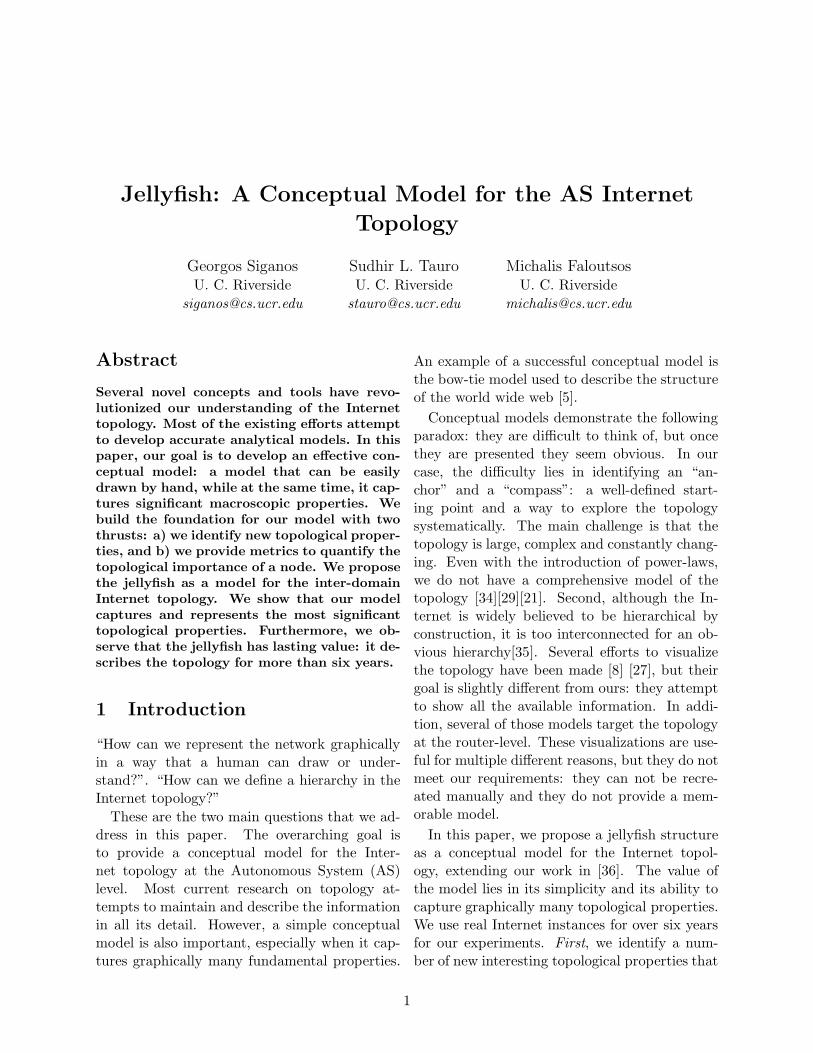
Figure 2: The logarithm of relative significanceversus the effective eccentricity for Int-07-2003.
we propose three metrics. The degree of a node isa straightforward metric of the importance. Nat-urally, a high degree suggests higher importance.Additionally, we explore the meaning and the re-lationships between the eccentricity and the sig-nificance.
The degree and the significance capturedifferent topological properties. The degreeand the significance are related, but at the sametime, they capture significantly different aspectsof the topology. The degree of a node capturesthe quantity of the neighbors, while the signifi-cance considers also the “quality” of the neigh-bors. For example, if we order the nodes accord-ing to significance and according to degree weobtain two drastically different sequences. Here,we will limit ourselves to an indicative example.In graph Int-11-97, we have a node with degree3 and significance 103.7, and a node of degree 10and significance 1.305. The first node4 connectsto the three most significant nodes of the graph,while the second node does not connect to anynode of high significance.
Significant nodes tend to be in the cen-ter of the network. The significance and theeffective eccentricity are correlated. In figure 2,
(amount of traffic that goes through a node).4Note that significance here is according to our defi-
nition, and captures the topological significance and notthe role of the node in the forwarding of traffic.
4

1
10
100
1000
1 10 100 1000 10000
Ave
rage
num
ber
of o
ne d
egre
e no
des
degree
’Int-07-2003’
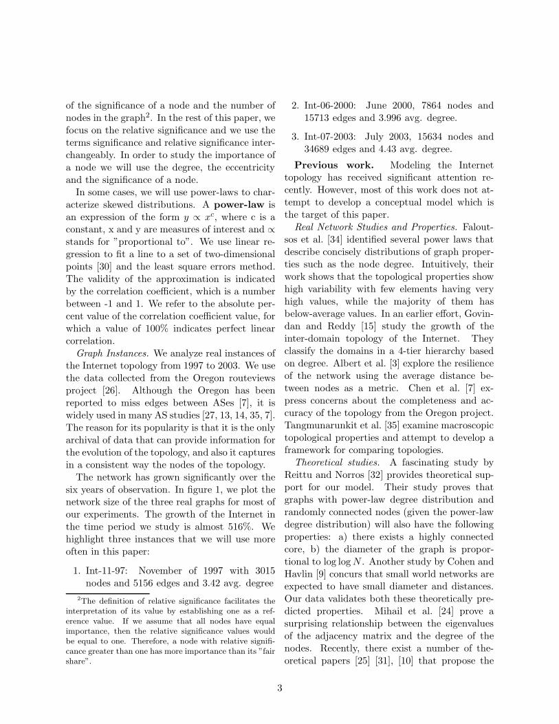
Figure 3: The average number of one-degreeneighbors versus the degree of such node.
we plot the logarithm of the significance versusthe effective eccentricity. We observe that nodesof high significance tend to have low effectiveeccentricity.Intuitively, this can be seen in twoways: central nodes are also significant, or thatsignificant nodes gravitate towards the center.
The effective eccentricity of adjacentnodes cannot differ by more than one.
Lemma 1 Let G=(V, E) be a connected undi-rected graph and (u, v) an edge in E, then theeffective eccentricity of nodes u and v can notdiffer by more than one:
|ecc(u) − ecc(v)| ≤ 1
This lemma is easy to prove, since for any nodex that node u can reach in h hops, node v canreach it with at most h + 1 hops.
This lemma helps us interpret the differencebetween the eccentricity of adjacent nodes. Wecan estimate the position of adjacent nodes withrespect to the center of the network. When doesthis maximum difference in eccentricity appear?It does, when all paths are passing through anode. For example, consider a node of degreeone: its eccentricity is equal to the eccentricityof its single neighbor plus one. We will refer tothis observation when we evaluate the model wedevelop.
0.0001
0.001
0.01
0.1
1
1 10 100 1000
CC
DF
One degree nodes connectivity
"2003.ccdf.one"linear fit
Figure 4: The CCDF of the one-degree neighborsof a node in log-log scale.
3.1 Location of One-Degree Nodes
The most common way to picture a hierarchy isto think of a social or military structure, whereeach class member connects to nodes of compa-rable importance. Each class connects to an im-mediately higher and lower class. Please refer toappendix B for a more detailed discussion on thismodel, which we call the cast or broom model.It turns out that the Internet topology deviatessignificantly from such a hierarchical model.
One-degree nodes are scattered all overthe network. We examine the spatial distri-bution of the one-degree nodes in the graph.Note that one-degree nodes, are approximately35 − 45% of the nodes. In figure 3, we plot theaverage number of one degree nodes, that are ad-jacent to a node, versus it’s degree. The qualita-tive observation is that one-degree nodes connectto both high and low degree nodes. Namely, theconnectivity is not selective on the degree: nodesof the lowest degree can connect directly to thetop nodes.
To better understand and characterize the onedegree nodes, we examine the distribution of theone degree neighbors of a node. We use theComplementary Cumulative Distribution Func-tion (CCDF) of the one degree neighbors of anode, which we denote as Or. We plot the Or
versus the number of one degree neighbors r inlog-log scale in figure 4 for graph Int-07-2003.
5
10
20
30
40
50
60
70
80
90
100
1997 2000 2003
Per
cent
age
of n
odes
rea
ched
Date
’hop.1’’hop.2’’hop.3’’hop.4’’hop.5’
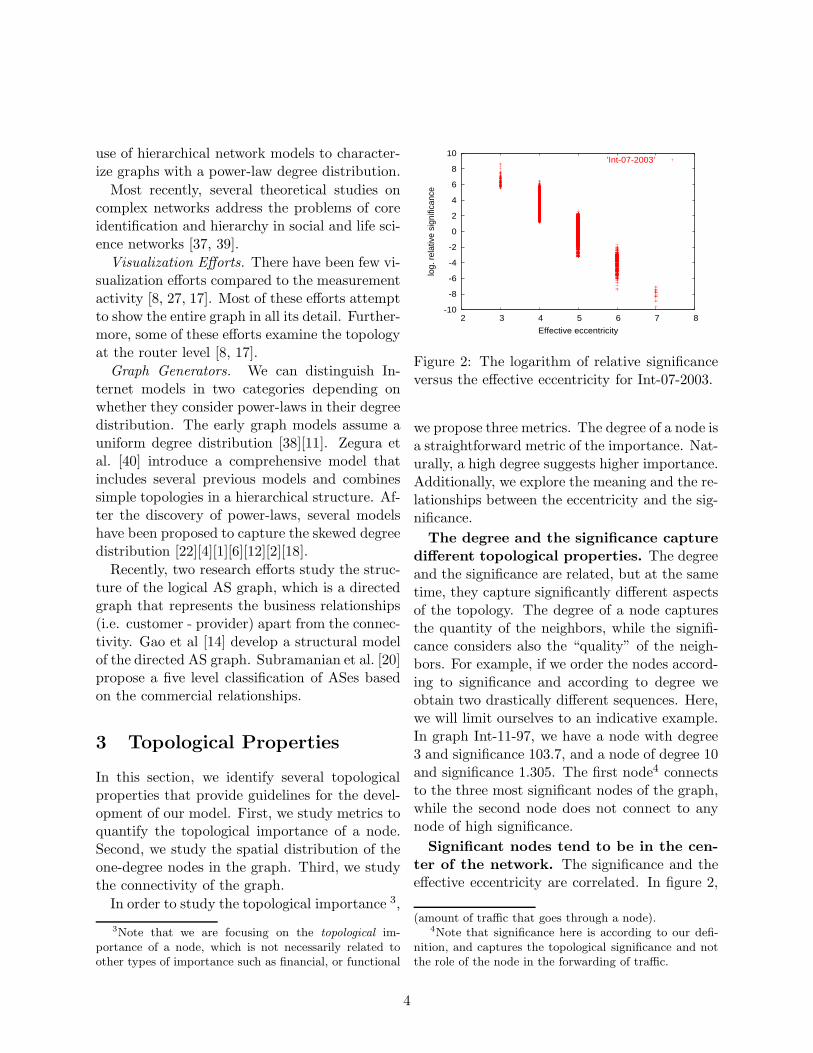
Figure 5: Percentage of nodes reached versusdate for the topological paths. Each line repre-sents the percentage for different number of hops.
The correlation coefficient is 99.5% for this in-stance and above 98% for all the instances weexamined. This observation can be stated as thefollowing power-law.
Power Law 4: Given a graph, the CCDFOr of the one degree neighbors r of a node, isproportional to the r to the power of a constantθ.
Or ∝ rθ
A natural question to ask, is whether thispower-law relates to the power-law of the de-gree distribution. Although there is a correlationbetween the degree of a node and the numberof its one-degree neighbors, we do not observea straightforward relationship such as a propor-tionality.
3.2 The Network Connectivity
To further examine the structure, we quantifythe connectivity with two complementary met-rics: a) the topological distances of the graph,b) the number of alternative paths that exist be-tween two nodes.
Topological distances. The distribution ofthe topological distances has remained practi-cally the same. We find that the distances in thenetwork do not change significantly in the time
1
10
100
1000
1 10 100
log
CC
DF
dest
ribut
ion
of n
umbe
r of p
aths
log path length
Number of pathslinear fit
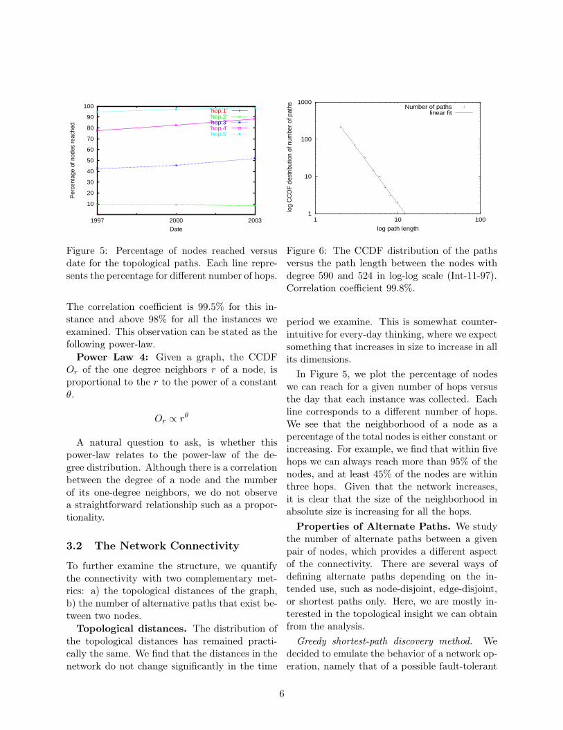
Figure 6: The CCDF distribution of the pathsversus the path length between the nodes withdegree 590 and 524 in log-log scale (Int-11-97).Correlation coefficient 99.8%.
period we examine. This is somewhat counter-intuitive for every-day thinking, where we expectsomething that increases in size to increase in allits dimensions.
In Figure 5, we plot the percentage of nodeswe can reach for a given number of hops versusthe day that each instance was collected. Eachline corresponds to a different number of hops.We see that the neighborhood of a node as apercentage of the total nodes is either constant orincreasing. For example, we find that within fivehops we can always reach more than 95% of thenodes, and at least 45% of the nodes are withinthree hops. Given that the network increases,it is clear that the size of the neighborhood inabsolute size is increasing for all the hops.
Properties of Alternate Paths. We studythe number of alternate paths between a givenpair of nodes, which provides a different aspectof the connectivity. There are several ways ofdefining alternate paths depending on the in-tended use, such as node-disjoint, edge-disjoint,or shortest paths only. Here, we are mostly in-terested in the topological insight we can obtainfrom the analysis.
Greedy shortest-path discovery method. Wedecided to emulate the behavior of a network op-eration, namely that of a possible fault-tolerant
6
routing protocol. Such a protocol may select theshortest path as primary path, and the secondshortest path as back up. We restrict the back uppath to be node disjoint with the primary. Fol-lowing this, in our study, for each pair of nodes,we iteratively find and remove the shortest path,except the end points. We stop when we cannotfind any more paths. Note that we have also con-sidered another approach based on the max-flowmethod, where we maximize the number of al-ternate node-disjoint paths, but the results werecomparable and are not shown here.
We find that the relationship between thenumber of node-disjoint paths and path lengthbetween a pair of nodes u and v is skewed. Infigure 6, we plot the relationship between theCCDF distributions of the number of paths ver-sus the path length for a pair of nodes. Wewant to capture this skewed path distributionconcisely in a qualitative way. This leads us tostate the following power-law as a rough approx-imation of the above observations. Recall thatour focus is the topological structure and not anaccurate model for the path length distribution.
Approximation Power Law 5: The com-plementary cumulative distribution function ofthe number of paths Ru,v of length lu,v betweena pair of nodes u and v (found by our greedyshortest path discovery method) is inversely pro-portional to the length of that path lu,v to thepower of a constant m.
Ru,v ∝ l−mu,v
The failure of the doughnut model. Thevalue of the above observation is its insight onthe macroscopic structure of the topology. Letus assume that the Internet topology is like aroughly homogeneous “doughnut”, which we dis-cuss further in appendix B. In this model, forany two nodes we would have two equally popu-lar path lengths, each corresponding to one sideof the doughnut. In that case, the path lengthdistribution would not follow the power-law weobserve in practice.
4 The Jellyfish Model
In this section, we integrate all the observationsand insight of the previous sections into a con-ceptual model. First, we identify a topologicalcenter and we classify nodes into layers with re-spect to the center. Then, we show how the jel-lyfish model captures all the properties that weexamined.
4.1 Core, Layers and Hierarchy
The first step in defining a hierarchy is to iden-tify a starting point. A natural point to look fora center is the most important node. In fact,we observe that the highest degree nodes are ad-jacent to each other. We define the core as aclique of high-degree nodes with the follow-ing procedure. We sort nodes in non-increasingdegree order. We select the highest degree nodeas the first member of the core. Then, we exam-ine each node in that order; a node is added tothe core only if it forms a clique with the nodesalready in the core. In other words, the new nodemust connect to all the nodes already in the core.We stop when we can not add any more nodes.This way, the core is a clique but not necessarilythe maximal clique of the graph.
Why do we define the core as a clique? Intu-itively, the clique makes the representation moreuseful when we consider node distances, and inparticular we can prove easily upper bounds forthe distances of two nodes, as we discuss later insection 4.2. A path passing from the clique willhave at most one hop through the clique. Thus,the distance between two nodes is bounded fromtheir relative from the clique plus the one hop inthe clique. In appendix A, we explore alternativedefinitions for the core by relaxing the stringentclique requirement. Recent, a work by Bar et al.examines the definition of an Internet core [33].
We now classify the rest of the nodes accordingto their proximity to the core. We define the firstlayer to be all the nodes adjacent to the core.Similarly, we define the second layer as the non-labeled neighbors of the first layer. By repeating
7
-12
-10
-8
-6
-4
-2
0
2
4
6
8
10
Core Layer-1 Layer-2 Layer-3 Layer-4 Layer-5
Effective Eccentricity
Log Relative Significance
Log degree
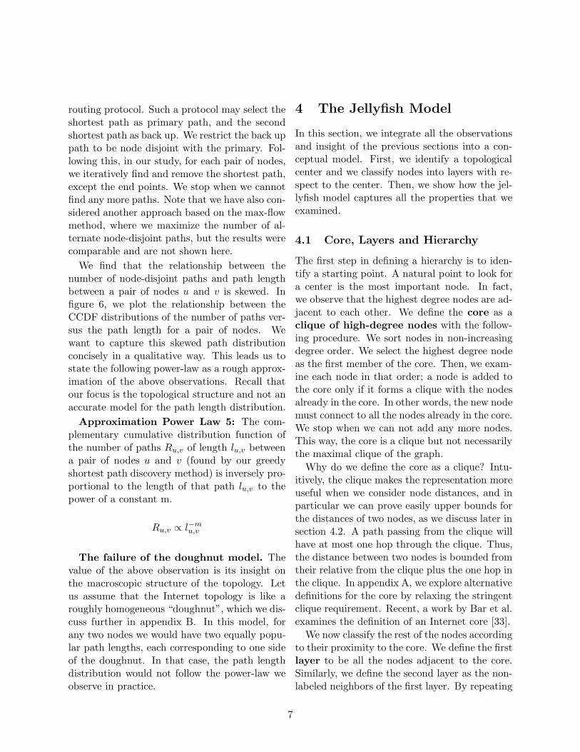
Figure 7: The average importance of each layer:log of the average degree, average effective eccen-tricity and log of the average relative significance(Int-07-2003 instance)
this procedure, we identify six layers if we countthe core as a layer zero.
Node distribution across layers. Table 1 showsthe distribution of the nodes for three Internetinstances. The node distribution across layersdoes not seem to change significantly in the in-stances we examine. We make two interestingobservations:
• Approximately 80-90% of the nodes are inthe first 3 layers.
• We find six layers in all the instances weexamine, and despite the significant networkgrowth.
These two observations strongly suggest that thenetwork grows “horizontally” by populating itslayers and not by adding more layers. We elab-orate on this point in the next section.
The effectiveness of the classification.We want to examine the effectiveness of our clas-sification and explore its topological meaning.First, we find that the layers differ significantlyin topological importance, which indicates thatthe classification captures some elements of thetopological structure. We use our three metricsto quantify the importance of each layer. Figure7 shows the average values of the effective eccen-tricity, the logarithm of the degree, and the log-
-6
-4
-2
0
2
4
6
8
10
Core Shell-1 Shell-2 Shell-3 Shell-4
Effective Eccentricity
Log Relative Significance
Log degree
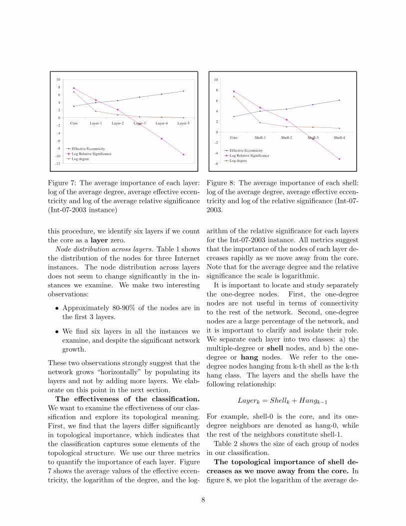
Figure 8: The average importance of each shell:log of the average degree, average effective eccen-tricity and log of the relative significance (Int-07-2003.
arithm of the relative significance for each layersfor the Int-07-2003 instance. All metrics suggestthat the importance of the nodes of each layer de-creases rapidly as we move away from the core.Note that for the average degree and the relativesignificance the scale is logarithmic.
It is important to locate and study separatelythe one-degree nodes. First, the one-degreenodes are not useful in terms of connectivityto the rest of the network. Second, one-degreenodes are a large percentage of the network, andit is important to clarify and isolate their role.We separate each layer into two classes: a) themultiple-degree or shell nodes, and b) the one-degree or hang nodes. We refer to the one-degree nodes hanging from k-th shell as the k-thhang class. The layers and the shells have thefollowing relationship:
Layerk = Shellk + Hangk−1
For example, shell-0 is the core, and its one-degree neighbors are denoted as hang-0, whilethe rest of the neighbors constitute shell-1.
Table 2 shows the size of each group of nodesin our classification.
The topological importance of shell de-creases as we move away from the core. Infigure 8, we plot the logarithm of the average de-
8
InstanceInt-11-1997 Int-06-2000 Int-07-2003
Layer No Nodes % of Nodes Nodes % of Nodes Nodes % of Nodes
Core/Layer-0 8 0.23 14 0.176 13 0.08
Layer-1 1354 44.90 3659 46.25 7330 46.27
Layer-2 1202 39.866 3090 39.05 7116 45.51
Layer-3 396 13.134 1052 13.29 1078 6.89
Layer-4 43 1.425 86 10.87 96 0.61
Layer-5 12 0.398 10 0.12 1 0.0063
Table 1: Distribution of nodes in layers for three Internet instances.
InstanceInt-11-1997 Int-06-2000 Int-07-2003
Layer ID Nodes % of Nodes Nodes % of Nodes Nodes % of Nodes
Core/Shell-0 8 0.23 14 0.176 13 0.08
Hang-0 465 15.42 798 10.08 1174 7.5
Shell-1 889 29.49 2861 36.16 6156 39.37
Hang-1 623 20.66 1266 16 2821 18.04
Shell-2 579 19.2 1824 23.05 4295 27.47
Hang-2 299 9.92 662 8.36 808 5.16
Shell-3 97 3.22 390 4.92 270 1.72
Hang-3 41 1.36 74 0.93 84 0.53
Shell-4 2 0.66 12 0.15 12 0.07
Hang-4 12 0.4 10 0.12 1 0.006
Table 2: Distribution of nodes in shell and hang classes.
9
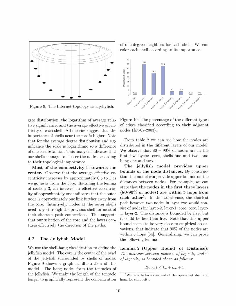
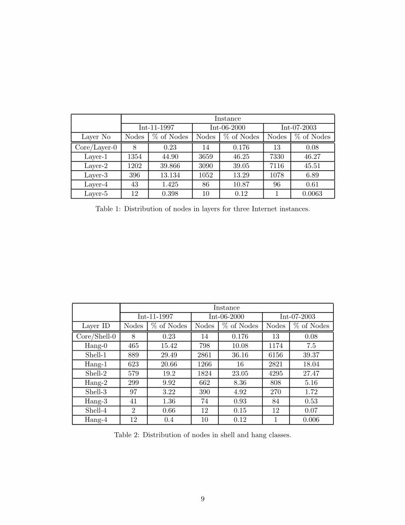
Figure 9: The Internet topology as a jellyfish.
gree distribution, the logarithm of average rela-tive significance, and the average effective eccen-tricity of each shell. All metrics suggest that theimportance of shells near the core is higher. Notethat for the average degree distribution and sig-nificance the scale is logarithmic so a differenceof one is substantial. This analysis indicates thatour shells manage to cluster the nodes accordingto their topological importance.
Most of the connectivity is towards thecenter. Observe that the average effective ec-centricity increases by approximately 0.5 to 1 aswe go away from the core. Recalling the lemmaof section 3, an increase in effective eccentric-ity of approximately one indicates that the outernode is approximately one link further away fromthe core. Intuitively, nodes at the outer shellsneed to go through the previous shell for most oftheir shortest path connections. This suggeststhat our selection of the core and the layers cap-tures effectively the direction of the paths.
4.2 The Jellyfish Model
We use the shell-hang classification to define thejellyfish model. The core is the center of the headof the jellyfish surrounded by shells of nodes.Figure 9 shows a graphical illustration of thismodel. The hang nodes form the tentacles ofthe jellyfish. We make the length of the tentaclelonger to graphically represent the concentration
of one-degree neighbors for each shell. We cancolor each shell according to its importance.
0.22
34.8
24.5
32.5
3.7 3.7
0.12 0.30
5
10
15
20
25
30
35
40
Cor
e to
Cor
e
Cor
e to
Lay
er-1
Layer
-1 to
Lay
er-1
Layer
-2 to
Lay
er-2
Layer
-2 to
Lay
er-3
Layer
-3 to
Lay
er-3
Layer
-3 to
Lay
er-4
Layer
-1 to
Lay
er-2
Per
cen
tag
e o
f E
dg
es
Figure 10: The percentage of the different typesof edges classified according to their adjacentnodes (Int-07-2003).
From table 2 we can see how the nodes aredistributed in the different layers of our model.We observe that 80 − 90% of nodes are in thefirst few layers: core, shells one and two, andhang one and two.
The jellyfish model provides upperbounds of the node distances. By construc-tion, the model can provide upper bounds on thedistances between nodes. For example, we canstate that the nodes in the first three layers(80-90% of nodes) are within 5 hops fromeach other5. In the worst case, the shortestpath between two nodes in layer two would con-sist of nodes in: layer-2, layer-1, core, core, layer-1, layer-2. The distance is bounded by five, butit could be less than five. Note that this upperbound seems to be very close to empirical obser-vations, that indicate that 90% of the nodes arewithin 5 hops [34]. Generalizing, we can provethe following lemma.
Lemma 2 (Upper Bound of Distance):The distance between nodes v of layer-kv and w
of layer-kw is bounded above as follows:
d(v,w) ≤ kv + kw + 1
5We refer to layers instead of the equivalent shell andhang for simplicity.
10

The proof is a straightforward if we considerthe construction of the layers.
In the jellyfish model, 70% of edges arebetween different node layers. In Figure 10we plot the percentage of edges that exist be-tween and within layers. We find that 70% ofthe edges connect nodes between different lay-ers. We think of these edges as vertical withrespect to the jellyfish hierarchy. In contrast,approximately 30% are horizontal to the hierar-chy providing connectivity between nodes of thesame class.
Let us examine the vertical edges in more de-tail. The construction of the jellyfish model is abreadth-first type of network exploration. Thebreadth-first tree consists of N − 1 edges, whereN the number of nodes. The number of edgesin the graph is approximately: 2N (average de-gree close to four). Therefore, 50% of the edgesare part of the breadth first tree of the jellyfish.Recall that 70% of the edges are vertical edges.This means that the other 70− 50 = 20% of thevertical edges are “redundant” edges.
Why is the jellyfish a good model? It should beclear by now that this model is driven by severalempirical observations. We provide an overviewof the topological properties that the jellyfishmodel captures. As an intuitive model, the jel-lyfish represents these properties in a graphicaland qualitative way6.
1. Core: The topology has a core of highlyconnected topologically-important nodes,which is represented by the center of the jel-lyfish cap.
2. Five layers: The distances between nodesare small; maximum distance less than 11hops, and 80% of nodes are within 5 hops.
3. Center-heavy: 80% of the nodes are in thefirst 3 layers.
6Note that not all properties listed below can be de-duced directly from the model, but the model can act asa intuitive reminder.
Core Hang-0 Shell1 Hang-1 Shell2 Hang-2 Shell3 Hang-3 Shell4 Hang-4 0
5
10
15
20
25
30
35
% o
f tot
al g
raph
shell/hang
8/11/1997 4/30/1998 8/1/1998 11/30/1998 4/30/1999 7/15/1999 10/10/1999 Jun-00
Figure 11: The distribution of nodes over timegrouped by class.
4. One-degree nodes: There is a non-trivialpercentage (35-45%) of one-degree nodes,which are scattered everywhere (represen-tation of power-law 4).
5. The importance of the nodes decreases withtheir distance from the core.
6. The model provides good upper bounds ofthe distances between nodes.
An additional strength of the model is thatit has persisted in time. Its structure and thenode distribution across classes has not changedqualitatively during the years of our study. Weelaborate on the model evolution in the next sec-tion.
5 The Evolution of the Jellyfish
We study the evolution of the Internet struc-ture for approximately three years. We find thatthe statistical properties of the jellyfish modelchange relatively little over time. Second, we findthat the node and edge distribution across thejellyfish classes remains approximately the same.Third, we find that the classification of individ-ual nodes does not change significantly within athree to eight month interval. Finally, we studythe identity of the nodes that constitute the core.
11
Nov97 Apr98 Nov98 Apr99 July99 Oct99v/s v/s v/s v/s v/s v/s
Apr98 Aug98 Apr99 July99 Oct99 June00
No change 1845 2829 3278 3986 4289 3972
Total change 968 651 887 919 963 1615
Hang to shell 343 228 395 312 320 634
Shell to hang 148 155 227 193 265 382
Drop in shell 119 69 97 152 54 256
Increase in shell 117 97 60 62 171 140
Drop in hang 91 38 67 155 27 125
Increase in hang 150 64 41 45 126 78
Table 3: The change in the node classification between consecutive instances.
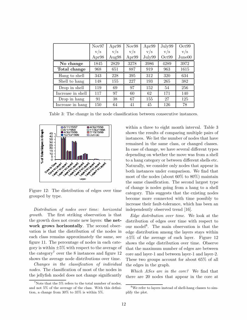
Figure 12: The distribution of edges over timegrouped by type.
Distribution of nodes over time: horizontalgrowth. The first striking observation is thatthe growth does not create new layers: the net-work grows horizontally. The second obser-vation is that the distribution of the nodes ineach class remains approximately the same, seefigure 11. The percentage of nodes in each cate-gory is within ±5% with respect to the average ofthe category7 over the 8 instances and figure 12shows the average node distributions over time.
Changes in the classification of individualnodes. The classification of most of the nodes inthe jellyfish model does not change significantly
7Note that the 5% refers to the total number of nodes,and not 5% of the average of the class. With this defini-tion, a change from 30% to 35% is within 5%.
within a three to eight month interval. Table 3shows the results of comparing multiple pairs ofinstances. We list the number of nodes that haveremained in the same class, or changed classes.In case of change, we have several different typesdepending on whether the move was from a shellto a hang category or between different shells etc.Naturally, we consider only nodes that appear inboth instances under comparison. We find thatmost of the nodes (about 60% to 80%) maintainthe same classification. The second largest typeof change is nodes going from a hang to a shellcategory. This suggests that the existing nodesbecome more connected with time possibly toincrease their fault-tolerance, which has been anindependently observed trend [16].
Edge distribution over time. We look at thedistribution of edges over time with respect toour model8. The main observation is that theedge distribution among the layers stays within±5% of the average of each layer. Figure 12shows the edge distribution over time. Observethat the maximum number of edges are betweencore and layer-1 and between layer-1 and layer-2.These two groups account for about 65% of allthe edges in the graph.
Which ASes are in the core? We find thatthere are 20 nodes that appear in the core at
8We refer to layers instead of shell-hang classes to sim-plify the plot.
12

least once in the eight instances we examine.Among them, only four nodes appear in all eightinstances. The maximum number of nodes in thecore in any instance was 14 and the minimumwas 8. Here are the most interesting observa-tions:
• The maximum number of nodes in the coreis 14 in June 2000, while the minimum is 8in November 1997 and August 1998.
• There were four nodes that are always in thecore: AlterNet, Cable and Wireless, Sprint-Link and GTE Internetworking. Thesenodes also constitute the highest-degreenodes in the core, except in June 2000 whenAT&T (572) exceeded GTE (426)
• The node with the smallest degree in thecore was Exodus communications (53) inApril 1998.
6 The Importance of the Jelly-
fish Model
So far, we showed that the jellyfish can be used todescribe the Internet in a consistent way for thelast six years. In this section, we demonstratethe usefulness of jellyfish. There are two param-eters that we need to investigate. First, we try toanswer whether all graphs can be described us-ing the jellyfish model that we found in the pre-vious sections. Ideally, jellyfish should be able todistinguish among different type of graphs. Wetry to answer this in a qualitative way by us-ing simple regular topologies, and we show thatnot all topologies can be characterized as jelly-fish. Second, we check whether our model canbe used to distinguish among power-law graphs9.Using two popular graph generators, we showthat graphs that follow approximately the samepower-law distribution, can have significant dif-ferent macroscopic properties, and can be distin-guished using jellyfish.
9By power-law graphs, we mean graphs that their de-gree distribution follows a power-law
Can any graph be modeled as a jellyfish?For every graph, we can pick a center and com-pute it’s layers. On the other hand, not everygraph can match the Internet profile, i.e. thenumber of layers and the distribution of nodesamong these layers. For example, let us considersome regular topologies such as a square mesh, acomplete binary (or k-ary) tree, a clique 10, andpurely random graphs. None of these graphs willfit the above description of the jellyfish in all itsaspects. As an example, we will mention a few ofthe more pronounced differences. First, there isno natural central point to place the core. Evenif we define an arbitrary core, there are also otherproperties that will be violated. The mesh andthe tree will have a large number of shells propor-tional to O(
√N) or O(log N) respectively. More
importantly, when the size of the network woulddouble, the number of layers and shells would in-crease, which does not happen here. The cliquealso does not fit the jellyfish profile: it has onlyone layer, and no one-degree nodes. We havealso seen other network models which do notmatch this profile such as the strictly hierarchicalmodel, and the doughnut model in appendix B.
6.1 Power-law Graph Generators
We can use the Jellyfish model as a test of therealism of Internet like graphs. We will usethe GLP methodology proposed in [6], and thePLRG approach proposed in [1]. The GLP ap-proach depends on the preferential model, and itis the most recent proposed generator and is con-sidered to be the state of the art. On the otherhand, the PLRG generator is based on an in-teresting theoretical model for scale free graphs,and takes the degree distribution as a given.Note that in [6], they compared the two gen-erators and found that the best generator is theGLP. They showed that PLRG fails to captureproperties like the characteristic path length andthe clustering coefficient. We show that GLP
10Varying these models by adding or removing a fewedges or nodes in a uniformly distributed way will notreconciliate the differences with the jellyfish in most cases.
13

InstanceGLP Int-06-2000 PLRG
Layer ID Nodes % of Nodes Nodes % of Nodes Nodes % of Nodes
Core/Shell-0 21 0.2 14 0.176 11 0.13
Hang-0 1885 23.82 798 10.08 565 7.1
Shell-1 1672 21.13 2861 36.16 2346 29.6
Hang-1 3371 42.6 1266 16 1298 16.4
Shell-2 688 8.7 1824 23.05 2305 29.13
Hang-2 221 2.79 662 8.36 525 6.6
Shell-3 3 0.037 390 4.92 325 4.1
Hang-3 3 0.037 74 0.93 125 1.5
Shell-4 0 0 12 0.15 41 0.51
Hang-4 0 0 10 0.12 23 0.29
Table 4: Distribution of nodes in shell and hang classes.
does not capture the macro structure that wefound using jellyfish. Incidentally, PLRG seemsto pass the test, although it fails other proper-ties. Therefore, our jellyfish model is an excellenttool to distinguish graphs.
We use the Brite generator [23] for the GLPmodel, which includes an implementation of thismodel 11. We have implemented PLRG. In orderto compare the Internet topology with the gen-erators, we will use the Int-06-2000 graph. Wewant to generate a topology that would have thesame properties as Int-06-2000. Following themethodology presented in [6] we use the follow-ing parameters: ρ = 0.434 and β = 0.661 for theGLP. For the PLRG, we simply use the degreedistribution of Int-06-2000.
The correlation coefficient for the degreepower-law plot is 97, 6% for the GLP with slopea = −1.092. For the PLRG plot the correlationcoefficient is 99, 7% and the slope is a = −1.243.For the Int-06-2000 the correlation coefficient is99.7% and the slope is a = −1.16312. In table 4,
11Note that the GLP model in the Brite generator isnot exactly the same as described in the original paper.The difference lies in that the number of edges of a newnode can be either one with probability 87%, or two withprobability 13%. We updated the model used in brite toreflect the original approach.
12Note that the PLRG doesn’t have the exact samedegree distribution as the Int-06-2000. When we generate
we have the decomposition of the graphs usingthe jellyfish model. These results clearly showthat the generated graph using the GLP method-ology is qualitatively different than the Internetgraph. On the other hand PLRG seems to main-tain similar structure according to the jellyfishmodel. The only differences between PLRG andInt-06-2000 is that the clique is smaller, havingonly 11 nodes, and that we have a slightly smallershell-1 and bigger shell-2.
Where does GLP fail to model the In-ternet? The main differences between GLP andthe Int-06-2000 can be summarized as following:
1. The core of the network is much bigger inGLP compared to the Internet. More specif-ically, we have 21 nodes in the core for theGLP, while only 14 nodes in the Int-06-2000.
2. The number of hanging nodes (degree one)far out-exceeds the number of shell nodes.The analogy is approximately 70% hangingnodes to 30% shell nodes. In the case of theInt-06-2000 we have the opposite result.
3. The GLP topology has only up to 5 layers,with the 5th layer having only 3 members,
the topology using PLRG, we might pick to connect twonodes that are already connected, so in this sense we havefewer edges in the final graph.
14

while the Int-06-2000 has 6 layers.
Using our analysis we can conclude that jellyfishis an excellent tool to distinguish among genera-tors into two classes, those that can capture themacro structure of the Internet and those thatcan not.
7 Conclusions
In this paper, we develop a simple and concep-tual topological model for the inter-domain In-ternet topology. Our work has five componentsof independent interest. First, we present andstudy three metrics of the topological impor-tance of a node. Second, we identify some newtopological properties. Third, we integrate themain properties into our jellyfish model. Fourth,we study the time evolution of the Internet withrespect to our model. Finally, we show that ourmodel can be used to distinguish among graphgenerators.
The jellyfish model provides novel insight intothe structure of the Internet topology. Despiteits simple nature, the jellyfish captures most ofthe known macroscopic properties. The modelfacilitates the visualization of the complex Inter-net structure by abstracting it into somethingthat a human can easily picture and understand.
We summarize our main observations and con-tributions in the following points.
• We use three metrics to quantify the topo-logical importance of a node and we examinetheir meaning and their relationships.
• The Internet has a highly connected coreand layers of nodes in decreasing impor-tance. This way, we can define a notion ofloose hierarchy in the network.
• The jellyfish model provides fairly tight up-per bounds of the distances between nodes.
• Low degree nodes are scattered in the net-work in contrast to a strictly layered hierar-chy.
• Approximately 30% of the edges are be-tween nodes of the same class according toour model. From the remaining edges, 20%of the edges are “redundant” edges betweenadjacent layers.
• The topological growth is horizontal: thenumber of layers has not increased overtime.
• The statistical properties of the topol-ogy with respect to the jellyfish have notchanged significantly over time.
• The jellyfish can be used to distinguishamong graph generators.
In the future, we want to develop a theoreticalframework that will explain and justify our ex-perimentally derived model. The ground break-ing work of Reittu and Norros [32] opens thedoors for a parallel approach where theory andreal-data analysis complement each other. Fur-thermore, we intend to elaborate and fine tunethe jellyfish model by integrating more topolog-ical properties. We want to identify more topo-logical properties and integrate them into themodel using novel means such as color. Finally,we want to examine whether other real networkscan be described by the jellyfish model.
References
[1] W. Aiello, F. Chung, and L. Lu. A random graphmodel for massive graphs. STOC, pages 171–180, 2000.
[2] R. Albert and A. Barabasi. Topology ofcomplex networks:local events and universality.Phys.Review Letters, 85, 5234, 2000.
[3] R. Albert, H. Jeong, and A. Barabasi. Attackand error tolerance of complex networks. Nature,406, 378, July 2000.
[4] A. Barabasi and R. Albert. Emergence of scal-ing in random networks. Science, 286, 509-512,October 1999.
[5] A. Broder, R. Kumar, F. Maghoul, P. Ragha-van, S. Rajagopalan, R. Stata, A. Tomkins, and
15

J. Wiener. Graph structure in the web: exper-iments and models. In Proc. of the 9th WorldWide Web Conference, 2000.
[6] T. Bu and D. Towsley. On distinguishing be-tween Internet power law topology generators.IEEE Infocom, 2002.
[7] Qian Chen, Hyunseok Chang, Ramesh Govin-dan, Sugih Jamin, Scott J. Shenker, and WalterWillinger. The origin of power laws in Internettopologies revisited. IEEE Infocom, 2001.
[8] Bill Cheswick and Hal Burch. Inter-net mapping project. Wired Maga-zine, December 1998. See http://cm.bell-labs.com/cm/cs/who/ches/map/index.html.
[9] Reuven Cohen and Shlomo Havlin. Scale-freenetworks are ultrasmall. Physical Letters Re-view, 90(5), 2002.
[10] F. Comellas, G. Fertin, and A. Raspaud. Ver-tex labeling and routing in recursive clique-trees,a new family of small-world scale-free graphs.Sirocco, 2003.
[11] M. Doar. A better model for generating testnetworks. IEEE Global Internet, Nov. 1996.
[12] A. Fabrikant, E. Koutsoupias, and C.H. Pa-padimitriou. Heuristically optimized trade-offs:A new paradigm for power laws in the Internet.ICALP, Springer-Verlag LNCS:110–122, 2002.
[13] Lixin Gao. On inferring automonous system re-lationships in the Internet. IEEE/ACM Trans-actions on Networking, 9:733–745, December2001.
[14] Z. Ge, D. Figueiredo, S. Jaiswal, and L. Gao. Onthe hierarchical structure of the logical internetgraph. SPIE ITComm, 2001.
[15] R. Govindan and A. Reddy. An analysis of In-ternet Inter-domain topology and route stability.IEEE Infocom, Kobe, Japan, April 7-11 1997.
[16] Geoff Huston. Homepage:.http://www.telstra.net/gih, 2001.
[17] Young Hyun. Walrus project.http://mappa.mundi.net/maps/maps 020/,2002.
[18] Cheng Jin, Qian Chen, and Sugih Jamin. Inet:Internet topology generator. Techical ReportUM CSE-TR-433-00, 2000.
[19] J. Kleinberg. Authoritative sources in a hyper-linked environment. Journal of the ACM, 1999.(Earlier version in ACM-SIAM Symposium onDiscrete Algorithms, 1998).
[20] L.Subramanian, S.Agarwal, J.Rexford, andR.Katz. Characterizing the Internet hierarchyfrom multiple vantage points. IEEE Infocom,2002.
[21] Damien Magoni and Jean Jacques Pansiot.Analysis of the autonomous system networktopology. ACM Sigcomm Computer Communi-cation Review, 31(3):26–37, July 2001.
[22] A. Medina, I. Matta, and J. Byers. Onthe origin of powerlaws in Internet topologies.ACM Sigcomm Computer Communication Re-view, 30(2):18–34, April 2000.
[23] Alberto Medina, Anukool Lakhina, IbrahimMatta, and John Byers. BRITE: Topology gen-erator. http://www.cs.bu.edu/brite/.
[24] M.Mihail and C.H.Papadimitriou. On the eigen-value power law. Random, 2002.
[25] Jae Dong Noh. Exact scaling properties of ahierarchical network model. Physical Review E,67(045103), 2003.
[26] University of Oregon RouteViews Project. Online data and reports.http://www.routeviews.org/.
[27] CAIDA Org. Skitter project.http://www.caida.org/tools/measurement/skitter/,2002.
[28] C. Palmer, G. Siganos, M. Faloutsos, C. Falout-sos, and P. Gibbons. The connectivity andfault-tolerance of the Internet topology. Work-shop on Network-Related Data Management(NRDM 2001), In cooperation with ACM SIG-MOD/PODS, Santa Barbara, 2001.
[29] J.-J. Pansiot and D Grad. On routes and multi-cast trees in the Internet. ACM Sigcomm Com-puter Communication Review, 28(1):41–50, Jan-uary 1998.
[30] William H. Press, Saul A. Teukolsky, William T.Vetterling, and Brian P. Flannery. NumericalRecipes in C. Cambridge University Press, 2ndedition, 1992.
[31] Erzsebet Ravasz and Albert-Laszlo Barabasi.Hierarchical organization in complex networks.Physical Review E, 67(026112), 2003.
16
[32] H. Reittu and I. Norros. On the power law ran-dom graph model of the internet. Tech. Report,VTT Information Technology, 2002.
[33] M. Gonen S. Bar and A. Wool. An incremen-tal super-linear preferential internet topologymodel. 5th Annual Passive and Active Measure-ment Workshop (PAM), 2004.
[34] G. Siganos, M. Faloutsos, P. Faloutsos, andC. Faloutsos. Power-laws and the as-level Inter-net topology. IEEE/ACM Trans. on Network-ing, August 2003.
[35] H. Tangmurankit, R. Govindan, S. Jamin, S. J.Shenker, and W. Willinger. Network topologygenerators: Degree-based vs structural. ACMSigcomm, 2002.
[36] L. Tauro, C. Palmer, G. Siganos, and M. Falout-sos. A simple conceptual model for the internettopology. IEEE Global Internet, November 2001.
[37] K. W. Koput W. W. Powell, D. R. White andJ. Owen-Smith. Network dynamics and field evo-lution: The growth of interorganizational collab-oration in the life sciences. American Journal ofSociology, 110(4):1132–1205, 2005.
[38] B. M. Waxman. Routing of multipoint connec-tions. IEEE Journal of Selected Areas in Com-munications, pages 1617–1622, 1988.
[39] D. R. White, J. Owen-Smith, J. Moody, andW. W. Powell. Network dynamics and field evo-lution: The growth ofinterorganizational collab-oration in the life sciences. Computational andMathematical Organization Theory, 10(1):95–117, 2004.
[40] E. W. Zegura, K. L. Calvert, and M. J. Donahoo.A quantitative comparison of graph-based mod-els for internetworks. IEEE/ACM Transactionson Networking, 5(6):770–783, December 1997.http://www.cc.gatech.edu/projects/gtitm/.
A Core: Relaxing the clique
constraint
We explain our choice of defining our core to be aclique containing the maximal degree node. Onecould consider near-cliques, and include in thecore nodes of high degree that connect with al-most all the core nodes. This would make sense
0 2 4 6 8 10 12
0.00
0.02
0.04
0.06
0.08
0.10
0.12
0.14
0.16
Ave
rage S
ignifi
cance
Value of n
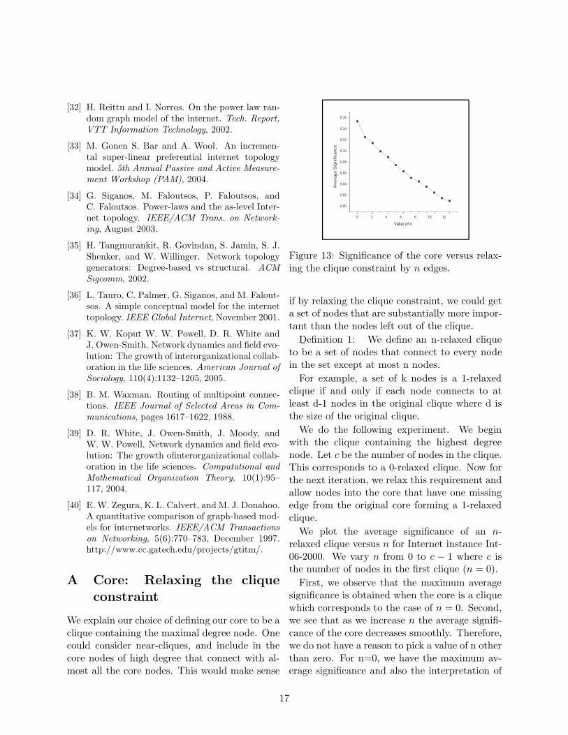
Figure 13: Significance of the core versus relax-ing the clique constraint by n edges.
if by relaxing the clique constraint, we could geta set of nodes that are substantially more impor-tant than the nodes left out of the clique.
D¯efinition 1: We define an n-relaxed clique
to be a set of nodes that connect to every nodein the set except at most n nodes.
For example, a set of k nodes is a 1-relaxedclique if and only if each node connects to atleast d-1 nodes in the original clique where d isthe size of the original clique.
We do the following experiment. We beginwith the clique containing the highest degreenode. Let c be the number of nodes in the clique.This corresponds to a 0-relaxed clique. Now forthe next iteration, we relax this requirement andallow nodes into the core that have one missingedge from the original core forming a 1-relaxedclique.
We plot the average significance of an n-relaxed clique versus n for Internet instance Int-06-2000. We vary n from 0 to c − 1 where c isthe number of nodes in the first clique (n = 0).
First, we observe that the maximum averagesignificance is obtained when the core is a cliquewhich corresponds to the case of n = 0. Second,we see that as we increase n the average signifi-cance of the core decreases smoothly. Therefore,we do not have a reason to pick a value of n otherthan zero. For n=0, we have the maximum av-erage significance and also the interpretation of
17
Property Cast Furball Doughnut Jellyfish
Horizontal Connectivity no yes yes yes
High-Low Degree Edges no no maybe yes
Distance Distribution yes yes no yes
Table 5: The matrix of observed properties and wether they are satisfied by the different models.
the core is straightforward.
B Failed Internet Models
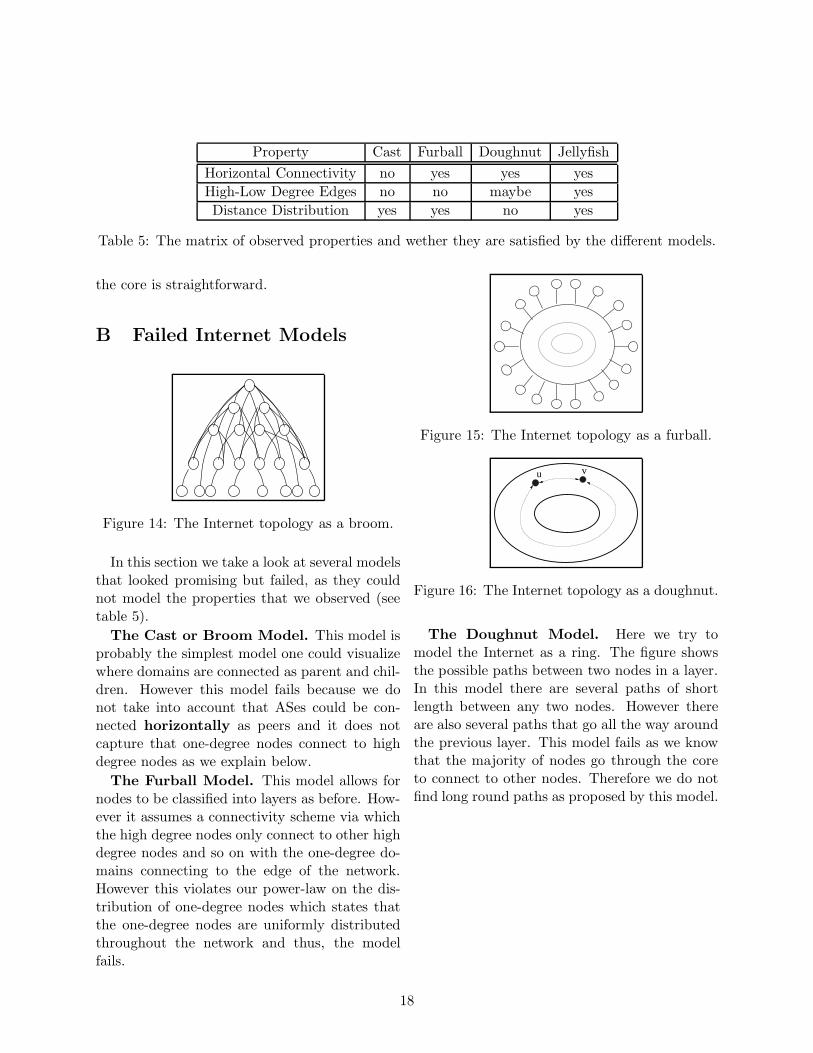
Figure 14: The Internet topology as a broom.
In this section we take a look at several modelsthat looked promising but failed, as they couldnot model the properties that we observed (seetable 5).
The Cast or Broom Model. This model isprobably the simplest model one could visualizewhere domains are connected as parent and chil-dren. However this model fails because we donot take into account that ASes could be con-nected horizontally as peers and it does notcapture that one-degree nodes connect to highdegree nodes as we explain below.
The Furball Model. This model allows fornodes to be classified into layers as before. How-ever it assumes a connectivity scheme via whichthe high degree nodes only connect to other highdegree nodes and so on with the one-degree do-mains connecting to the edge of the network.However this violates our power-law on the dis-tribution of one-degree nodes which states thatthe one-degree nodes are uniformly distributedthroughout the network and thus, the modelfails.
Figure 15: The Internet topology as a furball.
u v
Figure 16: The Internet topology as a doughnut.
The Doughnut Model. Here we try tomodel the Internet as a ring. The figure showsthe possible paths between two nodes in a layer.In this model there are several paths of shortlength between any two nodes. However thereare also several paths that go all the way aroundthe previous layer. This model fails as we knowthat the majority of nodes go through the coreto connect to other nodes. Therefore we do notfind long round paths as proposed by this model.
18