ORDINAL ANALYSIS WITHOUT PROOFS

JEREMY AVIGAD

Abstract. An approach to ordinal analysis is presented which is finitary, but high-

lights the semantic content of the theories under consideration, rather than the syntactic

structure of their proofs. In this paper the methods are applied to the analysis of the-

ories extending Peano arithmetic with transfinite induction and transfinite arithmetic

hierarchies.

§1. Introduction. As the name implies, in the field of proof theory onetends to focus on proofs. Nowhere is this emphasis more evident than inthe field of ordinal analysis, where one typically designs procedures for “un-winding” derivations in appropriate deductive systems. One might wonder,however, if this emphasis is really necessary; after all, the results of an ordinalanalysis describe a relationship between a system of ordinal notations and atheory, and it is natural to think of the latter as the set of semantic conse-quences of some axioms. From this point of view, it may seem disappointingthat we have to choose a specific deductive system before we can begin theordinal analysis.

In fact, Hilbert’s epsilon substitution method, historically the first attemptat finding a finitary consistency proof for arithmetic, has a more semantic char-acter. With this method one uses so-called epsilon terms to reduce arithmeticto a quantifier-free calculus, and then one looks for a procedure that assignsnumerical values to any finite set of closed terms, in a manner consistent withthe axioms. The first ordinal analysis of arithmetic using epsilon terms is dueto Ackermann [1]; for further developments see, for example, [20].

2000 Mathematics Subject Classification. 03F15,03F05,03F30.Dedicated to Solomon Feferman on the occasion of his 70th birthday.

It is an honor to be able to contribute a paper to this volume. Although I did my

graduate work under Jack Silver at Berkeley, Sol served as an informal second advisor tome, and his thoughtful advice and guidance made frequent visits to Stanford both enjoyable

and well worthwhile. Mathematical logic, as a discipline, is poised between philosophy and

mathematics, and so has to answer to competing standards of philosophical relevance andmathematical elegance. Throughout his career, Sol has been able to strike a harmonious

balance between the two, with work that is deeply satisfying on both counts. His style sets

a high standard for future generations, and one that many of us will look to as a model.I would like to thank Lev Beklemishev for comments and suggestions, and the anonymous

referees for their very careful readings.Work partially supported by NSF Grant DMS 9614851.

c© 2000, Association for Symbolic Logic 1

2 JEREMY AVIGAD

More recently, investigations of nonstandard models of arithmetic due toParis and Kirby have given rise to another approach, which incorporates Ke-tonen and Solovay’s finitary combinatorial notion of an α-large set of naturalnumbers. Roughly speaking, to show that the proof-theoretic ordinal of a the-ory T is bounded by α, one uses an α-large interval in a nonstandard modelof arithmetic to construct a model of T . These methods are surveyed andextended in [3, 4]; some of the constructions found in the second paper arederived from model-theoretic methods due to Friedman [12, 13]. Sommer [28]has shown that one can avoid references to nonstandard models and insteadview the methods as providing a way of building “finite approximations” tomodels of arithmetic, an idea which traces its way back to Herbrand [18]. (Seealso the introduction to [19].)

Finally, Quinsey has shown that a notion called fulfillment, due to Kripke,provides yet another way of using more semantic methods to obtain tradi-tional proof-theoretic results. His Ph.D. thesis [23] is a tour-de-force, offeringa wealth of applications in wide range of areas. Similar ideas have been devel-oped independently by Carlson [10].

Each of the approaches just described has its own advantages and disadvan-tages. But with their emphasis on “building models” over “unwinding proofs,”the similarities between them are more striking than the differences. And thepersistence with which this point of view keeps resurfacing suggests that suchmethods may have something to offer to the development of proof theory.

In this paper, I have tried to fashion an approach to ordinal analysis whichis in concord with these themes, incorporating and adapting ideas from allthe sources mentioned above. Since these ideas have appeared in so manydifferent contexts, often arising independently, trying to sort out the properaccreditations at each step along the way would be difficult; and so I hopethis broad attribution is enough to acknowledge the general debt that thiswork owes to that which has come before. I should mention that I have alsobenefited a good deal from Buss’ ordinal analysis of arithmetic, using thewitnessing method, in [7]; from the emphasis on ordinal recursion and itsproperties, in Friedman and Sheard [11]; and, of course, from the traditionalGentzen-Schutte approach to ordinal analysis, surveyed in [21, 22, 24].

One aspect of the approach developed here is that Herbrand’s theorem isused in a central way. One begins by embedding a classical theory in a uni-versal one, with symbols describing functions that are nonconstructive in theintended interpretation. By Herbrand’s theorem, to extract an appropriatewitness from the proof of a Σ1 sentence, one does not need to know the correctinterpretation of the function symbols; one only needs an interpretation thatis consistent with a finite set of axioms relevant to the proof.

Another aspect of the approach is that it is cumulative: once we have ana-lyzed a theory Tα, dependent on a parameter α, we can work “in” that theoryto analyze the next nonconstructive principle. That way, as we work our way

ORDINAL ANALYSIS WITHOUT PROOFS 3

up, we can leave behind the low-level combinatorial constructions, and carryon in a more familiar mathematical and logical framework.

Despite the semantic flavor of the approach, it is entirely finitary, in a sensethat will be made precise in Section 4.

In this article, I will develop semantic analogues of the traditional toolsand methods of predicative proof theory. In [2], I will extend the methodsto analyze Kripke-Platek set theory, KPω. To my knowledge, the latter willprovide the first ordinal analysis of a theory of that strength without the useof cut-elimination.

The outline of this paper is as follows. The first few sections provide thenecessary background information: Section 2 discusses some weak fragmentsof arithmetic; Section 3 introduces a form of ordinal recursion, which we willuse to define the proof-theoretic ordinal of a theory in Section 4; Section 5describes the systems of ordinal notations that are needed to carry out theordinal analysis; and Section 6 reviews Herbrand’s theorem for first-order logic.The rest of the paper is concerned with bounding the proof-theoretic ordinalsof various theories: primitive recursive arithmetic in Section 7, theories with Π1

transfinite induction in Section 8, theories with arithmetic transfinite inductionin Section 9, and, finally, theories of transfinite arithmetic hierarchies in 10.

§2. Weak theories of arithmetic. To get us off the ground, in this sec-tion I will introduce some weak theories of arithmetic. The theories, notations,and facts discussed are fairly standard. More information on the theories dis-cussed below, including the formal representation of sequences and syntacticobjects, can be found in [8, 17, 30]. More information on the elementary andprimitive recursive functions and their properties can be found in [25].

I will take the language of arithmetic to be the first-order language withsymbols 0, 1, +, ×, and <, and if n is a natural number, I will use n to denotethe corresponding numeral. Peano arithmetic, PA, consists of quantifier-freedefining axioms for +, ×, and <, and the schema of induction,

ϕ(0) ∧ ∀x (ϕ(x)→ ϕ(x+ 1))→ ∀x ϕ(x)

for arbitrary formulae ϕ. A formula is said to be ∆0 if every quantifier isbounded, that is, of the form ∀x < t or ∃x < t, where these are interpretedin the usual way. A formula is Σ1 (resp. Π1) if it is obtained by prefixingexistential (resp. universal) quantifiers to a ∆0 formula; more generally, withΣn and Πn formulas one is allowed n alternations of quantifiers. The theoryof arithmetic in which induction is restricted to formulas in a set Γ is denotedIΓ. Over a weak base theory, Σn and Πn are induction are equivalent: e.g.given a Σn formula ϕ(x) satisfying the hypotheses of the induction axiom, ifthere is a y satisfying ¬ϕ(y), then Πn induction on z implies ∀z ¬ϕ(y .− z);but then ¬ϕ(0), yielding a contradiction.

Theories like I∆0 are sensitive to the choice of initial functions. The theoryobtained by adding a function symbol exp(x, y) for exponentiation, with the

4 JEREMY AVIGAD

usual defining equations, is denoted I∆exp0 . From a mathematical point of

view, I∆exp0 is very weak, but from a finitary, computational point of view, it

is fairly strong, as the following discussion will show.Taking constants to be functions of arity 0, the set of elementary functions

is defined to be the smallest set of functions on the natural numbers con-taining 0, +, ×, and exp, and projections, and closed under the operationsof composition and bounded recursion. Using ~z to denote a finite sequence ofvariables z0, . . . , zk, closure under bounded recursion means that whenever thefunctions g(~z), h(x, y, ~z), and b(x, ~z) are elementary, then so is the functionf(x, ~z), defined by the equations

f(0, ~z) = g(~z)

f(x+ 1, ~z) ={h(x, f(x, ~z), ~z) if this is less than b(x+ 1, ~z)0 otherwise.

Since bounded recursion does not allow us to introduce functions that growfaster than ones that have been previously defined, a moment’s reflection showsthat every elementary function is bounded by some finite iteration of the func-tion x 7→ 2x. I will say that a relation R(~x) is elementary if its characteristicfunction, χR(~x), is elementary, and for notational convenience I will write R(~x)instead of χR(~x) = 1.

One can show that the set of elementary functions is closed under boundedsums, f(x, ~z) =

∑y<x h(y, ~z), and bounded products, g(x, ~z) =

∏y<x h(y, ~z).

The set of elementary relations is closed under boolean operations and boundedquantification, and if R(y, ~z) is an elementary relation, then the functionf(x, ~z) = µy < x R(y, ~z) is also elementary, where the right hand side isdefined to be the least y less than x satisfying R(y, ~z) if there is one and zerootherwise. We can take µy ≤ x R(y, ~z) to abbreviate µy < x+ 1 R(y, ~z). Onecan define functions by cases: if R(~x), f(~x), and g(~x) are elementary, then sois the function

h(~x) ={f(~x) if R(~x)g(~x) otherwise.

One can also code finite sequences of numbers as a single natural number insuch a way that the usual operations on sequences are elementary. I will write〈x0, . . . , xk〉 to denote (the code for) the sequence with the elements shown;if s is such a sequence, length(s) to denote the length of s, last(s) to denotethe index of the last element of s, and (s)i to denote the ith element of s (or0 if i > last(s)). The concatenation of two sequences s and t will be denoteds t. From the point of view of computational complexity, the set of elementaryfunctions is quite large: it can be characterized alternatively as the set offunctions Turing computable with time (and/or space) resources bounded bya finite iteration of an exponential function. For details, see [25].

Elementary recursive arithmetic, denoted ERA, is the “natural” first-ordertheory of the elementary functions. The language has a symbol for each such

ORDINAL ANALYSIS WITHOUT PROOFS 5

function, and its axioms include the corresponding defining equations, as wellas axioms for < and the usual axioms for equality. To these, one adds theschema of induction for quantifier-free formulas. ERA is essentially a defini-tional extension of I∆exp

0 , or Friedman’s elementary function arithmetic, EFA.

Proposition 2.1. Every ∆exp0 relation is equivalent to an elementary one,

provably in ERA.

Proof (sketch). Use the facts that equality and less-than are elementaryrelations, and that the elementary relations are closed under boolean opera-tions and bounded quantification, provably in ERA. a

Proposition 2.2. ERA can be axiomatized by a set of universal sentences,and is a conservative extension of I∆exp

0 .

Proof (sketch). The defining equations for the function and relationsymbols are universal, and one can replace the schema of induction with ax-ioms of the form R(x, ~z) → R(µy ≤ x R(y, ~z), ~z), where R is any elementaryrelation. (If R(µy ≤ x R(y, ~z), ~z), the defining equations guarantee that eitherµy ≤ x R(y, ~z) is 0 or R(·, ~z) does not hold of its predecessor.)

Proposition 2.1 guarantees that ERA includes I∆exp0 . To show that ERA is

a conservative extension, one shows that every elementary function is definableby a ∆exp

0 formula, provably in I∆exp0 . See, for example, [8, 17]. a

Moving on, the primitive recursive functions are obtained by dropping thebound requirement in the recursion schema; and primitive recursive arithmetic,or PRA, is the corresponding theory. Here we can omit the special treatmentof +, ×, exp, and <, since these can defined using primitive recursion. Sincebounded recursion can be seen as a special case of primitive recursion, wecan view the language of PRA as including that of ERA. PRA is properlystronger: in PRA one can define iterated exponential functions, as well as afunction which evaluates closed terms of ERA.

One can relativize the definitions of the elementary recursive and primitiverecursive functions by adding additional functions to the initial set. On theaxiomatic level, we will consider extensions of ERA and PRA, denoted byERA(f0 , . . . , fk ) and PRA(f0 , . . . , fk ) respectively, obtained by adding newunary function symbols f0, . . . , fk to the underlying language. These are takenas initial functions in the inductively defined set of function symbols, and somay “appear” in the definitions of other functions; so, for example, there aresymbols for functions defined using composition and bounded recursion (resp.primitive recursion) from these. Otherwise, however, there are no axiomsgoverning their behavior. If f is such an uninterpreted function symbol, I willwrite t(~x, f) to indicate that the term t depends on f , when f occurs in t or inthe definition of one of the function symbols occurring in t. If g(~x, f) is a k-aryfunction, and h(y, ~z) is l-ary, I will use g(~x, λy h(y, ~z)) to denote the k+ l-aryfunction obtained by replacing f(y) by h(y, ~z) everywhere in the definition of

6 JEREMY AVIGAD

g; and I will adopt a similar convention for terms and formulas. This notationis somewhat justified by the following:

Lemma 2.3. Suppose ERA(f ) proves ϕ(~x, f), and h(y, ~z) is a function sym-bol of ERA. Then ERA proves ϕ(~x, λy h(y, ~z)).

Proof. A straightforward induction on derivations. a

Primitive recursive arithmetic is often taken as a reasonable representationof Hilbert and Bernays’ informal notion of “finitary” mathematical reasoning.For this purpose, it is better to view PRA as a quantifier-free theory, obtainedby dropping the universal quantifiers from the axioms and replacing quantifierrules with a substitution rule, namely, from ϕ(x) conclude ϕ(t) for any termt free for x in ϕ. Herbrand’s theorem, discussed in Section 6, implies thatthe first-order version of PRA is a conservative extension of the quantifier-freeone. In fact, if the first-order version of PRA proves a sentence of the form∀x ∃y R(x, y), where R(x, y) is a primitive recursive relation, then there is afunction symbol g such that the quantifier-free version proves R(x, g(x)); andsimilarly for ERA. In much the same way, the versions of these theories withextra function symbols may be better understood in terms of conservativesecond-order extensions, but developing the details for such a presentationwould take us too far afield.

§3. Computations with ordinal bounds. To get a sense for the kinds oftheorems we are after, consider the first ordinal analyses of arithmetic, due toGentzen [14, 15]. Roughly speaking, Gentzen devised a means of “unwinding”proofs in arithmetic, using iterative procedures that “count down” through theordinals below ε0. In particular, given a proof of a Σ1 sentence ∃y ϕ(x, y, f)in Peano arithmetic (in a language augmented with a function symbol f), hisanalysis provides a procedure which, for any x and f , finds a suitable valuefor y.

In the next section, I will use this informal characterization to provide aformal definition of the proof-theoretic ordinal of a theory. But first, we needto make the notion of an “iterative procedure which counts down through theordinals” more precise.

Fix an elementary relation ≺ that happens to be a well ordering of anelementary subset of the natural numbers. Let variables α, β, γ, . . . range overthe field of ≺; think of these as notations for ordinals. A ≺α-iterative algorithmis given by a notation β less than α and elementary functions start(~x), next(q),norm(q), and result(q). These data define a function F (~x), whose value at aninput x is computed by starting in a state given by start(~x); assuming thenorm of this state is less than β, iterating the next function until the normof the resulting state fails to decrease; and then returning the value of result ,

ORDINAL ANALYSIS WITHOUT PROOFS 7

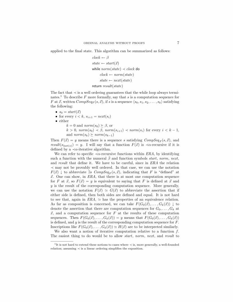
applied to the final state. This algorithm can be summarized as follows:

clock ← β

state ← start(~x)while norm(state) ≺ clock do

clock ← norm(state)state ← next(state)

return result(state)

The fact that ≺ is a well ordering guarantees that the while loop always termi-nates.1 To describe F more formally, say that s is a computation sequence forF at ~x, written CompSeqF (s, ~x), if s is a sequence 〈s0, s1, s2, . . . , sk〉 satisfyingthe following:• s0 = start(~x)• for every i < k, si+1 = next(si)• either

k = 0 and norm(s0) � β, ork > 0, norm(s0) ≺ β, norm(si+1) ≺ norm(si) for every i < k − 1,and norm(sk) � norm(sk−1)

Then F (~x) = y means there is a sequence s satisfying CompSeqF (s, ~x), andresult(slast(s)) = y. I will say that a function F (~x) is ≺α-recursive if it isdefined by a ≺α-iterative algorithm.

We can refer to specific ≺α-recursive functions within ERA, by identifyingsuch a function with the numeral β and function symbols start , norm, next ,and result that define it. We have to be careful, since in ERA the relation≺ may not be provably well ordered. In that case, we can use the notationF (~x) ↓ to abbreviate ∃s CompSeqF (s, ~x), indicating that F is “defined” at~x. One can show, in ERA, that there is at most one computation sequencefor F at ~x, so F (~x) = y is equivalent to saying that F is defined at ~x andy is the result of the corresponding computation sequence. More generally,we can use the notation F (~x) ' G(~x) to abbreviate the assertion that ifeither side is defined, then both sides are defined and equal. It is not hardto see that, again in ERA, ' has the properties of an equivalence relation.As far as composition is concerned, we can take F (G0(~x), . . . , Gk(~x)) ↓ todenote the assertion that there are computation sequences for G0, . . . , Gk at~x, and a computation sequence for F at the results of these computationsequences. Then F (G0(~x), . . . , Gk(~x)) = y means that F (G0(~x), . . . , Gk(~x))is defined, and y is the result of the corresponding computation sequence for F .Inscriptions like F (G0(~x), . . . , Gk(~x)) ' H(~x) are to be interpreted similarly.

We also want a notion of iterative computation relative to a function f .The easiest thing to do would be to allow start , norm, next , and result to

1It is not hard to extend these notions to cases where ≺ is, more generally, a well-foundedrelation; assuming ≺ is a linear ordering simplifies the exposition.

8 JEREMY AVIGAD

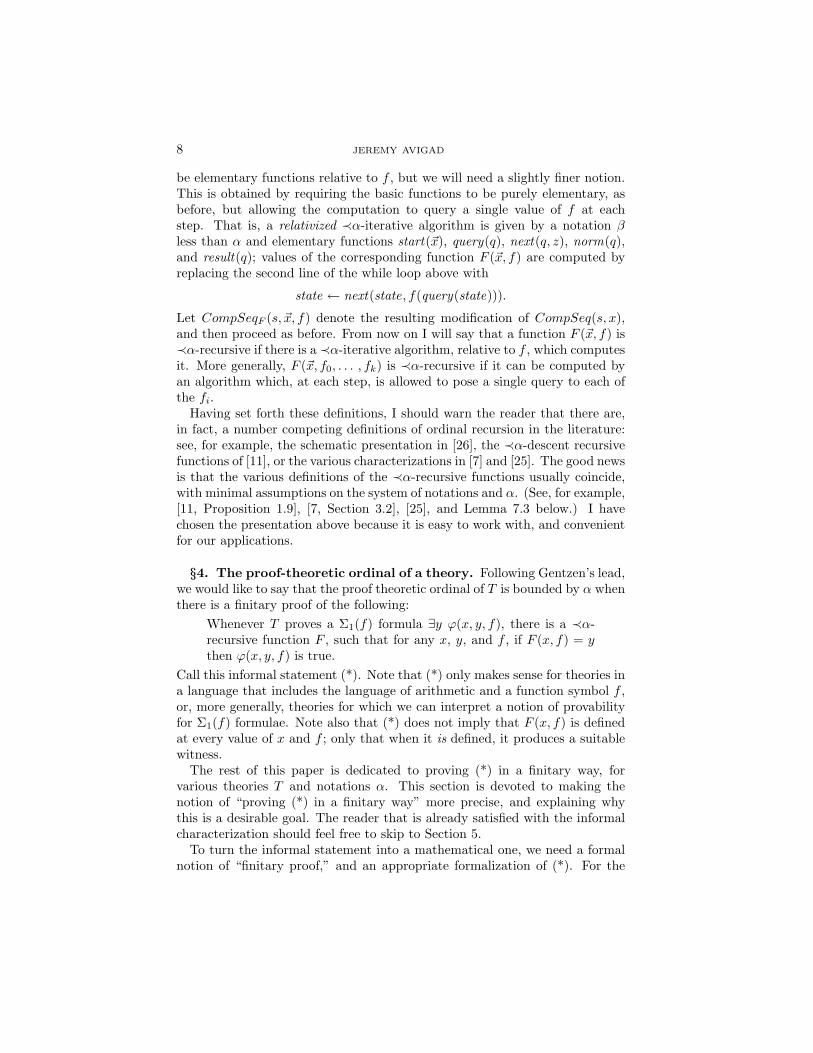
be elementary functions relative to f , but we will need a slightly finer notion.This is obtained by requiring the basic functions to be purely elementary, asbefore, but allowing the computation to query a single value of f at eachstep. That is, a relativized ≺α-iterative algorithm is given by a notation βless than α and elementary functions start(~x), query(q), next(q, z), norm(q),and result(q); values of the corresponding function F (~x, f) are computed byreplacing the second line of the while loop above with

state ← next(state, f(query(state))).

Let CompSeqF (s, ~x, f) denote the resulting modification of CompSeq(s, x),and then proceed as before. From now on I will say that a function F (~x, f) is≺α-recursive if there is a ≺α-iterative algorithm, relative to f , which computesit. More generally, F (~x, f0, . . . , fk) is ≺α-recursive if it can be computed byan algorithm which, at each step, is allowed to pose a single query to each ofthe fi.

Having set forth these definitions, I should warn the reader that there are,in fact, a number competing definitions of ordinal recursion in the literature:see, for example, the schematic presentation in [26], the ≺α-descent recursivefunctions of [11], or the various characterizations in [7] and [25]. The good newsis that the various definitions of the ≺α-recursive functions usually coincide,with minimal assumptions on the system of notations and α. (See, for example,[11, Proposition 1.9], [7, Section 3.2], [25], and Lemma 7.3 below.) I havechosen the presentation above because it is easy to work with, and convenientfor our applications.

§4. The proof-theoretic ordinal of a theory. Following Gentzen’s lead,we would like to say that the proof theoretic ordinal of T is bounded by α whenthere is a finitary proof of the following:

Whenever T proves a Σ1(f) formula ∃y ϕ(x, y, f), there is a ≺α-recursive function F , such that for any x, y, and f , if F (x, f) = ythen ϕ(x, y, f) is true.

Call this informal statement (*). Note that (*) only makes sense for theories ina language that includes the language of arithmetic and a function symbol f ,or, more generally, theories for which we can interpret a notion of provabilityfor Σ1(f) formulae. Note also that (*) does not imply that F (x, f) is definedat every value of x and f ; only that when it is defined, it produces a suitablewitness.

The rest of this paper is dedicated to proving (*) in a finitary way, forvarious theories T and notations α. This section is devoted to making thenotion of “proving (*) in a finitary way” more precise, and explaining whythis is a desirable goal. The reader that is already satisfied with the informalcharacterization should feel free to skip to Section 5.

To turn the informal statement into a mathematical one, we need a formalnotion of “finitary proof,” and an appropriate formalization of (*). For the

ORDINAL ANALYSIS WITHOUT PROOFS 9

former, let us take primitive recursive arithmetic relative to a function sym-bol f ; below we will see that weaker theories will do. In PRA(f ), we candevelop a theory of syntax, representing terms and formulae as numbers inan appropriate way; we can define the set of Σ1(f) formulas as well as namesfor the elementary functions; and we can identify ≺α-recursive functions withthe iterative algorithms that define them. In PRA(f ) we can also refer to the“value” of an elementary function at a given set of inputs, using an appropri-ate primitive recursive evaluation function for the set of elementary recursivefunctions, and we can refer to the truth value of a ∆0(f) formula at a givenset of parameters, using a truth predicate for ∆0(f) formulas that is primitiverecursive in f .

Expressed in greater detail, (*) asserts the following:For every proof d of a Σ1(f) sentence e, there is a ≺α-recursivefunction F , such that for every x, y, f , and computation sequences for F at x and f , if the result of the computation is y, then ywitnesses the truth of e at x and f .

We can get rid of the existential quantifier by requiring, more stringently, thatwe have a primitive recursive function F(d) which extracts F from the proofd; and then we can leave the universal quantification over d, e, x, y, f , ands implicit. Given a primitive recursive relation Proof T (d, e), an elementarywell ordering ≺, and a notation α, we can then take the statement “the proof-theoretic ordinal of T is at most α” to mean that there is a function symbol F ,and a PRA(f )-proof of an appropriate formalization of the following assertion:

For every d, F(d) is a ≺α-recursive function, and whenever• e is a Σ1(f) formula with free variable x,• Proof T (d, e),• CompSeqF(d)(s, x , f ), and• result(slast(s)) = y

then y witnesses the truth of e at x and f .There is, no doubt, much to criticize in this choice of a definition, but let us

consider some of the things one can say in its favor. To start with, it is strong,which is to say, it implies all the usual results of an ordinal analysis. Supposethe proof-theoretic ordinal of T is at most α, according to our definition. Thenwe have

1. A consistency proof for T2. A characterization of T ’s provably total computable functions3. A characterization of T ’s provably well-ordered computable relations

For the first, ignoring x and f and taking e to be the sentence “0 = 1,”we can conclude that the consistency of T is provable in PRA together withany principle that implies that every ≺α-iterative procedure terminates. Forthe second, we can ignore f and conclude that any Π2 statement provablein T has a ≺α-recursive Skolem function. For the third, suppose ≺′ is aΣ1-definable well ordering such that T proves ∃y (f(y + 1) 6≺′ f(y)). If the

10 JEREMY AVIGAD

order type of ≺′ is greater than α, there is an order-preserving embedding gof notations less than α into the field of ≺′. We can use the conclusion of (*)to obtain a ≺α-recursive function H(g, h), which for any h returns a value ysuch that that h(y + 1) 6≺ h(y). With minor assumptions on α, one can usethis to define a ≺α-recursive function J(g, x) that diagonalizes the functionsthat are ≺α-recursive in g, yielding a contradiction. (See [11] for additionalinformation.) Incidentally, Rathjen [24] notes that for second-order theoriesthat include arithmetic comprehension (or first-order theories that have suchconservative extensions), 3 extends to arithmetically definable orderings; andfor second-order theories that include the Σ1

1 axiom of choice, 3 extends to thehyperarithmetically definable orderings as well.

The formalization of (*) is unpalatable, and it is tempting to take the as-sertion that the proof-theoretic ordinal of T is at most α to mean that (*)is simply true. But this has the undesired consequence that adding arbitrarytrue Π1 statements to T (like consistency statements) does not increase theproof-theoretic ordinal. Similarly, defining the proof-theoretic ordinal in termsof provable well orderings means that the ordinal does not change when oneadds arbitrary true Σ1

1 sentences to the theory; see [24] for a discussion. Thispoints to a second advantage of the definition above: it is immune to theseobjections.

Our formalized version of (*) expresses a relationship between a primitiverecursive representation of T , and a system of notations for ordinals. It is wellknown that one can always cook up representations of theories and ordinalswhich render the ordinal analysis trivial, or meaningless; in this respect thedefinition above is honest, since it is really the “natural” representations thatwe care about. Some logicians are disturbed by the absence of a formal defini-tion of naturality, and so prefer to characterize the proof-theoretic ordinal asthe least upper bound to the theory’s provable well orderings; this characteri-zation is independent of the representations, but has the drawbacks mentionedabove. But the absence of such a formal definition should not concern us much.The natural representations of theories and ordinals are just those for whichthe provability of (*) is interesting; and very few mathematicians have formalcriteria which tell them which theorems of their subject have this property.2

Bounding the proof-theoretic ordinal of a theory has two aspects: proving(*), and doing so in a finitary way. In the sections that follow, I will focus onthe first; but I will proceed with the implicit understanding that once we havespecified an appropriate ordinal notation system (with properties described inthe next section), every definition, theorem, and proof can be formalized inPRA(f ). The exception is this: when I state as a theorem that “the proof-theoretic ordinal of T is at most α,” I mean simply that (*) holds, again with

2Another approach to dealing with the various definitions of “proof theoretic ordinal” inthe literature is to embrace the multiplicity, and explore the relationships between them.

See [6] for a development along these lines, as well as the discussion in [24].

ORDINAL ANALYSIS WITHOUT PROOFS 11

the implicit understanding that the formalized version of (*) can be proved inPRA(f ).

Let me close this section with two notes. First, the choice of PRA(f ) is notcrucial. We need a metatheory that is strong enough to formalize syntax andquantify over elementary functions, and is strong enough to prove Herbrand’stheorem. For these purposes, I∆0 (f ) together with the assertion that aniterated exponential function is total will suffice. If one uses a weaker classof functions in defining the ordinal-iterative algorithms, one can get by witheven weaker theories, by “pushing” the work involved in satisfying Herbrand’stheorem into the computation of the ≺α-recursive function. The possibilityof using a weaker metatheory is interesting from a foundational point of view,but it does not seem to help with the analysis of weaker theories. (For evidenceof this, see [29]. For a more fruitful approach to the analysis of weak theories,see the use of “dynamic ordinals” in [5].)

The second note has to do with lower bounds. One can take the statement“the proof-theoretic ordinal of T is exactly α” to mean that the proof-theoreticordinal of T is at most α, but it is not at most β for any β less than α. Thistakes us outside our finitary metatheory, since it requires us to show that forany such β there is no proof of the formalized version of (*) in PRA(f ). But, onthe assumption that PRA(f ) is consistent, one obtains the desired conclusionby giving a finitary proof that for every β less than α, there is a provable Σ1(f)formula that is not witnessed by any ≺β-recursive function; and one typicallyachieves this goal by developing a theory of transfinite recursion below α inT . In this paper I will focus on the upper bounds, but, in fact, all the upperbounds I provide will be sharp in this sense. (See [21, 22] for more informationon establishing the lower bounds.)

§5. Systems of ordinal notations. As noted in the last section, ordinalanalysis, as understood here, involves calibrating the strength of various the-ories relative to an elementary recursive system of ordinal notations. In thissection I will discuss the properties that our system of notations, ≺, needs tosatisfy, provably in ERA(f ). For more information on ordinal notations, see,for example, [3, 21, 22, 24].

For most of the results below, we only need to assume that ≺ is a linearordering, with elementary functions +, ·, and α 7→ ωα, for which the “usualproperties” hold. In other words, I will assume that ≺ is an elementary recur-sive ordinal notation system (ERONS) in the terminology of [11], such thatthe given functions are everywhere defined; a list of the “usual properties”they are to satisfy appears in [11, Section 1]. In particular, we will need to usethe fact that any α can be written in Cantor normal form, α = ωβ1 + . . .+ωβk

with β1 � . . . � βk. If α′ = ωβ′1 +. . .+ωβ′k′ is also in Cantor normal form, then

the symmetric sum of α and α′, written α#α′, is equal to ωγ1 + . . .+ ωγk+k′ ,where the γi’s list the βi’s and the β′i’s in decreasing order. Unlike ordinaryordinal addition, the symmetric sum is strictly monotone in both arguments.

12 JEREMY AVIGAD

Classically, ε0 is defined to be the least fixed-point of the function α 7→ ωα;equivalently, it is the limit of the sequence 〈ωn〉n∈ω, where ω0 = 1 and ωn+1 =ωωn . The statement of Theorem 9.7 assumes that there is a notation withthese properties.

More generally, the sequence of Veblen functions on any regular cardinalis defined by letting ϕ0(β) = ωβ , and otherwise letting ϕα enumerate thesimultaneous fixed points of {ϕγ | γ < α}. In Section 10, we need to assumethat there is a binary elementary function ϕ(α, β), defined on the system ofnotations, representing the Veblen functions. Writing ϕα(β) instead of ϕ(α, β),we will assume that for every α, β, γ, and δ, ϕα(β) is less than ϕγ(δ) if andonly if either• α ≺ γ and β ≺ ϕγ(δ),• α = γ and β ≺ δ, or• α � γ and ϕα(β) ≺ δ.I will say that an ordinal notation α is infinite if it is greater than or equal

to ω. Many of the lemmata and theorems below are stated most cleanly byassuming closure properties on a notation α. For reference, here are someequivalent characterizations.

Proposition 5.1. Let α be infinite. Then1. α is closed under addition if and only if it is equal to ωγ , for some γ.2. α is closed under the function β 7→ ω ·β if and only if it is equal to ωω ·γ,

for some γ.3. α is closed under multiplication if and only if it is equal to ω(ωγ), for

some γ.4. α is closed under the function β 7→ ωβ if and only if it is equal to εγ (that

is, ϕ1(γ)), for some γ.

The proof is an exercise in ordinal arithmetic (see [21]).

§6. Herbrand’s theorem. Herbrand’s theorem can be stated as follows:

Theorem 6.1. Let L be a language with at least one constant symbol, letϕ(~x) be a quantifier-free formula in L, and suppose ∃~x ϕ(~x) is provable inclassical first-order logic with equality. Then there are sequences of terms~t0, . . . ,~tk, whose free variables are among those of ∃~x ϕ(~x), such that ϕ(~t1) ∨ϕ(~t2)∨ . . .∨ϕ(~tk) is provable in propositional logic from substitution instancesof the equality axioms.

This theorem, which effectively enables us to extract additional informationfrom proofs of existential sentences, will form a cornerstone to our investiga-tions. There are model-theoretic proofs of Herbrand’s theorem: if the con-clusion fails, the set {¬ϕ(t) | t is a closed term} is propositionally consistentwith the set of all substitution instances of the equality axioms; and from asatisfying truth assignment, one can build a model of ∀x ¬ϕ(x). But Her-brand’s theorem is also an easy consequence of the cut-elimination theorem

ORDINAL ANALYSIS WITHOUT PROOFS 13

(see [8, 26]), and hence provable in our finitary metatheory. See also [27, 23]for alternative syntactic proofs, and [19] for Herbrand’s original proof.

I will say that a theory T is universal if it can be axiomatized by a universalset of sentences (or, equivalently, a quantifier-free set of formulae, since ∀~y ψ(~y)follows from an axiom ψ(~y)).

Corollary 6.2. Let L and ϕ(~x) be as above, and let T be a universal theoryin L. If T proves ∃~x ϕ(~x), then there are sequences of terms ~t0, . . . ,~tk, whosefree variables are among those of ∃~x ϕ(~x), such that T proves ϕ(~t1) ∨ ϕ(~t2) ∨. . .∨ϕ(~tk). Moreover, we can assume this formula is provable in propositionallogic from substitution instances of axioms of T and equality axioms.

Proof. Suppose T proves ∃~x ϕ(~x). Then there are (universal closures of)axioms of T , ψ1, . . . , ψk, such that ∃~x ϕ(~x) is provable from ψ1, . . . , ψk. Bythe deduction theorem, ψ1∧ . . .∧ψk → ∃~x ϕ(~x) is provable in first-order logic.Bring all the quantifiers to the front, and apply Herbrand’s theorem. a

In many cases (but not all the ones we will consider), the theory T will berich enough so that for every sequence of terms t1(~x), . . . , tk(~x) and quantifier-free formulae ϕ1(~x), . . . , ϕk−1(~x), there is a function symbol f(~x) such that Tproves

f(~x) =

t1(~x) if ϕ1(~x)t2(~x) if ¬ϕ1(~x) ∧ ϕ2(~x)...tk(~x) otherwise.

In cases like this, we can replace the sequence of terms t1, . . . , tk in the Corol-lary 6.2 with a single function symbol f .

Recall that if G(x, f) is a ≺α-recursive function, we will interpret referencesto G in the context of ERA(f ) as references to the elements β, start , norm,next , query , and result that define the iterative algorithms that computes it.As an application of Herbrand’s theorem, we have the following:

Theorem 6.3. Suppose θ(x, y, f) is a ∆0(f) formula with the free variablesshown, and suppose there is an α-recursive function G(x, f) such that ERA(f )proves G(x, f) = y → θ(x, y, f). For any x and y, if G(x, f) is defined andequal to y, then θ(x, y, f) is true.

Proof. The conclusion follows from the soundness of ERA(f ), but we haveto take care to make sure that our proof is finitary. The following proof usesan evaluation function for the set of functions that are elementary recursive inf , and a truth predicate for ∆0(f) sentences.

Suppose ERA(f ) proves G(x, f) = y → θ(x, y, f). From the definition ofG(x, f) = y, we see that it also proves CompSeqG(s, x, f)∧ result((s)last(s)) =y → θ(x, y, f). Now, suppose G(x, f) is defined and equal to y, so that in ad-dition, there is an s satisfying CompSeqG(s, x, f) and result((s)last(s)) = y.Then for this particular s, x, and y, ERA(f ) proves CompSeqG(s, x, f) ∧

14 JEREMY AVIGAD

result((s)last(s)) = y → θ(x, y, f). By Herbrand’s theorem, there is a proposi-tional proof of this fact from closed instances of equality axioms and axioms ofERA(f ). The axioms of ERA(f ) are true; so, by induction on the length of theproof, the conclusion is also true. As a result, we have that CompSeqG(s, x , f )and result(s)last(s)) = y imply θ(x, y, f). So θ(x, y, f) is true. a

This theorem seems minor, but it will play a central role. It enables us toshow that the ordinal of a theory T is less than or equal to α, by showingthat whenever T proves a statement of the form ∃y θ(x, y, f), then there is a≺α-recursive function G(x, f) which, provably in ERA(f ), finds a witness. Wewill do this repeatedly, providing explicit translations; this is what makes theaccount finitary. But we will proceed in steps, successively reducing more “ab-stract” theories to more “concrete” ones, and working “in” the target theoryas much as possible.

§7. Primitive recursion. In this section we will bound the proof-theoreticordinal of primitive recursive arithmetic. To do so, we will first show thatwith sufficient conditions on α, the ≺α-recursive functions have nice closureproperties, provably in ERA(f ). In particular, if α is ωω, we will see that onecan use a single ≺α-recursive function to assign “correct” values to a finite setof terms in PRA(f ), again provably in ERA(f ). Applying Theorem 6.3 willthen yield the desired upper bound.

The first lemma states that for α greater than 1, the ≺α-recursive functionsin f include both the purely elementary functions and f itself.

Lemma 7.1. Suppose α is greater than 0. Then for every elementary func-tion g(~x) (not involving the function f), there is a ≺α-recursive functionG(~x, f) such that ERA(f ) proves G(~x, f) ' g(~x). Also, if α is greater than 1,there is a ≺α-recursive function H(x, f) such that ERA(f ) proves H(x, f) 'f(x).

Proof. For the first claim, let the algorithm for H store ~x in the state,and then return g(~x) immediately. In other words, assuming g is arity k, takeβ = 0, start(~x) = 〈~x〉, norm(q) = 0, result(q) = g((q)0, . . . , (q)k).

For the second claim, let the algorithm for H store x in the state, query f ,and then return the result. That is, take β = 1, start(x) = x, query(q) = q,next(q, z) = z, norm(q) = 0, result(q) = q. a

The next lemma gives conditions under which the ≺α-recursive functionsare closed under composition, again provably in ERA(f ).

Lemma 7.2. Suppose α is infinite and closed under addition, and supposethat F0(~x, f), . . . , Fk(~x, f) and G(z0, . . . , zk) are ≺α-recursive functions. Thenthere is a ≺α-recursive function H(~x, f) such that ERA(f ) proves H(~x, f) 'G(F0(~x, f), . . . , Fk(~x, f)).

Proof. Let the algorithm for G carry out the algorithms for F0 throughFk on input ~x, and then send the result to the algorithm for G.

ORDINAL ANALYSIS WITHOUT PROOFS 15

In more detail, suppose the algorithm for each Fi is given by the data βi,start i, query i, next i, and result i, and suppose the algorithm for G is given byβk+1, startk+1, queryk+1, nextk+1, and resultk+1. Take the states of H to codetuples of the form 〈i, c, s, u, v〉, where i indicates the current subalgorithm, cis the setting of an ordinal “clock,” s is the state in the subalgorithm, u storesthe original input, and v stores the results which have been computed so far.The algorithm for H then corresponds to the data β, start , query , next , andresult , given as follows. First, set β = βk+1 + βk + . . .+ β0 + 1, and

start(~x) = 〈0, β0, start0(~x), ∅, 〈~x〉〉.

Assuming q is of the form 〈i, c, s, u, v〉, set

norm(q) = βk+1 + . . .+ βi + c

and

query(q) = query i(s).

Then define next(q, z) by cases, again assuming that q is of the form 〈i, c, s, u, v〉:1. If normi(s) ≺ c, we are in the middle of the computation of the ith

algorithm. In that case, set

next(q, z) = 〈i,normi(s),next i(s, z), u, v〉.

2. If normi(s) � c, we have completed the computation of the ith algorithm.(a) If i < k, store the result and begin algorithm i+ 1: set

next(q, z) = 〈i+ 1, βi+1, start i+1((u)0, . . . , (u)l), u, v 〈result i(s)〉〉,

where l is the arity of the Fi’s.(b) If i = k, begin the computation of G: set

next(q, z) = 〈k + 1, βk+1, startk+1((v)0, . . . , (v)k−1, resultk(s)), ∅, ∅〉

(c) If i = k + 1, we are done. Set next(q, z) = q to flag this fact.Finally, set result(q) = resultk+1(s).

It is not hard to show, in ERA(f ), that from a computation sequence for Hat ~x and f one can extract computation sequences for F1, . . . , Fk at ~x and f ,and a computation sequence for G at the result of those computations. a

From now on, I will rely on less formal descriptions of the algorithms, andleave the details of the implementation to the reader. The next lemma showsthat assuming that α is closed under multiplication, the set of ≺α-recursivefunctions is closed under a schema of ≺α-recursion, in which the functionsdefining the algorithm are themselves ≺α-recursive. Notice that the conditionon s in the statement of the lemma is identical to CompSeqF (s, ~x), except thatthe functions defining the algorithm is no longer assumed to be elementary.

Lemma 7.3. Suppose α is infinite and closed under multiplication. Givenβ less than α and ≺α-recursive functions Start(~x, f), Norm(q , f ), Next(q , f ),

16 JEREMY AVIGAD

and Result(q , f ), there is a ≺α-recursive function F (x, f), such that ERA(f )proves

F (~x, f) = y ↔ ∃s ((s)0 = Start(~x, f) ∧∀i < length(s) ((s)i+1 = Next((s)i, f)) ∧((length(s) = 1 ∧Norm((s)0, f) � β) ∨

(length(s) > 1 ∧Norm((s)0, f) ≺ β ∧∀i < (last(s)− 1) (Norm((s)i+1, f) ≺ Norm((s)i, f)) ∧Norm((s)last(s), f) � Norm((s)last(s)−1, f))) ∧

Result((s)last(s)) = y).

Proof. The proof is similar to the preceding one. The algorithm for Ffirst computes Start(~x, f); then iteratively computes Norm and Next , untilthe norm of the state fails to decrease; and then computes Result . Assumingthe algorithms for Start , Norm, Next , and Result are, respectively, γ-, δ-, ε-, ζ-recursive, the algorithm for H can be made η-recursive, where η =ζ + (δ + ε) · β + γ + 1. a

Using ω-recursion, we can simulate ordinary primitive recursion.

Lemma 7.4. Suppose α is infinite and closed under the function γ 7→ γ · ω.Let F0(~z, f) and F1(x,w, ~z, f) be ≺α-recursive. Then there is is a ≺α-recursivefunction G(x, ~z, f) such that ERA(f ) proves G(0, ~z, f) ' F0(~z, f) and

G(x+ 1, ~z, f) ' F1(x,G(x, ~z, f), ~z, f).

Furthermore, we can define G in such a way that ERA(f ) proves that wheneverG(x, ~z, f) is defined, there is a sequence of computation sequences 〈s0, . . . , sx〉,such that

• s0 is a computation sequence for F0 at ~z, f .• If x is greater than or equal to 1, s1 is a computation sequence for F1 at

(1, result0((s0)last(s0)), ~z), f .• For each i such that 0 < i < x, si+1 is a computation sequence for F1 at

(i, result1((si)last(si)), ~z), f .• G(x, ~z, f) = result1((sx)last(sx)).

Proof. As in the previous proof, with β = ω, we can design an algorithmthat successively computes G(0, ~z, f), G(1, ~z, f), . . . G(x, ~z, f). a

Lemmata 7.1–7.4 imply that we can assign to each function symbol g(~x, f)of PRA(f ) a ≺ωω-recursive function Fg(~x, f), in such a way that ERA(f )proves that the axioms of PRA(f ) are satisfied by these functions, at leastat arguments where they are defined. Recall that we can take the languageof PRA(f ) to include that of ERA(f ); below we will need to know that thetranslation g 7→ Fg preserves elementary functions, in the following sense.

ORDINAL ANALYSIS WITHOUT PROOFS 17

Lemma 7.5. Let g(~x, f) be an elementary function in f . Then ERA(f )proves

Fg(~x, f) ↓ → Fg(~x, f) = g(~x, f).

Proof. By induction on the definition of g, using the additional informationin Lemma 7.4. a

In fact, in ERA(f ) one can prove the existence of suitable computationsequences, and therefore show ∀~x Fg(~x, f) ↓. We will not, however, need thisfact below.

We can now show that the proof-theoretic ordinal of PRA(f ) is at most ωω.The observations following Lemma 7.4 show that one can interpret PRA(f ) inERA(f ) together the assumptions that each ≺ωω-recursive function is every-where defined. In order to use Theorem 6.3, however, we need to show thata single ≺ωω-recursive function suffices. The idea is this: we will show thatgiven any proof in PRA(f ), one can use a single ≺ωω-recursive function toassign correct values to all the terms appearing in the proof; and furthermore,that we can do this “within” ERA(f ).

Say a sequence of terms t0, . . . , tk in PRA(f ) is a formation sequence if eachti is either a constant or variable, or the result of applying a function symbolof PRA(f ) to previous terms in the sequence. To each formation sequenceS in which no variable other than x occurs, the following definition assignsa formula EvalS(e, x, f) in the language of ERA(f ), which asserts that thesequence e assigns the correct values to the members of S, when the symbolsx and f are interpreted as x and f , respectively.

Definition 7.6. For each formation sequence S in which no variable otherthan x occurs, let EvalS(e, x, f) be the formula in the language of ERA(f ),defined inductively as follows:

• Eval∅(e, x, f) is the sentence 0 = 0• If tk is the variable x, then Eval 〈t0,... ,tk〉(e, x, f) is defined to be

(e)k = x ∧ Eval 〈t0,... ,tk−1〉(e, x, f).

• If tk is of the form g(ti0 , . . . , til, f), where g is a function symbol of

PRA(f ), then Eval 〈t0,... ,tk〉(e, x, f) is

(e)k = Fg((e)i0 , . . . , (e)il, f) ∧ Eval 〈t0,... ,tk−1〉(e, x, f).

Lemma 7.7. Let S be a formation sequence of terms in the language ofPRA(f ) in which at most the variable x is free. Then there is a ≺ωω-recursivefunction G(x, f) such that ERA(f ) proves G(x, f) = e→ EvalS(e, x, f).

Proof. By induction on the length of S, using Lemmata 7.1–7.4. aGiven a proof in the quantifier-free version of PRA(f ), we can use Lemma 7.7

to find a correct evaluation of the terms appearing in the proof.

18 JEREMY AVIGAD

Lemma 7.8. Suppose PRA(f ) proves ∃y θ(x, y, f), where θ is ∆0(f). Thenthere is a ≺ωω-recursive function H(x, f) such that ERA(f ) proves H(x, f) =y → θ(x, y, f).

Proof. Suppose PRA(f ) proves ∃y θ(x, y, f). Then it also proves the for-mula ∃y (χθ(x, y, f) = 1), where χθ is a an elementary recursive characteristicfunction representing θ. By Herbrand’s theorem, there is a function symbolg(x, f) of primitive recursive arithmetic, and a proof d of χθ(x, g(x, f), f) = 1in propositional logic, from substitution instances of the equality axioms andaxioms of PRA(f ). For example, we may take d to be a sequence of quantifier-free formulae in the language of PRA(f ) such that each line either is an instanceof an axiom of PRA(f ), is an instance of an axiom of equality, is an instanceof a propositional tautology, or follows from previous lines by modus ponens(or other valid propositional inferences).

Let S be a formation sequence that includes all the terms occurring in d.Each line of d is a boolean combination of atomic formulae of the form t = s,where t and s are terms occurring in S. If ϕ is such a formula, let ϕe denotethe formula obtained by replacing each term ti by (e)i. Then by induction,one can show that for each line ϕ of d, then ERA(f ) proves

EvalS(e, x, f)→ ϕe.

When ϕ is an axiom of equality or PRA(f ), this follows from the definition ofEvalS(e, x, f); otherwise, the propositional axioms and inferences of d can bemirrored in ERA(f ).

In particular, suppose g(x, f) is the kth term in S and χθ(x, g(x, f), f) isthe lth. Since the conclusion of d is χθ(x, g(x, f), f) = 1, in ERA(f ) one canprove

EvalS(e, x, f)→ (e)l = 1.

But if e evaluates terms correctly, (e)l is equal to Fχθ(x, (e)k, f); so ERA(f )

proves

EvalS(e, x, f)→ (e)l = Fχθ(x, (e)k, f),

and hence EvalS(e, x, f) → Fχθ(x, (e)k, f) = 1. But by Lemma 7.5, ERA(f )

proves that Fχθ(x, (e)k, f) = 1 is equivalent to θ(x, (e)k, f).

In short, in ERA(f ) we can prove

EvalS(e, x, f)→ θ(x, (e)k, f).

Using Lemma 7.7, let G(x, f) be a ≺α-recursive function which returns an esatisfying EvalS(e, x, f). Using Lemmata 7.1 and 7.2 let H(x, f) be a ≺α-recursive function such that ERA(f ) proves H(x, f) ' (G(x, f))k. Puttingit all together, we have that ERA(f ) proves H(x, f) = y → θ(x, y, f), asdesired. a

By Theorem 6.3 this yields

Theorem 7.9. The proof-theoretic ordinal of PRA(f ) is at most ωω.

ORDINAL ANALYSIS WITHOUT PROOFS 19

At this point, we could extend the analysis to various forms of primitiverecursion on the ordinals, and use similar methods to obtain ordinal analysesof various extensions of PRA(f ). But instead of pursuing that, let us turninstead to theories of transfinite induction.

§8. Π1 Transfinite induction. In the last section, we saw that ordinalrecursion can be used to simulate ordinary primitive recursion; but this shouldnot have been very surprising. In this section we will be somewhat bolder: wewill augment our basic theory with function symbols that are intended todenote noncomputable functions, allowing us to prove a form of transfiniteinduction. A judicious application of Herbrand’s theorem will then enable usto extract constructive information from proofs in the augmented theory.

By Proposition 2.2, we can represent our system of notations in the languageof I∆exp

0 . If ϕ(x) is any formula in this language and β is any ordinal notation,then the principle of transfinite induction on β for ϕ is

∀γ ≺ β (∀δ ≺ γ ϕ(δ)→ ϕ(γ))→ ∀γ ≺ β ϕ(γ).

In words, this reads “if ϕ(x) is progressive on β, then it holds for every ordinalless than β.” Its contrapositive,

∃γ ≺ β ¬ϕ(γ)→ ∃γ ≺ β (¬ϕ(γ) ∧ ∀δ ≺ γ ϕ(δ))

is the least-element principle on β for ¬ϕ. If Γ is any set of formulae, thenTI (β,Γ) and LEP(β,Γ) denote, respectively, the principle of transfinite induc-tion and the least-element principle on β, restricted to formulae in Γ. Similarly,TI (≺α,Γ) and LEP(≺α,Γ) denote these principles for arbitrary β less thanα.

Our goal here is to provide ordinal analysis of the theories for the form

I∆exp0 (f ) + TI (≺α,Π1 (f )).

The following lemma gives some equivalent characterizations.

Lemma 8.1. Assume α is closed under the function β 7→ ω · β. Then overI∆exp

0 (f), the following schemata are equivalent:1. TI (≺α,Π1(f))2. LEP(≺α,Σ1(f))3. TI (≺α,∆exp

0 (f))4. LEP(≺α,∆exp

0 (f))

Proof. The contrapositive of any instance of 1 is equivalent to an instanceof 2, and vice-versa; similarly for 3 and 4. Clearly 2 implies 4, so it suffices toshow that 4 implies 2.

Let θ(γ, x) be ∆exp0 and let β be a notation less than α. Arguing in

I∆exp0 (f ) + LEP(≺α,∆exp

0 (f)), let us prove the least-element principle on βfor ∃x θ(γ, x). Let θ′(δ) be a formula which asserts that, if δ is written in theform ω · δ′ + y, then θ(δ′, y). Now suppose θ(γ, x). Then θ′(ω · γ + x). By the

20 JEREMY AVIGAD

least-element principle on ω · β for θ′, there is a least δ satisfying θ′(δ). But ifδ = ω · δ′ + y, then δ′ is the least element satisfying ∃x θ(δ′, x). a

Now let us add function symbols to ERA(f ) that enable us to interpretthe new axioms. Using the last characterization in Lemma 8.1, it is sufficientto have, for each notation β less than α and elementary relation R(~x, y, f),a function g(~x, f) which returns the least γ less than β satisfying R(~x, γ, f),whenever such a γ exists. The approach we will take is slightly more general,but not more difficult.

Given an elementary function norm(~x, z, f), let “z minimizes norm(~x, ·, f)below β” denote the following formula:

∀w (norm(~x,w, f) ≺ β → norm(~x, z, f) � norm(~z, w, f)).

In words, if anything has a norm less than β, then z has the smallest possiblenorm. Let

ERA(f ) + min(≺α, E(f))

be the theory obtained by adding, for each elementary function norm(~x, z, f)and β less than α, a new function symbol, minnorm,β(~x, f), to the language,and an axiom

“minnorm,β(~x, f) minimizes norm(~x, ·, f) below β.”

In the name of the theory, the “E(f)” indicates that the norm functions arerequired to be elementary in f ; note that that the theory does not have sym-bols, say, for elementary functions or minimization functions defined from theones we have just added.

Even for β = 1, a function minnorm,β may be nonconstructive. For example,let T (x, y, f) be an elementary relation such that ∃y T (x, y, f) is a completeΣ1(f) formula; more precisely, assume T has the property that for any Σ1(f)formula ϕ(~w, f) there is a natural number n, such that ϕ(~w, f) is equivalent,in ERA(f ), to the formula ∃y T (〈n, ~w〉, y, f). (Think of T (〈n, ~w〉, y, f) asasserting that y witnesses the truth of the Σ1(f) formula coded by n, at theparameters ~w; or T may be a version of Kleene’s T predicate, asserting thaty is a halting computation of the nth Turing machine with oracle f , on input~w. Below, we will also assume that n can be computed in an elementary wayfrom a Godel number of ϕ.) Let β = 1, and let

norm(x, z, f) ={

0 if T (x, z, f)1 otherwise.

Then minnorm,β(~x) is guaranteed to return a witness y to T (x, y, f), if thereis one; this enables us, for example, to solve the halting problem.

Lemma 8.2. For each α, ERA(f ) + min(≺α, E(f)) is a universal theorycontaining I∆exp

0 (f ) + TI (≺α,Π1 (f )).

Proof. The formula “minnorm,β(~x, f) minimizes norm(~x, ·, f) below β” isuniversal, so it suffices to show that instances of the Σ1 least-element principle

ORDINAL ANALYSIS WITHOUT PROOFS 21

are derivable from these axioms. Given a ∆exp0 formula θ(y, γ, ~x, f) with the

free variables shown and a notation β, let

norm(~x, z, f) ={

(z)1 if (z)1≺β and θ((z)0, (z)1, ~x, f)β otherwise

Arguing in ERA(f )+min(≺α, E(f)), if there is any γ satisfying ∃y θ(y, γ, ~x, f),then (minnorm,β(~x))1 is a least such one. a

We will carry out the ordinal analysis of ERA(f ) + min(≺α, E(f)) in twosteps. First, we will show that one can reduce the problem of assigning thecorrect values to a set of terms in this theory to the problem of finding avalue minimizing an appropriate norm, provably in ERA(f ). Then we willuse Herbrand’s theorem to replace the latter problem with a ≺α-recursivecalculation.

If ϕ(~x, z) is any formula in the language of ERA(f ) and β is any notation, letus say that ERA(f ) proves that ϕ(~x, y) is solvable (for y) by β-minimizationif there are elementary functions norm(~x, z, f) and result(~x, z, f) such thatERA(f ) proves

“z minimizes norm(~x, ·) below β”→ ϕ(~x, result(~x, z, f)).

Say that ERA(f ) proves that ϕ(~x, y) is solvable by≺α-minimization if it provesthat ϕ(~x, y) is solvable by β-minimization for some β less than α. Note thatthe “solution” to ϕ(~x, z) may not be unique. If ERA(f ) also proves ϕ(~x, z) ∧ϕ(~x, z′)→ z = z′ it makes sense to say that ERA(f ) proves that ϕ(~x, z) definesa function that is computable by ≺α-minimization; but for our purposes themore general notion is more useful.

The next few lemmata provide closure properties on the kinds of problemsthat are solvable by ≺α-minimization.

Lemma 8.3. For any α, if g(~x, f) is an elementary function, then ERA(f )proves that the relation g(~x, f) = y is solvable by ≺α-minimization.

Proof. Let norm(~x, z, f) be arbitrary, and let result(~x, z, f) = g(~x, f). aLemma 8.4. Suppose β is less than α, and norm(~x, y, f) is an elementary

function in f . Then ERA(f ) proves that the relation “z minimizes norm(~x, ·, f)below β” is solvable by ≺α-minimization.

Proof. Leave β and norm alone, and let result(~x, z, f) = z. aLemma 8.5. Let α be closed under addition. If ϕ0(~x, y, f), . . . , ϕk(~x, y, f)

are all solvable by ≺α-minimization, provably in ERA(f ), then so is the for-mula ϕ0(~x, (y)0, f) ∧ . . . ∧ ϕk(~x, (y)k, f).

Proof. Suppose each ϕi is solvable by βi, normi(~x, z, f), and result i(~x, z, f).We can assume without loss of generality that ERA(f ) proves that for every~x and z, normi(~x, z, f) is less than or equal to βi, by replacing normi(~x, z, f)with min(βi,normi(~x, z, f)) if necessary. Let β = β0# . . .#βk, let

norm(~x, z, f) = norm0(~x, (z)0, f)# . . .#normk(~x, (z)k, f),

22 JEREMY AVIGAD

and let

result(~x, z, f) = 〈result0(~x, (z)0, f), . . . , resultk(~x, (z)k, f)〉.

It is not hard to see that if z minimizes norm(~x, ·, f) below β, then each (z)i

minimizes normi(~x, ·, f) below βi. a

Lemma 8.6. Let α be infinite and closed under multiplication. Supposeϕ0(~x,w, f) and ϕ1(~x,w, y, f) are solvable by ≺α-minimization, for w and yrespectively, provably in ERA(f ). Then the formula

ϕ0(~x, (y)0) ∧ ϕ1(~x, (y)0, (y)1),

and the formula

∃w (ϕ0(~x,w) ∧ ϕ1(~x,w, y)),

are solvable for y by ≺α minimization, provably in ERA(f ).

Proof. Suppose ϕ0 is solved by β0, norm0(~x, z, f), and result0(~x, z, f), andϕ1 is solved by β1, norm1(~x,w, z), and result1(~x,w, f). As in the previouslemma, we can assume that norm0 and norm1 are bounded by β0 and β1

respectively. Let β = (β1 + 1)(β0 + 1) and let

norm(~x, z, f) = (β1 + 1) · norm0(~x, (z)0, f) +

norm1(~x, result0(~x, (z)0, f), (z)1).

Suppose z minimizes norm(~x, ·, f) below β. Then (z)0 minimizes norm0(~x, ·, f)below β0; otherwise we could change (z)0 and decrease the value of sum above,independent of the behavior of the second term. Fixing (z)0, we also see that(z)1 minimizes norm1(~x, result0(~x, (z)0, f), ·, f) below β1, because otherwisewe could change (z)1 and decrease the value of the sum above. To solve thefirst formula, take

result(~x, z, f) = 〈result0(~x, (z)0, f), result1(~x, result0(~x, (z)0, f), (z)1, f)〉.

To solve the second formula, take

result(~x, z, f) = result1(~x, result0(~x, (z)0, f), (z)1, f).

This completes the proof. aTaken together, the lemmata above imply that for infinite α closed under

multiplication, the functions that are computable by ≺α-minimization areclosed under composition. As an exercise, the reader can try to prove that ifF (~x, f) is a ≺α-recursive function, then it is computable by ≺α-minimization.(See also the first proof of Lemma 9.2 below.)

The next step is to show that given any formation sequence S for terms inERA(f ) + min(≺α, E(f )), the problem of finding an appropriate evaluation ofthe terms in S is solvable by ≺α-minimization. We have to be careful, since,in general, there may be more than one value that we can assign to a term ofthe form minnorm,β(t1, . . . , tk, f); so when more than one term of this form

ORDINAL ANALYSIS WITHOUT PROOFS 23

appears in the formation sequence, we have to make sure that the evaluationassigns values to these terms consistently.

Definition 8.7. For each formulation sequence S for terms in the theoryERA(f ) + min(≺α, E(f )) with no variable other than x, let EvalS(e, x, f) bethe formula in the language of ERA(f ), defined inductively as follows:• Eval∅(e, x, f) is the sentence 0 = 0• If tk is the variable x, then Eval 〈t0,... ,tk〉(e, x, f) is

(e)k = x ∧ Eval 〈t0,... ,tk−1〉(e, x, f).

• If tk is of the form g(ti0 , . . . , til, f), where g is a function symbol of

ERA(f ), then Eval 〈t0,... ,tk〉(e, x, f) is

(e)k = g((e)i0 , . . . , (e)il, f) ∧ Eval 〈t0,... ,tk−1〉(e, x, f).

• If tk is of the form minnorm,β(ti0 , . . . , til, f), let tj0 , . . . , tjm enumer-

ate all the terms before tk in S that are also of this form; and foru = 0, . . . ,m, suppose tju

is the term minnorm,β(tiu,0 , . . . , tiu,l, f). Then

Eval 〈t0,... ,tk〉(e, x, f) is the conjunction of the following:– “(e)k minimizes norm((e)i0 , . . . , (e)il

, ·, f) below β”– Eval 〈t0,... ,tk−1〉(e, x, f)–

∧mu=0((e)i0 = (e)iu,0

∧ . . . ∧ (e)il= (e)iu,l

)→ (e)k = (e)ju).

Lemma 8.8. Let α be infinite and closed under multiplication, and let S bea formation sequence of terms in the language of ERA(f ) + min(≺α, E(f )).Then ERA(f ) proves that the relation EvalS(e, x, f) is solvable for e by ≺α-minimization.

Proof. By induction on the length of S, using Lemmata 8.3–8.6. Con-sider the case where S is the sequence 〈t0, . . . , tk〉 and tk is of the formminnorm,β(ti0 , . . . , til

, f). By the induction hypothesis, ERA(f ) proves thatthe relation Eval 〈t0,... ,tk−1〉(e

′, x, f) is solvable for e′ by ≺α-minimization. ByLemma 8.4, ERA(f ) also proves that the problem of finding a value v minimiz-ing norm((e)i0 , . . . , (e)il

, ·, f) below β is solvable by ≺α-minimization. Thereis an elementary function which, given e′ and v, checks the values that e′ as-signs to previous terms in S, decides whether to assign one of these values orv to tk, and returns the resulting assignment. By Lemmata 8.3 and 8.6, thisprovides a solution to EvalS(e, x, f). a

Lemma 8.9. Let α be infinite and closed under multiplication. If θ(x, y, f)is a ∆0(f) formula such that ERA(f ) + min(≺α, E(f )) proves ∃y θ(x, y, f),then ERA(f ) proves that θ(x, y, f) is solvable for y by ≺α-minimization.

Proof. Just as in the proof of Lemma 7.8. If ERA(f ) + min(≺α, E(f ))proves ∃y θ(x, y, f), then there is a sequence of terms r0, . . . , rm and a propo-sitional proof of χθ(x, r0, f) = 1 ∨ . . . ∨ χθ(x, rm, f) = 1 from substitution in-stances of equality axioms and axioms of ERA(f ) + min(≺α, E(f )). In ERA(f ),

24 JEREMY AVIGAD

given x we can use ≺α-minimization to evaluate all the terms occurring in theproof and choose one satisfying θ. a

The key use of Herbrand’s theorem is in the proof of the following lemma.

Lemma 8.10. Suppose α is infinite and closed under multiplication, and letθ(x, y, f) be a ∆0 formula such that ERA(f ) proves θ(x, y, f) is solvable by≺α-minimization. Then there is a ≺α-recursive function F (x, f) such thatERA(f ) proves F (x, f) = y → θ(x, y, f).

Proof. The hypothesis of the lemma means that there is a β less than α,and functions norm and result , such that ERA(f ) proves

∀z (∀w (norm(x,w, f) ≺ β → norm(x, z, f) � norm(x,w, f))→θ(x, result(x, z, f), f)).

Leaving the universal quantification over z implicit, bringing the universalquantification over w to the front (where it becomes existential), and rewritingthe formula slightly, we have that ERA(f ) proves

∃w (norm(x,w, f) 6≺ β ∨ norm(x,w, f) 6≺ norm(x, z, f)→θ(x, result(x, z, f), f)).

By Herbrand’s theorem, there is a an elementary function g(x, z, f) such thatERA(f ) proves

norm(x, g(x, z, f), f) 6≺ β ∨ norm(x, g(x, z, f), f) 6≺ norm(x, z, f)→θ(x, result(x, z, f), f).

In other words, if the norm of g(x, z, f) is not less than both β and the normof z, then result(x, z, f) is the witness we are after. Our job, then, is tofind a z satisfying the antecedent of this implication. An obvious iterativealgorithm suggests itself: First set z0 = 0. If norm(x, g(x, z0, f), f) 6≺ β ornorm(x, g(x, z0, f), f) 6≺ norm(x, z0, f), we are done. Otherwise, iterativelyset zi+1 equal to g(x, zi, f), until norm(x, zi+1, f) 6≺ norm(x, zi, f). Thenresult(x, zi, f) is the value we are after.

By Lemma 7.5, norm(x, z, f) and result(x, z, f) are ≺α-recursive. The algo-rithm just described is a ≺α-iterative algorithm using ≺α-recursive functions;by Lemma 7.3, it can be carried out by a single ≺α-recursive function, provablyin ERA(f ). a

Putting the last two lemmata together yield the following

Lemma 8.11. Let α be infinite and closed under multiplication. If θ(x, y, f)is a ∆0(f) formula such that ERA(f ) + min(≺α, E(f )) proves ∃y θ(x, y, f),then there is a ≺α-recursive function F (x, f) such that ERA(f ) proves F (x, f) =y → θ(x, y, f).

Below we will need to know that Lemma 8.11 still holds with additionalfunction symbols, f0, . . . , fk. To see this, note that every proof in this section

ORDINAL ANALYSIS WITHOUT PROOFS 25

can easily be generalized in this respect; alternatively, one can take f to codea finite sequence of function symbols f0, . . . , fk, and use variant of Lemma 2.3to reduce the more general statement to that of Lemma 8.11.

Together with Theorem 6.3, Lemma 8.11 yields

Theorem 8.12. Let α be infinite and closed under multiplication. Then theproof-theoretic ordinal of I∆0 (f ) + TI (≺α,Π1 (f )) is at most α.

Since induction on the natural numbers corresponds to transfinite induc-tion on ω, and Π1 and Σ1 induction on the natural numbers are equivalent,TI (≺ωω,Π1(f)) includes IΣ1 , and we have

Theorem 8.13. The proof-theoretic ordinal of IΣ1 (f ) is at most ωω.

These bounds are sharp, and, more generally, the proof-theoretic ordinalof I∆0 (f ) + TI (≺α,Π1 (f )) is the least α′ greater than or equal to α that isclosed under multiplication.

§9. Arithmetic transfinite induction. Having dealt with Π1 transfiniteinduction, let us now extend the analysis to theories of transfinite inductionfor arbitrary arithmetic formulae. Once again, the first step is to express theseprinciples in a suitable universal theory. We will do this in a straightforwardway: we will use Skolem functions to reduce any arithmetic formula to anelementary relation, and then use minimization, as in the last section.

To start with, consider Π2 transfinite induction. Let ∃y T (x, y, f) be thecomplete Σ1(f) formula introduced in the last section, and let wit1 be a newfunction symbol with defining equation

∀y (T (x, y, f)→ T (x,wit1(x), f)).(wit1(f))

In words, if there is any y satisfying T (x, y, f), wit1 returns such a one.3 Let

ERA(f ,wit1 ) + (wit1 (f )) + min(≺α, E(f ,wit1 ))

denote the theory extending ERA(f ,wit1 ) with the defining axiom for wit1,and minimization for function symbols in the language of ERA(f ,wit1 ).

Lemma 9.1. The theory ERA(f ,wit1 ) + (wit1 (f )) + min(≺α, E(f ,wit1 )) isa universal theory containing I∆exp

0 (f ) + TI (≺α,Π2 (f )).

Proof. If ϕ(~z, f) is a Σ1(f) formula of the form ∃y θ(y, ~z, f), there isa numeral n such that ϕ(~z, f) is equivalent in ERA(f ,wit1 ) + (wit1 ) to theE(f,wit1) relation T (〈n, ~z〉,wit1(〈n, ~z〉), f). Π2(f) formulae are then equiva-lent to formulae that are Π1(f,wit1). As in the proof of Lemma 8.2, from(min(≺α, E(f ,wit1 ))) one can derive instances of transfinite induction for for-mulae of this kind. a

3We could go further to fix the interpretation of wit1 by requiring it to return the leastsuch y, if there is one, and 0 otherwise; but the additional generality will be useful in [2].

26 JEREMY AVIGAD

The following lemma enables us to bound the ordinal of the theory ofLemma 9.1.

Lemma 9.2. Let α be infinite and closed under multiplication. If θ(x, y, f)is a ∆0(f) formula such that ERA(f ,wit1 ) + (wit1 (f )) + min(≺α, E(f ,wit1 ))proves ∃y θ(x, y, f), then there is a ≺ωα-recursive function H(x, f) such thatERA(f ) proves H(x, f) = y → θ(x, y, f).

Proof. Suppose the hypothesis of the lemma holds. By the deductiontheorem, the theory ERA(f ,wit1 ) + min(≺α, E(f ,wit1 )) proves

∀u, v (T (u, v, f)→ T (u,wit1(u), f))→ ∃y θ(x, y, f).

Letting y code the pair 〈u, v〉 and rewriting yields

∃y (T ((y)0, (y)1, f) ∧ ¬T ((y)0,wit1((y)0), f)) ∨ ∃y θ(x, y, f).

Bringing the existential quantifiers to the front and combining them yields

∃y ((T ((y)0, (y)1, f)→ T ((y)0,wit1((y)0), f))→ θ(x, y, f)).

By Lemma 8.11, there is a ≺α-recursive function F such that ERA(f ,wit1 )proves

F (x, f,wit1) = y ∧ (T ((y)0, (y)1, f)→ T ((y)0,wit1((y)0), f))→ θ(x, y, f).

In words, ERA(f ,wit1 ) proves that if F (x, f,wit1) is defined, it returns eithera y showing that wit1 fails to satisfy its defining axiom at (y)0, or a y satisfyingθ(x, y, f).

The rest of the proof hinges on finding a finite interpretation of wit1 thatis robust enough to carry out the computation of F and pass the final test atthe end. Towards that goal, note that one can code a finite partial functionfrom the natural numbers to the natural numbers with a natural number. Forexample, one can take the number m to code the partial function

m(x) ={

(m)x − 1 if x ≤ last(m) and (m)x > 0undefined otherwise

Let m(x) denote the extension of m to the natural numbers, such that m(x) =0 where m is undefined. Finally, let eval(m,x) be the elementary functionwhich returns m(x). If we now take m to be a variable in the language ofERA(f ), we can interpret references to m(x) as eval(m,x). Returning tothe conclusion of the last paragraph, using Lemma 2.3 to replace wit1 byλx eval(m,x), we see that in ERA(f ) there is a proof of

F (x, f, m) = y ∧ (T ((y)0, (y)1, f)→ T ((y)0, m((y)0), f))→ θ(x, y, f).

Expanding the definition of F (x, f, m) = y, this yields a proof of

(CompSeqF (s, x, f, m) ∧ resultF ((s)last(s)) = y ∧(T ((y)0, (y)1, f)→ T ((y)0, m((y)0), f)))→ θ(x, y, f).

ORDINAL ANALYSIS WITHOUT PROOFS 27

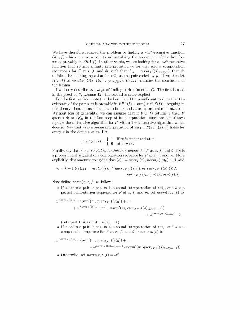
We have therefore reduced the problem to finding a ≺ωα-recursive functionG(x, f) which returns a pair 〈s,m〉 satisfying the antecedent of this last for-mula, provably in ERA(f ). In other words, we are looking for a ≺ωα-recursivefunction that returns a finite interpretation m for wit1 and a computationsequence s for F at x, f , and m, such that if y = resultF ((s)last(s)), then msatisfies the defining equation for wit1 at the pair coded by y. If we then letH(x, f) ' resultF ((G(x, f)0)last(G(x,f)0)), H(x, f) satisfies the conclusion ofthe lemma.

I will now describe two ways of finding such a function G. The first is usedin the proof of [7, Lemma 12]; the second is more explicit.

For the first method, note that by Lemma 8.11 it is sufficient to show that theexistence of the pair s,m is provable in ERA(f ) + min(≺ωα, E(f )). Arguing inthis theory, then, let us show how to find s and m using ordinal minimization.Without loss of generality, we can assume that if F (x, f) returns y then Fqueries m at (y)0 in the last step of its computation, since we can alwaysreplace the β-iterative algorithm for F with a 1 + β-iterative algorithm whichdoes so. Say that m is a sound interpretation of wit1 if T (x, m(x), f) holds forevery x in the domain of m. Let

norm ′(m,x) ={

1 if m is undefined at x0 otherwise.

Finally, say that s is a partial computation sequence for F at x, f , and m if s isa proper initial segment of a computation sequence for F at x, f , and m. Moreexplicitly, this amounts to saying that (s)0 = startF (x), normF ((s)0) ≺ β, and

∀i < k − 1 ((s)i+1 = nextF ((s)i, f(queryF,0((s)i)), m(queryF,1((s)i))) ∧normF ((s)i+1) ≺ normF ((s)i)).

Now define norm(x, z, f) as follows:• If z codes a pair 〈s,m〉, m is a sound interpretation of wit1, and s is a

partial computation sequence for F at x, f , and m, set norm(x, z, f) to

ωnormF ((s)0) · norm ′(m, queryF,1((s)0)) + . . .

+ ωnormF ((s)last(s)−1 ) · norm ′(m, queryF,1((s)last(s)−1 ))

+ ωnormF ((s)last(s)) · 2

(Interpret this as 0 if last(s) = 0.)• If z codes a pair 〈s,m〉, m is a sound interpretation of wit1, and s is a

computation sequence for F at x, f , and m, set norm(z) to

ωnormF ((s)0) · norm ′(m, queryF,1((s)0)) + . . .

+ ωnormF ((s)last(s)−1 ) · norm ′(m, queryF,1((s)last(s)−1 ))

• Otherwise, set norm(x, z, f) = ωβ .

28 JEREMY AVIGAD

Let z be a value minimizing norm(x, ·, f) below ωβ . We know that for thisz either the first or second case must hold, since taking s to be the sequence〈startF (~x)〉 and m to be the partial function that is nowhere defined satisfiesone of these two cases, and hence yields a norm less than ωβ . In fact, z must fallunder the second case: if s is a partial computation sequence, extending it byappending nextF ((s)last(s), f(query0((s)last(s))), m(query1((s)last(s)))) yields ei-ther a computation sequence or partial computation sequence with a smallernorm. Finally, let us show that if resultF ((s)last(s)) is equal to y, we haveT ((y)0, (y)1, f)→ T ((y)0, m((y)0), f). Suppose otherwise; then T ((y)0, (y)1, f)holds, but not T ((y)0, m((y)0), f). Since m is a sound interpretation of wit1,this means that (y)0 is not in the domain of m. Let i be the least value lessthan last(s) such that query1((s)i) = (y)0; there is at least one such i, since weare assuming that F queries m at this value before the end of its computation.Note that we then have norm ′(m, queryF,1((s)i)) = 1. Let m′ represent thepartial function extending m with m′((y)0) = (y)1, and let s′ be the partialcomputation sequence which is an initial segment of s of length i. Then thenorm of the pair 〈s′,m′〉 is less than the norm of the pair 〈s,m〉, contradictingthe fact that 〈s,m〉 is supposed to minimize norm(x, ·, f).

For the second proof, note that we can extract an explicit description of Gfrom the preceding argument. The iterative algorithm for G starts with thepair 〈s,m〉, where s is the sequence 〈startF (x)〉 and m is nowhere defined, andnormG is the function norm above. As long as the current state of G is apair 〈s,m〉, where s is either a partial computation sequence or a computationsequence for F at x, m, and f , and m is a sound interpretation of wit1, theargument above provides a recipe nextG for finding a pair 〈s,m〉 with a smallernorm, unless s is, in fact, a computation sequence and m satisfies the axiomfor wit1 at resultF ((s)last(s)); and in that case, resultG can just return thepair 〈s,m〉. By Lemma 7.5, T is ≺α-recursive; so startG, normG, nextG, andresultG are all ≺α-recursive functions. By Lemma 7.3, G is be ≺ωα-recursive,and the relevant properties can be proved in ERA(f ). a

Putting this all together, we have

Corollary 9.3. Let α be infinite and closed under multiplication. Thenthe proof-theoretic ordinal of I∆exp

0 (f ) + TI (≺α,Π2 (f )) is at most ωα.

More generally, let

ERA(wit1 , . . . ,witn , f ) + (witn(f )) + min(≺α, E(wit1 , . . . ,witn , f ))

denote the theory with n witnessing functions, axioms asserting that eachwit i+1 returns witnesses to a complete Σ1(wit1, . . . ,wit i, f) formula, and min-imization for functions that are elementary in wit1, . . . ,witn, f . Adapting theproof of Lemma 9.2 yields

Lemma 9.4. Let α be infinite and closed under multiplication. Supposeθ(x, y,wit1, . . . ,witn, f) is a ∆0(wit1, . . . ,witn, f) formula such that

ERA(wit1 , . . . ,witn+1 , f ) + (witn+1 (f )) + min(≺α, E(wit1 , . . . ,witn+1 , f ))

ORDINAL ANALYSIS WITHOUT PROOFS 29

proves ∃y θ(x, y,wit1, . . . ,witn, f). Then

ERA(wit1 , . . . ,witn , f ) + (witn(f )) + min(≺ωα, E(wit1 , . . . ,witn , f ))

proves it as well.

Let ωα0 = α, and ωα

n+1 = ωωαn . By induction, we have

Theorem 9.5. Let α be infinite and closed under multiplication, and let nbe greater than or equal to 0. Then the proof-theoretic ordinal of the theoryI∆exp

0 (f ) + TI (≺α,Πn+1 (f )) is at most ωαn .

In particular, for α = ωω, we have

Theorem 9.6. For n greater than or equal to 1, the proof-theoretic ordinalof IΣn(f ) is at most ωn+1.

Also, since any proof in PA(f ) is a proof in IΣn(f ), for some n, we have

Theorem 9.7. The proof-theoretic ordinal of PA(f ) is at most ε0.

More generally, let PA(f ) + TI (≺α) denote Peano arithmetic together withtransfinite induction principles for arbitrary notations β less than α and arbi-trary formulae in the language.

Theorem 9.8. Let α be infinite and closed under β 7→ ωβ. Then the proof-theoretic ordinal of PA(f ) + TI (≺α) is at most α.

In all these theorems, the bounds are sharp.

§10. Transfinite arithmetic hierarchies. In this final section, we willconsider theories with transfinite arithmetic hierarchies. We will continue touse functions as our basic second-order objects, and interpret references toa set X of natural numbers as references to its characteristic function, χX .If X is any set, the Turing jump of X, written X ′, is defined to be the set{x | ∃y T (x, y, χX)} where ∃y T (x, y, f) is the complete Σ1(f) formula fromSection 8. We can use a set X to code a sequence of such sets, by interpretingz ∈ Xy as 〈y, z〉 ∈ X. If β is an ordinal notation and 〈Hγ〉γ≺β is a sequenceof sets, then H≺β is a set which codes this sequence (with Hy = ∅ if y is thenotation for the ordinal 0, or y is not a notation less than β). Given an ordinalnotation β, a jump hierarchy on β is defined to be a set H, such that for everyγ less than β, Hγ = (H≺γ)′.

Given a notation for a limit ordinal α, we can extend the language of PAwith new symbols Hβ , for β less than α. Our goal is then to bound theproof-theoretic ordinal of theories of the form

PA(H) + H (≺α) + TI (≺α),

given by the following set of axioms: the axioms of PA, extended to the lan-guage with the new symbols; for each β less than α, an axiom asserting thatHβ is a jump hierarchy on β; and transfinite induction up to α, for arbitrary

30 JEREMY AVIGAD

formulae in new language. For an ordinal analysis, we really need to considerversions of these theories in which the induction axioms and transfinite hier-archies are relativized to a function symbol f ; but to simplify the expositionI will drop the references to f , with the implicit understanding that all thelemmata and theorems in this section are easily generalized in this way.

We can simplify the theories above in a number of ways. For one thing,in I∆exp

0 (H) one can show that if Hβ is a jump hierarchy on β, then foreach γ less than β, Hβ

≺γ is a transfinite hierarchy on γ. This means thatfor any particular proof of an arithmetic statement, it suffices to use only asingle new symbol Hβ , for a sufficiently large β less than α. Also, if ϕ(Hβ)is an arithmetic formula relative to one of these hierarchies, there is a naturalnumber n such that I∆exp

0 (H) proves that ϕ(Hβ) is equivalent to a formulathat is ∆0(Hβ+n). This means that nothing is lost of we restrict the transfiniteinduction principles to formulae that are ∆0 in the new symbols. Finally, sincethe transfinite induction axioms include ordinary induction, one can replacePA(H) by I∆exp

0 (H).In carrying out the ordinal analysis we will need to make use of Kleene’s

recursion theorem. Let R0, R1, R2, . . . denote a standard enumeration of thepartial computable functions (of various arities). The recursion theorem saysthat for any partial computable function f(x, e), there is an index e for a unarypartial computable function Re, satisfying Re(x) ' f(e, x) for every e and x.Since there is a universal partial computable function, this allows us to define apartial computable function Re in terms of itself, and its own index. A theoryof computable functions strong enough to prove the recursion theorem canbe developed in ERA or I∆exp

0 , interpreting references to such functions byreferences to their indices. If I say that a function f is “computable” insteadof “partial computable,” I mean, implicitly, that f is total.

Once again, the first step in our ordinal analysis is to embed the theorieswe are interested in appropriate universal theories. An obvious strategy is toextend the Σn witness functions of the previous section to transfinite ones.We can take a single function f to represent a sequence of functions fx, wherefx(y) = f(〈x, y〉); and given a function f and a notation γ, we can take f �γ

to denote the function

f �γ (z) ={f(z) if (z)0 ≺ γ0 otherwise

Then a transfinite witness function wit on β satisfies the following:

∀γ ≺ β ∀x, y (T (x, y,wit �γ)→ T (x,witγ(x),wit �γ)).

Now, for each β less than α, we can add a function symbol witβ , to denote awitness function on β. Then

ERA(W) + wit(≺α) + min(≺α, E(W))

denotes the theory that extends elementary computable arithmetic (relativeto the new function symbols) with axioms that assert that the new symbols

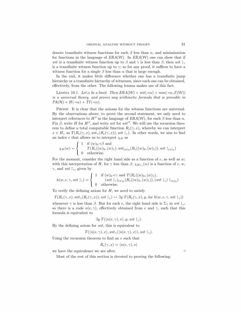
ORDINAL ANALYSIS WITHOUT PROOFS 31

denote transfinite witness functions for each β less than α, and minimizationfor functions in the language of ERA(W). In ERA(W) one can show that ifwit is a transfinite witness function up to β and γ is less than β, then wit �γ

is a transfinite witness function up to γ; so for any proof, it suffices to have awitness function for a single β less than α that is large enough.

In the end, it makes little difference whether one has a transfinite jumphierarchy or a transfinite hierarchy of witnesses, since each one can be obtained,effectively, from the other. The following lemma makes use of this fact.

Lemma 10.1. Let α be a limit. Then ERA(W) + wit(≺α) + min(≺α, E(W))is a universal theory, and proves any arithmetic formula that is provable inPA(H) + H (≺α) + TI (≺α).

Proof. It is clear that the axioms for the witness functions are universal.By the observations above, to prove the second statement, we only need tointerpret references to Hβ in the language of ERA(W), for each β less than α.Fix β, write H for Hβ , and write wit for witβ . We will use the recursion theo-rem to define a total computable function Re(γ, x), whereby we can interpretx ∈ Hγ as T (Re(γ, x),witγ(Re(γ, x)),wit �γ). In other words, we aim to findan index e that allows us to interpret χH as

χH(w) =

1 if (w)0≺β andT (Re((w)0, (w)1),wit (w)0(Re((w)0, (w)1)),wit �(w)0)

0 otherwise.

For the moment, consider the right hand side as a function of e, as well as w;with this interpretation of H, for γ less than β, χH�γ (w) is a function of e, w,γ, and wit �γ , given by

h(w, e, γ,wit �γ) =

1 if (w)0≺γ and T (Re((w)0, (w)1),(wit �γ)(w)0(Re((w)0, (w)1)), (wit �γ) �(w)0)

0 otherwise.

To verify the defining axiom for H, we need to satisfy

T (Re(γ, x),witγ(Re(γ, x)),wit �γ)↔ ∃y T (Re(γ, x), y, λw h(w, e, γ,wit �γ))

whenever γ is less than β. But for each e, the right hand side is Σ1 in wit �γ ;so there is a code n(e, γ), effectively obtained from e and γ, such that thisformula is equivalent to

∃y T (〈n(e, γ), x〉, y,wit �γ).

By the defining axiom for wit , this is equivalent to

T (〈n(e, γ), x〉,witγ(〈n(e, γ), x〉),wit �γ).

Using the recursion theorem to find an e such that

Re(γ, x) = 〈n(e, γ), x〉we have the equivalence we are after. a

Most of the rest of this section is devoted to proving the following:

32 JEREMY AVIGAD

Lemma 10.2. Let α be infinite and closed under multiplication. If θ(x, y)is a ∆0 formula and ERA(W) + wit(≺α) + min(≺α, E(W)) proves ∃y θ(x, y),then PA + TI (≺ϕα(0 )) proves it as well.

From now on, fix α, and let us work in PA + TI (≺ϕα(0 )). In this theory wecan refer to computable functions by identifying them with their indices, andwe can refer to ∆0 formulae by identifying them with their Godel numbers. Thedefinitions which follow should be seen as taking place in PA + TI (≺ϕα(0 )),with these conventions.

In the last section, we saw, roughly speaking, that given a ≺η-computablefunction that queries wit1, and, with “adequate” responses, finds a witnessto a Σ1 formula, we can effectively obtain a ≺ωη-computable function thatfinds a witness outright. In the current setting, this will let us transform a≺η-iterative computation that queries a witness hierarchy on µ+1, to a ≺ωη-iterative computation which queries a witness hierarchy on µ. To extend thisreduction to the transfinite, we need to generalize the notion of an iterativecomputation.

A ≺η-computable (rather than recursive) functional F (f) is given by a no-tation µF≺η, a value startF , and computable (rather than elementary) func-tions normF (q), nextF (q, z), queryF (q), and resultF (q). Given f , the notionsCompSeqF (s, f), F (f) ↓, F (f) = y, and so on, are defined as in Section 3.

Using sequences, we can express the assertion that f is a witness hierarchyup to µ with a formula ∀y W (y, µ, f), where W (y, µ, f) is given by

(y)0 ≺ µ ∧ T ((y)1, (y)2, f �(y)0)→ T ((y)1, f((y)1), f �(y)0).

Think ofW (y, µ, f) as asserting that f looks like a transfinite witness hierarchyon µ, “locally,” at y. Let θ(y, f) be (the code of) a formula that is ∆0(f), letη, µ, and γ be notations with γ less than µ, and let F (f) be a ≺η-computablefunction. By way of notation, take

F `ηµ ∃y θ(y,witγ)

to mean

∀m, y (F (m) = y ∧W (y, µ, m)→ Tr∆0(pθ(y, m �γ)q)),

where Tr∆0 is a truth predicate for ∆0 formulae. In words, F `ηµ ∃y θ(y,witγ)

means that if F (m) is equal to y and, at y, m looks like a witness hierarchy onµ at y, then θ(y, m �γ) is true. Take `η

µ ∃y θ(y,witγ) to assert the existenceof such an F .

(Stepping outside PA + TI (≺ϕα(0 )) for a moment, we can say that `ηµ

∃y θ(y,witγ) implies that ∃y θ(y,witγ) holds for any transfinite witness func-tion witγ . Reason as follows: given F satisfying `η

µ ∃y θ(y,witγ) and a trans-finite witness function witγ , let witµ be a transfinite witness function withwitµ �γ= witγ , and letm be a finite partial function agreeing with witµ, definedat enough values to carry out the computation of F , satisfy Wµ at the result

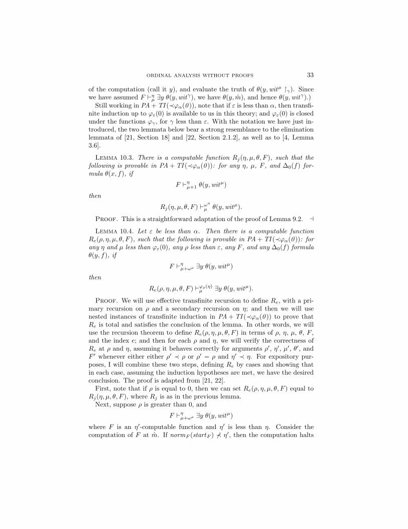
ORDINAL ANALYSIS WITHOUT PROOFS 33

of the computation (call it y), and evaluate the truth of θ(y,witµ �γ). Sincewe have assumed F `η

µ ∃y θ(y,witγ), we have θ(y, m), and hence θ(y,witγ).)Still working in PA + TI (≺ϕα(0 )), note that if ε is less than α, then transfi-

nite induction up to ϕε(0) is available to us in this theory; and ϕε(0) is closedunder the functions ϕγ , for γ less than ε. With the notation we have just in-troduced, the two lemmata below bear a strong resemblance to the eliminationlemmata of [21, Section 18] and [22, Section 2.1.2], as well as to [4, Lemma3.6].

Lemma 10.3. There is a computable function Rj(η, µ, θ, F ), such that thefollowing is provable in PA + TI (≺ϕα(0 )): for any η, µ, F , and ∆0(f) for-mula θ(x, f), if

F `ηµ+1 θ(y,witµ)

then

Rj(η, µ, θ, F ) `ωη

µ θ(y,witµ).

Proof. This is a straightforward adaptation of the proof of Lemma 9.2. a

Lemma 10.4. Let ε be less than α. Then there is a computable functionRe(ρ, η, µ, θ, F ), such that the following is provable in PA + TI (≺ϕα(0 )): forany η and µ less than ϕε(0), any ρ less than ε, any F , and any ∆0(f) formulaθ(y, f), if

F `ηµ+ωρ ∃y θ(y,witµ)

then

Re(ρ, η, µ, θ, F ) `ϕρ(η)µ ∃y θ(y,witµ).

Proof. We will use effective transfinite recursion to define Re, with a pri-mary recursion on ρ and a secondary recursion on η; and then we will usenested instances of transfinite induction in PA + TI (≺ϕα(0 )) to prove thatRe is total and satisfies the conclusion of the lemma. In other words, we willuse the recursion theorem to define Re(ρ, η, µ, θ, F ) in terms of ρ, η, µ, θ, F ,and the index e; and then for each ρ and η, we will verify the correctness ofRe at ρ and η, assuming it behaves correctly for arguments ρ′, η′, µ′, θ′, andF ′ whenever either either ρ′ ≺ ρ or ρ′ = ρ and η′ ≺ η. For expository pur-poses, I will combine these two steps, defining Re by cases and showing thatin each case, assuming the induction hypotheses are met, we have the desiredconclusion. The proof is adapted from [21, 22].

First, note that if ρ is equal to 0, then we can set Re(ρ, η, µ, θ, F ) equal toRj(η, µ, θ, F ), where Rj is as in the previous lemma.

Next, suppose ρ is greater than 0, and

F `ηµ+ωρ ∃y θ(y,witµ)

where F is an η′-computable function and η′ is less than η. Consider thecomputation of F at m. If normF (startF ) 6≺ η′, then the computation halts

34 JEREMY AVIGAD

immediately. In that case, set y = resultF (startF ); then we have

W (y, µ+ ωρ, m)→ θ(y, m �µ).

But for this particular y, W (y, µ+ ωρ, m) only depends on values of m whosefirst component is at most (y)0, assuming (y)0 ≺ µ + ωρ; so there is a ρ′ ≺ ρ

and n such that W (µ+ωρ, y, m) holds if and only if W (µ+ωρ′ ·n, y, m) does.In other words, for this F , we have

F `η

µ+ωρ′ ·n ∃y θ(y,witµ).

Applying, successively,

Re(ρ′, η, µ, θ, ·), Re(ρ′, ϕρ′(η), µ, θ, ·), . . . , Re(ρ′, ϕn−1ρ′ (η), µ, θ, ·)

yields a G satisfying

G `ϕn

ρ′ (η)µ ∃y θ(y,witµ).

Since η � ϕρ(η) and ρ′ ≺ ρ we have ϕnρ′(η) � ϕρ(η), so

G `ϕρ(η)µ ∃y θ(y,witµ).

as required.Finally, consider the case where normF (startF ) ≺ η′. Consider the next step

in the computation of F : if the first state, q0, is startF , and queryF (startF )is equal to k, then the second state, q1, is nextF (startF , m(k)). If (k)0 isless than µ + ωρ, let n and ρ′ be such that (k)0 is less than µ + ωρ′·n. (If(k)0 is not less than µ + ωρ, then the value of m(k) is irrelevant, and we cantake n and ρ′ to be 0 in the argument which follows.) For each l, let Gl bethe η′-computable function which continues the computation of F , assumingthat m(k) returns l; in other words, startGl

is equal to nextF (startF , l), whilenormGl

, nextGl, queryGl

, and resultGlare just normF , nextF , queryF , and

resultF , respectively. Then it is not hard to see that for each l,

Gl `η′

µ+ωρ ∃y (witµ+ωρ′ ·n(k) = l→ θ(y,witµ+ωρ′ ·n �µ)).

After all, for any number m, if s is a computation sequence for Gl at m,resultGl

((s)last(s))) = y, W (y, µ + ωρ, m), and m �µ+ωρ′ ·n (k) = l, thenprepending startF to s yields a computation sequence for F at m return-ing the same result; and since F `η

µ+ωρ θ(y,witµ), we have θ(y, m �µ). Now,note that µ+ ωρ is equal to (µ+ ωρ′ · n) + ωρ, since, in general, α+ ωβ = ωβ

whenever α ≺ ωβ . For each l, let θl be the formula

f(k) = l→ θ(y, f �µ)

and let

Gl = Re(ρ, η′, µ+ ωρ′ · n, θl, Gl).

By the inductive hypothesis we have that for each l,

Gl `ϕρ(η′)

µ+ωρ′ ·n ∃y (witµ+ωρ′ ·n(k) = l→ θ(y,witµ+ωρ′ ·n �µ)).

ORDINAL ANALYSIS WITHOUT PROOFS 35

Let G′(f) be the ϕρ(η′)-computable function which, in the first step, evaluatesf at k; and if the result is l, continues with Gl. Then we have

G′ `ϕρ(η′)+1

µ+ωρ′ ·n ∃y θ(y,witµ),

since if s is a computation sequence for G′ at m and l = m(k), then droppingthe first element of s yields a computation sequence for Gl at m with the sameresult. Finally, applying Re n times with first argument ρ′, we obtain a Gsatisfying

G `ϕn

ρ′ (ϕρ(η′)+1)µ ∃y θ(y,witµ).

Since ϕnρ′(ϕρ(η′) + 1) is less than ϕρ(η), we have G `ϕρ(η)

µ ∃y θ(y,witµ), asdesired.

To justify the use of the recursion theorem, we only need to verify that ineach of the three paragraphs above, G was obtained effectively from η, µ, ρ, θ,F , and the index e. This is straightforward. Then, using transfinite inductionup to ε on ρ, with a secondary transfinite induction up to ϕε(0) on η, we needto verify in PA + TI (≺ϕα(0 )) that for every ρ, η, µ, θ, and F , Re is defined,and if F satisfies the hypothesis of the lemma, then Re returns a G witnessingthe conclusion. But this is the argument we have just sketched. a

Proof of Lemma 10.2. Suppose the theory PA(H) + H(≺α) + TI(≺α)proves ∃y θ(x, y). By Lemma 10.1, we have that ∃y θ(x, y) is also provablein ERA(W) + wit(≺α) + min(≺α). By the observations above, ∃y θ(x, y) istherefore provable in the theory ERA(witα′) + ∀y W (y , α′,witα′) + min(≺α),for an α′ less than α that is large enough. By the deduction theorem andLemma 8.11, there is a ≺α-recursive function F such that ERA(witα′) proves

F (x,witα′) = y ∧W (y, α′,witα′)→ θ(x, y).

Suppose F is α′′-recursive, where α′′ is less than α. Pick ε large enough sothat we have α′, α′′ ≺ ε ≺ α.

Now argue in PA + TI (≺ϕα(0 )). For each x, let Fx(f) be α′′-computablefunctional which, for each f , returns F (x, f). Since ERA(f ) is sound, Fx

satisfies

Fx `α′′+1α′+1 ∃y θ(x, y).

Using Lemma 10.4 , we have that for each x there is a function Gx(f) satisfying

Gx `ϕα′+1(α

′′+1)

0 ∃y θ(x, y).

In other words, for any m, if Gx(m) is defined then it returns a value y satis-fying θ(x, y) outright. Let m be the partial function that is nowhere defined;using transfinite induction up to ϕα′+1(α′′ + 1) we can show that Gx(m) isdefined, and so ∃y θ(x, y) is true. a

Relativizing this theorem to an additional function symbol f , we have

36 JEREMY AVIGAD

Theorem 10.5. Let α be infinite and closed under multiplication. Then theproof-theoretic ordinal of PA(H, f ) + H (≺α) + TI (≺α) is at most ϕ(≺α, 0).

If Γ0 is the least fixed point of the function α 7→ ϕ(α, 0), we have thefollowing:

Theorem 10.6. PA(H, f ) + H (≺Γ0 ) + TI (≺Γ0 ) has proof-theoretic ordi-nal at most Γ0.

Also, relativizing the proof of Theorem 10.5 to finite witness functions, andthen interpreting references to these witness functions in PA(f ), yields

Theorem 10.7. Let α be infinite and closed under multiplication. Then anyformula that is arithmetic in f and provable in PA(H, f ) + H (≺α) + TI (≺α)is also provable in PA(f ) + TI (≺ϕα(0 )).

REFERENCES

[1] Wilhelm Ackermann, Zur Widerspruchsfreiheit der Zahlentheorie, MathematischeAnnalen, vol. 93 (1940), pp. 1–36.

[2] Jeremy Avigad, An ordinal analysis of admissible set theory using recursion onordinal notations, submitted.

[3] Jeremy Avigad and Richard Sommer, A model-theoretic approach to ordinal anal-

ysis, The Bulletin of Symbolic Logic, vol. 3 (1997), pp. 17–52.[4] , The model-theoretic ordinal analysis of predicative theories, The Journal of

Symbolic Logic, vol. 64 (1999), pp. 327–349.[5] Arnold Beckmann, Separating fragments of bounded arithmetic, Ph.D. thesis,

Westfalische Wilhelms-Universitat, Munster, 1996.

[6] Lev Beklemishev, Proof-theoretic analysis by iterated reflection, Institute forMathematical Logic, University of Munster, preprint, 1999. http://wwwmath.uni-muenster.de/inst/logik/publ/pre/6.html.

[7] Samuel Buss, The witness function method and provably recursive functions of Peanoarithmetic, Proceedings of the ninth international congress on logic, methodology, andphilosophy of science, Uppsala, Sweden, 1991 (D. Westerstahl D. Prawitz, B. Skyrms,editor), Elsevier North-Holland, Amsterdam, 1994, pp. 29–68.

[8] , First-order proof theory of arithmetic, in Buss [9].

[9] Samuel Buss (editor), The handbook of proof theory, North-Holland, Amsterdam,1998.

[10] Timothy Carlson, Ranked partial structures, preprint.

[11] Harvey Friedman and Michael Sheard, Elementary descent recursion and prooftheory, Annals of Pure and Applied Logic, vol. 71 (1995), pp. 1–45.

[12] Harvey Friedman, Iterated inductive definitions and Σ12−AC, Intuitionism and

proof theory (A. Kino, J. Myhill, and R. E. Vesley, editors), North-Holland, Amsterdam,1970, pp. 435–442.

[13] Harvey Friedman, Kenneth McAloon, and Stephen Simpson, A finite combi-

natorial principle which is equivalent to the 1-consistency of predicative analysis, PatrasLogic Symposion (G. Metakides, editor), North-Holland, Amsterdam, 1982, pp. 197–230.

[14] Gerhard Gentzen, Untersuchungen uber das logische Schliessen, MathematischeZeitschrift, vol. 39 (1935), pp. 176–210, 405–431, translated as “Investigations into LogicalDeduction” in [16], pages 68–131.

ORDINAL ANALYSIS WITHOUT PROOFS 37

[15] , Neue Fassung des Widerspruchsfreiheit fur die reine Zahlentheorie,

Forschungen zur Logik und zur Grundlegung der exakten Wissenschaften, New Series

4 (1938), pp. 19–44, translated as “New Version of the Consistency Proof for ElementaryNumber Theory” in [16], pages 252–286.

[16] , Collected works, North-Holland, Amsterdam, 1969, Edited by M. E. Szabo.

[17] Petr Hajek and Pavel Pudlak, Metamathematics of first-order arithmetic,Springer, Berlin, 1993.

[18] Jacques Herbrand, Recherches sur la theorie de la demonstration, Ph.D. thesis,University of Paris, 1930, English translation in [19].

[19] , Collected works, Harvard University Press, Cambridge, 1971, Warren Gold-

farb, editor.

[20] Grigori Mints and Sergei Tupailo, Epsilon subsitution method for the rami-fied language and ∆1

1-comprehension rule, Logic and foundations of mathematics (An-

drea Cantini et al., editor), Kluwer, the Netherlands, 1999, pp. 107–130.[21] Wolfram Pohlers, Proof theory: An introduction, Lecture Notes in Mathematics

#1407, Springer, Berlin, 1989.

[22] , Subsystems of set theory and second order number theory, in Buss [9].[23] Joseph Quinsey, Some problems in logic, Ph.D. thesis, Oxford University, 1980.[24] Michael Rathjen, The realm of ordinal analysis, Sets and proofs (Leeds, 1997),

Cambridge Univ. Press, Cambridge, 1999, pp. 219–279.[25] H. E. Rose, Subrecursion: Functions and hierarchies, Clarendon Press, Oxford,

1984.

[26] Helmut Schwichtenberg, Proof theory: Some aspects of cut-elimination, in Thehandbook of mathematical logic (Jon Barwise, editor), North-Holland, Amsterdam, 1977,pp. 867–895.

[27] Joseph Shoenfield, Mathematical logic, Addison Wesley, Reading, Massachusetts,1967.

[28] Richard Sommer, Transfinite induction and hierarchies generated by transfiniterecursion within Peano arithmetic, Ph.D. thesis, University of California, Berkeley, 1990.

[29] , Ordinal arithmetic in I∆0, Arithmetic, proof theory, and computational

complexity (Peter Clote and Jan Krajicek, editors), Oxford University Press, Oxford, 1993,pp. 320–363.

[30] Alex Wilkie and Jeff Paris, On the scheme of induction for bounded arithmetic

formulas, Annals of Pure and Applied Logic, vol. 35 (1987), pp. 261–302.

E-mail : avigad@cmu.eduURL: http://www.andrew.cmu.edu/∼avigad

DEPARTMENT OF PHILOSOPHY, CARNEGIE MELLON UNIVERSITY, PITTSBURGH,

PA 15213, USA