Embed Size (px)
Citation preview

Parallel, Adaptive Scientific Computation in Heterogeneous,Hierarchical, and Non-Dedicated Computing Environments
Jim Teresco
Department of Computer ScienceWilliams CollegeWilliamstown, Massachusetts
National Institute of Standards and TechnologyMathematical & Computational Sciences Division Seminar Series
June 15, 2006
Yet another Powerpoint-free presentation!
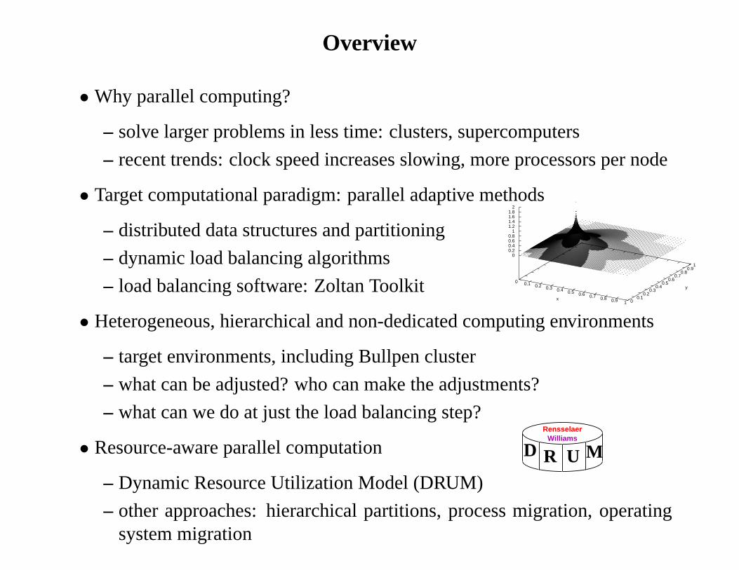
Overview
• Why parallel computing?
– solve larger problems in less time: clusters, supercomputers
– recent trends: clock speed increases slowing, more processors per node
• Target computational paradigm: parallel adaptive methods
– distributed data structures and partitioning
– dynamic load balancing algorithms
– load balancing software: Zoltan Toolkit
• Heterogeneous, hierarchical and non-dedicated computingenvironments
– target environments, including Bullpen cluster
– what can be adjusted? who can make the adjustments?
– what can we do at just the load balancing step?
• Resource-aware parallel computation
– Dynamic Resource Utilization Model (DRUM)
– other approaches: hierarchical partitions, process migration, operatingsystem migration
0 0.1 0.2 0.3 0.4 0.5 0.6 0.7 0.8 0.9 1x 0
0.10.2
0.30.4
0.50.6
0.70.8
0.91
y
00.20.40.60.8
11.21.41.61.8
2
MRensselaer
Williams
D R U
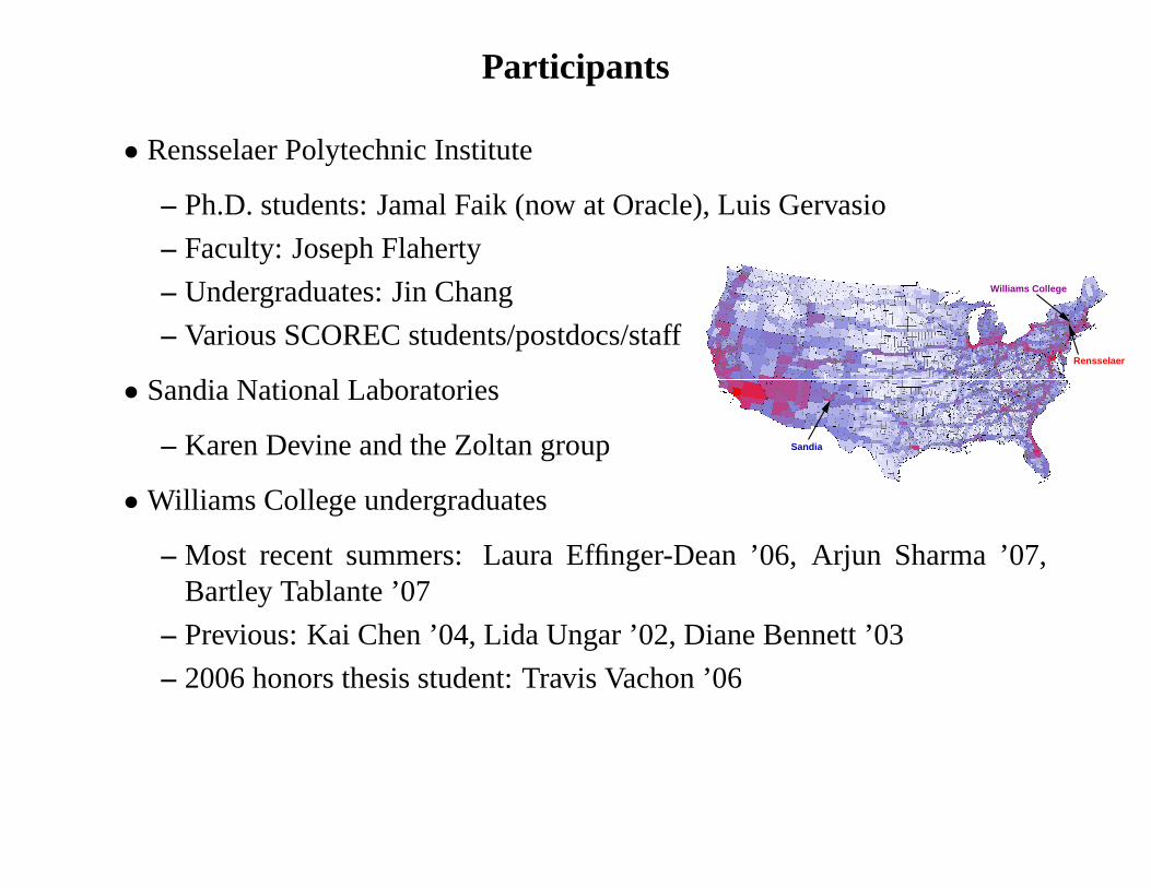
Participants
• Rensselaer Polytechnic Institute
– Ph.D. students: Jamal Faik (now at Oracle), Luis Gervasio
– Faculty: Joseph Flaherty
– Undergraduates: Jin Chang
– Various SCOREC students/postdocs/staff
• Sandia National Laboratories
– Karen Devine and the Zoltan group
• Williams College undergraduates
– Most recent summers: Laura Effinger-Dean ’06, Arjun Sharma ’07,Bartley Tablante ’07
– Previous: Kai Chen ’04, Lida Ungar ’02, Diane Bennett ’03
– 2006 honors thesis student: Travis Vachon ’06
Williams College
Sandia
Rensselaer
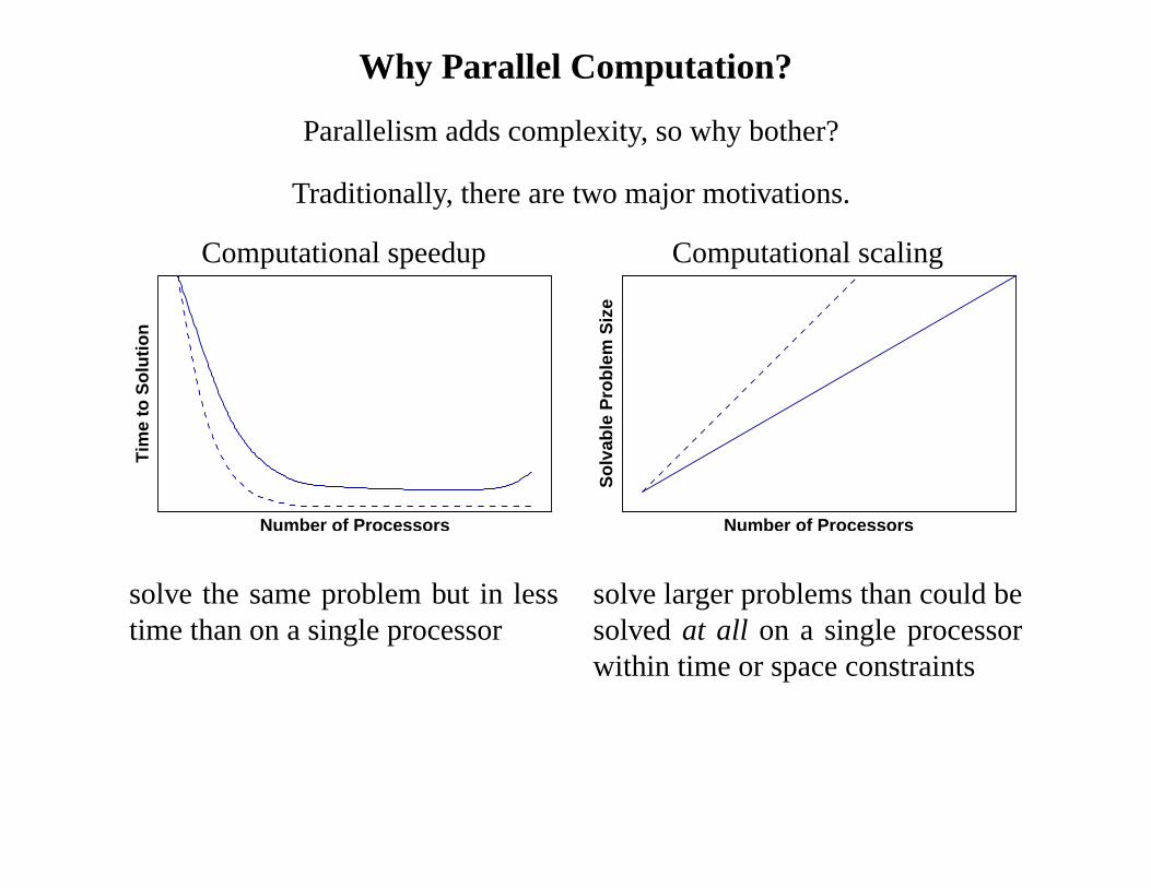
Why Parallel Computation?
Parallelism adds complexity, so why bother?
Traditionally, there are two major motivations.
Computational speedup Computational scaling
Number of Processors
Tim
e to
So
luti
on
Number of Processors
So
lvab
le P
rob
lem
Siz
esolve the same problem but in lesstime than on a single processor
solve larger problems than could besolvedat all on a single processorwithin time or space constraints
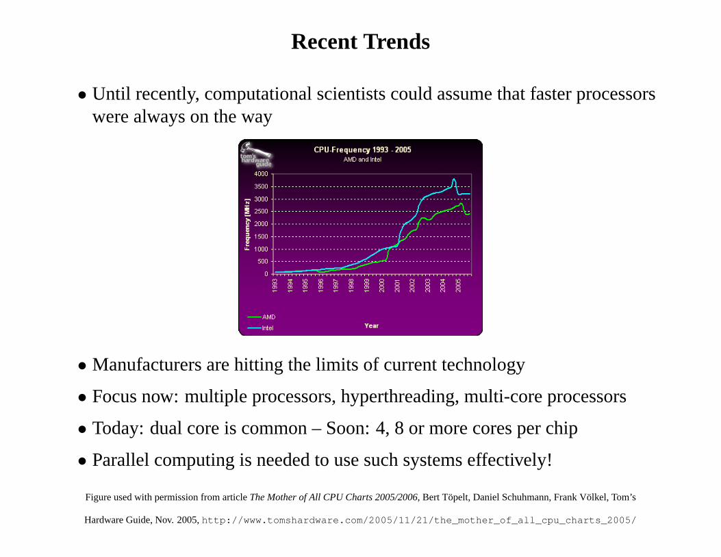
Recent Trends
• Until recently, computational scientists could assume that faster processorswere always on the way
• Manufacturers are hitting the limits of current technology
• Focus now: multiple processors, hyperthreading, multi-core processors
• Today: dual core is common – Soon: 4, 8 or more cores per chip
• Parallel computing is needed to use such systems effectively!
Figure used with permission from articleThe Mother of All CPU Charts 2005/2006, Bert Topelt, Daniel Schuhmann, Frank Volkel, Tom’s
Hardware Guide, Nov. 2005,http://www.tomshardware.com/2005/11/21/the_mother_of_all_cpu_charts_2005/
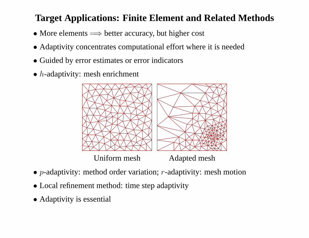
Target Applications: Finite Element and Related Methods
• More elements=⇒ better accuracy, but higher cost
• Adaptivity concentrates computational effort where it is needed
• Guided by error estimates or error indicators
• h-adaptivity: mesh enrichment
Uniform mesh Adapted mesh
• p-adaptivity: method order variation;r-adaptivity: mesh motion
• Local refinement method: time step adaptivity
• Adaptivity is essential
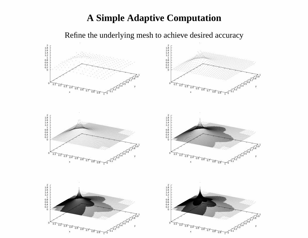
A Simple Adaptive Computation
Refine the underlying mesh to achieve desired accuracy
0 0.1 0.2 0.3 0.4 0.5 0.6 0.7 0.8 0.9 1x 0
0.10.2
0.30.4
0.50.6
0.70.8
0.91
y
00.20.40.60.8
11.21.41.61.8
2
0 0.1 0.2 0.3 0.4 0.5 0.6 0.7 0.8 0.9 1x 0
0.10.2
0.30.4
0.50.6
0.70.8
0.91
y
00.20.40.60.8
11.21.41.61.8
2
0 0.1 0.2 0.3 0.4 0.5 0.6 0.7 0.8 0.9 1x 0
0.10.2
0.30.4
0.50.6
0.70.8
0.91
y
00.20.40.60.8
11.21.41.61.8
2
0 0.1 0.2 0.3 0.4 0.5 0.6 0.7 0.8 0.9 1x 0
0.10.2
0.30.4
0.50.6
0.70.8
0.91
y
00.20.40.60.8
11.21.41.61.8
2
0 0.1 0.2 0.3 0.4 0.5 0.6 0.7 0.8 0.9 1x 0
0.10.2
0.30.4
0.50.6
0.70.8
0.91
y
00.20.40.60.8
11.21.41.61.8
2
0 0.1 0.2 0.3 0.4 0.5 0.6 0.7 0.8 0.9 1x 0
0.10.2
0.30.4
0.50.6
0.70.8
0.91
y
00.20.40.60.8
11.21.41.61.8
2

Parallel Strategy
• Dominant paradigm: Single Program Multiple Data (SPMD)
– distributed memory; communication via message passing (usually MPI)
• Can run the same software on shared and distributed memory systems
• Adaptive methods lend themselves to linked structures
– automatic parallelization is difficult
• Must explicitly distribute the computation via a domain decomposition
Subdomain 4
Subdomain 3Subdomain 1
Subdomain 2
• Distributed structures complicate matters
– interprocess links, boundary structures, migration support
– very interesting issues, but not today’s focus
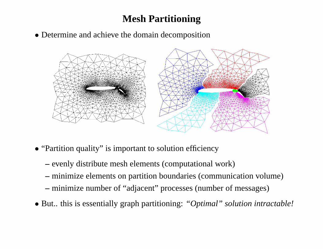
Mesh Partitioning
• Determine and achieve the domain decomposition
• “Partition quality” is important to solution efficiency
– evenly distribute mesh elements (computational work)
– minimize elements on partition boundaries (communicationvolume)
– minimize number of “adjacent” processes (number of messages)
• But.. this is essentially graph partitioning:“Optimal” solution intractable!
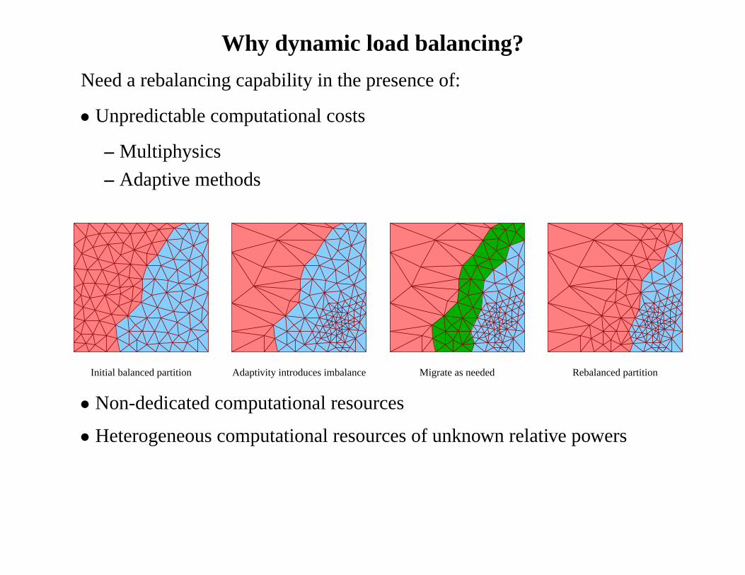
Why dynamic load balancing?
Need a rebalancing capability in the presence of:
• Unpredictable computational costs
– Multiphysics
– Adaptive methods
Initial balanced partition Adaptivity introduces imbalance Migrate as needed Rebalanced partition
• Non-dedicated computational resources
• Heterogeneous computational resources of unknown relative powers
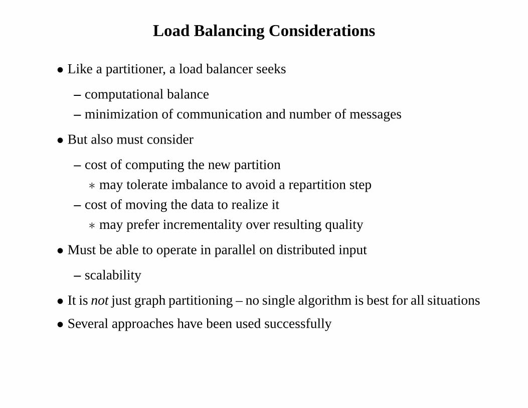
Load Balancing Considerations
• Like a partitioner, a load balancer seeks
– computational balance
– minimization of communication and number of messages
• But also must consider
– cost of computing the new partition
∗ may tolerate imbalance to avoid a repartition step
– cost of moving the data to realize it
∗ may prefer incrementality over resulting quality
• Must be able to operate in parallel on distributed input
– scalability
• It is not just graph partitioning – no single algorithm is best for allsituations
• Several approaches have been used successfully
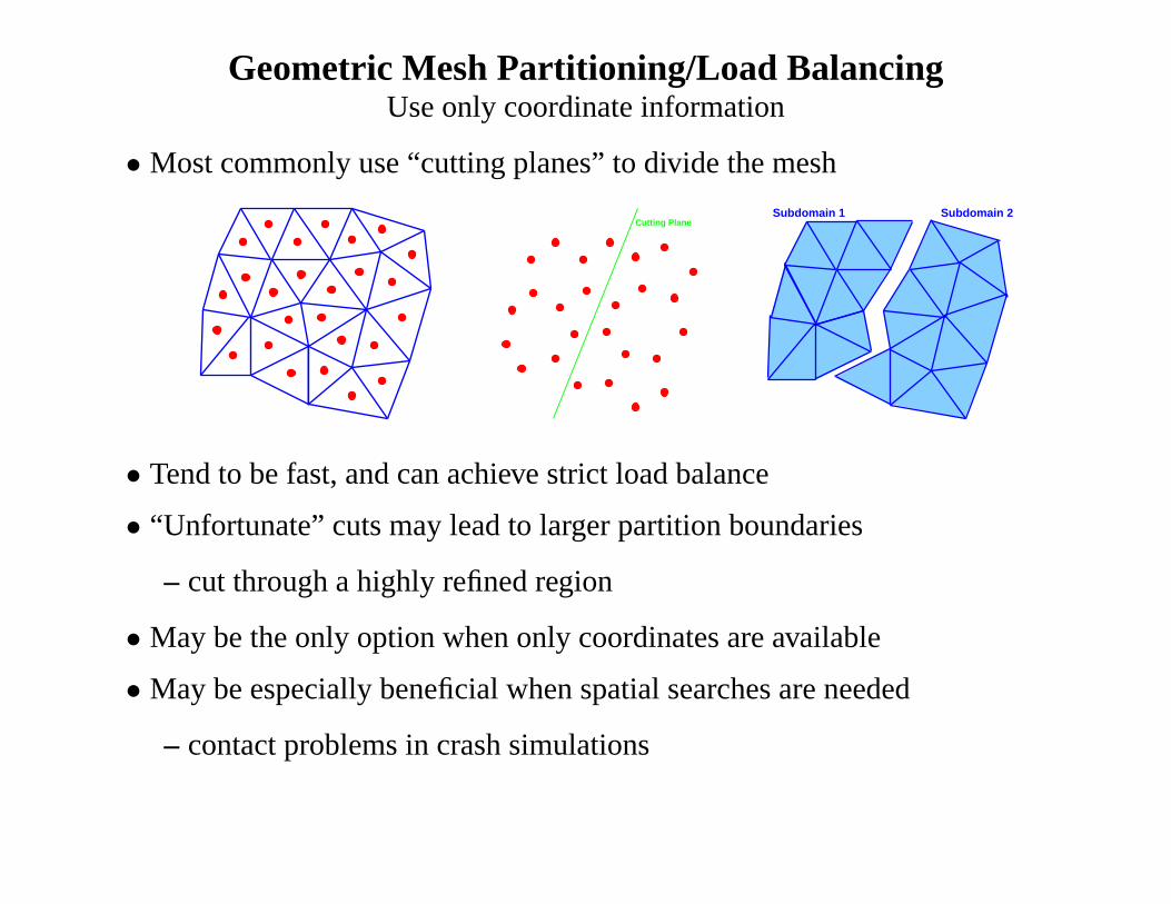
Geometric Mesh Partitioning/Load BalancingUse only coordinate information
• Most commonly use “cutting planes” to divide the mesh
Cutting PlaneSubdomain 2Subdomain 1
• Tend to be fast, and can achieve strict load balance
• “Unfortunate” cuts may lead to larger partition boundaries
– cut through a highly refined region
• May be the only option when only coordinates are available
• May be especially beneficial when spatial searches are needed
– contact problems in crash simulations
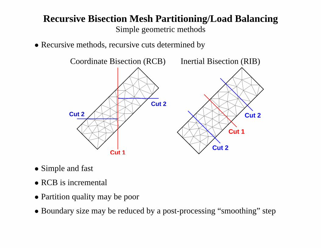
Recursive Bisection Mesh Partitioning/Load BalancingSimple geometric methods
• Recursive methods, recursive cuts determined by
Coordinate Bisection (RCB) Inertial Bisection (RIB)
Cut 2
Cut 2
Cut 1
Cut 1
Cut 2
Cut 2
• Simple and fast
• RCB is incremental
• Partition quality may be poor
• Boundary size may be reduced by a post-processing “smoothing” step
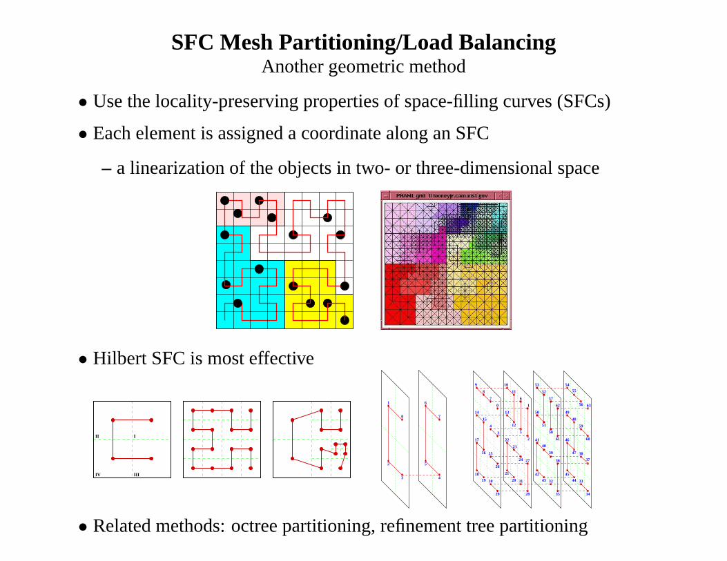
SFC Mesh Partitioning/Load BalancingAnother geometric method
• Use the locality-preserving properties of space-filling curves (SFCs)
• Each element is assigned a coordinate along an SFC
– a linearization of the objects in two- or three-dimensionalspace
• Hilbert SFC is most effective
II I
IIIIV
7
5
1
0
2
3 4
6
�����
��������
������
���
��
���
���� 37
45
55
61
58
40
39
42
20
12
18
6356
54
49
48
59
60
3847
46
44 33
3435
3243
36
41
51
50
62
57
52
53
1
6
11
10
13
5
222
23
24 27
28
31
21
3019
26
2516
17
3
4
15
14
0
7
8
9
29
������
��������
��������
����������
� �� ��� !!
""##$$%%
&&&'''(())
**++,,--
. .. .//
0 00 0112233
44556677
8899::;;
<<<===
> >> >??@ @@ @AA
BBCCDDEE
FFFGGGHHII
JJKKLLMM
N NN NOO
P PP PQQRRSS
TTUUVVWW
XXYYZZ[[
\\\]]]
^^ __`` aa
bbccddee
fffggghhii
jjkkllmm
n nn noo
p pp pqqrrss
ttuuvvww
xxyyzz{{
| || |}}
~ ~~ ~��� �� ���
��������
����������
��������
� �� ���
• Related methods: octree partitioning, refinement tree partitioning
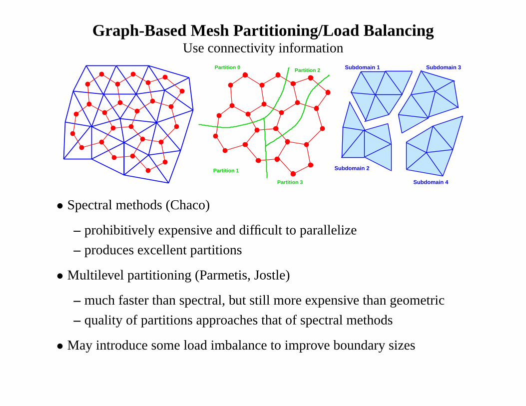
Graph-Based Mesh Partitioning/Load BalancingUse connectivity information
Partition 3
Partition 0
Partition 1
Partition 2
Subdomain 4
Subdomain 2
Subdomain 1 Subdomain 3
• Spectral methods (Chaco)
– prohibitively expensive and difficult to parallelize
– produces excellent partitions
• Multilevel partitioning (Parmetis, Jostle)
– much faster than spectral, but still more expensive than geometric
– quality of partitions approaches that of spectral methods
• May introduce some load imbalance to improve boundary sizes
Load Balancing Algorithm Implementations
• Again, no single algorithm is best in all situations
• Some are difficult to implement
• Bad: implementation within an application or framework
– likely usable only by a single application
– at best, usable by a few applications that share common data structures
– unlikely that an expert in load balancing is the developer
• Better: implementation within reusable libraries
– load balancing experts can develop and optimize implementations
– application programmers can make use without worrying about details
– but...how to deal with the variety of applications and data structures?
∗ require specific input and output structures– applications must construct them
∗ data-structure neutral design– applications only need to provide a small set of callback functions
Zoltan Toolkit
Includes suite of partitioning algorithms, developed at
• General interface to a variety of partitioners and load balancers
• Application programmer can avoid the details of load balancing
• Interact with application through callback functions and migration arrays
– “data structure neutral” design
• Switch among load balancers easily; experiment to find what works best
• Provides high quality implementations of:
– Coordinate bisection, Inertial bisection
– Octree/SFC partitioning (with Loy, Gervasio, Campbell – RPI)
– Hilbert SFC partitioning
– Refinement tree balancing (Mitchell – NIST)
– Hypergraph partitioning
• Provides easier-to-use interfaces for:
– Metis/Parmetis (Karypis, Kumar, Schloegel – Minnesota)
– Jostle (Walshaw – Greenwich)
• Freely available:http://www.cs.sandia.gov/Zoltan/

Zoltan Toolkit Interaction with Applications
callbacks invoked by Zoltan
Create Zoltan object
continue computationmigrate application data
Application Zoltan
Zoltan_Create()
Zoltan_Set_Param()
Zoltan_LB_Partition()
return migration arrayspartitioncall application callbacks
Zoltan balancer
Set parameters
Invoke balancing
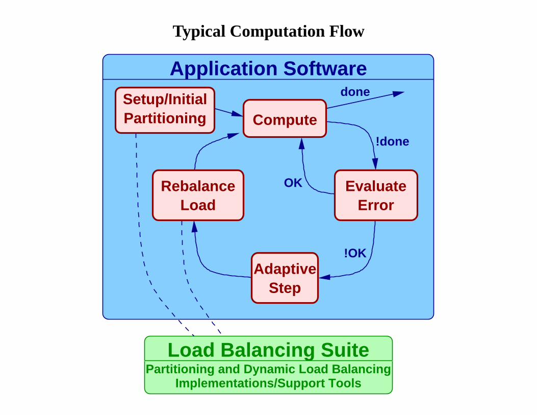
Typical Computation Flow
Implementations/Support Tools
LoadRebalance
StepAdaptive
ErrorEvaluate
ComputePartitioningSetup/Initial
Application Softwaredone
!done
OK
!OK
Load Balancing SuitePartitioning and Dynamic Load Balancing
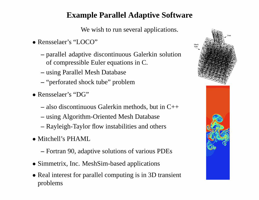
Example Parallel Adaptive Software
We wish to run several applications.
• Rensselaer’s “LOCO”
– parallel adaptive discontinuous Galerkin solutionof compressible Euler equations in C.
– using Parallel Mesh Database
– “perforated shock tube” problem
• Rensselaer’s “DG”
– also discontinuous Galerkin methods, but in C++
– using Algorithm-Oriented Mesh Database
– Rayleigh-Taylor flow instabilities and others
• Mitchell’s PHAML
– Fortran 90, adaptive solutions of various PDEs
• Simmetrix, Inc. MeshSim-based applications
• Real interest for parallel computing is in 3D transientproblems
ShockTube
Vent
Target Computational Environments
• FreeBSD Lab, Williams CS: 12 dual hyperthreaded 2.4 GHz IntelXeonprocessor systems
• Bullpen Cluster, Williams CS: 13 node Sun cluster, total of 4 300 MHz and21 450 MHz UltraSparc II processors
• Dhanni Cluster, Williams CS: 14 nodes, 8 with 2 hyperthreaded 2.8 GHzIntel Xeon processors, 2 with 2 dual-core hyperthreaded 2.8 GHz IntelXeon processors, 1 with dual hyperthreaded 2.4 GHz Intel Xeonproces-sor (compile node), and 3 with 1 1GHz Intel Pentium III
• Medusa Cluster, RPI: 32 dual 2.0GHz Intel Xeon processor systems
• ASCI-class supercomputers: large clusters of SMPs
• Grid computers – “clusters of clusters” or “clusters of supercomputers”
This is just a small sample of the wide variety of systems in use.
• long-term “resource-aware computation” goal: software that can run effi-ciently on any of them
• work described here is one step toward this goal, current focus on systemsfound at places like Williams
Resource-Aware Computing Motivations
• Heterogeneous processor speeds
– seem straightforward to deal with
– does it matter? computation proceeds only as fast as theslowestprocess
• Distributedvs. shared memory
– some algorithms may be a more appropriate choice than others
• Non-dedicated computational resources
– can be highly dynamic, transient
– will the situation change by the time we can react?
• Heterogeneous or non-dedicated networks
• Hierarchical network structures
– message cost depends on the path it must take
• Relative speeds of processors/memory/networks
– important even when targeting different homogeneous clusters
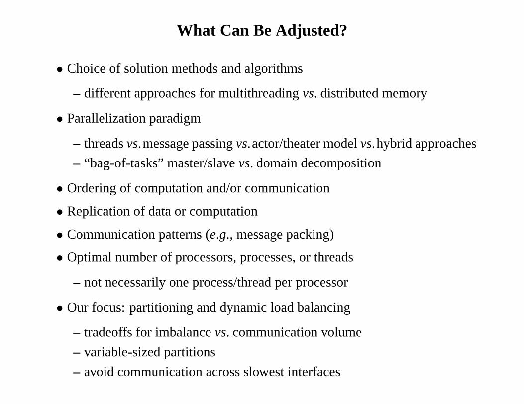
What Can Be Adjusted?
• Choice of solution methods and algorithms
– different approaches for multithreadingvs. distributed memory
• Parallelization paradigm
– threadsvs.message passingvs.actor/theater modelvs.hybrid approaches
– “bag-of-tasks” master/slavevs. domain decomposition
• Ordering of computation and/or communication
• Replication of data or computation
• Communication patterns (e.g., message packing)
• Optimal number of processors, processes, or threads
– not necessarily one process/thread per processor
• Our focus: partitioning and dynamic load balancing
– tradeoffs for imbalancevs. communication volume
– variable-sized partitions
– avoid communication across slowest interfaces
Bullpen Cluster at Williams College
2 CPUs @ 450MHz
512 MB memory
512 MB memory2 CPUs @ 450MHz
arroyo
rivera
mendoza
128 MB memory1 CPU @ 300MHz
4 CPUs @ 450MHz
1 CPU @ 300MHz128 MB memory
nelson
4 GB memory
1 CPU @ 300MHz128 MB memory
lloyd
wetteland
1 CPU @ 333MHz128 MB memory
stanton
4 CPUs @ 450MHz
1 GB memory1 CPU @ 450MHz
bullpen
4 GB memory
Net
wo
rk (
100M
bit
Eth
ern
et)
1 GB memory
righetti2 CPUs @ 450MHz512 MB memory
mcdaniel2 CPUs @ 450MHz
gossage
512 MB memory2 CPUs @ 450MHz
lyle
2 CPUs @ 450MHz
1 GB memory
farr
All nodes contain (aging) Sun UltraSparc II processors
http://bullpen.cs.williams.edu/
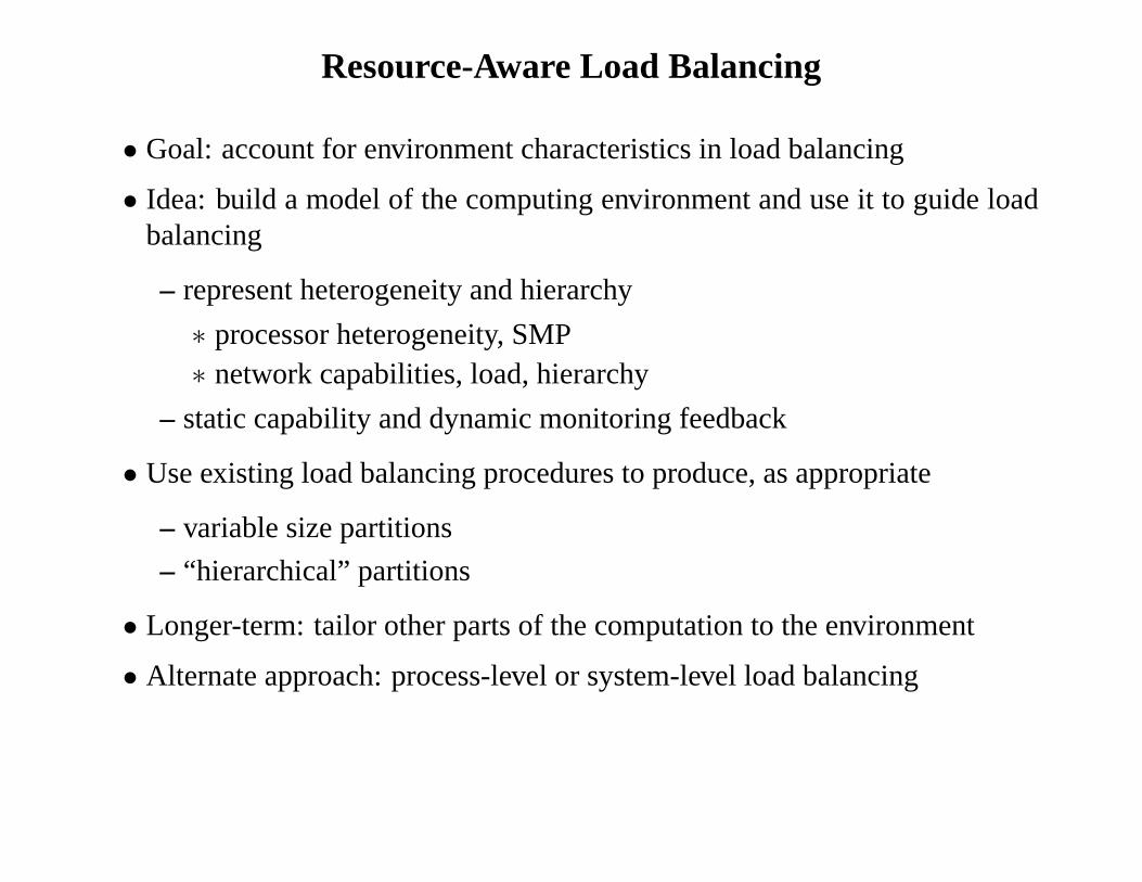
Resource-Aware Load Balancing
• Goal: account for environment characteristics in load balancing
• Idea: build a model of the computing environment and use it toguide loadbalancing
– represent heterogeneity and hierarchy
∗ processor heterogeneity, SMP∗ network capabilities, load, hierarchy
– static capability and dynamic monitoring feedback
• Use existing load balancing procedures to produce, as appropriate
– variable size partitions
– “hierarchical” partitions
• Longer-term: tailor other parts of the computation to the environment
• Alternate approach: process-level or system-level load balancing
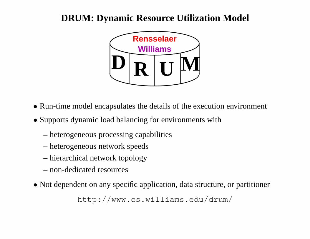
DRUM: Dynamic Resource Utilization Model
MRensselaer
Williams
D R U
• Run-time model encapsulates the details of the execution environment
• Supports dynamic load balancing for environments with
– heterogeneous processing capabilities
– heterogeneous network speeds
– hierarchical network topology
– non-dedicated resources
• Not dependent on any specific application, data structure, or partitioner
http://www.cs.williams.edu/drum/

Computation Flow with DRUM monitoring
!OK
Application Softwaredone
!done
OK
!OK
Load Balancing SuitePartitioning and Dynamic Load Balancing
Implementations/Support Tools
Setup/InitialPartitioning Compute
EvaluateError
AdaptiveStep
RebalanceLoad
StaticCapabilities
DynamicMonitoring
PerformanceAnalysis
ResourceMonitoring
System
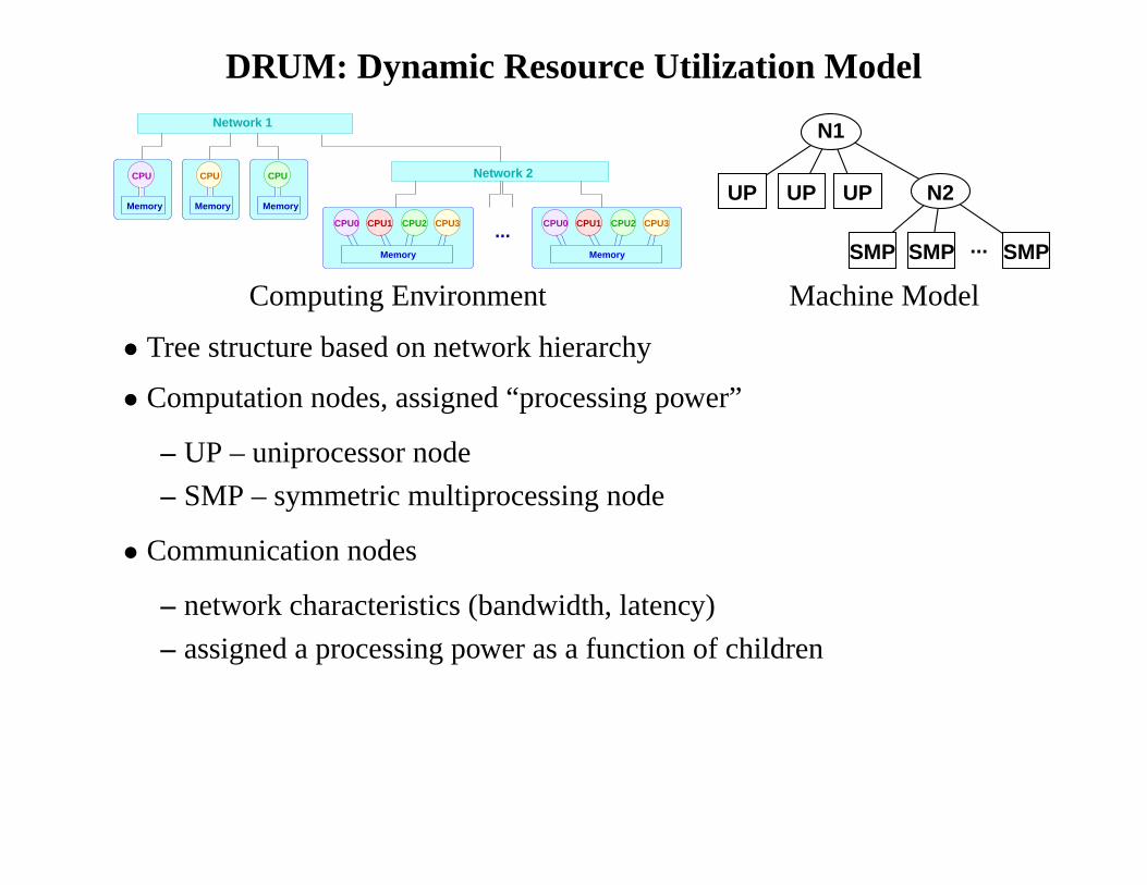
DRUM: Dynamic Resource Utilization Model
CPU CPU CPU
CPU0 ...
Network 2
CPU2CPU1 CPU3 CPU2CPU1 CPU3CPU0
MemoryMemory
Network 1
Memory
MemoryMemory
N2UP UP UP
SMP SMPSMP
N1
...
Computing Environment Machine Model
• Tree structure based on network hierarchy
• Computation nodes, assigned “processing power”
– UP – uniprocessor node
– SMP – symmetric multiprocessing node
• Communication nodes
– network characteristics (bandwidth, latency)
– assigned a processing power as a function of children
DRUM: Dynamic Resource Utilization Model
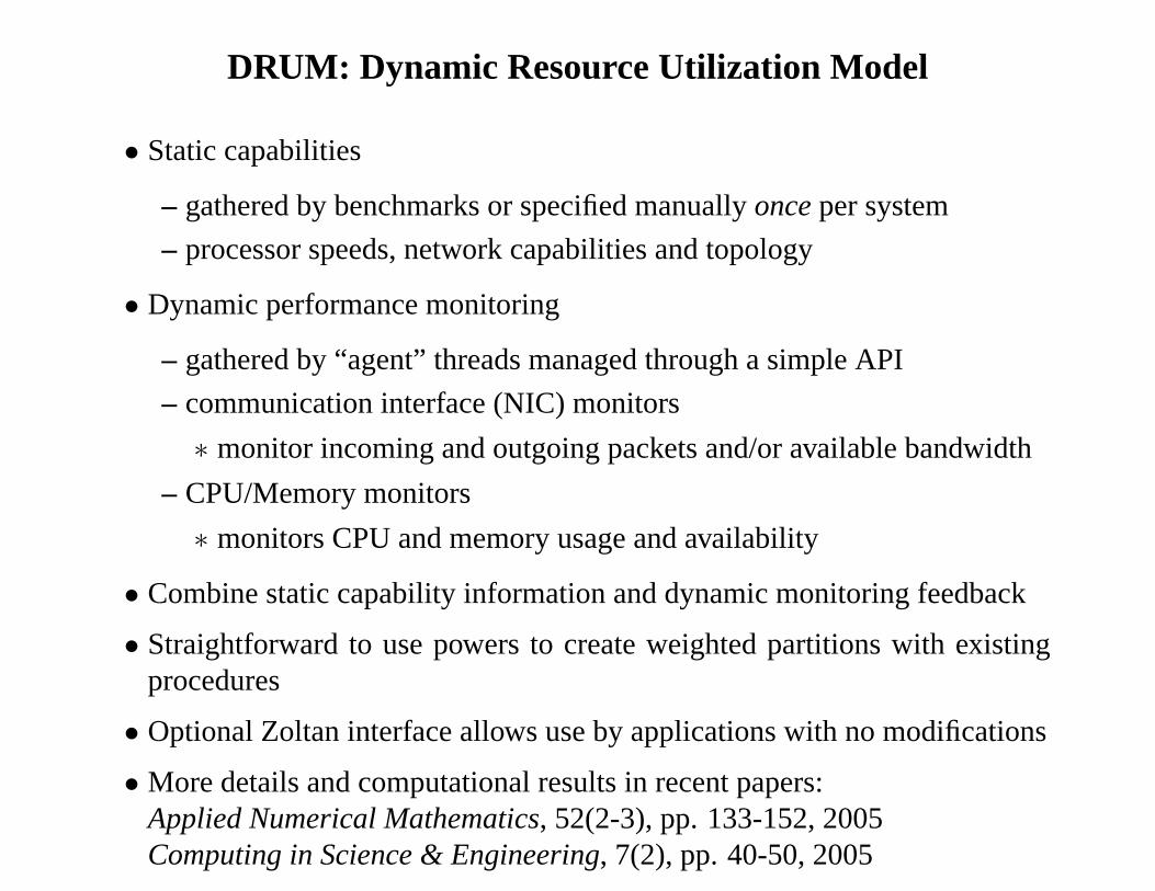
• Static capabilities
– gathered by benchmarks or specified manuallyonceper system
– processor speeds, network capabilities and topology
• Dynamic performance monitoring
– gathered by “agent” threads managed through a simple API
– communication interface (NIC) monitors
∗ monitor incoming and outgoing packets and/or available bandwidth
– CPU/Memory monitors
∗ monitors CPU and memory usage and availability
• Combine static capability information and dynamic monitoring feedback
• Straightforward to use powers to create weighted partitions with existingprocedures
• Optional Zoltan interface allows use by applications with no modifications
• More details and computational results in recent papers:Applied Numerical Mathematics, 52(2-3), pp. 133-152, 2005Computing in Science & Engineering, 7(2), pp. 40-50, 2005
DRUM Setup and Configuration
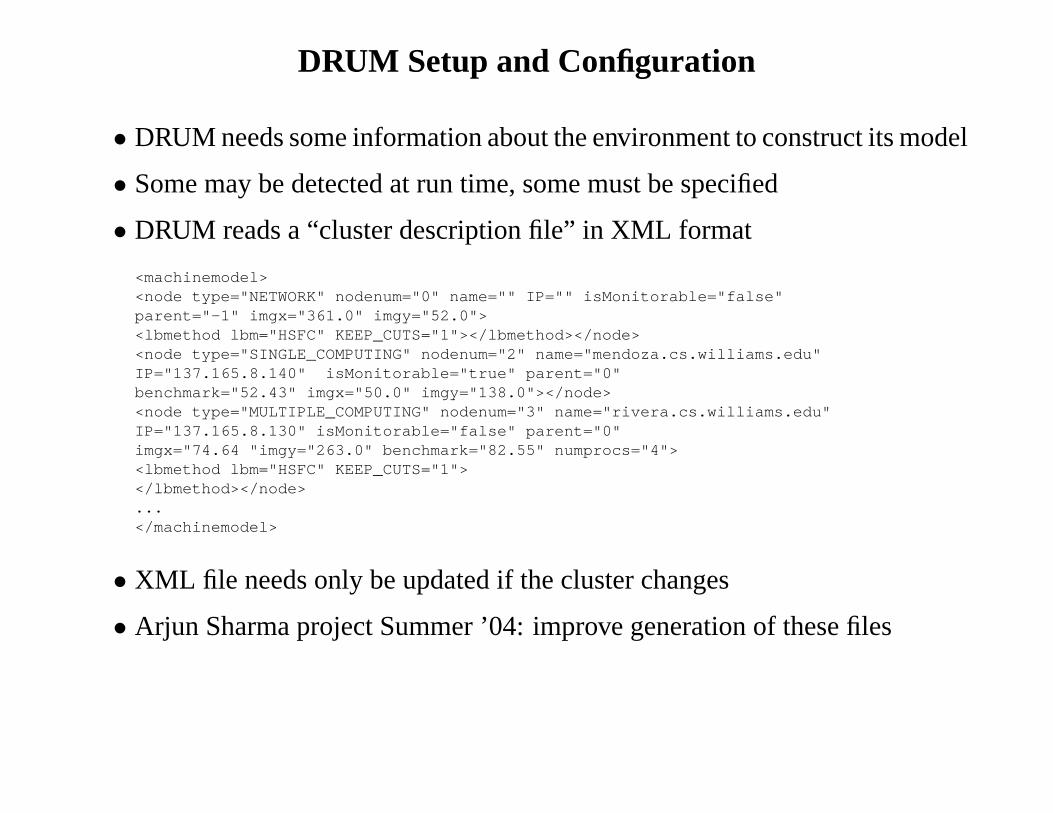
• DRUM needs some information about the environment to construct its model
• Some may be detected at run time, some must be specified
• DRUM reads a “cluster description file” in XML format
<machinemodel><node type="NETWORK" nodenum="0" name="" IP="" isMonitorable="false"parent="-1" imgx="361.0" imgy="52.0"><lbmethod lbm="HSFC" KEEP_CUTS="1"></lbmethod></node><node type="SINGLE_COMPUTING" nodenum="2" name="mendoza.cs.williams.edu"IP="137.165.8.140" isMonitorable="true" parent="0"benchmark="52.43" imgx="50.0" imgy="138.0"></node><node type="MULTIPLE_COMPUTING" nodenum="3" name="rivera.cs.williams.edu"IP="137.165.8.130" isMonitorable="false" parent="0"imgx="74.64 "imgy="263.0" benchmark="82.55" numprocs="4"><lbmethod lbm="HSFC" KEEP_CUTS="1"></lbmethod></node>...</machinemodel>
• XML file needs only be updated if the cluster changes
• Arjun Sharma project Summer ’04: improve generation of these files
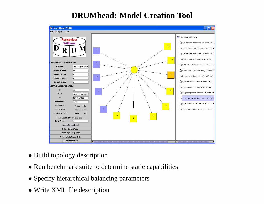
DRUMhead: Model Creation Tool
• Build topology description
• Run benchmark suite to determine static capabilities
• Specify hierarchical balancing parameters
• Write XML file description
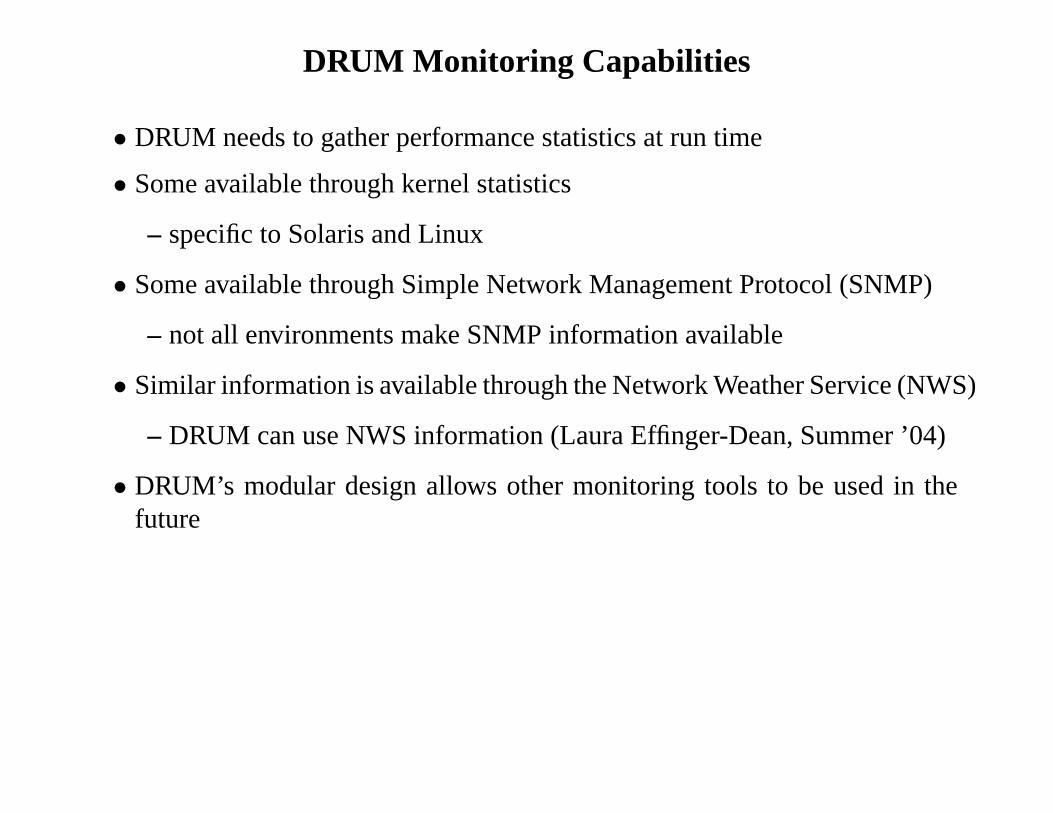
DRUM Monitoring Capabilities
• DRUM needs to gather performance statistics at run time
• Some available through kernel statistics
– specific to Solaris and Linux
• Some available through Simple Network Management Protocol (SNMP)
– not all environments make SNMP information available
• Similar information is available through the Network Weather Service (NWS)
– DRUM can use NWS information (Laura Effinger-Dean, Summer ’04)
• DRUM’s modular design allows other monitoring tools to be used in thefuture
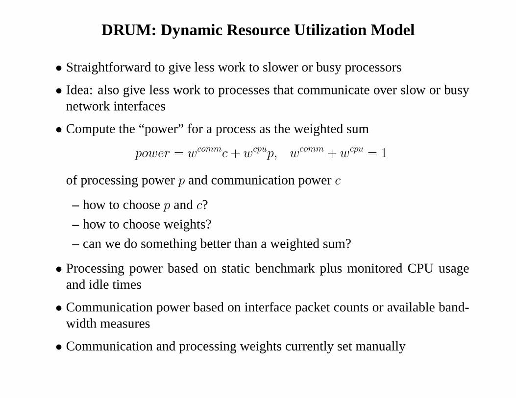
DRUM: Dynamic Resource Utilization Model
• Straightforward to give less work to slower or busy processors
• Idea: also give less work to processes that communicate overslow or busynetwork interfaces
• Compute the “power” for a process as the weighted sum
power = wcommc + wcpup, wcomm + wcpu = 1
of processing powerp and communication powerc
– how to choosep andc?
– how to choose weights?
– can we do something better than a weighted sum?
• Processing power based on static benchmark plus monitored CPU usageand idle times
• Communication power based on interface packet counts or available band-width measures
• Communication and processing weights currently set manually
DRUM: Dynamic Resource Utilization Model
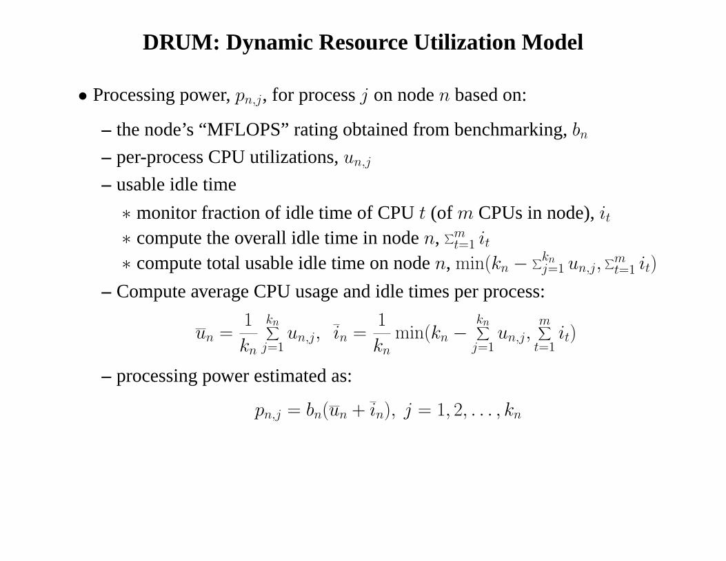
• Processing power,pn,j, for processj on noden based on:
– the node’s “MFLOPS” rating obtained from benchmarking,bn
– per-process CPU utilizations,un,j
– usable idle time
∗ monitor fraction of idle time of CPUt (of m CPUs in node),it∗ compute the overall idle time in noden, ∑m
t=1it
∗ compute total usable idle time on noden, min(kn −∑kn
j=1 un,j,∑m
t=1it)
– Compute average CPU usage and idle times per process:
un =1
kn
kn∑
j=1
un,j, in =1
kn
min(kn −kn∑
j=1
un,j,m∑
t=1
it)
– processing power estimated as:
pn,j = bn(un + in), j = 1, 2, . . . , kn
DRUM: Dynamic Resource Utilization Model
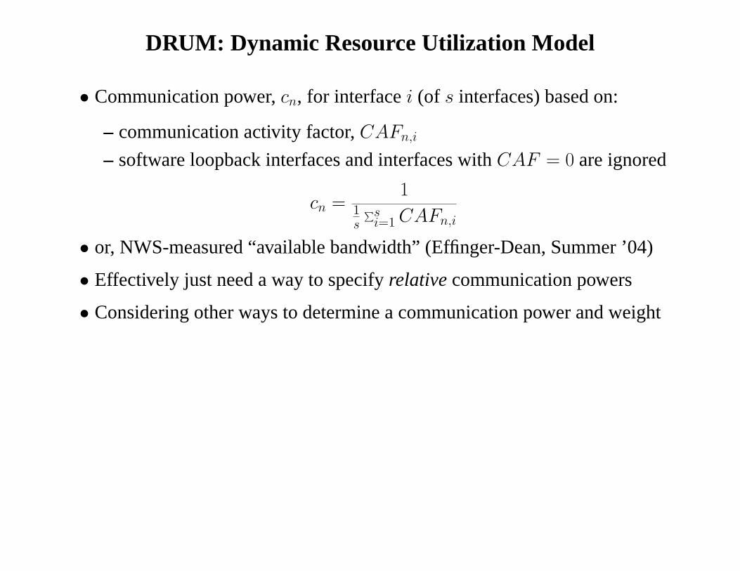
• Communication power,cn, for interfacei (of s interfaces) based on:
– communication activity factor,CAFn,i
– software loopback interfaces and interfaces withCAF = 0 are ignored
cn =1
1
s
∑si=1
CAFn,i
• or, NWS-measured “available bandwidth” (Effinger-Dean, Summer ’04)
• Effectively just need a way to specifyrelativecommunication powers
• Considering other ways to determine a communication power and weight
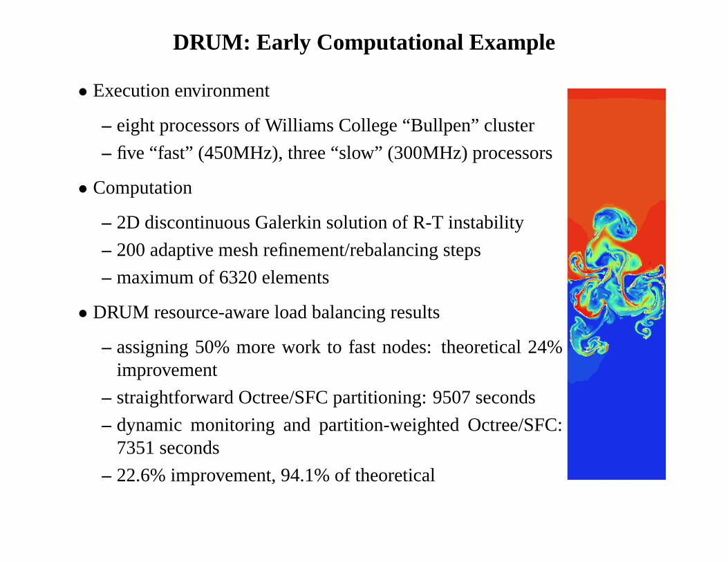
DRUM: Early Computational Example
• Execution environment
– eight processors of Williams College “Bullpen” cluster
– five “fast” (450MHz), three “slow” (300MHz) processors
• Computation
– 2D discontinuous Galerkin solution of R-T instability
– 200 adaptive mesh refinement/rebalancing steps
– maximum of 6320 elements
• DRUM resource-aware load balancing results
– assigning 50% more work to fast nodes: theoretical 24%improvement
– straightforward Octree/SFC partitioning: 9507 seconds
– dynamic monitoring and partition-weighted Octree/SFC:7351 seconds
– 22.6% improvement, 94.1% of theoretical
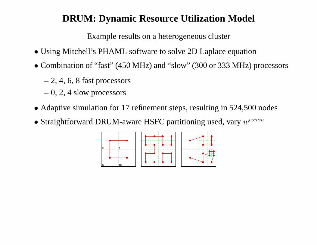
DRUM: Dynamic Resource Utilization Model
Example results on a heterogeneous cluster
• Using Mitchell’s PHAML software to solve 2D Laplace equation
• Combination of “fast” (450 MHz) and “slow” (300 or 333 MHz) processors
– 2, 4, 6, 8 fast processors
– 0, 2, 4 slow processors
• Adaptive simulation for 17 refinement steps, resulting in 524,500 nodes
• Straightforward DRUM-aware HSFC partitioning used, varywcomm
II I
IIIIV
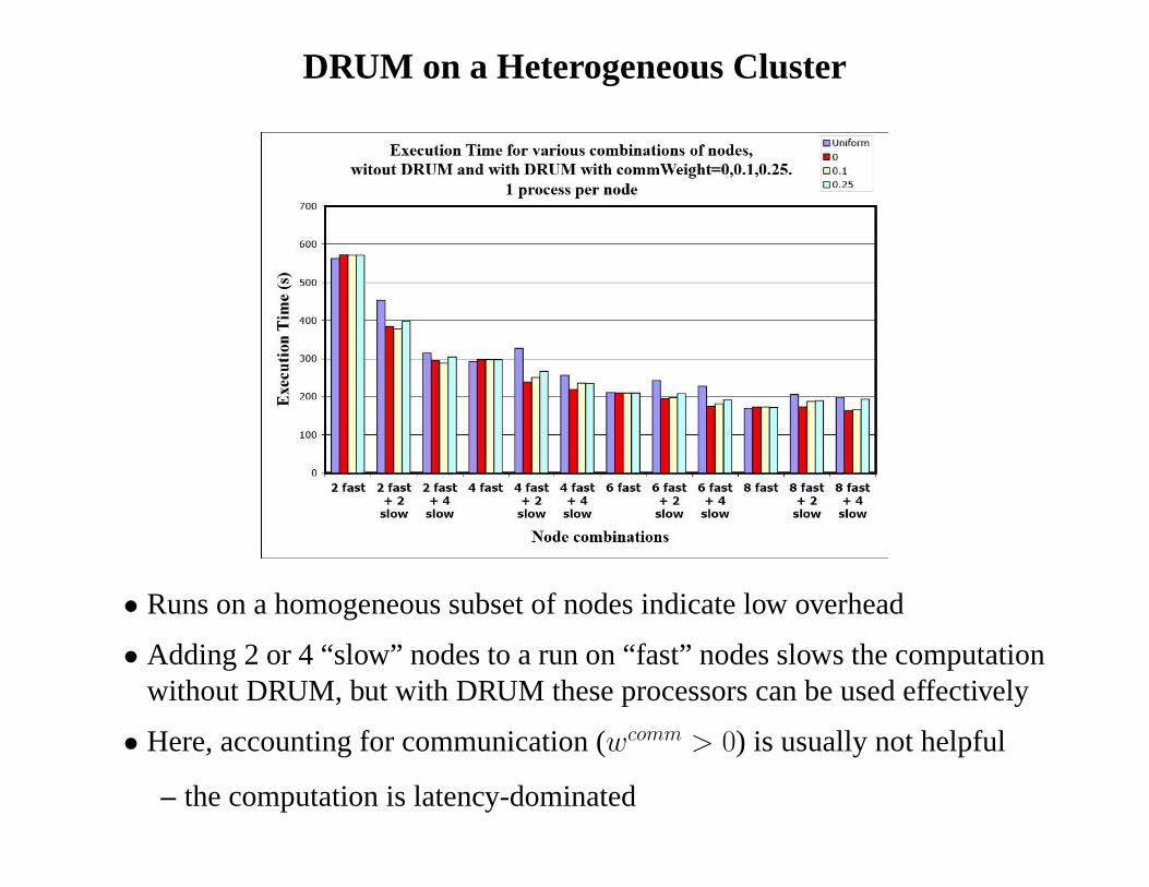
DRUM on a Heterogeneous Cluster
• Runs on a homogeneous subset of nodes indicate low overhead
• Adding 2 or 4 “slow” nodes to a run on “fast” nodes slows the computationwithout DRUM, but with DRUM these processors can be used effectively
• Here, accounting for communication (wcomm > 0) is usually not helpful
– the computation is latency-dominated
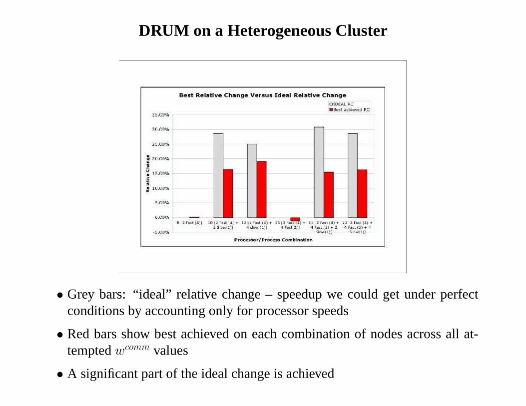
DRUM on a Heterogeneous Cluster
• Grey bars: “ideal” relative change – speedup we could get under perfectconditions by accounting only for processor speeds
• Red bars show best achieved on each combination of nodes across all at-temptedwcomm values
• A significant part of the ideal change is achieved
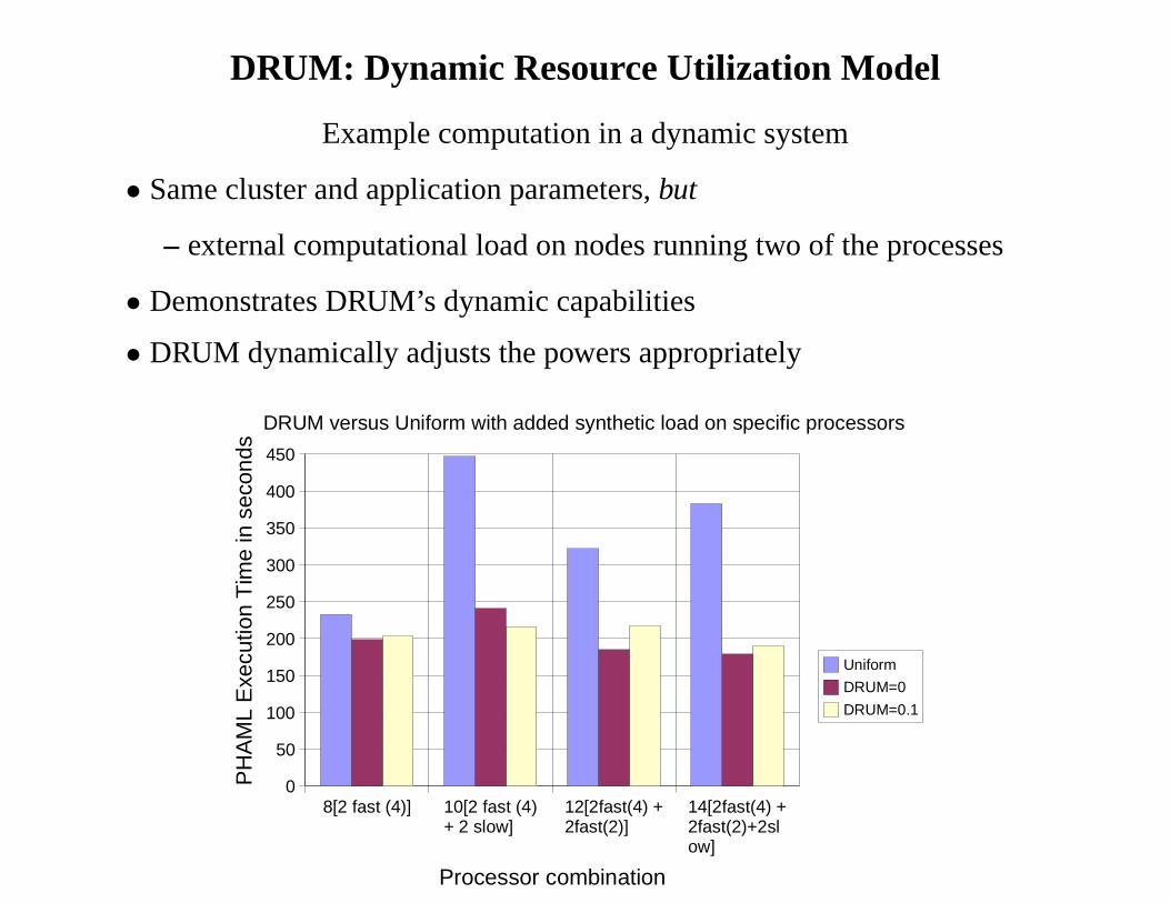
DRUM: Dynamic Resource Utilization Model
Example computation in a dynamic system
• Same cluster and application parameters,but
– external computational load on nodes running two of the processes
• Demonstrates DRUM’s dynamic capabilities
• DRUM dynamically adjusts the powers appropriately
8[2 fast (4)] 10[2 fast (4) + 2 slow]
12[2fast(4) + 2fast(2)]
14[2fast(4) + 2fast(2)+2slow]
0
50
100
150
200
250
300
350
400
450
DRUM versus Uniform with added synthetic load on specific processors
Uniform
DRUM=0
DRUM=0.1
Processor combination
PH
AM
L E
xecu
tion
Tim
e in
sec
onds
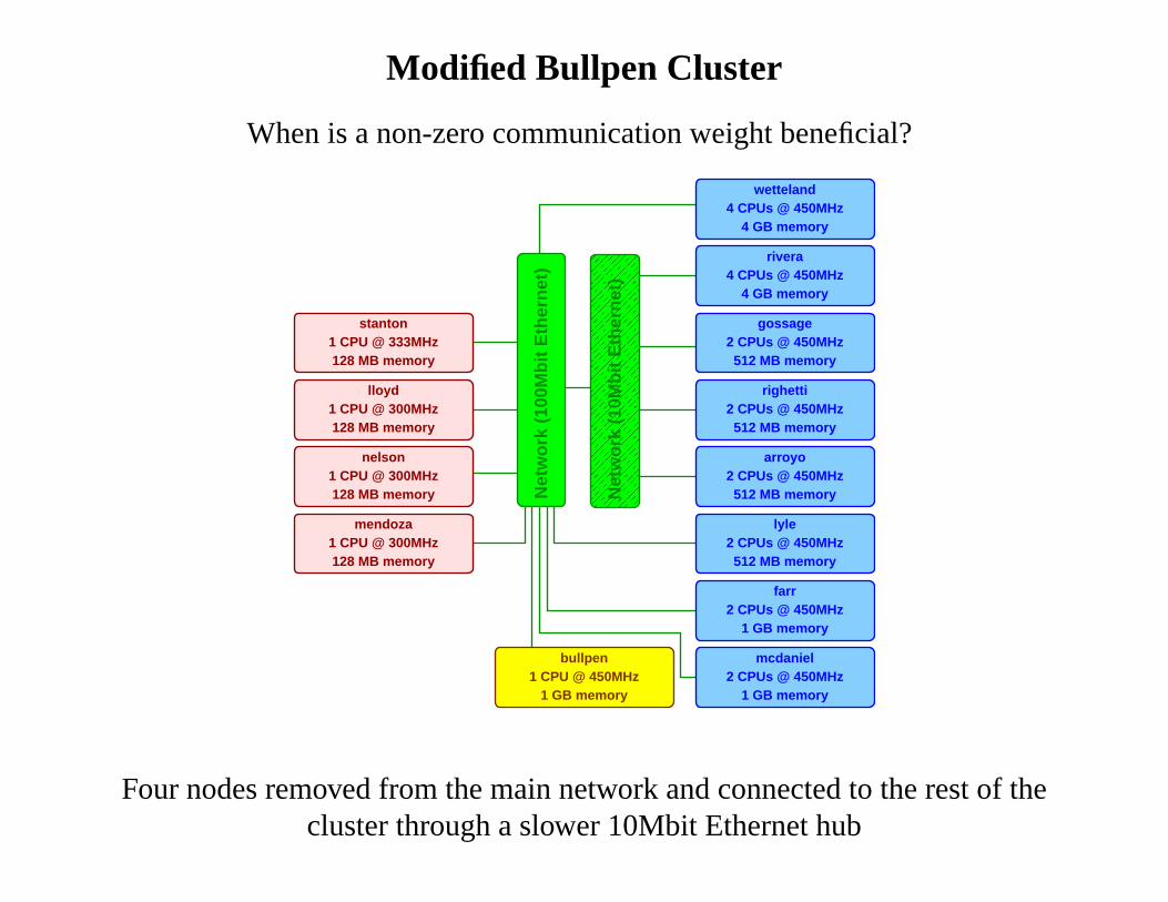
Modified Bullpen Cluster
When is a non-zero communication weight beneficial?
� � � � � �
� � � � � �
� � � � � �
� � � � � �
� � � � � �
� � � � � �
� � � � � �
� � � � � �
� � � � � �
� � � � � �
� � � � � �
� � � � � �
� � � � � �
� � � � � �
� � � � � �
� � � � � �
� � � � � �
� � � � � �
� � � � � �
� � � � � �
� � � � � �
� � � � � �
� � � � � �
� � � � �
� � � � �
� � � � �
� � � � �
� � � � �
� � � � �
� � � � �
� � � � �
� � � � �
� � � � �
� � � � �
� � � � �
� � � � �
� � � � �
� � � � �
� � � � �
� � � � �
� � � � �
� � � � �
� � � � �
� � � � �
� � � � �
4 CPUs @ 450MHz
128 MB memory
stanton
4 GB memory
1 GB memory1 CPU @ 450MHz
bullpen
1 GB memory
1 GB memory
mcdaniel2 CPUs @ 450MHz
2 CPUs @ 450MHz
512 MB memory2 CPUs @ 450MHz
arroyo
farr
Net
wo
rk (
10M
bit
Eth
ern
et)
512 MB memoryN
etw
ork
(10
0Mb
it E
ther
net
)128 MB memory
mendoza
righetti2 CPUs @ 450MHz
2 CPUs @ 450MHzlyle
512 MB memory
gossage2 CPUs @ 450MHz512 MB memory
rivera4 CPUs @ 450MHz
1 CPU @ 300MHz
4 GB memory
1 CPU @ 300MHz128 MB memory
nelson
wetteland
1 CPU @ 300MHz128 MB memory
lloyd
1 CPU @ 333MHz
Four nodes removed from the main network and connected to therest of thecluster through a slower 10Mbit Ethernet hub
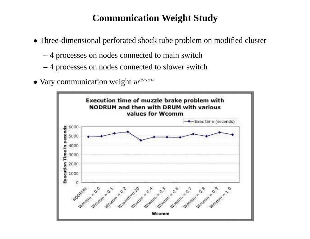
Communication Weight Study
• Three-dimensional perforated shock tube problem on modified cluster
– 4 processes on nodes connected to main switch
– 4 processes on nodes connected to slower switch
• Vary communication weightwcomm
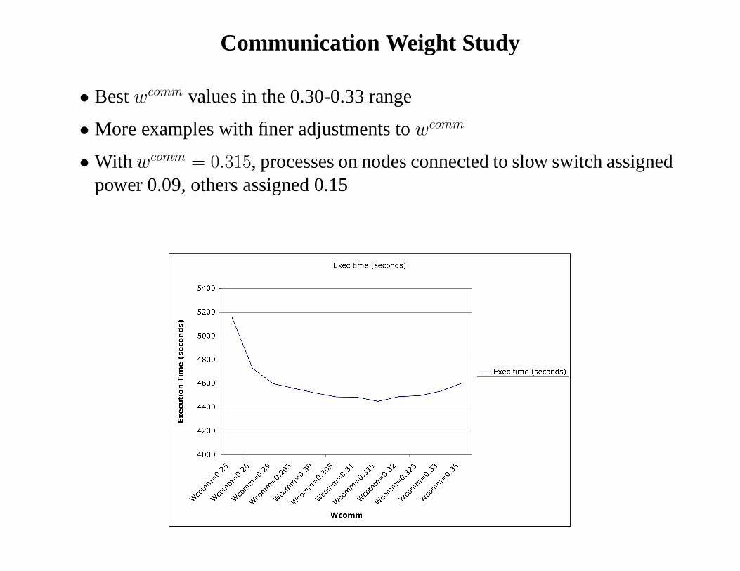
Communication Weight Study
• Bestwcomm values in the 0.30-0.33 range
• More examples with finer adjustments towcomm
• With wcomm = 0.315, processes on nodes connected to slow switch assignedpower 0.09, others assigned 0.15
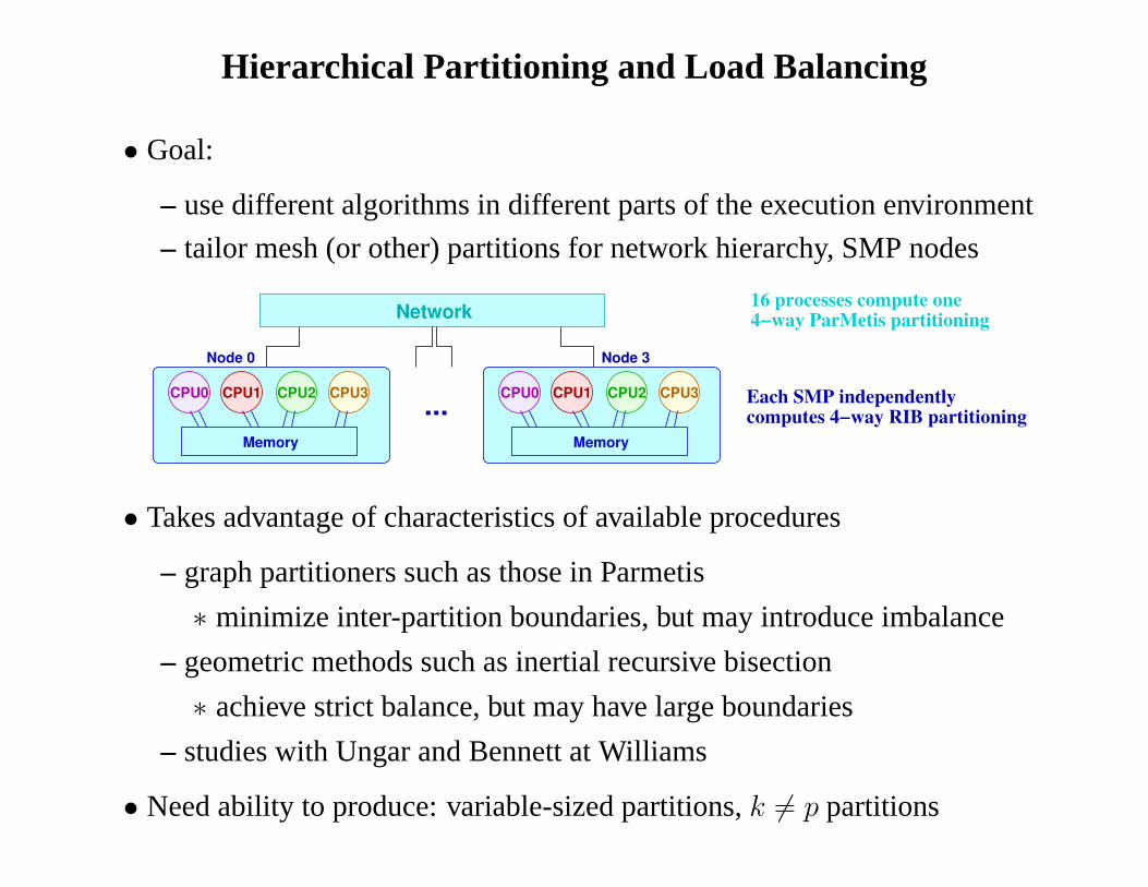
Hierarchical Partitioning and Load Balancing
• Goal:
– use different algorithms in different parts of the execution environment
– tailor mesh (or other) partitions for network hierarchy, SMPnodes
CPU0 CPU2CPU1 CPU3CPU0
Network
CPU2CPU1 CPU3
Node 0
...
Node 3
MemoryMemory
4−way ParMetis partitioning
Each SMP independentlycomputes 4−way RIB partitioning
16 processes compute one
• Takes advantage of characteristics of available procedures
– graph partitioners such as those in Parmetis
∗ minimize inter-partition boundaries, but may introduce imbalance
– geometric methods such as inertial recursive bisection
∗ achieve strict balance, but may have large boundaries
– studies with Ungar and Bennett at Williams
• Need ability to produce: variable-sized partitions,k 6= p partitions
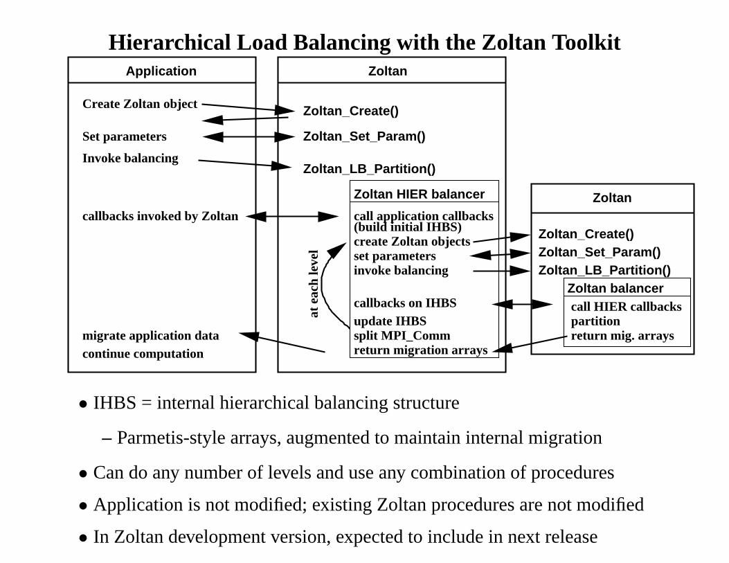
Hierarchical Load Balancing with the Zoltan Toolkit
split MPI_Comm
Zoltan_Create()Zoltan_Set_Param()Zoltan_LB_Partition()
Zoltan balancer
Zoltan
call HIER callbackspartitionreturn mig. arrays
Create Zoltan object
Application Zoltan
Zoltan_Create()
Zoltan_Set_Param()
Zoltan_LB_Partition()
Zoltan HIER balancer
Set parameters
Invoke balancing
callbacks invoked by Zoltan
continue computationmigrate application data
callbacks on IHBS
set parameterscreate Zoltan objects
call application callbacks
at e
ach
leve
l
invoke balancing
(build initial IHBS)
return migration arrays
update IHBS
• IHBS = internal hierarchical balancing structure
– Parmetis-style arrays, augmented to maintain internal migration
• Can do any number of levels and use any combination of procedures
• Application is not modified; existing Zoltan procedures arenot modified
• In Zoltan development version, expected to include in next release
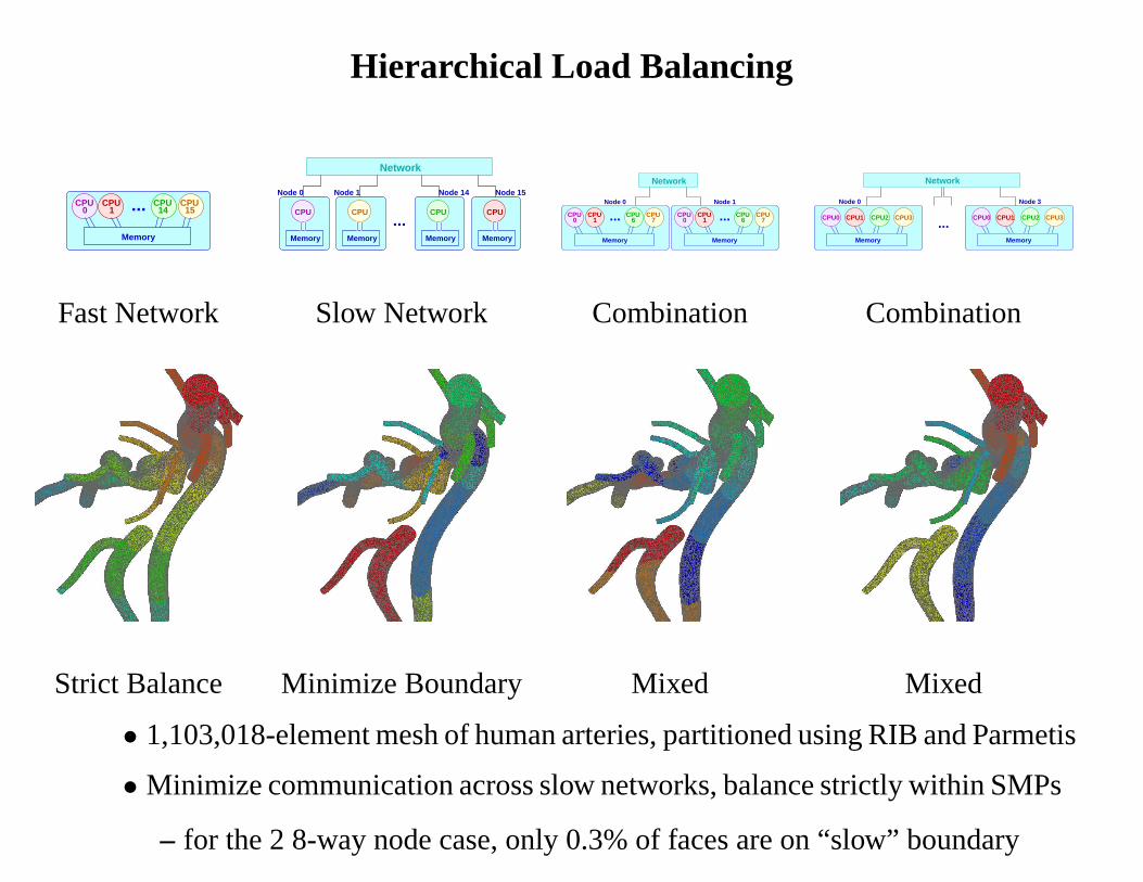
Hierarchical Load Balancing
CPU0 1
CPU CPU15
CPU14...
Memory Memory
CPU
Network
CPU
Memory Memory
CPU
Memory
CPU
Node 0 Node 15Node 1 Node 14
... CPU1
CPUCPUCPU7
Network
...0CPU
0CPU
1 6CPU
7
Memory
CPU6...
Node 0 Node 1
Memory
CPU1 CPU3CPU2CPU0 CPU2
Network
CPU1 CPU3
Memory
CPU0
Memory
Node 0 Node 3
...
Fast Network Slow Network Combination Combination
Strict Balance Minimize Boundary Mixed Mixed
• 1,103,018-element mesh of human arteries, partitioned usingRIB and Parmetis
• Minimize communication across slow networks, balance strictly within SMPs
– for the 2 8-way node case, only 0.3% of faces are on “slow” boundary
Dhanni Cluster at Williams College
1 Pentium III@1GHzdhanni10
512 MB memory1 Pentium III@1GHz
dhanni9
1 GB memory2 HTT [email protected]
cdhanni (compile node)
1 GB memory2 DC+HTT [email protected]
dhanni11
1 GB memory2 DC+HTT [email protected]
dhanni12
To Campus Network
Net
wo
rk (
Gig
abit
Eth
ern
et) 1 GB memory
2 HTT [email protected]
1 GB memory2 HTT [email protected]
dhanni3
1 GB memory2 HTT [email protected]
dhanni4
1 GB memory2 HTT [email protected]
dhanni5
1 GB memory2 HTT [email protected]
dhanni6
1 GB memory2 HTT [email protected]
dhanni7
1 GB memory2 HTT [email protected]
dhanni8
256 MB memory1 CPU @ 1GHz
cscluster
1 GB memory2 HTT [email protected]
dhanni1
512 MB memory
Legend: DC=dual core, HTT=hyperthreadedBlue nodes have 4 logical processors, red nodes have 8 logical processors
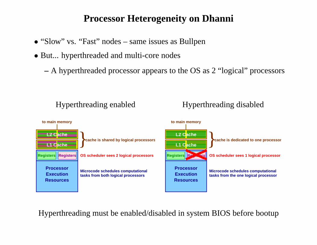
Processor Heterogeneity on Dhanni
• “Slow” vs. “Fast” nodes – same issues as Bullpen
• But... hyperthreaded and multi-core nodes
– A hyperthreaded processor appears to the OS as 2 “logical” processors
Hyperthreading enabled Hyperthreading disabled
L2 Cache
tasks from both logical processors
Registers Registers
ProcessorExecutionResources
OS scheduler sees 2 logical processors
L1 Cache } cache is shared by logical processors
to main memory
Microcode schedules computational
cache is dedicated to one processor
tasks from the one logical processorMicrocode schedules computational
Registers OS scheduler sees 1 logical processorRegisters
ProcessorExecutionResources
L2 Cache
L1 Cache }to main memory
Hyperthreading must be enabled/disabled in system BIOS before bootup
Processor Heterogeneity on Dhanni
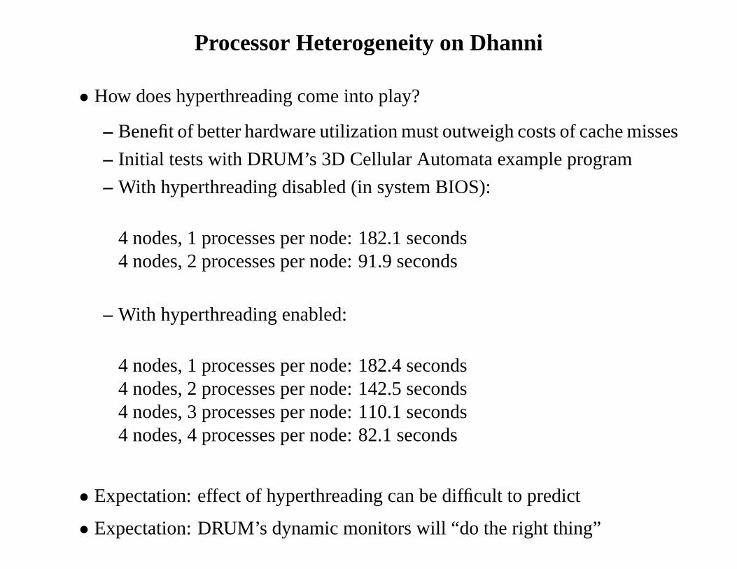
• How does hyperthreading come into play?
– Benefit of better hardware utilization must outweigh costs of cache misses
– Initial tests with DRUM’s 3D Cellular Automata example program
– With hyperthreading disabled (in system BIOS):
4 nodes, 1 processes per node: 182.1 seconds4 nodes, 2 processes per node: 91.9 seconds
– With hyperthreading enabled:
4 nodes, 1 processes per node: 182.4 seconds4 nodes, 2 processes per node: 142.5 seconds4 nodes, 3 processes per node: 110.1 seconds4 nodes, 4 processes per node: 82.1 seconds
• Expectation: effect of hyperthreading can be difficult to predict
• Expectation: DRUM’s dynamic monitors will “do the right thing”
Ongoing and Future Work in DRUM
• Apply DRUM to other applications ([email protected])
• Further DRUM management of the computation – triggering load balancing
• Prepare a public release of DRUM (currently available by request)
• Apply to Grid environments
– more heterogeneity: more need for and more benefit from DRUM
– more hierarchy: hierarchical balancing
– take advantage of other Grid-aware discovery and monitoring tools
• Hyperthreaded and dual-core nodes
– test current DRUM version in these environments
– enhance DRUM for such environments – discovery, benchmarks
– hierarchical partitions?
Balancing at Other Levels
• Process-level load balancing
– migrate MPI processes among computing nodes
– developing middleware MPI/IOS system with Varela and ElMaghraoui(RPI)
∗ uses MPI-2 functionality to migrate MPI processes∗ migrate processes only at “convenient” times for the application using
Process Checkpoint and Migration (PCM) library
– migration is expensive
– support for transient environments
• System-level load balancing
– migrate entire virtual operating systems, enabled by Xen project
– migration is expensive, but migrating systems can continueoperatinguntil the final step
– just-completed senior honors thesis by Travis Vachon
– initial focus on data center environments, but is this appropriate for HPCapplications?
Closing Remarks
• Accounting for heterogeneity and hierarchy can improve efficiency
• DRUM and hierarchical balancing software are not dependenton specificapplication software or mesh structures
– DRUM is a standalone library (but works well with Zoltan)
– HIER is part of the Zoltan Toolkit
• DRUM and hierarchical balancing can be transparent to applications
• Tools like DRUM more important in more heterogeneous environments
• Heterogeneity was intentional here but will arise over timeas nodes areadded to clusters
– “one man’s trash is another man’s new cluster node”
– multi-core and hyperthreaded processors
– also think of networks of workstations, grid environments
• Focus to date on application-level load balancing, but process- and system-level balancing may be appropriate in some circumstances
AcknowledgementsFirst, thank you for having me here today and for your attention.
The primary funding for initial DRUM development and for the hierarchical partitioning anddynamic load balancing work has been through Sandia National Laboratories by contract15162 and by the Computer Science Research Institute. Sandia is a multiprogram labora-tory operated by Sandia Corporation, a Lockheed Martin Company, for the United StatesDepartment of Energy’s National Nuclear Security Administration under contract DE-AC04-94AL85000.
Portions of this work have also been supported by the following sponsors:• Williams College Summer Science Program • Simmetrix, Inc.
Computer systems used include:
• The “Bullpen Cluster” of Sun servers and FreeBSD lab at Williams College
• The “Dhanni Cluster” of Linux servers at Williams College
• Workstations and multiprocessors at Sandia National Laboratories and Rensselaer Poly-technic Institute
• The PASTA Laboratory at Union College (long, long ago)