Inflation Risk Premium: Evidence from the TIPS Market∗

Olesya V. GrishchenkoPenn State University

Jing-zhi HuangPenn State University

First draft: August 2007This version: December 2007

Abstract

We study the term structure of real interest rates, expected inflation and in-flation risk premia using data on prices of Treasury inflation-protected securities(TIPS) over the period 2000-2006. Our study is motivated by the importance ofthe information inferred from TIPS securities. In particular, Bernanke (2004)stressed that “inflation-indexed securities would appear to be the most directsource of information about inflation expectations and real interest rates”. Wefind that inflation risk premium is time varying and more specifically, negativein the first half of the sample but is positive in the second half of the sample.The negative inflation risk premium during 2000-2003 appears to be due to liq-uidity problems in the TIPS market. We estimate that the mean inflation riskpremium over the second half of the sample is about 9 and 24 basis points over5- and 10-yr horizons, respectively, when we use the Survey of Professional Fore-casters for 10-year expected inflation measure. We also find that inflation riskpremium is considerably less volatile during 2004-2006, a finding consistent withthe observation that inflation expectations is more stable during this period.

∗Both authors are at Smeal College of Business, Penn State University, University Park, PA 16802. E-mail: ovg1@psu.edu and jxh56@psu.edu. We thank John Williams and Matthew Cocup of the BarclaysCapital Index Products Team and Rael Limbitco, US Fixed Income Strategist at Barclays Capital in NewYork, for generously providing us with TIPS data. We also thank Marco Rossi for his great researchassistance. Corresponding author: Olesya Grishchenko.

Inflation Risk Premium: Evidence from the TIPS Market

Abstract

We study the term structure of real interest rates, expected inflation and inflation risk

premia using data on prices of Treasury inflation-protected securities (TIPS) over the period

2000-2006. Our study is motivated by the importance of the information inferred from TIPS

securities. In particular, Bernanke (2004) stressed that “inflation-indexed securities would

appear to be the most direct source of information about inflation expectations and real

interest rates”. We find that inflation risk premium is time varying and more specifically,

negative in the first half of the sample but is positive in the second half of the sample. The

negative inflation risk premium during 2000-2003 appears to be due to liquidity problems

in the TIPS market. We estimate that the mean inflation risk premium over the second

half of the sample is about 9 and 24 basis points over 5- and 10-yr horizons, respectively,

when we use the Survey of Professional Forecasters for 10-year expected inflation measure.

We also find that inflation risk premium is considerably less volatile during 2004-2006, a

finding consistent with the observation that inflation expectations is more stable during this

period.

1 Introduction

Treasury Inflation-Protected Securities (TIPS) were first issued by the U.S. Treasury de-

partment in 1997. Since then, the TIPS market has grown substantially to about 8% of the

outstanding Treasury debt. One important feature of this indexed debt is that both the

principal and coupon payments from TIPS are linked to the value of an official price index

- the Consumer Price Index (CPI). Namely, both payments from TIPS are denominated in

real rather than nominal terms. As such, TIPS can be considered to be free of inflation

risk. The difference between nominal Treasury and TIPS yields of equivalent maturities

is known as a breakeven inflation rate1 and represents the compensation to investors for

bearing the inflation risk. This compensation includes both the expected inflation and the

inflation risk premium (due to inflation uncertainty). In 2004, Ben Bernanke in his speech

before The Investment Analysis Society of Chicago stressed that estimating the magnitude

of the inflation risk premium2 is important for the purpose of deriving the correct measure

of market participants’ expected inflation. Indeed, having a good estimate of inflation risk

premium is important for both demand and supply sides of the economy. On the demand

side, such a measure would allow investors to hedge effectively against inflation risk. On

the supply side, the measure would allow Treasury to tune the supply of the TIPS. As

Greenspan (1985) stated, “... The real question with respect to whether indexed debt will

save taxpayer money really gets down to an evaluation of the size and persistence of the

so-called inflation risk premium that is associated with the level of nominal interest rates.”

However, inflation risk premium is not directly observable and is known to be difficult

to be estimated accurately. The literature on estimating the magnitude and volatility of

inflation risk premium is also rather limited. The usual way to estimate inflation risk

premium in the literature is to use the difference between nominal long-term and short-

term yields, so called term premium. In this paper, we take a different approach. We

estimate the inflation risk premium using market prices of TIPS. Our use of TIPS market

prices was motivated by the view of Bernanke (2004) who stated that “...the inflation-

indexed securities would appear to be the most direct source of information about inflation

expectations and real rates”. More specifically, in our empirical analysis we use monthly

yields on zero-coupon TIPS with maturities of 5, 7, and 10 years from Barclays Capital,

and monthly yields on zero-coupon nominal Treasury bonds from Federal Reserve over the1More formally, we define a breakeven inflation rate as a difference between nominal and real yields and

we call a TIPS breakeven rate the difference between nominal and TIPS yields of the same maturity.2See Bernanke (2004).

3

period 2000-2006. As such, unlike those obtained in the existing studies, our estimates of

inflation risk premium are derived directly from TIPS trading data.

We estimate that the mean inflation risk premium is about 9 basis points and 24 basis

points over 5- and 10-yr horizons, respectively. In addition, we find that inflation risk

premium is time varying and more specifically, is negative in the first half of the sample

but is positive in the second half of the sample. The negative inflation risk premium during

2000-2003 appears to be due to liquidity problems in the TIPS market. We also find that

inflation risk premium is considerably less volatile during 2004-2006, a finding consistent

with the observation that inflation expectations is more stable during this period. We

explicitly adjust the inflation risk premium for liquidity in TIPS which is proxied by the

average trading volume and bid-ask spreads. Once we adjust the inflation risk premium for

liquidity, its estimates drop to about 14 basis points. These estimates are not unreasonable

given the Bernanke (2004)’s view that inflation risk premium of 35 to 100 basis points are

too large.

The most related study to ours is by D’Amico, Kim, and Wei (2006) who estimate

a three-factor term structure model and conclude that TIPS yields contain a substantial

“liquidity” component. However, the long-run averages of inflation risk premium in their

study can be positive or negative depending upon the different series that they use to fit a

three-factor term-structure model. The estimates of inflation risk premium that we obtain

are much lower than the ones obtained by Campbell and Shiller (1996), Buraschi and Jiltsov

(2005), and Ang, Bekaert, and Wei (2007b). For example, Campbell and Shiller (1996)

provide the estimate of inflation risk premium based on the term premium. According to

their study, inflation risk premium is between 50 and 100 basis points. In a more recent

study, Buraschi and Jiltsov (2005) analyze both nominal and real risk premia of the U.S.

term structure of interest rates based on a structural monetary version of a real business

cycle model. They find that inflation risk premium is time-varying, ranging from 20 to 140

basis points. Their estimate of the average 10-year inflation risk premium is roughly 70 basis

points over a period of 40 years. Ang, Bekaert, and Wei (2007b) estimate a term structure

model with regime switches and find that the unconditional five-year inflation risk premium

is around 1.15%, but its estimates vary with regimes. However, the results in these studies

may not be directly comparable because the sample period, estimation methods and data

sets are different.

Other studies that use TIPS data to estimate term structure models are Jarrow and

Yildirim (2003) and Chen, Liu, and Cheng (2005), but their focus is different.

4

We follow the methodology in a spirit of Evans (1998), where we employ equilibrium

first order conditions to link the nominal and real term structures. Evans (1998) uses

these equilibrium conditions in order to test the Fisher hypothesis using U.K. data. He

strongly rejects Fisher hypothesis, however, he does not provide any estimates of inflation

risk premium in the U.K.

To summarize, our study is a first attempt to estimate US inflation risk premium using

the TIPS market prices. The rest of the paper is organized as follows. Section 2 describes

data used in our empirical analysis and methodology. Section 3 presents estimation results

for real yields, inflation risk premium and the correction for liquidity premium. Finally,

Section 4 concludes.

2 Data and Methodology

In this section we describe data used in our empirical analysis and also our methodology.

A An Overview of the TIPS Market

TIPS were first introduced in 1997. This indexed debt was initially called Treasury Inflation

Protected Securities (TIPS). Later on its official name was changed to Treasury Inflation

Indexed Securities. Nevertheless, market participants keep calling these instruments TIPS,

so we retain this abbreviation for our paper. The first TIPS debt had a maturity of 10

years. Since 1997, Treasury has been issuing regularly additional 10-year debt, and 5-year,

10-year and 30-year debt irregularly. The TIPS market has been growing significantly since

its inception, although the market had significant liquidity problems in the first few years.

For instance, In December 2005, $329 billion TIPS were outstanding, representing roughly

8% of nominal Treasury debt. Currently the average monthly trading volume of TIPS is

over $9 billion.

The main advantage of TIPS over nominal Treasuries is that TIPS investors are almost

hedged against inflation risk. The coupon rate of a TIPS is fixed in real terms, and the

principal amount grows with inflation over the life of indexed debt. The real return (pur-

chasing power) of TIPS does not vary with inflation. However, the real return of nominal

Treasury declines as inflation increases. Therefore, nominal Treasury debt holders are not

protected against inflation risk.

The following example illustrates how TIPS investors are protected against inflation

fluctuations, but nominal debt holders are not. Suppose in January 2006 Treasury auctioned

5

5-year TIPS with 2% coupon rate and 5-year nominal debt with coupon rate 4.5%. If an

investor buys the January TIPS and holds it to maturity, he will receive the real return to

his investment equal to 2%. If an investor buys nominal Treasury with 4.5% coupon rate,

his real return will depend on the level of the actual Consumer Price Index (CPI) inflation

rate. If inflation rate turns out to be 2.5%, then the real return on nominal debt will be 2%.

If instead, inflation rate turns out to be 3%, then the real return to nominal Treasury debt

will be only 1.5%. Part of the purchasing power will be eroded by higher inflation against

which nominal debtholders are not protected. To investors, the only relevant measure of

return is real rate of return, or real yield, since it measures the result of the investment in

terms of the purchasing power.

B Data

Due to the issue of low liquidity in the TIPS market prior to 2000, we limit our sample

period to be January 2000 to December 2006. For TIPS data, we use monthly yields on

zero-coupon TIPS of maturities 5, 7, and 10 years from Barclays Capital Bank. For nominal

data, we use monthly yields on nominal Treasury bonds from Federal Reserve. Figure 1

shows monthly nominal (Panel A) and TIPS (Panel B) term structure. From these graphs,

we see that both nominal and TIPS yields were decreasing steadily since the beginning of

our sample until about mid 2003 year, and then increasing again, with the volatility of

both types of yields being apparently much lower in the second half of the sample. Panel C

presents a TIPS breakeven rate derived as a difference between 10-year nominal and TIPS

zero-coupon yields. Clearly, the breakeven rate was relatively low and volatile in the first

half of the sample and relatively high and less volatile in the second half.

To link the TIPS and nominal Treasury bond markets, we need to use expected inflation

data. We use three measures of expected inflation. Two of them are based on historical

average of realized inflation. Namely, we use seasonally-unadjusted Consumer Price Index

(CPI) as well as Core CPI (Consumer Price Index Less Food and Energy). Our choice of

seasonally unadjusted CPI is motivated by the fact that TIPS are linked to this index (more

precisely, this index lagged 3 months). Another measure of expected inflation used in our

analysis is the expected inflation reported by Survey of Professional Forecasters conducted

by Federal Reserve Bank of Philadelphia every quarter. Ang, Bekaert, and Wei (2007a)

study various models of expected inflation and find that, after all, survey measures forecast

inflation the best.3

3Although the frequency of nominal and TIPS yields is monthly, Survey of Professional Forecasts delivers

6

Panel A of Table 1 reports the summary statistics on TIPS yields. We observe that on

average TIPS yields were between 2.22% and 2.62% for 5 and 10-year index-linked bonds

respectively.

Panel B reports sample statistics for nominal Treasuries. Nominal Treasuries yields are

between 4.22% (5 year yields) and 4.92% (10 year yields) on average during our sample

period. This indicates that the spread between nominal and inflation-linked bonds was

between 2% or 2.3% depending on the maturity of the bonds. This amount is definitely

not sufficient to account for expected inflation, which was around 2.6% during our sample

period.

Panel C of Table 1 reports the statistics of various realized and expected inflation mea-

sures. As shown in the table, the realized average inflation during our sample period was

2.59%, while SPF 10-year CPI inflation rate forecast mean is 2.49% per year with standard

deviation 0.02%. This allows us to proxy SPF expected inflation by a single number, 2.5%,

at least at 10-year horizon.

C Methodology

First, we need to construct a yield curve of real interest rates. The reason is that TIPS rates

do not equal real rates since TIPS payments are linked not to the current index level at the

time of coupon and principal payments, but to the inflation index level which is lagged 3

months. This represents some additional difficulty in computing real rates, because there

is a risk of inflation shock during three months that investors are not protected against.

Therefore, we have to establish relationship between three term structures: term structure

of nominal rates, index-linked (TIPS) term structure, and term structure of real rates. In

order to construct a real yield curve from observed nominal and TIPS data, we follow Evans

(1998).

Next, we examine inflation risk premium based on nominal yields, real yields, and

expected inflation rates. In particular, we show first that the Fisher hypothesis does not

hold, and therefore, reject a zero inflation risk premium. We then estimate inflation risk

premium. Below is the detailed description of our methodology.

C.1 Notation

Before proceeding with the description, we define some notation as follows:

quarterly forecasts of inflation. In this case, we produce inflation risk premium estimates on quarterly basis.

7

Nominal Bonds. Let Qt(h) denote the nominal price of a zero-coupon bond at period

t paying $1 at period t + h. Then define the continuously compounded yield on a bond of

maturity h as

yt(h) ≡ −1h

lnQt(h). (1)

Define k-period nominal forward rate h periods forward as

Ft(h, k) ≡[

Qt(h)Qt(h + k)

]1/k

. (2)

Real Bonds. Let Q∗t (h) denote the nominal price of a zero-coupon bond at period t

paying $Pt+h

Ptat period t+h, where Pt is the (known) price level at t. Q∗

t (h) also defines the

real price of one consumption bundle at t+h. By definition, such a bond completely indexes

against future movements in price levels h periods ahead. Then define the continuously

compounded real yield on a bond of maturity h and forward rates as

y∗t (h) ≡ −1h

lnQ∗t (h) and F ∗

t (h, k) ≡[

Q∗t (h)

Q∗t (h + k)

]1/k

. (3)

Bonds with incomplete indexation. Let Q+t (h) denote the nominal price of an

index-linked (IL) zero-coupon bond at period t paying $Pt+h−l

Ptat period t + h, where l > 0

is the indexation lag. When h = l, then such a bond pays out $1 at maturity. Therefore, we

have Qt(l) = Q+t (l) in the absence of arbitrage. The yields and forward rates of IL bonds

are defined as:

y+t (h) ≡ −1

hlnQ+

t (h) and F+t (h, k) ≡

[Q+

t (h)Q+

t (h + k)

]1/k

. (4)

In this paper, we study US Treasury-Inflation Protected Securities (TIPS) whose indexation

lag is 3 months so l = 3 in our case.

C.2 Nominal, Real, and Index-Linked Term Structure

First, let’s establish relationship between nominal, IL, and real prices: Qt, Q+t , andQ∗

t . The

expressions below are given in terms of the stochastic discount factor Mt. Also, we assume

that the price index for the month t, Pt, is known in the end of the period t. This seems to

be a reasonable approximation of the US data since the index is published with a 2-week

delay only. Let Mt+1 be a random variable that prices one-period state-contingent claims.

8

In the absence of arbitrage opportunities, the one-period nominal returns for all traded

assets, i = 1, . . . , N , are given by

Et[Mt+1Rit+1] = 1, (5)

where Rit+1 is the gross return on asset i between t and t+1, Et is the expectation operator

conditioned on the information set at time t. We use (5) to find prices of nominal, real and

IL bonds. In the case of the nominal bonds, for h > 0 (5) becomes:

Qt(h) = Et[Mt+1Qt+1(h− 1)]. (6)

In case of real bonds, the nominal return at t + 1of a claim of $(Pt+h/Pt) at t + h is given

by:

Q∗t+1(h− 1)Pt+1

Pt

Q∗t (h)

. (7)

Therefore, (5) becomes:

Q∗t (h) = Et[M∗

t+1Q∗t+1(h− 1)], (8)

where M∗t+1 = Mt+1 × Pt+1

Pt.

In a similar way, we find the price of IL claims. We know that Qt(l) = Q+t (l), so need

to find prices only for IL claims with maturities h > l. In a same way as for the case of real

bonds, we can show that

Q+t (h) = Et[M∗

t+1Q+t+1(h− 1)]. (9)

Log-linearizing equations and applying Qt(0) = Q∗t (0) = 1 we have:

qt(h) = Et

h∑

i=1

mt+i +12Vt

(h∑

i=1

mt+i

), (10)

q∗t (h) = Et

h∑

i=1

m∗t+i +

12Vt

(h∑

i=1

m∗t+i

), (11)

q+t (h) = Et

∑τi=1 m∗

t+i + Etqt+τ (l) + CVt(∑τ

i=1 m∗t+i, qt+τ (l))

+12

[Vt

(∑hi=1 m∗

t+i

)+ Vt(qt+τ (l))

],

(12)

where τ ≡ h − l, Vt(·) and CVt(·, ·) represent the conditional variance and covari-

9

ance given period t information, and the lowercase letters stand for natural logarithms.

The equations are approximations in general, but hold exactly if the joint distribution for

{Mt+j , Pt+i+1/Pt+i}j>0,i>0 conditional on the period t information is log normal.

C.3 Term Structure of Real Interest Rates

Using (10), (11), (12), and definition of m∗t ≡ mt + ∆pt, we can link prices of nominal, real

and IL bonds by the following formula:

q+t = q∗t (τ) + [qt(h)− qt(τ)] + γt(τ), (13)

where τ = h− l and

γt(τ) ≡ CVt(qt+τ (l), ∆τpt+τ ). (14)

Equation(13) shows that the log price of real bonds is not only a function of nominal

prices and IL prices, but also depends on the covariance between future inflation and future

nominal prices, measured by γt(τ). Note also, that (13) is not a function of stochastic

discount factor. Last term in (13), γt(τ) represents the compensation for the risk of high

inflation. By no-arbitrage condition, the IL bond prices depend on future nominal bond

prices, qt+τ (l), and this will affect the choice between real and IL bonds. In the periods

of unexpectedly high inflation, nominal prices drop, causing negative γt(τ). Therefore, IL

bond will sell at a discount (compare to real bonds) to compensate for this risk.

Equation (13) can be rewritten in terms of yields in order to derive the estimates of the

real term structure. Let yt(h), y∗t (h), and, y+t (h) be the continuously compounded yields

for nominal, real, and IL bonds respectively. Then (13) can be rewritten:

y∗(τ) =h

τy+

t (h)− l

τft(τ, l) +

1τγt(τ). (15)

Given (15), we can estimate real yields, y∗t using IL yields, y+t , and log nominal forward

rates, ft that we observe in the data. The only variable that has to be estimated is γt(τ).

To estimate γt(τ), we follow VAR methodology proposed by Evans (1998).

We consider first-order vector-autoregression:

zt+1 = Azt + et+1, (16)

10

where z′t ≡ [∆pt, qt(l), xt], where xt is a vector of conditioning variables that can potentially

include relevant macro-variables which would affect the covariance between inflation and

nominal bond prices. For now, we just use a unit vector, so xt = 1. As a result of estimated

(16), γt(τ) is given by:

γt(τ) = i′1

τ∑

i=1

Aτ−i

i∑

j=1

Ai−jV (et+j |zt)Ai−j′

i2, (17)

where ik, k = 1, 2 is the selection vector such that ∆pt = i′1zt and qt(l) = i′2zt. The equation

(17) shows how the covariance between ∆τpt+τ and qt+τ (l) conditioned on zt defined through

the coefficient matrix A and the innovation variances V (et+j |zt).4 The VAR(1) results are

presented in Table 2. We discuss the properties and magnitude of γt(τ) in more detail in

Section 3.

C.4 Inflation Risk Premium

Consider the following equation that defines the inflation risk premium:

yt(τ) = y∗t (τ) + Etπt+τ (τ) + IRPt(τ), (18)

where πt+τ ≡ (1/τ)∆τpt+τ , and IRPt(τ) is the inflation risk premium. This equation can

be also derived from log-linear pricing equations (10), (11), (12), and (15). Equation (18)

presents a form of Fisher equation that equates the τ−period nominal yield with the yield

on a τ−period real bond plus expected inflation and an inflation risk premium IRPt(τ).

One method of estimating inflation risk premium is based on a specification of the real

pricing kernel or a representative agent model. Examples using this approach include Fisher

(1975), Benninga and Protopapadakis (1983), Evans and Wachtel (1992), and Buraschi and

Jiltsov (2005).5

We use an alternative approach here that does not require any specification of the real

pricing kernel.6 This approach is based on the following regression:4It seems that there is a typo in the derivation of γt(τ) in Evans (1998) and we present corrected formula.5In general, inflation risk premium can be positive or negative depending on how the real pricing kernel

covaries with inflation. See, for example, Evans (1998), page 211.6 This is in the spirit of Evans (1998). Even though he shows how the inflation risk premium depends

on the real pricing kernel but he does not use any specification of the real pricing kernel in his empiricalanalysis.

11

yt(τ)− y∗t (τ)−Etπt+τ (τ) = α0 + α1

[yt(τ)− yreal

t (τ)]

+ ut+τ . (19)

By definition, the left-hand side of equation is IRPt(τ). We can, therefore, examine to which

extent the changes in the yield spread, yt(τ) − yrealt (τ), are correlated with the inflation

risk premium. Also, equation (19) can be used to estimate inflation risk premium. The

empirical results for inflation risk premium are discussed in Section 3.

3 Empirical Results

In this section we present results from the empirical analysis. We present the estimates of

real yields and the estimates of inflation risk premium. In addition, in the last subsection

of the present section we control the estimates of inflation risk premium for liquidity. TIPS

market experienced liquidity problems in the first years since its inception and especially

in the first years of our sample. In this way, our estimates of inflation risk premium can be

affected by a sound liquidity component.

A Estimate of Real Yields

In order to compute real yields, we first estimate the covariance between future inflation

and future nominal bond prices given by γt(τ) in (14). We do this by estimating VAR given

in (16) and computing γt(τ) given by (17) and present the results in the Table 2. In order

to assess how γt(τ) affects the IL yields, we annualize these estimates by multiplying them

by −1200/τ . Although γt(τ) seems to manifest uniformly upward sloping term structure,

its impact, even for 10-year yields, is not large resulting in .1076 per cent to the annualized

yields.

The estimation of real yields is given in Table 3. We can see from the table that real

yields (and TIPS yields) were quite high during the period 2000-2002. For example, real

yields were as high as 4% in 2000. This finding is consistent with the fact that the TIPS

market was quite illiquid in late 90s and early 00s. But as indicated in the table, real yields

began to decrease over 2001-2005 and then increased slightly again in 2006.

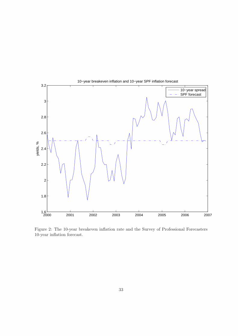
Figure 2 illustrates how the dynamics of real yields contributed to the widening of the

10-year breakeven inflation rate. It also provides the comparison between the breakeven

rate and the expected inflation provided by the Survey of Professional Forecasters. The

difference between the breakeven inflation rate and expected inflation was negative in the

12

first half of the sample period but became positive in the second half of the sample period.

It would be unreasonable to interpret this difference as a negative inflation risk premium

given the fact that many studies find positive estimates of inflation risk premium, see, for

example, Clarida and Friedman (1984), Campbell and Shiller (1996), Buraschi and Jiltsov

(2005) and Ang, Bekaert, and Wei (2007b).

Our conjecture that this difference is not entirely due to inflation risk premium, but

part of it constitutes the liquidity premium. Due to the illiquid nature of the TIPS market,

the liquidity premium, it seems, comprised a substantial component in the TIPS yields.

This factor seems to cause a breakeven inflation rate which was lower than SPF expected

inflation in the first half of our sample. In the next section, we provide the estimates of

inflation uncertainty, but they have to be treated cautiously with understanding that part

of the IRPt(τ) magnitude is due to liquidity problem. It remains to be determined how

much of the difference between breakeven rate and expected inflation was due to inflation

uncertainty and how big was the liquidity component. This is the focus of our ongoing

research.

B Estimate of the Inflation Risk Premium

We now proceed to estimate the inflation risk premium using constructed real yield curves.

In order to run regression (19), we need data on expected inflation. We proxy expected

inflation by historical averages of realized inflation based on both seasonally unadjusted

CPI and Core CPI. The average is estimated over five different windows, namely, over prior

1, 3, 5, 7, and 10 years.

Table 4 reports the estimates of historical inflation. The estimates of expected inflation

are based on seasonally unadjusted CPI show two distinguished features. First, Etπt+τ (τ)

exhibits upward-sloping term structure: that is, our estimates increase with horizon for

every estimation period. For example, for 1 year estimation period, expected inflation

increases from 2.43 percent to 2.54 percent when τ changes from 57 months (roughly 5

years) to 117 months (roughly 10 years). These estimates are consistent with the ones

obtained by other researchers. In particular, Carlstrom and Fuerst (2004) find that 10-year

expected inflation is between 2.5 and 2.6 percent. Second, for longer estimation period our

estimates are biased upward and closer to 3 per cent per year but this reflects the fact that

they encompass periods of high inflation.

Estimates of expected inflation based on Core CPI are reported in Panel B, Table 4.

As in panel A, we observe an upward sloping term structure for each estimation period,

13

and upward bias of the estimates based on a longer estimation period. At the same time,

estimates here are slightly lower than those based on the standard CPI index. On average,

the estimates of expected inflation using 1, 3, and 5 years of past inflation rates based on

Core CPI are around 2.5 per cent and consistent with what is given to us by the Survey of

Professional Forecasters.

Regression (19) shows whether inflation risk premium (IRP ) is correlated with yield

spread, yt(τ)−y∗t (τ). If it is, then Fisher hypothesis does not hold (if IRP is zero, it would

not covary with yield spreads). We obtain two sets of estimation results of inflation risk

premium using CPI and Core CPI as a proxy for inflation, and report the results in Tables 5

and 6, respectively. As can be seen from both tables, the estimates of α1 are positive and

significantly different from zero for both tables, which suggests the presence of time-varying

inflation risk premium. As such, the use of Fisher equation with IRPt(τ) is challenged, and

inflation risk premium should be taken into account when computing real yields. Evans

(1998) also documents a time-varying inflation risk premium in the UK market using UK

index-linked bonds.

Next, we compute the sample average of inflation risk premium. We use three sets

of estimates of expected inflation: (1) historical average of seasonally unadjusted CPI, to

which TIPS are linked; (2) historical average core CPI index; (3) the Survey of Professional

Forecasters (SPF) as an alternative measure of ten-year ahead forecast CPI-based inflation.

We do not use Michigan Survey of Consumers, because its one-year ahead inflation fore-

casts seem to be overestimated consistently during 2000-2006 sample period, averaging 2.84

percent. Also, Michigan survey forecasts are much more volatile than one-year forecasts by

SPF: 56 basis points vs 25 points, respectively (see Table 1, Panel C for statistics). In ad-

dition, Ang, Bekaert, and Wei (2007a) conclude that SPF has a superior ability to forecast

inflation out of sample.

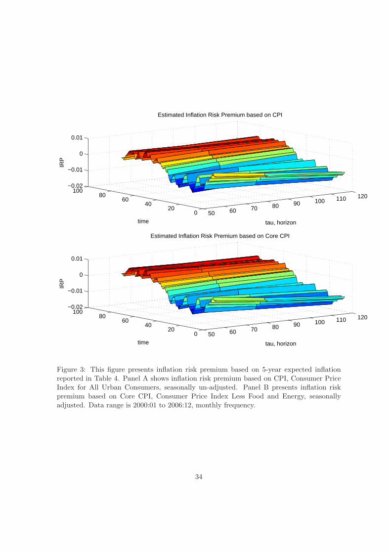
Figure 3 shows the plot of inflation risk premium both as time series and in cross section.

It reveals that inflation risk premium is visibly negative and relatively volatile in the first

half of the sample and positive and less volatile in the second half of the sample. Tables 7,

8, and 11 report sample averages for inflation risk premium based on equation (18) using

CPI, Core CPI and SPF expected inflation, respectively. Each table provides results for

the whole sample, first and second halves of the sample, and for each year. For most

proxies of expected inflation, all the tables reveal consistently that, inflation risk premium

estimates are negative during 2000-2003, the first half of the sample, and positive in the

second half. Note that IRP is negative almost everywhere (except 2006 for 5 and 7-year

14

maturity bonds) when 10-year estimation period for expected inflation is used.7 All three

sets of yearly estimates of IRPt(τ) reveal that negative inflation risk premia on average

are also due to the first half of the sample, the period 2000-2003. Recall from Table 3

that these years correspond mostly to the period of high real rates. More specifically, when

expected inflation is computed using one year of past CPI inflation rates (Table 7), the

highest inflation risk premium is 45 basis points in 2004 (on 10-year horizon). Overall,

during positive sub-period of our sample (2004-2006), inflation risk premium ranges from

10 basis points to 32 basis points (using one year estimation period for expected inflation).

When we compute inflation risk premium using Core CPI as an inflation proxy, it ranges

from 10 basis points to over 50 basis points during 2004-2006 sub-sample period. The

highest inflation risk premium is 54 basis points (on 10-year horizon): it is observed in

2006 when one-year estimation period is used for expected inflation (see Table 8). When

we use Survey of Professional Forecasters expected inflation (Table 11), we find that 5-year

inflation risk premium is the lowest among positive IRP : only 9 basis points when 10-year

CPI forecast is used. We also report that 10-year inflation risk premium is highest (42 basis

points) when one-year CPI forecast is used. These estimates are considerably lower than

the estimates obtained by Campbell and Shiller (1996), Buraschi and Jiltsov (2005) and

Ang, Bekaert, and Wei (2007b). In a related study, the long-run averages of inflation risk

premium in D’Amico, Kim, and Wei (2006) can be positive or negative depending upon the

different series that they use to fit a three-factor term-structure model.8

Tables 9 and 10 report volatility estimates for IRP . We observe that volatility in the

second half of the sample was considerably lower (across maturities) than in the first half of

the sample. For example, Table 9 shows that volatility of inflation risk premium for 10-year

bonds falls from 30 basis points to 18 basis points when expected inflation is estimated using

one year of past inflation rates. When expected inflation is estimated as a 5-year average

of past inflation rates, volatility of 10-year inflation risk premium falls from 36 basis points

to 14 basis points.

Evidence on both averages and volatilities of inflation risk premium over different hori-

zons indicates that there is a significant change in the behavior of inflation risk premium

since the end of 2003. Whether it is a structural break, and therefore, a sample is split on

two regimes remains an open question. Our on going research concerns the possibility that

shifts in liquidity in the TIPS market may explain this “structural break”. As investors7Evans (1998) notes that inflation risk premium can be positive or negative depending on how the real

pricing kernel covaries with inflation (see Evans (1998), page 211).8See Figures 4, 5 and 6 in their paper.

15

become more familiar with this new market, its liquidity seems to be gradually improving.9

In the next section we present some preliminary estimates of the inflation risk premium

controlling for liquidity effects.

C Estimating Liquidity Risk Premium

For the reasons outlined above, the estimates of inflation risk premium need to be “filtered”

from liquidity component under the assumption that the determinants of inflation risk

premium and liquidity risk premium are different. In general, we assume that the depth of

the TIPS market is closely related to the liquidity risk premium in TIPS but unlikely to

be related to the inflation risk premium. Therefore, we use bid-ask spreads of quoted TIPS

prices and trading volume data to control for liquidity effects in the inflation risk premium.

In particular, we consider the case of 10-year bonds because of the data issues with the

bonds of different maturities.10 Specifically, we assume the following statistical model

IRPt(τ) = α0 + α1spreadt(τ) + α2volumet(τ) + ut(τ), (20)

where spreadt(τ) is the average bid-ask spread of the outstanding 10-year TIPS issues,

and volumet(τ) is the log trading volume averaged across both on-the-run and off-the-run

10-year TIPS issues. ut(τ) is the residual of the inflation risk premium not explained by

liquidity variables. We run this regression for quarterly inflation risk premium which was

estimated using expected inflation from the Survey of Professional Forecasters.11 The cor-

responding IRP estimates are reported in Table 11. The reason we use quarterly estimates

of inflation risk premium is that we view them as the most reliable since Ang, Bekaert, and

Wei (2007a) show that surveys provide the best forecasts of inflation.

The regression (20) results are reported in Table 12. In the first row we present the

estimates of Model I, where we restrict α2 = 0 and use only the average bid-ask spread as

the explanatory variable for the magnitude of IRPt(τ). We interpret the regression residual

as part of the inflation risk premium not explained by TIPS liquidity issues. In the last

two columns of the table we report the average residual for both the first and the second

half of the sample. Recall from Table 3 that the first half of the sample period corresponds9There are also tax considerations that might have affected the development of the TIPS market. See,

for example, Hein and Mercer (2003) for a discussion.10We do not have a continuous time series for volume and bid-ask spreads for 5-year bonds because there

were no outstanding 5-year TIPS between July 2002 and September 2004.11We compute quarterly bid-ask spreads as average of weekly spreads within a particular quarter.

16

to the period of high real yields (10-year yields in 2000-2003 were on average 3.11%) and

the second half of the sample corresponds to the period of much lower real yields(10-year

yields in 2004-2006 were on average 1.98%). Given relatively flat curve of expected inflation

during these periods (Table 1, Panel C), it follows that negative inflation risk premium12 in

the first half of the sample is due to high real yields that seem, in part due to the liquidity

problems with TIPS market at that time. We observe lower real yields and positive inflation

risk premium during 2004-2006.13 Because the expected inflation was pretty flat during this

time period, we conjecture that lower real yields are associated with lower liquidity risks on

the TIPS market, albeit still present. This is the reason that we report the average residual

for both subperiods that is “liquidity-free” estimate of inflation risk premium for each of

the considered regression models that account for liquidity risk. In the case of Model I the

part of 10-year inflation risk premium, not explained by bid-ask spread is only 16.1, not 24

basis points, the inflation risk premium not adjusted for inflation. In the second row of the

Table 12 we report the results of the regression model II where we use log trading volume

in 10-year TIPS as a proxy for liquidity and restrict α1 = 0. In this case the adjusted

inflation risk premium is 17.6 basis points. The R2 = .335 in case of Model I and .283 in

case of Model II. Both proxies are statistically significant. Next, we report the results of

the regression Model III, where we include both the log trading volume and the average

bid-ask spread as proxies for liquidity. In this case we observe that the estimates of 10-year

inflation risk premium net of liquidity premium is 14.1 basis points. It is interesting that

the average bid-ask spread drives away the log trading volume. The R2 for this regression

is .383. The average residual for all models is negative during the first half of the sample

indicating severe liquidity issues on the TIPS market. This points out that some structural

changes occurred in the TIPS market in the middle of 2003, the mid point of our sample.

4 Conclusion

This paper is the first attempt to estimate the inflation risk premium directly using the

prices of Treasury inflation-protected securities (TIPS). Using market data on prices of

TIPS over the period 2000-2006, we find that the inflation risk premium is time varying.

More specifically, it is negative in the first half of the sample but positive in the second12Average 10-year inflation risk premium during 2000-2003 was on average minus 30 basis points, see

Table 11.13Average 10-year inflation risk premium in the second half of the sample was on average 24 basis points,

see Table 11.

17

half. We estimate that the mean inflation risk premium over the second half is about 9

and 24 basis points over 5- and 10-yr horizons, respectively, when we use the Survey of

Professional Forecasters for 10-year expected inflation measure. The negative inflation risk

premium during 2000-2003 appears to be due to liquidity problems in the TIPS market,

since it seems to be driven by very high real rates at that time. We also find that inflation

risk premium is considerably less volatile during 2004-2006, a finding consistent with the

observations that inflation expectations became more stable during this period, investors

became more familiar with TIPS market and the market liquidity has gradually improved.

Once we adjust the inflation risk premium for liquidity in TIPS, we find that 10-year inflation

risk premium is on average 14 basis points during the second half of our sample. These

estimates are much lower than the ones from earlier studies.

Our empirical results on inflation risk premium estimated directly from TIPS should be

valuable for practitioners, monetary authorities and policy makers alike because they help

to assess the inflation expectations of bond-market investors.

References

Ang, A., G. Bekaert, and M. Wei, 2007a, “Do Macro Variables, Asset Markets Forecast

Inflation Better?,” Journal of Monetary Economics, forthcoming.

, 2007b, “The Term Structure of Real Rates and Expected Inflation,” Journal of

Finance, forthcoming.

Benninga, S., and A. Protopapadakis, 1983, “Real and nominal rates under uncertainty:

The Fisher theorem and the term structure,” Journal of Political Economy, 91, 856–867.

Bernanke, B., 2004, “What Policymakers Can Learn from Asset Prices,” Speech Before the

Investment Analyst Society of Chicago.

Buraschi, A., and A. Jiltsov, 2005, “Inflation Risk Premia and the Expectation Hypothesis,”

Journal of Financial Economics, 75, 429–490.

Campbell, J. Y., and R. J. Shiller, 1996, “A Scorecard for Indexed Debt,” NBER Macroe-

conomics Annual, pp. 155–197.

Carlstrom, C. T., and T. S. Fuerst, 2004, “Expected Inflation and TIPS,” Federal Reserve

Bank of Cleveland newsletter.

18

Chen, R.-R., B. Liu, and X. Cheng, 2005, “Inflation, Fisher Equation, and the Term Struc-

ture of Inflation Risk Premia: Theory and Evidence from TIPS,” Working Paper, Rutgers

University.

Clarida, R. H., and B. M. Friedman, 1984, “The Behavior of U.S. Short-Term Interest Rates

since October 1979,” Journal of Finance, 39, 671–682.

D’Amico, S., D. H. Kim, and M. Wei, 2006, “Tips from TIPS: the informational content of

Treasury Inflation-Protected Security Prices,” Working paper, Federal Reserve Board.

Evans, M., 1998, “Real Rates, Expected Inflation, and Inflation Risk Premia,” The Journal

of Finance, 53(1), 187–218.

Evans, M., and P. Wachtel, 1992, “Interpreting the movements in short-term interest rates,”

Journal of Business, 65, 395–430.

Fisher, S., 1975, “The demand for indexed bonds,” Journal of Political Economy, 83, 509–

534.

Greenspan, A., 1985, “Inflation Indexing of Government Securities,” a hearing before the

Subcommittee of Trade, Productivity, and Economic Growth of the Joint Economic Com-

mittee.

Hein, S. E., and J. M. Mercer, 2003, “Are TIPS Really Tax Disadvantaged?,” Working

paper, Texas Tech University.

Jarrow, R., and Y. Yildirim, 2003, “Pricing Treasury Inflation Protected Securities and

Relative Derivatives using HJM Model,” Journal of Financial and Quantitative Analysis,

38(2), 337–358.

19

Table 1: Summary Statistics of Zero-Coupon TIPS, Nominal Bonds and Inflation

The table reports sample statistics for zero-coupon yields on index-linked and nominal bonds with hmonths to maturity in Panels A and B respectively. yTIPS(h) is the yield on an h-month TreasuryProtected Inflation Security (TIPS), y(h) is the yield on an h-month nominal yield. Panel C presentsrealized and expected inflation variables. Realized inflation variables are: CPI is Consumer Price Indexfor All Urban Consumers, non seasonally adjusted, and Core CPI is Consumer Price Index Less Food andEnergy, seasonally adjusted. Expected inflation variables are: 1-year forecast from Michigan ConsumerSurvey, 1-year forecast based on GDP price deflator, and 1- and 10-year forecasts based on CPI pricedeflator. Last three variables are from Survey of Professional Forecasters (SPF). Data range for allvariables is 2000:01-2006:12, monthly frequency, except SPF whose forecasts are quarterly. All numbersare in annual percentages. Source: Barclays Capital, Federal Reserve discount bonds data set, FederalReserve Bank of St. Louis Economic Data Base, and Federal Reserve Bank of Philadelphia.

Central Moments Autocorrelations

Mean Stdev Skew Kurt Lag1 Lag2 Lag3

Panel A: TIPS Yields

yTIPS(60) 2.2262 1.0061 0.4774 2.0740 0.9714 0.9443 0.9212

yTIPS(84) 2.4385 0.8989 0.5282 2.0138 0.9755 0.9521 0.9320

yTIPS(120) 2.6231 0.8077 0.5046 1.8903 0.9786 0.9583 0.9406

Panel B: Nominal Bond Yields

y(60) 4.2265 1.0187 0.4823 2.7584 0.9771 0.9552 0.9349

y(84) 4.5481 0.8374 0.6299 2.9097 0.9797 0.9605 0.9430

y(120) 4.9194 0.6724 0.6670 2.7653 0.9823 0.9657 0.9507

Panel C: Inflation Variables

CPI 2.5933 4.3513 -0.1780 3.0736 0.5215 0.1012 0.0737

Core CPI 2.1759 1.0260 0.0757 2.6381 0.8118 0.8498 0.8195

Michigan 1yr forecast 2.8440 0.5664 -0.9475 8.2099 0.9773 0.9549 0.9388

SPF, GDP 1yr forecast 2.0278 0.2220 -0.1878 1.9757 0.9583 0.9104 0.8642

SPF, CPI 1yr forecast 2.3299 0.2513 -0.7662 3.6846 0.9544 0.9092 0.8660

SPF, CPI 10yr forecast 2.4982 0.0166 -0.7062 9.1771 0.9642 0.9284 0.8927

20

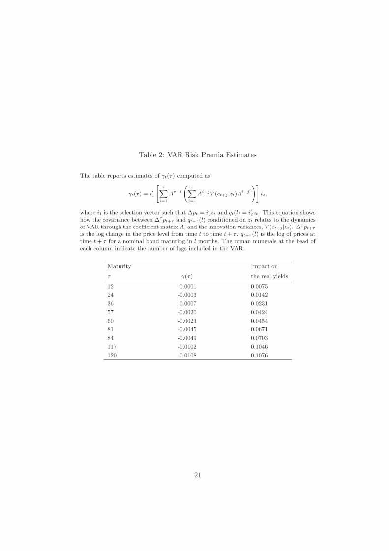
Table 2: VAR Risk Premia Estimates

The table reports estimates of γt(τ) computed as

γt(τ) = i′1

"τX

i=1

Aτ−i

iX

j=1

Ai−jV (et+j |zt)Ai−j′

!#i2,

where i1 is the selection vector such that ∆pt = i′1zt and qt(l) = i′2zt. This equation showshow the covariance between ∆τpt+τ and qt+τ (l) conditioned on zt relates to the dynamicsof VAR through the coefficient matrix A, and the innovation variances, V (et+j |zt). ∆τpt+τ

is the log change in the price level from time t to time t + τ . qt+τ (l) is the log of prices attime t + τ for a nominal bond maturing in l months. The roman numerals at the head ofeach column indicate the number of lags included in the VAR.

Maturity Impact on

τ γ(τ) the real yields

12 -0.0001 0.0075

24 -0.0003 0.0142

36 -0.0007 0.0231

57 -0.0020 0.0424

60 -0.0023 0.0454

81 -0.0045 0.0671

84 -0.0049 0.0703

117 -0.0102 0.1046

120 -0.0108 0.1076

21

Table 3: TIPS and Real Yields Statistics

The table reports statistics for TIPS yields, y+t (h), and implied real yields with h months to maturity. yreal(h) is the

real yield on an h-month zero-coupon bond, estimated using the following formula:

yreal(τ) =h

τy+

t (h)− l

τft(τ, l) +

1

τγt(τ).

Data Range: 2000:01 to 2006:12, monthly frequency. Statistics is reported for various subsamples. The estimates arebased on seasonally un-adjusted CPI, used to estimate index-linked premium reported in Table 2.

Year Horizon, TIPS Yields Real Yields

τ months Mean Stdev Skew Kurt Mean Stdev Skew Kurt

2000-2006 57 2.226 1.006 0.477 2.074 2.032 1.031 0.466 2.077

81 2.438 0.899 0.528 2.014 2.255 0.917 0.528 2.026

117 2.623 0.808 0.505 1.890 2.432 0.821 0.515 1.906

2000-2003 57 2.685 1.036 -0.154 1.729 2.495 1.064 -0.144 1.720

81 2.916 0.876 -0.190 1.755 2.734 0.901 -0.180 1.744

117 3.107 0.728 -0.244 1.787 2.919 0.747 -0.233 1.775

2004-2006 57 1.614 0.533 0.081 1.749 1.415 0.561 0.064 1.740

81 1.802 0.394 0.170 1.782 1.616 0.411 0.155 1.783

117 1.977 0.292 0.211 1.776 1.783 0.301 0.210 1.785

2000 57 3.991 0.174 0.028 2.188 3.844 0.162 0.038 2.103

81 4.001 0.176 0.109 2.299 3.855 0.171 0.097 2.262

117 3.982 0.172 0.228 2.351 3.821 0.172 0.203 2.324

2001 57 3.059 0.189 -0.289 2.677 2.879 0.194 -0.227 2.489

81 3.237 0.156 -0.420 3.019 3.064 0.158 -0.420 2.900

117 3.388 0.136 -0.399 2.805 3.206 0.137 -0.412 2.762

2002 57 2.384 0.539 -0.105 1.750 2.178 0.534 -0.086 1.769

81 2.679 0.482 -0.142 1.618 2.484 0.485 -0.129 1.616

117 2.927 0.425 -0.163 1.539 2.728 0.432 -0.152 1.533

2003 57 1.309 0.227 0.495 2.012 1.079 0.222 0.530 2.021

81 1.747 0.215 0.605 2.176 1.534 0.212 0.620 2.097

117 2.133 0.206 0.586 2.223 1.921 0.205 0.586 2.134

2004 57 1.102 0.255 -0.527 2.404 0.861 0.256 -0.643 2.533

81 1.496 0.237 -0.079 1.914 1.279 0.237 -0.147 1.991

117 1.846 0.221 0.217 1.699 1.631 0.222 0.194 1.728

2005 57 1.513 0.316 0.699 2.073 1.328 0.331 0.677 2.072

81 1.655 0.244 0.692 2.015 1.479 0.252 0.677 2.014

117 1.798 0.185 0.631 1.930 1.610 0.189 0.624 1.914

2006 57 2.227 0.177 -0.903 2.769 2.057 0.181 -0.875 2.750

81 2.256 0.169 -0.865 2.683 2.091 0.168 -0.879 2.722

117 2.289 0.171 -0.657 2.348 2.109 0.169 -0.685 2.395

22

Table 4: Expected Inflation

The table reports the estimates of the expected inflation Etπt+τ (τ) is the expected rate ofinflation computed as T−year historical average of πt+τ (τ), τ−period realized inflation. PanelA reports results using CPI, Consumer Price Index for All Urban Consumers, seasonally un-adjusted as a measure of realized inflation or Core CPI, Consumer Price Index Less Food andEnergy, seasonally adjusted.

Horizon, τ months Estimation period, T years

1 3 5 7 10

Panel A: Based on CPI

57 2.429 2.414 2.444 2.531 2.783

( 0.081) ( 0.040) ( 0.066) ( 0.155) ( 0.287)

81 2.456 2.445 2.531 2.671 2.924

( 0.141) ( 0.075) ( 0.155) ( 0.252) ( 0.284)

117 2.543 2.636 2.778 2.921 3.124

( 0.141) ( 0.225) ( 0.286) ( 0.285) ( 0.254)

Panel B: Based on Core CPI

57 2.214 2.293 2.398 2.549 2.863

( 0.140) ( 0.146) ( 0.190) ( 0.282) ( 0.380)

81 2.300 2.396 2.548 2.736 3.051

( 0.168) ( 0.204) ( 0.280) ( 0.356) ( 0.380)

117 2.509 2.673 2.859 3.049 3.327

( 0.286) ( 0.346) ( 0.380) ( 0.381) ( 0.366)

23

Table 5: Inflation Risk Premium Regressions

The table reports the estimates of inflation risk premium regression:

IRPt(τ) = α0 + α1

hyt(τ)− yreal

t (τ)i

+ ut+τ ,

where IRP is inflation risk premium computed using Consumer Price Index for All UrbanConsumers, seasonally un-adjusted as a proxy for inflation. yt(τ) is nominal τ -month yield,yreal

t (τ) is the estimate of the τ -month real yield computed from nominal and TIPS zero termstructures. t−stats are given in parentheses below.

Horizon, τ months α0 α1 R2

Etπt+τ (τ) is 1-year historical average

57 -0.023 0.930 0.978

(-33.146) (30.167)

81 -0.024 0.997 0.896

(-12.807) (10.445)

117 -0.031 1.214 0.920

(-15.888) (17.662)

Etπt+τ (τ) is 3-year historical average

57 -0.023 0.955 0.996

(-126.530) (77.325)

81 -0.026 1.091 0.980

(-40.084) (31.040)

117 -0.036 1.396 0.873

(-13.434) (14.662)

Etπt+τ (τ) is 5-year historical average

57 -0.024 0.994 0.984

(-36.321) (35.550)

81 -0.028 1.131 0.913

(-17.193) (16.765)

117 -0.042 1.561 0.859

(-13.387) (13.745)

Etπt+τ (τ) is 7-year historical average

57 -0.027 1.080 0.934

(-21.776) (18.518)

81 -0.034 1.312 0.863

(-14.007) (13.103)

117 -0.044 1.583 0.871

(-16.650) (15.033)

Etπt+τ (τ) is 10-year historical average

57 -0.034 1.271 0.874

(-16.096) (13.095)

81 -0.039 1.426 0.876

(-17.529) (14.307)

117 -0.043 1.491 0.874

(-17.567) (15.124)

24

Table 6: Inflation Risk Premium Regressions

Inflation proxy, πt+τ (τ), is measured using core inflation, Consumer Price Index Less Foodand Energy, seasonally adjusted. Otherwise the table is identical to Table 5.

Horizon, τ months α0 α1 R2

Etπt+τ (τ) is 1-year historical average

57 -0.026 1.186 0.974

(-49.039) (33.044)

81 -0.029 1.277 0.950

(-26.146) (24.896)

117 -0.038 1.544 0.851

(-13.567) (14.355)

Etπt+τ (τ) is 3-year historical average

57 -0.026 1.137 0.955

(-29.029) (22.559)

81 -0.030 1.273 0.907

(-18.722) (16.842)

117 -0.043 1.656 0.817

(-11.646) (11.826)

Etπt+τ (τ) is 5-year historical average

57 -0.027 1.158 0.925

(-21.685) (17.993)

81 -0.033 1.338 0.839

(-12.995) (12.209)

117 -0.047 1.751 0.816

(-12.504) (11.884)

Etπt+τ (τ) is 7-year historical average

57 -0.031 1.235 0.865

(-15.520) (12.779)

81 -0.038 1.483 0.814

(-12.535) (11.183)

117 -0.049 1.754 0.815

(-13.418) (11.768)

Etπt+τ (τ) is 10-year historical average

57 -0.037 1.392 0.836

(-15.004) (11.378)

81 -0.043 1.551 0.819

(-14.296) (11.306)

117 -0.051 1.711 0.816

(-14.365) (11.864)

25

Table 7: Average Inflation Risk Premium based on CPI index

The table reports the mean estimates of the inflation risk premium (IRP), computed as IRP =yt(τ) − yreal

t (τ) − Etπt+τ (τ). yt(τ) is nominal τ -month yield, yrealt (τ) is the estimate of the

τ -month real yield computed from nominal and TIPS zero term structures. Etπt+τ (τ) is theexpected rate of inflation computed as T−year historical average of πt+τ (τ), τ−period realizedinflation. CPI is seasonally un-adjusted Consumer Price Index for All Urban Consumers. DataRange: 2000:01 to 2006:12, monthly frequency. Statistics is reported for various subsamples.

Year Horizon, Estimation period, T years

τ months 1 3 5 7 10

2000-2006 57 -0.281 -0.266 -0.296 -0.383 -0.635

81 -0.201 -0.191 -0.276 -0.416 -0.669

117 -0.083 -0.176 -0.318 -0.461 -0.664

2000-2003 57 -0.577 -0.586 -0.656 -0.813 -1.178

81 -0.463 -0.511 -0.640 -0.863 -1.160

117 -0.382 -0.546 -0.744 -0.901 -1.076

2004-2006 57 0.112 0.160 0.183 0.189 0.089

81 0.149 0.236 0.209 0.180 -0.014

117 0.315 0.316 0.251 0.126 -0.116

2000 57 -0.153 -0.215 -0.375 -0.643 -1.065

81 -0.254 -0.344 -0.642 -0.920 -1.152

117 -0.549 -0.795 -0.992 -1.083 -1.259

2001 57 -0.811 -0.742 -0.849 -1.012 -1.440

81 -0.713 -0.657 -0.823 -1.086 -1.377

117 -0.570 -0.747 -0.989 -1.120 -1.277

2002 57 -0.759 -0.813 -0.840 -0.957 -1.318

81 -0.595 -0.641 -0.685 -0.903 -1.237

117 -0.340 -0.471 -0.675 -0.869 -1.038

2003 57 -0.584 -0.575 -0.558 -0.638 -0.888

81 -0.289 -0.399 -0.412 -0.543 -0.876

117 -0.068 -0.170 -0.321 -0.533 -0.730

2004 57 0.060 0.127 0.124 0.111 -0.056

81 0.353 0.279 0.215 0.163 -0.129

117 0.446 0.387 0.278 0.104 -0.135

2005 57 0.222 0.238 0.258 0.278 0.182

81 0.184 0.295 0.239 0.222 0.023

117 0.299 0.302 0.233 0.110 -0.148

2006 57 0.055 0.116 0.168 0.178 0.140

81 -0.091 0.134 0.174 0.156 0.063

117 0.200 0.260 0.242 0.164 -0.065

26

Table 8: Average Inflation Risk Premium based on Core CPI index

The table reports the mean estimates of the inflation risk premium (IRP), computed as IRP =yt(τ) − yreal

t (τ) − Etπt+τ (τ). yt(τ) is nominal τ -month yield, yrealt (τ) is the estimate of the

τ -month real yield computed from nominal and TIPS zero term structures. Etπt+τ (τ) isthe expected rate of inflation computed as T−year historical average of πt+τ (τ), τ−periodrealized inflation. CPI is seasonally un-adjusted Core Consumer Price Index for All UrbanConsumers. Data Range: 2000:01 to 2006:12, monthly frequency. Statistics is reported forvarious subsamples.

Year Horizon, Estimation period, T years

τ months 1 3 5 7 10

2000-2006 57 -0.066 -0.146 -0.250 -0.401 -0.715

81 -0.045 -0.141 -0.293 -0.481 -0.796

117 -0.049 -0.213 -0.400 -0.589 -0.867

2000-2003 57 -0.520 -0.591 -0.721 -0.934 -1.334

81 -0.453 -0.567 -0.762 -1.014 -1.356

117 -0.478 -0.684 -0.903 -1.098 -1.362

2004-2006 57 0.539 0.448 0.379 0.310 0.110

81 0.500 0.427 0.332 0.230 -0.050

117 0.523 0.413 0.272 0.089 -0.207

2000 57 -0.172 -0.327 -0.537 -0.851 -1.258

81 -0.333 -0.535 -0.850 -1.125 -1.422

117 -0.741 -0.989 -1.191 -1.356 -1.620

2001 57 -0.677 -0.762 -0.915 -1.161 -1.602

81 -0.638 -0.733 -0.969 -1.251 -1.591

117 -0.667 -0.919 -1.152 -1.336 -1.588

2002 57 -0.777 -0.781 -0.884 -1.057 -1.469

81 -0.584 -0.639 -0.782 -1.039 -1.402

117 -0.415 -0.592 -0.826 -1.035 -1.299

2003 57 -0.453 -0.492 -0.548 -0.669 -1.009

81 -0.258 -0.361 -0.449 -0.642 -1.008

117 -0.091 -0.235 -0.444 -0.664 -0.940

2004 57 0.400 0.278 0.238 0.147 -0.114

81 0.475 0.333 0.247 0.115 -0.228

117 0.532 0.383 0.218 0.005 -0.288

2005 57 0.604 0.522 0.452 0.389 0.198

81 0.534 0.463 0.357 0.263 -0.022

117 0.500 0.390 0.251 0.063 -0.238

2006 57 0.612 0.543 0.446 0.393 0.246

81 0.489 0.485 0.393 0.312 0.099

117 0.536 0.467 0.346 0.198 -0.094

27

Table 9: Volatility of Inflation Risk Premium based on CPI index

The table reports the volatility estimates of the inflation risk premium (IRP), computedas IRP = yt(τ) − yreal

t (τ) − Etπt+τ (τ). yt(τ) is nominal τ -month yield, yrealt (τ) is the

estimate of the τ -month real yield computed from nominal and TIPS zero term structures.Etπt+τ (τ) is the expected rate of inflation computed as T−year historical average of πt+τ (τ),τ−period realized inflation. CPI is seasonally un-adjusted Consumer Price Index for All UrbanConsumers. Data Range: 2000:01 to 2006:12, monthly frequency. Statistics is reported forvarious subsamples.

Year Horizon, Estimation period, T years

τ months 1 3 5 7 10

2000-2006 57 0.489 0.497 0.521 0.581 0.706

81 0.437 0.457 0.491 0.586 0.632

117 0.428 0.506 0.570 0.574 0.540

2000-2003 57 0.419 0.399 0.373 0.351 0.377

81 0.349 0.311 0.299 0.329 0.327

117 0.297 0.330 0.356 0.326 0.314

2004-2006 57 0.230 0.212 0.207 0.214 0.224

81 0.264 0.196 0.167 0.170 0.178

117 0.177 0.152 0.137 0.135 0.132

2000 57 0.392 0.333 0.326 0.295 0.313

81 0.326 0.271 0.242 0.242 0.264

117 0.176 0.169 0.191 0.195 0.187

2001 57 0.373 0.381 0.364 0.350 0.342

81 0.293 0.289 0.266 0.264 0.269

117 0.220 0.207 0.204 0.208 0.209

2002 57 0.303 0.325 0.311 0.307 0.288

81 0.237 0.265 0.251 0.236 0.241

117 0.163 0.165 0.160 0.165 0.167

2003 57 0.269 0.294 0.292 0.305 0.327

81 0.322 0.315 0.308 0.329 0.335

117 0.302 0.310 0.324 0.330 0.319

2004 57 0.166 0.166 0.164 0.177 0.193

81 0.125 0.144 0.135 0.146 0.160

117 0.102 0.108 0.112 0.121 0.115

2005 57 0.210 0.222 0.215 0.215 0.207

81 0.227 0.192 0.182 0.180 0.166

117 0.174 0.164 0.156 0.148 0.148

2006 57 0.278 0.238 0.229 0.230 0.212

81 0.211 0.219 0.185 0.187 0.161

117 0.160 0.160 0.147 0.139 0.127

28

Table 10: Volatility of Inflation Risk Premium based on Core CPI index

The table reports the volatility estimates of the inflation risk premium (IRP), computed asIRP = yt(τ)− yreal

t (τ)−Etπt+τ (τ). yt(τ) is nominal τ -month yield, yrealt (τ) is the estimate

of the τ -month real yield computed from nominal and TIPS zero term structures. Etπt+τ (τ)is the expected rate of inflation computed as T−year historical average of πt+τ (τ), τ−periodrealized inflation. CPI is seasonally un-adjusted Core Consumer Price Index for All UrbanConsumers. Data Range: 2000:01 to 2006:12, monthly frequency. Statistics is reported forvarious subsamples.

Year Horizon, Estimation period, T years

τ months 1 3 5 7 10

2000-2006 57 0.625 0.605 0.626 0.690 0.791

81 0.544 0.555 0.606 0.682 0.712

117 0.566 0.620 0.656 0.658 0.641

2000-2003 57 0.405 0.368 0.357 0.356 0.381

81 0.321 0.298 0.322 0.348 0.342

117 0.338 0.372 0.377 0.361 0.354

2004-2006 57 0.218 0.226 0.216 0.225 0.252

81 0.171 0.174 0.167 0.179 0.205

117 0.137 0.136 0.141 0.151 0.150

2000 57 0.321 0.311 0.295 0.282 0.298

81 0.271 0.243 0.230 0.234 0.248

117 0.160 0.169 0.179 0.182 0.176

2001 57 0.382 0.362 0.354 0.339 0.339

81 0.284 0.272 0.259 0.258 0.262

117 0.207 0.204 0.204 0.205 0.206

2002 57 0.325 0.317 0.306 0.295 0.285

81 0.248 0.253 0.239 0.230 0.232

117 0.168 0.160 0.158 0.159 0.161

2003 57 0.335 0.306 0.313 0.321 0.340

81 0.333 0.317 0.322 0.339 0.341

117 0.330 0.327 0.336 0.336 0.333

2004 57 0.185 0.187 0.186 0.192 0.211

81 0.149 0.154 0.150 0.160 0.170

117 0.114 0.118 0.126 0.129 0.126

2005 57 0.203 0.201 0.206 0.203 0.197

81 0.176 0.167 0.169 0.166 0.159

117 0.151 0.146 0.144 0.141 0.141

2006 57 0.210 0.200 0.197 0.198 0.188

81 0.195 0.173 0.160 0.160 0.142

117 0.152 0.137 0.130 0.122 0.118

29

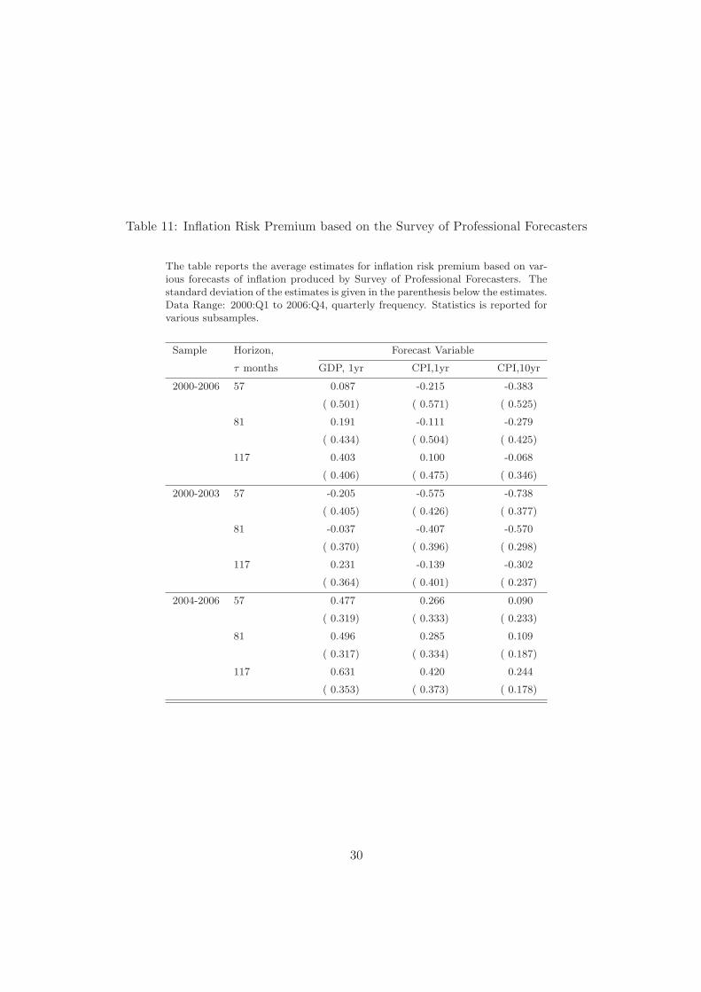
Table 11: Inflation Risk Premium based on the Survey of Professional Forecasters

The table reports the average estimates for inflation risk premium based on var-ious forecasts of inflation produced by Survey of Professional Forecasters. Thestandard deviation of the estimates is given in the parenthesis below the estimates.Data Range: 2000:Q1 to 2006:Q4, quarterly frequency. Statistics is reported forvarious subsamples.

Sample Horizon, Forecast Variable

τ months GDP, 1yr CPI,1yr CPI,10yr

2000-2006 57 0.087 -0.215 -0.383

( 0.501) ( 0.571) ( 0.525)

81 0.191 -0.111 -0.279

( 0.434) ( 0.504) ( 0.425)

117 0.403 0.100 -0.068

( 0.406) ( 0.475) ( 0.346)

2000-2003 57 -0.205 -0.575 -0.738

( 0.405) ( 0.426) ( 0.377)

81 -0.037 -0.407 -0.570

( 0.370) ( 0.396) ( 0.298)

117 0.231 -0.139 -0.302

( 0.364) ( 0.401) ( 0.237)

2004-2006 57 0.477 0.266 0.090

( 0.319) ( 0.333) ( 0.233)

81 0.496 0.285 0.109

( 0.317) ( 0.334) ( 0.187)

117 0.631 0.420 0.244

( 0.353) ( 0.373) ( 0.178)

30

Table 12: Liquidity Risk Premium Regressions

The table reports the estimates of the following regression:

IRPt(τ) = α0 + α1spreadt(τ) + α2volumet(τ) + ut(τ),

where IRPt(τ) is the inflation risk premium computed using expected inflation from theSurvey of Professional Forecasters and τ = 10 years in this table. spreadt(τ) is the averagebid-ask spread (in basis points) of the outstanding 10-year TIPS issues, and volumet(τ) isthe log trading volume averaged across both on-the-run and off-the-run 10-year TIPS. ut(τ)is the residual of the inflation risk premium not explained by liquidity variables. Model Irefers to the regression model where only the bid-ask spread is considered as the explanatoryvariable. Model II refers to the regression model where only the trading volume is consideredas the explanatory variable. Model III refers to the regression model where both the bid-askspread and the trading volume are considered as explanatory variables. The average residualis reported for both the first and the second half of the sample. Spreads data are obtainedfrom Bloomberg and volume data are from Datastream. t−stats are given in parenthesesbelow. Estimation period is 2000:Q1-2006:Q4, the data frequency is quarterly.

Regression α0 α1 α2 R2 Average residual

Models First half Second half

Model I -1.653 29.160 0.335 -0.161 0.161

(-3.747) ( 3.621)

Model II 0.195 0.244 0.283 -0.176 0.176

( 1.958) ( 3.207)

Model III -1.036 20.350 0.128 0.383 -0.141 0.141

(-1.668) ( 2.004) ( 1.385)

31

2000 2001 2002 2003 2004 2005 2006 20072

4

6

8

%

Panel A: Nominal yields

5yr7yr10yr

2000 2001 2002 2003 2004 2005 2006 20070

2

4

6

%

Panel B: TIPS yields

5yr7yr10yr

2000 2001 2002 2003 2004 2005 2006 20071.5

2

2.5

3

time

%

Panel C: TIPS 10−year breakeven rate

Figure 1: Zero-coupon Nominal and TIPS yields of 5, 7, and 10 year maturities fromJanuary 2000 to December 2006, and 10-year TIPS breakeven rate based on zero-couponyield curves.

32

2000 2001 2002 2003 2004 2005 2006 20071.6

1.8

2

2.2

2.4

2.6

2.8

3

3.2

yiel

ds, %

10−year breakeven inflation and 10−year SPF inflation forecast

10−year spreadSPF forecast

Figure 2: The 10-year breakeven inflation rate and the Survey of Professional Forecasters10-year inflation forecast.

33

50 60 70 80 90 100 110 120

020

4060

80100

−0.02

−0.01

0

0.01

tau, horizon

Estimated Inflation Risk Premium based on CPI

time

IRP

50 60 70 80 90 100 110 120

020

4060

80100

−0.02

−0.01

0

0.01

tau, horizon

Estimated Inflation Risk Premium based on Core CPI

time

IRP

Figure 3: This figure presents inflation risk premium based on 5-year expected inflationreported in Table 4. Panel A shows inflation risk premium based on CPI, Consumer PriceIndex for All Urban Consumers, seasonally un-adjusted. Panel B presents inflation riskpremium based on Core CPI, Consumer Price Index Less Food and Energy, seasonallyadjusted. Data range is 2000:01 to 2006:12, monthly frequency.

34