JIP Aversion Modeling Final Report Adam S. Frankel, …gisserver.intertek.com/JIP/DMS/ProjectReports/Cat2/Frankel2016... · JIP Aversion Modeling Final Report Adam S. Frankel, Ph.D

JIPAversionModelingFinalReport

AdamS.Frankel,Ph.D.WilliamT.Ellison,Ph.D.AndrewW.White,Ph.D.

KathleenJ.Vigness‐Raposa,Ph.D.

MarineAcoustics,Inc.

MAI947

31July2016

TN16–015

2

Table of Contents

INTRODUCTION......................................................................................................................................................3

METHODS.................................................................................................................................................................4SOURCEANDPROPAGATIONMODELING.............................................................................................................................4ANIMATMODELING................................................................................................................................................................7MODELEDANIMALTYPES.....................................................................................................................................................9EVALUATIONOFMODELINGRESULTS...............................................................................................................................14

RESULTS.................................................................................................................................................................15SOURCECHARACTERISTICS.................................................................................................................................................15ACOUSTICSOUNDFIELDS(TLSLICES).............................................................................................................................16EXPOSURERESULTS..............................................................................................................................................................18

LITERATURECITED...........................................................................................................................................39

APPENDIXI:NUMBERSOFANIMALSEXPOSEDTOSOUNDLEVELSEXCEEDINGCRITERIATHRESHOLDS.......................................................................................................................................................41

3

Introduction MarineAcoustics,Inc.(MAI)modeledaseismicarrayanditsunderwateracoustic

propagationduringexemplarone‐monthexplorationsurveysintheGulfofMexicotoexaminemarinemammalexposureestimatesoveraselectedcombinationofsourceandanimalmovementparameters.Fourselectedmarinemammaltypes,representingonelow(LF),twomid(MF)andonehigh(HF)frequencymembersofthehearinggroupsdefinedbySouthalletal.(2007),aswellastwosurveyconfigurations,representingnominal2Dand3Dairgunarraysurveys,aswellasastationarysourcesurvey,wereevaluatedinthisparametricstudy.TheacousticexposureandanimalresponsewereestimatedusingtheAcousticIntegrationModel©

(AIM).Foursource/animalsimulationcaseswereundertaken:

(1)stationarysourcewithstationarybutdivinganimals,(2)movingsourcewithstationarybutdivinganimals,(3)movingsourcewithmovinganddivinganimals,and(4)movingsourcewithmovinganddivinganimalswithaversivebehaviorstoreceivedsoundpressurelevels(SPL).Thesemovementswereconvolvedwiththeoutputofthesourceacousticpropagationmodeltocalculatethefull30‐dayexposurehistoriesforeachsimulatedanimalforeachsurveyconfiguration.Theseresultswerefrequencyweightedusingnoweighting,M‐weighting(Southalletal.,2007),NavyTypeIIweighting(FinneranandJenkins,2012)andproposedNOAAguidance(NOAA,2016).Theresultant30‐dayexposurehistoriesforeachanimalwereevaluatedusingbothtraditionalmetrics(unweighted160dBSPLforbehavior,180dBSPLforinjury)aswellasavarietyofTTSandPTSthresholdsfromSouthalletal.(2007),FinneranandJenkins(2012)andNOAA(2016).

ThisstudysignificantlyparallelsthemodelingassessmentpresentedinEllisonetal.(2016).Thatstudyprovidesdiscussionandevaluationtechniquesthatarecomplementarytothisreport,particularlywithregardtotheevaluationofproportionally‐scaledaversionofanimalstoreceivedsoundpressurelevels.InEllisonetal.(2016),thefull2008fallbowheadmigration(ca.10,000animals)wereindividuallyassessedduringa47‐dayperiodcoveringthepopulation’swestwardmigrationpastasimulationofnineselectedindustrynoisesourcesthatwereoperatinginthatareaandtime.ThenominalpassagetimeintheEllisonetal.(2016)studywasapproximatelyoneweekforanindividualanimal.Theunderlyingobjectiveinbothofthesestudieswastomodeleachindividualanimal(animat)continuouslyfortheentireperiodofpotentialexposure,witha‘dosimeter’recordingofexposurehistory.

4

Methods

Source and Propagation Modeling

Acoustic Source Model

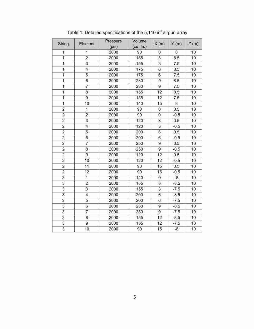
ThecurrentstudyusedacombinationofmethodstoevaluatethesourcecharacteristicsoftheairgunarraydescribedinTable1.ThefirststepwastoinputafulldescriptionoftheairgunintotheGundalfmodel(Hatton,2008)thatpredictedthearraysourcespectrumusedtocalculatethe1/3‐octaveSELsourcelevelsforthearrayfrom10Hzto1kHz.

ThedirectivitypatternofthearraywascalculatedusingthevolumetricbeampatterngeneratormoduleintheCASS‐GRABpackage(Burdic,1984;Weinberg,2004).Theinputstothemodulewerethex,y,andzlocationofeachgunandtherelativeamplitudeofeachgun,representedasthecuberootofitsvolume.Thedirectivitypatternwasgeneratedforeverytwodegreesofdeclination(verticaldirection)from+90to‐90,every10degreesinazimuth(horizontaldirection)andforeach1/3‐octavebandcenterfrequencyfrom10Hzto1kHz.

Acoustic Propagation Modeling

Thesoundfieldcreatedbytheproposedairgunarraywasmodeledusingtherange‐dependentacousticmodel(RAM).RAMisaPE‐basedmodelthatincorporatesageoacousticoceanbottommodelthataccountsforbottomlossduetoshearwavepropagation(Collins,1993).

Physical Environmental Inputs

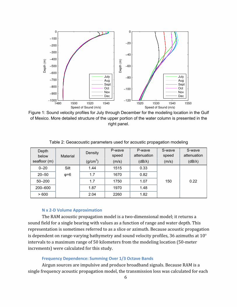
TheOAMLGeneralizedDigitalEnvironmentalModel(GDEM)Version3.0database(NavalOceanographicOffice,2003)wasaccessedforsoundvelocityprofiles.ThesoundvelocityprofilesforJulythroughDecemberareshownbelow(Figure1).TheOctoberprofileswereusedforpropagationmodeling.

GeoacousticmodelparameterswereextractedfromtheGulfofMexicoG&GActivitiesDraftProgrammaticEIS,AppendixD,Table53(Zeddiesetal.,2015).TheseareshowninTable2.

5

Table 1: Detailed specifications of the 5,110 in3 airgun array

String Element Pressure

(psi) Volume (cu. In.)

X (m) Y (m) Z (m)

1 1 2000 90 0 8 10 1 2 2000 155 3 8.5 10 1 3 2000 155 3 7.5 10 1 4 2000 175 6 8.5 10 1 5 2000 175 6 7.5 10 1 6 2000 230 9 8.5 10 1 7 2000 230 9 7.5 10 1 8 2000 155 12 8.5 10 1 9 2000 155 12 7.5 10 1 10 2000 140 15 8 10 2 1 2000 90 0 0.5 10 2 2 2000 90 0 -0.5 10 2 3 2000 120 3 0.5 10 2 4 2000 120 3 -0.5 10 2 5 2000 200 6 0.5 10 2 6 2000 200 6 -0.5 10 2 7 2000 250 9 0.5 10 2 8 2000 250 9 -0.5 10 2 9 2000 120 12 0.5 10 2 10 2000 120 12 -0.5 10 2 11 2000 90 15 0.5 10 2 12 2000 90 15 -0.5 10 3 1 2000 140 0 -8 10 3 2 2000 155 3 -8.5 10 3 3 2000 155 3 -7.5 10 3 4 2000 200 6 -8.5 10 3 5 2000 200 6 -7.5 10 3 6 2000 230 9 -8.5 10 3 7 2000 230 9 -7.5 10 3 8 2000 155 12 -8.5 10 3 9 2000 155 12 -7.5 10 3 10 2000 90 15 -8 10

6

Figure 1: Sound velocity profiles for July through December for the modeling location in the Gulf of Mexico. More detailed structure of the upper portion of the water column is presented in the

right panel.

Table 2: Geoacoustic parameters used for acoustic propagation modeling

Depth below

seafloor (m) Material

Density P-wave speed

P-wave attenuation

S-wave speed

S-wave attenuation

(g/cm3) (m/s) (dB/λ) (m/s) (dB/λ)

0–20 Silt 1.44 1515 0.33

150 0.22

20–50 φ=6 1.7 1670 0.82

50–200 1.7 1750 1.07

200–600 1.87 1970 1.48

> 600 2.04 2260 1.82

N x 2‐D Volume Approximation

TheRAMacousticpropagationmodelisatwo‐dimensionalmodel;itreturnsasoundfieldforasinglebearingwithvaluesasafunctionofrangeandwaterdepth.Thisrepresentationissometimesreferredtoasasliceorazimuth.Becauseacousticpropagationisdependentonrange‐varyingbathymetryandsoundvelocityprofiles,36azimuthsat10intervalstoamaximumrangeof50kilometersfromthemodelinglocation(50‐meterincrements)werecalculatedforthisstudy.

Frequency Dependence: Summing Over 1/3 Octave Bands

Airgunsourcesareimpulsiveandproducebroadbandsignals.BecauseRAMisasinglefrequencyacousticpropagationmodel,thetransmissionlosswascalculatedforeach

7

1/3‐octavebandcenterfrequencyfrom10Hzto1kHz.Eachtransmissionlossslicewassubtractedfromitscorrespondingsourcelevelvaluetoproduceasliceofreceivedsoundexposurelevels.Theseseparate1/3‐octavebandsoundlevelfieldswerethencombinedasintensitiestoproduceabroadband,three‐dimensionalacousticfieldforthemodelinglocation.Thisprocesswasrepeatedwithsourcelevelvaluesthathadbeenadjustedwithauditoryweightingfunctions,sothatthefinaloutputincludedmultipleSELacousticfields:a‘flat’orunweightedacousticfield,aswellasnineweightedacousticfieldsthatincorporatedtheM‐weighting,NavyTypeIIandNOAA(2016)auditoryweightingfunctionsforlow‐,mid‐,andhigh‐frequencycetaceans.

ThesourcelevelcalculatedfromthearraysignatureisaSoundExposureLevel(SEL)measure.However,RMSvaluesarealsoneededforbehavioralresponseevaluation.TheformulasdescribedintheFinalProgrammaticEnvironmentalImpactStatement(EIS)fortheAtlanticOuterContinentalShelfProposedGeologicalandGeophysicalActivities:Mid‐AtlanticandSouthAtlanticPlanningAreas(http://www.boem.gov/Atlantic‐G‐G‐PEIS/#Final%20PEIS)wereappliedtotheSELversionsoftheacousticfieldstocreatetheirRMSpressureequivalents.

Animat Modeling

TheAcousticIntegrationModel©(AIM)isanindividual‐based,MonteCarlostatisticalmodeldesignedtopredicttheexposureofreceiverstoanystimuluspropagatingthroughspaceandtime,whichinthisanalysisisacousticenergy(Frankeletal.,2002).ThecentralcomponentofAIMistheanimatmovementengine,whereparameterscontrolthespeedanddirectionofmovementof“animats”inthree‐dimensionalspaceatspecifiedtimeintervalstocreateafullfour‐dimensionalsimulationoftheproposedsurvey.AIMhasbeenusedformanyenvironmentalcompliancedocumentsandwasapprovedbyexternalCenterforIndependentExperts(CIE)review(Cordue,2006).

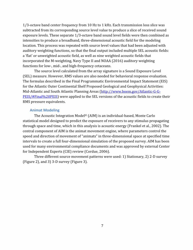
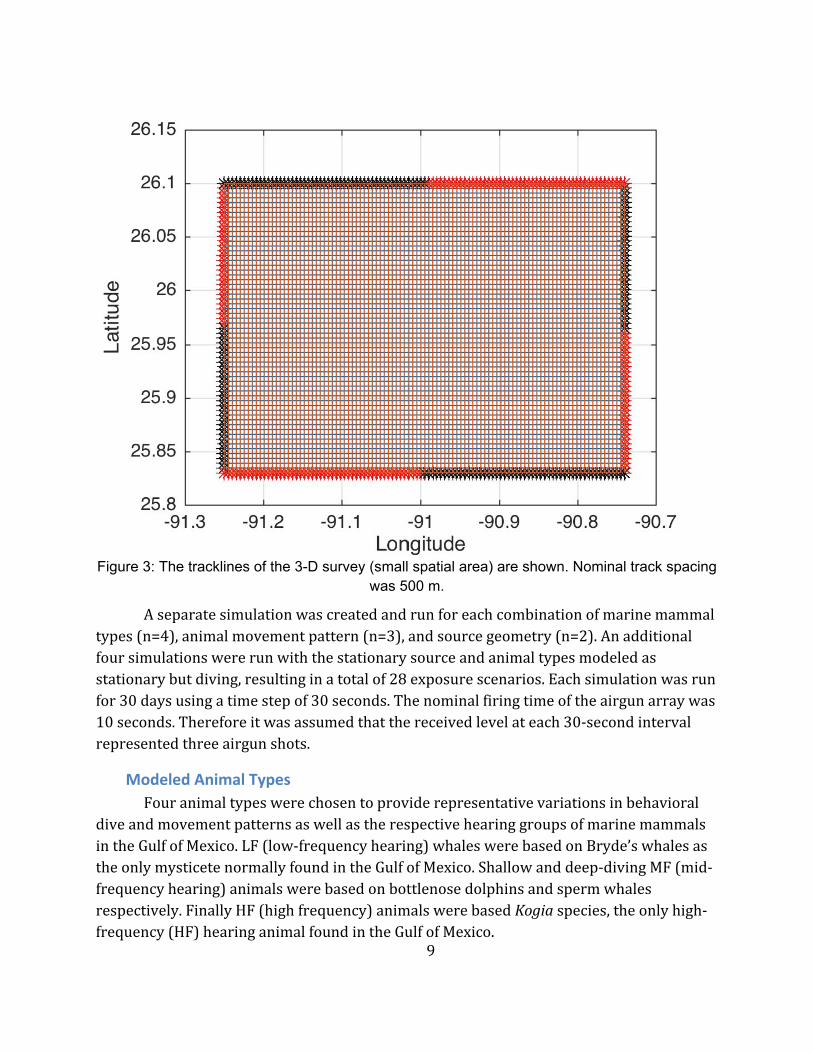
Threedifferentsourcemovementpatternswereused:1)Stationary,2)2‐Dsurvey(Figure2),and3)3‐Dsurvey(Figure3).

8

Figure 2: The track lines of the 2-D survey (large spatial area) are shown. Nominal spacing

between tracks was 10 km.

9

Figure 3: The tracklines of the 3-D survey (small spatial area) are shown. Nominal track spacing

was 500 m.

Aseparatesimulationwascreatedandrunforeachcombinationofmarinemammaltypes(n=4),animalmovementpattern(n=3),andsourcegeometry(n=2).Anadditionalfoursimulationswererunwiththestationarysourceandanimaltypesmodeledasstationarybutdiving,resultinginatotalof28exposurescenarios.Eachsimulationwasrunfor30daysusingatimestepof30seconds.Thenominalfiringtimeoftheairgunarraywas10seconds.Thereforeitwasassumedthatthereceivedlevelateach30‐secondintervalrepresentedthreeairgunshots.

Modeled Animal Types

FouranimaltypeswerechosentoproviderepresentativevariationsinbehavioraldiveandmovementpatternsaswellastherespectivehearinggroupsofmarinemammalsintheGulfofMexico.LF(low‐frequencyhearing)whaleswerebasedonBryde’swhalesastheonlymysticetenormallyfoundintheGulfofMexico.Shallowanddeep‐divingMF(mid‐frequencyhearing)animalswerebasedonbottlenosedolphinsandspermwhalesrespectively.FinallyHF(highfrequency)animalswerebasedKogiaspecies,theonlyhigh‐frequency(HF)hearinganimalfoundintheGulfofMexico.

10

Animal movement cases:

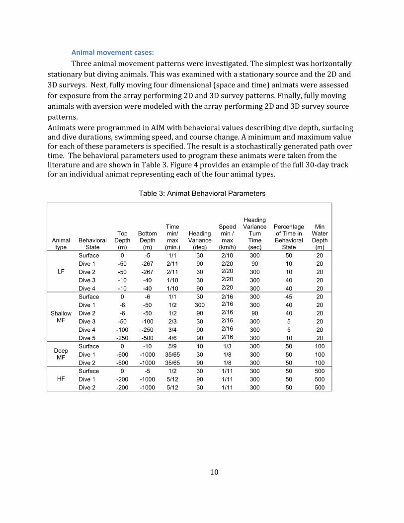
Threeanimalmovementpatternswereinvestigated.Thesimplestwashorizontallystationarybutdivinganimals.Thiswasexaminedwithastationarysourceandthe2Dand3Dsurveys.Next,fullymovingfourdimensional(spaceandtime)animatswereassessedforexposurefromthearrayperforming2Dand3Dsurveypatterns.Finally,fullymovinganimalswithaversionweremodeledwiththearrayperforming2Dand3Dsurveysourcepatterns.AnimatswereprogrammedinAIMwithbehavioralvaluesdescribingdivedepth,surfacinganddivedurations,swimmingspeed,andcoursechange.Aminimumandmaximumvalueforeachoftheseparametersisspecified.Theresultisastochasticallygeneratedpathovertime.ThebehavioralparametersusedtoprogramtheseanimatsweretakenfromtheliteratureandareshowninTable3.Figure4providesanexampleofthefull30‐daytrackforanindividualanimatrepresentingeachofthefouranimaltypes.

Table 3: Animat Behavioral Parameters

Animal type

Behavioral State

Top Depth

(m)

Bottom Depth

(m)

Time min/ max

(min.)

Heading Variance

(deg)

Speed min / max

(km/h)

Heading Variance

Turn Time (sec)

Percentage of Time in Behavioral

State

Min Water Depth

(m)

LF

Surface 0 -5 1/1 30 2/10 300 50 20 Dive 1 -50 -267 2/11 90 2/20 90 10 20 Dive 2 -50 -267 2/11 30 2/20 300 10 20 Dive 3 -10 -40 1/10 30 2/20 300 40 20 Dive 4 -10 -40 1/10 90 2/20 300 40 20

Shallow MF

Surface 0 -6 1/1 30 2/16 300 45 20 Dive 1 -6 -50 1/2 300 2/16 300 40 20 Dive 2 -6 -50 1/2 90 2/16 90 40 20 Dive 3 -50 -100 2/3 30 2/16 300 5 20 Dive 4 -100 -250 3/4 90 2/16 300 5 20 Dive 5 -250 -500 4/6 90 2/16 300 10 20

Deep MF

Surface 0 -10 5/9 10 1/3 300 50 100 Dive 1 -600 -1000 35/65 30 1/8 300 50 100 Dive 2 -600 -1000 35/65 90 1/8 300 50 100

HF Surface 0 -5 1/2 30 1/11 300 50 500 Dive 1 -200 -1000 5/12 90 1/11 300 50 500 Dive 2 -200 -1000 5/12 30 1/11 300 50 500

11

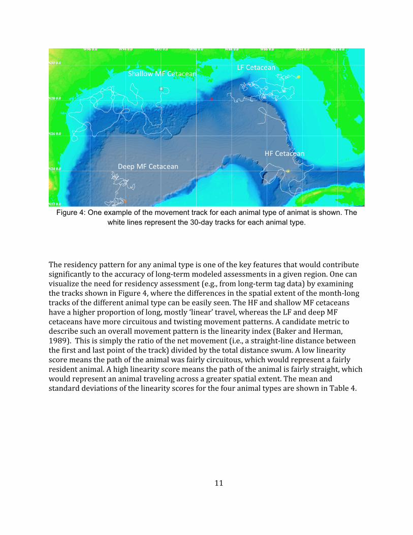
Figure 4: One example of the movement track for each animal type of animat is shown. The

white lines represent the 30-day tracks for each animal type.

Theresidencypatternforanyanimaltypeisoneofthekeyfeaturesthatwouldcontributesignificantlytotheaccuracyoflong‐termmodeledassessmentsinagivenregion.Onecanvisualizetheneedforresidencyassessment(e.g.,fromlong‐termtagdata)byexaminingthetracksshowninFigure4,wherethedifferencesinthespatialextentofthemonth‐longtracksofthedifferentanimaltypecanbeeasilyseen.TheHFandshallowMFcetaceanshaveahigherproportionoflong,mostly‘linear’travel,whereastheLFanddeepMFcetaceanshavemorecircuitousandtwistingmovementpatterns.Acandidatemetrictodescribesuchanoverallmovementpatternisthelinearityindex(BakerandHerman,1989).Thisissimplytheratioofthenetmovement(i.e.,astraight‐linedistancebetweenthefirstandlastpointofthetrack)dividedbythetotaldistanceswum.Alowlinearityscoremeansthepathoftheanimalwasfairlycircuitous,whichwouldrepresentafairlyresidentanimal.Ahighlinearityscoremeansthepathoftheanimalisfairlystraight,whichwouldrepresentananimaltravelingacrossagreaterspatialextent.ThemeanandstandarddeviationsofthelinearityscoresforthefouranimaltypesareshowninTable4.

12

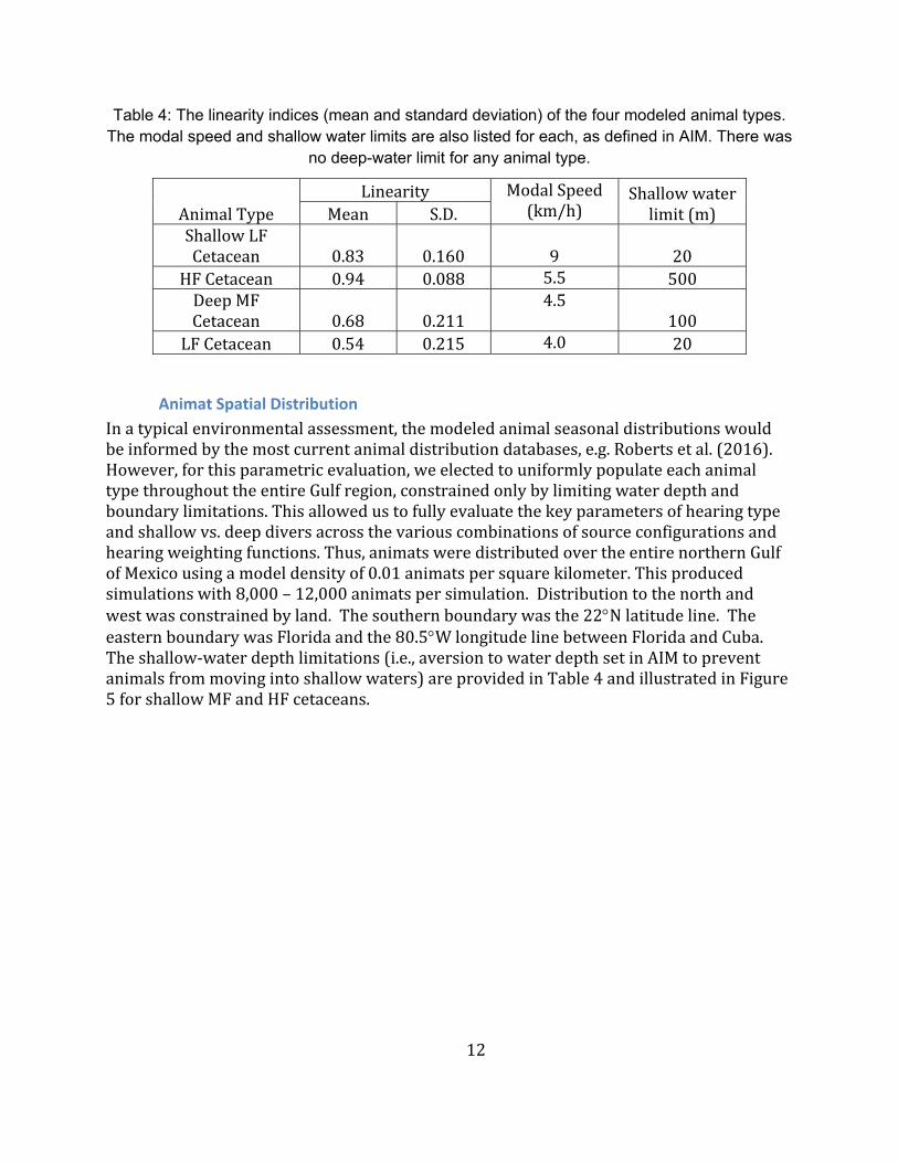
Table 4: The linearity indices (mean and standard deviation) of the four modeled animal types. The modal speed and shallow water limits are also listed for each, as defined in AIM. There was

no deep-water limit for any animal type.

AnimalTypeLinearity ModalSpeed

(km/h)Shallowwaterlimit(m)Mean S.D.

ShallowLFCetacean 0.83 0.160 9 20

HFCetacean 0.94 0.088 5.5 500DeepMFCetacean 0.68 0.211

4.5100

LFCetacean 0.54 0.215 4.0 20

Animat Spatial Distribution

Inatypicalenvironmentalassessment,themodeledanimalseasonaldistributionswouldbeinformedbythemostcurrentanimaldistributiondatabases,e.g.Robertsetal.(2016).However,forthisparametricevaluation,weelectedtouniformlypopulateeachanimaltypethroughouttheentireGulfregion,constrainedonlybylimitingwaterdepthandboundarylimitations.Thisallowedustofullyevaluatethekeyparametersofhearingtypeandshallowvs.deepdiversacrossthevariouscombinationsofsourceconfigurationsandhearingweightingfunctions.Thus,animatsweredistributedovertheentirenorthernGulfofMexicousingamodeldensityof0.01animatspersquarekilometer.Thisproducedsimulationswith8,000–12,000animatspersimulation.Distributiontothenorthandwestwasconstrainedbyland.Thesouthernboundarywasthe22Nlatitudeline.TheeasternboundarywasFloridaandthe80.5WlongitudelinebetweenFloridaandCuba.Theshallow‐waterdepthlimitations(i.e.,aversiontowaterdepthsetinAIMtopreventanimalsfrommovingintoshallowwaters)areprovidedinTable4andillustratedinFigure5forshallowMFandHFcetaceans.

13

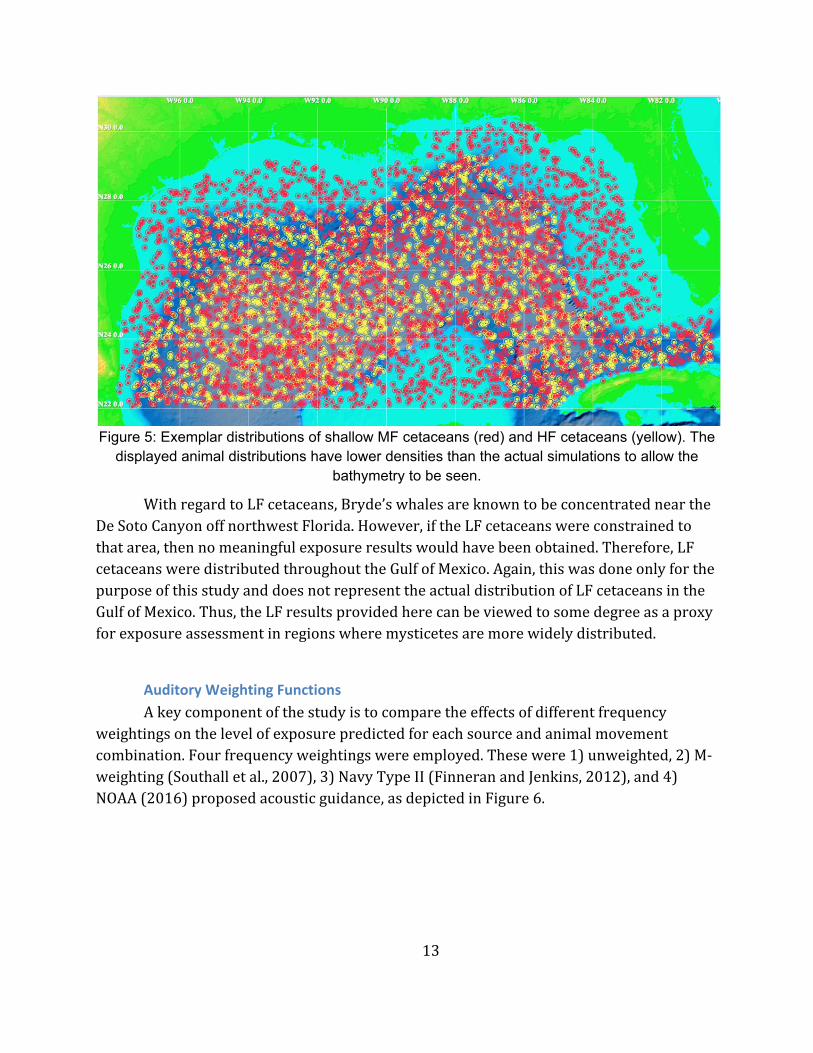
Figure 5: Exemplar distributions of shallow MF cetaceans (red) and HF cetaceans (yellow). The

displayed animal distributions have lower densities than the actual simulations to allow the bathymetry to be seen.

WithregardtoLFcetaceans,Bryde’swhalesareknowntobeconcentratedneartheDeSotoCanyonoffnorthwestFlorida.However,iftheLFcetaceanswereconstrainedtothatarea,thennomeaningfulexposureresultswouldhavebeenobtained.Therefore,LFcetaceansweredistributedthroughouttheGulfofMexico.Again,thiswasdoneonlyforthepurposeofthisstudyanddoesnotrepresenttheactualdistributionofLFcetaceansintheGulfofMexico.Thus,theLFresultsprovidedherecanbeviewedtosomedegreeasaproxyforexposureassessmentinregionswheremysticetesaremorewidelydistributed.

Auditory Weighting Functions

Akeycomponentofthestudyistocomparetheeffectsofdifferentfrequencyweightingsonthelevelofexposurepredictedforeachsourceandanimalmovementcombination.Fourfrequencyweightingswereemployed.Thesewere1)unweighted,2)M‐weighting(Southalletal.,2007),3)NavyTypeII(FinneranandJenkins,2012),and4)NOAA(2016)proposedacousticguidance,asdepictedinFigure6.

14

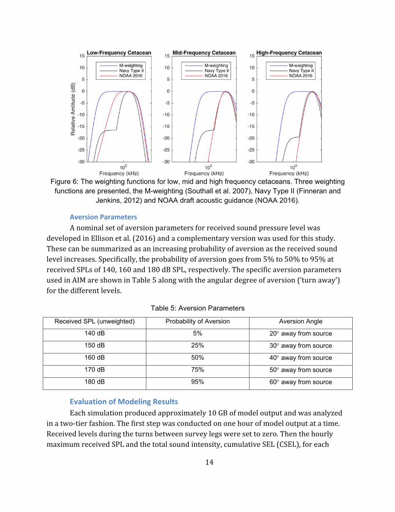
Figure 6: The weighting functions for low, mid and high frequency cetaceans. Three weighting

functions are presented, the M-weighting (Southall et al. 2007), Navy Type II (Finneran and Jenkins, 2012) and NOAA draft acoustic guidance (NOAA 2016).

Aversion Parameters

AnominalsetofaversionparametersforreceivedsoundpressurelevelwasdevelopedinEllisonetal.(2016)andacomplementaryversionwasusedforthisstudy.Thesecanbesummarizedasanincreasingprobabilityofaversionasthereceivedsoundlevelincreases.Specifically,theprobabilityofaversiongoesfrom5%to50%to95%atreceivedSPLsof140,160and180dBSPL,respectively.ThespecificaversionparametersusedinAIMareshowninTable5alongwiththeangulardegreeofaversion(‘turnaway’)forthedifferentlevels.

Table 5: Aversion Parameters

Received SPL (unweighted) Probability of Aversion Aversion Angle

140 dB 5% 20 away from source





Evaluation of Modeling Results

Eachsimulationproducedapproximately10GBofmodeloutputandwasanalyzedinatwo‐tierfashion.Thefirststepwasconductedononehourofmodeloutputatatime.Receivedlevelsduringtheturnsbetweensurveylegsweresettozero.ThenthehourlymaximumreceivedSPLandthetotalsoundintensity,cumulativeSEL(CSEL),foreach

15

animatwascalculatedandstoredinasummaryfile.Thisreducedthenumberofobservationsfrom86,400to720rows.

Thesehourlymetricswerethenusedtocreatethemaximumunweightedreceivedsoundpressurelevel(MSPL)foreach24‐hrperiodofthe30‐daysurveydurationmodeledforeachanimat.Likewise,cumulativeSELmetricswerealsocalculatedforeach24‐hrperiodofthe30‐daysurveydurationmodeledforeachanimat.ThiscalculationincludedtheSELcorrection(added5dB)neededtoaccountforthethreeairgunarrayshotsthatoccurredduringeach30secondmodelstep.MeanMSPLandCSELvalueswerethencalculatedforeachanimat.Thesewerecomparedtothe160/180dBSPLcriteriafortraditionalLevelBandLevelAexposuresaswellastheSELcriteriaforTTSandPTSinSouthalletal.(2007),FinneranandJenkins(2012)andNOAA(2016).Southalletal.(2007)onlyproposedacriterionforPTS.ATTScriterionforM‐weightingwascreatedbysubtracting20dBfromthePTScriterion.TheSouthalletal.(2007)criteriawerealsousedfortheunweightedCSELmetrics,asnopreviouscriteriaexisted.Themeannumberofdailyexposuresthatexceededthosecriteria(i.e.,takes)resultedfromthisapproach.

Asstated,thisstudyisfocusedontheeffectsofsurveydesignandanimalbehaviorpatternsonexposureestimatesandnotassessingactualenvironmentalimpact.Thereforenocorrectionwasmadetoscalethemodeledanimaldensitiestolocalanimaldensities,asthiswouldonlyaddconfusionandanadditionalsourceofuncertainty.

Results

Source Characteristics

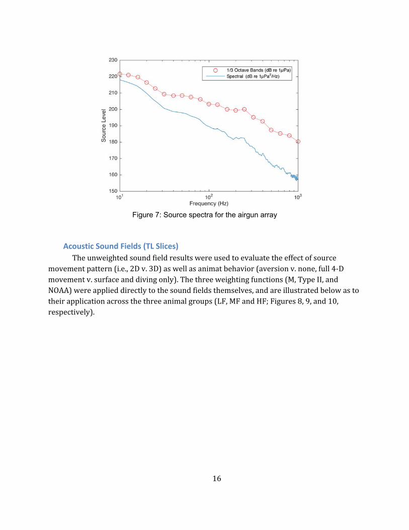
TheGundalfmodelwasusedtopredictthesourcelevelandspectrumoftheairgunarray.TheresultingsourcespectraareshowninFigure7.Bothspectraland1/3‐octavebandvaluesarepresented.Thesearethe‘unghosted’versionsofthespectrum,asthepropagationmodelexplicitlyconsiderstheeffectofsurfacereflection.

16

Figure 7: Source spectra for the airgun array

Acoustic Sound Fields (TL Slices)

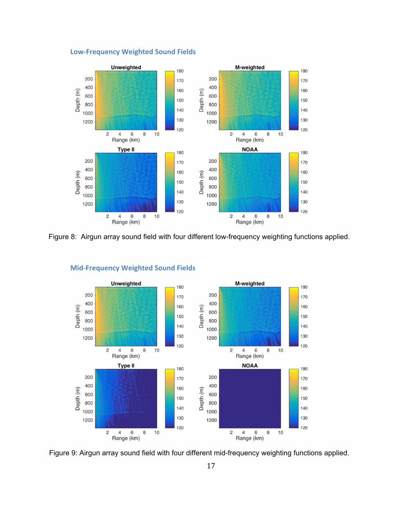
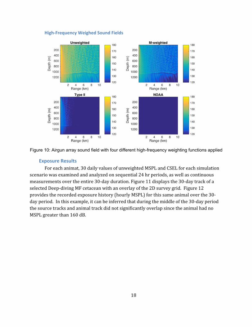
Theunweightedsoundfieldresultswereusedtoevaluatetheeffectofsourcemovementpattern(i.e.,2Dv.3D)aswellasanimatbehavior(aversionv.none,full4‐Dmovementv.surfaceanddivingonly).Thethreeweightingfunctions(M,TypeII,andNOAA)wereapplieddirectlytothesoundfieldsthemselves,andareillustratedbelowastotheirapplicationacrossthethreeanimalgroups(LF,MFandHF;Figures8,9,and10,respectively).

17

Low‐Frequency Weighted Sound Fields

Figure 8: Airgun array sound field with four different low-frequency weighting functions applied.

Mid‐Frequency Weighted Sound Fields

Figure 9: Airgun array sound field with four different mid-frequency weighting functions applied.

18

High‐Frequency Weighed Sound Fields

Figure 10: Airgun array sound field with four different high-frequency weighting functions applied

Exposure Results

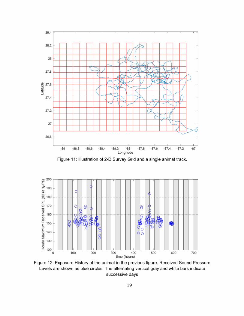
Foreachanimat,30dailyvaluesofunweightedMSPLandCSELforeachsimulationscenariowasexaminedandanalyzedonsequential24hrperiods,aswellascontinuousmeasurementsovertheentire30‐dayduration.Figure11displaysthe30‐daytrackofaselectedDeep‐divingMFcetaceanwithanoverlayofthe2Dsurveygrid.Figure12providestherecordedexposurehistory(hourlyMSPL)forthissameanimaloverthe30‐dayperiod.Inthisexample,itcanbeinferredthatduringthemiddleofthe30‐dayperiodthesourcetracksandanimaltrackdidnotsignificantlyoverlapsincetheanimalhadnoMSPLgreaterthan160dB.

19

Figure 11: Illustration of 2-D Survey Grid and a single animat track.

Figure 12: Exposure History of the animat in the previous figure. Received Sound Pressure

Levels are shown as blue circles. The alternating vertical gray and white bars indicate successive days

20

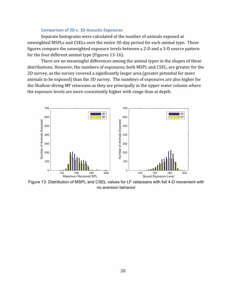
Comparison of 2D v. 3D Acoustic Exposures

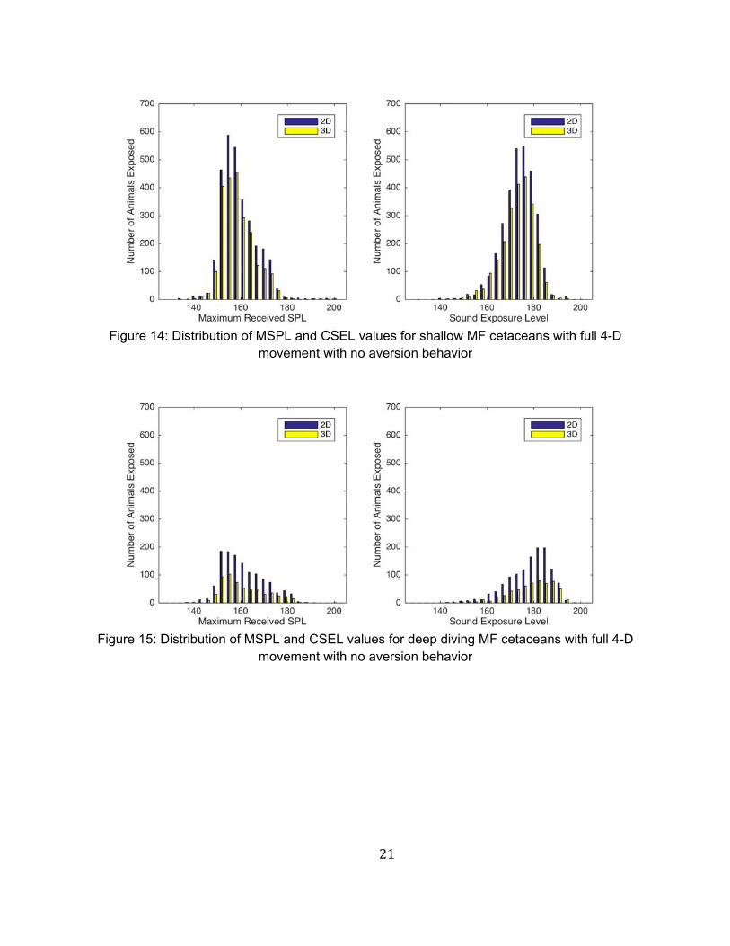
SeparatehistogramswerecalculatedofthenumberofanimalsexposedatunweightedMSPLsandCSELsovertheentire30‐dayperiodforeachanimaltype.Thesefigurescomparetheunweightedexposurelevelsbetweena2‐Danda3‐Dsourcepatternforthefourdifferentanimaltype(Figures13‐16).

Therearenomeaningfuldifferencesamongtheanimaltypesintheshapesofthesedistributions.However,thenumbersofexposures,bothMSPLandCSEL,aregreaterforthe2Dsurvey,asthesurveycoveredasignificantlylargerarea(greaterpotentialformoreanimalstobeexposed)thanthe3Dsurvey.ThenumbersofexposuresarealsohigherfortheShallow‐divingMFcetaceansastheyareprincipallyintheupperwatercolumnwheretheexposurelevelsaremoreconsistentlyhigherwithrangethanatdepth.

Figure 13: Distribution of MSPL and CSEL values for LF cetaceans with full 4-D movement with

no aversion behavior

21

Figure 14: Distribution of MSPL and CSEL values for shallow MF cetaceans with full 4-D

movement with no aversion behavior

Figure 15: Distribution of MSPL and CSEL values for deep diving MF cetaceans with full 4-D

movement with no aversion behavior

22

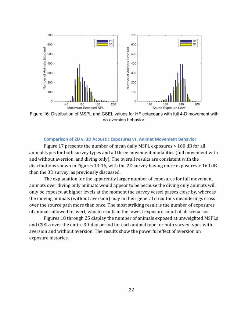
Figure 16: Distribution of MSPL and CSEL values for HF cetaceans with full 4-D movement with

no aversion behavior.

Comparison of 2D v. 3D Acoustic Exposures vs. Animat Movement Behavior

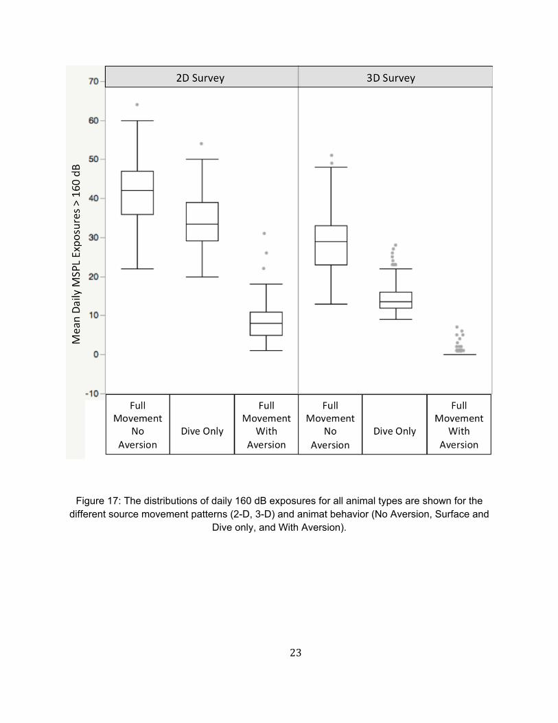
Figure17presentsthenumberofmeandailyMSPLexposures>160dBforallanimaltypesforbothsurveytypesandallthreemovementmodalities(fullmovementwithandwithoutaversion,anddivingonly).TheoverallresultsareconsistentwiththedistributionsshowninFigures13‐16,withthe2Dsurveyhavingmoreexposures>160dBthanthe3Dsurvey,aspreviouslydiscussed.

Theexplanationfortheapparentlylargernumberofexposuresforfullmovementanimatsoverdivingonlyanimatswouldappeartobebecausethedivingonlyanimatswillonlybeexposedathigherlevelsatthemomentthesurveyvesselpassescloseby,whereasthemovinganimals(withoutaversion)mayintheirgeneralcircuitousmeanderingscrossoverthesourcepathmorethanonce.Themoststrikingresultisthenumberofexposuresofanimalsallowedtoavert,whichresultsinthelowestexposurecountofallscenarios.

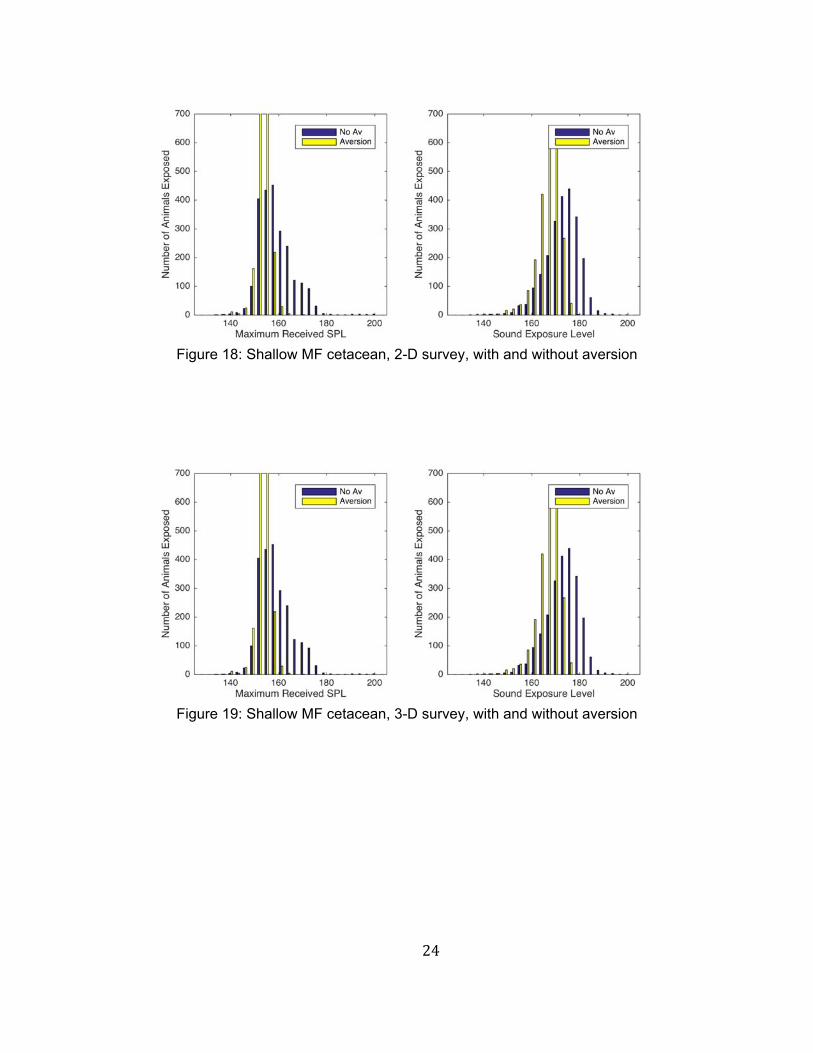
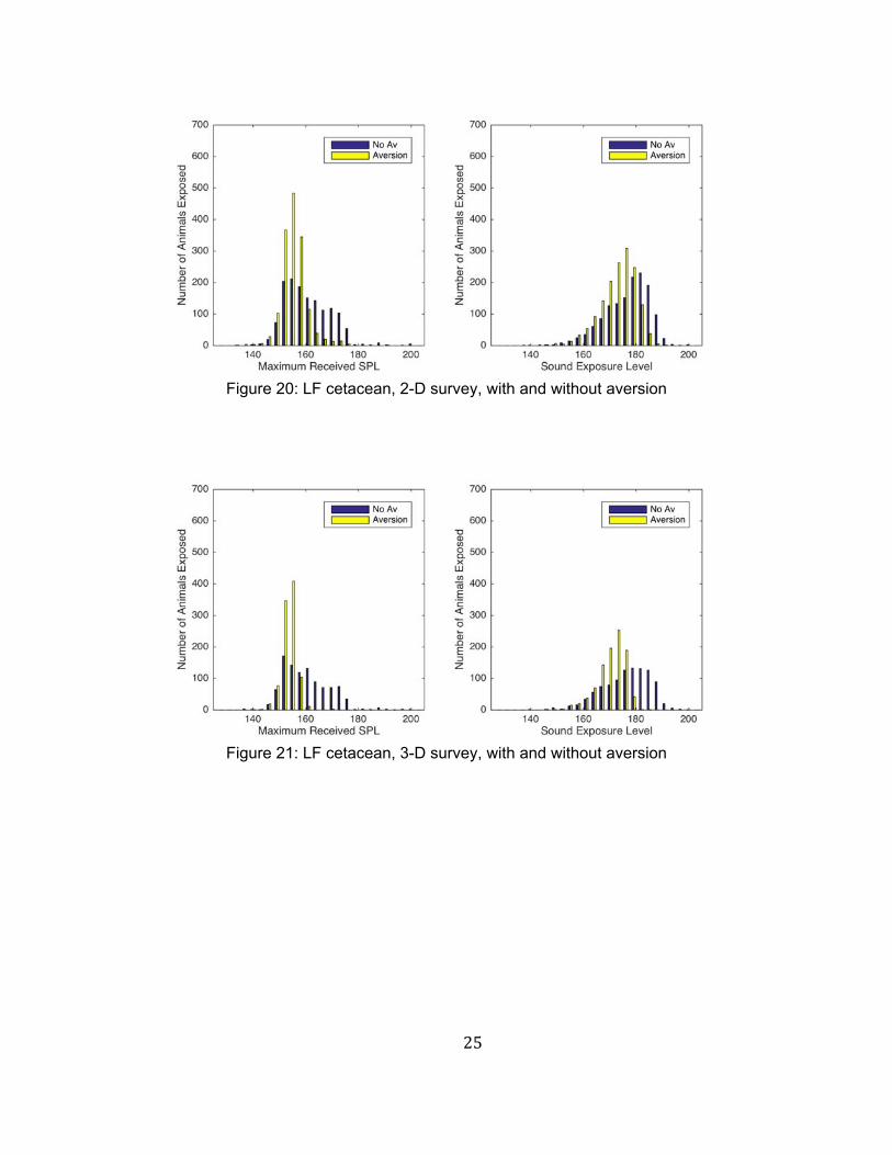
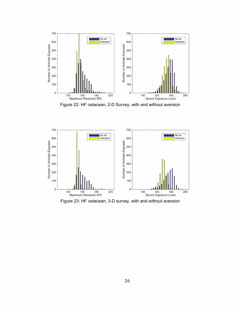
Figures18through25displaythenumberofanimalsexposedatunweightedMSPLsandCSELsovertheentire30‐dayperiodforeachanimaltypeforbothsurveytypeswithaversionandwithoutaversion.Theresultsshowthepowerfuleffectofaversiononexposurehistories.

23

Figure 17: The distributions of daily 160 dB exposures for all animal types are shown for the

different source movement patterns (2-D, 3-D) and animat behavior (No Aversion, Surface and Dive only, and With Aversion).

24

Figure 18: Shallow MF cetacean, 2-D survey, with and without aversion

Figure 19: Shallow MF cetacean, 3-D survey, with and without aversion

25

Figure 20: LF cetacean, 2-D survey, with and without aversion

Figure 21: LF cetacean, 3-D survey, with and without aversion

26

Figure 22: HF cetacean, 2-D Survey, with and without aversion

Figure 23: HF cetacean, 3-D survey, with and without aversion

27

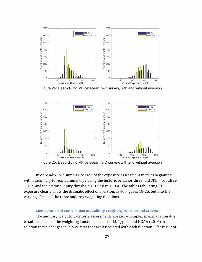
Figure 24: Deep-diving MF cetacean, 2-D survey, with and without aversion

Figure 25: Deep-diving MF cetacean, 3-D survey, with and without aversion

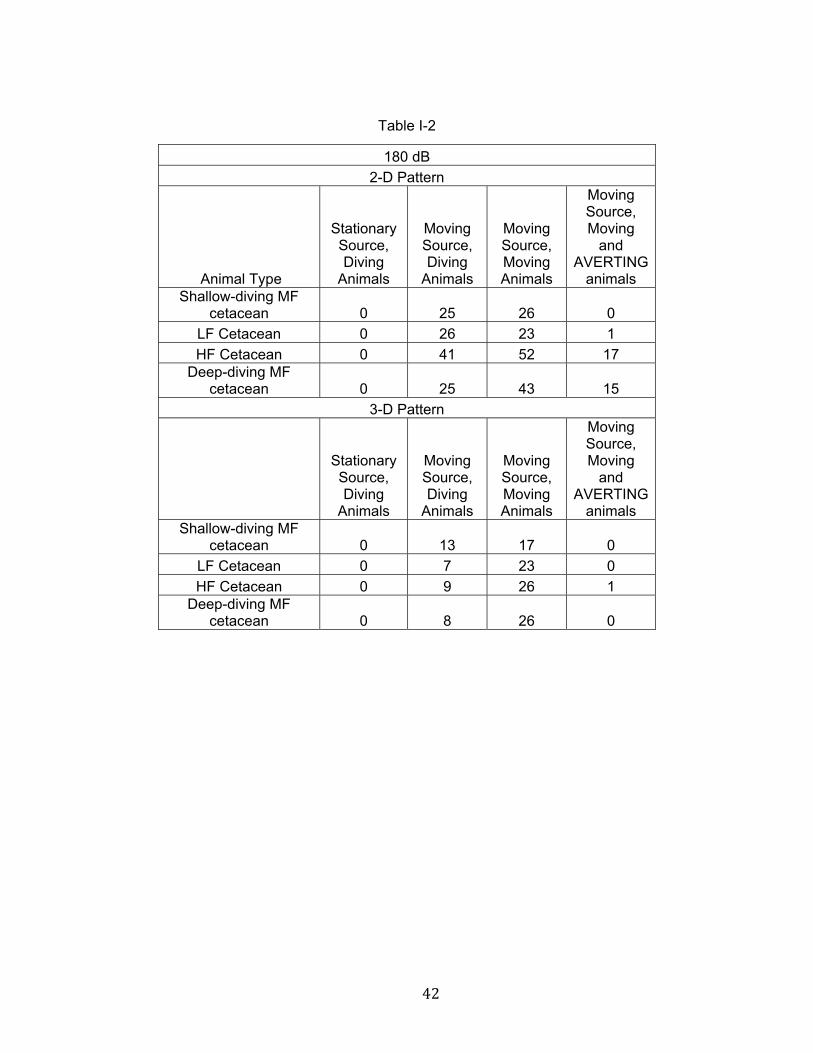
InAppendixIwesummarizeeachoftheexposureassessmentmetricsbeginning

withasummaryforeachanimaltypeusingthehistoricbehaviorthresholdSPL>160dBre1Pa,andthehistoricinjurythreshold>180dBre1Pa.ThetablestabulatingPTSexposureclearlyshowthedramaticeffectofaversion,asdoFigures18‐25,butalsothevaryingeffectsofthethreeauditoryweightingfunctions.

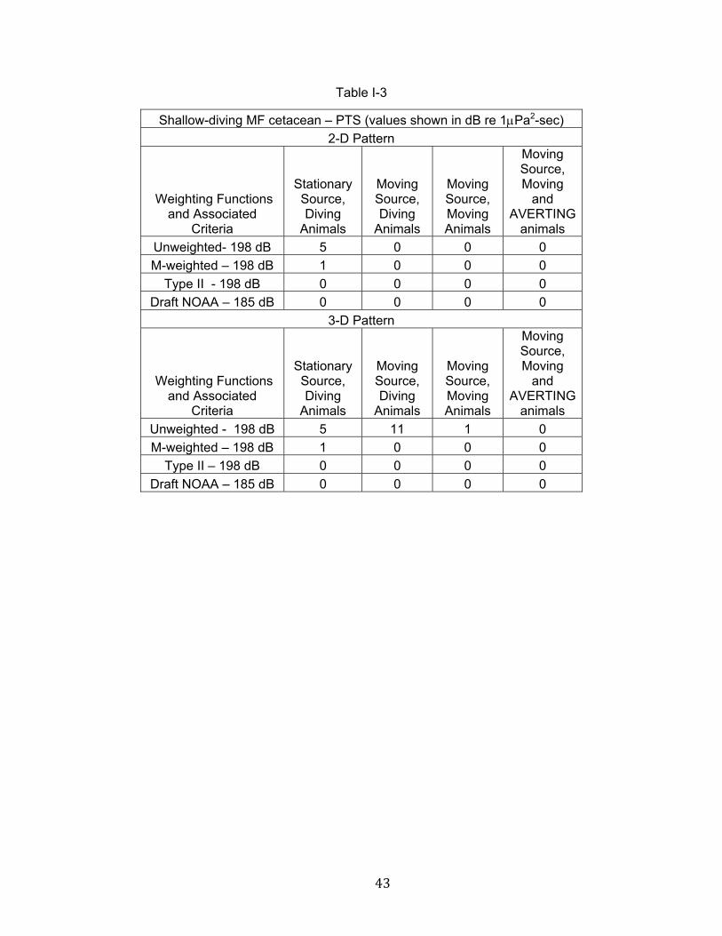
Consideration of Combination of Auditory Weighting Function and Criteria

Theauditoryweighting/criteriaassessmentsaremorecomplexinexplanationduetosubtleeffectsoftheweightingfunctionshapesforM,TypeIIandNOAA(2016)inrelationtothechangesinPTScriteriathatareassociatedwitheachfunction.Theresultof

28

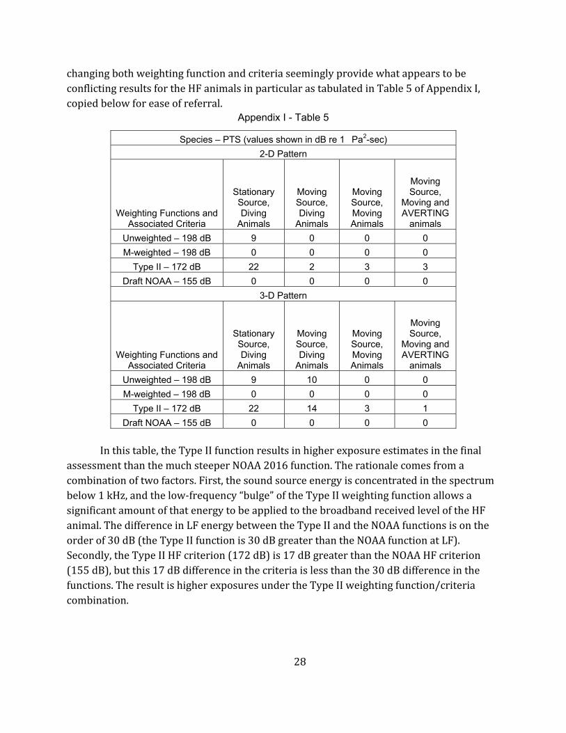
changingbothweightingfunctionandcriteriaseeminglyprovidewhatappearstobeconflictingresultsfortheHFanimalsinparticularastabulatedinTable5ofAppendixI,copiedbelowforeaseofreferral.

Appendix I - Table 5

Species – PTS (values shown in dB re 1�Pa2-sec)

2-D Pattern

Weighting Functions and Associated Criteria

Stationary Source, Diving

Animals

Moving Source, Diving

Animals

Moving Source, Moving Animals

Moving Source,

Moving and AVERTING

animals

Unweighted – 198 dB 9 0 0 0

M-weighted – 198 dB 0 0 0 0

Type II – 172 dB 22 2 3 3

Draft NOAA – 155 dB 0 0 0 0

3-D Pattern

Weighting Functions and Associated Criteria


Animals


Animals


Moving Source,

Moving and AVERTING

animals



Type II – 172 dB 22 14 3 1


Inthistable,theTypeIIfunctionresultsinhigherexposureestimatesinthefinal

assessmentthanthemuchsteeperNOAA2016function.Therationalecomesfromacombinationoftwofactors.First,thesoundsourceenergyisconcentratedinthespectrumbelow1kHz,andthelow‐frequency“bulge”oftheTypeIIweightingfunctionallowsasignificantamountofthatenergytobeappliedtothebroadbandreceivedleveloftheHFanimal.ThedifferenceinLFenergybetweentheTypeIIandtheNOAAfunctionsisontheorderof30dB(theTypeIIfunctionis30dBgreaterthantheNOAAfunctionatLF).Secondly,theTypeIIHFcriterion(172dB)is17dBgreaterthantheNOAAHFcriterion(155dB),butthis17dBdifferenceinthecriteriaislessthanthe30dBdifferenceinthefunctions.TheresultishigherexposuresundertheTypeIIweightingfunction/criteriacombination.

29

Comparison of Long‐term Modeling with Current 24 hour‐reset based regulatory

framework

NOAA’sacousticguidance(NOAA,2016)incorporatestheconceptof“24‐hourreset”inanimalexposureestimates.The“24‐hrreset”meansthattheintegrationtimeforCSELandtheevaluationperiodforbehavioral(maximumSPL)metricsaresetto24hours.Thesemodeloutputvaluesarethencomparedwithregulatorythresholdsandthenumberof‘takes’isdeterminedfora24‐hourperiod.Typically,thesedailynumbersaresimplymultipliedbythenumberofdaysoverwhichtheactivityisanticipatedtooccurtoproducetotaltakeestimates.Thisrequirementhasmeaningfulpracticalimplicationsonmodelingconductedtopredicttheimpactofahumanactivity.

Firstly,thisapproachdoesnotdifferentiatebetweenthenumberof“acousticexposures”andthenumberof“exposedindividuals”.An“acousticexposure”isdefinedhereaswhenanindividualanimalisexposedtoasoundlevelthatexceedsaregulatorythreshold(e.g.,160dBrmsforairguns).An“exposedindividual”isananimalthatexperiencesoneormoreacousticexposuresduringthedurationofanactivity.Givenanimalandsourcemovement,individualanimalscouldexperiencemultipleacousticexposureswithinone24‐hrperiodorovermanydaysofanactivity.

Thisissueiscompoundedwhenanestimateoftheactivity’simpactonapopulationiscomputed.Anactivity’spredictedtakenumbersareoftencomparedtopopulationsizeestimates.Withasufficientlylongactivity,therecanbemore‘24hour’takesthanthereareindividualsinthepopulation.

Apotentialsolutiontothisquandaryisillustratedthroughlong‐termanimatmodeling.Bymodelingtheentiredurationofanactivity,thenumberofexposuresthateachindividualexperiences,aswellasthenumberofexposedanimalsandthetraditionalmetricofthetotalnumberofexposurescanbecalculated.Thusinthisapproach,thenumberofexposedanimalscannotexceedthenumberofanimalsinthepopulation,andthepotentialimpactonindividualanimalsiselucidatedthroughdirectmodelingresults.

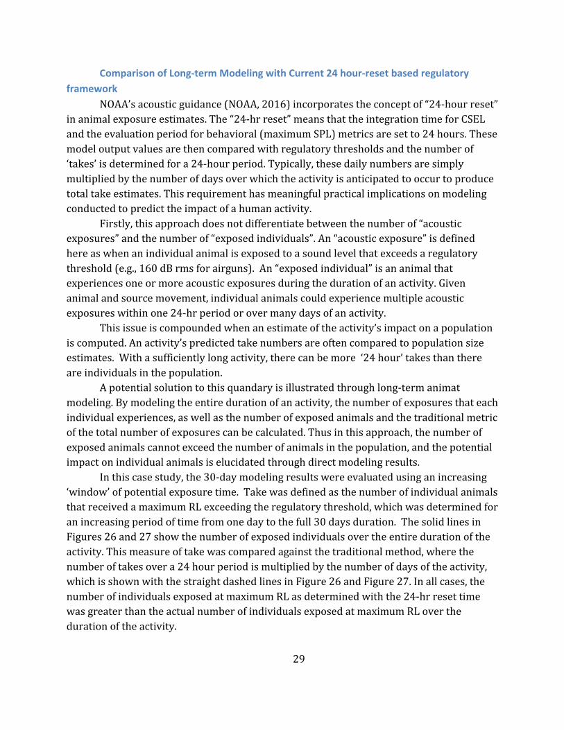
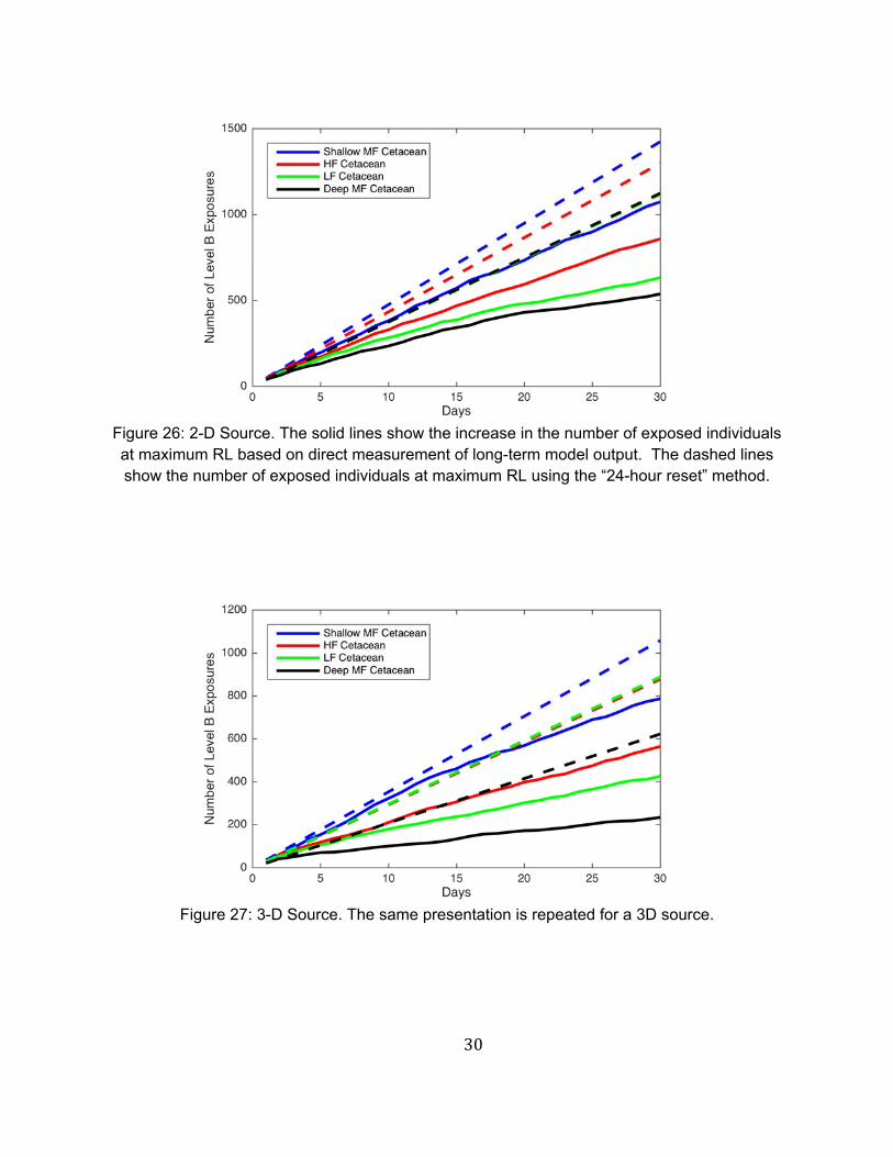
Inthiscasestudy,the30‐daymodelingresultswereevaluatedusinganincreasing‘window’ofpotentialexposuretime.TakewasdefinedasthenumberofindividualanimalsthatreceivedamaximumRLexceedingtheregulatorythreshold,whichwasdeterminedforanincreasingperiodoftimefromonedaytothefull30daysduration.ThesolidlinesinFigures26and27showthenumberofexposedindividualsovertheentiredurationoftheactivity.Thismeasureoftakewascomparedagainstthetraditionalmethod,wherethenumberoftakesovera24hourperiodismultipliedbythenumberofdaysoftheactivity,whichisshownwiththestraightdashedlinesinFigure26andFigure27.Inallcases,thenumberofindividualsexposedatmaximumRLasdeterminedwiththe24‐hrresettimewasgreaterthantheactualnumberofindividualsexposedatmaximumRLoverthedurationoftheactivity.

30

Figure 26: 2-D Source. The solid lines show the increase in the number of exposed individuals at maximum RL based on direct measurement of long-term model output. The dashed lines show the number of exposed individuals at maximum RL using the “24-hour reset” method.

Figure 27: 3-D Source. The same presentation is repeated for a 3D source.

31

Anotherwaytoconsiderthiseffectisahypotheticalpopulationof100individualsforwhich10individualsexperiencemaximumRLsthatexceedtheregulatorythresholdovera24‐hrperiod(i.e.,the‘24hour’takepredictionis10).Overa30‐dayactivity,thetotalpredictedtakewouldbe300(30daysx10animals/day),or3xthepopulationsize.Onecouldassumethattheanimalsinthispopulationhadextremelyhighresidencyorsitefidelity.Insuchacase,itcouldbethatfor30days,thesame10animalsareexposedrepeatedly.Thusthenumberofexposedanimalswasactuallyonly10,while300exposureswerepredicted.

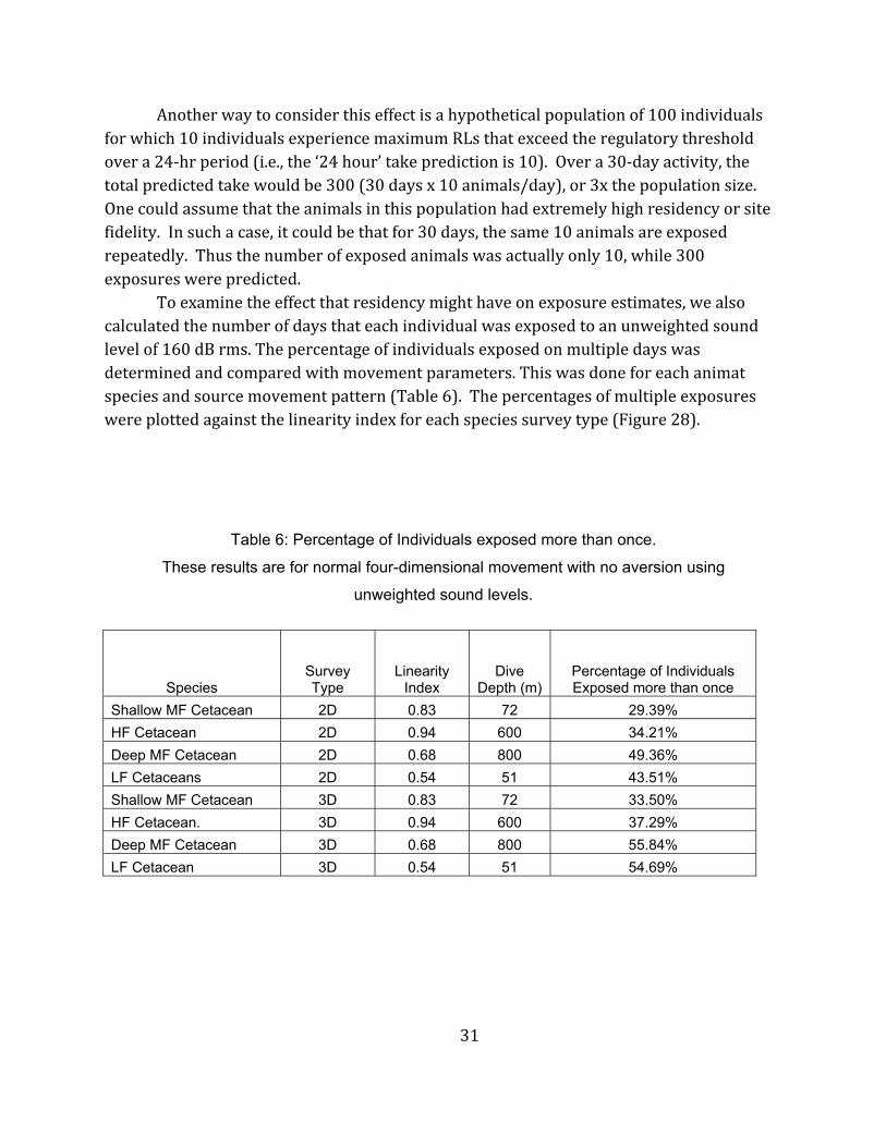
Toexaminetheeffectthatresidencymighthaveonexposureestimates,wealsocalculatedthenumberofdaysthateachindividualwasexposedtoanunweightedsoundlevelof160dBrms.Thepercentageofindividualsexposedonmultipledayswasdeterminedandcomparedwithmovementparameters.Thiswasdoneforeachanimatspeciesandsourcemovementpattern(Table6).Thepercentagesofmultipleexposureswereplottedagainstthelinearityindexforeachspeciessurveytype(Figure28).

Table 6: Percentage of Individuals exposed more than once.

These results are for normal four-dimensional movement with no aversion using

unweighted sound levels.

Species Survey Type

Linearity Index

Dive Depth (m)

Percentage of Individuals Exposed more than once

Shallow MF Cetacean 2D 0.83 72 29.39%

HF Cetacean 2D 0.94 600 34.21%

Deep MF Cetacean 2D 0.68 800 49.36%

LF Cetaceans 2D 0.54 51 43.51%

Shallow MF Cetacean 3D 0.83 72 33.50%

HF Cetacean. 3D 0.94 600 37.29%

Deep MF Cetacean 3D 0.68 800 55.84%

LF Cetacean 3D 0.54 51 54.69%

32

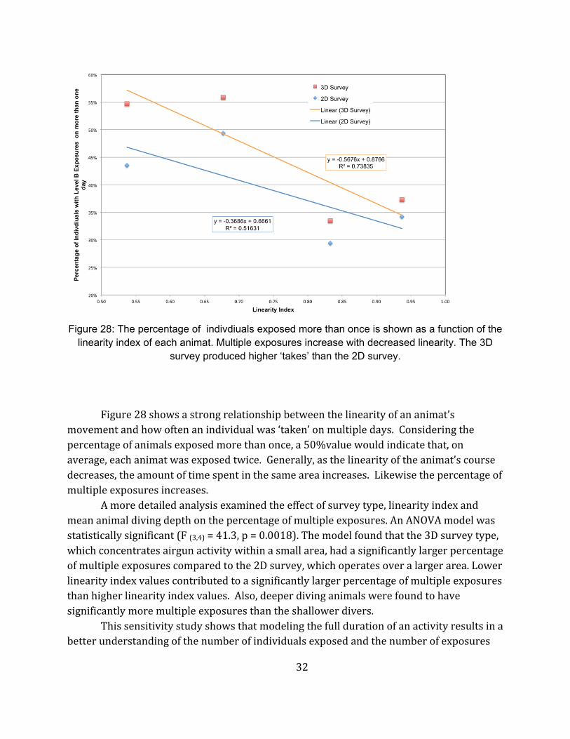
Figure 28: The percentage of indivdiuals exposed more than once is shown as a function of the

linearity index of each animat. Multiple exposures increase with decreased linearity. The 3D survey produced higher ‘takes’ than the 2D survey.

Figure28showsastrongrelationshipbetweenthelinearityofananimat’smovementandhowoftenanindividualwas‘taken’onmultipledays.Consideringthepercentageofanimalsexposedmorethanonce,a50%valuewouldindicatethat,onaverage,eachanimatwasexposedtwice.Generally,asthelinearityoftheanimat’scoursedecreases,theamountoftimespentinthesameareaincreases.Likewisethepercentageofmultipleexposuresincreases.

Amoredetailedanalysisexaminedtheeffectofsurveytype,linearityindexandmeananimaldivingdepthonthepercentageofmultipleexposures.AnANOVAmodelwasstatisticallysignificant(F(3,4)=41.3,p=0.0018).Themodelfoundthatthe3Dsurveytype,whichconcentratesairgunactivitywithinasmallarea,hadasignificantlylargerpercentageofmultipleexposurescomparedtothe2Dsurvey,whichoperatesoveralargerarea.Lowerlinearityindexvaluescontributedtoasignificantlylargerpercentageofmultipleexposuresthanhigherlinearityindexvalues.Also,deeperdivinganimalswerefoundtohavesignificantlymoremultipleexposuresthantheshallowerdivers.

Thissensitivitystudyshowsthatmodelingthefulldurationofanactivityresultsinabetterunderstandingofthenumberofindividualsexposedandthenumberofexposures

33

perindividual.Thesearekeyparametersfordeterminingpotentialimpacts,particularlyforprotectedspecies.Thereforebothmetricscouldbeevaluatedandsuchanapproachwouldprovideinsightintotraditionalpredictionsoftakenumberslargerthanpopulationsizes.

Thevalidityofthelong‐durationmodelingresultsarestronglyinfluencedbytheaccuracyofthebehavioralparametersusedtocreatethesimulations.Reliabledataontheresidencypatternsanddivingbehaviorsofspeciesandpopulationsbeingmodelediscriticaltovalidmodeloutputs.

Considering the effect of group size on number of predicted exposures

Thebasicmodelingapproachconsistsofcreatingan‘overpopulated’simulation,wherethemodeldensityistypicallymuchgreaterthanthatofthereal‐worldsituationandeachanimatrepresentsanindividualanimal.Oncethesimulationhasbeenrun,theoutputsareexaminedtodeterminethenumberofexposuresthatexceedregulatorythresholds.Whenanimatsareconsideredasindividuals,thescalingrelationshipisquitesimple,asexpressedinthefollowingequation.

∗

Typically,thenumberofmodeledexposuresisapointestimatebasedonthemodelingresults.However,anestimateofuncertaintyintheexposureestimatescanbecalculatedusingresampling,inwhichcasethemodeledexposuresvaluecouldbeameanofresampledestimateswithanassociatedmeasureofvariation(e.g.,S.D.orC.V.).

Tomovethemodelingscenariotowardsamorerealisticreflectionofanimaldistribution,however,itisimportanttoconsiderthatmostanimalsnaturallyoccuringroupsofvariablesize.Themeanvalueofanexposureestimatewillnotchangebecausethedensityofanimalgroupsistheindividualanimaldensityvalue(animals/area)dividedbythemeangroupsize.Thefactorthatwillchangeisthemeasureofvariationaroundthatmean,whichreflectsthevariabilityinthedistributionofgroupsizeinwildpopulations.

Themoststraightforwardapproachtoincorporatinggroupsizeintotheeffectsanalysisistousearesamplingprocedure.Inthisstudy,asetofdistributionsofgroupsizeswascreatedbasedonobservedgroupsizeestimates(Maze‐FoleyandMullin,2006),asshowninTable7.Groupsizeminimumandmaximumvalueswerecreatedforeachspeciesusingalognormalfunction,roundedtointegersandtruncatedtothelargestreportedgroupsize.

Bothindividualsandgroupshaveacommonsourceofvariabilityinhowmanyanimatsinaselectedsamplewillhaveareceivedlevelthatexceedsaregulatorythreshold.GroupSizeintroducesanadditionalsourceofvariation(i.e.,thenumberofanimalsrepresentedbyasingleanimat)notfoundintheindividualanalysis.Therefore,withtwosourcesofvariation,theaprioiriexpectationisthatthevariancearoundthegroup‐basedmeanestimateshouldbegreaterthanthatforindividuals.

34

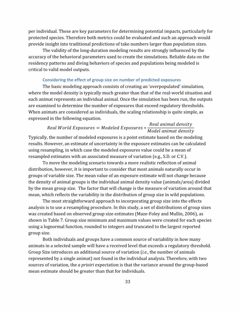
Table 7: Group Size Data for Gulf of Mexico

Animat Type Mean

Group Size SE Min Max N

LF Cetacean 2.0 0.33 1 5 14

Deep MF Cetacean 2.6 0.16 1 11 164

HF Cetacean 2.0 0.12 1 8 133

Shallow MF Cetacean 20.6 2.49 1 220 151

Theresamplingprocedureselected100samplesfromtheacousticexposuredata

andthegroupsizedistribution.Thenumberofsamplesthatexceededaregulatorythreshold(e.g.,160dBRMS)alongwiththeircorrespondinggroupsizewasdetermined.Thesumofthegroupsizesampleswasreturnedasthenumberofindividualsexposedtothatthresholdlevel.Thisprocesswasrepeated10,000timestoproducearesampleddistributionofthenumberofexposedindividuals.Themeanandstandarddeviationoftheseresampleddistributionswerecalculated.Thustheresamplingapproachprovidesanadditionalmethodtoestimatingconfidencelimitsaroundtheexposureestimate.

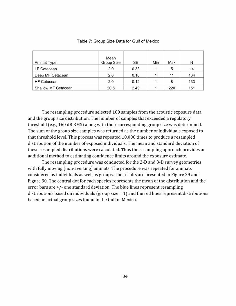
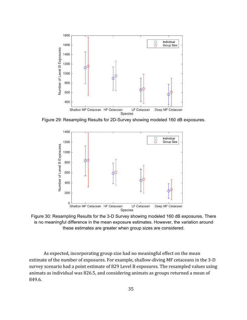
Theresamplingprocedurewasconductedforthe2‐Dand3‐Dsurveygeometrieswithfullymoving(non‐averting)animats.Theprocedurewasrepeatedforanimatsconsideredasindividualsaswellasgroups.TheresultsarepresentedinFigure29andFigure30.Thecentraldotforeachspeciesrepresentsthemeanofthedistributionandtheerrorbarsare+/‐onestandarddeviation.Thebluelinesrepresentresamplingdistributionsbasedonindividuals(groupsize=1)andtheredlinesrepresentdistributionsbasedonactualgroupsizesfoundintheGulfofMexico.

35

Figure 29: Resampling Results for 2D-Survey showing modeled 160 dB exposures.

Figure 30: Resampling Results for the 3-D Survey showing modeled 160 dB exposures. There

is no meaningful difference in the mean exposure estimates. However, the variation around these estimates are greater when group sizes are considered.

Asexpected,incorporatinggroupsizehadnomeaningfuleffectonthemeanestimateofthenumberofexposures.Forexample,shallow‐divingMFcetaceansinthe3‐Dsurveyscenariohadapointestimateof829LevelBexposures.Theresampledvaluesusinganimatsasindividualwas826.5,andconsideringanimatsasgroupsreturnedameanof849.6.

36

Inallcasesthestandarddeviationsweregreaterwhenanimatswereconsideredasgroupsratherthanindividuals.Furthermore,thesizeofthestandarddeviationincreasedasafunctionofgroupsize.Thusitcanbeconcludedthatincorporatinggroupsizeestimatedatawill(realistically)increasetheuncertaintyaroundthemeannumberofpredictedexposureswithoutmeaningfullychangingitsvalue.

Considering the Effect of Movement of Sources and Animals

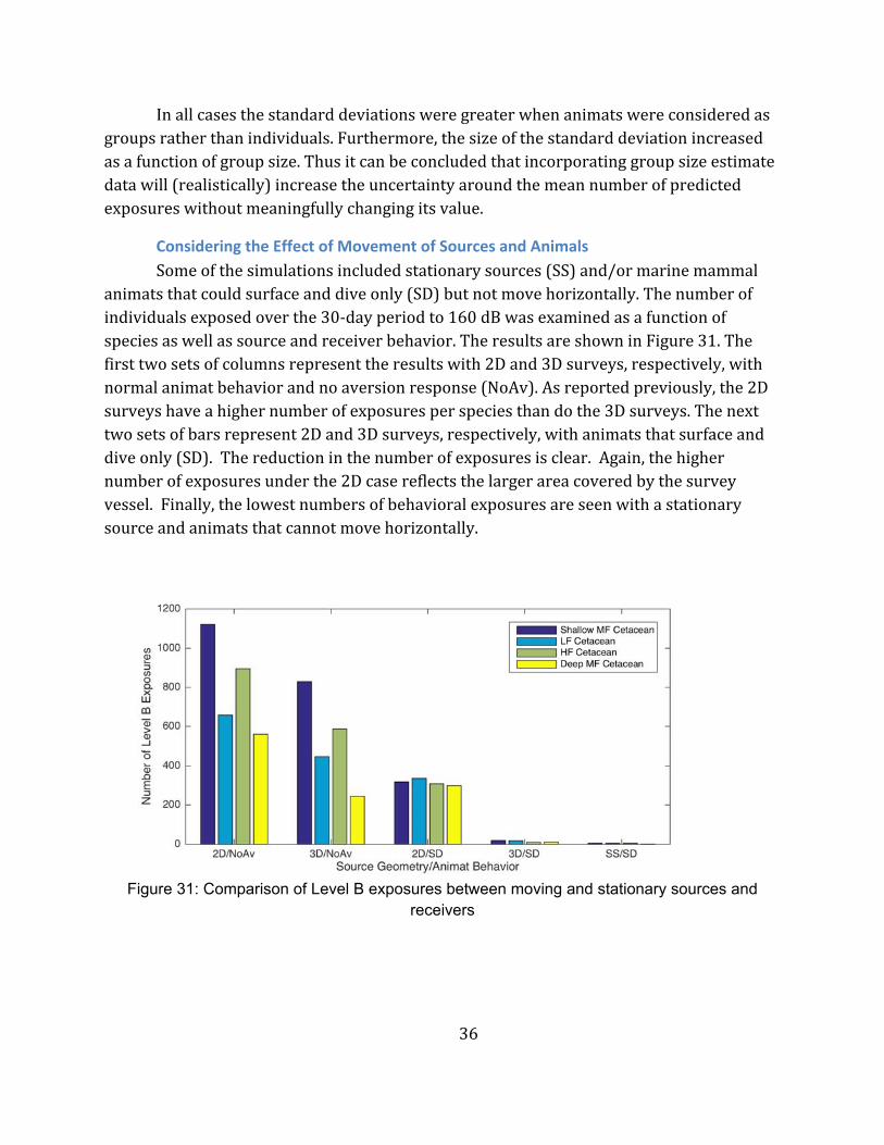
Someofthesimulationsincludedstationarysources(SS)and/ormarinemammalanimatsthatcouldsurfaceanddiveonly(SD)butnotmovehorizontally.Thenumberofindividualsexposedoverthe30‐dayperiodto160dBwasexaminedasafunctionofspeciesaswellassourceandreceiverbehavior.TheresultsareshowninFigure31.Thefirsttwosetsofcolumnsrepresenttheresultswith2Dand3Dsurveys,respectively,withnormalanimatbehaviorandnoaversionresponse(NoAv).Asreportedpreviously,the2Dsurveyshaveahighernumberofexposuresperspeciesthandothe3Dsurveys.Thenexttwosetsofbarsrepresent2Dand3Dsurveys,respectively,withanimatsthatsurfaceanddiveonly(SD).Thereductioninthenumberofexposuresisclear.Again,thehighernumberofexposuresunderthe2Dcasereflectsthelargerareacoveredbythesurveyvessel.Finally,thelowestnumbersofbehavioralexposuresareseenwithastationarysourceandanimatsthatcannotmovehorizontally.

Figure 31: Comparison of Level B exposures between moving and stationary sources and

receivers

37

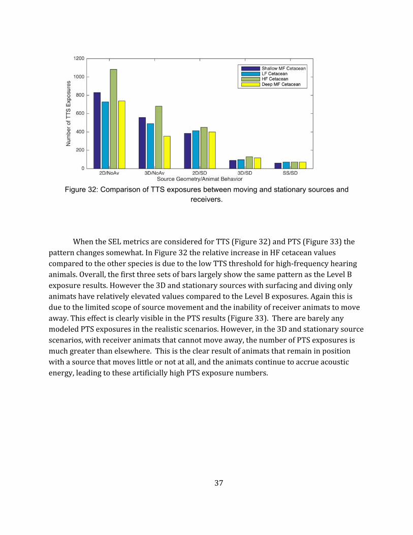
Figure 32: Comparison of TTS exposures between moving and stationary sources and

receivers.

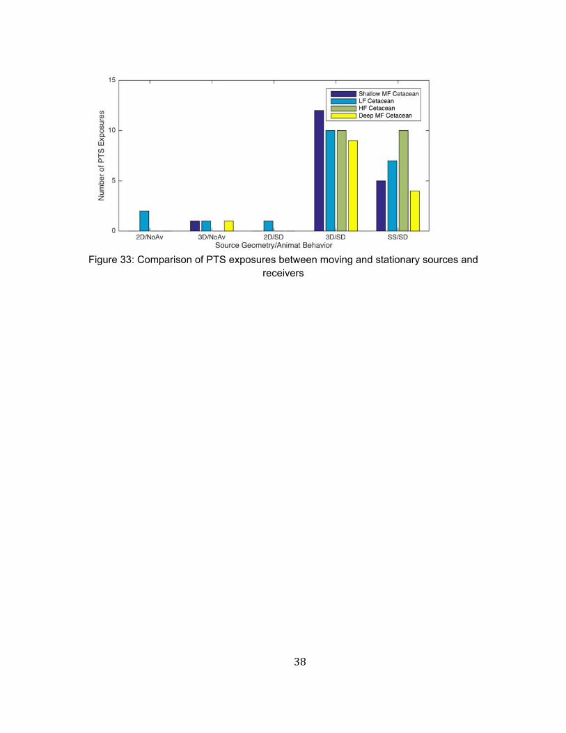
WhentheSELmetricsareconsideredforTTS(Figure32)andPTS(Figure33)thepatternchangessomewhat.InFigure32therelativeincreaseinHFcetaceanvaluescomparedtotheotherspeciesisduetothelowTTSthresholdforhigh‐frequencyhearinganimals.Overall,thefirstthreesetsofbarslargelyshowthesamepatternastheLevelBexposureresults.Howeverthe3DandstationarysourceswithsurfacinganddivingonlyanimatshaverelativelyelevatedvaluescomparedtotheLevelBexposures.Againthisisduetothelimitedscopeofsourcemovementandtheinabilityofreceiveranimatstomoveaway.ThiseffectisclearlyvisibleinthePTSresults(Figure33).TherearebarelyanymodeledPTSexposuresintherealisticscenarios.However,inthe3Dandstationarysourcescenarios,withreceiveranimatsthatcannotmoveaway,thenumberofPTSexposuresismuchgreaterthanelsewhere.Thisistheclearresultofanimatsthatremaininpositionwithasourcethatmoveslittleornotatall,andtheanimatscontinuetoaccrueacousticenergy,leadingtotheseartificiallyhighPTSexposurenumbers.

38

Figure 33: Comparison of PTS exposures between moving and stationary sources and

receivers

39

Literature Cited

Baker,C.S.,andL.M.Herman.(1989).Thebehavioralresponsesofsummeringhumpbackwhalestovesseltraffic:Experimentalandopportunisticobservations.Honolulu

Burdic,W.S.(1984).UnderwaterAcousticSystemAnalysis.EnglewoodCliffs,NJ:Prentice‐Hall,Inc.

Collins,M.D.(1993).Asplit‐stepPadésolutionfortheparabolicequationmethod.TheJournaloftheAcousticalSocietyofAmerica,93(4),1736‐1742.

Cordue,P.(2006).SummaryReport:ReviewoftheAcousticIntegrationModel25‐27September2006,WashingtonDC

Ellison,W.T.,R.Racca,C.W.Clark,B.Streever,A.S.Frankel,E.Fleishman,R.Angliss,J.Berger,D.Ketten,M.Guerra,M.Leu,M.McKenna,T.Sformo,B.Southall,R.Suydam,andL.Thomas.(2016).ModelingtheaggregatedexposureandresponsesofbowheadwhalesBalaenamysticetustomultiplesourcesofanthropogenicunderwatersound.EndangeredSpeciesResearch,30,95‐108.doi:10.3354/esr00727

Finneran,J.J.,andA.K.Jenkins.(2012).CriteriaandThresholdsforU.S.NavyAcousticandExplosiveEffectsAnalysis

Frankel,A.S.,W.T.Ellison,andJ.Buchanan.(2002).ApplicationoftheAcousticIntegrationModel(AIM)topredictandminimizeenvironmentalimpacts.IEEEOceans2002,1438‐1443.

Hatton,L.(2008).Gundalf–anairgunarraymodellingpackage.Retrievedfromhttp://www.gundalf.com

Maze‐Foley,K.,andK.D.Mullin.(2006).CetaceansoftheoceanicnorthernGulfofMexico:Distributions,groupsizesandinterspecificassociations.JournalofCetaceanResearchandManagement,8(2),203‐213.

NationalOceanicandAtmosphericAdministration(NOAA).(2016).ProposedChangesTo:NationalOceanicAndAtmosphericAdministrationDraftGuidanceForAssessingTheEffectsOfAnthropogenicSoundOnMarineMammalHearingUnderwaterAcousticThresholdLevelsForOnsetOfPermanentAndTemporaryThresholdShiftsSilverSpring

NavalOceanographicOffice.(2003).Databasedescriptionforthegeneralizeddigitalenvironmentalmodel(GDEMV)(U),version3.0

Southall,B.L.,A.E.Bowles,W.T.Ellison,J.J.Finneran,R.L.Gentry,C.R.Greene,Jr.,D.Kastak,D.R.Ketten,J.H.Miller,P.E.Nachtigall,W.J.Richardson,J.A.Thomas,andP.

40

L.Tyack.(2007).Marinemammalnoiseexposurecriteria:InitialscientificrecommendationsAquaticMammals,33(4),411‐521.

Weinberg,H.(2004).CASSUser'sGuide.AntonInternationalCorporation

Zeddies,D.G.,M.Zykov,H.Yurk,T.Deveau,L.Bailey,I.Gaboury,R.Racca,D.Hannay,andS.Carr.(2015).AcousticPropagationandMarineMammalExposureModelingofGeologicalandGeophysicalSourcesintheGulfofMexico:2016–2025AnnualAcousticExposureEstimatesforMarineMammals.JASCODocument00976,Version2.0.TechnicalreportbyJASCOAppliedSciencesforBureauofOceanEnergyManagement(BOEM)

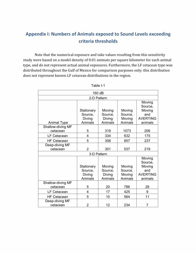
Appendix I: Numbers of Animals exposed to Sound Levels exceeding

criteria thresholds

Notethatthenumericalexposureandtakevaluesresultingfromthissensitivity

studywerebasedonamodeldensityof0.01animatspersquarekilometerforeachanimaltype,anddonotrepresentactualanimalexposures.Furthermore,theLFcetaceantypewasdistributedthroughouttheGulfofMexicoforcomparisonpurposesonly;thisdistributiondoesnotrepresentknownLFcetaceandistributionsintheregion.

Table I-1

160 dB

2-D Pattern

Animal Type


Animals


Animals


Moving Source, Moving

and AVERTING

animals Shallow-diving MF

cetacean 5 319 1073 206

LF Cetacean 4 334 632 175

HF Cetacean 5 308 857 237 Deep-diving MF

cetacean 2 301 537 219

3-D Pattern


Animals


Animals



and AVERTING


cetacean 5 20 786 28



cetacean 2 12 234 7

42

Table I-2

180 dB

2-D Pattern

Animal Type


Animals


Animals



and AVERTING


cetacean 0 25 26 0



cetacean 0 25 43 15

3-D Pattern


Animals


Animals



and AVERTING


cetacean 0 13 17 0



cetacean 0 8 26 0

43

Table I-3

Shallow-diving MF cetacean – PTS (values shown in dB re 1Pa2-sec)

2-D Pattern

Weighting Functions and Associated

Criteria


Animals


Animals



and AVERTING

animals

Unweighted- 198 dB 5 0 0 0


Type II - 198 dB 0 0 0 0


3-D Pattern


Criteria


Animals


Animals



and AVERTING

animals

Unweighted - 198 dB 5 11 1 0


Type II – 198 dB 0 0 0 0


44

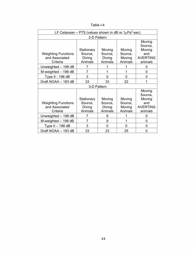
Table I-4

LF Cetacean – PTS (values shown in dB re 1Pa2-sec)

2-D Pattern


Criteria


Animals


Animals



and AVERTING

animals



Type II - 198 dB 3 0 0 0

Draft NOAA – 183 dB 33 33 22 1

3-D Pattern


Criteria


Animals


Animals



and AVERTING

animals



Type II – 198 dB 3 0 0 0

Draft NOAA – 183 dB 33 23 25 0

45

Table I-5

HF Cetacean Species – PTS (values shown in dB re 1Pa2-sec)

2-D Pattern


Criteria


Animals


Animals



and AVERTING

animals



Type II – 172 dB 22 2 3 3


3-D Pattern


Criteria


Animals


Animals



and AVERTING

animals



Type II – 172 dB 22 14 3 1


46

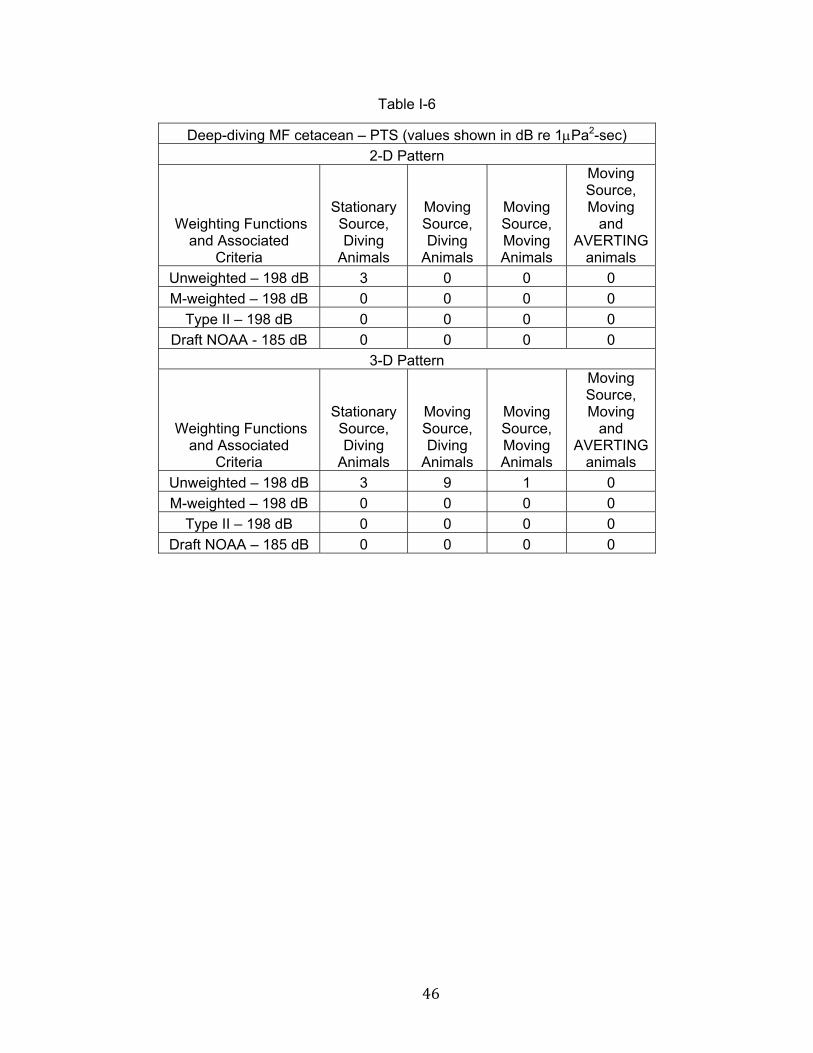
Table I-6

Deep-diving MF cetacean – PTS (values shown in dB re 1Pa2-sec)

2-D Pattern


Criteria


Animals


Animals



and AVERTING

animals



Type II – 198 dB 0 0 0 0

Draft NOAA - 185 dB 0 0 0 0

3-D Pattern


Criteria


Animals


Animals



and AVERTING

animals



Type II – 198 dB 0 0 0 0


Documents

JIP Aversion Modeling Final Report Adam S. Frankel, …gisserver.intertek.com/JIP/DMS/ProjectReports/Cat2/Frankel2016... · JIP Aversion Modeling Final Report Adam S. Frankel, Ph.D