Embed Size (px)
Citation preview
jitSim: A Simulator for Predicting Scalability of
Parallel Applications in Presence of OS Jitter
Pradipta De and Vijay Mann
IBM Research - India, New Delhi
Abstract. Traditionally, Operating system jitter has been a source ofperformance degradation for parallel applications running on large num-ber of processors. While some large scale HPC systems such as BlueGene/L and Cray XT4, mitigate jitter by making use of a specializedlight-weight operating system on compute nodes, other clusters haveattempted using HPC-ready commodity operating systems such as Zep-toOS (based on Linux). However, as large systems continue to be de-signed to work with commodity OSes, OS jitter still remains an activearea of research within the HPC community. While, it is true that someof the specialized commodity OSes like ZeptoOS have relatively low OSjitter levels, there is still a need to have a quick and easy set of toolsthat can predict the impact of OS jitter at a given configuration andprocessor number. Such tools are also required to validate and compareany new techniques or OS enhancements that mitigate jitter. Emulatingjitter on a large ”jitter-free” platform using either synthetic jitter or realtraces from commodity OSes has been proposed as one useful mechanismto study scalability behavior under the presence of jitter. However, thisrequires access to large scale jitter free systems, which are few in numberand not so easily accessible. As new systems are built, that should scaleup to a million tasks and more, the emulation approach is still limitedby the largest jitter free system available. In this paper we present jitSim- a simulation framework for predicting scalability of parallel computeintensive applications in presence of OS jitter using trace driven simula-tion. The jitter simulation framework can be used to quickly simulate theeffects of jitter that is characteristic of a given OS using a given trace.Furthermore, this system can be used to predict scalability up to anyarbitrarily large number of task counts. Our methodology comprises ofcollection of real jitter traces, measurement of network latency, messagepassing stack latency, and shared memory latency. The simulation frame-work takes the above as inputs and then simulates multiple parallel tasksstarting at randomly chosen points in the jitter trace and executing acompute phase. We validate the simulation results by comparing it withreal data and demonstrate the efficacy of the simulation framework byevaluating various jitter mitigation techniques through simulation.
1 Introduction
Operating system jitter (or OS jitter) refers to the interference experienced byan application due to scheduling of background daemon processes and handling
P.D’Ambra,M.Guarracino, andD.Talia (Eds.):Euro-Par 2010, Part I, LNCS6271, pp. 117–130, 2010.c© Springer-Verlag Berlin Heidelberg 2010
118 P. De and V. Mann
of asynchronous events such as interrupts. It has been shown that parallel ap-plications on large clusters suffer considerable degradation in performance dueto OS jitter [1,2].
Techniques to mitigate jitter fall broadly under four categories: use of micro-kernels, OS and hardware level tuning techniques [3], synchronization of jitter[4,5] and enhancements to popular commodity OSes [6]. Several large scale HPCsystems, like the Blue Gene/L [7] and Cray XT4 [8], make use of a customizedlight-weight microkernel at the compute nodes to mitigate OS jitter. These cus-tomized kernels typically do not support general purpose multitasking and maynot even support interrupts. However, these systems require applications to bemodified or ported to their respective platforms. Other systems like the ASCIPurple and the JS21 system at the Barcelona Supercomputing Center [9], whichmake use of commodity OSes (AIX and RedHat Enterprise Linux respectively),still suffer from OS jitter [10]. These systems rely mainly on OS and hardwarelevel tuning and/or synchronization of jitter across nodes. Synchronization ofjitter across all nodes can yield moderate (close to 50% [4]) to very high (closeto 300% [5]) performance improvements. Simultaneous multi threaded (SMT)and hyperthreaded processors can also help in mitigating jitter, even thoughthey may have other performance implications. The ZeptoOS project [6] fromArgonne National Laboratory has been working on making Linux HPC-readyon compute nodes as well as I/O nodes.
While, it is true that some of the specialized commodity OSes like ZeptoOShave relatively low OS jitter levels, OS jitter still remains an active area of re-search within the HPC community as researchers continue to explore applicationsensitivity to jitter levels in their clusters [11]. As large systems continue to bedesigned to work with commodity OSes [12,13,6], there is a need to have a quickand easy set of tools that can predict the impact of OS jitter at a given config-uration and number of processors. Such tools are also required to validate andcompare any new techniques or OS enhancements that mitigate jitter. As theeffectiveness of any technique to mitigate jitter can only be evaluated in a largecluster with thousands of nodes, one of the biggest hindrances in the develop-ment and evaluation of new techniques for handling jitter is that there are a fewlarge clusters running commodity OSes worldwide, which are often unavailablefor experimental and validation purposes.
Emulating jitter on a large “jitter-free” platform using either synthetic jitteror real traces from commodity OSes has been proposed as useful mechanism tostudy scalability behavior under the presence of jitter [11,14,15]. Beckman etal. [15] used a single node benchmark to measure jitter and injected syntheticjitter of varying length and periodicity on a jitter-less platform such as BlueGene/L to study its impact on scalability of various collective operations. Theyused purely synthetic jitter rather than collecting traces from real Linux systems.In an earlier work, we improved upon their emulation technique to ensure preciseemulation of jitter [14]. Ferreira et al. [11], in their Supercomputing 2008 (SC2008) paper, described the effect of different kinds of kernel-generated noise onapplication performance at scale.
jitSim: A Simulator for Predicting Scalability of Parallel Applications 119
All the above approaches to predict system performance require an accuratemethodology for precisely emulating jitter. Emulation of jitter on large ”jitterfree” platforms requires access to large scale jitter free systems. As new systemsare built that should scale up to a million tasks and more, the emulation approachis still limited by the largest jitter free system available. In this paper, we presentthe design and implementation of jitSim - a simulation framework for predictingscalability of parallel compute intensive applications in presence of OS jitterusing trace driven simulation. The jitter simulation framework can be used toquickly simulate the effects of jitter that is characteristic of a given OS usinga given trace. Furthermore, this system can be used to predict scalability upto any arbitrarily large number of task counts. The methodology is based oncollection of real jitter traces, measurement of network, message passing stack,and shared memory latencies and simulation of multiple parallel tasks startingat randomly chosen points in the trace that use the cycles between jitter eventsin the trace as the available compute cycles to reach a given number of computephase cycles. We validate the simulation results by comparing it with real dataand demonstrate the efficacy of the simulation framework by evaluating variousjitter mitigation techniques through simulation.
The rest of this paper is organized as follows. Section 2 describes the chal-lenges involved in simulating OS jitter and gives an overview of our approach.Section 3 gives the details of the jitter simulator framework. Section 4 presentsour results. We present an overview of related research in section 5 and finallyconclude in section 6.
2 Methodology
In this section we first describe the challenges involved in simulating the effectsof OS jitter. We then give an overview of our methodology.
2.1 Challenges
Any methodology for predicting scalability of parallel applications in presenceof OS jitter using trace driven simulation faces the following challenges:
– Collection of a trace that is representative of OS Jitter on a real system– Simulation of the synchronization step in a parallel application
• Requires knowledge of network topology, system architecture, number ofcores on a single chip, number of chips in a node
• Requires measurement of one hop network latency, latency in the mes-sage passing stack, shared memory access latency
• Requires knowledge of the synchronization algorithm in the messagepassing layer (e.g. a binary tree, a k-ary tree, an octet tree, etc)
– Different types of applications are likely to be affected differently by OSjitter and will therefore, have a different scaling behavior.
120 P. De and V. Mann
In this paper, we present a methodology that is aware of the above challenges andovercomes them. We collect jitter traces using a microbenchmark that ensuresthat it does not introduce any additional jitter of its own. We collect informationabout one hop network latency, latency in the message passing stack and sharedmemory access latency through various micorexperiments. This work assumesthe parallel application to be a compute intensive application. For a real appli-cation to fit into this model, we require that the application be modeled as asequence of compute, communication and jitter phases. The jitter phases willcomprise of various application induced latencies such as memory access latencyor I/O latency.
2.2 Overall Approach
Our overall approach comprises of the following steps:
1. A large jitter trace is collected from a single core, or a set of cores. The jittertrace is collected using a timestamp reader benchmark, which is explainedlater.
2. one hop network latency, MPI stack latency, shared memory access latencyusing SEND/RECV messages of varying sizes between MPI tasks runningon same nodes and those running on the same node (but different cores) aremeasured.
3. Different portions of the trace can be thought of as multiple traces collectedon different nodes - can be used to model jitter experienced by multipletasks.
4. Different MPI tasks start their simulation from an index at any randompoint in the trace (for baseline) or at any random point that represents thestart of a high priority window (for co-scheduler) or at the same randomlychosen point (for perfectly synchronized jitter).
5. Cycles between two jitter events in trace are used as available compute cyclesand the total cycles consumed by each task (which include jitter cycles andcompute cycles) are calculated to complete a compute phase.
6. A synchronization point is simulated across all tasks at the end of a computephase by passing send and receive messages (using the latencies measuredearlier) across the tasks arranged in a tree.
7. A slowdown is calculated by by comparing the total consumed cycles to thecompute cycles.
These steps are described in more detail in the sections below.
3 Implementation Details
In this section we describe in detail the steps involved in our simulationmethodology.
jitSim: A Simulator for Predicting Scalability of Parallel Applications 121
3.1 Collection of a Jitter Trace
We use a single node timestamp register reader benchmark (which we refer to asthe TraceCollector) for collecting a jitter trace. The TraceCollector is run on asingle node that is running the operating system with the specific configurationunder which we want to predict the cluster scalability. The TraceCollector has atight loop that reads the timestamp counter register repeatedly and finds out thetimestamp deltas between successive readings. It then compares each timestampdelta with the minimum timestamp delta (tmin) observed on that platform todecide whether that timestamp delta constitutes a jitter instance or not. Thisis used to create a jitter distribution as well as a jitter trace. Each core runs aunique instance of TraceCollector and a trace is generated for each core. Thejitter trace is a tuple of the form: < jitter duration, cycles to next jitter >.More details about trace collection can be found in [16].
3.2 Measurement of Message Passing Latencies
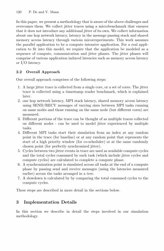
When parallel tasks run on the same physical node in a system, they typicallycommunicate over shared memory whereas when they run on different physicalnodes, they communicate over the network using the high speed interconnect.In order to simulate a tree based synchronization point (for example, a barrier)across tasks, these latencies need to be measured. Three experiments are con-ducted to estimate one hop, network latency, MPI Stack Latency and SharedMemory Latency. In each experiment, two MPI tasks are run either on two coresof the same node (for measuring shared memory access latency or the MPI stacklatency) or on two different physical nodes (for measuring one hop network la-tency) and MPI SEND and RECV messages of varying sizes are passed betweenthese two tasks and finally an average is calculated. These experiments are shownin Figure 1. MPI Stack latency is divided by half to get an estimate of SEND andRECV latencies. MPI tasks are allocated sequentially among the cores followedby nodes.
3.3 Simulating Multiple Parallel Tasks Using a Single Jitter Trace
Different portions of the trace can be thought of as multiple traces collected ondifferent nodes and hence can be used to model jitter experienced by multipletasks.
Fig. 1. Measurement of communication latencies
122 P. De and V. Mann
Choosing the point in the jitter trace from where the different tasks startexecuting is an important decision and it can have interesting ramifications. In acluster that has unsynchronized jitter, different kinds of jitter activities will hiteach node at different points in time. On the other hand, in a cluster that hasemployed a mechanism for synchronizing jitter across all nodes, jitter activitieswill hit each node at the same time. In order to emulate the unsynchronized jitterscenario, simulation starts different tasks at different randomly chosen pointsin the jitter trace. To simulate synchronized jitter, simulation starts differenttasks from the same randomly chosen point in the jitter trace. To simulate co-scheduled jitter [5], where a user level co-scheduler daemon puts the favoredprocess into high priority for a given time window (referred to as high prioritywindow) and then into low priority for a short time window (referred to as lowpriority window), the different parallel tasks start at any random point in thetrace that represents the start of a high priority window. This is explained indetail with the help of an example in section 4.
3.4 Simulating Effects of Jitter on a Parallel Application
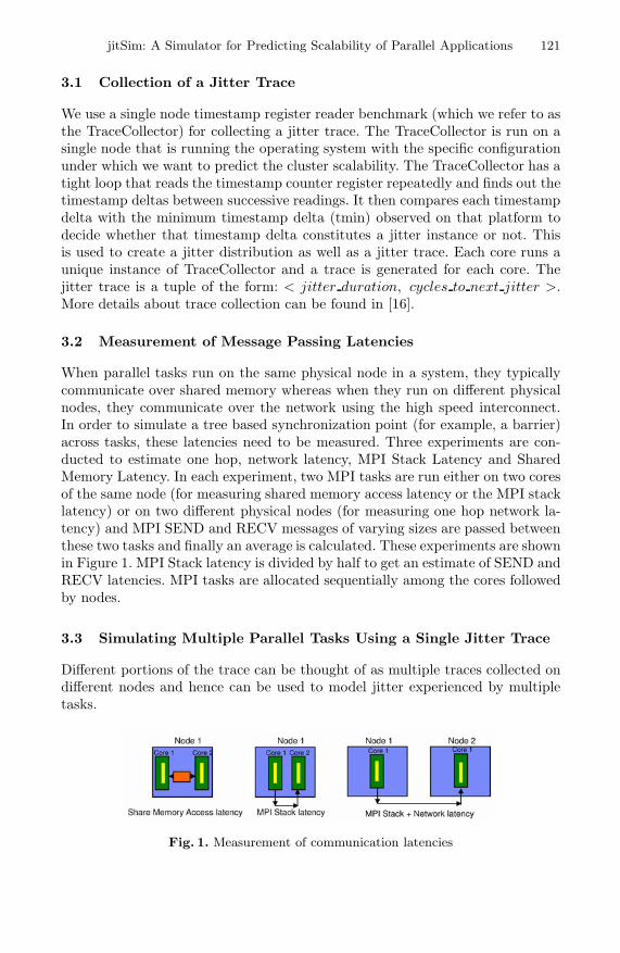
The simulator is a cycle accurate simulator that takes as input a jitter trace,work quanta value in time and frequency of the platform from where the tracehas been collected. It first converts the time work quanta into the target computecycles in each phase by multiplying it by the frequency value. Cycles betweentwo jitter events in trace are used as available compute cycles that can be usedby the parallel task. At each task, it keeps adding the available compute cyclestill a jitter value is reached or the target compute cycles for a compute phase
7010
205
6060
2010
30020
10015
105
2025
305
5010
Cycles_to_next_jitterJitter duration
Simulation of a compute phase -- 2 nodes - no barrier
Compute cycles = 50 + 30 + 20 = 100
Jitter = 5 + 25 = 30
Total cycles to finish a compute phase = 130
Compute cycles = 20 + 60 + 20 = 100
Jitter = 60 + 5 = 65
Total cycles to finish a compute phase = 165
Target Compute Cycles = 100
NODE 2
NODE 1
Randomly chosen portion of trace for Node 1
Randomly chosen portion of trace for Node 2
Fig. 2. Simulation of a compute phase with 2 parallel tasks
jitSim: A Simulator for Predicting Scalability of Parallel Applications 123
95
Node 1 Node 2
Wait cycles at Barrier
7010
205
6060
2010
30020
15
105
2025
305
5010
Cycles_to_next_jitterJitter durationStart of Compute Phase 1
End of Compute
Compute cycles
Jitter cycles
Simulation of a compute phase2 nodes – with wait at the barrier
Randomly chosen portion of trace forNode 1Randomly chosen portion of trace forNode 2Portion of trace spent in waiting at the barrier by Node 1
5Start of Phase 2 forNode 1
Start of Phase 2 forNode 2
50
5
30
25
20
35
20
60
60
5
20
Barrier – NOT Shown
Start of Next Phase
End of Compute Phase 1 atslowest node
Fig. 3. Simulation of a compute phase with 2 parallel tasks showing wait at the barrier
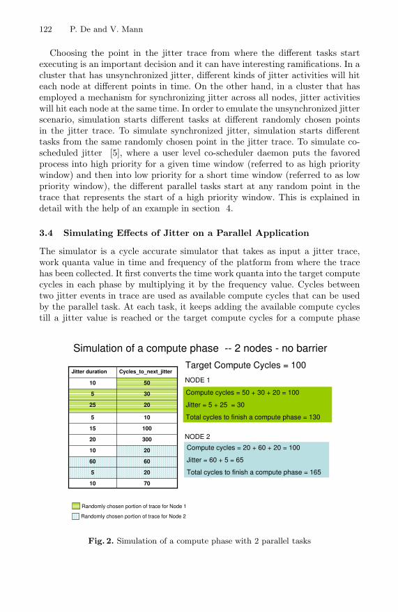
is reached. If a jitter value is reached, it is added to the total cycles consumed.When the target compute cycles are reached, it represents the end of a computephase and entry into the barrier phase. This is shown in Figure 2.
Due to jitter being introduced, different tasks will report a different value ofthe total cycles consumed in each phase, and maximum of all those values iscalculated to predict the overall completion time for that phase. The computetime taken by the faster tasks is subtracted from this maximum completion timeto calculate the number of cycles each task should wait (wasted cycles) beforestarting the next compute phase. This is shown in Figure 3.
After the end of N compute phases (N represents end of work or an experi-ment), an average of these overall completion times for each phase is calculated.Advantage of using a simulator approach is that one can use it to predict scala-bility at any processor count.
3.5 Simulating Effects of Co-scheduled or Synchronized Jitter on aParallel Application
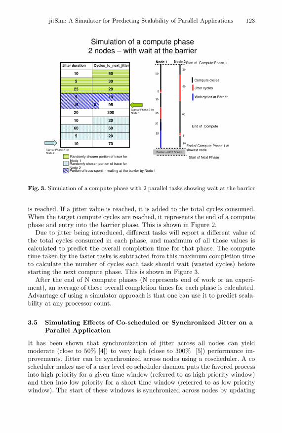
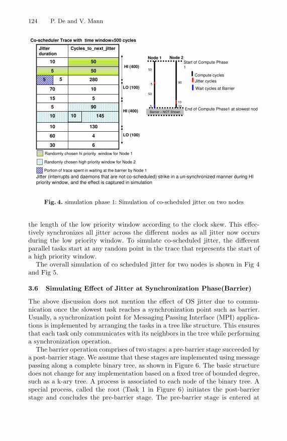
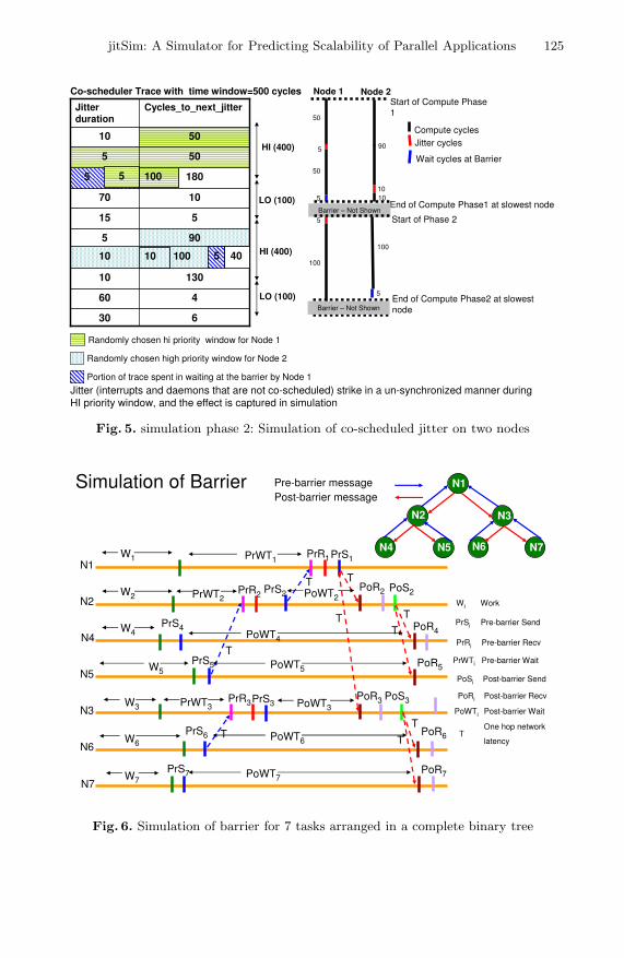
It has been shown that synchronization of jitter across all nodes can yieldmoderate (close to 50% [4]) to very high (close to 300% [5]) performance im-provements. Jitter can be synchronized across nodes using a coscheduler. A coscheduler makes use of a user level co scheduler daemon puts the favored processinto high priority for a given time window (referred to as high priority window)and then into low priority for a short time window (referred to as low prioritywindow). The start of these windows is synchronized across nodes by updating
124 P. De and V. Mann
Wait cycles at Barrier
5
Node 1 Node 2
630
460
13010
14510
905
515
1070
2805
505
5010
Cycles_to_next_jitterJitterduration
HI (400)
LO (100)
HI (400)
LO (100)
Jitter (interrupts and daemons that are not co-scheduled) strike in a un-synchronized manner during HIpriority window, and the effect is captured in simulation
End of Compute Phase1 at slowest nodBarrier – NOT Shown
Start of Compute Phase1
Compute cyclesJitter cycles
50
5
50
90
1010
10
Randomly chosen hi priority window for Node 1
Randomly chosen high priority window for Node 2
Portion of trace spent in waiting at the barrier by Node 1
5
Co-scheduler Trace with time window=500 cycles
Fig. 4. simulation phase 1: Simulation of co-scheduled jitter on two nodes
the length of the low priority window according to the clock skew. This effec-tively synchronizes all jitter across the different nodes as all jitter now occursduring the low priority window. To simulate co-scheduled jitter, the differentparallel tasks start at any random point in the trace that represents the start ofa high priority window.
The overall simulation of co scheduled jitter for two nodes is shown in Fig 4and Fig 5.
3.6 Simulating Effect of Jitter at Synchronization Phase(Barrier)
The above discussion does not mention the effect of OS jitter due to commu-nication once the slowest task reaches a synchronization point such as barrier.Usually, a synchronization point for Messaging Passing Interface (MPI) applica-tions is implemented by arranging the tasks in a tree like structure. This ensuresthat each task only communicates with its neighbors in the tree while performinga synchronization operation.
The barrier operation comprises of two stages: a pre-barrier stage succeeded bya post-barrier stage. We assume that these stages are implemented using messagepassing along a complete binary tree, as shown in Figure 6. The basic structuredoes not change for any implementation based on a fixed tree of bounded degree,such as a k-ary tree. A process is associated to each node of the binary tree. Aspecial process, called the root (Task 1 in Figure 6) initiates the post-barrierstage and concludes the pre-barrier stage. The pre-barrier stage is entered at
jitSim: A Simulator for Predicting Scalability of Parallel Applications 125
Node 1 Node 2
Wait cycles at Barrier
5
630
460
13010
10010
905
515
1070
1805
505
5010
Cycles_to_next_jitterJitterduration
HI (400)
LO (100)
HI (400)
LO (100)
Jitter (interrupts and daemons that are not co-scheduled) strike in a un-synchronized manner duringHI priority window, and the effect is captured in simulation
Randomly chosen hi priority window for Node 1
Randomly chosen high priority window for Node 2
Portion of trace spent in waiting at the barrier by Node 1
100
5 40
End of Compute Phase2 at slowestnode
100
5
100
Start of Phase 2
Barrier – Not Shown
5
End of Compute Phase1 at slowest nodeBarrier – Not Shown
Start of Compute Phase1
Compute cyclesJitter cycles
50
5
50
90
1010
10
Co-scheduler Trace with time window=500 cycles
5
Fig. 5. simulation phase 2: Simulation of co-scheduled jitter on two nodes
Simulation of Barrier N1
N2 N3
N4 N5 N6 N7
N7
N6
N3
N5
N4
N2
N1
Pre-barrier messagePost-barrier message
W1
W2
W4
W5
W3
W6
W7
PrS6
PrS7
PrR3PrWT3PrS3
PrS4
PrS5
T
T
PrR2 PrS2PrWT2
T
PrR1PrWT1 PrS1
T
PoWT4
PoR2 PoS2
PoR3 PoS3
T
T
TT
T
PoR4
PoR5
PoR6
PoR7
PoWT5
PoWT2
PoWT3
PoWT6
PoWT7
Wi
PrSi
Work
Pre-barrier Send
PrRi Pre-barrier Recv
PrWTi Pre-barrier Wait
PoSi Post-barrier Send
PoRi Post-barrier Recv
PoWTi Post-barrier Wait
TOne hop network
latency
Fig. 6. Simulation of barrier for 7 tasks arranged in a complete binary tree
126 P. De and V. Mann
the end of computation phase, when each task notifies its parents of completionof work. This stage ends when the root finishes its computation and receives amessage from both its children indicating the same. This is followed by a post-barrier stage, when a start-compute-phase message initiated by root is percolatedto all leaf nodes. A more complete description of the communication phase canbe found in [17].
Every time a message is sent from a task to its parent, or receives a messagefrom its children, certain number of cycles are allocated to that operation (andcounted as part of the compute cycles). These latencies are measured from theexperiments mentioned earlier. As the simulator traverses the trace, it looks forthe given number of send or receive cycles. If it encounters a jitter event duringthis time, the jitter cycles are added to the total cycles consumed. Simulation ofa barrier for 7 tasks arranged in a binary tree is shown in Figure 6.
4 Experimental Results
We conducted 3 main sets of experiments to prove the effectiveness of our jittersimulation methodology.
1. Validation of simulation results against real data2. Effect of length of trace on simulation3. Use of simulation results to evaluate various jitter mitigation techniques
All results in this section assume a 1 to 1 correspondence between Processorsand MPI tasks. For example, a result at 16K Processor implies that there are16K MPI tasks that are running on 16K Processors, each with its own OS image.
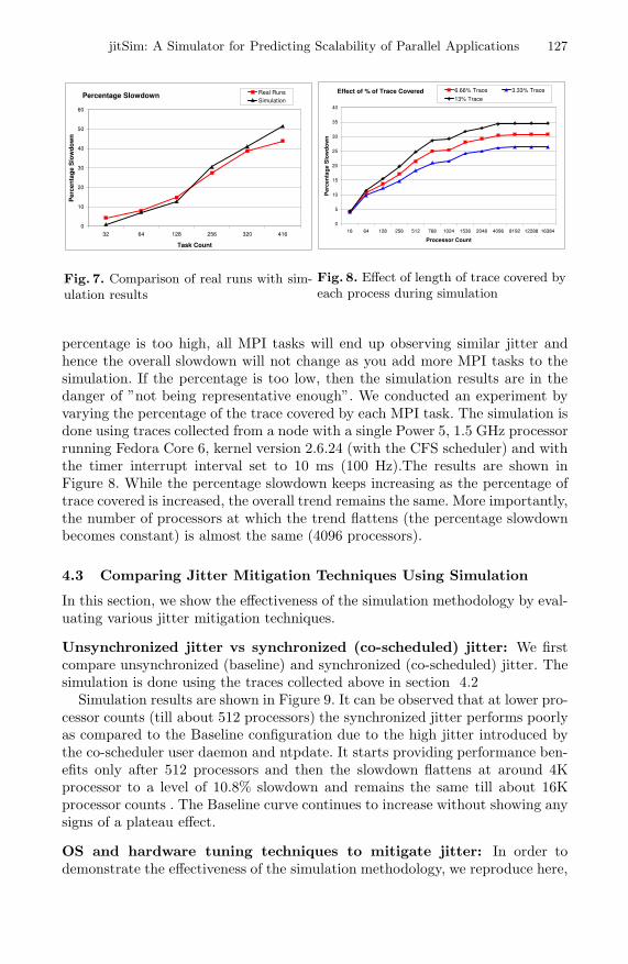
4.1 Comparing Simulator Results with Real Runs
A comparison of scalability prediction from simulation with real runs on Linuxrunning in run level 3 in the baseline (unsynchronized jitter) version is given inFigure 7. The real runs were done on a cluster with 13 identical nodes and eachnode had 32 Power6 cores running SLES 10. For simulation, a trace was collectedfrom each of the 32 cores on a node. Scalability prediction from simulationmatches the real results closely. In this case, simulation used only the averagemaximum compute times (i.e. the compute phase and the wait after the computephase due to synchronization point) and did not include the slowdown in thecommunication phase.
4.2 Effect of Trace Coverage by Each Process during Simulation
One of the critical factors that controls the accuracy of the simulation processis the overall length of the trace used for simulation and what percentage ofit gets covered by each MPI task. We found that a jitter trace of about anhour was sufficient to capture most periodic daemons. The percentage of thetrace covered by each MPI task is a more difficult parameter to decide. If the
jitSim: A Simulator for Predicting Scalability of Parallel Applications 127
Percentage Slowdown
0
10
20
30
40
50
60
32 64 128 256 320 416
Task Count
Per
cen
tag
eS
low
do
wn
Real RunsSimulation
Fig. 7. Comparison of real runs with sim-ulation results
Effect of % of Trace Covered
0
5
10
15
20
25
30
35
40
16 64 128 256 512 768 1024 1536 2048 4096 8192 12288 16384
Processor Count
Per
cen
tag
eS
low
do
wn
6.66% Trace 3.33% Trace
13% Trace
Fig. 8. Effect of length of trace covered byeach process during simulation
percentage is too high, all MPI tasks will end up observing similar jitter andhence the overall slowdown will not change as you add more MPI tasks to thesimulation. If the percentage is too low, then the simulation results are in thedanger of ”not being representative enough”. We conducted an experiment byvarying the percentage of the trace covered by each MPI task. The simulation isdone using traces collected from a node with a single Power 5, 1.5 GHz processorrunning Fedora Core 6, kernel version 2.6.24 (with the CFS scheduler) and withthe timer interrupt interval set to 10 ms (100 Hz).The results are shown inFigure 8. While the percentage slowdown keeps increasing as the percentage oftrace covered is increased, the overall trend remains the same. More importantly,the number of processors at which the trend flattens (the percentage slowdownbecomes constant) is almost the same (4096 processors).
4.3 Comparing Jitter Mitigation Techniques Using Simulation
In this section, we show the effectiveness of the simulation methodology by eval-uating various jitter mitigation techniques.
Unsynchronized jitter vs synchronized (co-scheduled) jitter: We firstcompare unsynchronized (baseline) and synchronized (co-scheduled) jitter. Thesimulation is done using the traces collected above in section 4.2
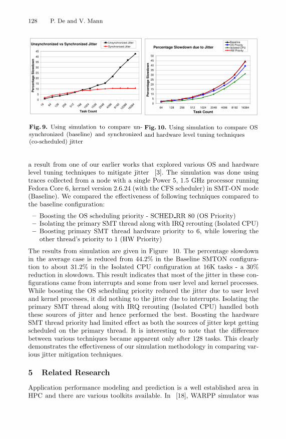
Simulation results are shown in Figure 9. It can be observed that at lower pro-cessor counts (till about 512 processors) the synchronized jitter performs poorlyas compared to the Baseline configuration due to the high jitter introduced bythe co-scheduler user daemon and ntpdate. It starts providing performance ben-efits only after 512 processors and then the slowdown flattens at around 4Kprocessor to a level of 10.8% slowdown and remains the same till about 16Kprocessor counts . The Baseline curve continues to increase without showing anysigns of a plateau effect.
OS and hardware tuning techniques to mitigate jitter: In order todemonstrate the effectiveness of the simulation methodology, we reproduce here,
128 P. De and V. Mann
Unsynchronized vs Synchronized Jitter
0
5
10
15
20
25
30
35
40
45
16 64 128
256
512
768
1024
1536
2048
4096
8192
1228
8
1638
4
Task Count
Per
cen
tag
eS
low
do
wn
Unsynchronized JitterSynchronized Jitter
Fig. 9. Using simulation to compare un-synchronized (baseline) and synchronized(co-scheduled) jitter
Percentage Slowdown due to Jitter
0
5
10
15
20
25
30
35
40
45
50
64 128 256 512 1024 2048 4096 8192 16384
Task Count
Per
cen
tag
eS
low
do
wn
BaselineOS PriorityIsolated CPUHW Priority
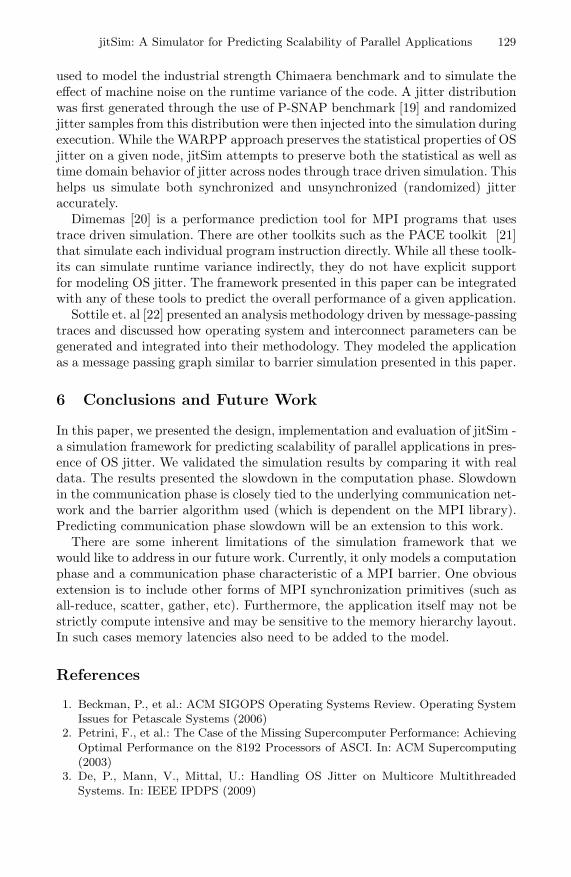
Fig. 10. Using simulation to compare OSand hardware level tuning techniques
a result from one of our earlier works that explored various OS and hardwarelevel tuning techniques to mitigate jitter [3]. The simulation was done usingtraces collected from a node with a single Power 5, 1.5 GHz processor runningFedora Core 6, kernel version 2.6.24 (with the CFS scheduler) in SMT-ON mode(Baseline). We compared the effectiveness of following techniques compared tothe baseline configuration:
– Boosting the OS scheduling priority - SCHED RR 80 (OS Priority)– Isolating the primary SMT thread along with IRQ rerouting (Isolated CPU)– Boosting primary SMT thread hardware priority to 6, while lowering the
other thread’s priority to 1 (HW Priority)
The results from simulation are given in Figure 10. The percentage slowdownin the average case is reduced from 44.2% in the Baseline SMTON configura-tion to about 31.2% in the Isolated CPU configuration at 16K tasks - a 30%reduction in slowdown. This result indicates that most of the jitter in these con-figurations came from interrupts and some from user level and kernel processes.While boosting the OS scheduling priority reduced the jitter due to user leveland kernel processes, it did nothing to the jitter due to interrupts. Isolating theprimary SMT thread along with IRQ rerouting (Isolated CPU) handled boththese sources of jitter and hence performed the best. Boosting the hardwareSMT thread priority had limited effect as both the sources of jitter kept gettingscheduled on the primary thread. It is interesting to note that the differencebetween various techniques became apparent only after 128 tasks. This clearlydemonstrates the effectiveness of our simulation methodology in comparing var-ious jitter mitigation techniques.
5 Related Research
Application performance modeling and prediction is a well established area inHPC and there are various toolkits available. In [18], WARPP simulator was
jitSim: A Simulator for Predicting Scalability of Parallel Applications 129
used to model the industrial strength Chimaera benchmark and to simulate theeffect of machine noise on the runtime variance of the code. A jitter distributionwas first generated through the use of P-SNAP benchmark [19] and randomizedjitter samples from this distribution were then injected into the simulation duringexecution. While the WARPP approach preserves the statistical properties of OSjitter on a given node, jitSim attempts to preserve both the statistical as well astime domain behavior of jitter across nodes through trace driven simulation. Thishelps us simulate both synchronized and unsynchronized (randomized) jitteraccurately.
Dimemas [20] is a performance prediction tool for MPI programs that usestrace driven simulation. There are other toolkits such as the PACE toolkit [21]that simulate each individual program instruction directly. While all these toolk-its can simulate runtime variance indirectly, they do not have explicit supportfor modeling OS jitter. The framework presented in this paper can be integratedwith any of these tools to predict the overall performance of a given application.
Sottile et. al [22] presented an analysis methodology driven by message-passingtraces and discussed how operating system and interconnect parameters can begenerated and integrated into their methodology. They modeled the applicationas a message passing graph similar to barrier simulation presented in this paper.
6 Conclusions and Future Work
In this paper, we presented the design, implementation and evaluation of jitSim -a simulation framework for predicting scalability of parallel applications in pres-ence of OS jitter. We validated the simulation results by comparing it with realdata. The results presented the slowdown in the computation phase. Slowdownin the communication phase is closely tied to the underlying communication net-work and the barrier algorithm used (which is dependent on the MPI library).Predicting communication phase slowdown will be an extension to this work.
There are some inherent limitations of the simulation framework that wewould like to address in our future work. Currently, it only models a computationphase and a communication phase characteristic of a MPI barrier. One obviousextension is to include other forms of MPI synchronization primitives (such asall-reduce, scatter, gather, etc). Furthermore, the application itself may not bestrictly compute intensive and may be sensitive to the memory hierarchy layout.In such cases memory latencies also need to be added to the model.
References
1. Beckman, P., et al.: ACM SIGOPS Operating Systems Review. Operating SystemIssues for Petascale Systems (2006)
2. Petrini, F., et al.: The Case of the Missing Supercomputer Performance: AchievingOptimal Performance on the 8192 Processors of ASCI. In: ACM Supercomputing(2003)
3. De, P., Mann, V., Mittal, U.: Handling OS Jitter on Multicore MultithreadedSystems. In: IEEE IPDPS (2009)
130 P. De and V. Mann
4. Terry, P., Shan, A., Huttunen, P.: Improving application performance on HPCsystems with process synchronization. Linux Journal (127), 68–73 (November 2004)
5. Jones, T., et al.: Improving the scalability of parallel jobs by adding parallel aware-ness to the operating system. In: ACM Supercomputing (2003)
6. ZeptoOS: The small linux for big computers,http://www-unix.mcs.anl.gov/zeptoos/
7. Team, T.B.G.: An Overview of the Blue Gene/L Supercomputer. In: ACM Super-computing (2002)
8. CrayXT5: Cray XT5 Supercomputer,http://www.cray.com/Products/XT/Systems/XT5.aspx
9. MareNostrum: Barcelona Supercomputing Center, http://www.bsc.es/10. Hoisie, A., et al.: A Performance Comparison through Benchmarking and Modeling
of Three Leading Supercomputers: Blue Gene/L, Red Storm, and Purple. In: ACMSupercomputing (2006)
11. Ferreira, K., Bridges, P., Brightwell, R.: Characterizing application sensitivity toOS interference using kernel-level noise injection. In: ACM Supercomputing (2008)
12. Right-weight Linux Kernel Project: Los Alamos National Laboratory,http://public.lanl.gov/cluster/projects/index.html
13. Kaplan, L.S.: Lightweight Linux for High-Performance Computing. Linux-World.com (December 2006)
14. De, P., Kothari, R., Mann, V.: A Trace-driven Emulation Framework to PredictScalability of Large Clusters in Presence of OS Jitter. In: IEEE Cluster (2008)
15. Beckman, P., et al.: The Influence of Operating Systems on the Performance ofCollective Operations at Extreme Scale. In: IEEE Cluster Computing (2006)
16. De, P., Kothari, R., Mann, V.: Identifying Sources of Operating System JitterThrough Fine-Grained Kernel Instrumentation. In: IEEE Cluster (2007)
17. De, P., Garg, R.: The Impact of Noise on the Scaling of Collectives: An EmpiricalEvaluation. In: Robert, Y., Parashar, M., Badrinath, R., Prasanna, V.K. (eds.)HiPC 2006. LNCS, vol. 4297. Springer, Heidelberg (2006)
18. Hammond, S., et al.: WARPP: a toolkit for simulating high-performance parallelscientific codes. In: International Conference on Simulation Tools and Techniques(2009)
19. P-SNAP Benchmark: P-SNAP Benchmark,http://www.ccs3.lanl.gov/pal/software/psnap/
20. Girona, S., Labarta, J.: Sensitivity of Performance Prediction of Message Pass-ing Programs. In: International Conference on Parallel and Distributed ProcessingTechniques and Applications (1999)
21. Nudd, et al: PACE: A Toolset for the Performance Prediction of Parallel andDistributed Systems. The International Journal of High Performance Computing(2000)
22. Sottile, M., Chandu, V., Bader, D.: Performance analysis of parallel programs viamessage-passing graph traversal. In: IEEE IPDPS (2006)