Computational Methods in Molecular and Cellular Biology: from Genotype to Phenotype.J.M. Bower and H. Bolouri editorsMIT Press, Boston Reviews in the Neurosciences

Chapter 8: Modeling molecular diffusion

G.Bormann1, F. Brosens2, E. De Schutter1

1Born-Bunge Foundation, University of Antwerp - UIA, B2610 Antwerp, Belgium 2Dept. of Physics, University of Antwerp - UIA, B2610 Antwerp, Belgium

1 Introduction

1.1 Why model diffusion in cells?

Physical proximity is an essential requirement for molecular interaction to occur, whether it isbetween an enzyme and its substrate and modulators or between a receptor and its ligand. Cellshave developed many mechanisms to bring molecules together, including structural ones, e.g.calcium-activated ionic channels often cluster with calcium channels in the plasma membrane(Gola and Crest, 1993; Issa and Hudspeth, 1994), or specific processes like active transport (Nixon,1998). In many situations, however, concentration gradients exist which will affect the local rate ofchemical reactions. Such gradients can be static at the timescale of interest, e.g. the polarity of cells(Kasai and Petersen, 1994), or very dynamic like for example the intra- and intercellular signalingby traveling calcium waves (Berridge, 1997).

Diffusion is the process by which random Brownian movement of molecules or ions cause anaverage movement towards regions of lower concentration, which may result in the collapse of theconcentration gradient. In the context of cellular models, one distinguishes-experimentally andfunctionally-between free diffusion and diffusion across or inside cell membranes (Hille, 1992).We will only consider the first case explicitly, but similar methods as described here can be appliedto the latter.

Historically, diffusion has often been neglected in molecular simulations which are then assumedto operate in ’the well-mixed pool’. This assumption may be valid when modeling small volumes,e.g. inside a spine (Koch and Zador, 1993), but should be carefully evaluated in all other contexts.As we will see in this chapter, the introduction of diffusion into a model raises many issues whichotherwise do not apply: spatial scale, dimensionality, geometry and which individual molecules orions can be considered to be immobile or not. The need for modeling diffusion should be evaluatedfor each substance separately. In general, if concentration gradients exist within the spatial scale ofinterest it is highly likely that diffusion will have an impact on the modeling results, unless thegradients change so slowly that they can be considered stationary compared to the timescale ofinterest.

Simulating diffusion is in general a computationally expensive decision which is a more practicalexplanation of why it is often not implemented. This may very well change in the near future. Agrowing number of modeling studies (Markram et al., 1998; Naraghi and Neher, 1997) have recently emphasised the important effects diffusion can have on molecular interactions.

1.2 When is diffusion likely to make a difference?

A reaction-diffusion system is classically described as one where binding reactions are fast enoughto affect the diffusion rate of the molecule or ion of interest (Wagner and Keizer, 1994; Zador andKoch, 1994). A classic example which we will consider is the interaction of calcium withintracellular buffers, which cause calcium ions to spread ten times slower than one would expectfrom the calcium diffusion constant (Kasai and Petersen, 1994).

Depending on which region of the cell one wants to model, this slow effective diffusion can begood or bad news. In fact, the slow effective diffusion rate will dampen rapid changes caused bycalcium influx through a plasma membrane so much that in the center of the cell it can be modeledas a slowly changing concentration without gradient. Conversely, below the plasma membrane theslower changes in concentration gradient may need to be taken into full account (fig.3C).

This is, however, a static analysis of the problem while the dynamics of the reaction-diffusionprocess may be much more relevant to the domain of molecular interactions. In effect, as we willdiscuss in some detail, binding sites with different affinities may compete for the diffusingmolecule which leads to highly nonlinear dynamics. This may be a way for cells to spatiallyorganise chemical reactions in a deceptively homogenous intracellular environment (Markram et al., 1998; Naraghi and Neher, 1997).

Before dealing with reaction-diffusion systems, however, we will consider the diffusion processitself in some detail. In this context we will consider especially those conditions under which thestandard one-dimensional diffusion equation description used in most models is expected to fail.

2 Characteristics of diffusion systems.

Part I provided a concise introduction to the modeling of chemical kinetics based on mass action,expressed as reaction rate equations. It also discussed the shortcomings of the rate equationapproach for describing certain features of chemical reactions and provided alternatives, e.g.Markov processes, to improve models of chemical kinetics.

These improvements stem from the realisation that under certain circumstances the stochasticnature of molecular interactions can have a profound effect on the dynamical properties. Theresulting models still share a common assumption with rate equation models in that they assume awell-mixed homogenous system of interacting molecules. This ignores the fact that spatialfluctuations may introduce yet another influence on the dynamics of the system. For example, inmany cases it is important to know how a spatially localised disturbance can propagate in thesystem.

From statistical mechanics it follows that adding spatial dependence to the molecule distributionscalls for a transport mechanism which dissipates gradients in the distribution. This mechanism iscalled diffusion and it is of a statistical nature. The effects on the dynamics of the chemical systemare determined by the relative timescales of the diffusion process and the chemical kineticsinvolved.

At the end of this section we will describe a number of examples of how diffusion interacts with achemical system thereby creating new dynamics. First, however, we will consider diffusion byitself as an important and relatively fast transport mechanism in certain systems. We will alsodiscuss how to relate diffusion to experimental data and show that such data mostly provide awarped view on diffusion. Therefore it is usually more appropriate to talk about ’apparentdiffusion’. The appearance of this apparent diffusion, i.e. the degree of warpedness compared tofree diffusion, is determined both by the nature of the chemical reactions and by the specific spatialgeometry of the system under investigation.

This chapter provides methods of different nature to solve the equations that govern thesephenomena and will give guidelines concerning their applicability. This should enable the reader tomake initial guesses about the importance of diffusion in the system under consideration, whichcan help decide whether or not to pursue a more detailed study of the full reaction-diffusionsystem.

2.1 What is diffusion?

Diffusional behaviour is based on the assumption that the molecules perform a random walk in thespace that is available to them. This is called Brownian motion. The nature of this random walk issuch that the molecules have equal chance to go either way (in the absence of external fields). Tosee how this can generate a macroscopic effect (as described by Fick’s law, see later) let’s considera volume element in which there are more molecules than in a neighbouring volume element.Although the molecules in both volume elements have equal chance of going either way, there aremore molecules that happen to go to the element with the low initial number of molecules thanthere are molecules coming to the high initial number element because they simply outnumberthem.

To describe this process mathematically we assume the molecules perform a discrete random walkby forcing them to take a step of fixed length x in a random direction (i.e. left or right) every fixed t, independent of previous steps. The average change in number of molecules n

ik at

discrete position i in a timestep t from tk to t

k+1 for a high enough number of molecules is then

given by (see for instance (Schulman, 1981))

( 1 )

where pl and p

r are the probabilities to go either to the left or to the right. In the absence of drift we

have for the probabilities (using the sum rule for independent events)

( 2 )

so that

Filling in these numbers in eq.(1) gives

( 3 )

resulting in

( 4 )

Letting x->0 and t->0 while keeping

( 5 )

constant (and multiplying both sides with a constant involving Avogadro’s number(6.022*1023mol-1) and volume to convert to concentrations), we get the following parabolic PDE:[1]

( 6 )

This is generally known as the one-dimensional diffusion equation along a Cartesian axis. Otherone-dimensional equations are used more often but they arise from symmetries in amulti-dimensional formulation, e.g. the radial component in a spherical or cylindrical coordinatesystem (see below). The random walk can be easily extended to more dimensions by using thesame update scheme for every additional (Cartesian) coordinate.

The random walk process described above generates a Gaussian distribution of molecules over allgrid positions when all molecules start from a single grid position x

0 (i.e. a Dirac delta function) :

( 7 )

It’s left as an exercise for the reader to proof this [2]. From this, and the fact that every function can be written as a series of delta functions, it follows that the same solution can be generated using a continuous random walk by drawing the step size each molecule moves every timestep t from aGaussian of the form

( 8 )

which has a mean square step size of ( x)2=2D t , relating the two random walk methods. The

choice of the method to use is determined by the following : discrete random walks allow a fast evaluation of the local density of molecules while continuous random walks allow easy inclusion [3] of complex boundary conditions.

The above is a quick way to determine the solution of eq.(6) for the initial condition [4] C(x,0)=C0

(x-x0). This is one of the few cases that can also be solved analytically. See Crank (Crank, 1975)

for a general and extensive analytical treatment of the diffusion equation.

Fig. 1: The initial condition is the distribution of molecules on a fixed time t (chosen as t=0 in most cases). It determines the final shape of thedistribution at a later time t+T. In general, a partial differential equation (in space and time) has a set ofpossible solutions for a fixed set of parameters and(spatial) boundary conditions. By setting the initial condition, one selects a specific solution.

A final remark concerning the scale on which the random walk approach applies should be made.The movements the molecules make in the diffusion process are related to the thermal movementof and collisions with the background solvent molecules. The path a single molecule follows iserratic but each step is deterministic when the molecules are considered to be hard spheres. If theenvironment of the molecule is random though, the resulting path can be considered the result of arandom walk where each step is independent of the molecule’s history(Hille, 1992).

Nevertheless, even in a fluid the close range environment of a molecule has some short termsymmetry in the arrangement of the surrounding molecules so that on the scale of the mean freepath (and the corresponding pico/femto second time scale) there is some correlation in the steps ofthe molecule-i.e. the molecule appears to be trapped in its environment for a short time. At thisscale using random walks is not appropriate and one has to resort to Molecular Dynamics instead.At a larger distance (and thus at a longer timescale), the environment appears random again in afluid and the correlations disappear so that a random walk approach is valid again.

2.2 A macroscopic description of diffusion.

Many discussions about diffusion start out with an empirical law : Fick’s law (Fick, 1885). Thislaw states that a concentration gradient for a dissolved substance gives rise to a flux of mass in the(diluted) solution, proportional to but in the opposite direction of the concentration gradient. Theconstant of proportionality is called the (macroscopic) diffusion constant. It is valid under quitegeneral assumptions. The corresponding equation in one dimension is of the form

( 9 )

where D is the macroscopic diffusion constant and C(x,t) is the mass distribution functionexpressed as a concentration. The minus sign is there to ensure that the mass will flow downhill onthe concentration gradient (otherwise we get an unstable system and the thermodynamic law ofentropy would be violated).

The diffusion constant is usually treated as a fundamental constant of nature for the species athand, determined from diffusion experiments. It is, however, not a real fundamental constant sinceit can be calculated, using kinetic gas theory, from thermodynamic constants, absolute temperatureand molecule parameters. In fact, it can even be position-dependent if the properties of the medium(like the viscosity) vary strongly with position. So, including diffusion in an accurate model couldbecome a messy business in some cases.

Fick’s law looks very much like an expression for a flux proportional to a conservative force on themolecules, with the ’force’ depending on the gradient of a field potential (the concentration). But,as can be concluded from section 5, that ’force’ is entirely of a statistical nature. The flux of masschanges the concentration at all points of nonzero net flux. The rate of change is given by a massbalance (i.e. a continuity) equation as follows

( 10 )

in the absence of other nonFickian fluxes. Replacing JF(x,t) by the right-hand side of eq.(9) gives

eq.(4) if we identify the diffusion constant with the former constant D. For more details on kineticgas theory and a derivation of this macroscopic diffusion constant from microscopicconsiderations, see for example The Feynman Lectures (Feynman et al., 1989). A classic is ofcourse Einstein’s original treatment of Brownian motion (Einstein, 1905).

Eqs.(9) and (10) can be easily extended to higher dimensions by using the following vectornotations

( 11 )

where " " is the gradient operator and " " the divergence operator. Combining the twoequations then gives the general multi-dimensional diffusion equation

( 12 )

with the Laplace operator (Laplacian). The explicit form of the Laplacian depends on the chosen coordinate system. In a Cartesian system in ordinary space it looks like this

( 13 )

Sometimes the nature of the problem is such that it is simpler to state the problem in cylindrical [5]

( 14 )

or spherical [6] coordinates

( 15 )

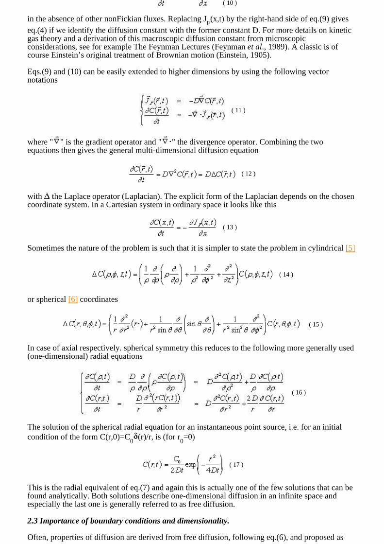
In case of axial respectively. spherical symmetry this reduces to the following more generally used(one-dimensional) radial equations

( 16 )

The solution of the spherical radial equation for an instantaneous point source, i.e. for an initialcondition of the form C(r,0)=C

0(r)/r, is (for r

0=0)

( 17 )

This is the radial equivalent of eq.(7) and again this is actually one of the few solutions that can befound analytically. Both solutions describe one-dimensional diffusion in an infinite space andespecially the last one is generally referred to as free diffusion.

2.3 Importance of boundary conditions and dimensionality.

Often, properties of diffusion are derived from free diffusion, following eq.(6), and proposed as

generic diffusion properties while the actual boundary conditions shape the concentration profilesin significantly different ways. Knowing these shapes can be important when interpretingexperimental results or when selecting curves-i.e. solutions of model problems-for fittingexperimental data to estimate (apparent) diffusion parameters.

Choosing the appropriate boundary conditions is also important from a modeling point of view.Free diffusion is of use to model interactions in infinite space or in a bulk volume on appropriatetimescales, i.e. situations where diffusion is used as a simple passive transport or dissipativemechanism. However, when diffusion is used as a transport mechanism to link cascading processesthat are spatially separated or when diffusion is used in conjunction with processes that aretriggered at certain concentration level thresholds, a detailed description of the geometry of thesystem may become very important. In that case the complex geometry can impose the majority ofthe boundary conditions.

To give an example, let’s consider a cylinder of infinite length, with a reflecting mantle, in whichthere is an instantaneous point source releasing a fixed amount of substance A while further downthe cylinder there is a store of another substance B. The store starts releasing substance B when theconcentration of substance A reaches a certain threshold level. For smaller radii of the cylinder thetime of release from the store will be much shorter. This is because the concentration of A at thestore will rise sooner to the threshold level for smaller radii, although the intrinsic diffusion rate ofA does not change.

When the concentration level of A has to be sustained for a longer period, consider what happenswhen we seal off the cylinder with a reflecting wall near the point source. Since mass can now onlyspread in one general direction, the concentration of A can become almost twice as high ascompared to the unsealed case, the exact factor depending on the distance between the point sourceand the sealed end. Furthermore, the concentration near the store and point source will stayelevated for a longer period of time. Eventually, the concentration will drop to zero in this casesince the cylinder is still semi-infinite. When we seal off the other end too (at a much largerdistance), then the concentration of A will, not surprisingly, drop to a fixed rest level-above orbelow the threshold level, depending just on the volume of the now finite closed cylinder-when noremoval processes are present.

Boundary conditions play also a major role in the dimensionality of the diffusion equation one hasto choose. Eqs.(16) are examples of equations that arise from certain symmetries in the boundaryconditions. Often the dimensionality is also reduced by neglecting asymmetries in somecomponents of the boundary conditions or by averaging them out for these components in order toreduce computation time or computational complexity. In some cases, though, it is necessary tokeep the full dimensionality of the problem to be able to give an accurate description of the system.This is for example the case in cell models where compartmentalization is obtained through spatialco-localization of related processes. In order to simulate such models, one has to resort to fastmulti-dimensional numerical methods. The methods section provides two such methods: one finitedifferencing method called ADI and one Monte Carlo method called Green’s Function MonteCarlo.

2.4 Interactions among molecules and with external fields.

In the reaction rate equation approach a system of chemical reactions can be described in generalby a set of coupled first-order ODE’s:

( 18 )

where the form of the functions fs are determined by the reaction constants and structures of the M

chemical reaction channels. The functions fs are generally nonlinear in the C

s’s. In case the

reaction mechanisms and constants are known, one can use the following normal form for the fs’s:

( 19 )

with , where the are the stoichiometric coefficients for substance s on

the left-hand respectively right-hand side of the reaction equation for reaction c [7] and kc is the

reaction constant. Most of the are zero. is known as the reaction order and is related to the order of the collisions between the reacting molecules. Since collisions of order higher than 4 are extremely improbable, R

c 4 for most reactions. A reaction of higher order

is most likely a chain of elementary reaction steps.

Combining the rate equations with a set of diffusion equations now results in a set of couplednonlinear parabolic PDE’s :

( 20 )

The first term of the right-hand side will be 0 for all immobile substances. Systems governed by aset of equations like eqs.(18) can exhibit a broad array of complex temporal patterns. Including atransport mechanism to introduce spatial dependence as described by eqs.(20) can introduceadditional complex spatial patterns.

Only very simple cases can be solved analytically for both types of problems, so one has to resortto numerical methods which can become very involved for the second type of problems. At lowmolecule densities, classic integration methods like the ones introduced in section 14 cannot graspthe full dynamics of the system because they don’t include the intrinsic fluctuations. One has toresort to stochastic approaches for the chemical kinetics like the ones introduced in Part I and forthe diffusion like the Monte Carlo method introduced in the Numerical Methods section.

Reaction partners can be electrically charged. Although this can have an important influence on thereaction kinetics, it is usually handled by adjusting the rate constants (in case of rate models) or thereaction probabilities (in case of stochastic models). However, one can think of problems where it’simportant to know the effects of local or external electric fields on diffusion. One can start studyingthese problems by rewriting eqs.(11) to

( 21 )

where is the net flux induced by the Coulomb interactions between the charged molecules and the net flux induced by the interaction of the charged molecules with an external field of

potential V. z is the valence of the ionic species, F is the Faraday constant, R is the gas constant and T is absolute temperature. The second equation is called the electrodiffusion equation. In the case of , it is called the Nernst-Plank equation (Hille, 1992). Special complicated numerical

algorithms have to be used to solve the general electrodiffusion equation because of the long rangeand the 1/r divergence of Coulomb interactions. For an application to synaptic integration indendritic spines, see for example Qian and Sejnowski (Qian and Sejnowski, 1990).

2.5 An example of reaction-diffusion systems: calcium buffering in the cytoplasm.

Reaction-diffusion systems have been studied most extensively in the context of buffering andbinding of calcium ions. Calcium is probably the most important intracellular signaling molecule.Its resting concentration is quite low (about 50 nM) but it can raise by several orders of magnitude(up to 100’s of M’s) beneath the pore of calcium channels (Llinás et al., 1992). Cells contain an impressive variety of molecules with calcium binding sites, this includes pumps which remove the calcium (e.g. the calcium-ATPase;(Garrahan and Rega, 1990)), buffers which bind the calcium (e.g. calbindin, calsequestrin, calretinin, etc.;(Baimbridge et al., 1992)), enzymes activated by calcium (for example phospholipases;(Exton, 1997)) or modulated by calcium (for example through calmodulin activation;(Farnsworth et al., 1995)). The interaction of the transient steepcalcium concentration gradients with all these binding sites creates complex reaction-diffusionsystems, the properties of which are not always completely understood. For example, it remains apoint of discussion whether calcium waves, which are caused by inositol1,4,5-triphosphate (IP

3)

activated release of calcium from intracellular stores, propagate because of diffusion of IP3

(Bezprozvanny, 1994; Sneyd et al., 1995) itself or of calcium (Jafri and Keizer, 1995), which has a complex modulatory effect on the IP

3 receptor (Bezprozvanny et al., 1991).

We will focus on the macroscopic interaction of calcium with buffer molecules. The main functionof buffers is to keep the calcium concentration within physiological bounds by binding most of thefree calcium. Almost all models of the interactions of calcium with buffers use the simplesecond-order equation:

( 22 )

Eq.(22) is only an approximation as most buffer molecules have multiple binding sites withdifferent binding rates (Linse et al., 1991) and require more complex reaction schemes (see first section of this book). In practice, however, experimental data for these different binding rates are often not available. Nevertheless, it is important to express buffer binding with rate equations, evensimplified ones, instead of assuming the binding reactions to be in steady-state, described by thebuffer dissociation constant K

d=b/f like is often done (e.g. (Goldbeter et al., 1990; Sneyd et al.,

1994)). Even if the time scale of interest would allow for equilibrium to occur, the use of steady-state equations neglects the important effects of the forward binding rate constant f on diffusion and competition between buffers (see further).

Fig. 2: A pictorial description of the effect of buffer binding on calcium diffusion for slowly diffusing buffers. The yellow dots represent calcium ions, the green blobs buffer molecules, the purple blobs are calcium channels and the lightning symbol represents chemical interaction. The reacting dot

is gradient-colored to distinguish it from the other intracellular dot. Note that the figure only shows the net effect for the respective populations. In reality, individual molecules follow erratic pathsthat don’ t directly show the buffering effect.

While the properties of buffered calcium diffusion have been mostly studied using analyticalapproaches (Naraghi and Neher, 1997; Wagner and Keizer, 1994; Zador and Koch, 1994), it isfairly simple to demonstrate these concepts through simulation of the system corresponding to theset of differential equations described in the next section (see also (Nowycky and Pinter, 1993) fora similar analysis). The simulations of the simple models that [8] we used were run with the GENESIS software (the simulation scripts can be downloaded from the Webhttp://www.bbf.uia.ac.be/models/models.shtml). For more information on simulating calciumdiffusion with the GENESIS software (Bower and Beeman, 1995) we refer to De Schutter and Smolen (De Schutter and Smolen, 1998). We will focus on the transient behavior of thereaction-diffusion system, i.e. the response to a short pulsatile influx of calcium through the plasma membrane. Also, as we are interested mostly in molecular reactions we will stay in the nonsaturated regime [Ca2+]<<K

d) though of course interesting nonlinear effects can be obtained

when some buffers start to saturate. Finally, for simplicity we do not include any calcium removalmechanisms (calcium pumps ;(Garrahan and Rega, 1990) and the Na+Ca2+ exchanger;(DiFrancesco and Noble, 1985)), though they are expected to have important additional effects bylimiting the spread of the calcium transients (Markram et al., 1998; Zador and Koch, 1994).

The diffusion constant of calcium (DCa

) in water is 6*10-6cm2s-1. In cytoplasm, however, the measured diffusion constant is much lower because of the high viscosity of this medium. Albritton et al.(Albritton et al., 1992) measured a D

Ca of 2.3*10-6cm2s-1 in cytoplasm and other ions and

small molecules can be expected to be slowed down by the same factor. As shown in fig.3A, with this D

Ca calcium rises rapidly everywhere in a typical cell, with only a short delay of about 10 ms

in the deepest regions. After the end of the calcium influx, the calcium concentration reaches equilibrium throughout the cell in less than 200 ms. Down to about 3.0 m the peak calcium concentration is higher than the equilibrium one because influx rates are higher than the rate of removal by diffusion.

Fig. 3: Effect of immobile buffer binding rates on calcium diffusion. Thechanges in calcium concentration at several distances from the plasma membrane) due to a short calciumcurrent into a spherical cell are shown.

A Calcium concentration for simulation with no buffers present.

B Same with buffer with slow forward rate f (similar to EGTA) present.

C Same with buffer with fast f (similar to BAPTA) present. Fainter colors:approximation using D

app (eq.(24)).

D Bound buffer concentration for simulation shown in B

E Same for simulation shown in C

This diffusion constant is attained only if no binding to buffers occurs (Albritton et al.(Albritton et al., 1992)) completely saturated the endogenous buffers with calcium to obtain their measurements). Figs.3(B-E) demonstrates the effect of stationary buffers on the effective calciumdiffusion rate: they decrease both the peak and equilibrium calcium concentration, slow thediffusion process down and limit the spread of calcium to the submembrane region (i.e. close to thesite of influx). The total buffer concentration [B]

T=[B]+[CaB] and its affinity, which is high in

these simulations (Kd=0.2 M), will determine the amount of free calcium at equilibrium. This is

called the buffer capacity of the system, which is also the ratio of the inflowing ions that are boundto buffer to those that remain free (Augustine et al., 1985; Wagner and Keizer, 1994) :

( 23 )

In case of low calcium concentration eq.(23) reduces to [B]T/K

d. Buffer capacities in the cytoplasm

are high, ranging from about 45 in adrenal chromaffin cells (Zhou and Neher, 1993) to more than4000 in Purkinje cells (Llano et al., 1994).

While the buffer capacity determines the steady-state properties of the system, the dynamics arehighly dependent on the forward binding rate f (compare fig.3B with fig.3C). In effect, for the

same amount of buffer and the same high affinity the calcium profiles are very different. For theslow buffer as in fig.3B, calcium rises rapidly everywhere in the cell with similar delays as infig.3A, but reaches much lower peak concentrations. Only about 50% of the buffer gets boundbelow the plasma membrane. After the end of the calcium influx the decay to equilibrium has avery rapid phase, comparable to that in fig.3A, followed by a much slower relaxation which takesseconds. The peak calcium concentrations are comparatively much higher than the equilibriumconcentration of 95 nM down to a depth of 5.0 m. Note the slow relaxation to equilibrium of bound buffer in fig.3D Conversely, in the case of rapid binding buffer (fig.3C) calcium rises slowlybelow the plasma membrane, but does not start to rise 1.0 m deeper until 50 ms later. Deeper, the calciun concentration does not start to rise until after the end of the calcium influx. Much morecalcium gets bound to buffer (fig.3E) below the plasma membrane than in fig.3D. The decay toequilibrium is monotonic and slower than in fig.3A.

Both the differences during the influx and equilibration processes compared to the unbuffereddiffusion are due to the binding and unbinding rates of the buffer, which dominate the dynamics.The buffer binding does not only determine the speed with which the transients rise, but also withwhich they extend toward deeper regions of the cell. This is often described as the effect of bufferson the apparent diffusion constant D

app of calcium (Wagner and Keizer, 1994):

( 24 )

This equation gives a reasonable approximation for distances sufficiently far from the source ofinflux, provided f is quite fast (Wagner and Keizer, 1994). For a fast buffer similar to BAPTA itdoes not capture the submembrane dynamics at all (fainter colors in fig.3C [9] ). In conclusion, in presence of fast immobile buffers, experimental measurements of calcium diffusion can be orders of magnitude slower than in their absence. This severely limits the spatial extent to which calcium can affect chemical reactions in the cell compared to other signaling molecules with similar diffusion constants that are not being buffered, like IP

3 (Albritton et al., 1992; Kasai and Petersen,

1994). Conversely, for the slower buffer (fig.3B) the initial dynamics (until about 50 ms after the end of the current injection) are mostly determined by the diffusion constant.

When the calcium influx has ended, the buffers again control the dynamics while theconcentrations equilibrate throughout the cell. Because much more calcium is bound than free(buffer capacity of 250 in these simulations) the bulk of this equilibration process consists ofshuffling of calcium ions from buffers in the submembrane region to those in deeper regions. Asthis requires unbinding of calcium from the more superficial buffer the dynamics are nowdominated by the backward binding rate b, which is faster for the fast f buffer in fig.3C (bothbuffers having the same K

d). As a consequence the fast bound buffer concentration mimics the

calcium concentration better than the slow bound buffer. This is an important point when choosinga fluorescent calcium indicator dye: the ones with fast (un)binding rates will be much moreaccurate (Regehr and Atluri, 1995). Finally, calcium removal mechanisms can also affect theequilibration process to a large degree: if the plasma membrane pumps remove the calcium ionsfast enough they will never reach the lower regions of the cell, especially in the case of the bufferwith fast f (where initially more calcium stays close to the plasma membrane).

Fig. 4: Effect of a diffusible buffer binding rates on calcium diffusion.Simulation results similar to those in Fig.3(B-E), but the buffer is nowdiffusible.

A Calcium concentration for simulation with diffusible buffer with slowforward binding rate f.

B Same with diffusible buffer with fast f.

C Bound buffer concentration for simulation shown in B

D Same for simulation shown in C

The above system changes completelywhen the buffer itself becomesdiffusible (see schematic explanation in fig.2 and simulation results in fig.4).

Now the buffer itself becomes a carrier for calcium ions: bound buffer diffuses to the regions oflower bound buffer concentration which simply are also regions of lower calcium concentration sothat the bound buffer will unbind its calcium. Again this effect can be described by how theapparent diffusion constant D

app of calcium changes (Wagner and Keizer, 1994) :

( 25 )

This equation has all the limitations of a steady-state approximation. It demonstrates, however, thatdiffusion of buffers (which in the case of ATP have DB comparable to DCa in thecytoplasm;(Naraghi and Neher, 1997)) can compensate for the effect of (stationary) buffers on theapparent diffusion rate. In the case of fig.4B, it does not capture the submembrane transient at all(not shown) but reproduces the transients at deeper locations well. The diffusive effect of mobilebuffers is an important artifact that fluorescent calcium indicator dyes (e.g. fura-2) can introduce inexperiments, because they will change the calcium dynamics themselves (Blumenfeld et al., 1992;De Schutter and Smolen, 1998; Sala and Hernandez-Cruz, 1990).

The actual effect on Dapp

, however, will depend again on the f rate of the buffer. In the case of a slow f rate the effect of buffer diffusion during the period of calcium influx are minor as the submembrane peak calcium concentration is only a bit lower compared to simulations withimmobile buffer (compare fig.4A with fig.3B). At the same time the diffusible buffer saturatesmuch less than the immobile one (fig.3C). The biggest difference is, however, after the end of thecalcium influx: the system reaches equilibrium within 100 ms! Like in the case of immobile fastbuffer (fig.3C), diffusible fast buffer (fig.4B) is much more effective in binding calcium than theslow one (compare to fig.4A), but even more so than the immobile one: now only thesubmembrane concentration shows a peak, at all other depths the concentrations increase linearlyto equilibrium (and can be approximated well by eq.(25) for D

app) and this is reached almost

immediately after the end of the calcium influx.

In general it is mainly during the equilibration period after the calcium influx that the bufferdiffusion causes a very rapid spread of calcium to the deeper regions of the cell. In other words, theD

app will actually increase under these situations because the reaction-diffusion system moves

from initially being dominated by the slow calcium diffusion (during influx Dapp

approaches DCa

) to being dominated by the buffer diffusion (during equilibration where now only one unbindingstep is needed instead of the shuffling needed with the immobile buffer). A similar phenomenoncan be found in the case of longer periods of calcium influx: in this case the mobile buffer will startto saturate so that the unbinding process becomes more important and again D

app rises, but now

during the influx itself (Wagner and Keizer, 1994).

When the buffer has a fast f rate the effects of buffer diffusion become more apparent during thecalcium influx itself also (compare fig.4B with fig.3C)! One sees indeed an almost completecollapse of the calcium gradient because the buffer binds most of the calcium flowing into thesubmembrane region without being affected by saturation (it gets continuously replenished by freebuffer diffusing upward from deeper regions of the cell).

Fig. 5: Effect of competition between two diffusible buffers. Simulations similar to those in Fig.3(B-E), with both diffusible buffers present.

A Calcium concentrations.

B Bound buffer concentrations : upper traces slow buffer, lower traces fastbuffer.

C Superposition of bound buffer traces for fast buffer and slow buffer (faintercolors; traces have been superimposed

by subtracting the steady statebound buffer concentration). Concentrations just below the plasma membrane (red curves)and at 30 m depth (blue curves) are shown.

We end this section with a consideration of how competition among buffers in a reaction-diffusionsystem can cause localization of binding reactions. This is demonstrated in fig.5 which shows asimulation where the same two buffers with identical affinities, but different homogenousconcentrations, are present [10]. While the calcium concentrations (fig.5A) are somewhat similar to those in fig.4B, the peak concentrations are much smaller and the reaction-diffusion system takes a much longer time to reach equilibrium after the end of the calcium influx. More important are the large differences in the bound buffer profiles (fig.5B): the ones for the slow buffer rise continuously, while the ones for the fast buffer peak at low depths in the cell.

These differences are shown in more detail in fig.5C A peak in bound fast buffer concentration canbe observed below the plasma membrane during the calcium influx: initially much more calcium isbound to the fast buffer than to the slow one (which has a five times higher concentration).Conversely, in deeper regions of the cell, the slow buffer always dominates (fig.5C). This effectwhich has been called "relay race diffusion" by Naraghi and Neher (Naraghi and Neher, 1997)shows that, under conditions of continuous inflow, buffers have a characteristic length constant(depending on their binding rates, concentration and diffusion rate) which corresponds to thedistance from the site of influx at which they will be most effective in binding calcium. If onereplaces in the previous sentence the word buffer with calcium-activated molecule it becomesobvious that relay race diffusion can have profound effects on the signaling properties of calciumas it will preferentially activate different molecules depending on their distance from the influx orrelease site. The competition between buffers also slows down the dynamics of thereaction-diffusion system as calcium is again being shuttled between molecules (compare fig.4Band fig.5A).

Markram et al.(Markram et al., 1998) have studied similar systems where calcium removal systems were included in the model. They show that if calcium removal is fast, only the fast binding molecules may be able to react with calcium ions during transients. Conversely, in a case of repetitive pulses of calcium influx, the slower binding molecules will keep increasing theirsaturation level during the entire sequence of pulses while the faster buffers will reach a steadysaturation after only a few pulses (Markram et al., 1998), demonstrating the sensitivity to temporalparameters of such a mixed calcium binding system. This is very reminiscent of recentexperimental results demonstrating the sensitivity of gene expression systems to calcium spikefrequency (Dolmetsch et al., 1998; Li et al., 1998).

3 Numerical Methods.

This section treats examples of two distinct classes of numerical methods to approximately solvethe full reaction-diffusion system. The first class of methods tries to solve the set ofreaction-diffusion equations by simulating the underlying chemical/physical stochastic processesand/or by integrating the equations using stochastic techniques. Because of their stochastic nature,they are generally referred to as Monte Carlo methods. The second class of methods tries to solvethe set of reaction-diffusion equations directly by numerically integrating the equations. Themethods are called the Crank-Nicholson method and the Alternating Direction Implicit (ADI)method.

3.1 Monte Carlo methods.

The term ’Monte Carlo method’ is used for a wide range of very distinct methods that have onething in common : they make use of the notion ’randomness’ (through the use ofcomputer-generated random numbers [11] ), either to quickly scan a significant part of a multi-dimensional region or to simulate stochastic processes. The first type is used for efficiently integrating multi-variate integrals. Reaction-diffusion problems are more naturally solved [12]using the second type of MC methods. These MC methods can be subdivided once more in two classes : methods that follow the fate of individual molecules and methods that follow the fate of mass elements. We will give an introduction to the first class of methods, called Diffusion MC, and work out in more details an example of the second class, called Green’s Function MC.

3.2 Diffusion MC methods.

These methods use random walks to simulate the diffusional motion of every individual molecule.Successful applications include the study of synaptic transmission by simulating diffusion ofneurotransmitter molecules across the synaptic cleft and including their reactions with postsynapticreceptors (Bartol et al., 1991; Wahl et al., 1996) and the study of G-protein activation in the submembrane region for a small membrane patch (Mahama and Linderman, 1994). Although their usefulness is proven, they suffer from two major problems.

The first problem is related to the inclusion of chemical reactions. These have to be simulated bydetecting collisions between the walking molecules and current detection algorithms tend to bevery inefficient. In addition, it is very hard to determine the reaction probabilities from the rateconstants and/or molecule parameters since the molecule can experience more real, chemicallyeffective, collisions than the random walk would allow for. Therefore these methods are onlyuseful for simulating chemical reactions of mobile molecules with immobile ones on a surface, likereceptors, so that one can use the notion of effective cross section to calculate the reactionprobabilities.

The other problem is related to the scale of the system. Simulating individual molecules is onlyfeasible for a small number of molecules, that is, on the order of ten thousand molecules [13] as isthe case in the examples mentioned. If one is interested for instance in simulating a large part of adendritic tree or when the concentration of a substance has a large dynamic range, as is the case forcalcium, these methods will hit hard on computer memory usage and computation time.

A way to solve the first problem is to use a Molecular Dynamics (see Part I) approach which,however, suffers from the second problem as well, thereby eradicating the advantages of usingrandom walks. A popular implementation of this kind of MC methods is MCell (Bartol et al., 1996). The authors of Mcell pioneered the use of ray-tracing techniques for boundary detection in general MC simulators of biological systems.

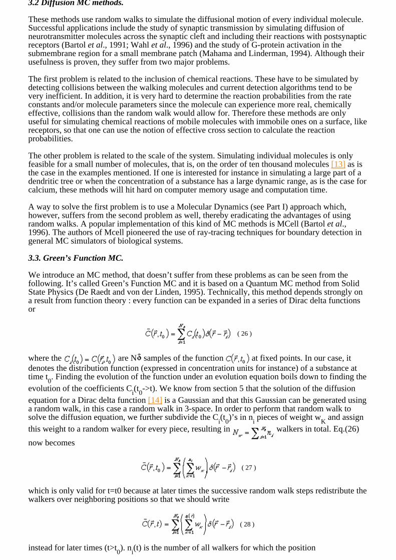
3.3. Green’s Function MC.

We introduce an MC method, that doesn’t suffer from these problems as can be seen from thefollowing. It’s called Green’s Function MC and it is based on a Quantum MC method from SolidState Physics (De Raedt and von der Linden, 1995). Technically, this method depends strongly ona result from function theory : every function can be expanded in a series of Dirac delta functionsor

( 26 )

where the are N samples of the function at fixed points. In our case, it denotes the distribution function (expressed in concentration units for instance) of a substance at time t

0. Finding the evolution of the function under an evolution equation boils down to finding the

evolution of the coefficients Ci(t

0->t). We know from section 5 that the solution of the diffusion

equation for a Dirac delta function [14] is a Gaussian and that this Gaussian can be generated using a random walk, in this case a random walk in 3-space. In order to perform that random walk tosolve the diffusion equation, we further subdivide the C

i(t

0)’s in n

i pieces of weight w

K and assign

this weight to a random walker for every piece, resulting in walkers in total. Eq.(26)

now becomes

( 27 )

which is only valid for t=t0 because at later times the successive random walk steps redistribute thewalkers over neighboring positions so that we should write

( 28 )

instead for later times (t>t0). n

i(t) is the number of all walkers for which the position

being a neighborhood of and , the

region in space in which the simulation takes place. When proper accounting of walkers is done,N

w=R

in

i(t) should be the initial number of walkers for every step.

The easiest way to perform the random walk, however, is to divide all Ci(t

0)’s in n

i equal pieces of

weight w. At time t, can now be approximated by

( 29 )

with ni(t) the number of walkers at or near. As a consequence, simulating diffusion has now

become as simple as taking Nw

samples of equal size w of the initial distribution function and keeping track of all the samples as they independently perform their random walks. In a closedregion V, choose weights w=(C

0V)/N

w where C

0 is for example the final concentration at

equilibrium and V=vol(V). For pure diffusion, all mass that was present initially will be preservedso that the weights stay unchanged. Note that N

w determines the variance of the fluctuations

around the expected mean [15] and can be much smaller than the number of molecules present in V. Therefore this Green’s Function MC method does not suffer from the same bad scaling properties as the diffusion MC methods.

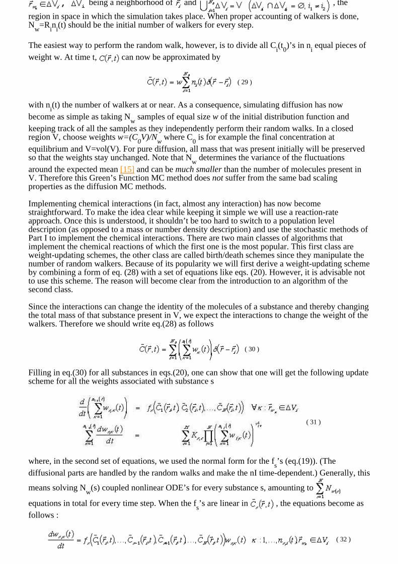
Implementing chemical interactions (in fact, almost any interaction) has now becomestraightforward. To make the idea clear while keeping it simple we will use a reaction-rateapproach. Once this is understood, it shouldn’t be too hard to switch to a population leveldescription (as opposed to a mass or number density description) and use the stochastic methods ofPart I to implement the chemical interactions. There are two main classes of algorithms thatimplement the chemical reactions of which the first one is the most popular. This first class areweight-updating schemes, the other class are called birth/death schemes since they manipulate thenumber of random walkers. Because of its popularity we will first derive a weight-updating schemeby combining a form of eq. (28) with a set of equations like eqs. (20). However, it is advisable notto use this scheme. The reason will become clear from the introduction to an algorithm of thesecond class.

Since the interactions can change the identity of the molecules of a substance and thereby changingthe total mass of that substance present in V, we expect the interactions to change the weight of thewalkers. Therefore we should write eq.(28) as follows

( 30 )

Filling in eq.(30) for all substances in eqs.(20), one can show that one will get the following updatescheme for all the weights associated with substance s

( 31 )

where, in the second set of equations, we used the normal form for the fs’s (eq.(19)). (The

diffusional parts are handled by the random walks and make the nI time-dependent.) Generally, this

means solving Nw

(s) coupled nonlinear ODE’s for every substance s, amounting to

equations in total for every time step. When the fs’s are linear in , the equations become as

follows :

( 32 )

with formal solution

( 33 )

where the approximation is assumed valid when the integrandum can be considered (nearly)constant in ]t,t+ t[. This update scheme guarantees positive weight values for positive initial values. Also, at a fixed position, the same exponential factor can be used for all the walkerscorresponding to the same substance, providing a significant optimisation. The accuracy andstability of the solution will depend on the problem at hand, especially the degree of stiffness willbe very important.

The term stiffness is generally used in the context of a coupled system of equations. It is a measurefor the range of time scales in the simultaneous solutions of the equations. If one is interested in thefast time scales, it implies that one will loose a lot of time calculating the slowly changingcomponents. If one is only interested in the slow components, it means that one runs the risk ofnumerical instability. Therefore special numerical algorithms should be applied to solve stiffsystems. Runge-Kutta-Fehlberg with Rosenbrock-type extensions are simple and robust examplesof such algorithms (see for example (Press et al., 1992)).

Sometimes the term ’stiffness’ is also used in the context of certain PDE’s. In this case it meansthat the spatial and temporal scale are linked by a relation like eq.(5). However, in most cases oneis interested in longer time scales for a fixed spatial scale than is prescribed by this relation. So,again, one is confronted with the dilemma of efficiency vs. numerical stability. Therefore also inthis case one should use numerical algorithms specially suited for these equations (for example theimplicit schemes as described in section 14).

Since the weights can change, nothing can stop them from becoming zero or very big. Walkerswith zero (or arbitrary subthreshold) weights don’t contribute (much) to the distribution function.Generating random walks for them is a waste of computation time. A popular practice is todisregard these small weight walkers all together (and possibly reuse their datastructures forredistributing large weight walkers, as described next). In case the weights become very large, theycan cause instability, excessive variance and huge numerical errors. Therefore one could divide awalker with a large weight into smaller pieces. There are other methods to increase efficiency andreduce variance but they depend on the specifics (like relative time scales) of the problem at hand.Without these weight control mechanisms, however, weight-update schemes tend to be veryinefficient and produce results with large variances.

Sherman and Mascagni (Sherman and Mascagni, 1994) developed a similar method, calledGradient Random Walk (GRW). Instead of calculating the solution directly, it calculates thegradient of the solution. Their work is a good source of references to other particle methods tosolve reaction-diffusion equations and to the mathematical foundations and computationalproperties of particle methods in general.

When using the combination of weight control mechanisms as described above, an importantprinciple of MC simulations is violated. This ’correspondence principle’ leads to the condition of’detailed balance’ [16] at thermodynamic equilibrium. It guarantees global balance (at thermodynamic equilibrium) and meaningful, consistent statistics (in general). A prerequisite for the correspondence principle to be met is to preserve the close correspondence-hence the name "correspondence principle"-between local changes in the distribution of random walkers and the physical processes that cause these local changes. This means that local reshuffling of random walkers for performance reasons is out of the question. Algorithms of the second class, however, meet this principle in an efficient manner when correctly implemented.

Deriving a particular scheme for second class algorithms starts from eq.(29) instead of eq. (28) :instead of making the weights dependent on time, like in eq.(30), one can find a scheme forchanging the number n

i(t) while keeping w

s fixed (on a per substance basis). By filling in eq.(29) in

eqs.(20) one gets for every position :

( 34 )

(now with which can be pre-computed). Now

one only has to solve N (<< Nw(s)

(t)) coupled nonlinear ODE’s for every position that isoccupied (by at least one substance), in the worst case scenario leading to at most

sets of N coupled equations of which most are trivial (i.e. zero change).

Integrating this set of equations over t gives a change in the number of random walkers n

i,s(t)(=n

i,s(t+ t)-n

i,s(t)) at position . Generally, n

i,s(t) is not an integer, therefore one uses the

following rule : [17] create/destroy ni,s

(t)V random walkers and create/destroy an extra

random walker with probability frac( ni,s

(t)). Note that now Nw

=Rin

i(t) is not preserved! The

correspondence principle is still met when globally scaling down the number of random walkers(and as a compensation renormalise their weight) for a substance in case their number has grownout of band due to nonFickian fluxes.

Now that one can select a method to incorporate chemical interactions, it has to be combined withthe discrete random walk generator for diffusion. To simplify the implementation, one chooses acommon spatial grid for all substances. Since for diffusion the temporal scale is intrinsically relatedto the spatial scale (by eq.(5)), this means a different t for every unique D. The simulation clockticks with the minimal t, t

min. Every clock tick, the system of eqs.(34) is solved to change the

numbers of random walkers. Then a diffusion step should be performed for every substance s forwhich an interval t

s has passed since its last diffusion update at time t

s. Here we made the

following implicit assumptions : the concentration of substance s in Vi is assumed not to change

due to diffusion during a time interval ts and all substances are assumed to be well-mixed in

every Vi. The assumptions are justified if one chooses vol( V

i) in such a way that in every V

ithe concentration changes every time step with atmost 10% for the fastest diffusing substance(s) (i.e. the one(s) with t

s= t

min).

3.4 Discretization in space and time.

For a large enough number of molecules, it is sufficient to integrate the diffusion equations directlyusing for instance discretisation methods. Their scaling properties are much better (although, formulti-dimensional problems this is questionable) and, theoretically, they are also much faster.However, as can be seen from the equations (see below), their implementation can become moreand more cumbersome for every additional interaction term and for growing geometricalcomplexity. So, although these methods are very popular because of their perceived superiorperformance, it’s sometimes more feasible to use the Green’s Function MC method (or anotherequivalent particle method) as a compromise between performance and ease of implementation.

The Crank-Nicholson method is an example of a classical implicit finite difference discretisationmethod that is very suited for diffusion problems. Section 15 introduces the formulation forone-dimensional (reaction-)diffusion and section 16 provides ADI, an extension toCrank-Nicholson to solve multi-dimensional problems.

3.5 One-dimensional diffusion.

Because the diffusion equation (eq.(6)) is a parabolic PDE-which makes it very stiff for mostspatial scales of interest (Carnevale, 1989; Press et al., 1992)-its solution prefers an implicit [18]solution method and its numerical solution is sensitive to the accuracy of the boundary conditions (Fletcher, 1991). For the discretisation, the volume will be split in a number of elements and the concentration is computed in each of them. This approximation for a real concentration will be good if sufficient molecules are present in each element so that the law of large numbers applies. This implies that the elements should not be too small, though this may of course lead to a loss of accuracy in representing gradients. The problem is not trivial. Take, for example, the calcium concentration in a dendritic spine (Koch and Zador, 1993). A resting concentration of 50 nM corresponds to exactly two calcium ions in the volume of a 0.5 m diameter sphere, which is about

the size of a spine head! The random walk methods described in the previous sections seem moreappropriate for this situation.

A popular assumption is that of a spherical cell where diffusion is modeled using the sphericalradial equation (2nd eq. of eqs.(16)). The discretisation is performed by subdividing the cell into aseries of onion shells with a uniform thickness of about 0.1 m (Blumenfeld et al., 1992) andfigs.3-5). The Crank-Nicolson method is then the preferred solution method for finding theconcentration in each shell after every time step t (Fletcher, 1991; Press et al., 1992) as it isunconditionally stable and second order accurate in both space and time. We will continue usingour example of calcium diffusion, which leads to a set of difference equations of the form:

( 35 )

Note that the equations express the unknown in terms of the knowns (the right-hand

side terms) but also of the unknowns for the neighboring shells. Therefore, this requires an iterativesolution of the equations, which is typical for an implicit method. The terms containing i+1 areabsent in the outer shell i=n and those containing i-1 in the innermost shell i=0. This system ofequations can be applied to any one-dimensional morphology, where the geometry of the problemis described by the coupling constants C

i,i+1. In the case of a spherical cell the coupling constants

are of the form :

( 36 )

where r is the uniform thickness of the shells and the diameter of the cell is equal to d=2n r. See De Schutter and Smolen (1998) for practical advise on how to apply these equations to morecomplex geometries.

The system of algebraic equations eqs.(35) can be solved very efficiently because its correspondingmatrix is tridiagonal with diagonal dominance (Press et al., 1992). Influx across the plasma membrane can be simulated by adding a term to the right-hand side of the

equation corresponding to the outer shell. Computing the flux at t+ t/2 maintains the second orderaccuracy in time (Mascagni and Sherman, 1998). Note that the overall accuracy of the solution willdepend on how exactly this boundary condition Jn is met (Fletcher, 1991).

In the case of buffered diffusion the buffer reaction eq.(22) has to be combined with eqs.(35). Thisleads to a new set of equations with for every shell one equation for each diffusible buffer:

( 37 )

and an equation for buffered calcium diffusion:

( 38 )

Equation (38) applies to a system with only one buffer. In case of multiple buffers, one additionalterm appears at the left-hand side and two at the right-hand side for each buffer. We have alsoassumed that DB is identical for the free and bound forms of the buffer, which gives a constant[B]

T,I. This is reasonable taking into account the relative sizes of calcium ions as compared to most

buffer molecules.

Eqs.(37) and (38) should be solved simultaneously, resulting in a diagonally banded matrix withthree bands for the calcium diffusion and two bands extra for each buffer included in the model.

3.6 Two-dimensional diffusion.

An elegant extension to the Crank-Nicholson method is the Alternating Direction Implicit (ADI)method which allows for an efficient solution of two-dimensional diffusion problems (Fletcher,1991; Press et al., 1992). Each time step is divided into two steps of size t/2 and in each substepthe solution is computed in one dimension:

( 39 )

respectively

( 40 )

where first diffusion along the i dimension is solved implicitly and then over the j dimension. Thecoupling constants C

i,i+1 and c

j,j+1 again depend on the geometry of the problem and are identical

and constant in the case of a square grid. The two matrices of coupled equations (39) and (40) aretridiagonal with diagonal dominance and can be solved very efficiently. In two dimensions, theADI method is unconditionally stable for the complete time step and second order accurate in bothspace and time, provided the appropriate boundary conditions are used (Fletcher, 1991). Holmes(Holmes, 1995) used the two-dimensional ADI method with cylindrical coordinates to modelglutamate diffusion in the synaptic cleft. The ADI method can also be applied to simulatethree-dimensional diffusion with substeps of t/3, but in this case it is only conditionally stable(Fletcher, 1991).

4 Case study.

In general, we’re interested in compartmental models of neurons using detailed reconstructedmorphologies, in particular of the dendritic tree. These compartments are cylindrical idealisations

of consecutive tubular sections of dendritic membrane. Because of the cylindrical nature of thecompartments we prefer a description in cylindrical coordinates, giving us an accuraterepresentation of the concentration in the submembrane region. This is important for a number ofour other simulations. As can be seen from eq.(15), using cylindrical coordinates introduces factorsdepending on 1/ and an additional first-order term in . These are pure geometric effects and arisefrom the fact that an infinitesimal volume element in cylindrical coordinates is of the form dV= d

d dz which is dependent on .

Just like in the 1D case, eq.(11)(2nd eq.) can be derived from a (discrete) random walk process.That is, in Cartesian coordinates, for every second order term on the right-hand side of eq. (11)(2nd

eq.) the corresponding coordinate of the random walker’s position is updated according to the 1Drandom walk scheme. However, this recipe does not work when writing out a random walk schemefor eq.(14) due to the extra first-order term. A more general recipe for deriving the appropriaterandom walk process can be obtained by considering more closely the consequences of the -dependency of dV.

In order to maintain a uniform distribution of mass at equilibrium, there should be less mass in thevolume elements closer to the origin, since for smaller , i.e. nearer to the origin, the volume elements get smaller. Therefore the random walkers (which correspond to mass units) should tend to step more often away from the origin than toward the origin when equilibrating, creating a net drift outward. Eventually, in a closed volume with reflecting walls this drift will come to a halt at equilibrium, while the outward tendency creates a gradient in in the number (but not density!) ofwalkers. The tendency is introduced by adjusting the probability to choose the direction of a -step.

The adjustment is derived as follows for a drifting 1D random walk : suppose the walkers have adrift speed c (negative to go to the left, positive to go to the right) then the probability to go to theleft is

( 41 )

(with obvious conditions on t and x for a given c). When filling in these expressions for pl,r ineq.(1) and taking the appropriate limits, one gets the following equation

( 42 )

Note the correspondence between this equation and the radial part of eq.(14). Therefore we extendthe recipe as follows : every first-order term corresponds to a drift with the drift speed c given bythe coefficient of the partial derivative and the probabilities are adjusted according to eq.(41). If weignore the 1/ factors by defining new ’constants’ c=D/r and D’=D/r2, we get the following random walk scheme in cylindrical coordinates : for every time step t->t+ t, for every walker

the following coordinate update is performed :

( 43 )

where we choose

( 44 )

with the following probabilities for the respective signs :

( 45 )

and (pr-=0, pr

+=1) for k=0. This type of random walk is called a Bessel walk. From the 1/rn factors

in the diffusion equation one expects problems of divergence in the origin. The way we handle therandom walks in the origin (i.e. for k=0) seems to work fine as can be seen from simulation results.Of course, due to the low number of walkers in the origin, the variance is quite large in the regionaround the origin.

The discrete natures of the geometry and the random walk introduce other specific problems,among which are connections of compartments with different radii, branchpoints and regions ofspine neck attachments to the compartmental mantle. We used minimalistic approaches to theseproblems by using probabilistic models. Concerning the connections for example, we assigned aprobability for the transition that the random walker could make between two connected cylindersin such a way that pz+/- becomes

( 46 )

(where the sign is chosen in accordance with the end of the cylinder at which the walker is) in casethe walker is at the end of cylinder 1 that is connected to cylinder 2. When the walker makes thetransition to cylinder 2, its -coordinate is adjusted according to

new=(R

2/R

1)

old. This way no

artificial gradients are created in the area around the discrete transition. Instead, the walkers behavemore like walkers in a tapered cylinder, which is the more natural geometry for dendritic branches.

Fig. 6: The effect of the presence of spines on the longitudinal component of diffusion in the dendritic shaft. Compare with fig.1 for the smooth case (i.e. without spines). The yellow dots represent (small sphere-like) molecules. In the model, the spine heads-the small spheres on the spine necks shown here as sticks perpendicular to the dendritic shaft-are modeled as short, wide cylinders.

Recent caged compound release experiments in neuronal spiny dendrites (Wang and Augustine,1995) and (Bormann et al., 1997) show a slowing in the apparent diffusion (see fig.6). The apparent diffusion constant is defined as the diffusion constant for the effective 1D diffusion along the longitudinal axis of the dendritic shaft. The experiments were performed with both relativelyinert and highly regulated substances. We were interested in estimating the contribution ofgeometric factors to this slowing in apparent diffusion rate, especially the effect of ’hidden’volume (mostly spines) and morphology (branching, structures in cytoplasm).

In order to isolate the contributing factors, we constructed simple geometrical models of dendriticstructures including spines and single branchpoints. Then we simulated idealised releaseexperiments by using square pulses as initial condition and calculated the apparent diffusioncoefficient D

app(t) from the resulting concentration profiles as follows :

( 47 )

with

( 48 )

The integral is cut off at the endpoints of the (chain of consecutive) cylinders, which is ok when thedistance between the endpoints is large enough so that only very few walkers will arrive at either ofthe endpoints in the simulated time period. The simulator is instructed to output

, i.e. the - and -dependence is averaged out. Slowing is expressed by aslowing factor (t), defined as . The apparent diffusion constantD

app at equilibrium is defined as D

app=D

app(t-> ).

Fig.7 shows the difference in time evolution of two concentration profiles. One is for a smoothdendrite (modeled as a simple cylinder), the other for a spiny dendrite of the same length but withspines distributed over its plasma membrane. The spines are attached perpendicularly on thecylindrical surface and consist of 2 cylinders : one narrow for the neck (attached to the surface) andone wide for the head. The figure shows the results for the most common spines parameters(density, neck and head lengths and radii) on Purkinje cell dendrites.

Fig. 7: Concentration profiles along length axis of the dendritic shaft.

Upper frame : Smooth dendrite case (see text).

Lower frame : Spiny dendrite case (see text).

The corresponding (t) curves can be found, overlapped, in fig.8. The small amount of slowing in the smooth dendrite case is due to reflection at the endpoints, which is neglectible for the period ofsimulation time used. We found (0)/ ’s of 1.0-3.0 for various geometric parameters of thespines. (We used (0)/ to express total slowing instead of -1 because D

app(0) is only

equal to D for initial conditions that are solution of the diffusion equation.)

Fig. 8: Slowing factor curves.

Red curve Spiny dendrite case (see text).

Blue curve Smooth dendrite case (see text).

5 Conclusion.

In this chapter we have demonstrated that diffusional processes can dominate the kinetics ofmolecular processes. Moreover, in many cases the effect of diffusion is strongly influenced by theboundary conditions, in particular by the local geometry of the cell in all three dinensions.However, most models of reaction-diffusion systems to date have assumed some form of spatialsymmetry so that they could be reduced to a one-dimensional system. As a consequence, efficientmethods to simulate three-dimensional reaction-diffusion systems are still under development.

REFERENCES

Albritton ML, Meyer T, Stryer L (1992) Range of messenger action of calcium ion and inositol1,4,5-triphosphate. Science 258:1812-1815.

Augustine GJ, Charlton MP, Smith SJ (1985) Calcium entry and transmitter release atvoltage-clamped nerve terminals of squid. J Physiol 367:163-181.

Baimbridge KG, Celio MR, Rogers JH (1992) Calcium-binding proteins in the nervous system.Trends Neurosci 15:303-308.

Bartol TM, Land BR, Salpeter EE, Salpeter MM (1991) Monte Carlo simulation of miniatureend-plate current generation in the vertebrate neuromuscular junction. Biophys J 59:1290-1307.

Bartol TMJ, Stiles JR, Salpeter MM, Salpeter EE, Sejnowski TJ (1996) MCELL: GeneralisedMonte Carlo computer simulation of synaptic transmission and chemical signaling. Abstr SocNeurosci 22:1742.

Berridge MJ (1997) The AM and FM of calcium signaling. Nature 386:759-760.

Bezprozvanny I (1994) Theoretical analysis of calcium wave propagation based on inositol(1,4,5)-triphosphate (InsP3) receptor functional properties. Cell Calcium 16:151-166.

Bezprozvanny I, Watras J, Ehrlich BE (1991) Bell-shaped calcium-dependent curves ofIns(1,4,5)P3-gated and calcium-gated channels from endoplasmic reticulum of cerebellum. Nature351:751-754.

Blumenfeld H, Zablow L, Sabatini B (1992) Evaluation of cellular mechanisms for modulation ofcalcium transients using a mathematical model of fura-2 Ca2+ imaging in Aplysia sensory neurons.Biophys J 63:1146-1164.

Bormann G, Wang SS-H, De Schutter E, Augustine GJ (1997) Impeded diffusion in spinydendrites of cerebellar Purkinje cells. Abstr Soc Neurosci 23:2008.

Bower JM, Beeman D. (1995). The book of GENESIS: exploring realistic neural models with theGEneral NEural SImulation System. New York, NY: TELOS.

Carnevale NT (1989) Modeling intracellular ion diffusion. Abstr Soc Neurosci 15:1143.

Crank J. (1975). The mathematics of diffusion. Oxford, U.K.: Clarendon Press.

De Raedt H, von der Linden W. (1995). The MC method in condensed matter physics. (2nd Ed.ed.). (Vol. 71). Berlin: Springer-Verlag.

De Schutter E, Smolen P. (1998). Calcium dynamics in large neuronal models. In: Methods inneuronal modeling: from ions to networks (Koch C & Segev I, ed.^eds.) (2nd ed., ), pp. 211-250.Cambridge, MA: MIT Press.

DiFrancesco D, Noble D (1985) A model of cardiac electrical activity incorporating ionic pumpsand concentration changes. Phil Trans Roy Soc London Ser B 307:353-398.

Dolmetsch RE, Xu K, Lewis RS (1998) Calcium oscillations increase the efficiency and specificityof gene expression. Nature 392:933-936.

Einstein A (1905) On the movement of small particles suspended in a stationary liquid demandedby the molecular kinetics of heat. Ann Phys 17:549-560.

Exton JH (1997) Phospholipase D: enzymology, mechanisms of regulation, and function. PhysiolRev 77:303-320.

Farnsworth CL, Freshney NW, Rosen LB, Ghosh A, Greenberg ME, Feig LA (1995) Calciumactivation of Ras mediated by neuronal exchange factor Ras-GRF. Nature 376:524-527.

Feynman RP, Leighton RB, Sands M. (1989). The Feynman Lectures on Physics (CommemorativeIssue): Addison-Wesley.

Fick A (1885) Ueber Diffusion. Ann Phys Chem 94:59-86.

Fishman GS. (1996). Monte Carlo : Concepts, Algorithms and applications.: Springer-Verlag.

Fletcher CAJ. (1991). Computational techniques for fluid dynamics. Volume I. Berlin:Springer-Verlag.

Foley J, Van Dam A, Feiner S, Hughes J. (1990). Computer graphics : principles and practice. (2nded.): Addison-Wesley.

Garrahan PJ, Rega AF. (1990). Plasma membrane calcium pump. In: Intracellular calciumregulation (Bronner F, ed. eds.) , pp. 271-303. New York: Alan R. Liss.

Gola M, Crest M (1993) Colocalization of active KCa channels and Ca2+ channels within Ca2+

domains in Helix neurons. Neuron 10:689-699.

Goldbeter A, Dupont G, Berridge MJ (1990) Minimal model for signal-induced Ca2+ oscillations and for their frequency encoding through protein phosphorylation. Proc Natl Acad Sci USA87:1461-1465.

Hille B. (1992). Ionic channels of excitable membranes. Sunderland: Sinauer Associates.

Holmes WR (1995) Modeling the effect of glutamate diffusion and uptake on NMDA andnon-NMDA receptor saturation. Biophys J 69:1734-1747.

Issa NP, Hudspeth AJ (1994) Clustering of Ca2+ channels and Ca2+-activated K+ channels at fluorescently labeled presynaptic active zones of hair cells. Proc Natl Acad Sci USA91:7578-7582.

Jafri SM, Keizer J (1995) On the roles of Ca2+ diffusion, Ca2+ buffers, and the endoplasmic reticulum in IP3-induced Ca2+ waves. Biophys J 69:2139-2153.

Kasai H, Petersen OH (1994) Spatial dynamics of second messengers: IP3 and cAMP aslonge-range and associative messengers. Trends Neurosci 17:95-101.

Koch C, Zador A (1993) The function of dendritic spines: devices subverving biochemical ratherthan electrical compartmentalization. J Neurosci 13:413-422.

Li W, Llopis J, Whitney M, Zlokarnik G, Tsien RY (1998) Cell-permeant caged InsP3 ester showsthat Ca2+ spike frequency can optimize gene expression. Nature 392:936-941.

Linse S, Helmersson A, Forsen S (1991) Calcium-binding to calmodulin and its globular domains.J Biol Chem 266:8050-8054.

Llano I, DiPolo R, Marty A (1994) Calcium-induced calcium release in cerebellar Purkinje cells.Neuron 12:663-673.

Llinás RR, Sugimori M, Silver RB (1992) Microdomains of high calcium concentration in apresynaptic terminal. Science 256:677-679.

Mahama PA, Linderman JJ (1994) A Monte Carlo study of the dynamics of G-protein activation.Biophys J 67:1345-1357.

Markram H, Roth A, Helmchen F (1998) Competitive calcium binding: implications for dendritic

calcium signaling. J Comput Neurosci 5:331-348.

Mascagni MV, Sherman AS. (1998). Numerical methods for neuronal modeling. In: Methods inneuronal modeling: from ions to networks (Koch C & Segev I, ed. eds.) (2nd ed., ), pp. 569-606.Cambridge, MA: MIT Press.

Naraghi M, Neher E (1997) Linearized buffered Ca2+ diffusion in microdomains and itsimplications for calculation of [Ca2+] at the mouth of a calcium channel. J Neurosci 17:6961-6973.

Nixon RA (1998) The slow axonal transport of cytoskeletal proteins. Curr Opin Cell Biol10:87-92.

Nowycky MC, Pinter MJ (1993) Time courses of calcium and calcium-bound buffers followingcalcium influx in a model cell. Biophys J 64:77-91.

Press WH, Teukolsky SA, Vetterling WT, Flannery BP. (1992). Numerical recipes in C: The art ofscientific computing. (2nd ed.). Cambridge: Cambridge University Press.

Qian N, Sejnowski TJ (1990) When is an inhibitory synapse effective? Proc Natl Acad Sci USA87:8145-8149.

Regehr WG, Atluri PP (1995) Calcium transients in cerebellar granule cell presynaptic terminals.Biophys J 68:2156-2170.

Sala F, Hernandez-Cruz A (1990) Calcium diffusion modeling in a spherical neuron: relevance ofbuffering properties. Biophys J 57:313-324.

Schulman LS. (1981). Techniques and applications of path integration. New York, N.Y.: JohnWiley & Sons.

Sherman A, Mascagni M (1994) A gradient random walk method for two-dimensionalreaction-diffusion equations. SIAM J Sci Comput 15:1280-1293.

Sneyd J, Charles AC, Sanderson MJ (1994) A model for the propagation of intracellular calciumwaves. Amer J Physiol 266:C293-C302.

Sneyd J, Wetton BTR, Charles AC, Sanderson MJ (1995) Intercellular calcium waves mediated bydiffusion of inositol triphosphate: a two-dimensional model. Amer J Physiol 268:C1537-C1545.

Wagner J, Keizer J (1994) Effects of rapid buffers on Ca2+ diffusion and Ca2+ oscillations. Biophys J 67:447-456.

Wahl LM, Pouzat C, Stratford KJ (1996) Monte Carlo simulation of fast excitatory synaptictransmission at a hippocampal synapse. J Neurophysiol 75:597-608.

Wang SS-H, Augustine GJ (1995) Confocal imaging and local photolysis of caged compounds:dual probes of synaptic function. Neuron 15:755-760.

Zador A, Koch C (1994) Linearized models of calcium dynamics: formal equivalence to the cableequation. J Neurosci 14:4705-4715.

Zhou Z, Neher E (1993) Mobile and immobile calcium buffers in bovine adrenal chromafin cells. JPhysiol 469:245-273.

Page last updated on Friday, 07-Jun-2002 12:09:08 CEST © BBF 1998 all rights

reserved

about us publications models servers courses search

contact software lab only home

[NO FRAMES]

[RELOAD FRAMES AND HOMEPAGE]

Please send comments and suggestions to Mike Wijnants.